Theor. Comput. Fluid Dyn. (2011) 25:179–193DOI 10.1007/s00162-010-0194-6

ORIGINAL ARTICLE

Philippe Meliga · Jean-Marc Chomaz

Global modes in a confined impinging jet: applicationto heat transfer and control

Received: 22 May 2009 / Accepted: 3 December 2009 / Published online: 30 March 2010© Springer-Verlag 2010

Abstract We investigate the stability and control of a plane, laminar jet impinging on a flat plate in a channel,a geometry used to cool down a hot wall with a cold air jet in many industrial configurations. The global stabil-ity analysis indicates that, even for a strong confinement, the two-dimensional (2-D) steady flow is unstable tothree-dimensional (3-D), steady perturbations. In the simplest limit case where dilatation effects are neglected,we show that the development of the instability induces a significant spanwise modulation of the heat fluxat the impacted wall. To control the leading global mode, we propose adjoint-based 3-D harmonic and 2-Dsteady forcing in the bulk or at the wall. We show for instance that the unstable mode is controllable using aspanwise uniform blowing at the upper wall, in a specific domain corresponding to the footprint of the upperrecirculating bubble. These techniques are applied to a novel open-loop control, in which we introduce intothe flow a small airfoil, modelled by the lift force it exerts on the flow.

Keywords Impinging jet · Global instability · Wavemaker · Control · Lift

1 Introduction

Jet impingement is widely used in many industrial and engineering applications when an intense and rapid heattransfer is desired, for instance the tempering of metal sheets, the cooling of electronic components and turbineblades, or the drying of papers and textiles. The main advantage of this technique lies in the high localizationof the cooling, as the use of high-speed jets allows to remove a large amount of heat on the impinging surface,around the stagnation region. It has been generally acknowledged that the use of such jets enhances the localtransfer by more than an order of magnitude, compared to classical wall boundary layers [18].

A large body of works has been devoted to the study of impinging jet flows, including the effect of thejet geometry (circular, rectangular or plane cross-section), the nature of the impacted surface (plane, inclinedor with obstacles) and the Reynolds number at the jet exit ([21] for a review). In many applications, the jet isoperated in the laminar or transitional regime, due to the smallness of the scales involved. The jet is also often

Communicated by T. Colonius

P. Meliga (B), J.-M. ChomazLadHyX-CNRS, Ecole Polytechnique, 91128 Palaiseau, FranceE-mail: philippe.meliga@ladhyx.polytechnique.fr

J.-M. ChomazE-mail: jean-marc.chomaz@ladhyx.polytechnique.fr

Present address:P. MeligaLFMI, Ecole Polytechnique Fédérale de Lausanne, 1015 Lausanne, SwitzerlandE-mail: philippe.meliga@epfl.ch

180 P. Meliga, J.-M. Chomaz

confined between the target surface and an opposing surface in which the jet orifice is located, so as to increasethe efficiency of the heat transfer. The presence of a confining top surface then results in a complex flow inwhich the behavior of the free jet is coupled to that of the channel flow developing between the two surfaces.

Only a limited amount of studies is available about highly confined, low Reynolds number jets. Thesteady and unsteady dynamics of a laminar two-dimensional (2-D) jet impinging on a flat plate have beeninvestigated numerically [4,13] and experimentally [22] for various Reynolds numbers and levels of confine-ment 2 ≤ H/e ≤ 9, where H is the distance from the jet exit to the wall and e is the jet width. In particular,the direct numerical simulations (DNS) carried out by Lee et al. [13] on the most confined configuration(H/e = 2) show that the flow bifurcates from a 2-D steady to a 2-D unsteady state at Re ∼ 1050, where Reis the Reynolds number built from the channel height and the centerline velocity. However, these studies failto consider the three-dimensional (3-D) aspects of the flow, which are crucial when spanwise homogeneoustransfers are desired. For instance, for automotive purposes, steel sheets are coated by a zinc layer in orderto resist to oxidization. Moving steel strips are dipped into a bath of molten zinc and then cooled down byimpinging jets before being rolled up and sent to car manufacturers. Inhomogeneous protective zinc layers aretherefore detrimental to the whole manufacturing process and should be alleviated.

In this study, we carry out the global stability analysis of a strongly confined jet of height ratio H/e = 2,and show that the 2-D steady solution is unstable to 3-D steady disturbances. We characterize the effect of theinstability on the heat flux at the impacted wall, as a way to illustrate the practical effect of global modes inindustrial configurations. We also investigate adjoint-based control strategies for this global instability, usingtechniques introduced by Hill [12]. We discuss forcing methods that can be either 2-D steady or 3-D harmonic.The results are applied to a novel control strategy where a small airfoil is introduced into the flow. This controlacts through the lift component of the force it exerts on the flow and differs from the classical control by meansof a small cylinder, which acts through the drag component of the force.

2 Problem formulation

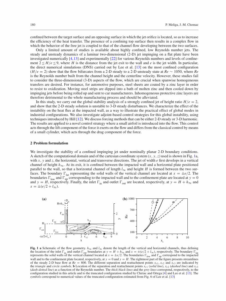
We investigate the stability of a confined impinging jet under nominally planar 2-D boundary conditions.A sketch of the computational domain and of the cartesian coordinate system (x, y, z) used is shown in Fig. 1a,with x, y and z, the horizontal, vertical and transverse directions. The jet of width e first develops in a verticalchannel of height h∞. At its exit, it is confined between the impacted wall and a horizontal plate positionedparallel to the wall, so that a horizontal channel of length l∞ and height H is formed between the two sur-faces. The boundary �lat representing the solid walls of the vertical channel are located at x = ±e/2. Theboundaries �low and �up corresponding to the impacted wall and to the confinement plate are located at y = 0and y = H , respectively. Finally, the inlet �in and outlet �out are located, respectively, at y = H + h∞ andx = ±(e/2 + l∞).

x

y

-3 0 3 6 90

2

Γlow

Γout

Γin

Γlat

ΓupH -e/2

∞H+h

∞

(a)

x r2 xr3

xr1

-(e/2+l )

xr

Re

0 2 4 6 8 10

100

400

700

1000(b)

Fig. 1 a Schematic of the flow geometry. h∞ and l∞ denote the length of the vertical and horizontal channels, thus definingthe location of the inlet �in and outlet �out boundaries at y = H + h∞ and x = ±(e/2 + l∞), respectively. The boundary �latrepresents the solid walls of the vertical channel located at x = ±e/2. The boundaries �low and �up correspond to the impactedwall and to the confinement plate located, respectively, at y = 0 and y = H . The rightmost part of the figure presents streamlinesof the steady 2-D base flow at Re = 800. The different separation and reattachment points xr1, xr2 and xr3 are indicated bythe triangle and circle symbols. b Location of the separation and reattachment points xr1 (solid line), xr2 (dashed line) and xr3(dash-dotted line) as a function of the Reynolds number. The thick black lines and the grey lines correspond, respectively, to theconfiguration studied in this article and to the truncated configuration studied by Chiriac and Ortega [4] and Lee et al. [13]. Thesymbols correspond to numerical values of the truncated configuration estimated from Fig. 6 of Lee et al. [13]

Global modes in a confined impinging jet 181

In the following, we set the height ratio to H/e = 2. All quantities are made non-dimensional usingthe height H and the jet centerline velocity. The state vector q stands for the flow field (u, p)T, whereu = (u, v, w)T is the fluid velocity with u, v and w, the x, y and z-velocity components; p is the pressure andT designates the transpose. The fluid motion is governed by the incompressible Navier–Stokes equations

∇ · u = 0, ∂tu + ∇u · u + ∇ p − Re−1∇2u = 0. (1)

We use a parabolic velocity profile u = (2x − 1) (2x + 1) ey at the inlet, no-slip conditions on the solid wallsand a free outflow condition −pn + Re−1∇u · n at the outlet. Since the whole configuration is symmetricwith respect to the jet axis of symmetry, all flow field quantities can be split into symmetric and antisymmetricfields. However, such symmetries are not explicitly imposed in this study, namely the whole configuration ismeshed and no boundary conditions are imposed at the jet axis.

The state vector q is decomposed into a steady 2-D base flow Q and a 3-D perturbation q ′ of infinitesimalamplitude ε. The base flow is searched as a steady solution Q = (U, V, 0, P)T satisfying the 2-D equations

∇ · U = 0, ∇U · U + ∇P − Re−1∇2U = 0. (2)

All perturbations are chosen in the form of normal eigenmodes of spanwise wavenumber k and complex pul-sation σ + iω, σ and ω being, respectively, the growth rate and the pulsation of the eigenmode (σ > 0 for anunstable eigenmode):

q ′ = q(x, y)e(σ+iω)t+ikz + c.c. (3)

In (Eq. 3), q = (u, v, w, p)T is the so-called global mode, for which both the horizontal and the verticaldirections (x, y) are eigendirections, and c.c. denotes the complex conjugate of the preceding expression. Thisyields the generalized eigenvalue problem for λ = σ + iω and q:

∇ · u = 0, λu + ∇u · U + ∇U · u + ∇ p − Re−1∇2u = 0, (4)

the boundary conditions consisting of a Dirichlet condition u = 0 at the inlet and the solid walls, and of a freeoutflow condition − pn + Re−1∇u · n = 0 at the outlet.

The FreeFem++ software1 is used to generate a mesh composed of triangular elements with the Delaunay–Voronoi algorithm. The mesh refinement is controlled by the vertex densities on both external and internalboundaries. The base flow and disturbance equations are numerically solved by a finite-element method, usingthe same mesh. The unknown velocity and pressure fields are spatially discretized using a basis of Taylor–Hoodelements, i.e. P2 elements (6 degrees of freedom) for velocities and P1 elements (3 degrees of freedom) forpressure. The associated variational formulations are derived and spatially discretized on the mesh, and thesparse matrices resulting from the projection of the variational formulations onto the basis of finite elementsare built with the FreeFem++ software.

The base flow Q, solution of the steady, 2-D, non-linear equations (2) is obtained using an iterative Newtonmethod [1]. Starting from any guess value Q, presently obtained by time-marching a DNS of equations (1)along with the required boundary conditions, this method involves the resolution of simple linear problems.At each step, a matrix inversion is performed using the UMFPACK library, which consists in a sparse directLU solver [7]. The spatial discretization of problem (4) results in a large-scale generalized eigenvalue prob-lem, solved using the “Implicitly Restarted Arnoldi method” of the ARPACK library2 based upon a shift andinvert strategy [8]. All global modes are normalized by imposing the phase of the x-velocity component tobe zero at x = 10 and y = 0.5, i.e. u(10, 0.5) is real positive. The eigenmode energy is then normalized tounity in a fixed domain �in defined arbitrarily as |x | ≤ 8.125 and y ≤ 3, so that

∫�in

|u|2(x, y)d� = 1. Thisnormalization choice has no effect on the results presented here. It is simply used to test the convergence ofcomplex eigenvectors when computed on various domain sizes.

1 http://www.freefem.org.2 http://www.caam.rice.edu/software/ARPACK.

182 P. Meliga, J.-M. Chomaz

3 Results

3.1 Base flow computations

The rightmost part of Fig. 1a shows the streamlines of the symmetric base flow computed at Re = 800. Itexhibits a first separation bubble extending at the upper wall from the edge of the nozzle to the horizontalposition xr1, and a second separation bubble at the lower wall extending from xr2 to xr3. The location ofthese points, illustrated by the symbols sketched in Fig. 1a, is presented for various Reynolds numbers as thethick black solid, dashed and dash-dotted lines in Fig. 1b. We find that the second separation zone appears forRer2 � 330. Close to this threshold value, the size of this second region, defined as Lr2 = xr3 − xr2, scales asLr2 ∝ (Re − Rer2)

1/2 (not shown here). The grey lines in Fig. 1b correspond to base flow calculations carriedout on the truncated configuration studied by Chiriac and Ortega [4] and Lee et al. [13], values estimated fromthis last study being also reported as the grey triangle and circle symbols. In their studies, these authors haveset the height of the vertical channel to h∞ = 0 and have imposed a uniform velocity profile directly at the jetexit, i.e. flush with the upper wall, meaning that the dynamics of the free jet is no more coupled to that of thefluid in the horizontal channel. Our results precisely show that the location of the separation and reattachmentpoints is very sensitive to the jet velocity profiles, as their position is systematically underestimated in thetruncated configuration. This outlines the importance of including the vertical channel in the computation ofimpinging jet flows.

3.2 Two-dimensional global modes

We find that the base flow is stable to any 2-D disturbances in the range of Reynolds numbers under con-sideration: Fig. 2a shows the evolution of the growth rate of the two leading 2-D modes as a function of theReynolds number, up to Re = 1400. These modes are stationary (ω = 0), and exhibit small negative growthrates (σ < 0 and |σ | � 1), meaning that they are very slowly damped. The leading global mode is antisym-metric, whereas the second leading mode is symmetric. We recall here that the symmetry of the modes has notbeen enforced in the numerics, but emerges spontaneously from the computations even with a non-symmetriccomputational grid. In the following, the eigenvectors corresponding to these antisymmetric and symmetricmodes are referred to q0,a and q0,s , respectively. The effect of these modes can be physically interpreted byconsidering the flow reconstructed as the linear superposition of the base flow Q and the global modes q0,aand q0,s with a finite amplitude ε. For both the modes, ε has been set so that the energy of the global moderepresents 0.25% that of the base flow. Figure 3 shows the separation lines of the base flow and of the totalflow Q + εq as the dashed and solid lines, respectively, whereas the levels of energy of the total flow areindicated by the colour shading. The main effect of the 2-D modes is to shift the location of the separation andreattachment points (up to 9% for the chosen perturbation amplitude). The slow dynamics associated to theseweakly damped modes has therefore an important impact if one aims at obtaining precise approximations ofthe steady state using a time-marching procedure [4,13], since the simulation must last long enough for these

Re

σ

400 600 800 1000 1200 1400-0.06

-0.04

-0.02

0(a)

k

σ

9 6 3 0 3 6 9-0.05

-0.025

0

0.025(b)

Fig. 2 a Growth rate of the two leading 2-D global modes as a function of the Reynolds number. The black symbols correspondto the Reynolds number Re = 900 for which the complete eigenvalue spectrum is shown in (b). b Eigenvalue spectrum inthe (k, σ )-plane for Re = 900. The light grey shaded area stands for the stable domain σ ≤ 0. The right and left half-planescorrespond to antisymmetric and symmetric modes, respectively, whereas the white and dark grey symbols denote steady andoscillating modes. The black symbols correspond to the leading 2-D modes reported in (a) for this Reynolds number

Global modes in a confined impinging jet 183

y

�9 �6 �3 0 3 6 90

2(a)

x

y

�9 �6 �3 0 3 6 90

2(b)

0 1

0 1

Fig. 3 Physical effect of the 2-D modes at Re = 800. The dashed and solid lines stand for the separation lines of the base flow andof the total flow Q+εq, respectively. ε has been set so that the perturbation energy represents 0.25% of the base flow energy. Thecolour shading depicts the spatial distribution of energy of the total flow, and the white hue corresponds to vanishing amplitudes.a Antisymmetric mode q0,a , b symmetric mode q0,s

modes to reach a small enough amplitude. For the amplitude to decay by n orders of magnitude, the simulationshould last at least 2.3n/|σ0,max|, where σ0,max is the largest growth rates over all 2-D modes. Practically, fora Reynolds number Re = 800 and n = 3, i.e. a decrease of 10−3 in the amplitude of the departure from theexact steady state, this requires to run the numerical simulation for more than 500 times the advection timescale. This justifies the present use of the Newton iterative algorithm, which allows to compute steady statesin about five iterations only, the residual of the governing equations being then smaller than 10−12.

3.3 3-D global modes

Figure 2b presents the eigenvalue spectrum for both 2-D and 3-D modes at the Reynolds number Re = 900,the light grey shaded area standing for the stable domain σ ≤ 0. Antisymmetric and symmetric modes areplotted as diamonds and circles in the right and left half-planes, respectively, whereas white and dark greysymbols denote stationary and oscillating global modes. The eigenvalues associated to the 2-D modes q0,aand q0,s are also reported as the black symbols. In practice, such a distinction between antisymmetric andsymmetric modes has been achieved by computing first this spectrum on the full configuration illustratedin Fig. 1a. It has been then recomputed on half the configuration along with symmetric and antisymmetricboundary conditions at the jet axis, both spectra being identical. The growth rate σ is positive for a branchof stationary, antisymmetric modes of spanwise wavenumbers in the range 2.57 ≤ k ≤ 4.46 (respectively fora branch of stationary, symmetric modes of spanwise wavenumbers in the range 2.83 ≤ k ≤ 4.33), meaningthat the 2-D steady flow is unstable to 3-D disturbances, even though the Reynolds number is lower thanthe threshold value reported by [13] for the transition to the 2-D unsteady state. The threshold parametersrelative to both branches have been computed: we find that the antisymmetric branch becomes unstable forthe Reynolds number Rea = 858 and a spanwise wavenumber ka = 3.49 corresponding to a wavelength2π/ka = 1.80, (respectively the symmetric branch becomes unstable for Res = 871.5 and ks = 3.57, i.e.2π/ks = 1.76). In the following, the eigenvectors corresponding to these antisymmetric and symmetric modesare referred to as qk,a and qk,s , respectively. Figure 4 shows the spatial structure of the x-velocity componentuk,a of the antisymmetric mode, which is dominated by axially extended disturbances located downstream ofthe stagnation point. The x-velocity component uk,s of the symmetric mode turns out to be amazingly similar(not shown here for conciseness). This similarity in the structure, as well as the comparable growth rates σk,aand σk,s of both modes, suggests that both the right and the left half-flows are able to sustain a 3-D globalinstability, the disturbances growing in each half-domain with little interaction with the other half-domain.Consequently, we restrict from now on the discussion to the 3-D antisymmetric mode so as to ease the reading,the results for the symmetric mode being similar.

184 P. Meliga, J.-M. Chomaz

x

y

�9 �6 �3 0 3 6 90

21.4�1.4

Fig. 4 Spatial distribution of the x-velocity component for the leading antisymmetric 3-D global mode qk,a at threshold ofinstability—Rea = 858, ka = 3.49

Identifying the physical mechanism underlying this 3-D instability remains challenging. In the context oflocal stability, different regions of interest can be identified that potentially lead to hyperbolic instability nearthe location of impingement (where the vorticity perturbation may be stretched in the hozizontal direction),centrifugal instability along the first recirculating bubble, and elliptic instability in the region between the firstand the second recirculating bubbles (where the base flow presents a permanent elliptic vortex). However,since there is no scale separation between the variations of the unstable mode and that of the base flow, identi-fying such a local instability mechanism has not been possible. For instance, part of the streamlines of the firstrecirculating bubble corresponds to a negative Rayleigh discriminant [2] and is therefore unstable to centrifugalinstability. However, the sign of the discriminant changes along the streamlines, so that the sufficient criterionfor centrifugal instability fails [9,20]. However, the instability may result from cooperative effects involvingseveral flow regions sensitive to different local instability mechanisms, but the WKBJ analysis [14] requiringto determine the evolution of a local wave vector along streamlines is out of the scope of this study. On the onehand, the local theory will provide only a qualitative description of the present global instability which occursnot at large but at moderate wavenumbers. On the other hand, the present global stability analysis is far morequantitative and will allow a precise identification of the flow regions responsible for the loss of stability, aswill be discussed in the following.

3.4 Effect on the wall heat transfer

We are now interested in the effect of the 3-D global mode qk,a in terms of the physical quantity carriedby the flow. Neglecting buoyancy effects, we choose here to study temperature viewed as a passive scalar(i.e. temperature evolves in a similar way than the mass fraction of a reactant in a chemical reaction), andinvestigate the wall heat transfer which is the physically meaningful quantity. We model a cooling set-up byconsidering a cold fluid of temperature Tin at the inlet, and a hot lower wall of temperature Tw > Tin, all otherwalls being perfectly isolating. All temperature quantities are made non-dimensional using the temperaturedifference δT = Tw − Tin. In the presence of an unstable mode, the temperature is split into a base component�, modulated by a small perturbation θ of amplitude ε. The base component � is a nearly constant field thatcan be computed from the base flow velocity by solving the advection-diffusion problem

U · ∇� − γ

PrRe∇2� = 0, (5)

where γ is the ideal gas constant and Pr = μcp/κ is the Prandtl number defined from the dynamic viscosityμ, the specific heat cp and the thermal conductivity κ , set here to Pr = 0.71. Relation (5) is solved withDirichlet conditions � = 0 at the inlet and � = 1 at the lower wall and a Neumann condition ∂n� = 0 at allother boundaries. The perturbation field θ that can be similarly computed from the global mode eigenvalueand velocity by solving the linearized problem

λθ + U · ∇θ + u · ∇� − γ

PrRe∇2θ = 0, (6)

along with homogeneous boundary conditions.The temperature fields associated to the marginally stable antisymmetric 3-D global mode are shown in

Fig. 5. The base and disturbance components � and θk,a are presented in Fig. 5a and b, respectively, thelocalization of the first and second recirculating bubbles being evidenced by the solid lines. Only the x ≥ 0

Global modes in a confined impinging jet 185

x

y

0 3 6 90

20 1

(a)

x0 3 6 9

0

2�0 .27 0.27(b)

0 0.03

x

z

�9 �6 �3 0 3 6 90

1.5

3

(c) 0.030

Fig. 5 Effect of the 3-D antisymmetric global mode qk,a on the wall heat transfer for a cooling set-up modelled by equations (5)and (6)—Rea = 858, ka = 3.49. a Base flow component of the temperature field �, b disturbance component of the temperaturefield θk,a . The localization of the first and second recirculating bubbles is evidenced by the solid lines, c visualization of the totalhead flux J + ε jk,a at the impacted wall for a perturbation whose energy represents 1% of the base flow energy. The contoursare enhanced by the grey solid lines

half-domain is presented, as we find that � and θk,a are, respectively, symmetric and antisymmetric withrespect to the jet axis. One observes strong temperature gradients for � in the sheared region close to thehot lower wall. The disturbance field θk,a is most intense in the second recirculating bubble where hot gashas accumulated and extends far downstream, up to a distance of 20H . The modulation of the wall heat fluxresulting from the 3-D instability is illustrated in Fig. 5c, where we show a 2-D plot of the total heat fluxJ + ε jk,a evaluated at the impacted wall, with

J = − γ

PrRe∂y�, and jk,a = − γ

PrRe∂y θk,a, (7)

ε being set so that the perturbation energy represents 1% of the base flow energy. The contours, enhanced bythe grey solid lines, exhibit a significant spanwise inhomogeneity over a large distance of 10H . Controlling this3-D instability is therefore compulsory for most engineering applications, where one seeks the most uniformcooling to avoid non-homogeneous thermo-mechanical stresses or non-homogeneous temperature-dependentchemical reactions.

4 Adjoint global modes and 3-D harmonic control

In the perspective of control, we investigate now how the 3-D global mode qk,a , taken at the threshold ofinstability, may be affected by imposing a forcing term of small amplitude, under the form of either a bulkforce or a blowing and suction applied at a control surface �c (which can be only the lateral and upper wallsfor the practical application, i.e. �c = �lat ∪ �up).

We consider first a small-amplitude near-resonance harmonic forcing, occurring through a bulk force δfor a blowing and suction velocity δuW of same frequency and spanwise wavenumber as the global mode,namely ω = 0 and k = ka here. We assume that the forcing acts at the perturbation level, so that the base flowequations (2) are unchanged. The disturbance equations now read

∇ · u = 0, λu + ∇u · U + ∇U · u + ∇ p − Re−1∇2u = δf , (8)

186 P. Meliga, J.-M. Chomaz

along with the boundary condition u = δuW on �c. Under these assumptions, Giannetti and Luchini [11] haveestablished that the receptivity of a damped global mode, i.e. its amplitude owing to forcing, is given by

A f = 1

σ A

∫

�

u† · δf d� + 1

σ A

∫

�c

(p†n + Re−1∇u† · n

)· δuW dl, (9)

with dl the length element along �c, A = ∫�

u† · ud� and q† = (u†, p†)T the adjoint global mode, solutionof the adjoint eigenvalue problem

∇ · u† = 0, λ∗u† + ∇UT · u† − ∇u† · U + ∇ p† − Re−1∇2u† = 0, (10)

where the superscripted asterisk stands for the complex conjugate. From a physical point of view, investigatingthe adjoint quantities therefore allows to determine the flow region where forcing is able to produce the greatestglobal mode amplitude.

Equations (10) are obtained by integrating by part problem (4) and the boundary conditions to be ful-filled by adjoint perturbations are such that all boundary terms arising during the integration vanish [19].We obtain a Dirichlet condition u† = 0 at the inlet and on the solid walls, and an adjoint outflow condition(U · n)u† + p†n + Re−1∇u†n = 0 at the outlet. The adjoint eigenproblem (10) is solved via the Arnoldimethod already introduced for the computation of global modes, now also referred to as the direct globalmodes. Adjoint global modes are then normalized so that A = ∫

�u† · ud� = 1. We check a posteriori that the

adjoint eigenvalues are complex conjugate with the direct eigenvalues and that the bi-orthogonality relation[5] is satisfied for the 10 leading global modes (i.e. that the scalar product of one of the 10 leading adjointmodes with any of the 10 leading direct modes is less that 10−7, except when the direct and adjoint modes areassociated to complex conjugate eigenvalues). We conclude that our numerical procedure accurately estimatesthe direct and adjoint global modes; although, the discrete numerical procedures used to solve the direct andadjoint eigenproblems lead to discrete operators that are not exactly hermitian one to the other. It turns outthat the direct global mode and its associated adjoint mode have the same symmetry, in particular the leadingadjoint global mode q†

k,a is also antisymmetric.

4.1 Wall forcing

In the case of wall forcing, relation (9) shows that the amplitude of the global mode is determined by twodistinct contributions associated to mass and viscous effects. The product of the wall-normal component ofthe velocity δuW · n with the adjoint pressure p†, taken at the wall, accounts for the effect of the mass flux,whereas the contribution weighted by the inverse of the Reynolds number takes into account the modificationof the viscous force at the wall when blowing and suction is applied. Note that this latter term is the only onesensitive to velocities tangential to the wall. It has been argued in previous studies [16] and indeed checked inthe present case that for sufficiently large Reynolds numbers, the effect of the viscous stress can be neglectedcompared to that of the mass flux, implying that the flow is receptive only to the wall-normal component ofthe velocity, and that the forcing is efficient only in regions of the wall where the magnitude of p† is large.

The distributions of adjoint pressure for the antisymmetric global mode p†k,a , taken at the lateral and upper

walls, are shown in Fig. 6a, where the dashed grey lines stand for the position of the nozzle edge. On thelateral wall (left half of Fig. 6a), the adjoint pressure distribution increases significantly close to the edge,where the maximum value is reached. On upper wall (right half of Fig. 6a), the magnitude of adjoint pressureremains almost zero everywhere except upstream of the first reattachment point, whose position is indicatedby the solid grey line. However, the maximum value remains lower than that found on the lateral wall. Conse-quently, maximum efficiency will be roughly achieved by placing an actuator at the nozzle edge, that imposesa stationary k = ka normal wall velocity.

4.2 Bulk forcing

In the case of bulk forcing, the amplitude of the forced global mode is determined by the adjoint velocity fieldu

†k,a

. Its x-component, presented in Fig. 6b, exhibits high magnitudes within the first recirculating bubbleand small but finite values far upstream from the stagnation point, i.e. in the inlet section. In Fig. 6b, this

Global modes in a confined impinging jet 187

10 5 0 5 10�1.5

�1

�0.5

0

0.5

xy

(a)

ΓΓlat up

y=1 x=e/H

x

y

0 3 6 90

22.5�4.2

(b)

Fig. 6 Antisymmetric mode at the threshold of instability—Rea = 858, ka = 3.49. Sensitivity: a to a 3-D steady wall-normalblowing and suction of spanwise wavenumber ka , as quantified by the adjoint pressure p†

k,a , plotted as a function of the horizontalposition x at the upper wall (right part of the diagram) and of the vertical position y at the lateral wall (left part of the diagramwith flipped y coordinates). The vertical grey solid and dashed lines mark, respectively, the position of the first reattachment pointand of the nozzle edge at x = ±e/2 and y = H . b to a bulk forcing of same spanwise wavenumber, as quantified by the adjointx-velocity component u†

k,a

low-level receptivity is made visible by an appropriate choice of the colour look-up table, where the paleblue hue represents negative values about 10% of the minimum. Finally, the adjoint global mode vanishesdownstream of the second recirculating bubble. This specific localization of the adjoint global mode, whichdiffers from that documented for the direct global mode, is due to the so-called convective non-normality ofthe linearized Navier–Stokes operator [5,6,17]. It can be easily understood by comparing the direct (4) andadjoint (10) equations: the terms accounting for the advection of disturbances by the base flow, ∇u · U for thedirect equations and −∇u† · U for the adjoint equations, have opposite signs. Physically, this indicates thatdirect perturbations are convected downstream by the base flow, and that adjoint perturbations are convectedupstream, hence explaining their different spatial distributions [5].

4.3 Wavemaker and control via a force–velocity coupling

The adjoint analysis is also useful to identify the region of the flow which acts as the ‘wavemaker’ of theinstability, i.e. the region where a given eigenvalue is most sensitive to a small modification of the stabilityproblem [5,10]. Giannetti and Luchini [11] have considered the effect of a small modification of the evolutionoperator under the form of a localized ‘force–velocity’ coupling, that can also be viewed as a feedback inducedby an actuator located at the same station as the sensor. The forcing is defined by

δf (x, y) = CQu(x, y)δ(x − xc, y − yc), (11)

where C is a constant representing the magnitude of the feedback, Q is a unitary 3 × 3 matrix, δ(x, y) is aDirac distribution and (xc, yc) indicates the position where the feedback acts. Using a perturbation approach ofthe linear evolution operator (valid only when C is small) along with a standard Cauchy–Schwartz inequalityyields simply

|δλ| =∣∣∣∣C

A

∣∣∣∣

∣∣∣u†(xc, yc) · Qu(xc, yc)

∣∣∣ ≤

∣∣∣∣C

A

∣∣∣∣ ‖u†(xc, yc)‖‖u(xc, yc)‖. (12)

The sensitivity of the eigenvalue to such a local feedback is therefore non-vanishing in the region where theproduct of the modulus of the direct and adjoint global modes is not zero, as stated by Giannetti and Luchini [11].This overlapping region may thus be viewed as a first definition of the wavemaker of the instability. The magni-tude of the product between the modulus of the direct and adjoint global modes, i.e. ‖u†

k,a(x, y)‖‖uk,a(x, y)‖,

is shown in Figs. 7a. As a result of the convective non-normality, the product is almost zero everywhere in theflow, except in the core of the first recirculating bubble, where the largest values are reached.

188 P. Meliga, J.-M. Chomaz

x

y

0 3 6 90

25.90

(a)

x0 3 6 90

2200

(b)

Fig. 7 Antisymmetric mode at the threshold of instability—Rea = 858, ka = 3.49. Sensitivity: a to local modifica-tions of the linearized evolution operator corresponding to a local ‘force–velocity’ coupling [11], as quantified by the field‖u†

k,a(x, y)‖‖uk,a(x, y)‖, b to base flow modifications, as quantified by the field ‖Sk,a(x, y)‖

5 Adjoint base flow and 2-D stationary control

By extrapolation on the above ‘force–velocity’ coupling results, Giannetti and Luchini [11] propose that baseflow modifications should occur in the so-defined wavemaker region to affect the flow stability. This interpreta-tion is only qualitative since the modified evolution operator does not involve solely the perturbation velocity,but also its gradients. Such base flow modifications do not result in a local coupling since the pressure pertur-bation encompasses non-local effects. This concept of sensitivity has been extended to assess how prescribedsteady base flow modifications or addition of a steady bulk force may alter the stability properties of a flow,leading to the definition of the so-called sensitivity to base flow modifications or sensitivity to a steady force,respectively [12,16].

5.1 Wavemaker and sensitivity to base flow modifications

We investigate first the sensitivity of the leading eigenvalue to an arbitrary base flow modification δU , as orig-inally formulated by Bottaro et al. [3] and further discussed by Marquet et al. [16]. This analysis is appropriateto identify theoretically which mechanisms are responsible for the instability, as it investigates how and wherethe growth rate of the unstable modes is affected by changes in the shape of the base flow profiles. Such aproperty is crucial when departure from the ideal base flow conditions is concerned, for instance owing toimperfections inherent to experimental set-ups. This region can thus be viewed as a second definition of thewavemaker of the instability.

Marquet et al. [16] have shown that the variation δλ induced by a base flow modification δU is such that

δλ =∫

�

(−∇u∗ T · u†

︸ ︷︷ ︸Advection

+ ∇u† · u∗

︸ ︷︷ ︸Production

) · δUd�. (13)

Note that in the general case, the sensitivity field S = −∇u∗ T ·u†+∇u† ·u ∗ is complex. However, we deal here

with a stationary mode, i.e. the eigenvalue is real and the eigenvector chosen as qk,a = (uk,a, vk,a, iwk,a, pk,a)T

is real. Consequently, relation (13) shows that, no matter the base flow modification, the mode keeps beingstationary since δωk,a = 0, and (13) can be used to compute directly the growth rate variation δσk,a . Figure 7bpresents the spatial distribution of magnitude of the flow field ‖Sk,a‖. The colour look-up table has been set-upso as to enhance the active zones where the growth rate σk,a is most sensitive. The magnitude of sensitivityis almost zero everywhere in the flow, except in the core of the first recirculating bubble, which thus acts asthe wavemaker region. Since the sensitivity field S is given by local products of the adjoint global mode withgradients of the direct global mode (and vice-versa), its spatial distribution therefore differs from that of theonly direct and adjoint modes, localized, respectively, downstream and upstream as a result of the convectivenon-normality. A 2-D steady control of the global mode qk,a should therefore induce modifications of thebase flow close to the core of the first recirculation to achieve a maximum stabilizing or destabilizing effect.Note that since the direct and adjoint global modes have the same symmetry, the sensitivity field is symmetric,whatever the symmetry of the global mode. This implies that only the symmetric component of a base flowmodification affects a given eigenvalue. In particular, it means that the eigenvalue spectrum is insensitive to

Global modes in a confined impinging jet 189

antisymmetric base flow perturbations, as for instance the addition of a small but finite amplitude of the 2-Dantisymmetric global mode q0,a (Sect. 3.2).

5.2 Wavemaker and sensitivity to a steady force

In the perspective of control, the previous sensitivity analysis fails to predict how to produce physically relevantbase flow modifications susceptible to modify the stability of a global mode. To this end, we consider now asmall-amplitude 2-D stationary forcing, occurring through a small amplitude bulk force δF or a blowing andsuction velocity at the wall δUW , both being homogeneous along z, as formulated by Hill [12] and Marquet etal. [16]. We assume that the forcing acts at the base flow level, the disturbance equations (4) being unchanged.The base flow equations now read

∇ · U = 0, ∇U · U + ∇P − Re−1∇2U = δF , (14)

along with the boundary condition U = δUW on �c. Hill [12] and Marquet et al. [16] have shown that thevariation δλ is such that

δλ =∫

�

U† · δFd� +∫

�c

(P†n + Re−1∇U† · n

)· δUW dl. (15)

In (15), Q† = (U†, P†)T is the adjoint base flow, solution of the 2-D, steady, forced, adjoint problem

∇ · U† = 0, ∇UT · U† − ∇U† · U + ∇P† − Re−1∇2U† = S, (16)

along with homogeneous boundary conditions. It should be emphasized that problem (16) is forced by thesensitivity field S that depends on the 3-D global mode to be controlled. As mentioned previously, we dealhere with stationary modes only. The sensitivity field Sk,a being real, the adjoint base flow Q†

k,a is also real.Relation (15) then shows that the forced eigenmode keeps being stationary, and (15) may be understood as areal equation allowing to compute the growth rate variation δσk,a .

5.3 Wall forcing

In the case of a wall forcing, the variation of the growth rate is due to an inviscid contribution accounted for bythe adjoint base flow pressure P†, and a viscous contribution weighted by the inverse of the Reynolds number.We have checked that the latter viscous contribution is negligible, meaning that the flow is receptive only toa wall-normal steady flux, and that the forcing is efficient only in regions of the wall where the magnitude ofP† is large.

The distributions of the adjoint base flow pressure P†k,a at the lateral and upper wall are shown in Fig. 8a,

where the vertical grey line in the x-half plane indicates the position of the first reattachment point and thedashed lines stand for the position of the nozzle edge. On the lateral wall (left part of Fig. 8a), the adjointpressure distribution increases close to the edge, where the maximum value is reached. This sensitivity to a2-D steady mass flux in the inlet channel is in a way trivial, as it acts through an increase in the mean flowrate. However, the values found on the lateral wall remain significantly lower than that found along the upperwall (right part of Fig. 8a), where the magnitude of adjoint pressure remains significant in the whole firstrecirculating bubble, and decreases as one moves further downstream. Blowing and suction at the wall in thefirst recirculation bubble acts in a more subtle way by modifying the flow within the region which has beenshown to act precisely as the wavemaker of the instability. Again, it is important to note that the sensitivityfield is symmetric. If wall forcing through blowing and suction is considered, this means that the same effi-ciency will be achieved applying a velocity δUW on one side of the configuration, or a velocity δUW/2 on bothsides.

190 P. Meliga, J.-M. Chomaz

10 5 0 0 3 965 10

-3

0

3

6 2

0

xy

y

x

(a) (b)y=1 x=e/H

ΓuplatΓ

0 38

Fig. 8 Antisymmetric mode at the threshold of instability—Rea = 858, ka = 3.49. Sensitivity: a to a 2-D steady wall-normalblowing and suction, as quantified by the adjoint base flow pressure P†

k,a , plotted as a function of the horizontal position x atthe upper wall (right part of the diagram) and of the vertical position y at the lateral wall (left part of the diagram with flipped ycoordinates). The vertical grey solid and dashed lines mark, respectively, the position of the first reattachment point and of thenozzle edge at x = ±e/2 and y = H . b to a 2-D steady force, as quantified by the field ‖U†

k,a(x, y)‖

5.4 Bulk forcing

In the case of a bulk forcing, the variation of the growth rate depends on the magnitude of the adjoint base flowvelocity field U†

k,a . The magnitude of sensitivity, as quantified by the field ‖U†k,a‖, is weak but non-zero in the

vicinity of the separation point at the lower wall and in the region between the two recirculations. Still, themaximum value is reached in the core of the first recirculating bubble, as shown in Fig. 8b. This flow region,which is most sensitive to a 2-D steady forcing, may also be viewed as a third definition of the wavemakerof the instability. It is consistent with the other two definitions considered previously, namely the flow regionwhich is most sensitive to a local ‘force–velocity’ coupling (Fig. 7a) and to a modification of the base flow(Fig. 7b), all three singularizing out the upper recirculation region.

6 Application to open-loop control by a small flat-plate airfoil

We apply now the previous theoretical analysis to investigate the effect of a small control device, chosen asa flat-plate airfoil located at the position (xc, yc), on the stability of the 3-D global mode qk,a . The presenceof the device is modelled only by the force it exerts on the flow, in the present case a pure lift force, withoutany change of the domain topology. This contrasts with previous studies where control was carried out byintroducing a small cylinder modelled by a pure drag force [12,16]. The control by an airfoil has the advantagethat it requires no energy to be put into the flow, the work associated to the steady lift force being zero.

The force induced by the airfoil reads

δF (x, y) = −1

2CLl‖U(x, y)‖ez × U(x, y)δ(x − xc, y − yc), (17)

where CL is a lift coefficient, depending on the angle of attack of the flow relative to the airfoil. In the limit ofsmall angle of attacks, it can be written as

CL = 2πU(xc, yc) · nL

‖U(xc, yc)‖ (18)

where nL is the vector normal to the airfoil. In the following, we present results pertaining to the case of asingle airfoil of length l = 0.1H positioned in the horizontal channel, with an incidence α = −10◦ definedrelative to the horizontal direction. Should the airfoil be positioned in the inlet section (not shown here), thenthe incidence would have to be changed from α to α − π/2 for the results to be comparable. Since it hasbeen mentioned previously that a given bulk force acts only through its symmetric component, it should bekept in mind that for a given variation δσ documented in the following, the variation 2δσ can be obtainedby positioning an identical airfoil at the symmetric position (−xc, yc), but with the incidence π − α. Again,this requires no supplemental energy to be put into the flow. On the contrary, no effect would be observed bysetting both airfoils with the same incidence α.

Global modes in a confined impinging jet 191

x

y

0 3 6 90

2�0.05 0.05

Fig. 9 Antisymmetric mode at the threshold of instability—Rea = 858, ka = 3.49. Growth rate variation δσ (xc, yc) obtained byuse of a small control airfoil of length l = 0.1H placed in the horizontal channel, whose presence is modelled by the lift force(17). The incidence with respect to the horizontal direction is set to α = −10◦. The black shaded area corresponds to the inletsection |xc| ≤ e where the results are not physically relevant

For each position of the airfoil (xc, yc), the growth rate variation δσk,a is given by

δσk,a(xc, yc) = −1

2CLl‖U(xc, yc)‖

(U(xc, yc) × U†

k,a(xc, yc))

· ez. (19)

A map of the variation δσk,a(xc, yc) is depicted in Fig. 9 for |xc| ≥ e. The lift force has a significant stabilizingeffect if the airfoil is placed between both recirculating bubbles. Interestingly, this specific flow region is notthe one where the magnitude of sensitivity is maximum, as the effect of the force on the growth rate does notonly depend on the magnitude of the sensitivity function, which is a vector field, but also on the magnitude ofthe lift force and on its orientation with respect to the sensitivity function. These results outline the complexeffect of lift forcing, as the flow region located just downstream contributes to a destabilization of the globalmode of comparable magnitude. Moreover, these two regions exchange roles if the incidence of the airfoil isreversed (in the present case, set to α = +10◦).

This variation of the growth rate δσk,a due to the steady force applied by the control airfoil may also becomputed in two steps, by first computing explicitly the base flow modification δUF induced by the 2-D steadyforcing. This is done by solving the forced linearized equations

∇ · δUF = 0, ∇U · δUF + ∇δUF · U + ∇δPF − Re−1∇2δUF = δF , (20)

with homogeneous boundary conditions. To obtain a map of the growth rate variation similar to that shown inFig. 9, this equation has to be solved for each location of the control airfoil. On the contrary, the sensitivityto a 2-D steady force approach allows to compute all possible locations in a single shot, as the base flowmodification is only implicitly taken into account through the forcing sensitivity term S. Once the base flowmodification is computed from (20) for a specific location of the force δF , the modification of the growth rateis retrieved using the sensitivity to base flow modifications which is real here:

δσk,a =∫

�

Sk,a · δUF d�. (21)

Computing the base flow modifications induced by the control airfoil is useful to understand the underlyingphysical mechanisms, as Marquet et al. [16] have pointed out that the sensitivity function S is made of twoterms stemming from two different physical origins. The first term, −∇u

∗ T · u†, originates from the termof advection of perturbations by the base flow ∇U · u, while the second term, ∇u† · u, originates from theterm of production of perturbations by the base flow ∇u · U . The stabilizing effect of the airfoil can then beinvestigated in terms of the competition between advection and production of disturbances, by decomposingthe growth rate variation δσk,a into its advection and production components, i.e. δσk,a = δTσk,a + δPσk,awith

δTσk,a =∫

�

(−∇uk,a

T · u†k,a

)· δUF d�, δPσk,a =

∫

�

(∇u

†k,a

· uk,a

)· δUF d�, (22)

since all fields here are real.The control airfoil is now placed at the station (xc, yc) = (3.6, 0.3), for which the stabilizing effect

achieved is close to the maximum. In practice, the base flow modification δUF induced by the airfoil has been

192 P. Meliga, J.-M. Chomaz

computed by approximating the lift force (17) by a suitably normalized gaussian function of width 0.0125centered at (xc, yc), so as to smooth out the Dirac distribution in the numerics. We obtain consistent results,with δσk,a = −0.046888 using the sensitivity to a steady force and δσk,a = −0.046887 using the sensitivityto base flow modifications. This validates the present computations, since both the values are identical down tothe fifth digit. Decomposition (22) gives δTσk,a = −0.178 and δPσk,a = +0.131, meaning that the presenceof the airfoil enhances both the advection (stabilizing) and the production (destabilizing) of disturbances, theoverall stabilizing effect coming from the strength of the advection effect.

In practice, the effect of the airfoil is two-fold, as it modifies the stability of the global mode considered notonly through a 2-D steady force inducing a modification of the base flow, but also through a feedback controlon the global mode. Indeed, the presence of the mode at any arbitrarily small amplitude creates a modulationof the lift force with the same amplitude [12]. This results in the existence of a feedback force dependinglinearly on the disturbance quantities, which can be written as

δf (x, y) = − 1

2l

[

CL‖U‖ez × u +(

CL‖u‖ + ∂CL

∂‖U‖U · u

)

ez × U

]

δ(x − xc, y − yc), (23)

where the term ∂CL/∂‖U‖ accounting for the modification in the lift coefficient can be computed by lineari-zation of (18). From a physical point of view, the first term in (23) corresponds to a modulation in the directionof the lift force, whereas the last two terms correspond to a modulation in the amplitude of the force. Relation(23) is linear in u(x, y) and may be written formally as

δf (x, y) = F(x, y)u(x, y)δ(x − xc, y − yc), (24)

where F is a 3×3 matrix depending on the position through the base flow quantities. If l is small, this feedbackacts as a weak perturbation of the linearized evolution operator and the results pertaining to the ‘force–velocity’coupling hold, in particular relation (12). This force thus induces an additional shift in the growth rate

|δσ | =∣∣∣∣

1

A

∣∣∣∣

∣∣∣u†(xc, yc) · F(xc, yc)u(xc, yc)

∣∣∣ ≤ ‖F(xc, yc)‖∞

|A| ‖u†(xc, yc)‖‖u(xc, yc)‖, (25)

where ‖ ‖∞ denotes the infinite norm of the 3 × 3 matrix. The feedback induced by the addition of the airfoilwill therefore affect the growth rate only in the overlapping region where the field ‖u†

k,a(xc, yc)‖‖uk,a(xc, yc)‖

is non-zero, as already discussed in Fig. 7a. The above computations have only taken into account theeffect of the base flow modification induced by the steady component of the lift force induced by the airfoil.A comparison of these two effects has been recently carried out for the control of the cylinder wake by meansof a small cylinder [15,17], but such a detailed investigation lies out of the scope of this study.

7 Conclusion

We have presented a theoretical study of a plane confined impinging jet exhibiting two distinct recirculatingbubbles. A linear global stability analysis has been carried out, which shows that the flow is unstable to 3-Dantisymmetric and symmetric steady global modes. In the simple case where buoyancy effects are neglected,this 3-D instability induces a significant spanwise modulation of the wall heat flux over a large distance. Italso shows the existence of weakly damped 2-D modes, whose effect is to induce antisymmetric and sym-metric shifts of the separation and reattachment points, and makes the time simulation of this configurationcomputationally expensive.

The use of adjoint global modes and sensitivity analyses has allowed to identify different flow regions thatare of particular interest in the perspective of control, suggesting different locations of the actuator dependingon the control method. In the case of a ‘force–velocity’ coupling where a local bulk force applies a smallfeedback on the global mode through a sensor located as the actuator position, the sensor/actuator should beplaced in the overlapping region between the direct and adjoint global modes, presently located within the firstrecirculating bubble. For wall forcing, an actuator inducing a 3-D blowing and suction should be positionedalong the lateral walls close to the jet exit, where the level of adjoint pressure is maximum. If 2-D steady controlis considered, forcing in the bulk should act so as to modify the base flow in the first recirculating bubble toobtain a large impact on the dynamics. For 2-D steady wall forcing, the actuator should be positioned anywherein the first recirculating bubble, along the upper wall, where the adjoint base flow pressure is maximum.

Global modes in a confined impinging jet 193

In practice, a 2-D steady bulk forcing may be achieved by introducing a small device in the flow. Asdiscussed in [12,15,17], such a device has two distinct physical effects, as it results in a 2-D steady force thatmodifies the base flow and a harmonic force that induces a ‘force–velocity’ feedback on the global mode. Wehave applied our theoretical framework to the case of a small airfoil acting through a pure lift force. The maininterest of this novel approach, compared to the classical approach based on the use of a small cylinder, is thatthe work associated to the force is zero, meaning that no energy is put into the flow by the control. We showthat the airfoil has a stabilizing effect if positioned between the first and second recirculating bubbles, owingto the strengthening of the disturbances advection.

Acknowledgements The authors gratefully acknowledge enlightening and stimulating discussions with D. Sipp and O. Marquet.

References

1. Barkley, D., Gomes, M., Henderson, R.: Three-dimensional instability in flow over a backward-facing step. J. FluidMech. 473, 167–190 (2002)

2. Bayly, B.: Three-dimensional centrifugal-type instabilities in inviscid two-dimensional flows. Phys. Fluids 31, 56–64 (1988)3. Bottaro, A., Corbett, P., Luchini, P.: The effect of base flow variation on flow stability. J. Fluid Mech. 476, 293–302 (2003)4. Chiriac, V., Ortega, A.: A numerical study of the unsteady flow and heat transfer in a transitional confined slot jet impinging

on an isothermal surface. Int. J. Heat Mass Transf. 45, 1237–1248 (2002)5. Chomaz, J.M.: Global instabilities in spatially developing flows: non-normality and nonlinearity. Ann. Rev. Fluid

Mech. 37, 357–392 (2005)6. Chomaz, J.M., Huerre, P., Redekopp, L.: The effect of nonlinearity and forcing on global modes. In: Coulet, P., Huerre, P.

(eds.) New Trends in Nonlinear Dynamcs and Pattern-Forming Phenomena: The Geometry of Nonequilibrium. NATO ASISeries B, vol. 237, pp. 259–274. Plenum, New York (1990)

7. Davis, T.A.: A column pre-ordering strategy for the unsymmetric-pattern multifrontal method. ACM Trans. Math.Softw. 30(2), 165–195 (2004)

8. Ehrenstein, U., Gallaire, F.: On two-dimensional temporal modes in spatially evolving open flows: the flat-plate boundarylayer. J. Fluid Mech. 536, 209–218 (2005)

9. Gallaire, F., Marquillie, M., Ehrenstein, U.: Three-dimensional transverse instabilities in detached boundary layers. J. FluidMech. 571, 221–233 (2007)

10. Giannetti, F., Luchini, P.: Receptivity of the circular cylinder’s first instability. In: Proceedings of the 5th European FluidMechanics Conference, Toulouse (2003)

11. Giannetti, F., Luchini, P.: Structural sensitivity of the first instability of the cylinder wake. J. Fluid Mech. 581, 167–197 (2007)12. Hill, D.: A theoretical approach for analyzing the restabilization of wakes. Technical Report 103858, NASA (1992)13. Lee, H., Yoon, H., Ha, M.: A numerical investigation on the fluid flow and heat transfer in the confined impinging slot jet

in the low reynolds number region for different channel heights. Int. J. Heat Mass Transf. 51, 4055–4068 (2008)14. Lifschitz, A., Hameiri, E.: Local stability conditions in fluid dynamics. Phys. Fluids A 3, 2644–2651 (1991)15. Luchini, P., Giannetti, F., Pralits, J.: Structural sensitivity of linear and nonlinear global modes. AIAA Paper 2008-4227

(2008)16. Marquet, O., Sipp, D., Jacquin, L.: Sensitivity analysis and passive control of the cylinder flow. J. Fluid Mech. 615,

221–252 (2008)17. Marquet, O., Sipp, D., Jacquin, L., Chomaz, J.M.: Multiple timescale and sensitivity analysis for the passive control of the

cylinder flow. AIAA Paper 2008-4228 (2008)18. Martin, A.: Heat and mass transfer between impinging gas jets and solid surfaces. Adv. Heat Transf. 13, 1–60 (1977)19. Schmid, P., Henningson, D.: On the stability of a falling liquid curtain. J. Fluid Mech. 463, 163–171 (2002)20. Sipp, D., Jacquin, L.: Three-dimensional centrifugal-type instabilities of two-dimensional flows in rotating systems. Phys.

Fluids 12, 1740–1748 (2000)21. Varieras, D.: Étude de l’écoulement et du transfert de chaleur en situation de jet plan confiné. Ph.D. thesis, Université Paul

Sabatier—Toulouse III (2000)22. Varieras, D., Brancher, P., Giovannini, A.: Self-sustained oscillations of a confined impinging jet. Flow Turb. Comb. 78,

1–15 (2007)