OSPF Convergence Times

Master of Science Thesis in the Programme Networks and Distributed Systems

Yonas Tsegaye ,Tewodros Geberehana

Department of Computer Science and Engineering

CHALMERS UNIVERSITY OF TECHNOLOGY

Göteborg, Sweden, 2012

Master’s thesis _____

Abstract

Following the merger of telecom and IP networks, there has been a sharp rise in the number and

types of multimedia applications such as interactive real-time Voice/Video over IP. This has put a

new service requirement on IP networks and thus has required the IP network solution providers and

telecom operators to device new techniques and optimizations to meet the needs of these business

critical applications. One way to address these demands is to implement fast and efficient routing

mechanism as the data packets are exchanged end to end. Open Shortest Path First (OSPF) is one of

the widely deployed routing protocols responsible for this.

Most of the important operations of OSPF that contribute to fast convergence such as fast failure

detection, shortest path computation and flooding are controlled by timers. These timers, as

specified in RFC2328 are fixed and too conservative for modern networks. Today, there has been an

increasing effort to make these timers dynamic so that the values are determined based on the

experienced network load and stability instead of a preset static value.

This thesis is in part a thorough assessment of the state of the art on OSPF timers and fast

convergence techniques. The other major contribution of this work is the implementation of the Link

State Advertisement (LSA) throttling algorithm as an adaptive technique to control unwanted LSA

generations at times of network instabilities. We used two simulators; OPNET Modeler (Academic

Version) because of its advanced graphical user interface (GUI) and result analysis tools, and the

open source OMNET++ for its open OSPFv2 source code. The outcome of this thesis therefore the

work done on literature review which embraces a set of recommended techniques to achieve sub-

second convergence, a simulation supported analysis of the associated stability issues in terms of

convergence time and CPU load and also the introduction of our own pseudo code and

implementation of the LSA throttling algorithm, originally introduced in CISCO 12.0(25) S. The

simulation work has proved the LSA throttling algorithm indeed improves a network’s convergence

speed and can be deployed on any size OSPF network including large ISP networks consisting of

thousands of routers.

Keywords,

OSPF, OMNETPP, OPNET, LSA Throttling, SPF Throttling, Dynamic timers, Sub-Second

Convergence, AS, Area.

Preface

This thesis was written for Chalmers University of Technology, Gotebörg, Sweden as part of the

requirement for the Master of Science degree in Networks and Distributed Systems Program. The

work was done at Ericsson AB, Gotebörg, Sweden by Yonas Tsegaye and Tewodros Geberehana.

The report is the result of literature studies including a brief review of Ericsson’s internal

documentation related to IP connectivity and routing in SGSN-MME and also of the simulation

experiments conducted on OPNET Modeler and OMNET++ simulators. It’s compiled with a close

guidance and advisory of Christofer Kanljung, the thesis supervisor at Ericsson. We are immensely

thankful to his supervision and invaluable input to this thesis work. We also would like to thank

Ingemar Reinholdt, the former manager at Link and IP Routing for his warm welcome and

encouragement at the startup of this project. We would like to dedicate a line here to thank all the

employees of the department for their company and encouragement.

We are also highly indebted to our examiner and advisor at Chalmers, Dr. Elad Michael Schiller. We

appreciate his guidance and unreserved dedication to help the work in every way he could.

Above all, we would like to give praise to our God for giving us the courage to finish this work.

List of Abbreviations

3GPP 3rd Generation Partnership Project

ABR Area Boarder Router

AS Autonomous Systems

ASBR Autonomous System Boundary Router

BDR Backup Designated Router

BFD Bidirectional Forwarding Detection

BGP Boarder Gateway Protocol

DR Designated Router

EPG Evolved Packet Gateway

ETWS Earthquake and Tsunami Warning System

FDDI Fiber Distributed Data Interface

FIB Forwarding Information Base

GGSN Gateway GPRS Network

GSM Global System for Mobile Communications

ICT Information Communication Technology

IETF Internet Engineering Task Force

iFIB Incremental Forwarding Information Base

IGP Interior Gateway Protocol

IOS Internetwork Operating System

IP Internet Protocol

ISDN Integrated Digital Subscriber Line

ISIS Intermediate System-to-Intermediate System

ISP Internet Service Provider

iSPF Incremental Shortest Path First

LAN Local Area Network

LSA Link State Advertisement

LSDB Link State Database

LTE Long Term Evolution

MME Mobility Management Entity

MPG Mobile Packet Gateway

NBMA Non-Broadcast Multi-Access Network

NSSA Not So Stubby Areas

OMNETPP Objective Modular Network Test bed in C++

OPNET Optimized Network Engineering Tools

OSPF Open Shortest Path First

PDN Public Data Network

PIU Protocol Interface Unit

POS Packet over SONET

PRC Partial Route Calculation

PRC Partial Route Computation

PVC Permanent Virtual Circuit

PWS Public Warning Systems

RDI Router Dead Interval

RFC Request for Comment

RIB Routing Information Base

RIP Routing information protocol

RN Radio Network

SDH Synchronous Digital Hierarchy

SGSN Serving GPRS support node

SONET Synchronous Optical Network

SPF Shortest Path First

SPT Shortest Path Tree

TCP Transmission Control Protocol

TLV Type-Length-Value

TTL Time to Live

UDP User Datagram Protocol

VOIP Voice over IP

VPN Virtual Private Networks

WAN Wide Area Network

WCDMA Wideband Code Division Multiple Access

WLAN Wireless Local Area Network

List of Figures

Figure 1.1: The 3GPP EPC architecture ................................................................. 2

Figure 1.2: External Interfaces for SGSN-MME [34] ............................................ 3

Figure 1.3: Logical overview of the routing in SGSN-MME ................................. 4

Figure 2.1: The control and data planes ................................................................ 7

Figure 2.2: Processing of inbound packets ............................................................ 8

Figure 2.3: Adding router to a converged network ................................................. 9

Figure 2.4: Timers in an OSPF network convergence [8] ....................................... 11

Figure 3.1: The Dynamic Hello Scheme ................................................................ 15

Figure 3.2: BFD neighbor relationship formation (Asynchronous mode) .............. 16

Figure 3.3: BFD Error Detection Mechanism (Asynchronous mode) .................... 16

Figure 3.4: SPF throttling timers in action ............................................................. 19

Figure 3.5: IP Event Dampening [21] .................................................................... 20

Figure 3.6: Sample Topology (left) and spanning tree (right) ................................. 22

Figure 3.7: The overall LSA correlation procedure [35] ......................................... 24

Figure 4.1: Techniques to achieve fast convergence in OSPF ................................ 30

Figure 5.1: Simulated topology in OPNET Modeler .............................................. 32

Figure 5.2: Convergence duration between fast and normal hellos ......................... 34

Figure 5.3: CPU utilization between fast and normal hello .................................... 35

Figure 5.4: fastHello vs. normalHello reaction to continuous flaps ........................ 36

Figure 5.5: CPU utilization for fastHello under concurrent failures ....................... 37

Figure 5.6: Number of next hopes updates in fastHello.......................................... 38

Figure 5.7: OMNETPP simple/compound modules ............................................... 39

Figure 5.8: OMNETPP simulation components ..................................................... 40

Figure 5.9: The simulated topology ....................................................................... 41

Figure 5.10: Interface/Neighbor state changes ........................................................ 42

Figure 5.11: LSA throttling timers ......................................................................... 44

Figure 5.12: Original LSAs arrivals on router R1 ................................................... 46

Figure 5.13: Throttled LSAs as they arrive on R1 ................................................... 47

Appendix 1: List of Figures

Figure 1.1: As and stub areas ................................................................................. 56

Figure 1.2: NSSA ................................................................................................. 57

Figure 1.3: Point-to-Point network ........................................................................ 58

Figure 1.4: Broadcast Network .............................................................................. 59

Figure 1.5: Non-Broadcast Network (Frame Relay Topology). .............................. 60

Figure 1.6: OSPF Neighbor states Types [4] .......................................................... 64

Figure 1.7: An adjacency bring-up example [1] ..................................................... 66

List of Tables

Table 4.1: Optimization in routing table calculations .............................................. 29

Table 5.1: Convergence duration ............................................................................ 34

Table 5.2: CPU Utilization between fastHello and normalHello ............................. 35

Table 5.3: Total convergence time .......................................................................... 44

Table 5.4: Pseudo codes for LSA Throttling ........................................................... 46

Appendix 1: List of Tables

Table 1.1: Summary of OSPF Area types................................................................ 58

Table 1.2: OSPF Packet Types ................................................................................ 61

Table 1.3: LSA Types [1]........................................................................................ 63

Table 1.4: OSPFv2 Architectural Constants Timers [1] ........................................... 67

Table 1.5: OSPFv2 Configurable Parameters [1] .................................................... 68

Table 1.6: OSPF Specific Timers, Cisco ................................................................ 68

Table of Contents

1. Introduction 1

1.1. IP Routing in SGSN-MME 3

1.2. Objectives 4

1.3. Problem Description 5

1.4. Scope and Limitation 5

1.5. Related work and contribution 5

1.6. Structure of the thesis 6

2. OSPF Convergence Process 7

2.1. Routers Distributed Architecture 7

2.2. Inbound Packet processing in router 8

2.3. Topology changes in OSPF network 8

2.4. Associated problems with OSPF Convergence 9

2.5. OSPF convergence process 9

2.6. Adding node to a converged network 9

2.7. Factors that affect OSPF Convergence 10

2.7.1. Fast Failure Detection Methods 11

2.7.2. Event Propagation 12

2.7.3. SPF Calculation 12

2.7.4. RIB/FIB Update 13

3. OSPF Fast Convergence Techniques 14

3.1. Dynamic Hello timers 14

3.2. Bidirectional Forward Detection (BFD) 16

3.2.1. BFD Neighbor Relationship Formation and Tear Down 16

3.3. Fine-Tuning Delays in LSA generation, SPF computation and Flooding 17

3.3.1. LSA throttling 17

3.3.2. SPF throttling/SPF hold-down 18

3.4. OSPF packet-pacing delays 19

3.4.1. Flood packet-pacing timer 19

3.4.2. Retransmission packet-pacing timer 19

3.4.3. Group packet-pacing timer 20

3.5. IP Event Dampening 20

3.6. SPF Enhancements 21

3.6.1. Incremental SPF(iSPF) 21

3.6.2. Partial Route Computation(PRC) in ISIS 22

3.6.3. Partial Route Computation(PRC) in OSPFv3 23

3.7. LSA correlation 23

3.8. Graceful Restart(supported by both Cisco IOS and junOS ) 25

3.9. Incremental FIB updates 25

4. Sub-second convergence & the associated challenges 26

4.1. Suggested methods to achieve fast failure detection mechanisms 26

4.2. OSPF Enhancements to optimize event propagation 28

4.3. Optimization in routing table calculations 29

4.4. Optimization in FIB updates 30

4.5. Achieving sub-Second convergence in large IP network [13] 30

5. Simulations 31

5.1. Overview of Network Simulators 31

5.1.1. Network Simulator-3 (NS-3) 31

5.1.2. OPNET/QualNet 31

5.1.3. OPNET Modeler 32

5.1.4. Simulations on OPNET Modeler 32

5.1.5. OMNETPP (Objective Modular Network Test bed in C++) 38

5.1.5.1. OMNETPP simulation components 39

5.1.5.2. OMNETPP OSPFv2 Issues 40

5.1.5.3. The simulated topology in OMNET++ 41

5.1.5.4. Interface/Neighbor state changes following a link flap 41

5.1.5.5. The convergence process in simulation 43

5.1.5.6. LSA Throttling 44

5.2. Considerations for broadcast networks 47

6. Conclusion and Future work 49

References 51

Appendix 1 54

1

1. Introduction

Routing is a process of selecting an optimal path (route) in a network using which data packets are

transferred from a given source to a destination. The Open Shortest Path First (OSPF) is one of the

prominent Interior Gateway Protocol (IGP) in IP networks today. It is a link state routing protocol that

uses the Shortest Path First (SPF) algorithm to determine the current shortest path from a node to all

other nodes in a network. OSPF makes use of different set of timers that come in to play while

performing most of the important operations such as SPF computation, Link state Advertisement

(LSA) generation and flooding. These operations highly impact a networks’ convergence speed.

This literature studies the impact of decreasing the value of traditional OSPF timers on network

convergence and stability, see [7] [13] to name a few. While these studies generally show that sub-

second failover can be achieved through the use of sub-second OSPF timers, the implementation

highly depends on the existing network resources, frequency of failures and experience. This report,

apart from presenting the key techniques on OSPF fast convergence, also discusses the impact of

decreasing OSPF timers on network stability. The LSA throttling feature [12] as an adaptive timer

technique to delay LSA generation at times of frequent link flaps is also implemented and discussed.

Ericsson has long been renowned for its world best telecom solutions and customer reputations. It has

been the leader in the market and the pioneer in its cutting-age researches ever since its inception.

Between 35 to 40 percent of the world’s mobile traffic passes through the Ericsson’s networks spread

all over the world. The success comes from the combined effort of extensive researches made in each

operational elements and levels.

The Ericsson’s Evolved Packet Core (EPC) is a key element in the realization of the mobile

broadband technology. It’s a flat IP-based core network architecture based on the Third Generation

Project Partnership (3GPP) standardization. EPC is the main channel between the high speed Radio

Network (RN) and the external world. The following picture shows the 3GPP EPC architecture.

2

Figure 1.1: The 3GPP EPC architecture

The top three clouds to the left represent the different Radio Access Networks (RAN) and the fourth

one shows any radio access network such as WLAN or WiMax which is not part of the 3GPP

specification. The circuit core domain is responsible for all circuit switched services over GSM and

WCDMA whereas the user management maintains subscribers’ information and also supports

mobility within the different domains. The last but the main component is the packet core domain that

takes care of all packet switched services for all the radio access technologies.

The packet core technology in Ericsson provides converged IP routing facilities for all mobile access

services shown in Figure 1.1 The two basic entities of the Ericsson’s packet core network are Serving

GPRS Network (SGSN) and Gateway GPRS Network (GGSN) .With the advent of the 3G and 4G

solutions such as WCDMA and LTE, these entities have seamlessly transitioned to SGSN-MME and

GGSN-MPG/EPG respectively with no major hardware changes but simple software upgrades.

SGSN-MME is responsible for providing packet data switching and mobility management services

for all the radio access networks, whereas GGSN-MPG/EPG is the gateway between the packet core

and the external network. Its key functions include traffic prioritization, charging, deep packet

inspection and authentication among others.

The figure shows part of the SGSN in the GPRS network and the MME unit in the EPC, altogether

referred to as SGSN-MME. The dashed lines represent the internal IP traffic (control traffic) and the

solid ones represent the external data traffic (payload traffic).

3

Figure 1.2: External Interfaces for SGSN-MME [34]

1.1 IP Routing in SGSN-MME

The SGSN-MME supports IP routing of IP packets received and sent on all internal and external

interfaces of the SGSN-MME shown in the above figure. The traffic is separated into a number of

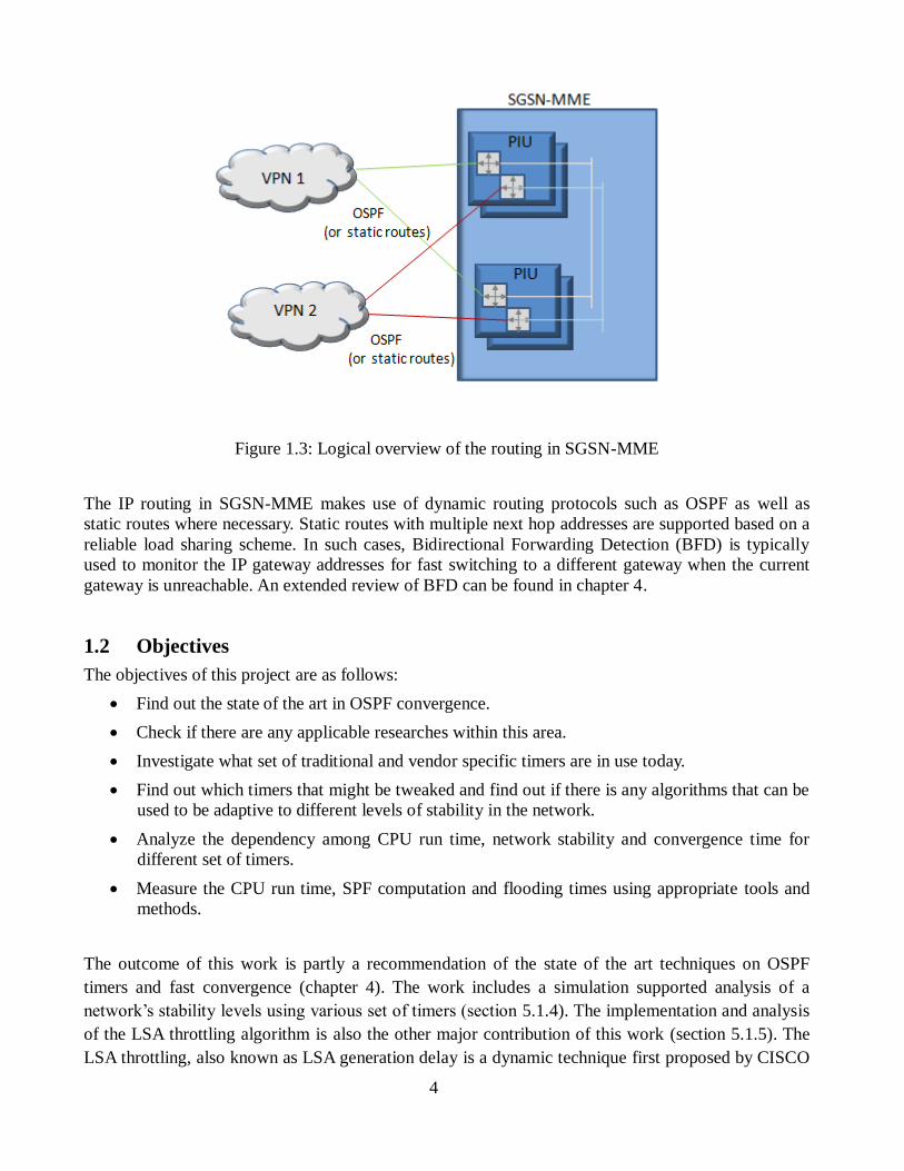
trusted Virtual Private Networks (VPNs) for enhanced security. The figure below shows the routing

in SGSN-MME from a logical perspective with two VPNs each with alternative (redundant) routing

paths. The SGSN-MME architecture allows the same VPN to be configured over multiple Protocol

Interface Units (PIUs) using the same IP address for load sharing purpose and also a single PIU can

run multiple VPNs separated by VLANs.

4

Figure 1.3: Logical overview of the routing in SGSN-MME

The IP routing in SGSN-MME makes use of dynamic routing protocols such as OSPF as well as

static routes where necessary. Static routes with multiple next hop addresses are supported based on a

reliable load sharing scheme. In such cases, Bidirectional Forwarding Detection (BFD) is typically

used to monitor the IP gateway addresses for fast switching to a different gateway when the current

gateway is unreachable. An extended review of BFD can be found in chapter 4.

1.2 Objectives

The objectives of this project are as follows:

Find out the state of the art in OSPF convergence.

Check if there are any applicable researches within this area.

Investigate what set of traditional and vendor specific timers are in use today.

Find out which timers that might be tweaked and find out if there is any algorithms that can be

used to be adaptive to different levels of stability in the network.

Analyze the dependency among CPU run time, network stability and convergence time for

different set of timers.

Measure the CPU run time, SPF computation and flooding times using appropriate tools and

methods.

The outcome of this work is partly a recommendation of the state of the art techniques on OSPF

timers and fast convergence (chapter 4). The work includes a simulation supported analysis of a

network’s stability levels using various set of timers (section 5.1.4). The implementation and analysis

of the LSA throttling algorithm is also the other major contribution of this work (section 5.1.5). The

LSA throttling, also known as LSA generation delay is a dynamic technique first proposed by CISCO

5

Systems, Inc [12] to limit excessive and unwanted LSA generations at times of network instability.

The technique allows fast convergence taking the network’s stability into consideration. As part of the

implementation, this document also introduces a pseudo code of the LSA throttling feature. The

experiments and results from this work can be easily scaled up to any size OSPF network including

large scale ISP networks consisting of hundreds and thousands of routers.

1.3 Problem description

One of the strongest points of OSPF has traditionally been that it provides a network convergence

time in a couple of seconds. The convergence time is the time from a topology change until all other

nodes in the network recalculate their shortest path to all other nodes. The convergence time

determines how fast the routers adapt their routing tables to topological changes.

The demands on IP networks have risen over time since OSPFv2 was first introduced due to more

mission critical use of networks and due to the convergence of the telecom and IP networks. There is

now demand for sub-second convergence of OSPF networks. Recent advances in OSPF

implementation shows that this can be addressed through various tweaks of OSPF timers. But it’s not

enough to just decrease the different timers; the impact on network stability and on CPU cost has to

be analyzed as well.

1.4 Scope and Limitations

The simulation work and results in this thesis are done based on the application of OSPFv2 on point

to point links according to the RFC 2328. The discussions on fast convergence techniques mainly

focus on the standard as well as the newly introduced (vendor specific) timers. Optimization

techniques from traffic engineering (TE) extensions point of view are not part of this work. This

document doesn’t discuss details of OSPFv3 and/or its application on ipv6. OSPFv3 is discussed in

comparison with OSPFv2 on some points where we thought was worth mentioning.

The simulation tools used in this project were not readily provided by Ericsson. As part of the thesis,

we had to make a survey to choose a suitable tool from the open source domain, and that has required

us a considerable amount of time during the early phase of this project. After a thorough investigation

of the available choices, OPNET modeler 14.5(education version) and OMNET++ 2.2.1 were found

suitable for the work .A brief walkthrough of the selected tools is presented in chapter 5.

1.5 Related Work and Contribution

OSPF is a relatively matured and widely studied routing protocol. A lot of researches and publications

have been done on how to improve its convergence and stability aspects. Fast convergence deals with

boosting a network’s speed of information exchange to come to a consistent state whereas the stability

aspect assures the network won’t break while doing so.

Anindya B. John G. in [9] made an experimental study to find out the optimal hello timer for fast

convergence. Their simulation results on large ISP network consisting of 292 nodes and 765 links

shows that the hello interval can be safely reduced to 275 milliseconds for fast convergence without

impacting the network’s stability. The authors in [7] made a similar investigation on finding an

optimal value for static hello timers. They argue that it is unsafe to reduce the hello timer below 500

6

milliseconds but instead it’s possible to speed up the convergence by prioritizing the processing of

hello packets over the other types of OSPF messages. They also suggest the use of a set of

conservative approaches such as Packet Over SONET (POS) for fast failure detection, dynamic timer

usages for LSA generation and SPF computation as recommended fast convergence practices. On the

other hand, the authors in [8] and [36] proposed a dynamic mechanism to tune hello timer based on

the experienced congestion level. The technique in [8], also explained in chapter 3, works in such a

way that an OSPF peer increases its hello interval exponentially whenever it experiences a loss of

hello messages for more than a given threshold. The other similar technique proposed in [36] instead

uses a scheme called Dynamic Router Dead Interval (RDI) where the RDI is dynamically adjusted

based on the hello drop rate computed over a certain period of time. Cisco Systems, Inc. has devised a

technique to dynamically adjust the interval between each LSA generations called the minLSAInterval

which is one of the OSPF timers that attributes the most for fast convergence. The technique is

discussed at high level in [12].

One of the main contributions of this project is to implement and evaluate this algorithm in an OSPF

network using 1 millisecond hello interval and 4 millisecond routerDeadInterval. The original plan

was to use sub second hello timers but that was impossible due to simulator limitations. As part of the

implementation, the paper also presents the pseudo code of the algorithm (section 5.1.5.6). The paper

also contains theoretical discussion of the state of the art techniques on OSPF fast convergence as

well as an experimental evaluation of the relationship between different sets of OSPF timers and

network stability issues.

1.6 Structure of the dissertation

This dissertation is organized as follows:

Chapter 2 discusses some of the topology change events in an OSPF network and the convergence

process following the change.

Chapter 3 presents OSPF fast convergence techniques.

Chapter 4 gives a mix of the different techniques to achieve sub-second convergence along with

similar experiences shared from literature review.

Chapter 5 discusses the work on the selected simulators and the analysis. It starts with a brief survey

of network simulators and advances further into the work done on the selected simulators.

Chapter 6 concludes the discussion by summarizing the main points related to OSPF sub-second

convergence.

Appendix 1 discusses the basics of OSPF.

7

2. OSPF Convergence Process

This chapter discusses the convergence process and the major factors affecting the convergence

process. Various types of topological changes as a cause for the convergence process are presented.

2.1 Routers Distributed Architecture

A router is a device that is responsible for forwarding packets between interconnected devices. A

routing protocol is a rule that governs how communications should be done between communicating

devices. Routers relate the IP header of a packet with the entries in their routing table to determine the

next best hop to forward the packet to. Modern routers have a distributed architecture that works

independently, the routing engine (control plane) and the packet forwarding engine (data plane). The

forwarding engine which is a switch fabric is used to forward between the inbound and out bound

interface of a line card. Therefore, the control plane takes care of the routing protocol and the data

plane takes care of the forwarding functions.

The control plane is responsible in constructing and maintaining the RIB from which the FIB is

constructed; the RIB consists of best paths to reach different nodes in a whole network [6]. The data

plane performs packet switching, route lookups, and packet forwarding. It basically sends out packets

from port to port based on a longest-prefix match and an access control list that filter out the packets.

The FIB contains the least required information to forward the IP packet, the next hop and the

associated outgoing interface.

.

Figure 2.1: The control and data planes

The forwarding process includes checking the IP headers and the TTL (Time to Live) of the incoming

packet, decrementing the TTL and updating the IP header checksum and look up the destination IP

address, in the FIB, to decide the next hop address. Routers perform SPF re-computation up on the

arrivals of LSA updates and the change is reflected on the forwarding table via the RIB. The

8

distributed nature of the router architecture reduces the load on the CPU. It can also allows the data

plane to keep forwarding packets to neighbors even when the control plane reboots for some activities

like updating its software.

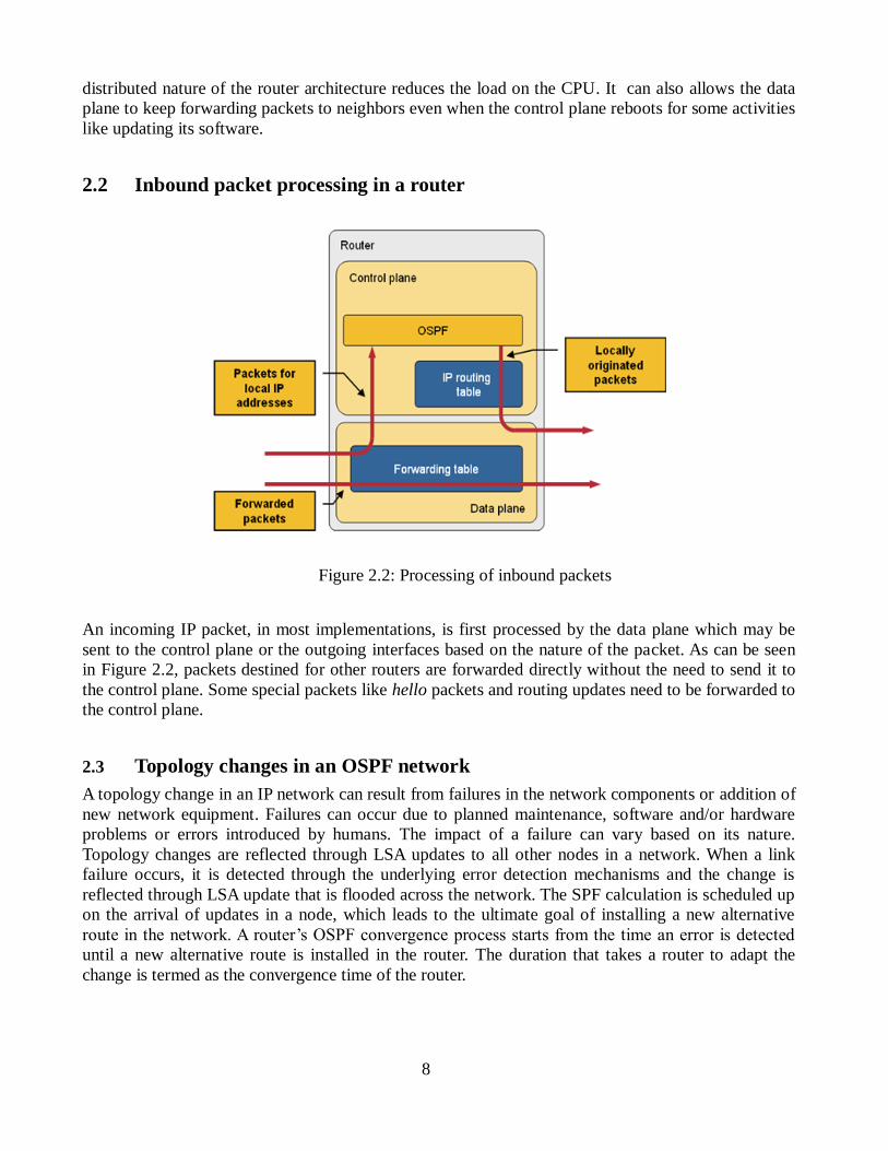
2.2 Inbound packet processing in a router

Figure 2.2: Processing of inbound packets

An incoming IP packet, in most implementations, is first processed by the data plane which may be

sent to the control plane or the outgoing interfaces based on the nature of the packet. As can be seen

in Figure 2.2, packets destined for other routers are forwarded directly without the need to send it to

the control plane. Some special packets like hello packets and routing updates need to be forwarded to

the control plane.

2.3 Topology changes in an OSPF network

A topology change in an IP network can result from failures in the network components or addition of

new network equipment. Failures can occur due to planned maintenance, software and/or hardware

problems or errors introduced by humans. The impact of a failure can vary based on its nature.

Topology changes are reflected through LSA updates to all other nodes in a network. When a link

failure occurs, it is detected through the underlying error detection mechanisms and the change is

reflected through LSA update that is flooded across the network. The SPF calculation is scheduled up

on the arrival of updates in a node, which leads to the ultimate goal of installing a new alternative

route in the network. A router’s OSPF convergence process starts from the time an error is detected

until a new alternative route is installed in the router. The duration that takes a router to adapt the

change is termed as the convergence time of the router.

9

2.4 Associated problems with OSPF convergence

Topology changes in a network are usually followed by one or more of the following issues until the

network adapts the change. Data packet losses or unordered deliveries, CPU/memory consumptions

due to extra packer processing and routing table calculations can be mentioned as examples. Such

excessive usage of resources, in the worst case might have the potential to meltdown the whole

network.

2.5 OSPF convergence process

OSPF is an interesting protocol since it involves a small time to install new route and re-route traffic

once a failure occurs. The OSPF convergence process is composed of the following processes.

Detecting changes in network status

Generating a new LSA to reflect the change

Flooding the LSA in the OSPF network

Performing SPF calculations on each router that receives the update information

Updating the RIB/FIB on each router

It is a requirement for all routers affected by topological changes to go through the process of

convergence and the time involved depends on how large and complex a network can be. In the

convergence process, the desirable effect is to achieve a faster convergence time. As routers converge

quickly it is relatively easy to avoid the problems mentioned in section 2.4.

2.6 Adding node to a converged network

Assuming a converged network in the first place Figure 3.3, adding a new router called New_node

results in the topology change of the network .As a result, the network is required to go through the

steps mentioned below so as to maintain a synchronized information about the network topology.

Figure 2.3: Adding router to a converged network

10

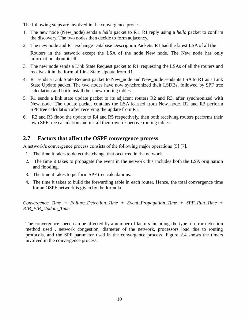
The following steps are involved in the convergence process.

1. The new node (New_node) sends a hello packet to R1. R1 reply using a hello packet to confirm

the discovery. The two nodes then decide to form adjacency.

2. The new node and R1 exchange Database Description Packets. R1 had the latest LSA of all the

Routers in the network except the LSA of the node New_node. The New_node has only

information about itself.

3. The new node sends a Link State Request packet to R1, requesting the LSAs of all the routers and

receives it in the form of Link State Update from R1.

4. R1 sends a Link State Request packet to New_node and New_node sends its LSA to R1 as a Link

State Update packet. The two nodes have now synchronized their LSDBs, followed by SPF tree

calculation and both install their new routing tables.

5. R1 sends a link state update packet to its adjacent routers R2 and R3, after synchronized with

New_node. The update packet contains the LSA learned from New_node. R2 and R3 perform

SPF tree calculation after receiving the update from R1.

6. R2 and R3 flood the update to R4 and R5 respectively, then both receiving routers performs their

own SPF tree calculation and install their own respective routing tables.

2.7 Factors that affect the OSPF convergence process

A network’s convergence process consists of the following major operations [5] [7].

1. The time it takes to detect the change that occurred in the network.

2. The time it takes to propagate the event in the network this includes both the LSA origination

and flooding.

3. The time it takes to perform SPF tree calculations.

4. The time it takes to build the forwarding table in each router. Hence, the total convergence time

for an OSPF network is given by the formula.

Convergence Time = Failure_Detection_Time + Event_Propagation_Time + SPF_Run_Time +

RIB_FIB_Update_Time

The convergence speed can be affected by a number of factors including the type of error detection

method used , network congestion, diameter of the network, processors load due to routing

protocols, and the SPF parameter used in the convergence process. Figure 2.4 shows the timers

involved in the convergence process.

11

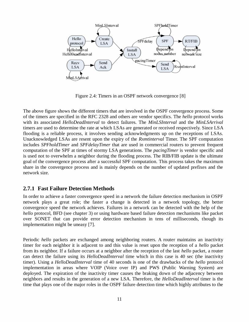
Figure 2.4: Timers in an OSPF network convergence [8]

The above figure shows the different timers that are involved in the OSPF convergence process. Some

of the timers are specified in the RFC 2328 and others are vendor specifics. The hello protocol works

with its associated HelloDeadInterval to detect failures. The MinLSInterval and the MinLSArrival

timers are used to determine the rate at which LSAs are generated or received respectively. Since LSA

flooding is a reliable process, it involves sending acknowledgments up on the receptions of LSAs.

Unacknowledged LSAs are resent upon the expiry of the Rxmtinterval Timer. The SPF computation

includes SPFholdTimer and SPFdelayTimer that are used in commercial routers to prevent frequent

computation of the SPF at times of stormy LSA generations. The pacingTimer is vendor specific and

is used not to overwhelm a neighbor during the flooding process. The RIB/FIB update is the ultimate

goal of the convergence process after a successful SPF computation. This process takes the maximum

share in the convergence process and is mainly depends on the number of updated prefixes and the

network size.

2.7.1 Fast Failure Detection Methods

In order to achieve a faster convergence speed in a network the failure detection mechanism in OSPF

network plays a great role; the faster a change is detected in a network topology, the better

convergence speed the network achieves. Failures in a network can be detected with the help of the

hello protocol, BFD (see chapter 3) or using hardware based failure detection mechanisms like packet

over SONET that can provide error detection mechanism in tens of milliseconds, though its

implementation might be uneasy [7].

Periodic hello packets are exchanged among neighboring routers. A router maintains an inactivity

timer for each neighbor it is adjacent to and this value is reset upon the reception of a hello packet

from its neighbor. If a failure occurs at a neighbor after the reception of the last hello packet, a router

can detect the failure using its HelloDeadInterval time which in this case is 40 sec (the inactivity

timer). Using a HelloDeadInterval time of 40 seconds is one of the drawbacks of the hello protocol

implementation in areas where VOIP (Voice over IP) and PWS (Public Warning System) are

deployed. The expiration of the inactivity timer causes the braking down of the adjacency between

neighbors and results in the generation of a new LSA. Therefore, the HelloDeadInterval timer is the

time that plays one of the major roles in the OSPF failure detection time which highly attributes to the

12

convergence speed. By reducing this timer to an optimal small value, the failure detection time can be

improved.

2.7.2 Event Propagation

In an OSPF network an LSA can be used to reflect the status of a network, a router LSA describes the

link states of a router in a network. Once a failure is detected in a network, propagating the change to

all routers in the network is another factor that affects the OSPF convergence speed. To control the

frequency of the LSAs generated up on changes in a network, RFC 2328 recommends that every two

LSAs should be sent within 5 seconds interval; the so called MinLSInterval .

The event propagation can be affected due network congestion that may be caused by LSA storms or

other timer effects associated with LSA generation and flooding. For a router affected by change to

generate an LSA, it relies on the time of the underlying error detection mechanism and the chosen

MinLSInterval value. The flooding process includes the delay that occurs at the receiving routers

which is the MinLSArrival value (the inter-packet arrival time) plus the pacingTimer applied by the

sending routers and the delay that may be introduced at the time of propagation. Depending on the

nature of the network, an LSA storm can result due to any of the following factors.

A flapping Link/router.

Fiber cuts resulting in one or more link failures

Software version change resulting in refresh of all LSAs in the system or

Due to the periodic, 1800-second, LSA refreshes time in the network.

The flooding scope of a topology change can vary depending on the type of the topology change that

occurred. A router, network and summary LSAs are flooded throughout a single area where as a new

AS External router LSA might be flooded to all the areas within an AS. Having a small MinLSInterval

value can help achieve fast convergence but keeping it to zero is not recommended as it highly affects

the routing stability and consumes resource. To balance the need for both convergence and the

stability of a network, different vendors like Cisco and Junipers have implemented exponential back

off algorithm for LSA generation called LSA throttling (see chapter 3 for details).

2.7.3 SPF Calculation

LSAs that reflect topological change are followed by a route table calculation and updating the FIB

on the line cards. In an OSPF network each node making itself as a root node, constructs the SPF tree

using the Dijkstra shortest path first algorithm. The Shortest path resulting from the SPF calculation is

the optimal shortest distance from a source to a destination. At the end of the SPF calculation the

optimal routes are populated in to the routing table and this result is reflected to the Forwarding

Information Base (FIB), depending on the router’s architecture. The SPF computation is the function

of the number of nodes in the network and the number of prefixes advertised.

Some implementations follow the traditional approach in which SPF is calculated on every new LSA

arrival which requires a high CPU utilization. To avoid a continuous route calculation and minimize

the router’s processor consumption, commercial routers introduce the SPFholdTimer and the SPF-

13

delayTimer (see Figure 2.4 above).The SPFholdTimer specifies the time gap between two consecutive

SPF calculations. The SPFdelayTimer specifies the time that a router should wait to perform the SPF

calculation after receiving the first LSA in an attempt to include more LSAs in to the calculation.

In a stable network, it is desirable to have the SPFholdTimer to be small to achieve fast convergence,

since there is not that much topological change that may occur in the network. In unstable network,

where there are frequent changes in the network topology, having a small value of SPFholdTimer

could result in a frequent SPF calculation. As a result, in such network large intervals in the SPF

calculation is preferable to accumulate several changes and execute them at once.

Both the SPFholdTimer and the SPFdelayTimer help achieve stability in a network but reduce the

speed in which a network converge to a new topology. The Cisco routers, after 12.2(14) version,

implements a simple exponential back-off timers to balance the need for fast convergence and

stability of a network under any circumstance. In order to optimize the routing table calculation

another alternative method of scheduling the route table calculation such as LSA correlation and iSPF

calculation methods have been suggested.

2.7.4 Routing Information Base (RIB)/ Forwarding Information Base (FIB)

Update

RIB also named as routing table, contains reachable information and the associated cost for each

route. Routes are installed either in static or dynamic way. To reflect changes in a topology OSPF

performs RIB updates following the SPF calculations. Depending on the type of router architecture

the RIB can be propagated further to the forwarding table.

The RIB contains the destination network ID, the costs associated with the interface and the next hop

address that is going to be used as a gateway to forward incoming packet. Forwarding information

Base is a copy of the routing table but it contains the least required information to forward an IP

packet. The FIB may not be required to track the whole paths and their corresponding metrics to

reach a network. The FIB is optimized for forwarding efficiency or for fast lookup of destination

addresses. When packet meant for other nodes arrive at some router the FIB tries to quickly forward

the packet to the next hop.

A successful SPF calculation is followed by the RIB/FIB update, which is the ultimate goal. The

update time is linearly dependent on the number of modified prefixes that can greatly affect the

convergence time of a network [8]. The impact can take a considerable amount of time in large

networks. To improve the update time some routers use a proprietary method called iFIB that reflects

only the changed part than to construct the FIB from a scratch.

14

3. OSPF Fast Convergence Techniques

As discussed in the previous chapters, it is generally possible to achieve fast convergence by setting

the timers to a lower value. However, it’s equally important to analyze the associated impact on

network resources (CPU, memory, bandwidth, etc.), especially on networks with frequent

instabilities. Knowing the optimal settings of these timers has always been a challenge for one reason

that it’s highly dependent on a number of generic factors including the network’s expected

traffic/congestion level, number of nodes/links and other physical link constraints.

This challenge has led to the evolution of what we call dynamic timers; timers that can change

adaptively with the experienced network behavior. Nowadays, most of the optimizations in OSPF lay

on the implementation of dynamic timers which can be preferably introduced at various operational

levels; starting from hello packet origination to LSA generation, Shortest Path First (SPF)

computation, flooding and FIB updates. This chapter assesses some of the state of the art techniques

on the use of dynamic timers and also a few other optimization techniques.

3.1 Dynamic Hello Timers

Hello timers are one of the integral components of many routing solutions. They help discover

neighbors and detect failures. The OSPFv2 implementation based on RFC 2328 specifies a fixed hello

interval of 10 seconds which is quite large according to modern researches and experience [7] [9].

With the rapid increment of modern day routers computing power, it has now become a common

sense to lower the hello interval to a millisecond range. While it’s generally safe to do this on stable

networks, it might have some undesirable effects on unstable networks with frequent link/node flaps

and congestions. In these and similar situations where the CPU is kept busy, the hello timers may not

be timely processed and assumed to be lost (hello omission). The frequent omission of hellos makes

the neighbor relationship to go up and down and the neighboring routers to generate LSAs that reflect

this. This in turn forces all routers in the network to add and delete a particular route every now and

then, causing a network wide route flap and disruption. Therefore, In the presence of such flaps, an

implementation might prefer to temporarily break the communication between adjacent neighbors

over the unstable link in an attempt to discourage the availability of the route and avoid the resulting

route flap. Dynamic hellos are designed with that in mind; to suppress the route flaps caused by link

flaps in point to point OSPF networks.

The dynamic hello techniques, as detailed by the authors in [8] makes use of the hello_tune timer

assigned for each active interface. The router monitors the presence/absence of instabilities (route

flaps, in this case) within the hello tune interval. If, within the hello tune period, a routers experiences

a neighborDown event (due to the firing of the inactivity timer) more than a given threshold amount,

the router doubles its hello interval. In doing so, the router presumes the presence of a route flap due

to a link flap and the doubling of the hello interval causes a hello mismatch with its neighbor. As two

OSPF neighbors should have the same hello interval, this variation causes the neighbor relationship to

be temporarily suspended until the other neighbor also doubles its hello interval, which is more likely

to happen before the first router doubles its hello interval for the second time because the former has

a smaller routerDeadInterval . Once the other neighbor has doubled its hello interval, the adjacency

15

will recover once again with an increased routerDeadInterval this time. If the flap continues for the

next hello_tune interval, the router once again doubles its hello interval (exponential growth) and the

whole process continues once more. With the absence of such flaps within the hello_tune period, the

hello timer is reset to its default value. The main objective behind this technique is to avoid route

flaps by masking link flaps within the increased routerDeadInterval. The maximum threshold for the

hellos is set to 10 seconds and the initial value is set to 1 second in the experiment.

We have tried to illustrate one possible way of this technique in the following figure.

Figure 3.1: The Dynamic Hello Scheme.

Amir Siddiqi and Biswajit Nandy [36] have proposed a similar technique to mitigate route

instabilities by dynamically tuning the OSPF failure threshold at times of congestion. This technique

instead uses a fixed hello interval but varies the routerDeadInterval (RDI) based on the experienced

network congestion level. The congestion levels are determined by monitoring the history of the

number of hello packets received over a certain period of time and then determining the hello drop

rate based on which the RDI values are dynamically assigned. Network interfaces are classified as

master and slave based on their router ID .Only the master can changes the RDI value but the slave

can propose a change when it experiences congestion. Simulation results of this technique under a

highly congested network show a significant reduction in the number of adjacencies lost compared to

the standard OSPF implementation.

16

3.2 Bidirectional Forward Detection (BFD)

Failure detection time is one of the factors that delay the convergence process as discussed in the

chapter 2. In traditional OSPF implementations, this time is dictated by the routerDeadInterval

(4*hello). Achieving sub-second convergence using native hellos or fastHellos is challenging if not

impossible for a simple fact that even fastHellos do require a minimum of 1 second to detect failure

[10]. And on top of this, using fast hellos may not be a good choice for the operation highly consumes

CPU cycle. The best alternative for most of the IGP implementations today is BFD (RFC5880) which

is based on sub-second keep-alive timers. BFD is a light weight failure detection protocol designed to

detect fault quickly in the bidirectional path of two routers including the interfaces, data links, and

forwarding planes[7] [10]. It is designed to be implemented on the data plane of distributed router

architecture independently of media, data and routing protocols.

Unlike point to point links that have a hardware failure detection mechanism, layer 2 technologies

such as Ethernet that mainly rely on hello protocol to detect failures require fast failure detection

mechanisms like BFD. BFD in its best-scenario provides comparable failure detection time as the

expensive layer1/2 technologies such as packet over SONET/SDH which normally requires a few

tens of milliseconds [7] [10].

3.2.1 BFD Neighbor Relationship Formation and Tear Down

BFD relies on the configured routing protocol to discover its peer. As an OSPF process discovers a

neighbor, it sends a request to the BFD running locally to form a BFD neighbor relationship with the

neighbor. BFD neighbors create BFD session and negotiate the time in which the control packets are

sent and received to detect connectivity problems.

Figure 3.2: BFD neighbor relationship formation (Asynchronous mode)

Figure 3.3: BFD Error Detection Mechanism (Asynchronous mode)

When failures occur in a network as shown in Figure 3.3, control packets are not received on both

sides. As a result, the BFD session is torn down and the BFD reports to the OSPF that the neighbor is

unreachable. This helps the OSPF to detect failures quickly and find an alternative path if available.

17

Two main modes of operation are supported by BFD, asynchronous and demand modes. The

asynchronous mode is the main mode of operation that involves a periodic exchange of control

packets (just like hellos). Most of Cisco’s IOS systems support asynchronous mode BFD. The

demand mode that works over demand circuit like ISDN does not involve a periodic exchange of

BFD control packets after the BFD session is established. A short sequence of BFD packets is

exchanged instead when a device needs to check connectivity explicitly and it can operate

independently in each or both directions [11] [7]. BFD also support echo function that works with

both asynchronous and demand modes. The echo function allows a device to send echo packet to its

neighbor by setting its own address as the destination address (self-destined packets); the neighbor

immediately forwards the echo packet without processing it and this reduces the round-trip time jitter.

BFD echo packets are encapsulated in UDP packet and destination port 3785 and detect failures

between directly connected neighbors. If the echo packets sent are not received within the BFD

detection time interval then the device can declare that session is over. Since Echo function can

independently provide a faster detection mechanism, the rate in which the BFD control packets are

exchanged between devices can be reduced. The disadvantage of BFD is that it cannot detect failures

on control plane as it is implemented on the data plane .However, it can be used with fast hellos to

achieve that. Details about the BFD protocol can be found on RFC 5880.

3.3 Fine-Tuning Delays in LSA generation, SPF computation and Flooding

This section discusses various optimization techniques for LSA generations, SPF computations and

Flooding.

3.3.1 LSA Throttling (dynamic minLSAInterval)

The implementation details of this technique, as part of our project, are discussed in chapter 5. Here

we will brief how the technique works. Topology changes in an OSPF network are communicated

using LSAs. RFC 2328 mentions the following topological changes as possible causes of LSA

origination.

An Interface's state changes(Up/Down)

Designated Router(DR) changes(Broadcast, NBMA networks)

Neighboring routers change to/from FULL state

In general, a change in any of the contents of an existing LSA results in a new LSA that reflects the

new change. For safety reasons, the origination of any two consecutive LSAs should be at least

minLSAInterval apart. MinLSAInterval (default 5s) is a router’s built in mechanism to safeguard the

router’s CPU at times of large scale topology changes or persistent link/node flaps. However, for

today’s modern CPUs, this delay seems too conservative and intolerable. Instead, as argued in [7], it

can be set to a smaller initial value for fast convergence to changes and made to adaptively increase

with the network load. LSA throttling is one such approach to adaptively increase/decrease the LSA

origination interval using exponential back off algorithm. It was introduced in Cisco IOS Release

12.2(27) SBC and documented in [12].

LSA Throttling makes use of initial interval, hold, and max_wait timers. If an LSA is to be generated

for any of the above reasons, it will be first delayed for an initial amount of time, and when the initial

delay timer expires, the hold timer starts with a given hold interval. Any subsequent events within the

hold interval will not generate an LSA; instead they are accumulated until the hold time expires and a

18

single LSA is generated as a result. And, so long as the flap continues, the process also continues

increasing the hold interval exponentially (2^t*hold) until it reaches a certain preset max_wait value.

The hold time will no longer increase beyond the max-wait but maintain that value even if the flap

continues. When no flap is detected within the duration of 2*max-wait delay, the hold timer is reset to

its initial value. It’s important to note that the hold interval should roughly equate to the total

convergence time explained in chapter 2 so that all routers would have already reflected the new

change before the next comes. Cisco’s default configuration uses 10 100 5000 milliseconds for these

three timers respectively and recommends that the hold interval should be set greater than or equal to

minLSArrival so that other routers receiving the update do not miss/drop valid LSAs.

3.3.2 SPF Throttling/SPF hold-down

Unlike modern high speed routers that take in the order of milliseconds to a few seconds to complete

SPF computation [13] [14], older systems of the 1980s and 90s took tens of seconds to complete the

operation. One factor for this, apart from the then smaller CPU power is the inefficiency of the

original dijikstra's algorithm. The original dijikistra's algorithm with an average complexity of nlogn

(even n2 for full mesh) is considered to be inefficient and less scalable in light of its modern variants

that take an average complexity of logn [15]. However, for modern ISP networks that maintain

hundreds of thousands of routes, SPF calculation has remained one of the CPU-intensive operations

that need to be optimized.

RFC 2328 specifies SPF computation immediately following the reception/origination of a new LSA

i.e., it was pure LSA-driven. If a router is scheduling SPF computation for every single LSA it

receives, that might ultimately locks the CPU only for SPF computation and all other useful tasks

would be stranded. A somewhat conservative approach of this uses a fixedHoldTime [16][17]

between successive SPF computations, but that too doesn't scale well and delays convergence. SPF

throttling is a modern SPF scheduling scheme that uses the same technique and procedure as LSA

throttling but it works on delaying the SPF computation after the LSA has already been

originated/received via flooding.

Three parameters namely spf-start interval, spf-hold timer and spf-max-wait timer are used in this

technique. The spf-hold controls the number of SPF iteration and it should be set optimal to the

convergence of the network. Likewise, spf-start should be kept as minimum as possible to allow for

instant reaction to changes like transient faults and occasional topology changes but large enough to

allow for successful flooding of the originated/received LSA before SPF starts.

Juniper's implementation of this differs a little in that it has two modes of operation namely slow

mode and fast mode, and unlike Cisco's exponentially increasing hold period it uses a linear

increment. If the number of SPF runs exceeds a preset limit called rapid runs within a certain check

period; the SPF computation switches to slow mode starting the hold-down timer. All subsequent SPF

events within the hold-down timer won't trigger SPF computation until the hold-down timer expires.

The following figure illustrates Cisco's implementation of SPF throttling which recommends 10 100

500 ms. A similar pattern can be inferred for LSA throttling as well.

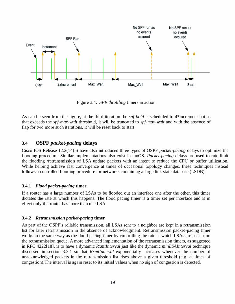
19

Figure 3.4: SPF throttling timers in action

As can be seen from the figure, at the third iteration the spf-hold is scheduled to 4*increment but as

that exceeds the spf-max-wait threshold, it will be truncated to spf-max-wait and with the absence of

flap for two more such iterations, it will be reset back to start.

3.4 OSPF packet-pacing delays

Cisco IOS Release 12.2(14) S have also introduced three types of OSPF packet-pacing delays to optimize the

flooding procedure. Similar implementations also exist in junOS. Packet-pacing delays are used to rate limit

the flooding /retransmission of LSA update packets with an intent to reduce the CPU or buffer utilization.

While helping achieve fast convergence at times of occasional topology changes, these techniques instead

follows a controlled flooding procedure for networks containing a large link state database (LSDB).

3.4.1 Flood packet-pacing timer

If a router has a large number of LSAs to be flooded out an interface one after the other, this timer

dictates the rate at which this happens. The flood pacing timer is a timer set per interface and is in

effect only if a router has more than one LSA.

3.4.2 Retransmission packet-pacing timer

As part of the OSPF’s reliable transmission, all LSAs sent to a neighbor are kept in a retransmission

list for later retransmission in the absence of acknowledgment. Retransmission packet-pacing timer

works in the same way as the flood pacing timer by controlling the rate at which LSAs are sent from

the retransmission queue. A more advanced implementation of the retransmission timers, as suggested

in RFC 4222[18], is to have a dynamic RxmtInterval just like the dynamic minLSAInterval technique

discussed in section 3.3.1 so that RxmtInterval exponentially increases whenever the number of

unacknowledged packets in the retransmission list rises above a given threshold (e.g. at times of

congestion).The interval is again reset to its initial values when no sign of congestion is detected.

20

3.4.3 Group packet-pacing timer

Prior to this feature, Cisco’s OSPF implementation [19] used to have a fixed 30 minute refresh

interval after which all the self-generated LSAs of a router are refreshed. The refresh applies to all

such LSAs at a time despite their current respective ages. Such a schedule creates a periodic spike of

LSAs flooded to the network and that would require a considerable amount of CPU processing and

buffer utilization.

The OSPFv2 specification according to RFC 2328 instead applies an individual refresh time for each

self-generated LSAs so that an LSA is flooded when it hits its 30 minute limit (which is its half-age).

This on the other hand makes the flooding more frequent and inconvenient. A more recent

implementation of Cisco adds a delay called group pacing delay (default 240ms) to each refresh times

in an attempt to contain several LSAs into a single LSA update packet. This would make the flooding

more efficient and reduce the load on the sender as well as on the receiving neighbors, but this

somehow delays the convergence process. Details can be found in [7] [20].

3.5 IP Event Dampening

IP event Dampening or BGP dampening (for BGP, rfc2439) is also a widely used technique to ensure

global routing stability by reducing the effect of route flaps which are caused by high-frequency

interface/link flaps. Almost all routing solutions of Cisco [21] since IOS release 12.0(22) S and

junOS’s BGP implementation [22] include this feature in their distributions. We will brief Cisco's

implementation of this below.

Cisco's IGP implementation of this is used to punish a persistently flapping interface by hiding its

state transitions(UP/Down) from upper layer protocols and hence from the network. This helps to

temporarily shut down the link and freeze all routes through it until it stabilizes. This technique is

very similar in effect with LSA throttling but is a bit conservative and may not be enabled if a router

is already using LSA throttling or the other way round. Every time an interface flaps (goes down), it

is assigned a penalty value according to the formula Pn =Pn-1*2^ (-t/H) +Pn-1. If this accumulated

penalty value exceeds a maximum threshold value called the suppress threshold, the interface is

suppressed. It’ll be unsuppressed when the penalty drops below the re-use value.

Figure 3.5: IP Event Dampening [21]

21

The algorithm makes use of the five parameters; penalty (figure of merit as junOS calls it),

suppress/cut-off threshold, half-life period, reuses threshold and max- suppress time. The explanation

follows the definitions of these parameters.

Suppress threshold (default 2000) - Is the maximum accumulated penalty value after which the link

is suppressed. If the penalty counter is >1 in the half-life period, the penalty keeps on increasing by

P*2^ (-t/H) + P.

With the absence of flap in every half-life period, the penalty follows exponential decay according to

the formula P(t)=P(0)*2^(-t/H); whereas if the flap counter is >1 in the half-life period ,the penalty

keeps on increasing by P*2^(-t/H)+P .

P (t) stands for the penalty (initially 1000) at time t and H for the half-life period defined below.

Half-life period (5s) - Is the duration of time after which the penalty is exponentially decayed

according to the above formula (determines how fast the penalty decreases exponentially).This time

has to be carefully chosen based on the frequency of the flap. Generally, the derivation from the

above formula holds H >= T/log2 (P/(S-P).

Reuse Threshold (default 1000) - Is the lower limit of penalty. If the penalty value falls below this

value, the interface is unsuppressed/ reused.

Max-suppress-time (default 4*half-life) - Refers to the maximum time a route can be suppressed. It’s

recommended to have this feature deployed specially on networks with redundant links, which are

typical of large service providers, due to the fact that routers start to use an alternative link stably unt il

the flapping link settles.

3.6 SPF enhancements

3.6.1 Incremental SPF (iSPF)

SPF computation using the old Dijkstra's algorithm, aka static dijkistra [23] is now believed to be

inefficient in many aspects. One of these limitations is that a full SPF computation is undergone over

all LSAs in the LSDB for every new LSA received. Nevertheless, it may be the case that such an LSA

won’t affect/change the existing Shortest Path Tree (SPT) tree or it may only changes part of it.

This happens for example, when the LSA describes the failure of a link which is not part of the saved

SPT (every new SPT has to be saved for iSPF). Such topology changes should simply be ignored if

identified properly.

iSPF is a more sophisticated approach that avoids such unnecessary computations by carefully

examining the newly arriving LSAs against the saved SPT before triggering a new SPF. iSPF also

enables fast RIB updates [23] by avoiding redundant RIB updates and this contributes a lot for the

convergence speed.

The feature is available in Cisco IOS Release 12.0(24) S and later. Please refer the description

following figure 3.6 for this and some more properties of iSPF.

22

Figure 3.6: Sample Topology (left) and spanning tree (right)

property1. If the topology change is the addition of new leaf node like node R8 in the fig above,

simply extend the SPT from R6 and its cost would be the cost to R6 plus the interface output cost to

R8. This property is similar to the partial route computation discussed in section 3.6.2.

Property2. If a link that wasn't previously in the saved SPT, say R4-R5 is down, and then this

wouldn't trigger a new SPF.

Property3. If any link in the current SPT tree fails say the link between R1 and R5, then that would

trigger an SPF computation from the root to R5, R6, R7 and R8; that is to all the nodes in the sub tree

of the failed link.

iSPF proves more effective on topologies with fewer number of interconnections (less dense) and the

farther away the failure is from the root ,the simpler would the computation be and this compensates

for the longer propagation delay resulting from such distant failures.

3.6.2 Partial Route Computation (PRC) in ISIS

As pointed in the previous section, OSPFv2's inherent way of handling information in its LSAs has

some inconvenience when it comes to PRC. IP prefix information (the connected subnet information)

is an integral part of an OSPF type 1 or type 2 LSAs which also carries topology information. So

whenever an IP prefix or the status of a stub link changes in the area, the same LSAs are generated

like for any other topology change that must trigger SPF. OSPF has no way to identify that such

changes are only of IP prefix and not of topology, as a result of which it schedules a normal full SPF.

Should it detect such changes, only PRC over the changed prefixes will be computed which is way far

simpler task to do. But OSPF does so only for type3 and type5 LSAs both of which carry IP prefix

information for external routes.

23

PRC is an integral part of ISIS due to the fact that ISIS’s handling of information in its LSP is more

suited to such optimizations. It has a separate TLV (Type-Length-Value) to carry the IP reachability

information and another one for IS (Intermediate System) Neighbors information (i.e. topology

information) out of which the SPF is computed independent of IP prefix information. Every IP

network in ISIS is considered as external and end up being a leaf; so whenever a stub link or a leaf

node is added/removed, ISIS does PRC just like a distance vector addition/removal and only transient

link failures that might potentially affect the whole topology do trigger a full SPT. That said, major

vendors like Cisco have managed to find a way out to this problem in OSPFv2 also, in such a way

when leaf nodes are added/removed from the network, the routes are redistributed just like type3 or

type5 LSAs instead of the normal case where they are advertised as type 1/2 LSAs. This trick has

enabled OSPF to do PRC on stub/leaf links, with a little more associated CPU overhead. However

with the introduction of iSPF to both OSPF and IS-IS this is no longer an issue. Please consult [18]

for more and associated issues on this and [25] for more explanation and difference between OSPF

and ISIS.

3.6.3 Partial Route Computation (PRC) in OSPFv3

OSPFv3 for IPv6 does this in a more smarter way by introducing a new type 9 LSA called an intra-

area prefix LSA that carries a separate intra-area network prefix information[26] (with no IP

addressing semantics). Router /Network LSAs are carried in separate LSAs that carry only topology

information.

In OSPFv3, LSA identifiers such as router Ids, Area Ids and Link-state Ids are all 32 bit numbers

written in dotted decimal representation but they are not actually IPv4 addresses but just numbers.

These numbers uniquely identifies each router in a given area; unlike OSPFv2 which identifies

neighbors by their interface IP addresses (BR and NBMA networks) or an IPV4 router Ids (point to

point and other).

Type1 or Type2 LSAs do not carry IP addressing semantics information and are only transmitted

when information pertinent to SPF calculation exists. Otherwise simple IP prefix or stub link changes

only generate intra-area-prefix LSAs for which SPF would not run. This has made it easy to modify

IP prefix information without affecting SPT tree. Consult OSPFv3 RFC 5340[26].

3.7 LSA Correlation

LSA correlation is another SPF optimization technique proposed by the authors in [27].The authors

believe that the hold-time based SPF calculation that uses fixed/exponential back off algorithm has

unnecessary delays and is inefficient in some circumstances. They argue that individual LSAs are

only symptoms of a topology change and should not always trigger SPF computation. Instead, each

received link states in the update packets need to be collected over a period of time and correlated for

possible topology changes. The correlation process identifies possible similarities between link states

over adjacencies by thoroughly inspecting mainly the link ID, link Data, and link Type fields of the

LSA. And if any topology change is noticed during the correlation process that will immediately

trigger SPF calculation. The idea seems smart on one hand due to the fact that LSAs describing the

same change could be generated by multiple routers adjacent to each other, each of which possibly

requiring SPF runs when received by a destination.

24

Part of the processing in LSA Correlation is of course already specified in RFC 2328 and the authors

have noted that. The RFC clearly states that every received LSA should be checked for changes

against the previously stored LSAs unless it is the first time it is received, and SPF computation is

scheduled if and only if there is a difference in topology. However, as to our observation and the

authors claim, the original OSPFv2 specification doesn't differentiate similarities over adjacencies.

In the simplest case, when a link between two adjacent routers in a point to point network fails, both

the routers generate an LSA describing the change. A router receiving these LSAs possibly over a

period of time may schedule SPF for each despite the fact that they talk about the same thing. To give

another example, suppose a central node that carries multiple adjacencies in point to point network

crashes, as a result of which each of the adjacent routers generate an LSA describing this. Suppose a

distant router receiving each of these LSAs. The traditional implementation might schedule SPF for

each LSA it receives. The question is can we make this smarter? The author’s claim this can be made

smarter if the receiving router could somehow analyzed the nature of the link states in these LSAs.

For the first received LSA, it immediately schedules SPF (to reflect changes immediately, considering

it as an occasional topology change) but if a second LSAs is received from a different router

announcing the loss of adjacency with the same central node , then this might be a sign that the

central router is going down, so it waits for a while before running SPF hoping to see more such

announcements from the remaining adjacent routers also(its assumed that the calculat ing router keeps

track of all adjacency information of a router through their router's LSAs) and once it makes sure that

it has got hold of all the LSAs from all adjacent routers ,it schedules an SPF (the second SPF) . This is

in contrary to the pure LSA driven /fixed hold-time or an exponential bakeoff scheme which requires

more SPF runs may be one for each such instance in the worst case. Further details including the

pseudo code are found in [27] [23].

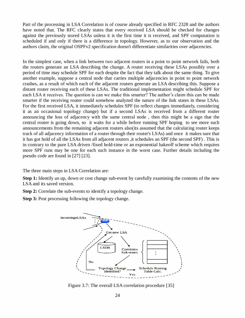
The three main steps in LSA Correlation are:

Step 1: Identify an up, down or cost change sub-event by carefully examining the contents of the new

LSA and its saved version.

Step 2: Correlate the sub-events to identify a topology change.

Step 3: Post processing following the topology change.

Figure 3.7: The overall LSA correlation procedure [35]

25

3.8 Graceful Restart (supported by both Cisco IOS and JunOS )

At times, it may necessitate that a router be down temporarily as part of a planned

maintenance/upgrade activity or due to unplanned events such as power cut or crash. Nevertheless, an

operator may still demand that the existing network communication should not be disrupted in the

meantime. This need can be addressed by a procedure called graceful restart or non-stop forwarding,

as documented in RFC 3623[28] [7]. Graceful restart makes use of the separate architecture of the

control and the data planes of modern routers. This distributed architecture has given a rise to the

possibility that the control plane, which takes care of all the OSPF operations, be restarted safely

leaving the data forwarding operation to the forwarding plane/data Plane. The procedure goes as

follows.

The restarting router called the initiating router sends a special message called grace LSA which is a

link local Opaque LSA to all its adjacent neighbors called helpers before it restarts (it does so after it

restarted before sending hellos, for unplanned reboots). The grace LSA is not to be flooded by the

helpers but is just a signal that the initiator is restarting so that the helpers should not break their

adjacency but instead pretend that the router is still up and continue advertising it in their LSA. The

initiator has to flush the grace LSA after a successful restart. In the meantime, the helpers enter in to a

helping mode.

In order to avoid possible mismatch, the initiating router saves its sequence number in a non-volatile

memory before it restarts and when it restarts, it re-introduces itself by re-originating its

router/network LSA, re-rerunning SPF and updating its forwarding table (it has to flush the grace

LSA before this). However, should any topology change occur during the restart period, the initiator

couldn't reflect this change in its forwarding table and that may potentially create a routing loop. In

such cases, its helpers would no longer hide its restart and break their adjacency (exit the helping

mode) by omitting the adjacent link from their LSAs. This time, both the initiator and its helpers

assume a normal restart and this is of course unwanted. For planned reboots, the network

administrator has to issue the appropriate command along with an estimated grace period which

should normally be less than 1800s (in order to avoid the LSAs being aged out during the restart

period). Graceful restart is not recommend at times of unplanned reboots due to that fact that the

router would not have enough time to prepare for it and this option should normally be disabled by

default, more on the RFC [28].

3.9 Incremental FIB Updates

FIB update times vary between routers depending on the nature of the failure and depending on the

number of routing prefixes affected by the failure. As experimental results show in [14] [13], FIB

update time contributes the most to the convergence delay. Recent improvements [29] suggest a

technique called incremental FIB update (iFIB). This technique, instead of dumping the whole routing

table on the line cards whenever a topology changes, it rather selectively updates only the routes or

the prefixes affected by the change. This approach works best with iSPF technique discussed in

section 3.6.1 and is proved to significantly reduce the convergence time as well as saves bandwidth.

26

4. Sub-second convergence and the associated challenges

OSPF has a better convergence time than a distance vector routing protocol like RIP. As mentioned in

chapter 3, a convergence speed can be affected by different factors. Today there is a high demand for

a sub-second convergence speed in a network, but the associated challenges of CPU utilization and

the network instability that can result need to be addressed as well. It is common to see 10 gigabit link

between two devices in core networks of services providers’. The failure of such links for a few

seconds can result in loss of information before the network fully converges, and it can impact

customers’ service. Here are some of the main reasons why sub-second convergence is very crucial.

The high importance of services uptime

The wide spread deployment of real time applications such as VOIP

Deployment of PWS like the Earthquake and Tsunami warning system (ETWS) as well as

Real-time mission and critical applications, from controls that are being used in industry to

different sophisticated battlefield communication systems.

As mentioned in chapter 2, network convergence time is the sum of the durations that takes to detect

failures, propagate the event, perform SPF calculation and update the RIB/FIB on each router. To

achieve a sub-second convergence, each step involved in the convergence process need to be

completed in milliseconds. Fast reaction to a perturbed network environments can lead to a network

that will not converge for certain period of time. While trying to achieve fast convergence, network

instability can be introduced on the other hand. Depending on how frequent the network component’s

status flaps, an excessive reaction by the underlying network’s protocol in some troubled environment

can consume high CPU and bandwidth, which even can have the potential to melt down the whole

network. As a result, stability is a key property of a recovery mechanism that needs to be addressed in

fast convergence.

In disturbed environments stability of a network can be maintained through controlling the way a

network recovery mechanism reacts up on changes. Dampening techniques that can be implemented

at different layers in a network are the basic methods to maintain stability in perturbed network

conditions. Interface dampening using an exponential decay algorithm and exponential back-off

algorithm both in LSA generation and SPF computations are some of the important techniques

available. Large convergence time, high routing load on routers and many route flaps within short

period of times can be taken as indicators for instability in a network.

4.1 Suggested methods to achieve fast failure detection mechanisms

As mentioned in the previous chapters, fast convergence is achieved through a quick discovery of

failures in a network. Sub-second error detection mechanism is one of the requirements to achieve

sub-second convergence. A quick discovery of failures in a network can be achieved using a reduced

hello timer, or more preferably using hardware based techniques and BFD.

27

A). A reduced hello timer

A reduced hello timer, reducing the hello timer notably improves the time to detect failures between

nodes, but it will also increase the load on every router as they are required to process the fast hello

packets. It is possible to reduce the hello interval to millisecond ranges but the impact on CPU and

network stability need to be taken in to consideration. CPU utilization in routers can increase for the

following reasons.

As routers process hundreds of neighbors’ fastHello packets

As multiple concurrent failures and/or recoveries occurs

As LSA storms occurs in a network and so on.

As OSPF reacts quickly to a continuous flaps in network that are close in time, several routes on a

routing table can be removed and added back within a short period of time, this is characterized as

route flaps. Route flaps caused by link flaps, in a perturbed OSPF network, always lead to a network

instability and unreliability [8]. Using a real ISP network model (292 nodes and 765 links) Anindya

Basu and Jon G. Riecke [9] observed a six-fold increase in the number of route flaps when reducing

the hello timer from 500 ms to 250 ms. They suggested the value 275ms as the optimal one. The

authors in [7] however suggest 500 ms as the optimal hello timer value with its failure detection time

capability of around 2 seconds.

In [15] it is stated that the hello timer is dependent on the physical constraint of links, like the link

noise hits. The authors in [30] tried to determine the optimal hello interval for a network. They

suggested that the optimal hello timer depends on the network’s expected congestion level and the

number of links in the network topology [30]; the authors in [7] also agree with these suggestions and

point out the network’s tolerance for false alarm as an additional factor.

The authors in [8] showed in their simulation network that fast detection, using an optimal hello

timer, is achievable under stable network. However, under unstable condition the dynamic hello timer

(see chapter 3) grows exponentially affecting the detection time and convergence speed but relatively

reducing the consumption of the CPU and bandwidth. It provides a more tolerant mechanism to

frequent network changes.

B). Hardware based techniques

Hardware based techniques can discover failures in tens of milliseconds but it may not be always

available either due to the network type or the cost involved. A point to point gigabit link can detect

failures between two nodes almost instantly, using a network pulse.

C). BFD

BFD in its best-scenario can help achieve 50ms error detection mechanism [7]. To detect failures in

forwarding planes, BFD is preferable over sub-second hellos both in terms of its quick detection and

its routing load. It can be used in conjunction with fastHello to minimize detection time in control

plane.

28

Finding an optimal hello timer that avoids false alarms and extra processing in a network is not an

easy task, as mentioned above. Quick failure detection mechanisms alone in a perturbed network

environments can lead to instabilities e.g. link flaps causing route flaps, and it can be prevented using

the dynamic hello timer techniques. The IP event dampening techniques(see chapter 3) can also be

used to damp some oscillating router interfaces in order to achieve a more stable system. Therefore,

BFD can be used with the IP event dampening techniques to restrain any possible flapping interfaces.

4.2 OSPF enhancements to optimize event propagation

Being one of the factors that determine the convergence process, the event propagation technique

requires an optimization to achieve fast convergence and at the same time a more stable network. The

event propagation can be affected due several factors, as mention in chapter 2. Among the factors, the

LSA storm results in high CPU and memory utilization at a router. This makes incoming packets to be

delayed or dropped, especially where fastHello is used. Packets being missed or delayed can result on

adjacency breakdown or an increase in the LSA retransmission rate that further can put the network to

unstable state.

In [18] the current “Best Current Practices” for OSPFv2 fast convergence are discussed. The

following methods have been stated as good practices to improve the scalability and stability of large

OSPF networks:-

1. Assigning high priority to hello packets and link state acknowledgment packets and low priority

to the others.

2. Reset the inactivity timers for an adjacency upon receiving any OSPF unicast packets or packets

sent to AllSPFRouters over point-to-point link instead of waiting for the hello packet only.

Adjacency is declared down only on the absences of these packets over the period of

RouterDeadInterval.

3. Use an exponential back-off algorithm to determine the rate at which the LSA be retransmitted

(RxmtInterval).This helps in reducing the rate of LSA retransmission as network experience

congestion.

4. Implicit Congestion Detection of neighbor routers and taking action using exponential back-off

mechanisms. The detection is done using the level of unacknowledged LSA packets. If the level

passes certain “high-water mark”, the rate at which LSAs are sent to the neighbor router is

reduced using exponential back off mechanism to some minimum rate. The rate is increased again

exponentially as number of unacknowledged LSAs to the router reaches certain “low-water

mark”. Both 3 and 4 helps avoid excessive congestion at a neighbor, the difference is that 3 is

only for retransmission but 4 works both for new and retransmission of LSAs.

5. Reducing the number of adjacencies to be brought up simultaneously, since sending large number

of adjacencies to neighbors can cause severe congestion due to database synchronizations and

LSA flooding activities. Here, only “n” number of adjacencies can be brought up at once. The

value”n”, which is configurable, is based on the processing capability of routers, total bandwidth

available for control plane traffic and propagation delay.

In addition to the different methods mentioned above, the following are some of the important

available enhancements that optimize the event propagation process in an OSPF network.

29

6. An LSA throttling technique that takes network convergence and stability into consideration (See

chapter.3).

7. Group pacing delay that is available in commercial routers, LSAs are grouped to refresh together

so as to reduce the number of LS update packets and prevent LSA storms (See, chapter 3).

8. Setting the DoNotAge bit in LSAs to avoid periodic refresh, this significantly reduce the LSA

processing overhead of routers [31]. Routers flood their self-originated LSAs with the DoNotAge

bit set, this reduce the protocol traffic overload in stable network. No need of re-flooding self-

originated LSAs every 30 minutes, the re-flooding interval is extended to configured forced-

flooding interval. New instances are originated up on LSA changes by the LSA originator.

4.3 Optimization in routing table calculations

Being one of the factors that determine the convergence process, routing table calculation requires an

optimization. Below are some of the important techniques that can be used to improve the routing

table calculation process.

Mechanisms Description Pros/cons

Fixed hold time It is a fixed delay that is enforced between

successive SPF calculations.

Prevent too many routing

table calculations after

topology change. Affect the

convergence duration but

good for routing stability.

SPF throttling,

with quite

period(Cisco)

Initially small hold time, but receiving one or

more LSAs within the period of hold time double

the next hold time until certain maximum value.

The hold time is reset to small value if no LSA is

received after 2*Max_hold , see chapter 3

Helps achieve fast

convergence duration. Tries

to keep the network stability

at times of network

disturbance that may result in

several SPF calculations.

Juniper scheme The first few SPF calculations are done with

small values (fast mode operation), if too many

SPF within certain threshold, it goes to large hold

time (slow mode). If no LSA is received during

the large hold time it is reset back to a small

value.

Changes with few routing

table calculation result in fast

convergence but affect the

frequency of the SPF

calculation for large scale

topology changes.

LSA correlation Tries to identify the underlying topology change

by correlating the LSAs.(See chapter 3)

Fast convergence with

reduced number of SPF

calculations.

iSPF Avoids unnecessary SPF computations by

examining newly arriving LSAs against the saved

SPT. (See chapter 3)

Contributes to convergence

speed, since it enables fast

RIB updates.

PRC Involves partial route calculations over changed

prefixes. (See chapter 3)

Improves the convergence

speed.

Table 4.1: Optimization in routing table calculations

30

4.4 Optimization in FIB updates

iFIB is used to optimize the FIB update time, it works best with iSPF (see chapter 3).

4.5 Achieving Sub-second convergence in large IP network

In [13] the authors have showed that it is possible to achieve sub-second convergence in large scale

network (Tier-1 ISP network model with 200 routers in Europe, America & Asia) without affecting

the stability of the network. Their simulation study was performed using ISIS, which equally applies

to OSPF. The simulation experiment contains the following assumptions and conservative approaches

Packet over SDH (Synchronous Digital Hierarchy/SONET (or POS) links in SP backbones or

BFD as means of sub second error detection mechanism.

Dynamic timers in LSA generation and SPF computations.

40 G link speed, no pacing timer

iSPF and iFIB

prefix prioritizations

Using the experience from this survey and the simulation experiment in this project, we believe that

using a combination of the following techniques at the different stages of the convergence process

enables to achieve a fast convergence without impacting the network stability.

Figure 4.1: Techniques to achieve fast convergence in OSPF

Dynamic RxmtInterval

& pacing delay

- Ip Evenet dampening

- LSA throttling

-Hardware Based/

BFD

Failure

Detection

Time

Event

propagaiton

SPF

calculation

RIB/FIB

Update

-iSPF

-PRC

DynamicHello/

Dynamic RDI

-iFIB

LSA Correlaiton/

SPF throttling

31

5. Simulations

This chapter starts with a brief overview of network simulation and then discusses the implementation

on the selected simulation.

5.1 Overview of Network Simulators

Before we started the simulation work, we had to make some survey to select a simulator suitable for

the implementation. Our targets were freely available tools with modifiable OSPFv2 source code and

also with a good GUI support. However finding one such ideal tool was difficult in the open source

world. The commercial tools we suggested were very expensive and there was no budget allocated to

buy one. NS3, OPNET IT Guru, QualNet, and OMNETPP, all of which are discrete event simulators

with C/C++ development environment were among the candidates. Ultimately, we managed to choose

OPNET Modeler Education version 14.5 simulator, one of the OPNET’s families of solutions for its

advanced GUI and support for simulation statistics related to many of the important properties of

OSPF such as convergence time. These advanced features are not available in OPNET IT Guru, the

other academic version by OPNET. We also used OMNET++ version 2.2.1 for its free and extendible

OSPFv2 source code using which we implemented the LSA generation delay feature. We will present

a brief overview of the candidate simulators followed by the experiments done on the selected tools.

Detail explanations can be found in the surveys [32] and [33].

5.1.1 Network Simulator-3 (NS-3)

NS-3 is a discrete-event network simulator/emulator widely used for educational and research

purposes. It’s a relatively new tool (first release 2008) designed to improve some of the inherent

limitations of NS-2 and other prior tools. It is not an update of NS-2 simulator although it makes use

of many of its models, nor is it backward compatibility with NS-2; it’s rather a different tool with an

entirely C++ development environment and an optional python support for scripting. NS-2 uses C++

for development but scripting must be done in OTcl (Object-oriented Tool command languages)

language. NS-3 provides a limited GUI support via NetAnim like NS-2 but newer tools such as PyViz

and NS3-Viz are also recent introductions. The drawback with this tool is that it doesn't have an

official OSPFv2 source code release but a user contributed one in the NS-3 experimental repositories

with lots of unresolved issues. We didn’t dare to use this tool due to such uncertainties and also due to

the complexity of NS-3 simulation environment added to the poor GUI support.

5.1.2 OPNET/QualNet

The other set of simulators we considered were products of OPNET (Optimized Network Engineering

Tools) Technologies and QualNet both of which are commercial closed source tools. The versions

shipped with the extendable source code are very expensive. QualNet doesn't have a free version and

we didn't need to investigate it further. OPNET solutions on the other hand have educational versions

one of which is OPNET IT Guru. IT Guru is mainly designed for small scale network simulations

with some limitations on simulation parameters such as the number of nodes. OPNET families are

best for their sophisticated data analysis features and nicely designed GUI. OPNET Modeler is

another educational tool by OPNET that we considered for our study. We will briefly describe

OPNET Modeler and discuss what we achieved on it below.

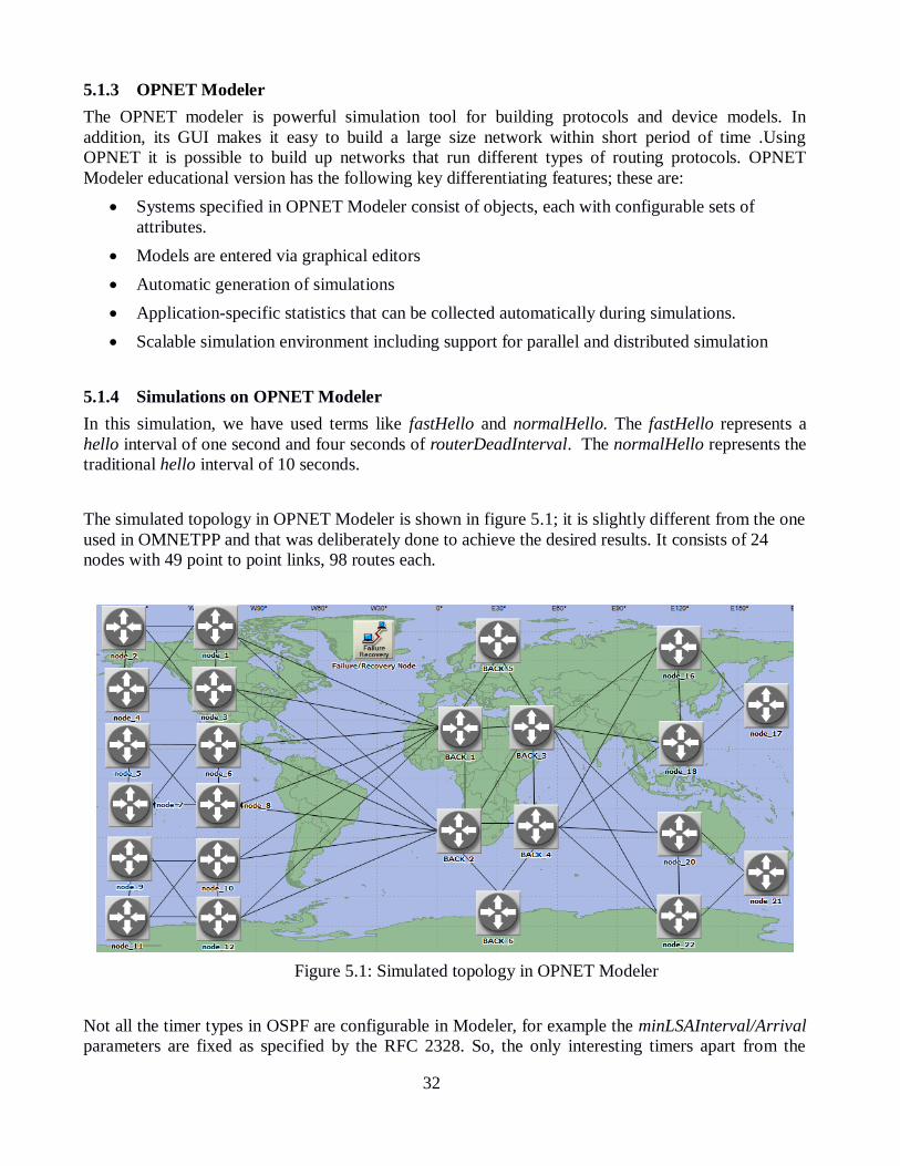
32

5.1.3 OPNET Modeler

The OPNET modeler is powerful simulation tool for building protocols and device models. In

addition, its GUI makes it easy to build a large size network within short period of time .Using

OPNET it is possible to build up networks that run different types of routing protocols. OPNET

Modeler educational version has the following key differentiating features; these are:

Systems specified in OPNET Modeler consist of objects, each with configurable sets of

attributes.

Models are entered via graphical editors

Automatic generation of simulations

Application-specific statistics that can be collected automatically during simulations.

Scalable simulation environment including support for parallel and distributed simulation

5.1.4 Simulations on OPNET Modeler

In this simulation, we have used terms like fastHello and normalHello. The fastHello represents a

hello interval of one second and four seconds of routerDeadInterval. The normalHello represents the

traditional hello interval of 10 seconds.

The simulated topology in OPNET Modeler is shown in figure 5.1; it is slightly different from the one

used in OMNETPP and that was deliberately done to achieve the desired results. It consists of 24

nodes with 49 point to point links, 98 routes each.

Figure 5.1: Simulated topology in OPNET Modeler

Not all the timer types in OSPF are configurable in Modeler, for example the minLSAInterval/Arrival

parameters are fixed as specified by the RFC 2328. So, the only interesting timers apart from the

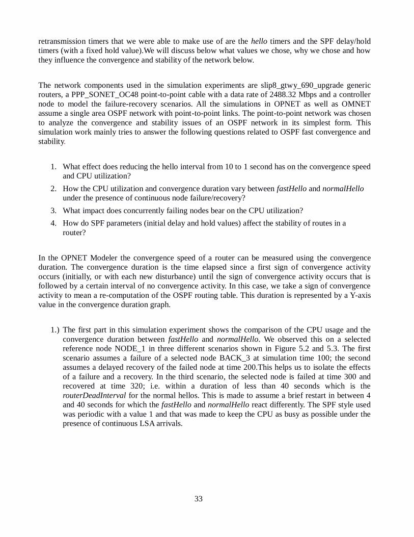
33

retransmission timers that we were able to make use of are the hello timers and the SPF delay/hold

timers (with a fixed hold value).We will discuss below what values we chose, why we chose and how

they influence the convergence and stability of the network below.

The network components used in the simulation experiments are slip8_gtwy_690_upgrade generic

routers, a PPP_SONET_OC48 point-to-point cable with a data rate of 2488.32 Mbps and a controller

node to model the failure-recovery scenarios. All the simulations in OPNET as well as OMNET

assume a single area OSPF network with point-to-point links. The point-to-point network was chosen

to analyze the convergence and stability issues of an OSPF network in its simplest form. This

simulation work mainly tries to answer the following questions related to OSPF fast convergence and

stability.

1. What effect does reducing the hello interval from 10 to 1 second has on the convergence speed

and CPU utilization?

2. How the CPU utilization and convergence duration vary between fastHello and normalHello

under the presence of continuous node failure/recovery?

3. What impact does concurrently failing nodes bear on the CPU utilization?

4. How do SPF parameters (initial delay and hold values) affect the stability of routes in a

router?

In the OPNET Modeler the convergence speed of a router can be measured using the convergence

duration. The convergence duration is the time elapsed since a first sign of convergence activity

occurs (initially, or with each new disturbance) until the sign of convergence activity occurs that is

followed by a certain interval of no convergence activity. In this case, we take a sign of convergence

activity to mean a re-computation of the OSPF routing table. This duration is represented by a Y-axis

value in the convergence duration graph.

1.) The first part in this simulation experiment shows the comparison of the CPU usage and the

convergence duration between fastHello and normalHello. We observed this on a selected

reference node NODE_1 in three different scenarios shown in Figure 5.2 and 5.3. The first

scenario assumes a failure of a selected node BACK_3 at simulation time 100; the second

assumes a delayed recovery of the failed node at time 200.This helps us to isolate the effects

of a failure and a recovery. In the third scenario, the selected node is failed at time 300 and

recovered at time 320; i.e. within a duration of less than 40 seconds which is the

routerDeadInterval for the normal hellos. This is made to assume a brief restart in between 4

and 40 seconds for which the fastHello and normalHello react differently. The SPF style used

was periodic with a value 1 and that was made to keep the CPU as busy as possible under the

presence of continuous LSA arrivals.

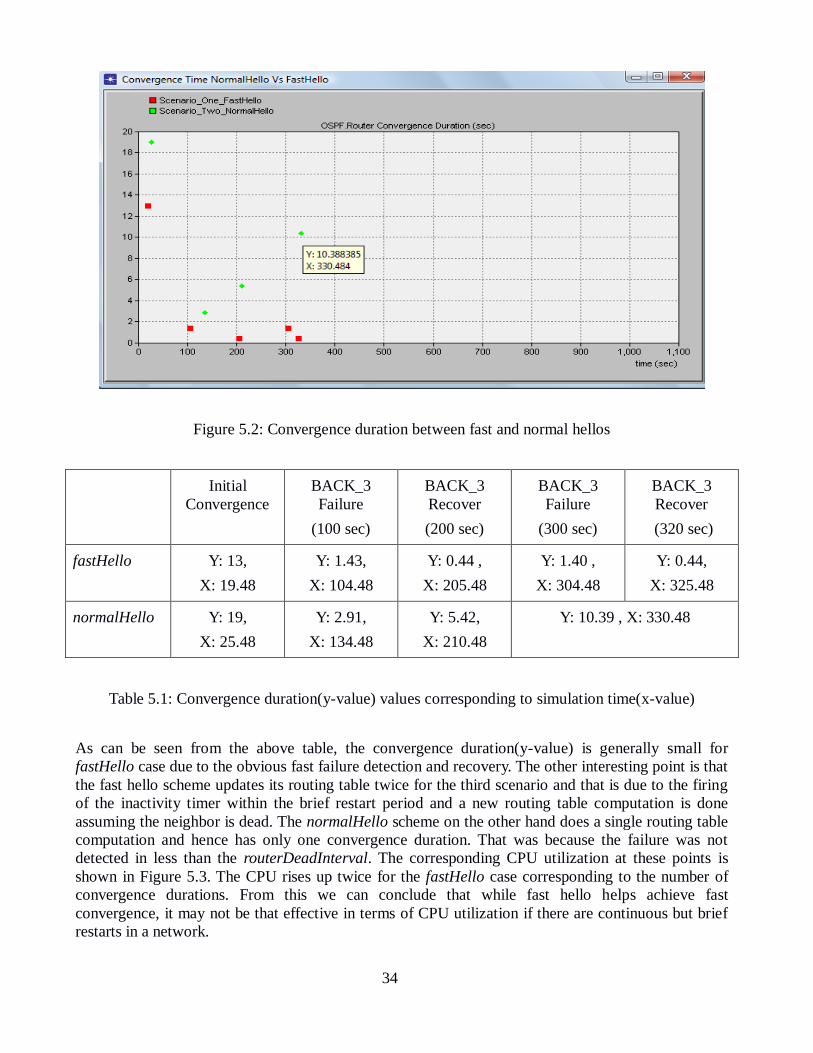
34

Figure 5.2: Convergence duration between fast and normal hellos

Initial

Convergence

BACK_3

Failure

(100 sec)

BACK_3

Recover

(200 sec)

BACK_3

Failure

(300 sec)

BACK_3

Recover

(320 sec)

fastHello Y: 13,

X: 19.48

Y: 1.43,

X: 104.48

Y: 0.44 ,

X: 205.48

Y: 1.40 ,

X: 304.48

Y: 0.44,

X: 325.48

normalHello Y: 19,

X: 25.48

Y: 2.91,

X: 134.48

Y: 5.42,

X: 210.48

Y: 10.39 , X: 330.48

Table 5.1: Convergence duration(y-value) values corresponding to simulation time(x-value)

As can be seen from the above table, the convergence duration(y-value) is generally small for

fastHello case due to the obvious fast failure detection and recovery. The other interesting point is that

the fast hello scheme updates its routing table twice for the third scenario and that is due to the firing

of the inactivity timer within the brief restart period and a new routing table computation is done

assuming the neighbor is dead. The normalHello scheme on the other hand does a single routing table

computation and hence has only one convergence duration. That was because the failure was not

detected in less than the routerDeadInterval. The corresponding CPU utilization at these points is

shown in Figure 5.3. The CPU rises up twice for the fastHello case corresponding to the number of

convergence durations. From this we can conclude that while fast hello helps achieve fast

convergence, it may not be that effective in terms of CPU utilization if there are continuous but brief

restarts in a network.

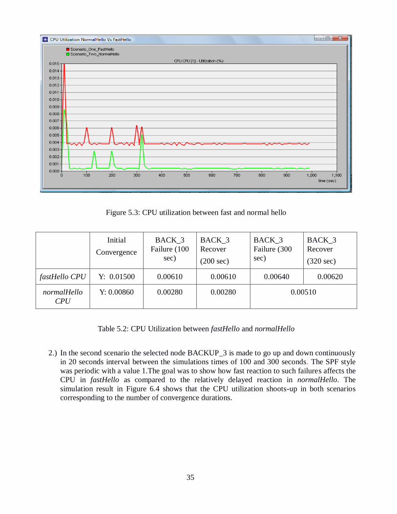
35

Figure 5.3: CPU utilization between fast and normal hello

Initial

Convergence

BACK_3

Failure (100

sec)

BACK_3

Recover

(200 sec)

BACK_3

Failure (300

sec)

BACK_3

Recover

(320 sec)

fastHello CPU Y: 0.01500 0.00610 0.00610 0.00640 0.00620

normalHello

CPU

Y: 0.00860 0.00280 0.00280 0.00510

Table 5.2: CPU Utilization between fastHello and normalHello

2.) In the second scenario the selected node BACKUP_3 is made to go up and down continuously

in 20 seconds interval between the simulations times of 100 and 300 seconds. The SPF style

was periodic with a value 1.The goal was to show how fast reaction to such failures affects the

CPU in fastHello as compared to the relatively delayed reaction in normalHello. The

simulation result in Figure 6.4 shows that the CPU utilization shoots-up in both scenarios

corresponding to the number of convergence durations.

36

Figure 5.4: fastHello vs. normalHello reaction to continuous flaps

3.) The third simulation in Figure 5.5 shows the effect of concurrent node failures and recoveries

on the CPU for fastHello. The effect was analyzed in three different scenarios. We used the

twelve nodes in the left side of the simulated topology in Figure 5.1 to create three different

scenarios. In the first scenario, the top four nodes were put down at a time at simulation time

100s and recovered at 200s. In the second scenario, a total of 8 nodes failed at simulation time

100s and recovered at time 200s. In the third scenario, all the 12 nodes were made to fail at

time 100s and recovered at 200s. The SPF style used was periodic one second to create the

maximum possible pressure on the CPU.

The 12 nodes, when seen in 3 pairs of each 4 nodes, have the same number of adjacencies to

the back bone nodes; BACK_1 for example. This creates an interesting scenario to observe the

CPU utilization trend on BACK_1 when different combinations of these pairs fail/recover at

different times.

37

Figure 5.5: CPU utilization for fastHello under concurrent failures

From this result, we were able to conclude the following.

The CPU utilization is highly dependent on the number of adjacencies that a router

has. As can be seen from the above figure, The CPU utilization is inversely

proportional with the number of failing nodes whereas it’s directly proportional with

the number of recovering nodes. This is of course is due to the fact that the more the

number of the adjacencies ,the more will be the corresponding number of LSAs that a

router needs to process, and OSPF operations including the SPF computation are

highly dependent on the size of the link state database that contains all these LSAs .

The Other interesting analysis is that even though the CPU consumption trend is

generally decreasing for the failure case and increasing for the recovery, the relative

changes are not the same i.e. it shows a sharp rise for the recovery and relatively a

small change for the failure. Well, it’s of course always easier to destroy than to create;

a lot of OSPF messages have to be exchanged and processed since the neighbor

relationships need to be re-created from scratch.

4.) The fourth part in Figure 5.6 shows how the network stability can be affected due to frequent

node failure/recovery when using different values for the SPF hold value. This can be shown

in OPNET Modeler using the next hop update parameter that shows the number of times the

next hop of a given route is updated. The selected node BACK_3 is made to flap 20 times in

10seconds interval between the simulation times 100 and 300 seconds. This time the

LSA_driven SPF style is used with initial delay of 1s and a hold value of 5s for the first

scenario and initial delay of 1s and a hold value of 15s for the second scenario.

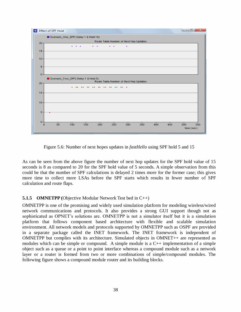
38

Figure 5.6: Number of next hopes updates in fastHello using SPF hold 5 and 15

As can be seen from the above figure the number of next hop updates for the SPF hold value of 15

seconds is 8 as compared to 20 for the SPF hold value of 5 seconds. A simple observation from this

could be that the number of SPF calculations is delayed 2 times more for the former case; this gives

more time to collect more LSAs before the SPF starts which results in fewer number of SPF

calculation and route flaps.

5.1.5 OMNETPP (Objective Modular Network Test bed in C++)

OMNETPP is one of the promising and widely used simulation platform for modeling wireless/wired

network communications and protocols. It also provides a strong GUI support though not as

sophisticated as OPNET’s solutions are. OMNETPP is not a simulator itself but it is a simulation

platform that follows component based architecture with flexible and scalable simulation

environment. All network models and protocols supported by OMNETPP such as OSPF are provided

in a separate package called the INET framework. The INET framework is independent of

OMNETPP but complies with its architecture. Simulated objects in OMNET++ are represented as

modules which can be simple or compound. A simple module is a C++ implementation of a simple

object such as a queue or a point to point interface whereas a compound module such as a network

layer or a router is formed from two or more combinations of simple/compound modules. The

following figure shows a compound module router and its building blocks.

39

Figure 5.7: OMNETPP simple/compound modules

A network model in OMNETPP is created using a special Network Description Language called the

NED language. All connections between simple/compound modules and other associated parameters

are described using the NED language.

5.1.5.1 OMNETPP simulation components

A simulation model in OMNETPP consists of the following files:

NED files: Like OTcl is for NS-2 or python/C++ is for NS-3, topology information in OMNETPP is

described using the NED language as mentioned above. The information contains the network name,

a detail description of the sub modules forming the network and the description of the connection

between them (channels, gates etc.).

Config. files: Contains OSPF configuration information; this includes information related to the areas

(area id, area address range etc.) and routers such as router id and the description of its interfaces.

Routing information: this includes the router IP addressing details, metric, multicast/broadcast

groups and static/default routing information.

Omnetpp.ini file: The Omnetpp.ini file describes what to run and with what parameters; it contains

the names of the NED file, the configuration file, the routing files, and other run-time parameters. The

following figure shows a screen dump of the above files in OMNET++ window.

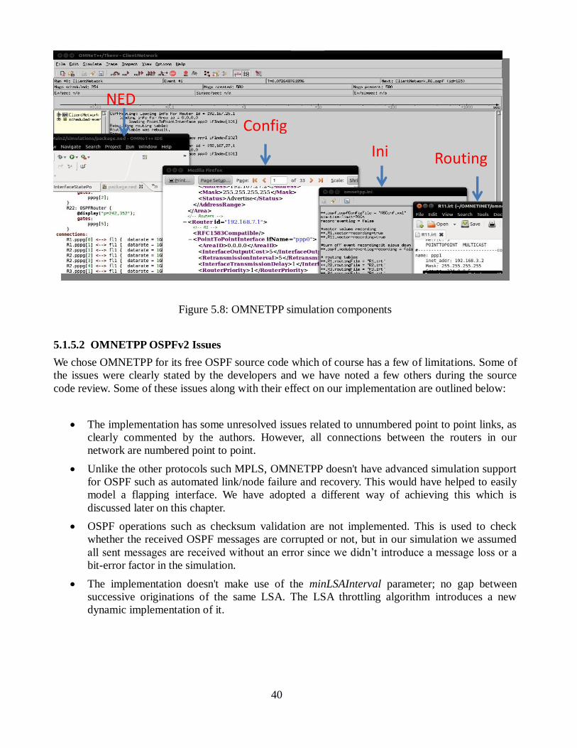
40

Figure 5.8: OMNETPP simulation components

5.1.5.2 OMNETPP OSPFv2 Issues

We chose OMNETPP for its free OSPF source code which of course has a few of limitations. Some of

the issues were clearly stated by the developers and we have noted a few others during the source

code review. Some of these issues along with their effect on our implementation are outlined below:

The implementation has some unresolved issues related to unnumbered point to point links, as

clearly commented by the authors. However, all connections between the routers in our

network are numbered point to point.

Unlike the other protocols such MPLS, OMNETPP doesn't have advanced simulation support

for OSPF such as automated link/node failure and recovery. This would have helped to easily

model a flapping interface. We have adopted a different way of achieving this which is

discussed later on this chapter.

OSPF operations such as checksum validation are not implemented. This is used to check

whether the received OSPF messages are corrupted or not, but in our simulation we assumed

all sent messages are received without an error since we didn’t introduce a message loss or a

bit-error factor in the simulation.

The implementation doesn't make use of the minLSAInterval parameter; no gap between

successive originations of the same LSA. The LSA throttling algorithm introduces a new

dynamic implementation of it.

NED file

Ini file

Routing file

Config file

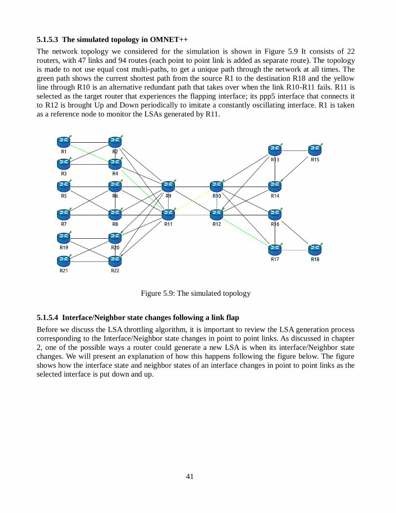
41

5.1.5.3 The simulated topology in OMNET++

The network topology we considered for the simulation is shown in Figure 5.9 It consists of 22

routers, with 47 links and 94 routes (each point to point link is added as separate route). The topology

is made to not use equal cost multi-paths, to get a unique path through the network at all times. The

green path shows the current shortest path from the source R1 to the destination R18 and the yellow

line through R10 is an alternative redundant path that takes over when the link R10-R11 fails. R11 is

selected as the target router that experiences the flapping interface; its ppp5 interface that connects it

to R12 is brought Up and Down periodically to imitate a constantly oscillating interface. R1 is taken

as a reference node to monitor the LSAs generated by R11.

Figure 5.9: The simulated topology

5.1.5.4 Interface/Neighbor state changes following a link flap

Before we discuss the LSA throttling algorithm, it is important to review the LSA generation process

corresponding to the Interface/Neighbor state changes in point to point links. As discussed in chapter

2, one of the possible ways a router could generate a new LSA is when its interface/Neighbor state

changes. We will present an explanation of how this happens following the figure below. The figure

shows how the interface state and neighbor states of an interface changes in point to point links as the

selected interface is put down and up.

42

Figure 5.10: Interface/Neighbor state changes

Normally, when an interface is brought down, the following sequence of actions are taken by the

router

The interface's state is changed to DOWN .This may necessitate a new LSA generation

(LSA1) that excludes the down link. The interface may not have a neighbor associated with it

in this case.

All the timers associated with the interface are cleared.

A kill neighbor’s signal(actually a function call to delete all the neighbor states associated

with that interface) is sent to all neighbor objects associated with the interface following

which all the neighbor data structures are cleared and also the inactivity timer(that fires every

routerDeadInterval amount) is cancelled. Finally the neighbor’s states are put to down. This is

followed by a new LSA generation (LSA2) that excludes the down link states.

When the interface is brought up again, its state immediately changes to Point-to-point(note that this

is not the case in broadcast links) and a new LSA (LSA3) is generated to advertise this, but the link is

advertised as a stub link if the adjacency over it is not yet fully established. The neighbor state

transitions all the way from init to full upon which the router once again generates an LSA declaring

the availability of a fully functional route (LSA5). The neighbor state may jump from an exchange

43

state to full state as shown in the figure following an exDone event if the link state request list of the

router is found empty(i .e all the LSAs are already exchanged). Note that if the second kill neighbor

signal is sent to a neighbor state that is in any of the states less than the full State, no LSA will be

generated as a result, rather the neighbor state is restarted from init.

The above sequences of actions were put ambiguously in OSPFv2 source code leading to unnecessary

LSA generation. That was corrected following the discussions with our supervisor. However, with the

LSA throttling feature enabled, we don’t have such issues as the LSA generation is no longer event

driven but rather controlled by the LSA throttling timers.

5.1.5.5 The convergence process in simulation

The simulation results of the CPU time taken for each of the convergence factors described in chapter

2 are shown in table 5.3 We will explain the approaches used below:

Failure detection time: This is the duration from the failure of a link/Node until the OSPF process is

informed of the failure. In our case, the failure detection time is the duration from the time the given

interface is brought down using the interfaceDown event triggered upon the expiry of the

interfaceDown timer until the router performs all the necessary changes following the failure (see

section 6.1.3.4) but before the corresponding LSA is originated.

Propagation time: this is the duration from the start of the LSA origination until it is received by the

farthest router in the network (depends on the network diameter). This includes the time for the LSA

origination, flooding, reception and processing time by a receiver which includes identifying the LSA

for new/duplicate, re-flooding and acknowledgment among others. An initial LSA delay time is also

added to this if any is configured.

SPF run time: this is the CPU time taken to compute SPT for the network. The SPT is computed for

the given network of 94 routes. Note that each point to point interface assumes a separate route in the

routing table and added to the routing table as a separate route unlike broadcast links where a single

route is added for adjacent links that share a common sub network address.

FIB Update time: OMNETPP simulation doesn't consider FIB update times; it assumes an ideal

router with FIB update time 0. So, routes are already added to the routing table when the SPF

computation returns. As a result, this time is considered zero in our case. Note that in real world

scenarios, the FIB update time takes the maximum share next to the event propagation time in the

convergence process. The table below shows the average CPU times for the above operations.

44

Operation Average CPU-time(ms) Remark

Failure Detection 0.050 Time from a failure of PPP6 interface of R11 until LSA

generation starts; this actually doesn’t correspond to the

real detection time as we manually down the interface

in the code itself.

Event propagation 145.96 Time from LSA generation by R11 (target Node) until

SPF starts at R1 (reference Node).LSA/SPF initial delay

is assumed 0.

SPF computation 2.65 SPF computation and routing table update

FIB update NA Not applicable

Total Convergence

Time

148.66 Total Convergence time for a down event

Table 5.3: Total convergence time

5.1.5.6 LSA Throttling

The LSA throttling algorithm works under the presence of a link flap. In the real case, the flap is

notified to the OSPF process by the available failure detection mechanism. Figure 5.11 shows the

periodic UP (U) and Down (D) Timers and the LSA throttling timers in action as the ppp5 interface of

R11 flaps.

Timers IntfDownTimer(D) IntfUPTimer(U) LSAInitialDelay(i) Hold(h) MaxDelay

Intervals(s) 2 3 1 2 32

Figure 5.11: LSA throttling timers

45

As can be seen from the figure, the interface down event (D) starts from time 20; the delay is to give

enough time for the initial convergence which is the total time that each router takes to acquire all the

routes in the network initially. The LSAInitialDelay(i) is assumed to be 1s; this is an important

parameter to be tuned carefully in real network deployments because it has a significant impact on the

convergence time. The general rule of thumb is to keep it as small as possible (5-10ms, Cisco) but

large enough to incorporate multiple changes that might occur synchronously (e.g. simultaneous link

failures when a routers fails). The hold value starts from 2s and it grows exponentially until

MaxDelay after which it keeps this value so long as the flap. It will be reset back to its initial value if

no sign of flap is detected for a duration of 2*MaxDelay. The Up and Down timers are rough

estimations fulfilling the following conditions:

The UP time (3s) is chosen in such a way that there would be enough time for Router11 to

establish a full neighbor relationship with its adjacent router R12 before it is brought down.

The Down time (2s) should give enough room for the adjacency to be fully torn down before

it is brought up again.

The inactivity timer is assumed not to fire following a down neighbor, for the down interval of

2 seconds is less than the routerDeadInterval which is 4 second and at least one hello must be

received before it expires. This is automatically taken care of by the OSPF process when the

neighbor state is brought down. But even if this timer fires leading to LSA generation, the

LSA generation is subjected to follow the LSA Throttling delay.

Below are shown the pseudo code for some parts of the implementations related to the timers.

Notations:

router is a pointer to a Router

intf is a pointer to an Interface nbr is a pointer to a Neighbor

msgHandler is a pointer to MessageHandler

Upon expiry(timer intfDownTimer) If router=TARGETROUTER then // get the target router with a flaping interface

Intf <--getInterfacebyId(intfId) // get a reference to an active interface

Set intf.state<--DOWN // fail the interface

Timer intfUPTimer<--router.getIntfUpTimer() // get a reference to the Up timer

start(timer intfUPTimer,double upInterval) // (re)schedule the UP timer

Upon expiry(timer intfUpTimer) intf<--intfUpTimer.getContextPointer() // get a reference to the interface from Set intf.state<--UP // the timer context and recover it

start(timer intfDownTimer,double downInterval) // reschedule the Down Timer

Upon expiry(timer stopTimer) // stop the flap timers and make sure the intf is Up finally

If isRunning(timer intfDownTimer) then

stopHandler.clearTimer(intfDownTimer)

else if isRunning(timer intfUPTimer) then

stopHandler.clearTimer(intfUpTimer)

If intf.getCurrentState()=DOWN then // make sure the interface is up finally

Set intf.CurrentState=UP

46

Upon expiry(timer lsaDelayTimer)

Intf<--lsaDelayTimer.getContextPointer() // get a reference to the interface from the timer context

// track the presence of a flap using the flap counters associated with each interface or using the neighbor

// inactivity/linkDown counter associated with the neighbors on each PPP interface // a sequence No. mismatch error may also occur leading to LSA generation when a router suddenly resets

// its sequence number due to interface Down event before the other peer detects the failure.

If intf.getFlapCounter()>=1 or

intf.getNeighbor.getInactivityCounter>=0 or

intf.getNeighbor.getLinkDownCounter>=0 or

intf.getNeighbor.seqNoMistmatchCounter>0 then

router.OriginateRouterLSA() // generate the LSA

If 2*intf.GetLSADelayInterval()>=MAXDELAY then // delay shouldn’t exceed MAXDELAY

intf.setLSADelayInterval(MAXDELAY)

Else intf.setLSADelayInterval(2*GetLSADelayInterval()) //double delay until MAXDELAY

msgHandler.startTimer(intf.lsaDelayTimer, intf.GetLSADelayInterval()) // re schedule delay timer // reset all the counters associated with a link/interface flap

reset(flapCounter)

reset(inactivityCounter)

reset(linkDownCounter)

reset(seqNoMMCounter)

Else intf.resetLSADelayInterval() // reset the delay interval to its initial if the flap stops

DelayHandler.clearTimer(router.lsaDelayTimer) // cancel the timer

Table 5.4: Pseudo codes for LSA Throttling timers

The following two figures show Router 11’s LSAs as they arrive at R1. Figure 5.12 shows LSA

arrivals without the LSA throttling feature and figure 5.13 shows the arrivals with LSA Throttling

enabled. The red spot at around simulation time 10 shows the initial convergence time; i.e. the last

route insertion time where R1 has installed all the 94 routes. This time is almost the same for all

routers with only a slight variation of a few milliseconds. The average value is 10.092 simulation

seconds.

Figure 5.12: Original LSAs as they arrive on R1

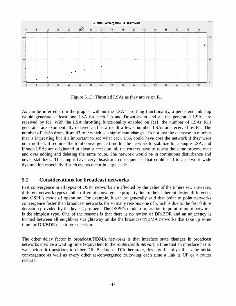
47

Figure 5.13: Throttled LSAs as they arrive on R1

As can be inferred from the graphs, without the LSA Throttling functionality, a persistent link flap

would generate at least one LSA for each Up and Down event and all the generated LSAs are

received by R1. With the LSA throttling functionality enabled on R11, the number of LSAs R11

generates are exponentially delayed and as a result a fewer number LSAs are received by R1. The

number of LSAs drops from 43 to 9 which is a significant change. It’s not just the decrease in number

that is interesting but it’s important to see what each LSA could have cost the network if they were

not throttled. It requires the total convergence time for the network to stabilize for a single LSA, and

if such LSAs are originated in close succession, all the routers have to repeat the same process over

and over adding and deleting the same route. The network would be in continuous disturbance and

never stabilizes. This might have very disastrous consequences that could lead to a network wide

dysfunction especially if such events occur in large scale.

5.2 Considerations for broadcast networks

Fast convergence in all types of OSPF networks are affected by the value of the timers set. However,

different network types exhibit different convergence property due to their inherent design differences

and OSPF’s mode of operation. For example, it can be generally said that point to point networks

convergence faster than broadcast networks for so many reasons one of which is due to the fast failure

detection provided by the layer 2 protocol. The OSPF’s mode of operation in point to point networks

is the simplest type. One of the reasons is that there is no notion of DR/BDR and an adjacency is

formed between all neighbors straightaway unlike the broadcast/NBMA networks that take up some

time for DR/BDR election/re-election.

The other delay factor in broadcast/NBMA networks is that interface state changes in broadcast

networks involve a waiting time (equivalent to the routerDeadInterval), a time that an interface has to

wait before it transitions to either DR, Backup or DRother state, this significantly affects the initial

convergence as well as every other re-convergence following each time a link is UP or a router

restarts.

48

While the presence of DR/BDR in broadcast networks reduces the number of adjacencies, it exposes

the network to a single point of failure and also it requires the DR/BDR to originate a new type 2

LSAs to communicate changes to all the nodes in the network. This increases the overhead in the

network. If both the DR and BDR happen to fail at a time, the network performance will be highly

degraded. Multiple adjacencies are dropped simultaneously and a new DR/BDR re-election needs to

be undergone. All topology changes in the meantime will not be communicated leading to a delayed

convergence.

The LSA generation delay algorithm applies to all types of OSPF networks in the presence of a link

flap, but the effect varies a little. This is due to the difference in the traditional failure detection

mechanisms used in those network types. Unlike the point to point networks that have link layer

failure detection mechanism, broadcast networks can’t detect failures that occur behind the switch so

quickly but after the routerDeadInterval. This means that they are unresponsive to frequent link flaps

that may happen within the routerDeadInterval in contrast to the former that are aware of such events

as they occur and react instantly. The use of a BFD session over a layer 2 switch is an alternative fast

failure detection mechanism for broadcast links.

49

6. Conclusion and Future work

OSPF is one of the prominent and widely studied IGP routing protocols in ISPs and enterprise

networks. Since the latest RFC2328 released more than a decade ago, there have been numerous

changes in both its traditional configuration of parameter such as timer values as well as changes due

to optimized ways of working in many of its operations. Most of the important operations of OSPF

that contribute to its fast convergence such as failure detection, SPF calculation, LSA generation and

flooding are controlled by timers. Some of these timers have traditionally been considered as

architectural constants whereas as the rest were a one-time set fixed values. Modern experiences and

research works suggest a dynamic implementation of these timers for a safer network operation and

faster convergence to failures. Dynamic timers are generally set to a small initial value based on the

expected network stability level and the values vary with the experienced network load. This adds

robustness for the OSPF operation at times of instabilities as well as improves the network

convergence speed at times of stable network operations.

This work in part revises what has been achieved in OSPF fast convergence so far, with a more focus

on the use of dynamic timers. Stability issues that come with reducing the timer values have also been

discussed supported by simulation results for some selected scenarios. The simulation results show

that while fast hellos of one second are good choices for fast neighbor discovery and failure detection,

they may not be that effective for continuous but brief link/router breakdowns that are common on

real network deployments. We have also concluded that the CPU consumption highly depends on the

number of adjacencies a router has. This work has also introduced the pseudo code as well as the

implementation and evaluation of the LSA throttling algorithm. The simulation results demonstrate

that an OSPF network using this feature has a much lower number of LSAs generated at times of

persistent link/node flaps. Having this dynamic technique is crucial to achieve fast convergence

taking the CPU and network stability into consideration.

Fast convergence to network changes is one of the desirable properties of OSPF and other routing

protocols. Experiences indicate a combination of different techniques are used in each operational

phases of OSPF to achieve sub-second convergence. Simulation results modeling real ISP networks

of hundreds of nodes show that the hello timers can safely be reduced to a few hundreds of

milliseconds for fast failure detection. Although the use of fast IGP keep alive timers seems to be

inefficient in terms of the heavy processing load, a dynamic implementation of this, along with a

routing protocol independent BFD technique is still highly recommended for fast failure detection on

broadcast networks. BFD with IP-event dampening technique is a recommended combination for fast

failure detection as well as suppression of false alarms. LSA throttling is used to provide dynamically

controlled LSA generation against link flaps. SPF Throttling is best used with LSA throttling to

provide dynamically controlled SPF computations for self-generated or flooded LSAs. While using

these throttling techniques, it is very important to tune the initial delays carefully as it highly impacts

the convergence duration for occasional and transient network failures.

New variants of SPF algorithm such as iSPF with a dynamic scheduling scheme are best to minimize

the CPU overhead on large networks. Dynamically tuned packet pacing delay timers are also

recommended for optimized flooding and retransmission. Incremental FIB update techniques provide

optimized performance by only updating modified IP route prefixes instead of a full dump.

50

Recent proposals on minimizing packet drops during the convergence period suggest a mechanism to

avoid communication breakdown at times of link/node failures through the use of alternate locally

determined paths without requiring explicit notification of the failures globally. Details can be found

on as RFC 5714, 2010.

Future works on OSPF fast convergence and stability issues may consider the implementation of the

LSA throttling algorithm or other similar dynamic timer techniques on broadcast networks. We also

would like to recommend the use of emulators instead of simulators for a close-to-real network

analysis of results as the emulated network can be extended to a real network node.

51

References

[1]. Moy John T, ‘OSPF version 2’, Internet Engineering Task Force, Request For Comments,

2328, April 1998.

[2]. ‘OSPF Support for Fast Hellos’, Cisco, March 2012.

[3]. IXIA, ‘Open Shortest Path First (OSPF) Conformance and Performance Testing Sample Test

Plans’, March 2012, IXIA.

[4]. Moy John T, ‘OSPF Network Design Solutions, Second Edition ‘, Cisco Systems, Inc, 2003.

[5] Moy John T, ‘OSPF: Anatomy of an Internet Routing Protocol’, Addison-Wesley Professional,

February 1998.’

[6] Jing Fu1, Peter Sjödin, and Gunnar Karlsson, ‘Towards Distributed Router Architectures and

Centralized Control Architectures in IP Networks’, School of Information and Communication

Technology KTH, Royal Institute of Technology, SE-100 44, Stockholm, Sweden.

[7] Goyal M, Soperi M, Bacce lli E, Choudhury G, Shaikh A, Hosseini H, and Trivedi K,

‘Improving Convergence Speed and Scalability in OSPF: A Survey ‘, IEEE Communications

Surveys & Tutorials ,Accepted For Publication , 11 December 2010.

[8] Fang W, Shanzhi C, Xin L, Yuhong L, ‘A Route Flap Suppression Mechanism Based on

Dynamic Timers in OSPF Network’, The 9th International Conference for Young Computer

Scientists, IEEE,2008.

[9] Anindya B and Riecke Jon G,’ Stability Issues in OSPF Routing ‘, SIGCOMM’01, August 27-

31, 2001.

[10] ‘Bidirectional Forwarding Detection for OSPF’, Cisco, 2005.

[11] Katz D and Ward D, ‘Bidirectional Forwarding Detection (BFD)’ , Internet Engineering Task

Force(IETF), RFC 5880, Juniper Networks , June 2010.

[12] ‘OSPF Link-State Advertisement Throttling’, Cisco Systems, Inc, First Published: April 15,

2003 October and Last Updated: February 26, 2010.

[13] Pierre F, Clarence F, John E, Olivier B, ’Achieving sub-second IGP convergence in large IP

networks ‘, IEEE, 2009.

[14] Aman S, Albert G, ‘Experience in Black-box OSPF Measurement’,

SIGCOMM’01, November 01 - 02, 2001.

52

[15] Cengiz A, Van J, Haobo Y, ‘Towards Millisecond IGP Convergence’, Internet Draft, Packet

Design, November 2000.

[16] Abdelali A, Mohamed E, Driss El O, ‘Fast Convergence Mechanisms and Features

Deployment within Operator Backbone Infrastructures’, IEEE, 2009.

[17] Goyal M, Soperi M, Hosseini H, Trivedi KS, ‘Analyzing the Hold Time Schemes to Limit the

Routing Table Calculations in OSPF Protocol’, International Conference on Advanced

Information Networking and Applications, IEEE, 2009.

[18] Gagan L, Choudhury, ‘Prioritized Treatment of Specific OSPF Version 2

Packets and Congestion Avoidance’, Request For Comment 4222 , AT&T, October, 2004.

[19] ‘OSPF LSA Group Pacing’, Cisco IOS Software Releases 11.3, Cisco, April 2012.

[20] ‘OSPF Update Packet-Pacing Configurable Timers’, Cisco, Cisco IOS Release 12.2(14) S,

November 8, 2012

[21] ‘IP Event dampening’, Cisco, Cisco IOS Software Releases 12.0 S, September 10, 2010.

[22] Doyle J, Matthew C Kolon, ‘The complete Reference, Juniper Network Routers’, McGraw-

Hill Osborne Media, 2002.

[23] DIJKSTRA E.W, ‘A Note on Two Problems in Connection with Graphs’, Numer. Math 1:269-

71, Mathematisch Centrum, Amsterdam, The Netherlands,1959.

[24] Xuezhi J, Mingwei X, Qi L, ‘DHOSPF: Adaptive Parallel Routing Table Computation for

Next Generation Routers’, International Journal of Digital Content Technology and its

Applications. Volume 5, Number 7, July 2011.

[25] ‘OSPF Shortest Path First Throttling’, Cisco, April 2012.

[26] Coltun R, Ferguson D, Lindem A, Ed. ‘OSPF for IPv6’, Network Working Group, RFC:

5340, July 2008.

[27] Goyal M, Xie W, Soperi M, Hosseini SH, Vairavan K, ‘Scheduling Routing Table Calculations

to Achieve Fast Convergence in OSPF Protocol’, Internet Draft November 29, 2006.

[28] Moy J, Pillay-Esnault P, Lindem A, ‘Graceful OSPF Restart’, Network Working Group, RFC:

3623, November 2003.

[29] Yaoqing L, Xin Z, Kyuhan N, Lan W, Beichuan Z, ‘Incremental Forwarding Table

Aggregation’ , December 2010.

[30] Mukul G, Ramakrishnan K. K. and Wu-chi F ,’Achieving Faster Failure Detection in OSPF

Networks’, in Proc. IEEE International Conference on Communications (ICC 2003), 2003.

[31] Pillay-Esnault P, ‘OSPF refresh and flooding reduction in stable topologies’, RFC 4136, IETF

, July 2005.

53

[32] Samad Sumi A, Shenoy S.K., Santhosh Kumar G, Pillai P.R.S, ‘A Survey of Modeling and

Simulation Tools for Underwater Acoustic Sensor Networks’, International Journal of

Research and Reviews in Computer Science (IJRRCS), SI: Simulation, Benchmarking and

Modeling of Systems and Communication Networks, April, 2011.

[33] Jianli P, Prof. Raj J, ‘A Survey of Network Simulation Tools: Current Status and Future

developments’, November 24, 2008.

[34] ‘IP Connectivity and Routing’, Technical Product Description, Ericsson, viewed November

2012.

[35] Mohd Soperi B, Mohd Z,’ Dissertation-Soperi’, April 2012.

[36] Amir S, Biswajit N, ‘Improving Network Convergence Time and Network Stability of an

OSPF-Routed IP Network’, 2005.

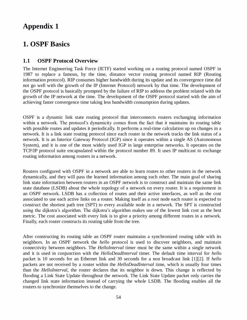
54

Appendix 1

1. OSPF Basics

1.1 OSPF Protocol Overview

The Internet Engineering Task Force (IETF) started working on a routing protocol named OSPF in

1987 to replace a famous, by the time, distance vector routing protocol named RIP (Routing

information protocol). RIP consumes higher bandwidth during its update and its convergence time did

not go well with the growth of the IP (Internet Protocol) network by that time. The development of

the OSPF protocol is basically prompted by the failure of RIP to address the problem related with the

growth of the IP network at the time. The development of the OSPF protocol started with the aim of

achieving faster convergence time taking less bandwidth consumption during updates.

OSPF is a dynamic link state routing protocol that interconnects routers exchanging information

within a network. The protocol’s dynamicity comes from the fact that it maintains its routing table

with possible routes and updates it periodically. It performs a real-time calculation up on changes in a

network. It is a link state routing protocol since each router in the network tracks the link status of a

network. It is an Interior Gateway Protocol (IGP) since it operates within a single AS (Autonomous

System), and it is one of the most widely used IGP in large enterprise networks. It operates on the

TCP/IP protocol suite encapsulated within the protocol number 89. It uses IP multicast to exchange

routing information among routers in a network.

Routers configured with OSPF in a network are able to learn routes to other routers in the network

dynamically, and they will pass the learned information among each other. The main goal of sharing

link state information between routers in an OSPF network is to construct and maintain the same link

state database (LSDB) about the whole topology of a network on every router. It is a requirement in

an OSPF network. LSDB has a collection of routes and their active interfaces, as well as the cost

associated to use each active links on a router. Making itself as a root node each router is expected to

construct the shortest path tree (SPT) to every available node in a network. The SPT is constructed

using the dijkstra’s algorithm. The dijkstra’s algorithm makes use of the lowest link cost as the best

metric. The cost associated with every link is to give a priority among different routes in a network.

Finally, each router constructs its routing table from the tree.

After constructing its routing table an OSPF router maintains a synchronized routing table with its

neighbors. In an OSPF network the hello protocol is used to discover neighbors, and maintain

connectivity between neighbors. The HelloInterval timer must be the same within a single network

and it is used in conjunction with the HelloDeadInterval timer. The default time interval for hello

packet is 10 seconds for an Ethernet link and 30 seconds for a non broadcast link [1][2]. If hello

packets are not received by a router within the HelloDeadInterval time, which is usually four times

than the HelloInterval, the router declares that its neighbor is down. This change is reflected by

flooding a Link State Update throughout the network. The Link State Update packet only carries the

changed link state information instead of carrying the whole LSDB. The flooding enables all the

routers to synchronize themselves to the change.

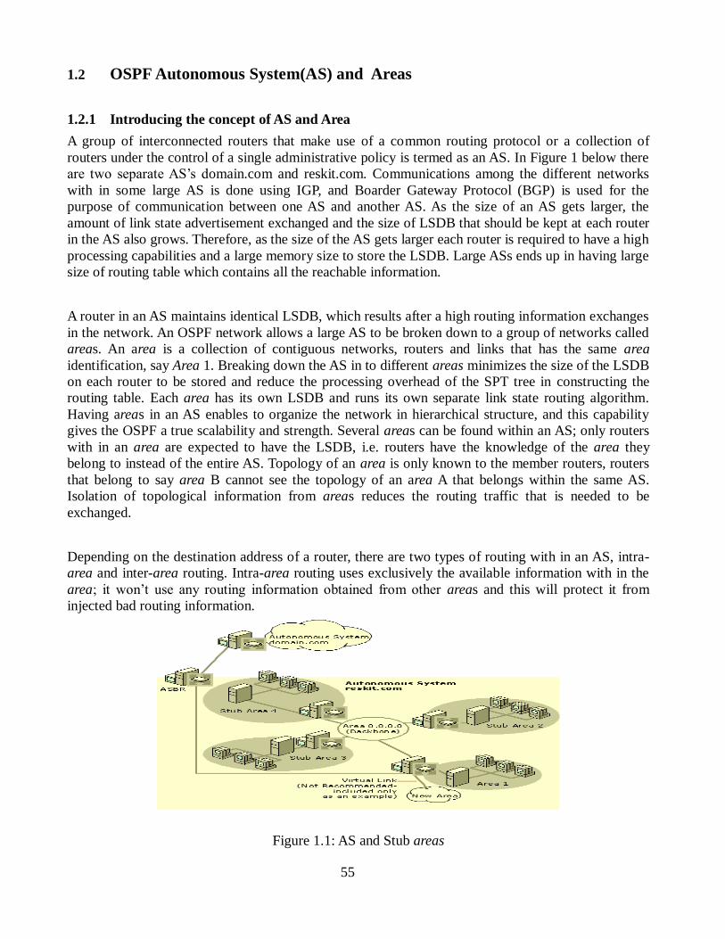
55

1.2 OSPF Autonomous System(AS) and Areas

1.2.1 Introducing the concept of AS and Area

A group of interconnected routers that make use of a common routing protocol or a collection of

routers under the control of a single administrative policy is termed as an AS. In Figure 1 below there

are two separate AS’s domain.com and reskit.com. Communications among the different networks

with in some large AS is done using IGP, and Boarder Gateway Protocol (BGP) is used for the

purpose of communication between one AS and another AS. As the size of an AS gets larger, the

amount of link state advertisement exchanged and the size of LSDB that should be kept at each router

in the AS also grows. Therefore, as the size of the AS gets larger each router is required to have a high

processing capabilities and a large memory size to store the LSDB. Large ASs ends up in having large

size of routing table which contains all the reachable information.

A router in an AS maintains identical LSDB, which results after a high routing information exchanges

in the network. An OSPF network allows a large AS to be broken down to a group of networks called

areas. An area is a collection of contiguous networks, routers and links that has the same area

identification, say Area 1. Breaking down the AS in to different areas minimizes the size of the LSDB

on each router to be stored and reduce the processing overhead of the SPT tree in constructing the

routing table. Each area has its own LSDB and runs its own separate link state routing algorithm.

Having areas in an AS enables to organize the network in hierarchical structure, and this capability

gives the OSPF a true scalability and strength. Several areas can be found within an AS; only routers

with in an area are expected to have the LSDB, i.e. routers have the knowledge of the area they

belong to instead of the entire AS. Topology of an area is only known to the member routers, routers

that belong to say area B cannot see the topology of an area A that belongs within the same AS.

Isolation of topological information from areas reduces the routing traffic that is needed to be

exchanged.

Depending on the destination address of a router, there are two types of routing with in an AS, intra-

area and inter-area routing. Intra-area routing uses exclusively the available information with in the

area; it won’t use any routing information obtained from other areas and this will protect it from

injected bad routing information.

Figure 1.1: AS and Stub areas

56

1.2.2 OSPF Area Types

1.2.2.1 Backbone Areas

The backbone area is the first and special area that should be built when an OSPF network is

configured. It is denoted by area 0 and can be described as 0.0.0.0[1]. Once a backbone area is

configured other areas connect to it. Inter-area communication is done using the backbone as a hub

.The backbone area includes routers that are located on boarder of areas called Area Boarder Routers

(ABRs). Routers that are found in the backbone need to be adjacent but if they are not physically

adjacent then virtual links can be configured for their connection [1]. A traffic flow between two non-

backbone areas area 1 and area 3 in the Figure1 above, is done in a way that the traffic first flows

from area 1 to the backbone area then the traffic flows through the backbone area 0.0.0.0, and finally

the traffic is directed to the final destination area 3.

1.2.2.2 Stub Area

Stub areas in OSPF network are areas with a single exit point, designed usually for routers with

limited resource capabilities like memory [3]. The stub area is only connected to the backbone area

and it works in a way that no outside traffic from the AS can be flooded to it. This allows routers in

the stub area to maintain a small link state database. Stub areas however accept route information

about other areas within the same domain (inter-area routing information). An ABR that is

configured for a stub network injects a default route, instead of advertising external routes, into the

stub area so that the routers inside the stub can use it to reach out to external networks. Stub areas

can be configured for a sub or branch offices that may not require knowing route to other sub branch

offices instead it will use the default route to reach the main office and from there it can find all route

information.

1.2.2.3 Totally Stubby Areas

As stub area, a totally stubby area is only connected to the backbone area and does not allow external

routes to be flooded to it. It only allows intra-area and the default routes to be propagated within the

area, which means routers only keep routing information about the totally stubby area and the default

route in their LSDB. All inside routers use the default route injected by the ABR ,configured at the

stubby area, in order to route any traffic between the totally stubby area and other areas within the

same AS or external to the AS.

1.2.2.4 Not So Stubby Areas (NSSA)

Figure 1.2: NSSA

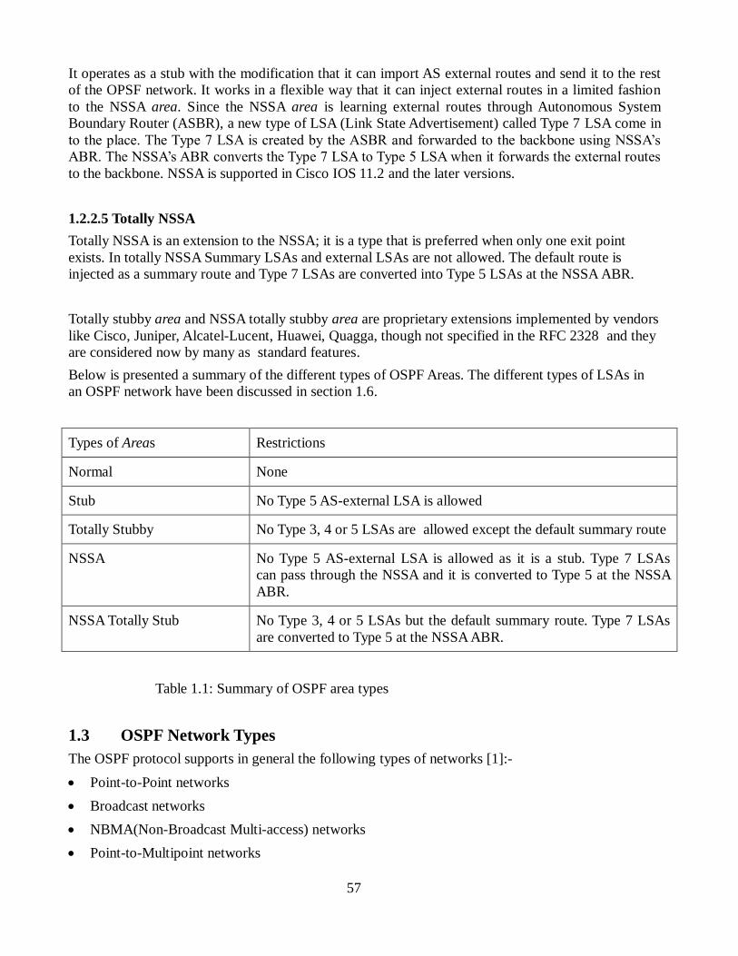
57

It operates as a stub with the modification that it can import AS external routes and send it to the rest

of the OPSF network. It works in a flexible way that it can inject external routes in a limited fashion

to the NSSA area. Since the NSSA area is learning external routes through Autonomous System

Boundary Router (ASBR), a new type of LSA (Link State Advertisement) called Type 7 LSA come in

to the place. The Type 7 LSA is created by the ASBR and forwarded to the backbone using NSSA’s

ABR. The NSSA’s ABR converts the Type 7 LSA to Type 5 LSA when it forwards the external routes

to the backbone. NSSA is supported in Cisco IOS 11.2 and the later versions.

1.2.2.5 Totally NSSA

Totally NSSA is an extension to the NSSA; it is a type that is preferred when only one exit point

exists. In totally NSSA Summary LSAs and external LSAs are not allowed. The default route is

injected as a summary route and Type 7 LSAs are converted into Type 5 LSAs at the NSSA ABR.

Totally stubby area and NSSA totally stubby area are proprietary extensions implemented by vendors

like Cisco, Juniper, Alcatel-Lucent, Huawei, Quagga, though not specified in the RFC 2328 and they

are considered now by many as standard features.

Below is presented a summary of the different types of OSPF Areas. The different types of LSAs in

an OSPF network have been discussed in section 1.6.

Types of Areas Restrictions

Normal None

Stub No Type 5 AS-external LSA is allowed

Totally Stubby No Type 3, 4 or 5 LSAs are allowed except the default summary route

NSSA No Type 5 AS-external LSA is allowed as it is a stub. Type 7 LSAs

can pass through the NSSA and it is converted to Type 5 at the NSSA

ABR.

NSSA Totally Stub No Type 3, 4 or 5 LSAs but the default summary route. Type 7 LSAs

are converted to Type 5 at the NSSA ABR.

Table 1.1: Summary of OSPF area types

1.3 OSPF Network Types

The OSPF protocol supports in general the following types of networks [1]:-

Point-to-Point networks

Broadcast networks

NBMA(Non-Broadcast Multi-access) networks

Point-to-Multipoint networks

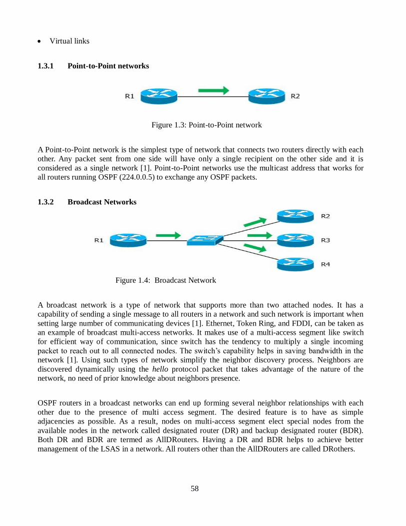
58

Virtual links

1.3.1 Point-to-Point networks

Figure 1.3: Point-to-Point network

A Point-to-Point network is the simplest type of network that connects two routers directly with each

other. Any packet sent from one side will have only a single recipient on the other side and it is

considered as a single network [1]. Point-to-Point networks use the multicast address that works for

all routers running OSPF (224.0.0.5) to exchange any OSPF packets.

1.3.2 Broadcast Networks

Figure 1.4: Broadcast Network

A broadcast network is a type of network that supports more than two attached nodes. It has a

capability of sending a single message to all routers in a network and such network is important when

setting large number of communicating devices [1]. Ethernet, Token Ring, and FDDI, can be taken as

an example of broadcast multi-access networks. It makes use of a multi-access segment like switch

for efficient way of communication, since switch has the tendency to multiply a single incoming

packet to reach out to all connected nodes. The switch’s capability helps in saving bandwidth in the

network [1]. Using such types of network simplify the neighbor discovery process. Neighbors are

discovered dynamically using the hello protocol packet that takes advantage of the nature of the

network, no need of prior knowledge about neighbors presence.

OSPF routers in a broadcast networks can end up forming several neighbor relationships with each

other due to the presence of multi access segment. The desired feature is to have as simple

adjacencies as possible. As a result, nodes on multi-access segment elect special nodes from the

available nodes in the network called designated router (DR) and backup designated router (BDR).

Both DR and BDR are termed as AllDRouters. Having a DR and BDR helps to achieve better

management of the LSAS in a network. All routers other than the AllDRouters are called DRothers.

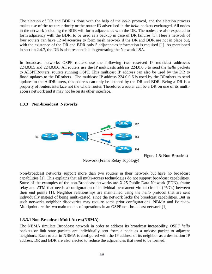
59

The election of DR and BDR is done with the help of the hello protocol, and the election process

makes use of the routers priority or the router ID advertised in the hello packets exchanged. All nodes

in the network including the BDR will form adjacencies with the DR. The nodes are also expected to

form adjacency with the BDR, to be used as a backup in case of DR failures [1]. Here a network of

four routers can have 12 adjacencies to form mesh network if the DR and BDR are not in place but,

with the existence of the DR and BDR only 5 adjacencies information is required [1]. As mentioned

in section 2.4.7, the DR is also responsible in generating the Network LSA.

In broadcast networks OSPF routers use the following two reserved IP multicast addresses

224.0.0.5 and 224.0.0.6. All routers use the IP multicasts address 224.0.0.5 to send the hello packets

to AllSPFRouters, routers running OSPF. This multicast IP address can also be used by the DR to

flood updates to the DRothers. The multicast IP address 224.0.0.6 is used by the DRothers to send

updates to the AllDRouters, this address can only be listened by the DR and BDR. Being a DR is a

property of routers interface not the whole router. Therefore, a router can be a DR on one of its multi-

access network and it may not be on its other interface.

1.3.3 Non-broadcast Networks

Figure 1.5: Non-Broadcast

Network (Frame Relay Topology)

Non-broadcast networks support more than two routers in their network but have no broadcast

capabilities [1]. This explains that all multi-access technologies do not support broadcast capabilities.

Some of the examples of the non-Broadcast networks are X.25 Public Data Network (PDN), frame

relay and ATM that needs a configuration of individual permanent virtual circuits (PVCs) between

their end points [1]. Neighbor relationships are maintained using the hello protocol that are sent

individually instead of being multi-casted, since the network lacks the broadcast capabilities. But in

such networks neighbor discoveries may require some prior configurations. NBMA and Point-to-

Multipoint are the two main modes of operations in an OSPF non-broadcast network [1].

1.3.3.1 Non-Broadcast Multi-Access(NBMA)

The NBMA simulate Broadcast network in order to address its broadcast incapability. OSPF hello

packets or link state packets are individually sent from a node as a unicast packet to adjacent

neighbors. Each router in NBMA is configured with the IP address of its neighbor as a destination IP

address. DR and BDR are also elected to reduce the adjacencies that need to be formed.

60

1.3.3.2 Point-to-Multipoint

As its name describes the Point-to-Multipoint treat the non-broadcast network as a collection of

Point-to-Point links and does not try to emulate the broadcast capability. As in NBMA individual

hello packets replication is needed but in this approach there is no need for DR or BDR that is no

Type-2 LSA.

1.3.4 Virtual links

A Virtual link is a link that is used to connect to the backbone through a non-backbone area. In such

links OSPF packets are sent as unicast.

1.4 OSPF Router Types

1.4.1 Backbone routers

Back bone routers are routers that belong to the backbone area (area 0). These routers can have one

or more interfaces in the backbone area. The area 0 is expected to have at least one backbone router

in its area [1].

1.4.2 Internal routers

Internal routers are those that have all their interfaces inside one area only, they are connected only to

one area [1].

1.4.3 Area Border Routers( ABRs)

ABRs are routers that are connected to more than one area. They are usually placed at the boarder of

an area to connect a non-backbone area to the backbone one, having its interfaces to both areas.

ABRs have multiple LSDBs, one for each attached area.

1.4.4 Autonomous System Border Routers(ASBRs)

ASBRs are routers that connect one AS to another AS that runs under different protocol. ASBRs are

routers that are used to distribute external routes from outside the AS.

1.5 OSPF Packet Types

Packet name Type Description

Hello 1 To discover and maintain neighbors

Database description 2 Summarize database contents

LinkState Request 3 A request to obtain LSAs from neighbor routers,

sent during the state of exchange, Loading, or Full.

LinkState Update 4 Used at the time of flooding, to send update to

neighbor routers.

LinkState acknowledgement 5 Acknowledgement that an LSA has been received.

Table 1.2: OSPF Packet Types

61

1.6 OSPF LSA Types

In an OSPF networks routers usually have different types of LSAs that are exchanged to describe the

link states associated with a router. The main types of LSAs in an OSPFv2 protocol are described

below.

1.6.1 Router LSA( Type-1 LSA)

Router LSA is usually characterized as Type 1 LSA [1].It is an LSA that describes the router’s

interface status and the cost associated with each link. Its flooding scope is only limited to the area it

belongs to. While generating the router LSAs, the originators router’s ID is used as the link state ID

that identifies the source. Router LSA includes the entire interface that the router has with in the area

in one single LSA packet [8].

1.6.2 Network LSA ( Type-2 LSA)

Network LSA is usually termed as Type 2 LSA, generated by the DR routers on behalf of the subnet

[1]. It is generated both in broadcast and NBMA networks, and it describes all the available routers

including the DR within an area. Network LSAs are flooded only with in the area they belong to, and

they use the DR’s IP interface address as a link state ID to identify the source.

1.6.3 Summary LSA ( Type-3 and Type-4 LSA)

An ABR, connected to more than one area, has the capability of summarizing all the routes that it has

learned from one area and passes it to other areas it is connected to, inter-area communications [1].

Several routes information is summarized in to a single prefix to create summary LSAs. This reduces

the size of the routing table or the information that should exist in link-state advertisements and

LSDB. The characterization of summary LSA generated by ABRs is based on the type of the

destination. If the destination is an ASBR the summary LSA generated is Type 4 summary LSA and

the ASBR’s router ID is used as a link state ID otherwise it is Type-3 LSA and the destination ABR’s

ID is used as the link state ID of the LSA [1].

1.6.4 AS External LSA ( Type-5 LSA)

Route information external to the AS are originated by the ASBRs and are characterized as type 5

LSAs [1].

1.6.5 Type-7 LSA

An ASBR in NSSA flexibly accepts external route information that is characterized as Type-7 LSA

and it can travel through the NSSA. The Type-7 LSA is then converted to Type-5 LSA by the NSSA’s

ABR to the backbone, as the LSA is routed to the rest of the network. The following table

summarizes the different types of LSAs in an OSPF network.

62

Name of the LSAs Type Created due to

Router LSA 1 Changes in the link status(up/down),

Changes in the link cost/bandwidth

Neighboring routers changes to/from the FULL state

The changes in the state of one of the router's that is

configured as virtual links

Network LSA 2 Changes in the Network's DR

If router itself is a DR and one of the neighboring routers

changes to/from the FULL state.

Summary LSA ¾ An intra-area or inter-area route has been

added/deleted/modified in the routing table.

Newly attached router to an area

AS-external-LSA 5 A router is no longer an ASBR.

An external route gained through direct experience with an

external routing protocol (like BGP) changes.

Table 1.3: LSA Types [1]

1.7 Basic operation of OSPF

Basic step by step operations are involved in the OSPF network which finally results in a converged

network. The steps involved are discovering neighbors, synchronizing link state database, doing route

calculations and finally populating the routing table with the optimal route information.

1.7.1 Neighbor discovery

In OSPF network routers that are adjacent with each other form a neighbor relationship, in order to

exchange routing information and maintain that relationship after the formation of the adjacency [1].

Such adjacency formation requires directly connected routers, and the interfaces used to be within the

same area.

In an OSPF network the hello protocol is used to dynamically discover neighbors and keep an eye on

them once a neighbor relationship is formed. The hello protocol also helps to elect the DR and BDR

to which each OSPF router should make adjacency with [1].While trying to establish fully adjacent

neighbor relationships, OSPF neighbor routers goes through different states: Down, Attempt, Init, and

2-Way, Ex-start, Exchange, Loading, and Full.

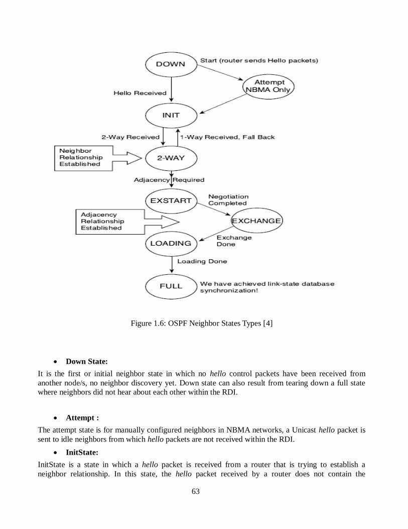
63

Figure 1.6: OSPF Neighbor States Types [4]

Down State:

It is the first or initial neighbor state in which no hello control packets have been received from

another node/s, no neighbor discovery yet. Down state can also result from tearing down a full state

where neighbors did not hear about each other within the RDI.

Attempt :

The attempt state is for manually configured neighbors in NBMA networks, a Unicast hello packet is

sent to idle neighbors from which hello packets are not received within the RDI.

InitState:

InitState is a state in which a hello packet is received from a router that is trying to establish a

neighbor relationship. In this state, the hello packet received by a router does not contain the

64

receiver’s router ID .The receiver node is expected to include the sender’s ID in its hello packet as an

acknowledgement that a valid hello packet has been received by it.

2-Way state:

It is a state that follows the InitState in which a bi-directional communication is established between

two routers. This state is achieved when the receiving node finds its own router ID inside the hello

packet sent by another node; both routers have seen each other’s hello packets at this stage and they

are considered as neighbors. DR and BDR are elected for broadcast and non-broadcast networks. A

router becomes full state only with the DR and BDR and stays in a 2-Way state with all other

neighbors. But, on a point-to-point or point-to-multipoint networks a router becomes in full state with

all connected routers in the network.

1.7.2 Database synchronizations

Exchange start (Ex-start) state:

Once the DR and BDR are elected in the 2-way state, routers start to exchange link state information

with their DR and BDR which transit it to Exstart [3]. In this state router establish a Master-Slave

relationship on a neighbor basis and chooses the initial sequence number used for the DBD packets to

be exchanged among them [3]. A router is elected as Master on the basics of its router ID.

Exchange state:

The Ex-start transits to the Exchange state once the Master-Slave and sequence number is negotiated

between adjacent neighbors. In this state, neighbors exchange database description packet that

describes their database [8]. The database description packet contains only the LSA header that

describes the content of their LSDB. The database description packet sequence number is

incremented only by the Master and it has to be acknowledged by the slave in explicit manner [8]. In

the process of Exchange state, routers can also send and receive link-state request and update that

contains the entire LSA .After database information has been exchanged among neighbors, the

Exchange state can change to Loading or Full state.

Loading state:

Loading state is when the Link state request list is not empty. Based on the information provided in

the database description packets, routers make a request for link state information they don’t have

.The requested router responds with a Link State Update packet that contains the information being

requested and this update is also acknowledged by the receiver. When the exchange process is

completed between neighboring routers their state transfers to the Full state.

Full state:

It is considered as the fully functional state of OSPF neighbors where the Link state request list is

empty and neighbors are fully adjacent with each other. The following figure illustrates the different

types of OSPF message exchanges from adjacency start-up to completion.

65

Figure 1.7: an adjacency bring-up example [1]

1.7.3 Route calculations

Once link state information is synchronized among routers, each router in a network performs a route

calculation. The route calculation is based on the SPF (Shortest Path First) algorithm that chooses an

optimal path between nodes. The outcome is optimal routes that are populated in the routing table and

placed on the forwarding table [3] [1]. The interface reach-ability and the cost metric are the factors in

which the route calculation is based on. Cost on interfaces can be set by a network administrator or

can be derived from link characteristics, and the lowest cost metric is chosen as the optimal one. Up

on later changes once a converged network is achieved, neighbors send an immediate update to reflect

the change that occurs in the network status. This makes other OSPF routers to change their state .The

update only carries the change that occurred, and each router that receives the update goes through the

synchronization process to achieve the same database, there by achieving convergence in the network.

1.8 OSPFv2 timers

In the RFC 2328 several OSPFV2 parameters have been described as architectural constant values

and some are listed as configurable. Earlier OSPF implementations are based on the RFC 2328 but

nowadays there are several OSPF parameters that are vendor specific as well.

1.8.1 OSPFv2 Architectural Constant Timers ,RFC 2328

66

Name Time value Descriptions

LSRefreshTime 30 minutes Time in which a router generates a new LSA, as the LS age field of one

of its LSA reaches the value LSRefreshTime.

MinLSInterval 5 seconds The minimum time between distinct originations of any particular LSA.

MinLSArrival 1 second. It is the minimum time that must elapse when receiving new LSA

during flooding; LSA received without this interval is discarded.

MaxAge 1 hour It is the maximum age that an LSA can reach. When an LSA's LS age

field reaches MaxAge, it is re-flooded to flush the LSA from the routing

domain. Such LSAs are not important in the routing calculation.

CheckAge 5 minutes It is the time interval in which an LSA’s checksum is verified as LSAs,

which reside in LSDB, reaches multiple of CheckAge interval.

MaxAgeDiff 15 minutes Due to the nature of the topology in the network, similar LSAs with the

same sequence number but different ages may be received twice or

more at some router. This will make the receiver node inefficient to

assume that the LSA is different than it has already received in the

flooding process. As a result, OSPF assumes such LSAs to be different

only if the age differ more than the MaxAgeDiff interval.

Table 1.4: OSPFv2 Architectural Constants Timers [1]

1.8.2 OSPFV2 Configurable timers, RFC 2328

Name Time value Description

RxmtInterval 5 seconds

(default for LAN)

It is the transmission time interval in which an unacknowledged

LSA can be re-sent. It should be more than the expected round-

trip delay between any two routers on the attached network to

avoid unnecessary re-sending.

InfTransDelay 1 sec It is the amount in which an update LSA should be incremented at

a router’s interface, during flooding. It must be greater than 0 and

the sample value for a local area network is one second.

HelloInterval 30 /10 sec This is the time interval between two successive hello packets.

Sample value for non-broadcast networks is 30 seconds and that

of a LAN is 10 seconds.

RouterDeadInterval 4*(HelloInterval) This is the time interval that a router uses in conjunction with its

HelloInterval to detect the inactivity of its neighbor. This value

must be the same for all routers attached to a common network.

Table 1.5: OSPFV2 configurable parameters [1]

1.8.3 Vendor Specific timers (Cisco)

67

Table 1.6: OSPF Specific Timers, Cisco.

Vendor Parameter name Values Descriptions

Cisco SPF initial delay 0-65535sec

(5 sec default)

It is the initial delay from LSA reception until

the first SPF is computed.

Cisco SPF hold time 0-65535sec

(10 sec default)

Time between two successive SPF calculations

Time between two successive SPF calculations.

Zero sec, no delay between successive SPF.

Cisco Flood Pacing Timer 5-100msec

(33msec default)

Determines the rate at which LSAs are flooded.

Cisco Retransmission Pacing

Timer

5-200 msec

66 msec(default)

Delay before resending unacknowledged packet

send to neighbor.

Cisco The OSPF LSA group

pacing

10-1800sec

(240 sec)

Applies for grouping LSA for refreshing, check

summing, and aging functions (Cisco IOS

Release 11.3 AA).