Other componentsstakeholders

Andrea CastellettiPolitecnico di Milano

NRMNRML14L14

2

The models of the water users

We saw that the step indicator gt(•) is a component of the output of the model either of a water user or of an environmental service.

Different typologies of water users exist as well as different models are available to describe them. We will present just a few examples:

• a hydropower plant

• an irrigation district

• the river environment

3

Hydropower plant

4

P

SG

M

SL

MEF Fucino

MEF Vomano

PIAGANINI

CAMPOTOSTO PROVVIDENZA

VILLA VOMANOIrrigation district(CBN)

P_pomp

SG+P_pomp

Water works Ruzzo

MEF Montorio

Schema logico corretto(centraliPR)

5

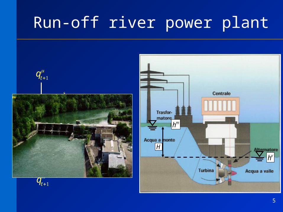
Run-off river power plant

qt+1m

qt+1v

qt+1d

qt+1r

Gt+1

Hvh

mh

qt+1m

qt+1d

45o

qmin

qmax

Hvh

mh

6

Run-off river power plant:causal network

qt+1m

ut

qt+1r

qt+1d

qt+1v

Gt+1

qt+1m

qt+1v

qt+1r

qt+1d

Gt+1

Maximum divertable flow qmax

MEF downstream qt

DMV

7

Run-off river power plant: mechanistic model

qt+1d =

0 if qt+1m −qt

MEF( ) < qmin

min ut, qt+1m −qt

MEF( )+,qmax

{ } otherwise

⎧

⎨⎪

⎩⎪

qt+1r =qt+1

m −qt+1d

qt+1v =qt+1

m

Gt+1 =ψ ηg g γ qt+1d H

qt+1m

ut

qt+1r

qt+1d

qt+1v

Gt+1

Energy production [kWh] in [t, t+1)

coefficient (/3.6 • 106)

η g turbine efficiency [-]

g gravity (9.81 m/s2)

γ water density (1000 kg/m3)

H hydraulic head (constant)

coefficient (/3.6 • 106)

η g turbine efficiency [-]

g gravity (9.81 m/s2)

γ water density (1000 kg/m3)

H hydraulic head (constant)

8

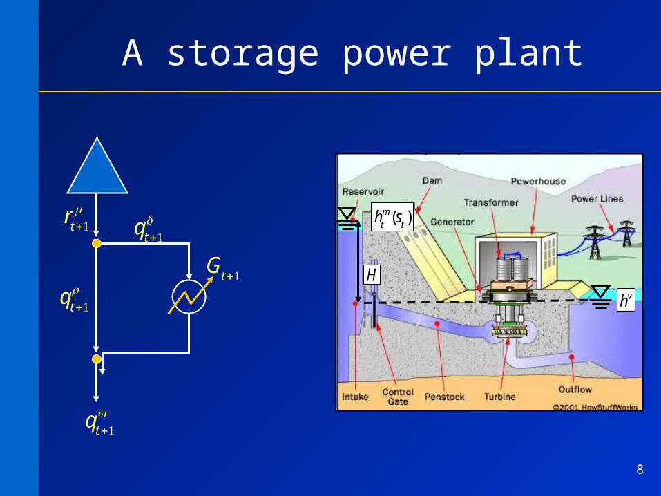
A storage power plant

qt+1m

qt+1v

qt+1r

qt+1d

Gt+1

rt+1m

Hvh

htm(s

t)

9

receiving water body

plant

reservoir

Storage power plantcausal network

rt+1m

qt+1r

qt+1d

qt+1v

Gt+1

1mtq

qt+1v

qt+1r

qt+1d

Gt+1

rt+1m

et+1m

utm

stm

htm

hv

at+1m

10

receiving water body

plant

reservoir

rt+1m

qt+1r

qt+1d

qt+1v

Gt+1

et+1m

utm

stm

htm

hv

Storage power plant mechanistic model

qt+1d =

0 if rt+1m −qt

MEF( ) < qmin

min rt+1m −qt

MEF( )+,qmax

{ } otherwise

⎧

⎨⎪

⎩⎪

qt+1r =rt+1

m −qt+1d

qt+1v =rt+1

m

Gt+1 =ψ ηg g γ qt+1d H

qt+1d =

0 if rt+1m −qt

MEF( ) < qmin

min rt+1m −qt

MEF( )+,qmax

{ } otherwise

⎧

⎨⎪

⎩⎪

qt+1r =rt+1

m −qt+1d

qt+1v =rt+1

m

Gt+1 =ψ ηg g γ qt+1d H

coefficient (/3.6 • 106)

η g turbine efficiency [-]

g gravity (9.81 m/s2)

γ water density (1000 kg/m3)

H hydraulic head

coefficient (/3.6 • 106)

η g turbine efficiency [-]

g gravity (9.81 m/s2)

γ water density (1000 kg/m3)

H hydraulic head

H =ht

m st( )−hv

11

Storage power plantmodel

qt+1d =

0 if rt+1m −qt

MEF( ) < qmin

min rt+1m −qt

MEF( )+,qmax

{ } otherwise

⎧

⎨⎪

⎩⎪

qt+1r =rt+1

m −qt+1d

qt+1v =rt+1

m

Gt+1 =ψ ηg g γ qt+1d H

H =htm st( )−hv

It’s a non-dynamic model

It’s a non-dynamic model

12

P

SG

M

SL

MEF Fucino

MEF Vomano

PIAGANINI

CAMPOTOSTO PROVVIDENZA

VILLA VOMANOIrrigation district(CBN)

P_pomp

SG+P_pomp

Water works Ruzzo

MEF Montorio

Schema logico corretto(centraliPR)

13

Reversible storage power plant

Reversibile: the power comes from the grid, the alternator works as engine for the turbines, which run in inverse mode and pump the water back to the upstream reservoir.

14

Reversible storage power plant

Only pumping, two distinct power plants

qt+1v

qt+1p

Gt+11

mtq

rt+1v

Downstream reservoir

Upstream reservoir

15

Pumping plantcausal network

qt+1v

qt+1p

Gt+11

mtq

rt+1v

Downstream reservoir

Upstream reservoir

downstream reservoir

plant

upstream reservoir

rt+1v

qt+1p

qt+1v

Gt+1

qt+1pot

rt+1m

htm

htv

et+1v

stv

εt+1p

stm

Energy supplied by the network during the night

Energy supplied by the network during the night

Flow rate potentially liftable The effective flow rate depends upon

• penstock capacity

• maximum upstream storage

• flow available for pumping downstream as a function of the water available

(s m −stm)

qmax

16

Pumping plantcausal network

qt+1v

qt+1p

Gt+11

mtq

rt+1v

Downstream reservoir

Upstream reservoir

downstream reservoir

plant

upstream reservoir

rt+1v

qt+1p

qt+1v

Gt+1

qt+1pot

rt+1m

htm

htv

et+1v

stv

εt+1p

stm

qt+1pot =εt+1

p / ψ η p g γ htv st

v( )−htm st

m( )( )

rt+1v =Rt

v stv,qt+1

pot,rt+1m ,et+1

v( )

qt+1p =min qt+1

pot,rt+1v ,(sm−st

m),qmax{ }

qt+1v =rt+1

v −qt+1p

Gt+1 =ψ η p g γ qt+1p h st

v( )−htm st

m( )( )

qt+1pot =εt+1

p / ψ η p g γ htv st

v( )−htm st

m( )( )

rt+1v =Rt

v stv,qt+1

pot,rt+1m ,et+1

v( )

qt+1p =min qt+1

pot,rt+1v ,(sm−st

m),qmax{ }

qt+1v =rt+1

v −qt+1p

Gt+1 =ψ η p g γ qt+1p h st

v( )−htm st

m( )( )

Upstream active storageUpstream active storage

17

Power plantstep-indicator

The step-indicator Gt(•) is the energy produced (or comsumed for the pumping plant): it is a physical indicator.

Sometime an econimic indicator might be preferable:

• income

• availability to pay

• social cost

Cost Benefit Analysis is usually adopted

Can be obtained by manipulating Gt(•) appropriately.

Can be obtained by multiplying

Gt(•) per the energy price (which

can be a function of Gt(•)).

18

Average annual revenueHyd1

M €

year

⎡

⎣⎢

⎤

⎦⎥

Indicators Hydropower revenue

Hyd1=

1N

Rt(G(qtd))

t∈H∑

Time interval WinterSumm

er

August + Sat

and Sun

00:00-06:3006:30-08:3008:30-10:3010:30-12:0012:00-16:3016:30-18:3018:30-21:3021:30-00:00

25.346.7

116.346.746.7

116.346.725.3

25.346.746.746.746.746.746.725.3

25.325.325.325.325.325.325.325.3

Energy prices (€/Mwh)Energy prices (€/Mwh)

Rt(E

c(q tc )

)

energia prodotta (Mwh/die)

va

lore

(M

il E

uro

)

Fascia F1 Fascia F2 Fascia F4

Ec(q

tc )

19

Irrigation district

20

P

SG

M

SL

MEF Fucino

MEF Vomano

PIAGANINI

CAMPOTOSTO PROVVIDENZA

VILLA VOMANOIrrigation district(CBN)

P_pomp

SG+P_pomp

Water Works Ruzzo

MEF Montorio

Schema logico corretto(centraliPR)

21

The irrigation districtThe most natural indicator for an irrigation district is the harvested biomass (harvest) or the lost harvest with respect to the potential harvest: from both one can easily obtain the economic return associated to the agriculture production

not easily

computable! not easily

computable!

Proxy indicator: average annual potential damage from the stress

f (•) is the potential damage;

Fa is the maximum stress occurred in the year a

iirr=

1N

f (Faa=1

N

∑ )

F

a=max

t∈a

1δ

Wτ −qτ( )+

τ =t−δ

t

∑water demand at time t

it depends on field capacity

water supply at time tdeficit at time t

It is not separable!Enlarge the state!

It is not separable!Enlarge the state!

!!

The model of the irrigation district must provide the water demands Wt for all the crops at time t.

The model of the irrigation district must provide the water demands Wt for all the crops at time t.

22

Not always such a simplified model is acceptable.

For instance:

If for several days a crop is not irrigated, the water demand becomes greater than that of regularly irrigated crop.

The irrigation district is a dynamic system.

If at the beginning of the year farmers decide to plant dry crops, the water supplied would not have any influence on the harvest.

The harvest depends on human expectations and decisions.

• crop characteristics;

• irrigation system;• current agricultural practice in the area.

The simplest way is to rely on an expert estimating the water demand scenario on the basis of: W0

T−1

How to determine the water demand Wt ?

23

Not always such a simplified model is acceptable.

For instance:

If for several days a crop is not irrigated, the water demand becomes greater than that of regularly irrigated crop.

The irrigation district is a dynamic system.

If at the beginning of the year farmers decide plant dry crops, the water supplied would not have any influence on the harvest.

The harvest depends on human expectations and decisions.

• crop characteristics;

• irrigation system;• current agricultural practice in the area.

The simplest way is to rely on an expert estimating the water demand scenario on the basis of: W0

T−1

How to determine the water demand Wt ?

The expert’s estimate is a description of the water demand in normal conditions, including a normal water supply.

It’s an accurate model for small variations in the water supply.

It’s not acceptable when variations are significant, such as:

• during exceptional droughts;

• when a change in the status quo is planned.

What can we

do else?What can we

do else?

24

Irrigation system-soil-vegetation (SSV) model

25

Irrigation system-soil-vegetation (SSV) model

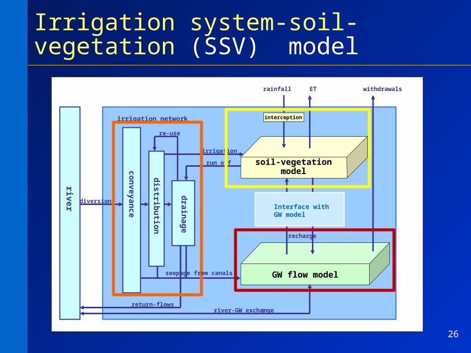
26con

veyan

ce

dra

inag

e

soil-vegetationmodel

GW flow model

Interface with GW model

river

irrigation

rainfall ET withdrawals

run off

recharge

river-GW exchange o

re-use

return-flows

diversion

irrigation network interception

dis

tribu

tion

Irrigation system-soil-vegetation (SSV) model

seepage from canals

27

rootzone

CANOPY INTERCEPTION: Hoyningen-Hune (1983), Braden (1985)

RAINFALL ANDIRRIGATION

INFILTRATION: Green&Ampt model (1911)or CN-SCS method (1972)

EVAPORATION: FAO-56 Allen et al. (1998)

TRASPIRATION: FAO-56 Allen et al. (1998)

PERCOLATION: RESERVOIR CASCADE(DARCY FLUX WITH UNIT VERTICAL GRADIENT)

CAPILLARY RISE PROCESSES

16560

cells16560

cells

28

Groundwater flow model (map of aquifer trasmissivity)

29

Example of output: irrigation supply

30

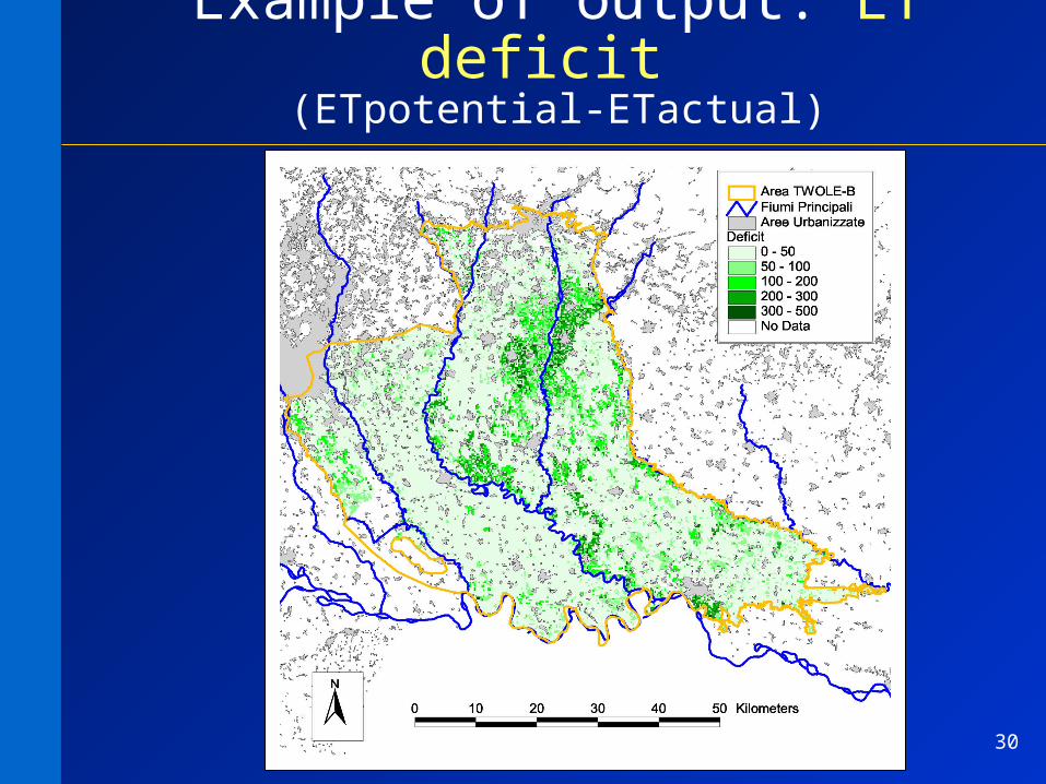
Example of output: ET deficit (ETpotential-ETactual)

31

Example of output: crop production index

32

Single cell outputs (daily time-step)

0

2

4

6

8

10

12 0

50

100

150

200

250

300

350

400

Maize cell in MulazzanoGW recharge

ETa

rainfall + irrigation

3333

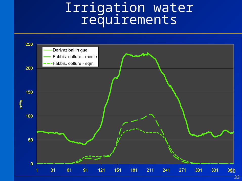
Irrigation water requirements

34

Irrigation district:the farmers’ behaviour

It is not always so easy!

35

The Vomano Project

The Consorzio di Bonifica Nord (CBN) would like to assess the opportunities for extending its irrigation district from 7000 ha to 14 000 ha.

Therefore CBN needs an estinmate of the water demand for the enlarged district.

CBNIrrigation district

36

Irrigation district: block diagram

extension

expectation

incentives

supply to the

districtt

temperaturet

solar radiationt

precipitationt

irrigation district

37

Distribution Growth

W

ti{ }

i=1

n

biomass

tr

i{ }

i=1

n

=harvest

biomass

ti ,moisture

ti{ }

i=1

n

crop areas

supplyt

Irrigation district: block diagram

extension

expectation

incentives

supply to the

districtt

temperaturet

solar radiationt

precipitationt

Potential Evapotransp.

irrigation techs.

Farmers Causal net

38

The farmers’ behaviour:causal network

extension expectation incentives

S % micro

extension expectation incentives

St &m

% microt&m S % microcau

Scau

Choice between:- dry crops and 1 irrigated crop- sprinklers and microirrigation

Choice between: - dry crops and 2 irrigated crops (cauliflower + tomato&maize)- sprinklers and microirrigation

39

Distribution Growth

W

ti{ }

i=1

n

biomass

tr

i{ }

i=1

n

=harvest

biomass

ti ,moisture

ti{ }

i=1

n

crop areas

supplyt

Irrigation district: causal network

extension

expectation

incentives

supply to the

districtt

temperaturet

solar radiationt

precipitationt

Potential Evapotransp.

irrigation techs.

Farmers BBN

40

Choice between: - dry crops and 2 irrigated crops (cauliflower + tomato&maize)- sprinklers and microirrigation

incen

tives

0

S

7000expectation

14000

7000

3500

10500

14000

0.9

0.7

0.5

0.1

0.3

0.5

0

0.40.1

0.1

0.1

0.1

0.4

0.4

0.3

0.3

0.1

0.5

0.2

0 0

0

0

0

0

0 0

0 0 0

extension

LO

W

AL

TA

ME

DIU

M

LO

W

HIG

H

ME

DIU

M

expectation

The farmers’ behaviour:Bayesian Belief Network (BBN)

extension expectation incentives

St &m

% microt&m S % microcau

Scau

constraint violation

41

Choice between: - dry crops and 2 irrigated crops (cauliflower + tomato&maize)- sprinklers and microirrigation

The farmers’ behaviour:Bayesian Belief Network (BBN)

extension expectation incentives

St &m

% microt&m S % microcau

Scau

0-50t&m

51-100

extension

7000

incentives

14000

incentives

0.9 0.7 0.5

0.1 0.3 0.5

0.9 0.7 0.5

0.1 0.3 0.5%micro

NO

NE

HIG

H

LO

W

NO

NE

HIG

H

LO

W

42

Choice between: - dry crops and 2 irrigated crops (cauliflower + tomato&maize)- sprinklers and microirrigation

The farmers’ behaviour:Bayesian Belief Network (BBN)

extension expectation incentives

St &m

% microt&m S % microcau

Scau

0

S

S

3500

7000

10500

14000

0

0

0

0

0

0

0

0

0 0

0

0

0

0

0

0

0

0

0

0

0

0

0

0

0

0

0

0

0

0

0

0

0

0

0

0

0 0

00

1

1

1

1

1

1

1

1

1

1

1

1

1

1

1 1 1

0 0 0

0

1

0

1 1

0

0

0 0

0

0

0000000

00 0

0000

0 0 0 0 00 0 0 0 0 0 0 0 0 0

S S S

3500 7000 10500 14000S

cav

p&m p&m p&m p&m

43

Calibration of the BBN

The BBN parameters are the Conditional Probability Tables.

To calibrate the BBN we need to estimate their elements (CPT population).

Simple algebraic relation: Scav = S - Sp&m

extension expectation incentives

St &m

% microt&m S % microcau

Scau

44

Calibration of the BBN

extension expectation incentives

St &m

% microt&m S % microcau

Scau

interviews

45

Distribution Growth

W

ti{ }

i=1

n

biomass

tr

i{ }

i=1

n

=harvest

biomass

ti ,moisture

ti{ }

i=1

n

crop areas

supplyt

Irrigation district: BBN

extension

expectation

incentives

supply to the

districtt

temperaturet

solar radiationt

precipitationt

Potential Evapotransp.

irrigation techs.

Farmers BBN SSV model

ALGEBRAIC model

FAO model

time t

46

t=0

t=1

t=T-1

...

Irrigation district: BBN

47

Model validation

flo

w r

ate

[m

3/s

]

canal capacity

model

real

48

The ecological status of a fluvial ecosystem

49

HIERARCHY

50

ECOLOGICAL STATUS

General conditions

Benthic macroinvertebrates

LIM

Biological quality

(terrestrial and aquatic biota)

Fish fauna

Terrestrial flora

Abundance

Biodiversity (EPT)

Community composition

Population structure (key species)

Autochthonous species

Exotic species

Age distribution structure

Abundance

Physico-chemical quality (water quality)

Riparian vegetation

Naturalness

Cover

Longitudinal continuity

Width of riparian strip

Corridor (zonal) vegetation

Hydromorphological quality Hydrological regime

Characteristics of regime (annual, monthly flows; max, min annual flow;

peak and period,…)Mean values

Standard deviations

Biodiversity-spring

Biodiversity-summer

Biodiversity-autumn

Biodiversity-winter

Total exotic species

Presence of Silurus Glanis

Naturalness of structural features

Autochthony

Naturalness (species)

Cover

Indicators not represented for lack of

space

HIERARCHY

51

Dissolved oxygen previous

3 months (d)

Median flow previous 3 months (Q)

Minimum flow previous month (q)

EVALUATION INDEX

Cause-effect relations

Pollutant loads reduction

Setting lake release policy and water distribution

policy

Stress hydromorphol.

conditions

Prevailing hydromorphol. conditions

Actions

Macroinvertebrates (m)

Biodiversity of the community (m1)

Abundance (of habitat) (m2)

Biodiv. winter (m11)

Biodiv. spring (m12)

Biodiv. summer

(m13)

Biodiv. autumn

(m14)

Causal factors

Macroinvertebrates: causal network

52

Median flow previous 3 months

(Q)

EVALUATION INDEX

Setting lake release policy and water distribution

policy

Macroinvertebrates (m)

Abundance (of habitat) (m2)

Flowrate

ActionsCause-effect relations

Wet area

Macroinvertebrates: causal network

53

Step 1 – Analysis of satellite images (Landsat TM 7)

Example 1 empirical, deterministic

model based on experimental data

Macroinvertebrates: determining cause-effect relationships

54

Step 2 - Classification and assignment of pixel “water”

Macroinvertebrates: determining cause-effect relationships

55

Step 3 – Estimation of the “flow rate-wet area” relationship

Macroinvertebrates: determining cause-effect relationships

y = 0,3397x + 30,406R2 = 0,8746

0

10

20

30

40

50

60

70

80

90

100

0,00 20,00 40,00 60,00 80,00 100,00

Flow rate [m3/s]

% W

et

su

rfa

ce

Real

Linear regression

56

FISH FAUNA (f)

Community composition (f1)

Abundance key species (f22)

Longitudinal Continuity

(l)

Prevailing flow during minimum flow quarter (Q)

Minimum daily flow during hatching

period key species (s)

EVALUATION INDEX

Creating fish-passages / removing

discontinuities

Setting lake release policy and water

distribution policy

Stress hydromorphol.

conditions

Prevailing hydromorphol.

conditions during minimum flow

period (same year)

Presence of autochthonous

species (f11)

Presence of exotic species (f12)

Age distribution structure key species (f21)

Population structure (key species) (f2)

Minimum annual

3-days flow (q)

Stress hydromorphol. conditions hatching period key species

Prevailing hydromorphol.

conditions during minimum flow period (last 3

years)

Exotic species / tot (f121)

Presence of silurus

(f122)

Actions

Causal factors

Triennial average of prevailing flow during

minimum flow quarter (m)

Cause-effect relations

Fish fauna: causal network

57

FISH FAUNA (f)

Community composition (f1)

Longitudinal Continuity

(l)

EVALUATION INDEX

Cause-effect relations

Creating fish-passages / removing

discontinuities

Setting lake release policy and water

distribution policy

Presence of autochthonous species (f11)

Prevailing hydromorphol.

conditions during minimum flow

period (last 3 years)

Actions

Causal factors Triennial average of prevailing flow

during minimum flow quarter (m)

Example 2 model based on expert judgment

Fish fauna: determining cause-effect relationships

58

For a given longitudinal stretch ...

Briglia diBriglia di RivoltaRivolta

Presa Canale VacchelliPresa Canale Vacchelli

Briglia diBriglia di SpinoSpino

Briglia di LodiBriglia di Lodi

Briglia di Briglia di PizzighettonePizzighettone

Soglia di Soglia di MaccastornaMaccastorna

Sbarramento con passaggio per pesci non funzionanteSbarramento con passaggio per pesci non funzionante

Sbarramento sprovvisto di passaggio per pesciSbarramento sprovvisto di passaggio per pesci

Non valicabile in condizioni di portata di magra

Briglia diBriglia di RivoltaRivolta

Presa Canale VacchelliPresa Canale Vacchelli

Briglia diBriglia di SpinoSpino

Briglia di LodiBriglia di Lodi

Briglia di Briglia di PizzighettonePizzighettone

Soglia di Soglia di MaccastornaMaccastorna

Sbarramento con passaggio per pesci non funzionanteSbarramento con passaggio per pesci non funzionante

Sbarramento sprovvisto di passaggio per pesciSbarramento sprovvisto di passaggio per pesci

Non valicabile in condizioni di portata di magra

Fish fauna: determining cause-effect relationships

59

?

?

?

?

?

CORNATE - reali

0

100

200

300

400

500

600

700

800

900

23/12

/1989

07/01

/1990

22/01

/1990

06/02

/1990

21/02

/1990

08/03

/1990

23/03

/1990

07/04

/1990

22/04

/1990

07/05

/1990

22/05

/1990

06/06

/1990

21/06

/1990

06/07

/1990

21/07

/1990

05/08

/1990

20/08

/1990

04/09

/1990

19/09

/1990

04/10

/1990

19/10

/1990

03/11

/1990

18/11

/1990

03/12

/1990

18/12

/1990

02/01

/1991

1990 reale

1991 reale

1992 reale

1993 reale

1994 reale

1995 reale

Qmin flow quarter

Hydromorphol. conditions (v, h, t...)

Fish fauna: determining cause-effect relationships

60

f11(sc.A)

0

4

8

12

16

20

24

5 24 43 62 81 100

m [m 3/s]

IF 5 < m ≤ 25 → f11 = 6 + (8/20)*(f11-5)*m;IF 25 < m ≤75 → f11= 14 + (5/50)*(f11-25) *m;IF m > 75 → f11 = 19

X

X

Fish fauna: determining cause-effect relationships

61

DisturbancesThe disturbances is so with respect to the component we are considering.

It could be described by a modelas a function of other variables or its own past values.

For example:

at+1

at+1

The focus is now on the system.

When the disturbance of a component is explained with a model, it is an internal variable of the system.

The new “candidate” disturbance is the disturbance of the new model.....

Pt+1

.... the sequence ends when all the disturbance to the global model are either deterministic or random.

.... However also this latter could be described with a model....

62

DisturbancesTherefore:

The disturbance of a component is also a disturbance for the global model if and only if:

It does not need to be “explained” through a model: it is a deterministic variable;

It cannot be “explained” through a model: it is a purely random variable.

Just check if its value is deterministically know at each time instant. Whiteness test

63

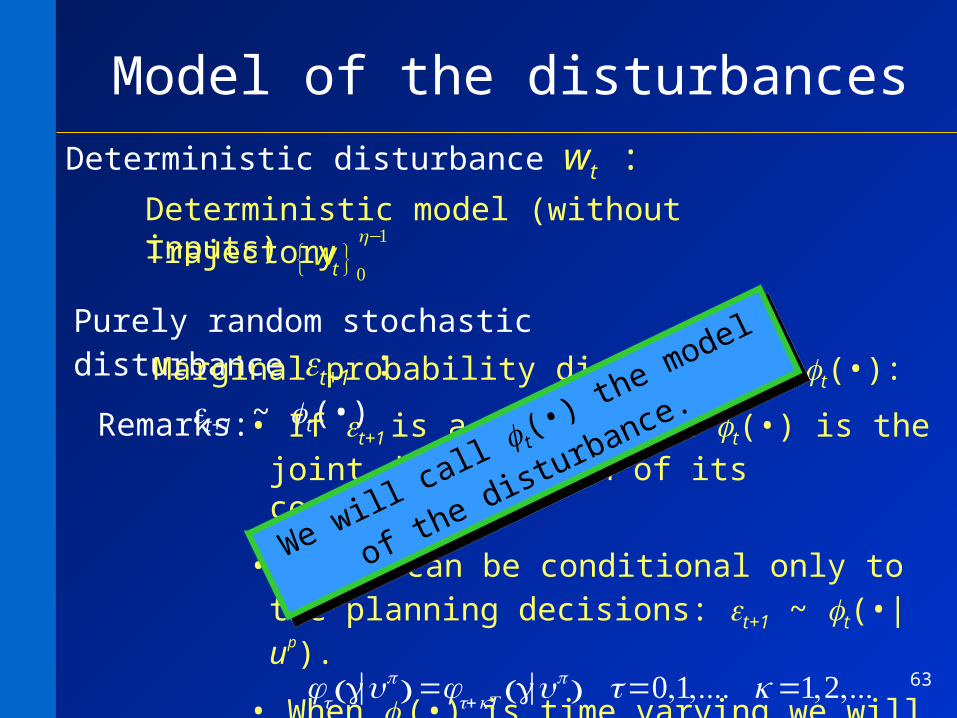
Model of the disturbances

Deterministic model (without inputs)Trajectory

w

t{ } 0h−1

Deterministic disturbance wt :

Purely random stochastic disturbance εt+1 :Marginal probability distribution t(•): εt+1 ~ t(•)

φt g|up( ) =φt+kT g|up( ) t=0,1,.... k=1,2,...

• If εt+1 is a vector then t(•) is the joint distribution of its components.

• t(•) can be conditional only to the planning decisions: εt+1 ~ t(•|u

p).

• When t(•) is time varying we will assume it as periodic

Remarks:

We will call t(•

) the model of th

e

disturbance.

We will call t(•

) the model of th

e

disturbance.

64

Model of the disturbances

Purely random uncertian disturbance εt+1 :The knowledge is not enough neither to express a probability t(•);

We only know that the disturbance values belong to the data interval t: εt+1 t

t up( ) =t+kT up( ) t=0,1,.... k=1,2,...

• t can only depens upon the planning decisions: t (u

p).

• When t is time variant we can assume it as periodic:

Remarks:

We will call t th

e model of the

disturbance.

We will call t th

e model of the

disturbance.

65

Reading

IPWRM.Theory Ch. 5