BUREAU OF THE CENSUS

STATISTICAL RESEARCH DIVISION REPORT SERIES

SRD Research Report Number: CENSUS/SRD/RR-88114

OUTLIERS IN TIME SERIES

J. Peter But-man Mark C. Otto University of Kent Statistical Research Division

at Canterbury Bureau of the Census Canterbury, England Washington, D.C. 20233

This series contains research reports, written by or in cooperation with staff members of the Statistical Research Division, whose content may be of interest to the general statistical research community. The views re- flected in these reports are not necessarily those of the Census Bureau nor do they necessarily represent Census Bureau statistical policy or prac- tice. Inquiries may be addressed to the author(s) or the SRD Report Series Coordinator, Statistical Research Division, Bureau of the Census, Washington, D.C. 20233.

Recommended by:

Report completed:

Report issued:

Nash J. Monsour

May 18, 1988

May 20, 1988

CENSUS BUREAU RESEARCH PROJECT

OUTLIERS IN TIME SERIES

bY

J. Peter Burman

and

Mark C. Otto

.

* J. Peter Burman is an honorary professor at the Mathematical Institute, University of

Kent, Canterbury, Kent, CT2 7NF, England and Mark C. Otto is a Mathematical

Statistician with the Statistical Research Division of the Census Bureau, Washington, DC

20233. This paper is based upon work supported by the National Science Foundation

under grant SES 84-01460, “On-site Research to Improve the Government-Generated

Social Science Data Base.” The research was conducted during September-December 1984

and July-September 1985, at the U.S. Bureau of the Census while the authors,

respectively, Research Fellow and Associate in the American Statistical

Association/Census Bureau Research Program. The.program is supported by the Census

Bureau and through the NSF grant. Any opinions, recommendations expressed here are

those of the authors and do not necessarily reflect the views of the National Science

Foundition or the Census Bureau. The authors would like to thank William R. Bell and

David F. Findley for their support and helpful suggestions.

2

ABSTRACT

We study the effects of outliers on short-term forecasting errors and on

autoregressive-integrated moving-average (ARIMA) model characteristics such as the

Ljung-Box statistics and estimates of the seasonal moving-average parameter. We have

fitted sixty Census Bureau monthly time series with ARIMA models, identified additive

point outliers, and sought their external causes. Modification of outliers was found not

increase the mean absolute forecasting error (of one, two, and three steps-ahead forecasts

over the last three years of the data) in 31 out of 44 series with identified outliers. We also

discuss consequences of different methods of outlier modification, choice of outlier

identification threshold, and effects on the seasonal adjustment of time series. *

KEYWORDS: Time Series; AR.IMA model; Outlier; Signal Extraction; Forecasting;

Seasonal adjustment; Census X-11.

3

1. OUTLINE OF PROBLEM

It is often taken for granted that modification of outliers improves the forecasting

performance of a time series model, because:

1. It is believed that outliers occur at places where the process generating the series

has temporarily broken down, so that modification of outliers is needed to

compensate for this in the forecasts calculations.

2. If so, modification should bring the parameter estimates closer to their true

values, resulting in improved forecasts.

In practice, this is far from clear. The threshold used to define outliers is arbitrary and for

a given threshold, when more data are used, the outlier set is often not the same. Also, if *

the innovations of the model-generating process are not Normal (but from a fat-tailed

distribution), the threshold may be detecting outliers more often than intended. In this

paper we study the empirical effect of outlier modification on post-sample forecast errors -

not those within sample, which are bound to be reduced.

Different types of outliers were defined by Fox (1972), and Denby & Martin (1979):

additive outliers (AO), which affect only a single observation, and innovative outliers (IO),

where an unusual innovation in the generating process affects all later observations.

Further types of outliers, which Pierce (1987) calls “mixed”, arise when only one

characteristic of the series (e.g. trend or seasonal component) is changed by the innovation.

In the context of seasonal adjustment, automatic outlier identification and modification

has been practiced for many years, e.g., in the Census X-11 program (Shisken, Young, and

Musgrave 1963). When seasonally adjusting with X-11, a series is decomposed into trend,

seasonal, and irregular components, regardless of the series generating process. Outliers are

identified from the irregular series, using a threshold which is a multiple of the root mean

square of an appropriate span of the series. But the default option, which is commonly

used, leads to a large proportion of outliers, perhaps 10 percent of the observations, and it

seems unlikely that the generating process has broken down so often. A further arbitrary

feature is the need to choose a moving average for the seasonal component (e.g. [3] [5] or [3]

[9]), which determines what the irregular series looks like.

Hillmer, Bell, and Tiao (1983) (hereafter called HBT) and Bell (1983) applied a more

rigorous approach to the treatment of outliers in model-based seasonal adjustment. They

showed how the residual errors of the model can be used, with a given threshold, to identify

outliers of different types. Regression estimates of their magnitudes provide starting values

- in an extended model, which includes dummy variables to represent the outliers. Burman

(1983) indicates, for the simpler models, the link with the traditional outlier+letection

method of X-11.

In this paper, the full HBT method is called “simultaneous estimation” of outliers: it is *

an extension of Intervention Analysis - see Box and Tiao (1975). In our view, unless

external causes can be identified, this extension suffers from the conceptual difficulty that

the hypothesis being tested has an indefinite number of parameters. An alternative

considered here is to use the regression estimates of the outliers, as they stand, to modify

the series, and then refit the original model.

Another question is the effect of outliers on the quality of a seasonal adjustment. A

number of authors have suggested criteria for the quality of a seasonal adjustment

procedure, e.g., maximum smoothness of the seasonal component, sensitivity to change,

minimizing average revisions over the last few years - see HBT and Burman (1980). But

there is no agreement over the ranking of these criteria; in particular, for comparison of

revisions between X-11 and model-based adjustments, the methods are targeting different

final adjusted series. So we side-step the problem in this paper by concentrating on

short-term forecasting performance of a fitted model, since this is often the main purpose

of seasonal adjustment.

5

2. IDENTIFICATION OF OUTLIERS

HBT showed that outliers could be identified in a way not involving decomposition into

trend, seasonal, and irregular. Assume that the current observation zt (if necessary,

transformed) can be expressed as a weighted average of past values plus an innovation

which is Normally distributed white noise: i 1. zt = at - 7r1zt-1 - 7r2ztB2 1.. or

(l+rlB + 7r2B2 ..- )zt = at, where Bzt = zt-I, We write this as: 7r(B)zt = at. The series

of coefficients is infinite, unless the model is purely autoregressive.

Following Denby and Martin (1979), HBT classify two types of outliers: additive (AO)

and innovative (IO). An IO at time t6 affects the innovation at and is built into the future

level, slope, and seasonality of the series; it is estimated directly from the innovation. An *

isolated A0 at time t only affects zt itself and not future values zt+k’ But it produces a ,. ,.

large forecast error at and this affects future forecast errors at+k to a diminishing extent.

Bell (1983)etending the outlier procedure in HBTidentifies two other types of

outliers affecting the zt series, changes in level and changes in the seasonal pattern.

Changes in level can be treated as isolated AO’s in the differenced series, AZ+,, and changes

in the seasonal pattern can be treated as AO’s in the seasonally differenced series, A12zt.

HBT show that the best estimate of an A0 outlier magnitude, or(t), in a series of length n * I A

is obtained from a linear regression of the at, at+l, ..., and a, on the r-weights t. ,. 0. I

4’) = (at+Tlat+1+T2at+2+ ‘*. *n-t a n )/(l+rT+ri+ ... &). Now, define the

numerator as It and the denominator as wn * t. if the threshold for an outlier is a constant *

multiple of the standard error of It, it tapers quite sharply downwards as t approaches n. ,. ,.

If the at are estimates of independent Normal variates, the It are Normal and can be given

a t-test. The at are unknown beyond t = n, but their expected values are 0. So we can ,. * L) ,.

write It = “(F)at , where Fat = a t+l, the inverse operator to B. In the discussion on

HBT, the first author pointed out that, providing t is not too small, 4B)zt = at, and I, ,.

can be written in a symmetric form: It = z-(F)lr(B)zt. This is to be understood as a

6

doubly infinite moving average, in which missing values are replaced by forecasts and

backcasts, and the technique of Signal Extraction will evaluate it--see Burman (1980).

If (n-t) is not small (in practice more than 2 years), wt is almost equal to w =; 2. aI i=O ’

So the threshold for an outlier is proportional to w l/2 . tD m the central part of the series. By

the symmetry of It, the threshold must also taper near the start of the series. To see how

this happens, we note that the same model can be expressed in terms of the backcast A

errors, et: rr(F)zt = et and hence It = Ir(B) So, for small t, the threshold is

t 2 l/2 proportional t0 Wt = { C “i } .

i=O

If several outliers are tentatively identified, a multiple regression gives estimates which

allow for interactions between any that are close together. For example; if there are *

outliers at t and (t+2), the forecast errors have not recovered from the first shock before

the second one is upon them. Interaction also occurs for monthly seasonal series with

outliers at t and (t+12). For detailed formulae, see the Appendix.

We automatically identify and estimate modifications for outliers using an iterative

process similar to HBT:

(1) Calculate a robust version of the root mean square error (RMSE) of at.

(2) Estimate it and the the threshold values (w:/t.RMSE) and identify, using a

t-statistic, all those values beyond their thresholds.

(3) Re-estimate the effects of the all the outliers-including the newly identified ,.

out liers -using a multiple regression. Then revise It, the RMSE, and the threshold

values, using the residuals from the outlier regression. If this is the first pass,

replace the robust RMSE by the regression RMSE.

(4) Repeat (2) and (3) until no more outliers are found.

(5) Do backward elimination (Draper and Smith 1981, pp. 305-307) of outliers until

only outliers with t-statistics over the threshold remain.

(6) Estimate modifications for time points that have It values between a partial outlier

threshold and the full outlier threshold.

As does Bell (1983), we use a robust version for the initial RMSE estimate (in (1)).

W.S. Cleveland in his discussion of HBT pointed out that the initial estimate of aa will be

biased upwards if the series contains several large outliers. Practically, we may fail to

detect any outliers on our initial pass over I, because of this misspecification of the RMSE.

Bell adopted Cleveland’s suggestion to use 1.48*median 1 at 1 which is based on the relation

between the quartiles and the standard deviation of the Normal distribution. We use this

‘only for the initial pass over It, then after an initial set of outliers has been identified we

use the parametric RMSE. .

The*backward elimination procedure is used in (5) because of situations such as

“shadows”. It often happens that a large outlier is not identified on the first pass but has

an adjacent shadow (of opposite sign) which is identified. When the two are in the outlier

regression together, the shadow drops out.

Finally, in (6), because of the uncertainty over identification of outliers, irregularities

with t-values between the partial outlier threshold and the full outlier threshold (2.5 to 3.0

in our study) are treated as partial outliers (as in X-11). The amount of modification is

determined linearly by the value of I, and the position of the t-statistic between the

thresholds, so o(t), as defined above is multiplied by (t-2.5)/(3.0-2.5). Partial outliers

modifications are not estimated in the regression (steps (2) and (3)) and their modifications

do not affect the value of the RMSE used to detect other outliers.

Bell (1983) not only identifies and adjusts for point (AO) outliers but also changes in

level and changes in the seasonal pattern. He tests for these three types of outliers

simultaneously at each time point and chooses the most probable type or combination of

types. We identified such outliers by looking at the irregular of the differenced series.

8

After tentative identification, two alternatives are open:

(1) Modify the series, using the regression estimates for the outliers, and refit the

model.

(2) Introduce dummy variables to represent the outliers and re-fit the extended model.

The second is the one adopted by Bell (1983). He has an outer iteration loop as well,

returning to outlier identification after the re-fit, and repeating until no more outliers are

found. In our work, this outer loop was omitted, but both (1) and (2) were tried. Also

automatic identification was only used for isolated AO’s. Step changes were identified

from the irregular of the differenced series and added to the model manually and IO

ident&ation was not attempted.

3. SERIES DESCRIPTIONS

60 Census Bureau monthly series were modeled: 17 Business Division retail and

wholesale sales series, 15 Construction Division housing start and building permit series, 9

Foreign Trade Division import and export series, and 19 Industry Division value shipped,

total inventory, and unfilled orders series (see Table 1). They are by no means a random

sample, but consist mainly of series used by HBT, plus some Foreign Trade series already

analyzed by members of the Statistical Research Division at the Census Bureau. The

Retail Sales of Services series used by HBT have been discontinued. Most series were

updated to 1982, though some ended in 1981 or 1983. The aim was to obtain 20 years’

data, except for Business Division, whose series began in 1967.

9

4. MODEL IDENTIFICATION

Models were identified initially from the autocorrelations (ACF) and partial

autocorrelations (PACF) of zt (the logarithm of the original series), Azt, A12zt, and

AA12zt. For series where Trading Day (TD) effects are suspected, a 3-term periodicity in

the ACF will usually be noticed, with r4, r7, and rIO being prominent. This can be tested

by a regression of AA12zt on differenced TD variables (see HBT), and model identification

based on the residuals of this regression.

We estimate the models using Burrnan’s (1980) exact likelihood estimation and signal

%xtraction program. If the initial model is over-parameterized, the estimation program

automatically reduces it, e.g. canceling a common factor between AR an’d MA, reducing

the orier of AR or MA, changing an AR factor into a difference, or replacing moving

seasonality by fixed seasonal means. However, experience showed that it is prudent not to

reduce the order of AR or MA (non-seasonal) until re-estimation after outlier

identification. Also, even if the first estimation gave a fixed seasonal pattern, a moving

pattern was tried again on re-estimation (see Section 8). With these exceptions, the same

model was fitted on both estimations.

Model choice was also influenced by its potential use for seasonal adjustment. The

optimal linear filters to extract the Trend, Seasonal, and Irregular are derived from the

decomposition of the model spectrum (or pseudo-spectrum, when the model is

non-stationary) - see Box, Hillmer, and Tiao (1978) and Burman (1980). Not all models

have a valid 3-way decomposition, i.e. one with non-negative spectra; and, when two

models fit equally well, one with a valid decomposition and monotonic Trend spectrum (i.e.

most power at low frequencies) is preferred. These criteria tend to conflict: the second

leads to a preference for MA rather than AR models, but sometimes the former have only a

valid 2-way decomposition (i.e. seasonal and non-seasonal). If there is no valid

decomposition at all (which can occur with models which cannot be factorized into seasonal

10

and non-seasonal parts), the model is rejected.

The final choice of models included [23] (0 1 l)(O 1 1)12 models, [6] others with 1 or 2

ARMA parameters, [20] with 3, and [lo] with 4 or 5 parameters (see Table 2). In many

cases the number of parameters was reduced by constraining insignificant ones to zero.

The numbers quoted exclude the seasonal means, in cases where there is a fixed pattern.

5. DESIGN OF THE PROJECT

* For each series, the last 36 observations were truncated, the chosen model fitted, and 3

post-sample forecasts made (the unadjusted or U estimates). Then outllers were identified

(irregularities with t-values > 3), the series modified, the model re-fitted, and another set

of forecasts made (the modified outlier or MO estimates). Then 3 observations were added

to the series, and the process repeated 11 more times. At the 13th step, the full series was

modeled and modified for outliers, to provide “actuals” for comparison: forecasts cannot be

expected to anticipate an outlier. We call the results a chain run. The logarithms of all

the series were modeled to stabilize the variance, and because the series were transformed,

the comparisons of the forecasts were done in terms of the logarithms to avoid bias.

It seems to the authors that HBT’s simultaneous estimation of outliers, although

appealing as an ‘optimal’ solution, needs to be treated with caution. A model hypothesis

should have a definite number of parameters, determined by an objective criterion, e.g. the

AIC, whereas the number of outlier dummies depends on the threshold chosen. Moreover,

if an outlier is close to the threshold (e.g. t-value < 3.5 with a threshold of t=3), it may

not be identified on all the steps of the chain (“consistently identified”). The authors

believe that it is better to try to assign external causes to identified outliers, and to confine

the introduction of dummy variables to these cases; in fact, we were only partially

successful in this quest, and some large outliers whose causes remain unknown were

11

consistently identified. We re-estimated the chain runs with dummies for both the

externally caused and consistently identified outliers: the corresponding forecasts are

denoted SO (simultaneous outliers).

6. NATURE OF OUTLIERS

In attempting to link the identified outliers with external causes, two main sources were

used. The first was the Chronology of Recent Noteworthy Events (1962-1984), compiled

by the U.S. Bureau of Economic Analysis. It is a monthly economic memorandum that

reports on major strikes and other economic and political events that effect the U.S. *

economy. This information was followed up by contacts with the Bureau of Economic

Analysis and some market research firms in looking at particular industries. The second

source was the monthly averages of temperature and precipitation recorded by the National

Oceanic & Atmospheric Administration (NOAA). With one exception-the step change

in the Variety Stores series discovered by HBT-only simple A0 outliers were confidently

identified; though there may have been a step change in the seasonality of the inventories

of Oils and Fats (IFATTI). The absence of trend level changes is probably due to the

Census Bureau’s policy of adjusting backwards for known changes in data collection.

Abrupt changes in seasonal pattern do not occur if it is caused by weather or custom. The

identification of causes is discussed by Divisions (also see Table 2). ,

1. Business Division (19 outliers). These are very smooth series, only 9 out of 17

having any outliers (at t-3). All the series show Trading Day variation, but this is

partly an artificial effect, because roughly 30 percent of businesses report in 4- and

S-week periods, and Business Division adjust8 these figures to calendar months,

12

using the estimates of X-11 TD effects for those firms which do report in calendar

months. For 7 outliers, external causes have been identified: unusually cold

weather in the Northeast and North Central Regions, and a massive drop in the

level of sales by Variety Stores in 1976, due to the closing down of W. T. Grant

(noticed by HBT). A further 8 outliers are consistently identified, all with t-values

below 4.

- 2. Construction Division (59 outliers). Most of these series are straightforward to

model, because their noisiness submerges any complex correlation structure. The

. outliers were predominantly negative and 45 out of 59 were in the months of

December-February: the prime cause was exceptionally cold weather. NOAA * made available monthly averages of temperature and precipitation for various

sub-regions for 1963-73, and Mr. Goodman (Federal Reserve Board) provided

Census Region deviations from the lo-year averages for 1974-83, derived from

NOAA data. Precipitation seems to have no effect, but both Housing Starts and

Building Permits in the Northeastern and North Central Regions were affected by

unusual cold (and occasionally unusual warmth). We were able to connect 37 out of

44 consistently identified outliers with extreme weather, all except one in the

winter; the exception is a drop in CAOPVP in July 1977, the hottest July since

1932. However, the relation between temperature and irregularities in the series is

not very close: some extremely cold months were not outliers for any of the series,

and 5 out of 7 consistently identified outliers (4 negative) were in the months

March-June. A possible explanation is that mean daily temperature is not the

appropriate variable, but the number of days on which it is freezing at 8 a.m., and

so the workforce sent home-a suggestion made by Mr. Goodman.

13

3. Foreign Trade Division (33 outliers) Some of these series were hard to model, in

particular FUNKXU (Q jumped from 29 to 56 after outlier modification) and

FEECXU (the latter was dropped from the study for this reason). Causes for 19

outliers were identified and large outliers in 1969 and 1971 were found in all series,

except those for Canada. These were quickly identified from the Noteworthy Events

sheets as due to national dock strikes. One negative outlier was found in a

Canadian series in February 1967, which could be attributed to exceptionally cold

weather. A negative outlier in August 1977 in exports of raw materials was

probably due to a steel strike. One outlier.was consistantly identified (in FIRMXU)

* leaving 13 outliers, which were only identified on some runs and mostly did not

occur in the same month in different series, had &values less than 4. *

4. Industry Division (71 outliers). 34 of these could be linked with a variety of

external causes: strikes in the Glass Container industry in 1966 and 1968;

Communications Equipment affected by strikes at A.T.&T. in 1974 and 1983, and a

jump in shipments in December 1983 just before the corporation% reorganization;

the dip in Farm Machinery and Equipment shipments in October 1970, 1973, and

1976, when the 3-year labor contract at International Harvester was re-negotiated.

Inventories of Oils and Fats have outliers only in August-October, due to large

revisions to crop forecasts, just before harvest. Other causes of outliers include big

changes in interest rates, anticipated price increases, end-season discount sales,

unusual weather, and the first oil crisis in 1973. A further 18 outliers were

consistently identified, but with no obvious cause, leaving 21 which were only

identified on some chain runs.

14

7. RESULTS OF THE CHAIN RUNS

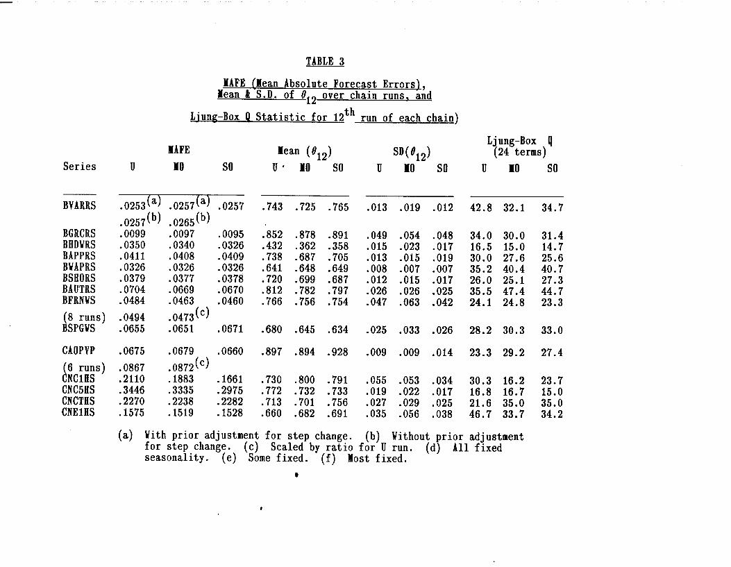
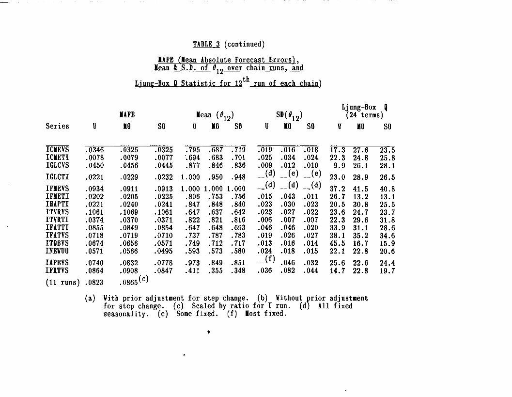
For the 45 series with identified outliers when the threshold is t=3, Table 3 shows the

mean absolute forecasting errors (MAFE) over the 36 post-sample forecasts, in natural

logarithms. The headings are U (unadjusted), MO (modified), and SO (simultaneous

outliers). In a few cases, when only a subset of the 12 runs of an MO chain contain

identified outliers, the MAFE(U) for the subset is also given, to enable comparisons to be

made with the MAFE(M0). The MAFE(S0) all refer to complete chains, because the

same outliers are specified on each run. The next-3 columns show the mean values of t912,

the seasonal MA parameter, over the 13 runs in each chain (including the full series); and

the next 3 columns give the standard deviation of $, over the 13 runs. ‘When any run has

012 ab&e 0.96, the program automatically switches to fixed seasonal means; these cases

are treated as if fl12 = 1 in calculating the means, but the SD columns are blank.

Table 4 gives a couple of examples of the variation in fl12 during a chain run. It is

difficult to draw general conclusions from these results. Table 5 summarizes the ratios of

the MAFE’s by Divisions: for 30 out of 45 series MAFE(M0) is less than or equal to

MAFE(U), but in only 8 cases does it exceed MAFE(U) by more than 1 percent (including

3 of the Industry Division Inventories series, which are known to be of lower quality than

Shipments). This suggests that outlier modification is usually worthwhile, and rarely

harmful. MAFE(S0) is also less than or equal to MAFE(U) for 30 out of 45 series.

However, only 9 of the remaining 15 are also MO failures. For 10 of the SO failures, the

MAFE exceeded the MAFE(U) by more than 1 percent. On the whole there seems little to

choose between the MO and SO methods of dealing with outliers: 23 series favor MO and

18 series SO, leaving 4 neutral. Simultaneous estimation takes longer, because it involves

more parameters; but, if the purpose is seasonal adjustment, the fact that the same outliers

are picked at each update should reduce the size of revisions.

15

8. INTERACTION BETWEEN FORECAST ERRORS,

OUTLIERS AND MODELS.

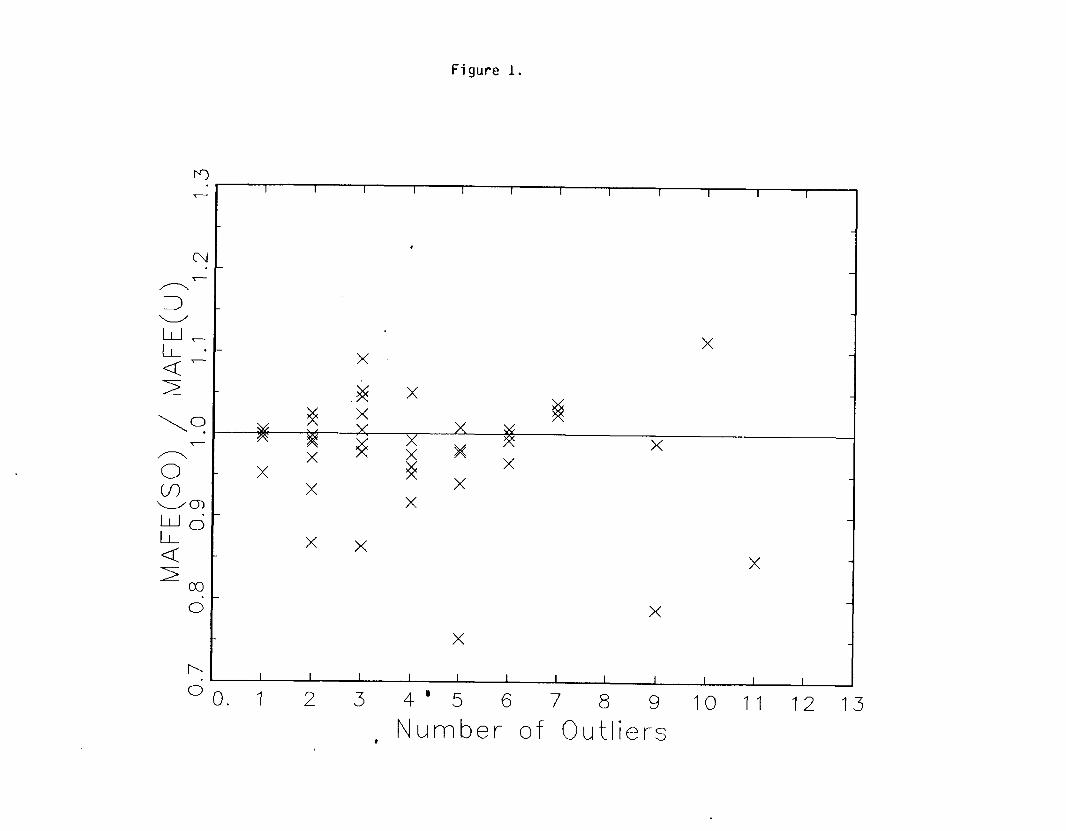
Is there any way of predicting the effect of outliers or model characteristics on the

MAFE? E.g. does the treatment of outliers become more important, as their number

increases? Figure 1 shows no correlation between the ratio MAFE(SO)/MAFE(U) and the

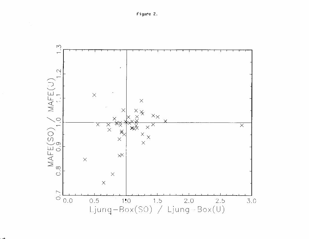
number of outliers. Does an improvement in model fit, after allowing for outliers, reduce

the MAFE? Apparently not-see Figure 2, which plots the MAFE ratio against the ratio

of the two Ljung-Box statistics for the 12th run of the chain: the correlation (0.241) is not

quite significant at the 10 percent level.

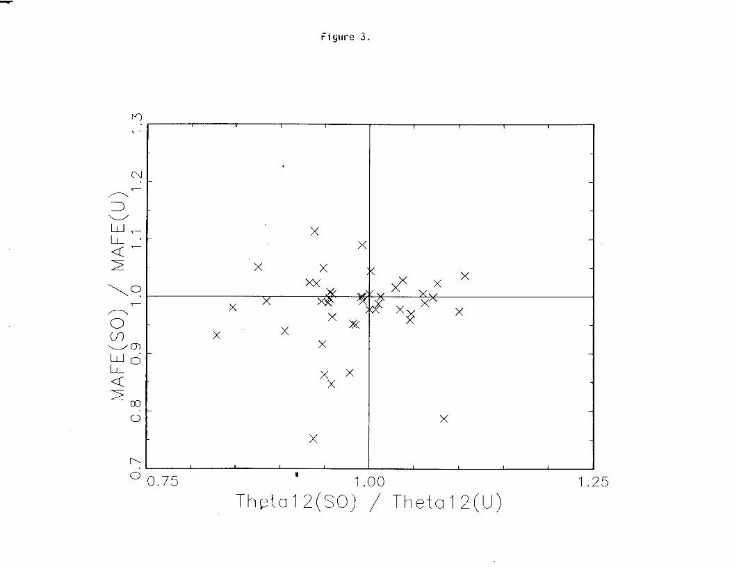
Finally, does the stability of the seasonal pattern give any information about the MAFE *

ratio? Outlier modification decreases 19 12 in almost three quarters of the series, i.e.

apparently the noise of the outliers had partially concealed a moving pattern. This is

always the case when e12(U) > 0.9, and usually when it exceeds 0.8; for several of these

series all runs of the U-chain give a fixed pattern, but many of the MO and SO runs

indicate slowly moving seasonality. The remaining quarter of the series, for which e12

increases on modification, suggest a model in which the presence of outliers has obscured

what was really a stable pattern. A priori, one would expect in the latter case

MAFE(MO)/MAFE(U) < 1. But our admittedly small sample shows no inverse

correlation between the MAFE ratio and the ratio of the corresponding mean values of 012

(see Figure 3). Finally we note that the Standard Deviation of e12 increased in 21 out of

45 series when using the SO method.

9. THRESHOLD

16

So far the threshold for full outliers has been taken as t-3, because that was the value

used by HBT. A limited amount of work was done with the threshold at k2.5, while

making no allowances for partial outliers. Summary results are shown in Table 6. For 3 of

the 60 series the number of identified outliers rose to more than 20 (the maximum that the

program can handle at the moment) in more than half the chain runs. For 36 series no

more outliers were identified; of the remaining 21, 15 favored the t=2.5 threshold and 6

supported the t=3 threshold. Clearly more work needs to be done in this area, but it is

unlikely that there will be overwhelming evidence against t=3.

10. CONCLUSIONS .

*

When using time series models for seasonal adjustment or short-term forecasting, the

treatment of outliers is of prime importance. Two methods are explored: (1) automatic

outlier identification and modification; (2) identification of external causes and

simultaneous estimation of outliers, using dummy variables. Of the 60 series examined, 45

had outliers at the t=3 threshold; and two thirds of these had smaller post-sample forecast

errors after allowing for the outliers. However, no characteristic (e.g. number of outliers,

goodness of model fit, stability of seasonal pattern) was found which would enable us to

predict whether outlier treatment will be beneficial for a particular series.

It seems that, in order to decide whether to ignore outliers in a particular case, we need

to hold out some of the data and calculate the post-sample forecast errors from a sequence

of runs. A priori, it is unlikely that we can afford to ignore identified outliers in the latest

year, even if the test suggests that the rest of the outliers should be ignored. However,

more research is needed, on a larger scale, to see whether the influence of an outlier on the

forecasts (both direct and through the parameter estimates) varies with its distance from

the end of the series.

17

Which of the two methods of outlier treatment is preferable is a matter of much less

importance: it may well be decided by the amount of statistical and economic expertise

available and the computer resources. Likewise the question of the choice of t-value for

the threshold is not crucial; but, until more research has been done, t=3 is recommended.

Another area for investigation is whether heteroscedasticity of the innovations process

between months (e.g. due to weather in Construction, harvest variations in Inventories of

Oils and Fats) should be incorporated in the Likelihood function.

Finally, what are the practical lessons for the seasonal adjusters? There is evidence that

the model-based method gives a “better” adjustment for some series (Bell and Hillmer

41984)), though X-11 may be satisfactory for many, perhaps the majority. It is

recommended that the model-based algorithm should be used initially as an adjunct to

X-ll:*first, to estimate 012 and so decide whether the 3x5 seasonal moving average should

be replaced by a less flexible smoother; second, to identify outliers and modify the series,

before X-11 is run.

APPENDIX

A.l. MODELLING ADDITIVE OUTLIERS

An additive outlier (AO) only affects the series at to:

e B Zt = dd at + d(t,t,) (A4

where [(t,t,) = (1 if t = to, and 0 otherwise) and 4(B) may contain difference operators.

Following HBT, but using slightly different notation, let ut be the innovations estimated

from the model without taking account of outliers.

18

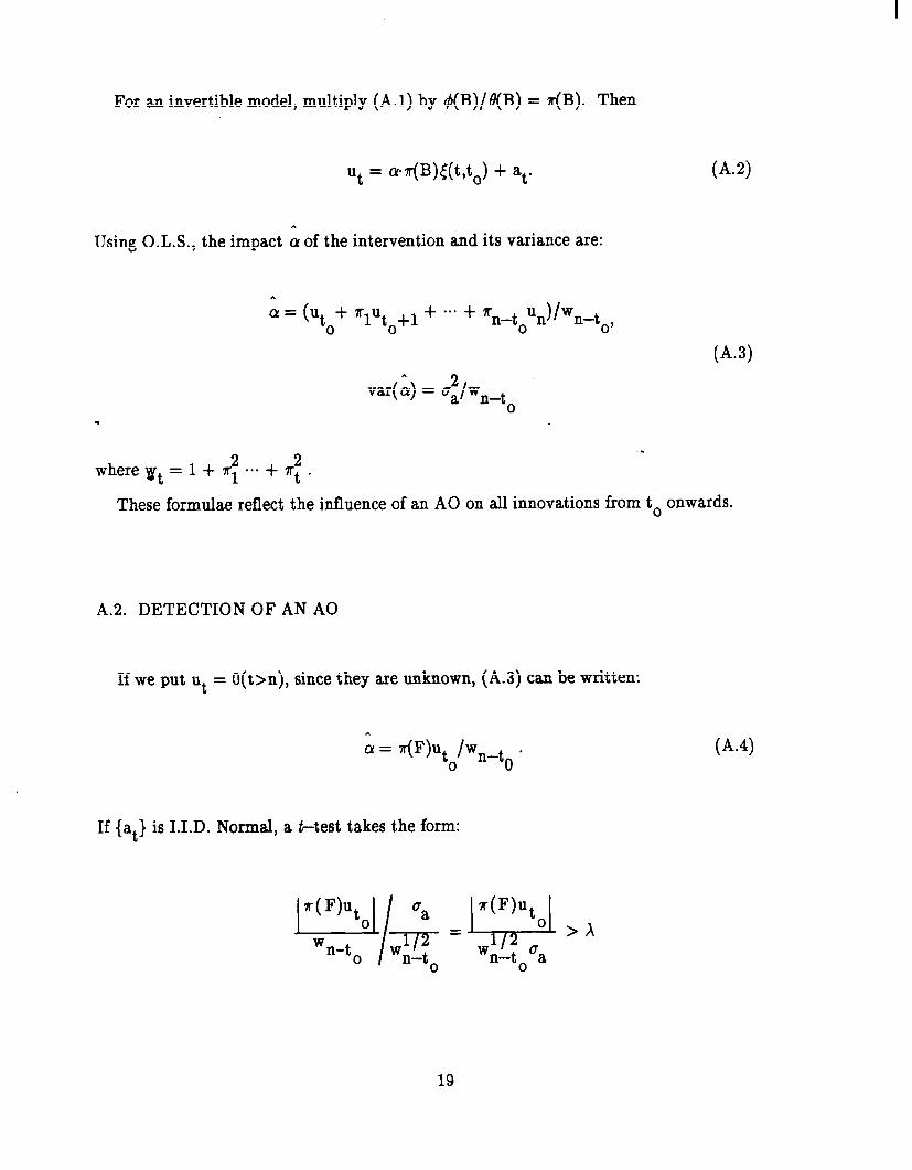
For an invertible model, multiply (A.l) by $(B)/e(B) = Ir(B). Then

Ut = m-(B)<(t,to) + at.

. Using O.L.S., the impact a! of the intervention and its variance are:

(A-2)

A = (Ut 0

+ “1Ut 0

+1 + -** + Q-t 0 Un)/Wn-t

0’

var( ;y> = ui/w,-t 0

.

.

where vt = 1 + r; *** + 7r; .

These formulae reflect the influence of an A0 on all innovations from to onwards.

A.2. DETECTION OF AN A0

If we put ut = O(t>n), since they are unknown, (A.3) can be written:

L * = tiFJUt lwnmt *

0 0

If {at} is I.I.D. Normal, a t-test takes the form:

(A.4

19

where A depends on the significance level. If to is unknown, and we define It = Ir(F) a

pass over the data is made to find those points where 1 It 1 > wnmt ‘j2Xaa. Note that w is a

function oft, so the test has a threshold that tapers downwards towards t=n.

The following developments arose from the first author’s discussion on the HBT paper

and subsequent collaboration with Dr. Bell. If t is not too near the start, ut = ‘Ir(B)zt so

It = e9~F)zt * (A4

This is a symmetric doubly-infinite moving average, in which missing values are replaced

by forecasts and backcasts. {I+,} behaves like the Irregular component in the traditional

decomcosition zt = Trend + Seasonal + Irregular.

In practice, when (n-t) exceeds about 2 years (depending on the model and parameters),

wn t closely approaches its final value wm. - By symmetry, the taper near the end of the

series is matched by a taper near the beginning: we cannot put ut = Ir(B) but instead

we use the model for the reversed series (which has the same ARMA parameters). If

vt = z(F)zt, then It = ‘K(B)vt, which will be valid, except near the end of the series. Thus

the test becomes: compute It = Ir(B)lr(F)zt, the first estimate of It. We define

wt = (wt if t<tL, wn - t if t>n-tL, We otherwise} and tL is the least t for which

wt > 0.95wm, (say), and a potential outlier is identified when:

1 it 1 > +2~ua . (A-6)

A.3. MULTIPLE AO’s

20

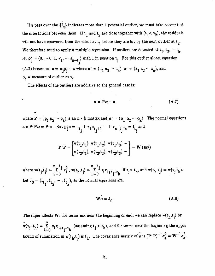
If a pass over the {It} indicates more than 1 potential outlier, we must take account of

the interactions between them. If tl and t2 are close together with (tl< t2), the residuals

will not have recovered from the effect at tl before they are hit by the next outlier at t2.

We therefore need to apply a multiple regression. If outliers are detected at tl, t2, ... tk,

let pj = (0, ..a 0, 1, ~1, a.. rn t ) with 1 in position tj. For this outlier alone, equation -.

(A.2) becomes: u = ~jpj + a wJhere u’ = (ul u2 ..’ un), a’ = (al a2 a.. a,), and

. = measure of outlier at aJ

t . . J

The effects of the outliers are additive so the general case is:

. u=Ptx+a - WV

.

where P = (PI P2 *-- %) is an n x k matrix and Q’ = (“1 Qi ... ok). The normaI equations

are P/Pa! = P/n. Butp;n= ut ad

j

+ T~u~+~ -.+ rnetun= It

j j ii

P’P = I w(tl’t1)’ “(tl’t& w(tpt3) ---

w(t2,tl)’ w(t2,t2), w(t2,t3) *-* 1 = w (say)

Il-tj 2 n-t. where w(tj,tj) = C

i=O pi , w(th,tj) = i ~oJ ~i~i+t .-t

= J h if tj> th, and W(th,tj) = W(‘j,th).

Let Jk = (It , It , .e. , It ), so the normal equations are: 1 2 k

Wi= Jo. (A4

The taper affects W: for terms not near the beginning or end, we can replace W(th,tj) by

w(tj-th) = ii 7r.T. i=O ’ l+tjIth

(assuming tj > th), and for terms near the beginning the upper

bound of summation in w(th,tj) is th’ The covariance matrix of A is (P) P)-‘ci = W-lo:,

21

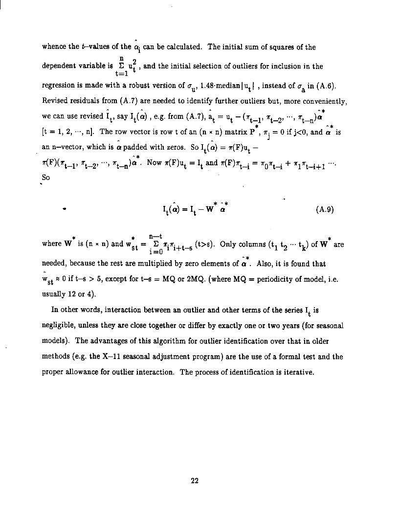
whence the &values of the 4 can be calculated. The initial sum of squares of the

dependent variable is i u2 t=1 t

, and the initial selection of outliers for inclusion in the

regression is made with a robust version of au, 1.48.median ] ut I , instead of aa in (A.6).

Revised residuals from (A.7) are needed to identify further outliers but, more conveniently,

we can use revised I,, say It(i) , e.g. from (A.7), at = ut - (ztsl, 7rtD2, ..., zt+)A*

[t = 1, 2, .“, n]. The row vector is row t of an (n x n) matrix P*, R. = 0 if j<O, and i* is

an n-vector, which is i padded with zeros. So It( & = a(F)ut - J

71F)(?rt_l, nt-2, . . . . ~t-n)h* Now Ir(F = It and “(F)“t-i = “o~tti + blot i+l . . . . -

so .

.

I&) = It - w* ;*

where W* is (n * n-t

x n) and w *

st = c T.-K. i-0 ’ l+ts

(t>a). ody column8 (tl t2 “’ tk) of W are

needed, because the rest are multiplied by zero elements of i*. Also, it is found that

wst x 0 if t-s > 5, except for t-s = MQ or 2MQ. (where MQ = periodicity of model, i.e.

usually 12 or 4).

In other words, interaction between an outlier and other terms of the series It is

negligible, unless they are close together or differ by exactly one or two years (for seasonal

models). The advantages of this algorithm for outlier identification over that in older

methods (e.g. the X-11 seasonal adjustment program) are the use of a formal test and the

proper allowance for outlier interaction. The process of identification is iterative.

22

REFERENCES

Barnett, V. and Lewis, T. (19781, Outliers in Statistical Data,

John Wiley & Sons: New York.

Bell, W. R. (19831, "A Computer Program (TEST) for Detecting

Outliers in Time Series," Proceedings of the American

Statistical Association Meetings, Chicago.

Bell, W. R. and Hillmer, S. C. (19841, "Issues involved with the

Seasonal Adjustment of Economic Time Series," Joumul of -

Buszfness 8 Bconomic Statistics, 2, 291-349.

Box, G.E.P., Hillmer, S. C., and Tiao, G. C. (19781, "Analysis

and Modeling of Seasonal Time Series," in Seasonal Analysis of

Economic Time Series, ed. A. Zellner, Washington, D. C.: U.S.

Department of Commerce, Bureau of the Census, 309-334.

Box, G.E.P. and Tiao, G. C. (1976). Intervention analysis with

applications to economic and environmental problems, Journal of

the American Statistical Association, 70, 70-79.

Burman, J. P. (19801, 'Seasonal Adjustment by Signal Extraction,"

Journal of the loyal Statistical Society, Ser. A, 143, 321-337.

(1983). Connnents on Modeling considerations in the

seasonal adjustment of economic time series in Applied Time

23

Series Analysis of Economic Data by Hillmer, Bell % Tiao (see

below).

Chronology of Recent Noteworthy Events (1962 to 19841, Monthly

memorandum for the Statistical Indicators Division of the

Bureau of Economic Analysis, Department of Commerce,

Washington, DC 20230. George R. Green, Acting Chief.

Denby, L. and Martin, R. D. (19791, "Robust Estimation of the

* First Order Autoregressive Parameter," Journal of- the American

Statistical Association, 74, 140-146. .

*

Draper, N., and Smith, H. (19841, Applied Regression Analysis,

Second Edition, John Wiley % Sons: New York.

Hillmer, S. C., Bell, W. R., and Tiao, G. C. (1983a), "Modeling

Considerations in the Seasonal Adjustment of Economic Time

Series," in Applied Time Series Analysis of Bconomic Data, ed.

A. Zellner, Washington, D-C.: U.S. Department of Comrmerce,

Bureau of the Census, 74-100.

(1983b) "Response to Discussants," in Applied Time Series

Analysis of Economic Data, ed. A. Zellner, Washington, D.C.:

U.S. Department of Cormnerce, Bureau of the Census, 123-124.

Shisken, J., Young, A-H., and Musgrave, J.C. (19671, "The X-11

Variant of the Census Method II Seasonal Adjustment Program,"

24

Technical Paper lo. 15, U.S. Dept. of Commerce, Bureau of

Economic Analysis.

.

.

L 25

List of Tables

GI'able 1. Outlier Study Series.

Table 2. ARIMA Models and Number of Outliers. .

Table:. Mean Forecasting Error, Seasonal Moving Average

Parameters, and Ljung-Box Statistics.

Table 4. Estimated Values of the Seasonal Moving-average

parameter (fl,,) for Chain Runs of Two Series.

Table 5. Effect of Outlier Modifications on the Mean Absolute

Forecast Error (MAFE) Ratios by Division.

Table 6. Effect of Changing Threshold from t=3 to t=2.5.

List of Figures

Figure 1. Forecasting Error Ratios vs. Number of Outliers. The

MAFE ratios are plotted against the number of outliers.

The horizontal reference line indicates no changes due

to outlier modification. Note, there is no correlation

between the percent change and how many outliers are

identified in the series.

Figure 2. Forecasting Error Ratios vs. Ljung-Box Ratios. The

MAFE ratios are plotted against the Ljung-Box Statistic *

ratios. The horizontal and vertical reference lines

indicate no change in the MAFE ratios and in the

Ljuug-Box ratios, respectively. Points in these upper

right quadrant indicate that not modifying for outliers

gives smaller forecasting errors and less

autocorrelation in the model residuals. Note, there is

no clear relation between the MAFE ratios and the model

statistics. The series with Ljung-Box statistics more

than doubled due to outlier modification is IGLCVS.

2

Figure 3. Forecast Error Ratios vs. Ratios of Mean Seasonal

Moving-average parameters. The MAFE ratios are

plotted against the mean of the t9,, estimates from the

chain run. The level of fi12 indicates the rate of

change in the seasonal pattern, values closer to one

being more stable. The vertical reference line

indicates no change in the stability of the seasonal

pattern due to outlier modification; points to the

right of this indicate that outlier modification

produces a more stable seasonal pattern. *Note that

there is no relation between the MAFE ratios and the *

change in the stability of the seasonal pattern due to

outlier modifications.

3

‘I

BVARRS s03000 533100 BWAPRS SO3000 560001

Construction Division BPlFAM

67-82 67-82

Retail sales of household appliances Total retail sales of automobiles Retail sales in department stores Retail sales of electrical goods Retail sales of furniture Wholesale sales of furniture Retail sales at gasoline stations Retail sales at grocery stores Wholesale sales at grocery stores Retail sales at hardware stores Wholesale sales at hardware stores Retail sales' at liquor stores Retail sales of men's clothes Retail sales of shoes Retail sales of sporting, recreational an photographic goods Retail sales at variety stores Retail sales of women's apparel

ClFTBP 64-83

C24TBP BP24FA 64-83

C5PTBP BP5PFA 64-83

CAOPVP PRAOTH 64-83

Total 1 family dwelling building permits Total 2 to 4 family duelling building permits Total 5+ family dwelling building permits Value in place, all other private residences

CNClBP XABPNClF 64-83

CNClHS XAHSNClF 64-83

CNC5HS XAHSNC5F 64-83

North Central 1 family building permits North Central 1 family housing starts North Central 5+ family housing starts

CNCTBP BPICRE 64-83 Total North Central building permits CNCTHS HSBC 64-83 Total North Central housing starts CNElBP XABPNElF 64-83 Northeast 1 family building permits CNElHS HSNElF 64-83 Northeast 1 family housing starts CNETBP BPNERE 64-83 Total Northeast building permits CNETHS HSNE 64-83 Total Northeast housing starts CSOTHS HSSO 64-83 Total South housing starts CWSTHS HSWT 64-83 Total West housing starts

TABLE 1, Outlier Studv Series

Series Division Code Years Description

Business Division BAPPRS SO3000 570002 BAUTRS s03000 550000 BDPTRS s03000 531100 BELGWS SO3000 506000 BFRNRS s03000 570001 BFRNWS SO3000 502000 BGASRS 503000 554100 -BGRCRS s03000 541100 BGRCWS s03000 514000 BHDWRS s03000 507000 @IDWWS SO3000 525100 BLCjRRS s03000 592100 BMNCRS SO3000 561100 BSHORS SO3000 566100 BSPGWS' s03000 504000

67-82 67-82 67-82 67-82 67-82 67-82 67-82 67-82 67-82 67-82 67-82 67-82 67-82 67-82 67-82

4

Series Division Code

Foreign Trade Division FCANXU XUCAN FCNCXU XUCARSC FEECXU XUEEC

FFPPXU XU058

FIRMXU xu2

FLARXU XULAR

FUNKXU XUUK

.FWGRXU XUWGER FWHMXU XUWH

Indus&v Division IBEVTI S62TI ICMETI N37TI

IFA'ITI S63TI IFMETI S23TI

IGLCTI S07TI

IHAPTI S35TI

ITVRTI S36TI

INEWUO S8OUO

ITVRUO S36UO

TABLE 1 (continued) Outlier Studv Series

Years Description

66-82 66-82 66-82

66-82

66-82

66-82

66-82

66-82 66-82

Unadjusted exports to Canada Unadjusted exports of cars to Canada Unadjusted exports to the European Ecomomic Community Unadjusted exports of fruits, preserves and produce Unadjusted exports of industrial raw materials Unadjusted exports to Latin American Republics Unadjusted exports to the United Kingdom Unadjusted e.xports to West Germany Unadjusted exports to the Western Hemisphere .

64-83 68-84

64-83 62-81

62-81

62-81

64-83

Total inventories of beverages Total inventories of communications equipment Total inventories of fats and oils Total inventories of farm machinery and equipment Total inventories of glass containers Total inventories of household appliances Total television and radio inventories

64-83 Unfilled newspaper, periodical, and magazine orders

64-83 Unfilled television and radio orders

IAPEVS

IBEWS ICMEVS

IFATVS IFMEVS

IFRTVS IGLCVS IHAPVS

IRREVS ITOBVS ITVRVS

N44VS

S62VS 64-83 N37VS 68-83

S63VS 62-81 S23VS 64-83

S86VS 62-81 so7vs 62-81 s35vs 64-83

S46VS 64-83 S65VS 64-83 S36VS 62-81

68-83 Value shipped of aircraft parts and equipment Value shipped of beverages Value shipped, communications equipment Value shipped of fats and oils Value shipped of farm machinery and equipment Value fertilizer shipped Value of glass containers shipped Value of household appliances shipped Value of railroad equipment shipped Value of tobacco shipped Value of televisions and radios shipped

.

6

Series Model

Business Division (O13>(Oll>12+TD+E, 8, = 0 BVARRS

BGRCRS

BHDWRS

BAPPRS

BWAPRS

BSHORS

BAUTRS

BFRNWS-

BSPGWS

BGASRS

BLQRRS

BMNCRS

BFRNRS

BDPTRS

BELGWS

BHDWWS

BGRCWS

(013)(011)12+TD+E, ti2 = 0

(o14)(oll)12+TD, 8, = 0

(olo>toll>12+TD

(012)(Oll)12+TD+E

(011) (011)12+TD+E

(110)(oll)12+TD

(oll>(oll>12+TD

(oll>(oll)12+TD

(011) (oll)12+TD

(012) (oll)12+TD

(101) (01q2+TD

(101) (olU12+TD

(101)(Oll)12+TD+E

(011) (olq2+TD

(oll>(oll>12+TD

(o13)(011)12+TD

TABLE 2. ARIMA Models and Number of Outliers

No. of Outliers Ext. Consistently

Totala Causes Identifiedb

.

7

aIdentified on at least one run. b Identified on all runs, but no cause houn.

8

Key: (000)12 = seasonal. means. TD = Trading Day adjustment. E = Easter

adjustment. "8' = 0" ARMA parameters that are less than their standard L

errors and are constrained to zero.

7

TABLE 2 (continued)

Series Model

Construction Division CAOPVP (310) (011) 12

CNClHS (200)(oll)12

CNC5HS (011>t011>,,

CNCTHS (101) (olq2

CNElHS (300) (011)12

CNETHS (101) (01q2

CSOTHS (100)(ooo)12

CNClBP (011)(011)12+TD

CNCTBR (100)(Oll)12+TD

CNElBP (210)(ooo)12

CNETBP (oll)(oll)12+TD

ClFTBP (011) (011)12+TD

C24TBP (oll)(oll)12+TD

No. of Outliers Ext. Consistently

Totala Causes Identifiedb

3

9

3

6

2

4

1

7

3

6

4

5

3

1

6

1

5

2

2

-1

5

3

5

4

1

2

1

1

3

7

1

C5PTBP

CWSTHS

(o13)(011)12, 02=o 3

(013>t011>,,

Foreign Trade Division FIRMXU (oll)(oll)12

39

1

FCANXU (011)(oll)12

FCNCXU (013) (oll)12 3

FWHMXU (011)(000>,, 6

FLARXU t013>t000>,2 7

FWGRXU (o11)(011)12 7

FUNKXU (011>t011>,, 5

FFPPXU t011>(011>,, 4

1

37

1

4

5

3

3

3

33

8

19 1

Series Model

Industrv Division ICMEVS (210) (011) 12

ICMETI

IGLCVS

IGLCTI

IFMEVS

IFMETI

IHAPTI

'ITVRVS

ITVRTI

IFATTf

IFATVS

ITOBVS

INEWVO

IAPEVS

IFRTVS

IHAPVS

IRREVS

IBEWS

IBEVTI

(310)(oll)12

(012>(011>12

(o13)(ooo)12

(019)(ooo)12 , B,=*. l =e8=o (210) (011) 12

(o12)(oll)12

(o12)(oll)12

(011>t011>,,

~014~~oll~12 , e2=e3=0

(011>(011>12

(013) (01q2

(011>t011),,

(011) (oll>l2

(011) (011)12

(011)(011)12

(o11)(011)12

(o14)(011)12+TD

(012) toll>,,

TABLE 2 (continued)

No.

Totala

5

3

9

4

5

10

3

1

2

6

2

11

2

3

5

71

aIdentified on at least one run. b Identified on all runs, but no cause tioun.

of Outliers Ext. Consistently

Causes

3

7

3

4

7

1

1

2

2

4

34

Identifiedb

2

3

1

1

1 .

1

5

2

2

Key: (000)12 = seasonal means. TD = Trading Day adjustment. E = Easter

adjustment. 11 ei = 0" ARMA parameters that are less than their standard

errors and are constrained to zero.

9

Z'PE L'EE L'9P 8EO' 990' 5X0' 169' 289' 099' 8ZS;T' 6TF;T' !iL!ii l

O'!X O'!X 9'TZ !iZO' 6ZO' LZO' 99L' TOL' ETL' 2822' 8EZZ' OLZZ' 0'I;T L'9T 8'9T LTO' ZZO' 610' EEL' Z&L' ZLL' s;LGZ' !xEE - 9PPE - L'EZ Z'9T E'OE PEO' E90' !xo- T6L' 008' OEL' 1991. E88T' OTTZ'

(,)ZL80' L980'

P'LZ Z'6Z E'EZ PTO' 600' 600' 826' P68' L68' 0990 - 6L90' I;L90'

O'EE E'OE: 2'82 9ZO' EEO' EZO' PE9' 'iP9' 089'

E’EZ 8'PZ T'PZ ZPO' E90' LPO' PEL' 91;L' 99L' L'PP P'LP 9'!x szo* 9ZO' 9ZO' L6L' ZSL' ZT8' E'LZ T'SZ 0'9Z LTO' 9TO' ZTO' L89' 669' OZL' L'OP P'OP Z'!X LOO' LOO' 800' 6P9' 8P9' TP9' 9'9Z 9'LZ O'OE 610' STO' ETO' SOL' L89' 8EL' L'PT O'!x 9.91 LTO' EZO' HO' 8%' Z9E' ZEP' P-T& O'OE 0-W 8PO' HO' 6PO' 168' 8L8' Z28'

L'PE T'ZE 8'ZP ZTO' 610' &TO' 1;9t- SZL' EPL'

TL90' TS90' 9990 - (,)&LPO' P6PO'

09PO - E9PO - P8PO' OL90' 6990' POLO - 8LEO' LLEO' 6LEO' 9ZEO - 9zco l 9ZEO -

6OPO' 8OPO' TWO' 9ZEO' OPEO - O!xO - 9600' L600' 6600'

OS OH n OS OH II OS OH ’ a OS OH n (s-3 PZ)

b xoa-gun [I tZTe)as tZTe) U=H 3dVI

SHTBNil SHJ3N3 SH93N3 SHT3N3

(sun1 9)

dAdOV3

SAN168 sImv8 snoHs8 SndVAa SlddVa snhaHa swaa

mm8

sapas

. .

. .

. .

. .

. .

. .

. .

. .

. 00

00

0 h

)o

wo

o

+w

C

LCLC

I w

C

L o

oa

lcn

w

Q,

No

0 C

nr0

-l 00

c

p-

h3w

w

oh

3 V

II&r

+

-J

000

cn

w

oo

cn

o

-4o

a

cn

hb

-lta

w

C

ntP

+

ww

w

w

wm

qw

q

-

. .

. .

. .

.

w

. .

. .

. .

. -a

oo

wo

w

sa

w

mo

o00

w

o

ote

Q

soo

oo

t4

w

*

. .

. .

. .

. .

. .

. .

. .

-ao

ow

w

w

saw

o

oo

ow

c

ow

-3

-a

t3c

no

oc

n

w

oo

ta

ow

l-b

OQ

, c

nw

o

oc

n-lo

c

n

-a0

CIo

Icn

C

QW

W

C0

. .

. .

. .

. o

sww

w

w

oa

w

-ab

bl.b

tP

w

oa

r -lr

tao

c

o

0000

. .

. .

I .*

oo

oi

i 00

C

L++

h

hW

Icl

ror

a

ch

ta-3

--

. .

. I

0001

I

bb

o

oh

3 h

h

CLW

w

wo

l-h

*-

a00

-v

. .

. .

. .

. -lw

w

ww

-J

Joo

W

-JLG

00

7 o

oh

) N

rpc

p

raJ

ow

L-61 8'ZZ L-PI P'PZ 9'ZZ 9'EZ

9'OZ 8'ZZ T'ZZ 6'ST L-91 E'!iP 9'PE: Z'SE T'8E 9'82 T'TE 6*&E 8'TE 9'6Z E'ZZ L'EZ L'PZ 9'EZ S'SZ 8'OE S'OZ T-ET Z-ET L'9Z 8'OP S'TP Z'LE: S'9Z 6'82 O'EZ T'8Z T'9Z 6'6 8'1;Z 8'PZ E'ZZ S'EZ 9'LZ E'LT

PPO' 280' 9EO' Z&O' 9PO' (3)-- STO' 8TO' PZO' PTO' 910' HO' LZO' 920' 610' OZO' 9PO' 9PO' LOO‘ LOO' 900' ZZO' LZO' EZO' EZO' OEO' EZO' TTO' EPO' STO'

(P)-- (P)-- (P)-- w- w- (P)-- OTO’ ZTO’ 600' PZO' PEO' SZO' 8TO' 9TO' 6TO'

8PE' SSE' TIP' T98' 6P8' EL6'

089' EL9' E61;' LTL' ZTL' 6PL' t8L' L8L' LEL' E69' 8P9' LP9' 9T8' TZ8' ZZ8' ZP9' LE9' LP9' OP8' 8P8' LP8' 91;L' C9L' 908' 000-T OOO'T OOO'T

8P6' 096' 000-T 9&8 - 9P8' LL8' TOL' E89' P69: 6TL' L89' '26L'

(,)S980' EZ80' (sunl TT)

LP80' . 8LLO'

96PO' TLSO' OTLO' Ki80' TLEO' T90T l TPZO�

szzo -

ET60'

'ZCZO'

SPPO - LLOO' SZEO'

-8060' Z&80'

99so l

9s90 l

6TLO' 6P80' OLEO' 6901 l

OPZO l

sozo l

1160'

6ZZO'

9SPO - 6LOO' SZEO -

OS OH n n OS OH n OS. OH

am b

(s-3 PZ) xofl-9un [I

OS (ZTeD;as (ZTe> u=H

‘(SlOJJ3 ~sx!clalod a%nIosqv UoaH) 3dvH

(paw wo3) c 37avz

P980 l

OPLO'

TLSO' PL90' 8TLO' 9S80' PLEO' 1901. TZZO' zozo - X60'

TZZO�

OSPO �

8LOO' 9PEO l

n

SAJJadI SA3dVI OfMaN SAaOJJ SAJVdI ILlJdI IJl’tlAJJ SA’IIAJI I,T,dVHI IiCBIdI SA3RIdI IiIJ’I31 SA3131 IJBI31 SABWDI

sarIaS

.-

TABLE 4

Estimated e12 on Unadjusted (U), Modified Series (MO) end

Simultaneously Estimated Outliers (SO) Runs

CNClHS ICMEVS Run No. U MO so U MO so

*

1 .704 ,820 2 .713 .827 3 .720 .842 4 .746 .853 5 .731 .827 6 .667 .711 7 .656 .710 8 .666 .737 9 ,686 -750 10 .786 .842 11 .810 .835 12 ,809 -834

13 ,791 -815

.796

.780

.794

.808 ,801 .748 .737 ,747 .762 .827 .835 ,836

a ----

.794 .667 ,774 .668 .771 -664 .784 .680 ,775 .672 .786 .684 .797 ,697 .818 .706 .807 .693 .798 ,691 .798 .697 ,794 ,701

,839 ,715

.696

.697‘

.694

.712

.703

.717

.731

.742

.735

.730 ,733 .733

a em--

Note: The estimated model of the first run for each series uses data with the last three years removed, the 12th run only has three months revved, and the last, 13th ruu, is on the full data. The three columns for each series are U = unadjusted series, MO = modified series, and SO = outliers simultaneously estimated in model.

au-A. because the 13 th

SO run was made purely to provide "actuals" for comparison with the post-sample forecasts, and the former were modified for glJ identified outliers.

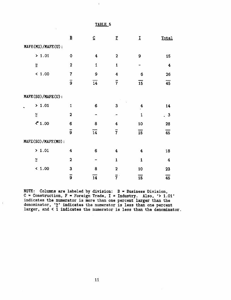
TABLE 5

MAFE(MO)/MAFE(U):

> 1.01

N =

c 1.00

MAFE(SO)/MAFE(U):

. > 1.01

N =

Cl.00

B c

0 4

2 1

7 9

9 ii

1 6

2

6 8

9 ii

MAFE(SO)/MAFE(MO):

> 1.01 4 6

N = 2

< 1.00 3 8

9 ii

2 9

1

4 6

'7 15

3 4

1

4 10

7 ii

4 4

1 1

2 10 -. 7 15

Total

15

4

26

45

14

-3

28

45

18

4

23

45

NOTE : Columns are labeled by division: B = Business Division, C = Construction, F = Foreign Trade, I = Industry. Also, '> 1.01' indicates the numerator is more than one percent larger than the denominator, 'g' indicates the numerator is less than one percent larger, and < 1 indicates the numerator is less than the denominator.

11

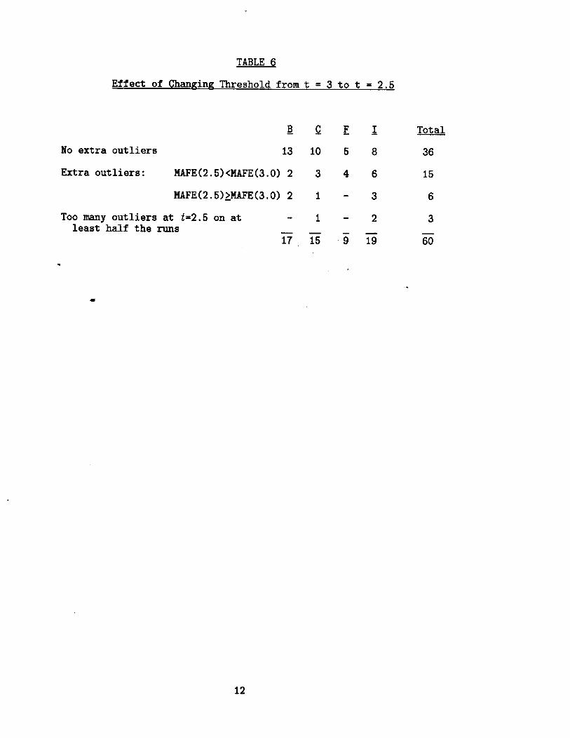
TABLE 6

Effect of Channinn Threshold from t = 3 to t = 2.5

B c No extra outliers 13 10

Extra outliers: MAFE(2.5)CMAFE(3.0) 2 3

MAFE(2.5),MAFE(3.0) 2 1

Too many outliers at t=2.5 on at 1 least half the X-UTH

i7 15

.

E L Total

5 8 36

4 6 15

3 6

2 3

ii iii so

.

12

.

0.7

0.8

MA

FE(S

0)

,’ M

AFE

(U)

0.9

1.0

1.1

1.2

1.3

MA

FE(S

0)

/ M

AFE

(U)

0.7

0.8

0.9

1.0

1.1

1.2

1.3

X

y+

in

>

2 X

I X

X)

w--

3i

x >;

2s

5

WI

0 x

x w

x

x

\z-

>

r-

-. c

X

X

x”

MA

FE(S

0)

/ M

AFE

(U)

0.7

0.8

0.9

1.0

1.1

1.2

1.3

0

-I

T CD

E;-

c

X