time series outlier detection - ucsd mathematicst8zhu/talks/ts outlier detection.pdfoutline time...

Time Series Outlier Detection

Tingyi Zhu

July 28, 2016

Tingyi Zhu Time Series Outlier Detection July 28, 2016 1 / 42

Outline

Time Series Basics

Outliers Detection in Single Time Series

Outlier Series Detection from Multiple Time Series

Demos


Time Series Basics


First-order Autoregression

A model denoted as AR(1), in which the value of X at time t is a linearfunction of the value of X at time t − 1:

Xt = φXt−1 + εt (1)

Assumptions:

εti .i .d∼ N(0, σ), stochastic term.

εt is independent of Xt .


General Autoregressive ModelAR(p):

Xt = φ1Xt−1 + φ2Xt−2 + · · ·+ φpXt−p + εt

=

p∑i=1

φiXt−i + εt

=

p∑i=1

φiBiXt + εt

where we use the backshift operator B (BXt = Xt−1, BkXt = Xt−k).

Alternative notation:φ(B)Xt = εt

φ(B) is a polynomial of B,

φ(B) = 1− φ1B − φ2B2 − · · · − φpBp = 1−p∑

i=1

φiBi


Moving Average

Another approach for modeling univariate time series

Xt depends linearly on its own current and previous stochastic terms

MA(1):

Xt = εt + θ1εt−1

MA(q):

Xt = εt + θ1εt−1 + · · ·+ θqεt−q


θ1, . . . , θq: parameters of MA model

εt , . . . , εt−q: stochastic terms

Using backshift operator B, model simplified as

Xt = (1 + θ1B + · · ·+ θqBq)εt

= (1 +

q∑i=1

θiBi )εt

= θ(B)εt


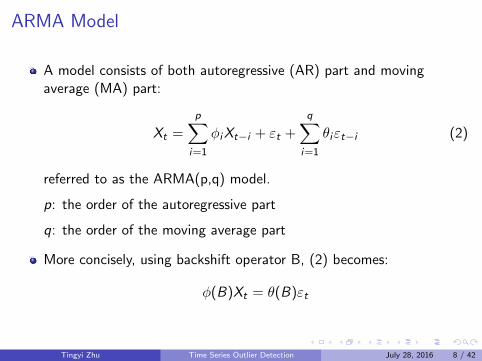
ARMA Model

A model consists of both autoregressive (AR) part and movingaverage (MA) part:

Xt =

p∑i=1

φiXt−i + εt +

q∑i=1

θiεt−i (2)

referred to as the ARMA(p,q) model.

p: the order of the autoregressive part

q: the order of the moving average part

More concisely, using backshift operator B, (2) becomes:

φ(B)Xt = θ(B)εt


Stationarity of Time Series

In short, a time series is stationary if its statistical properties are allconstant over time.

To mention some properties:

Mean: E [Xt ] = E [Xs ] for any t, s ∈ Z ,

Variance: Var [Xt ] = Var [Xs ] for any t, s ∈ Z ,

Joint distribution:

Cov(Xt ,Xt+1) = Cov(Xs ,Xs+1) for any t, s ∈ Z.


Requirements for a Stationary Time Series

AR(1) Xt = φXt−1 + εt : |φ| < 1

AR(p) φ(B)Xt = εt :

All the roots of φ(z) = 0 are outside unit circle.

MA models are always stationary

ARMA(p,q) φ(B)Xt = θ(B)εt :

All the roots of φ(z) = 0 are outside unit circle.


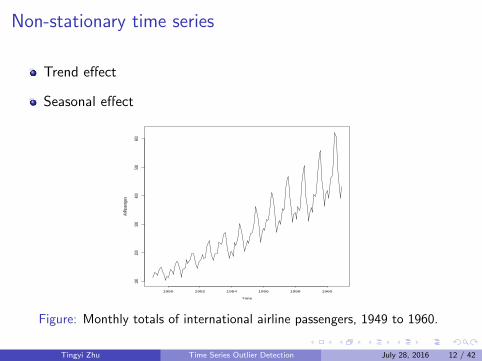
Non-stationary time series

Trend effect

Seasonal effect

Time

AirPa

ssen

gers

1950 1952 1954 1956 1958 1960

100

200

300

400

500

600

Figure: Monthly totals of international airline passengers, 1949 to 1960.


Time Series Decomposition

Think of a more general time series formulation including both trendand seasonal effect:

Xt = Tt + St + Et (3)

I Xt is data point at time t

I Tt is the trend component at time t

I St is the seasonal component at time t

I Et is the remainder component at time t (containing AR and MAterms)


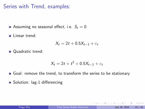
Series with Trend, examples:

Assuming no seasonal effect, i.e. St = 0

Linear trend:

Xt = 2t + 0.5Xt−1 + εt

Quadratic trend:

Xt = 2t + t2 + 0.5Xt−1 + εt

Goal: remove the trend, to transform the series to be stationary

Solution: lag-1 differencing


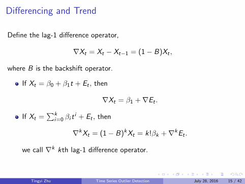
Differencing and Trend

Define the lag-1 difference operator,

∇Xt = Xt − Xt−1 = (1− B)Xt ,

where B is the backshift operator.

If Xt = β0 + β1t + Et , then

∇Xt = β1 +∇Et .

If Xt =∑k

i=0 βi ti + Et , then

∇kXt = (1− B)kXt = k!βk +∇kEt .

we call ∇k kth lag-1 difference operator.


Lag-1 Differencing

Jan 04

2016

Mar 01

2016

May 02

2016

Jul 01

2016

18

50

19

50

20

50

21

50

S&P 500 Quote Year−To−Date

Jan 04

2016

Mar 01

2016

May 02

2016

Jul 01

2016

−8

0−

60

−4

0−

20

02

04

0

S&P 500 YTD Lag−1 Differencing


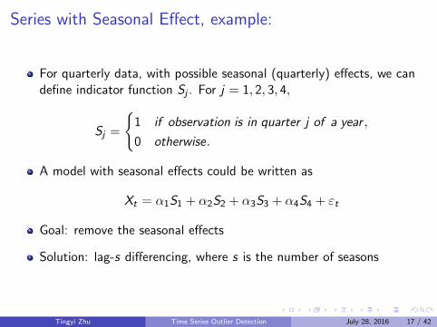
Series with Seasonal Effect, example:

For quarterly data, with possible seasonal (quarterly) effects, we candefine indicator function Sj . For j = 1, 2, 3, 4,

Sj =

{1 if observation is in quarter j of a year ,

0 otherwise.

A model with seasonal effects could be written as

Xt = α1S1 + α2S2 + α3S3 + α4S4 + εt

Goal: remove the seasonal effects

Solution: lag-s differencing, where s is the number of seasons


Differencing and Seasonal Effects

Define the lag-s difference operator,

∇sXt = Xt − Xt−s = (1− Bs)Xt ,

where B is the backshift operator.

If Xt = Tt + St + Et , and St has period s (i.e. St = St−s for all t), then

∇sXt = (1− Bs)Xt = Tt − Tt−s +∇sEt .


Non-seasonal ARIMA

St = 0

ARIMA stands for Auto-Regressive Integrated Moving Average,ARMA integrated with differencing.

A nonseasonal ARIMA model is classified as ARIMA(p,d,q), where

I p is the order of AR terms,

I d is the number of nonseasonal differences needed for stationarity,

I q is the order of MA terms.


Non-seasonal ARIMA, Cont.

Recall ARMA(p,q):

φ(B)Xt = θ(B)εt ,

I φ(B) and θ(B) are polynomials of B of order p and q.

I Stationary requirement: all roots of φ(z) = 0 outside unit circle.

ARIMA(p,d,q):

φ(B)(1− B)dXt = θ(B)εt ,

I Xt is not stationary. Why?

I Zt = (1− B)dXt is ARMA(p,q), is stationary.


Seasonal ARIMA

A seasonal ARIMA model is classified as

ARIMA(p, d , q)× (P,D,Q)m

I p is the order of AR terms,

I d is the number of nonseasonal differences,

I q is the order of MA terms.

I P is the order of seasonal AR terms,

I D is the number of seasonal differences,

I Q is the order of seasonal MA terms.

I m is the number of seasons.


Example: ARIMA(1, 1, 1)× (1, 1, 1)4


General ARIMA

The ARIMA model can be generalized as follow:

φ(B)α(B)Xt = θ(B)εt ,

I φ(B): autoregressive polynomial, all roots outside unit circle

I α(B): differencing filter renders the data stationary, all roots on theunit circle

I θ(B): moving average polynomial, all roots outside unit circle (toassure θ(B) is invertible.

Alternatively,

Xt =θ(B)

φ(B)α(B)εt .


Outliers Detection in Single Time Series


Automatic Detection Procedure

Described in Chung Chen, Lon-Mu Liu. Joint Estimation of ModelParameters and Outlier Effects in Time Series,JASA, 1993

Based on the framework of ARIMA models

R package tsoutlier written by YAHOO in 2014


Types of Outliers

General representation: L(B)It(tj)

I L(B): a polynomial of lag operator B

I It(tj) = 1 there’s outlier at time t = tj , and 0 otherwise.

Types of outliers:

I Additive Outliers (AO): L(B) = 1;

I Level Shift (LS): L(B) = 11−B ;

I Temporary Change (TC): L(B) = 11−δB ;

I Seasonal Level Shift (SLS): L(B) = 11−Bs ;

I Innovational Outliers (IO): L(B) = θ(B)φ(B)α(B) .


Types of Outliers


Formulation

ARIMA model:

Xt =θ(B)

φ(B)α(B)εt .

Model with outliers at time t1, t2, . . . , tm:

X ∗t =

m∑j=1

ωjLj(B)It(tj) +θ(B)

φ(B)α(B)εt .

I Lj(B) depends on pattern of the jth outlier

I It(tj) = 1 there’s outlier at time t = tj , and 0 otherwise.

I ωj denotes the magnitude of the jth outlier effect


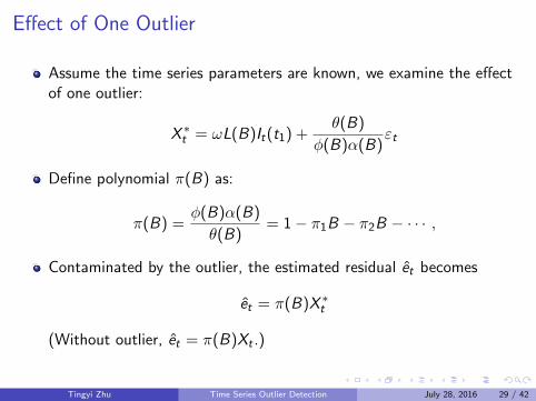
Effect of One Outlier

Assume the time series parameters are known, we examine the effectof one outlier:

X ∗t = ωL(B)It(t1) +

θ(B)

φ(B)α(B)εt

Define polynomial π(B) as:

π(B) =φ(B)α(B)

θ(B)= 1− π1B − π2B − · · · ,

Contaminated by the outlier, the estimated residual et becomes

et = π(B)X ∗t

(Without outlier, et = π(B)Xt .)


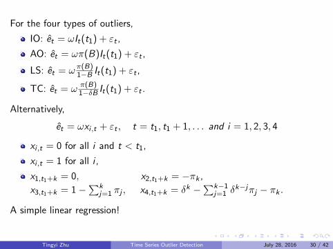
For the four types of outliers,

IO: et = ωIt(t1) + εt ,

AO: et = ωπ(B)It(t1) + εt ,

LS: et = ω π(B)1−B It(t1) + εt ,

TC: et = ω π(B)1−δB It(t1) + εt .

Alternatively,

et = ωxi ,t + εt , t = t1, t1 + 1, . . . and i = 1, 2, 3, 4

xi ,t = 0 for all i and t < t1,

xi ,t = 1 for all i ,

x1,t1+k = 0, x2,t1+k = −πk ,

x3,t1+k = 1−∑k

j=1 πj , x4,t1+k = δk −∑k−1

j=1 δk−jπj − πk .

A simple linear regression!


Estimate of ω

The least square estimate doe the effect of a single outlier at t = t1 canbe expressed as


Test Statistics τ

From regression analysis, we have

ω − ωσa

(n∑

t=t1

x2i ,t)1/2 ∼ N(0, 1),

where σa is the estimation of residual standard deviation.

We want to test whether ω = 0 , then the following statistics areapproximately N(0, 1):


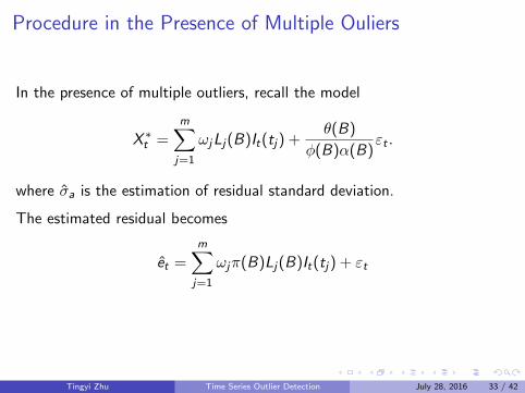
Procedure in the Presence of Multiple Ouliers

In the presence of multiple outliers, recall the model

X ∗t =

m∑j=1

ωjLj(B)It(tj) +θ(B)

φ(B)α(B)εt .

where σa is the estimation of residual standard deviation.

The estimated residual becomes

et =m∑j=1

ωjπ(B)Lj(B)It(tj) + εt


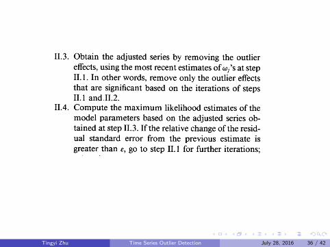
Stage 1: Joint Estimation of Outlier Effect and ModelParameters

Fitting the series by an ARIMA model (forecast package in R),obtain initial parameter (φ(B), θ(B), α(B)) estimation of the model.

Detect outliers one by one sequentially


Stage 2: Initial Parameter Estimation and OutlierDetection


Outlier Series Detection from Multiple Time Series


Detect Anomalous Series

Goal: efficiently find the least similar time series in a large set

Motivation: Internet companies monitoring the servers(CPU,Memory), find unusual behaviors


Detect Anomalous Series

Described in Rob J Hyndman et al. Large-Scale Unusual Time SeriesDetection, ICDM, 2015

Approach: Extract features from time series, PCA

R package anomalous

Test on real data from YAHOO email server,80% accuracy compared to 40% from previous methods


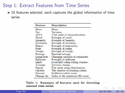
Step 1: Extract Features from Time Series

15 features selected, each captures the global information of timeseries


Step2: PCA to reduce dimension

I dim=15 initially, correlation existing between features

I The first 2 PCs are sufficient, capturing most of the variance

Step 3: Implement multi-dimentional outlier detection algorithm tofind outlier series

I Density based

I α-hull


Demo


time series outlier detection - ucsd mathematicst8zhu/talks/ts outlier detection.pdfoutline time...

Documents