quality assurance using outlier detection for …

QUALITY ASSURANCE USING OUTLIER DETECTION FOR AUTOMATIC SEGMENTATION OF CEREBELLAR

PEDUNCLES

by

Ke Li

A thesis submitted to Johns Hopkins University in conformity with the requirements for the degree of Master of Science in Engineering

Baltimore, Maryland

August, 2015

© 2015 Ke Li All Rights Reserved

ii

Abstract

Cerebellar peduncles (CPs) are white matter tracts that connect the cerebellum to

other brain regions. Automatic segmentation and quantification methods of the CPs are

important for objectively and efficiently studying their structure and function. Usually the

performance of automatic segmentation methods is evaluated by comparing with manual

delineations (ground truth). However, while this approach characterizes the performance

in an average sense, when a segmentation method is run on new data (for which no

ground truth exists) it is highly desirable to be able to efficiently detect and assess

algorithm failures so that these cases can be excluded from scientific analysis or rerun

with different parameters.

This thesis focuses on better understanding the performance of an automatic CP

segmentation method using two kinds of outlier detection methods. One is a simple

univariate non-parametric method using box-whisker plots. The other is a supervised

classification method. The content of this thesis is divided into three parts. First, a new

segmentation pipeline and its validation are described. The validation is performed by

two statistical tests with respect to two segmentation quality metrics. Results show that

segmentation labels from the new pipeline are statistically the same as those from the old

pipelines and the new pipeline performs even better on segmenting the decussation of the

superior cerebellar peduncles (dSCPs).

In the second part of this thesis, the univariate outlier detection method using box-

whisker plots is described. Automatic segmentation labels of a dataset with 48 subjects

iii

were manually categorized as successful segmentations or segmentation failures. Three

kinds of features were extracted from the categorized failures and then used for failure

detection. Performances of these features were quantitatively compared.

In the third part of this thesis, both box-whisker plots and the supervised

classification method applied to two datasets with a total of 249 manually categorized (as

success or failure) automatic segmentation labels are described. Four classifiers—linear

discriminant analysis (LDA), logistic regression (LR), support vector machine (SVM),

and random forest classifier (RFC) were used for failure detection. Each classifier’s

performance was evaluated using a leave-one-out cross-validation. Results show that the

performances among the LDA, SVM and RFC are not very different and LR performs

worse than the other three classifiers.

This thesis is prepared under the direction of Dr. Jerry L. Prince. The other two

readers are Dr. Bruno M. Jedynak and Dr. Sarah H. Ying.

iv

Acknowledgements

I would like to express my sincere appreciation to my research advisor, Dr. Jerry

L. Prince, for his guidance, consistent encouragement and support, and many useful

discussions during this research project. I really appreciate that Dr. Prince spent a lot of

time on reviewing and correcting my thesis. I would also like to thank Dr. Bruno M.

Jedynak for his suggestion of how to identify outliers easily and Dr. Sarah H. Ying for

her helpful comments on revising my thesis. Furthermore, I would like to thank the

members of the Image Analysis and Communications Lab for their kind help in the

research, particularly Zhen Yang, Dr. Chuyang Ye, Jeff Glaister, Amod Jog, Aaron

Carass, and Dr. Min Chen. Last, I want to thank my family and friends for their support

and encouragement.

v

Table of Contents

Abstract .............................................................................................................................. ii

Table of Contents .............................................................................................................. v

List of Tables ................................................................................................................... vii

List of Figures ................................................................................................................... ix

Chapter 1 Introduction ..................................................................................................... 1

1.1 Thesis Contributions ................................................................................................................ 5

1.2 Thesis Organization .................................................................................................................. 6

Chapter 2 Background ..................................................................................................... 9

2.1 Automatic Segmentation Method of Cerebellar Peduncles ............................................. 9

2.2 Quality Assurance in Medical Imaging Field .................................................................. 12

2.3 Outlier Detection Methodologies ........................................................................................ 15

Chapter 3 Validation of the New Algorithm Pipeline .................................................. 20

3.1 Algorithm Pipelines ............................................................................................................... 21

3.1.1 CATNAP ........................................................................................................................................... 21

3.1.2 The segmentation pipelines ......................................................................................................... 21

3.2 Comparison of Segmentation labels ................................................................................... 25

3.2.1 Description of the Tomacco dataset .......................................................................................... 25

3.2.2 Comparison results ......................................................................................................................... 26

3.3 Statistical Tests ....................................................................................................................... 29

vi

3.3.1 Tests on the Dice coefficients ..................................................................................................... 29

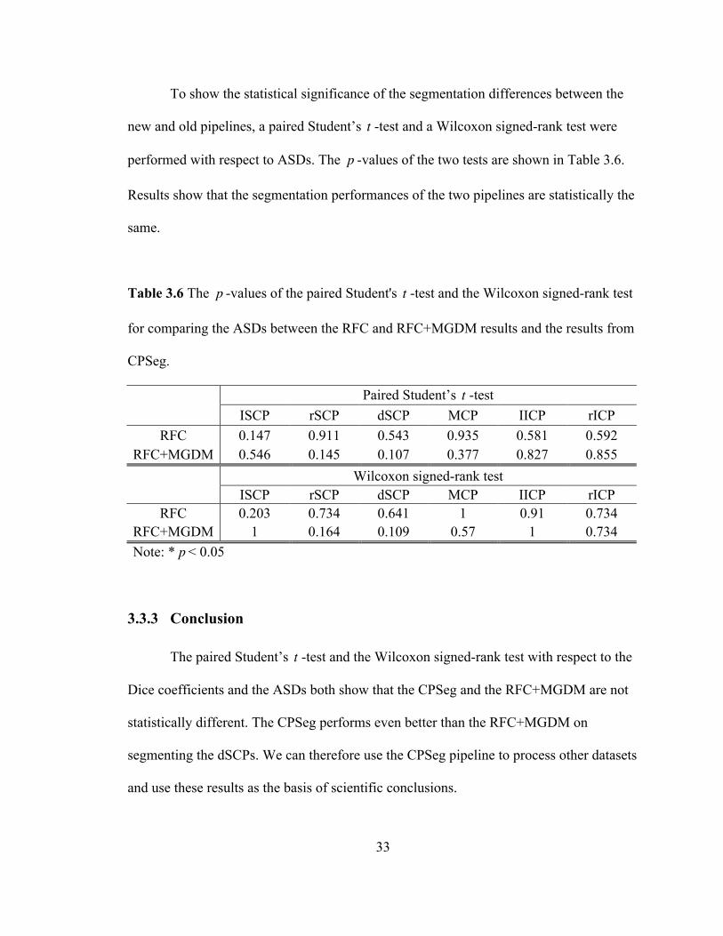
3.3.2 Tests on the average surface distances (ASDs) ..................................................................... 32

3.3.3 Conclusion ......................................................................................................................................... 33

Chapter 4 Outlier Detection on the Tomacco Dataset ................................................. 34

4.1 Categorization of Automatic Segmentations .................................................................... 34

4.2 Feature Extraction ................................................................................................................. 38

4.3 Outlier Detection Results ..................................................................................................... 43

Chapter 5 Outlier Detection on the Kwyjibo and Tomacco Datasets ........................ 50

5.1 Categorization of Automatic Segmentations .................................................................... 52

5.2 Outlier Detection Results ..................................................................................................... 56

5.3 Verification of the CATNAP-v2 Algorithm ..................................................................... 63

5.4 Reproduction of the Tomacco Dataset .............................................................................. 67

5.5 Outlier Detection using Classification Methods .............................................................. 74

5.5.1 The four classifiers ......................................................................................................................... 74

5.5.2 Training sets ...................................................................................................................................... 75

5.5.3 Performance evaluation ................................................................................................................. 76

Chapter 6 Conclusions and Future Work .................................................................... 79

6.1 Main Contributions ............................................................................................................... 79

6.2 Future Work ........................................................................................................................... 81

Bibliography .................................................................................................................... 83

Vita ................................................................................................................................... 89

vii

List of Tables

Table 3.1 The Dice coefficients between the manual delineations and the segmentation

labels in the two RFC processes in the RFC+MGDM and CPSeg pipelines,

respectively. .............................................................................................................. 30

Table 3.2 The Dice coefficients between the manual delineations and the final

segmentation labels in the two MGDM processes in the RFC+MGDM and CPSeg

pipelines, respectively. .............................................................................................. 30

Table 3.3 The p -values of the paired Student's t -test and the Wilcoxon signed-rank test

for comparing the Dice coefficients between the RFC and RFC+MGDM results and

the results from CPSeg. ............................................................................................. 31

Table 3.4 The ASDs between the manual delineations and the segmentation labels in the

two RFC processes in the RFC+MGDM and CPSeg pipelines, respectively. .......... 32

Table 3.5 The ASDs between the manual delineations and the final segmentation labels

in the two MGDM processes in the RFC+MGDM and CPSeg pipelines,

respectively. .............................................................................................................. 32


for comparing the ASDs between the RFC and RFC+MGDM results and the results

from CPSeg. .............................................................................................................. 33

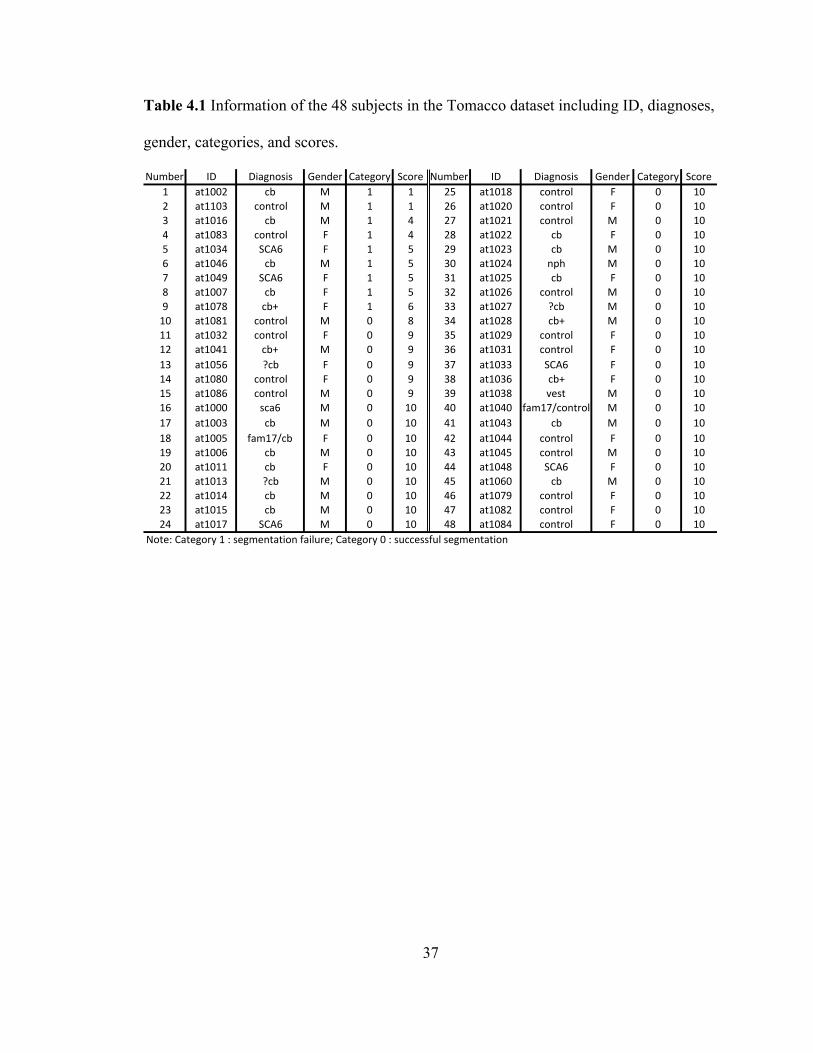
Table 4.1 Information of the 48 subjects in the Tomacco dataset including ID, diagnoses,

gender, categories, and scores. .................................................................................. 37

Table 4.2 Outlier detection results by selected features of the Tomacco dataset. The top

viii

nine subjects were manually categorized as segmentation failures in this dataset. .. 49

Table 5.1 Information of the categorized segmentation failures and imperfect but

successful segmentations in the Kwyjibo dataset including ID, diagnoses, gender,

categories, and scores. ............................................................................................... 54

Table 5.2 Outlier detection results by selected features on the Kwyjibo dataset. The top

eight subjects were manually categorized as segmentation failures in this dataset. . 62


gender, categories, and scores. .................................................................................. 68

Table 5.4 Outlier detection results by selected features of the reprocessed Tomacco

dataset. Four subjects were manually categorized as segmentation failures in this

dataset. ...................................................................................................................... 73

Table 5.5 Performance comparison of the four classifiers (LDA, LR, SVM, and RFC) on

the combined Tomacco and Kwyjibo dataset. .......................................................... 78

ix

List of Figures

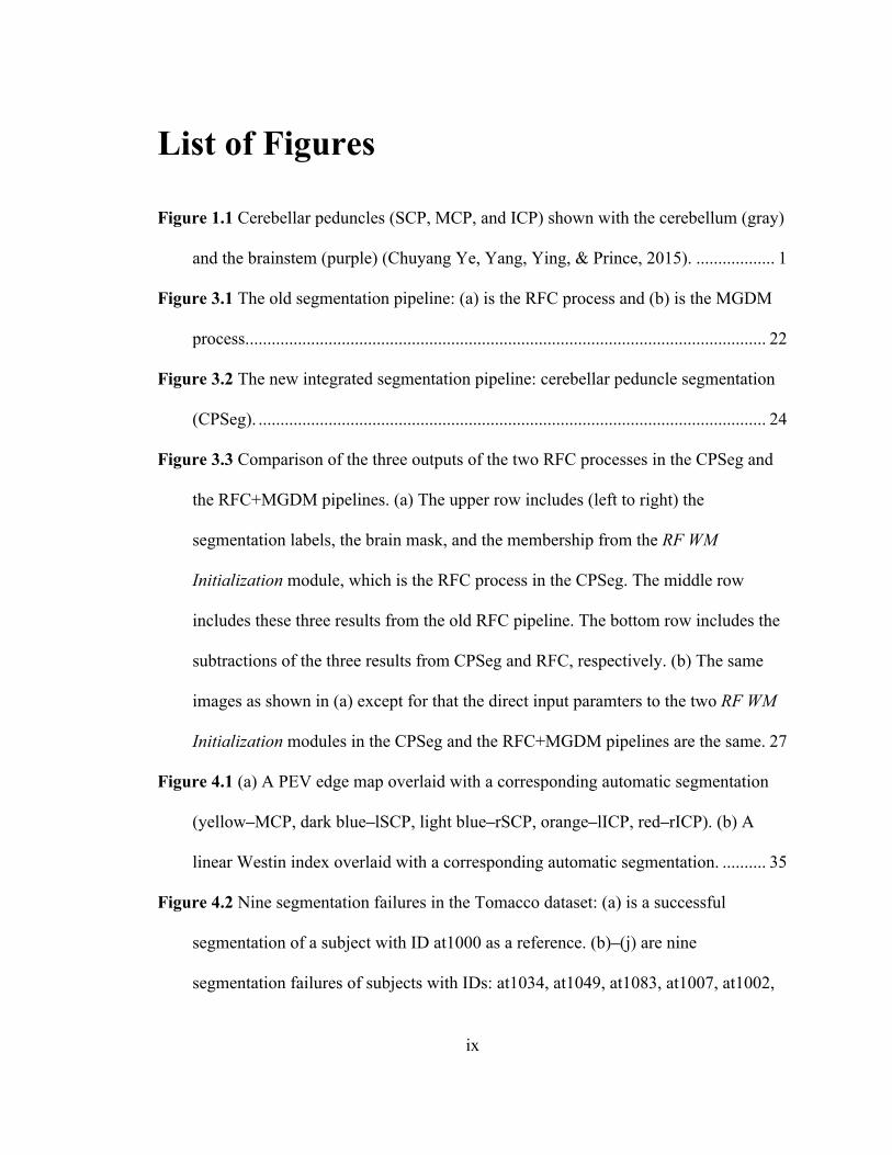
Figure 1.1 Cerebellar peduncles (SCP, MCP, and ICP) shown with the cerebellum (gray)

and the brainstem (purple) (Chuyang Ye, Yang, Ying, & Prince, 2015). .................. 1

Figure 3.1 The old segmentation pipeline: (a) is the RFC process and (b) is the MGDM

process. ...................................................................................................................... 22

Figure 3.2 The new integrated segmentation pipeline: cerebellar peduncle segmentation

(CPSeg). .................................................................................................................... 24

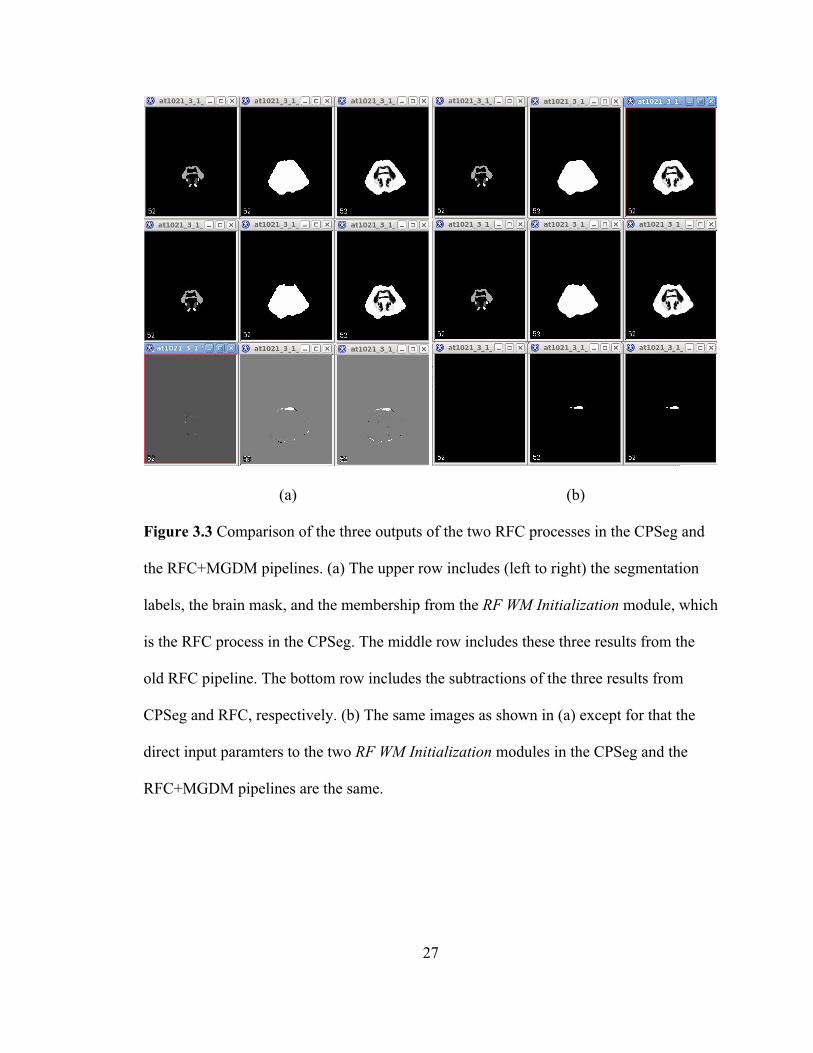
Figure 3.3 Comparison of the three outputs of the two RFC processes in the CPSeg and

the RFC+MGDM pipelines. (a) The upper row includes (left to right) the

segmentation labels, the brain mask, and the membership from the RF WM

Initialization module, which is the RFC process in the CPSeg. The middle row

includes these three results from the old RFC pipeline. The bottom row includes the

subtractions of the three results from CPSeg and RFC, respectively. (b) The same

images as shown in (a) except for that the direct input paramters to the two RF WM

Initialization modules in the CPSeg and the RFC+MGDM pipelines are the same. 27

Figure 4.1 (a) A PEV edge map overlaid with a corresponding automatic segmentation

(yellow–MCP, dark blue–lSCP, light blue–rSCP, orange–lICP, red–rICP). (b) A

linear Westin index overlaid with a corresponding automatic segmentation. .......... 35

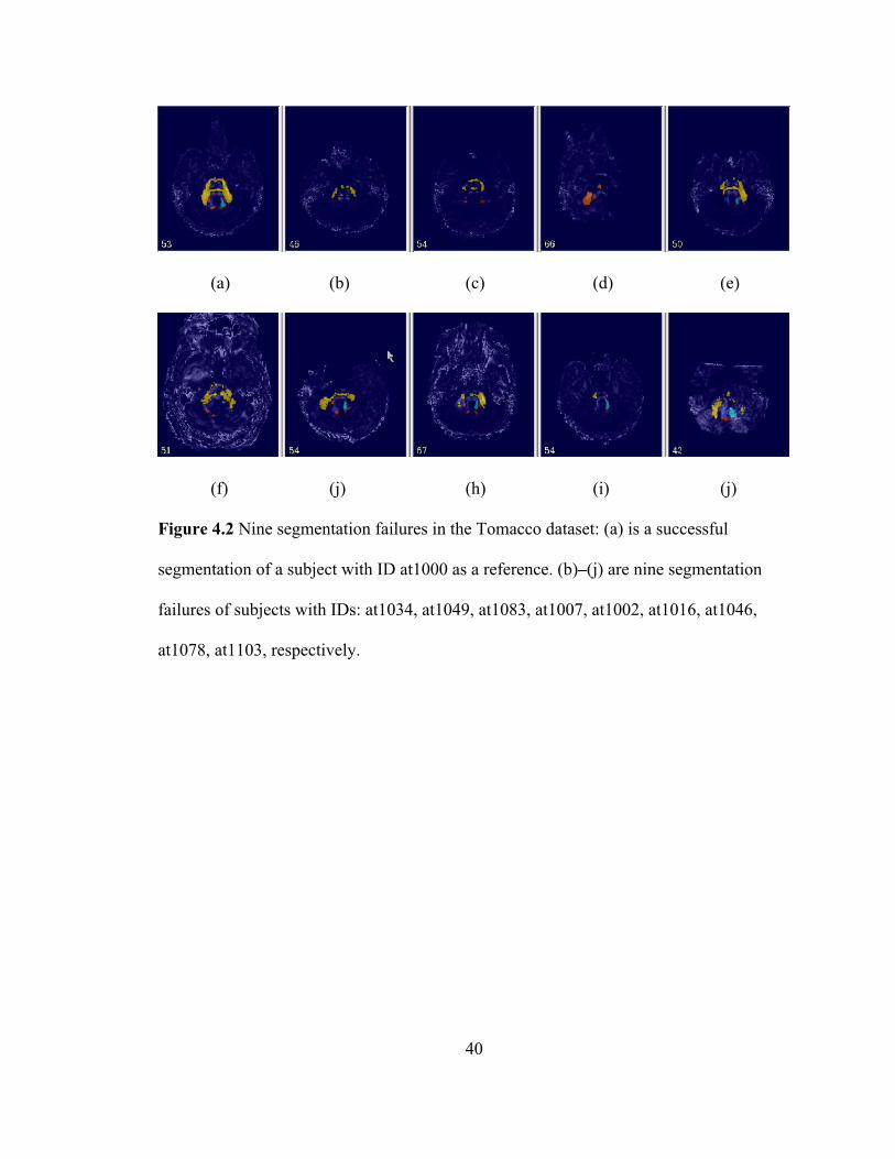
Figure 4.2 Nine segmentation failures in the Tomacco dataset: (a) is a successful

segmentation of a subject with ID at1000 as a reference. (b)–(j) are nine

segmentation failures of subjects with IDs: at1034, at1049, at1083, at1007, at1002,

x

at1016, at1046, at1078, at1103, respectively. ........................................................... 40

Figure 4.3 Six imperfect segmentations in the Tomacco dataset: (a)–(f) are image slices

of segmentation results from the subjects with IDs: at1032, at1056, at1041, at1080,

at1081, and at1086, respectively. (a), (b), (d), and (e): a small portion of MCPs are

cut off. (c) and (f): a small portion of lICP is cut off. ............................................... 41

Figure 4.4 Volumes of six CPs of manual delineations of 10 Tomacco datasets (red

boxes) and automatic segmentations of the 48 Tomaaco datasets (blue boxes),

respectively. .............................................................................................................. 46

Figure 4.5 Surface areas of six CPs of manual delineations of 10 Tomacco datasets (red


respectively. .............................................................................................................. 46

Figure 4.6 Means and SDs of FA and MD of the whole brains of the 48 Tomacco

datasets. ..................................................................................................................... 47

Figure 4.7 Means and SDs of the three Westin indices of the whole brains of the 48

Tomacco datasets. ..................................................................................................... 47

Figure 4.8 Brain mask features: volumes of the left, right, and whole brain masks (the

left 3 boxplots) and the symmetry of the brain masks (the rightest boxplot) of the 48

Tomacco datasets. ..................................................................................................... 48

Figure 5.1 Eight segmentation failures in the Kwyjibo dataset: (a) AT1275 with scan

time 04/02/2007, rICP is missing. (b) AT1532 with scan time 12/02/2009, dSCP is

missing. (c) AT1569 with scan time 10/01/2010, dSCP is missing. (d) AT1594 with

scan time 11/29/2012, dSCP is missing. (e) AT1061 with scan time 08/04/2008, a

large portion of MCP (yellow) is cut off. (f) AT1061 with scan time 03/06/2009, a

xi

large portion of MCP (yellow) is cut off. (g) AT1219 with scan time 07/30/2010,

failed to segment MCP and SCPs correctly. (h) AT1556 with scan time 08/02/2011,

rSCP is missing and MCP and lSCP are not correctly segmented. .......................... 55

Figure 5.2 Volumes of the six CPs of the 48 segmentations in the Tomacco dataset (red

boxes) and the 203 segmentations in the Kwyjibo dataset (blue boxes), respectively.

................................................................................................................................... 59

Figure 5.3 Surface areas of the six CPs of the 48 segmentations in the Tomacco dataset

(red boxes) and the 203 segmentations in the Kwyjibo dataset (blue boxes),

respectively. .............................................................................................................. 59


datasets (red boxes) and the 203 Kwyjibo datasets (blue boxes), respectively. ....... 60


Tomacco datasets (red boxes) and the 203 Kwyjibo datasets (blue boxes),

respectively. .............................................................................................................. 60

Figure 5.6 Brain mask features: volumes of the left, right, and whole brain masks and the

symmetry of the brain masks of the 48 Tomacco datasets (red boxes) and the 203

Kwyjibo datasets (blue boxes), respectively. ............................................................ 61

Figure 5.7 Volume differences of six CPs of 30 Tomacco segmentations using

CATNAP-v2 and CATNAP-v1, respectively. The results are obtained by subtracting

the volumes of CPs using CATNAP-v1 from those using CATNAP-v2. ................ 65

Figure 5.8 Histograms of the volume differences of the six CPs of 30 segmentations

using CATNAP-v2 and CATNAP-v1, respectively. The results are obtained by

subtracting the volumes of CPs using CATNAP-v1 from those using CATNAP-v2.

xii

................................................................................................................................... 66

Figure 5.9 (a) The registered segmentation result of at1020 using CATNAP-v1; (b) The

segmentation result of at1020 using CATNAP-v2; and (c) their subtraction. (d)The

MPRAGE image of at1020 and (e) the subtracted image overlaid with the MPRAGE

image. ........................................................................................................................ 66

Figure 5.10 Volumes of the six CPs of 46 reprocessed Tomacco datasets (red boxes) and

the 203 Kwyjibo datasets (blue boxes), respectively. ............................................... 70

Figure 5.11 Surface areas of the six CPs of the 46 reprocessed Tomacco datasets (red

boxes) and the 203 Kwyjibo datasets (blue boxes), respectively. ............................ 70

Figure 5.12 Means and SDs of FA and MD of the whole brains of the 46 reprocessed

Tomacco datasets (red boxes) and the 203 Kwyjibo datasets (blue boxes),

respectively. .............................................................................................................. 71


reprocessed Tomacco datasets (red boxes) and the 203 Kwyjibo datasets (blue

boxes), respectively. .................................................................................................. 71

Figure 5.14 Brain mask features: volumes of the left, right, and whole brain masks and

the symmetry of the brain masks of the 46 reprocessed segmentations in the

Tomacco dataset (red boxes) and the 203 segmentations in the Kwyjibo dataset (blue

boxes), respectively. .................................................................................................. 72

1

Chapter 1 Introduction

The cerebellar peduncles, which carry the inputs and outputs of the cerebellum,

are major white matter tracts connecting the cerebellum and other brain parts, including

the cerebral cortex and the spinal cord (Sivaswamy et al., 2010). They consist of superior

cerebellar peduncles (SCPs), the middle cerebellar peduncle (MCP), and the inferior

cerebellar peduncles (ICPs), as shown in Figure 1.1. Automatic segmentation and

quantification of the cerebellar peduncles is necessary for studying their structure and

function objectively and efficiently. Fortunately, diffusion tensor imaging (DTI) (Le

Bihan et al., 2001), which can characterize water diffusion magnitude and anisotropy

noninvasively, has made this goal achievable. However, while algorithms for

automatically segmenting the cerebellar peduncles based on DTI have been proposed,

none of the existing methods adequately segment the decussation of the SCPs (dSCP), the

region where the SCPs cross.

! Figure 1.1 Cerebellar peduncles (SCP, MCP, and ICP) shown with the cerebellum (gray)

and the brainstem (purple) (Chuyang Ye, Yang, Ying, & Prince, 2015).

2

To solve this problem, an automatic method to volumetrically segment the

cerebellar peduncles including the dSCP is proposed by Chuyang Ye et al.(Chuyang Ye

et al., 2015). This method consists of a random forest classifier (RFC) and a multi-object

geometric deformable model (MGDM). The random forest classifier uses features

extracted from the DTI scans to provide an initial segmentation of the peduncles. MGDM

is then used to refine the random forest classification, leading to smoother and more

accurate results. This method was evaluated using a leave-one-out cross-validation on

five control subjects and four patients with spinocerebellar ataxia type 6 (SCA6). Results

on these nine subjects indicate that the method is able to resolve the dSCPs and

accurately segment the cerebellar peduncles.

The focus of this thesis is on gaining a better understanding of the segmentation

performance of this CP segmentation method. This is important since the method will be

used on a much larger data set for scientific analysis. Usually performance evaluation of

automatic medical image segmentation methods is conducted by comparing the

segmentations with manual delineations (ground truth). However, while this approach

characterizes the performance in an average sense, when the method is run on new data

(for which no ground truth exists) it is highly desirable to be able to assess algorithm

failures so that these cases can be excluded from analysis or rerun with different

parameters. Considering the huge size of data and heavy workload of visual inspection,

finding a way to automatically and accurately detect algorithm failures is demanding.

In this thesis, we propose to carry out quality assurance for this automatic

segmentation method using outlier detection (Hodge & Austin, 2004). There is no

universally accepted definition for an outlier, but we will take the definition of Grubbs

3

(Grubbs, 1969) which stated that an outlying observation, or outlier, is one that appears to

deviate markedly from other members of the sample in which it occurs. Outlier detection

is a critical task in many safety critical environments as the outlier indicates abnormal

conditions from which significant performance degradation may result. Since outliers

arise because of many reasons such as human error, instrument error, natural deviation in

populations etc., how the outlier detection method detects and deals with the outlier

depends on the application area. Though outlier detection techniques have been applied

in areas such as fraud detection, activity monitoring, network performance, detecting

novelties in images etc., there is little research on detecting medical image segmentation

failures, and there is no work (of which we are aware) for the specific problem of the

automatic segmentation method of cerebellar peduncles presented in the paper (Ye et. al.

2015).

This thesis focuses on better understanding the performance of this CP

segmentation method using two outlier detection methods for quality assurance. One is a

simple univariate non-parametric method using box-whisker plots. The other is a

supervised classification method. Before outlier detection study, we first validated the

new segmentation pipeline used in this thesis. Then the univariate outlier detection

method using box-whisker plots is described. Automatic segmentation labels of a dataset

with 48 subjects were manually categorized as successful segmentations or segmentation

failures. Three kinds of features were extracted from the categorized failures and used for

failure detection. Next we applied both box-whisker plots and the supervised

classification method to a combined dataset with a total of 249 manually categorized (as

success or failure) automatic segmentation results. Four classifiers—linear discriminant

4

analysis (LDA), logistic regression (LR), support vector machine (SVM), and random

forest classifier (RFC) were used for failure detection in this combined dataset. Each

classifier’s performance was evaluated using a leave-one-out cross-validation. Results

show that the performances among the LDA, SVM and RFC are not very different and

LR performs worse than the other three classifiers.

In this chapter, the main contributions and the thesis organization are described.

5

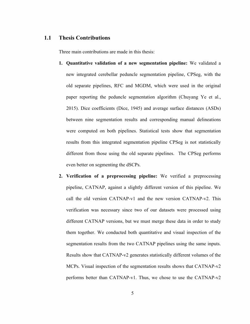
1.1 Thesis Contributions

Three main contributions are made in this thesis:

1. Quantitative validation of a new segmentation pipeline: We validated a

new integrated cerebellar peduncle segmentation pipeline, CPSeg, with the

old separate pipelines, RFC and MGDM, which were used in the original

paper reporting the peduncle segmentation algorithm (Chuyang Ye et al.,

2015). Dice coefficients (Dice, 1945) and average surface distances (ASDs)

between nine segmentation results and corresponding manual delineations

were computed on both pipelines. Statistical tests show that segmentation

results from this integrated segmentation pipeline CPSeg is not statistically

different from those using the old separate pipelines. The CPSeg performs

even better on segmenting the dSCPs.

2. Verification of a preprocessing pipeline: We verified a preprocessing

pipeline, CATNAP, against a slightly different version of this pipeline. We

call the old version CATNAP-v1 and the new version CATNAP-v2. This

verification was necessary since two of our datasets were processed using

different CATNAP versions, but we must merge these data in order to study

them together. We conducted both quantitative and visual inspection of the

segmentation results from the two CATNAP pipelines using the same inputs.

Results show that CATNAP-v2 generates statistically different volumes of the

MCPs. Visual inspection of the segmentation results shows that CATNAP-v2

performs better than CATNAP-v1. Thus, we chose to use the CATNAP-v2

6

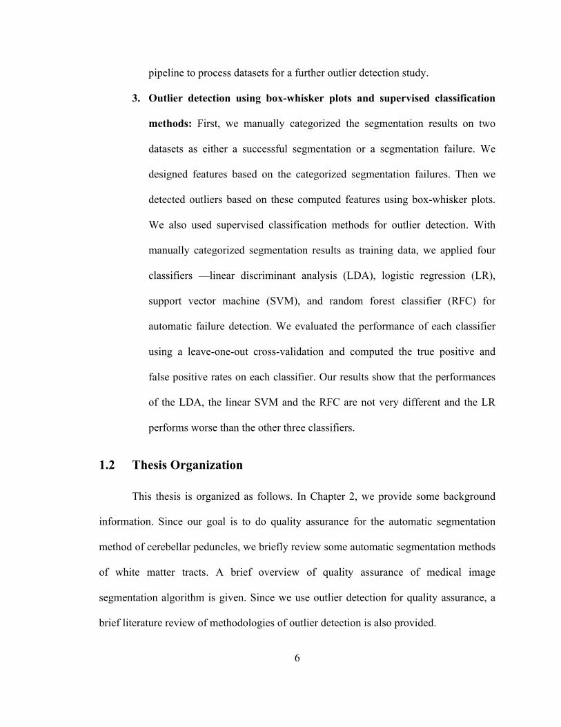
pipeline to process datasets for a further outlier detection study.

3. Outlier detection using box-whisker plots and supervised classification

methods: First, we manually categorized the segmentation results on two

datasets as either a successful segmentation or a segmentation failure. We

designed features based on the categorized segmentation failures. Then we

detected outliers based on these computed features using box-whisker plots.

We also used supervised classification methods for outlier detection. With

manually categorized segmentation results as training data, we applied four

classifiers —linear discriminant analysis (LDA), logistic regression (LR),

support vector machine (SVM), and random forest classifier (RFC) for

automatic failure detection. We evaluated the performance of each classifier

using a leave-one-out cross-validation and computed the true positive and

false positive rates on each classifier. Our results show that the performances

of the LDA, the linear SVM and the RFC are not very different and the LR

performs worse than the other three classifiers.

1.2 Thesis Organization

This thesis is organized as follows. In Chapter 2, we provide some background

information. Since our goal is to do quality assurance for the automatic segmentation

method of cerebellar peduncles, we briefly review some automatic segmentation methods

of white matter tracts. A brief overview of quality assurance of medical image

segmentation algorithm is given. Since we use outlier detection for quality assurance, a

brief literature review of methodologies of outlier detection is also provided.

7

In Chapter 3, we present quantitative validation of the integrated new

segmentation pipeline, namely the CPSeg. We first introduce the old segmentation

pipeline consisting of two separate pipelines (RFC and MGDM) and the CPSeg. Then,

we compare the two pipelines and show the differences between their segmentation

results. Next, for both pipelines, we report the computed Dice coefficients and average

surface distances (ASDs) between the segmentation results and manual delineations. We

used a Paired student’s t -test and a Wilcoxon signed-rank test to statistically compare

the Dice coefficients and ASDs; results show that the new segmentation pipeline is not

statistically different from the old one.

Chapter 4 presents results on the use of a simple outlier detection method applied

to a dataset including 48 subjects with both healthy controls and subjects with ataxia. The

segmentation results in this dataset were manually categorized as successful

segmentations or segmentation failures. We then computed several statistics and

evaluated informally whether these features seemed capable of identifying the poor

segmentation results. Lastly, we detect outliers in this dataset by selected features and

evaluated the performance of each feature.

In the research reported in Chapter 5, we conduct outlier detection on two datasets

using both box-whisker plots and supervised classification methods to study the

performance of the automatic segmentation algorithm. We first studied the segmentation

algorithm’s performance on a data set with 203 subjects including both healthy controls

and patients with ataxia. We manually categorized these segmentation labels as

successful segmentations or segmentation failures and detected outliers using boxplots.

We found that the distributions of some features in the the Kwyjibo dataset are

8

significantly different from those in the Tomacco dataset and features deemed effective in

the Tomacco dataset are not all able to detect outliers in the Kwyjibo dataset. Since the

Kwyjibo dataset was processed using an updated preprocessing pipeline CATNAP-v2

with the CPSeg while Tomacco dataset were processed using CATNAP-v1 with the

CPSeg, we reprocessed the Tomacco dataset using the CATNAP-v2. Before that, we

verified the CATNAP-v2. Last, we combined the reprocessed Tomacco and Kwyjibo

datasets using the CATNAP-v2 and the CPSeg. We trained four classifiers—linear

discriminant analysis (LDA), logistic regression (LR), support vector machine (SVM),

and random forest classifier (RFC) for automatic failure detection and evaluated the

performance of each classifier using a leave-one-out cross-validation. We also computed

the true positive and false positive rates of each classifier. Results show that the

performances among the LDA, SVM and RFC are not significantly different and LR

performs worse than the other three classifiers.

In the final chapter, we summarize the main contributions and conclusions of this

thesis. We also highlight some future work about this project.

9

Chapter 2 Background

The target of this thesis is quality assurance for automatic segmentation algorithm

of cerebellar peduncles developed by Ye et al. (Chuyang Ye et al., 2015). The general

background and theory of this algorithm therefore is given first. Then a brief overview of

quality assurance methods in medical image analysis is presented. Lastly, we introduce

methodologies for outlier detection.

2.1 Automatic Segmentation Method of Cerebellar Peduncles

The cerebellum has three peduncles: the superior cerebellar peduncles (SCPs), the

middle cerebellar peduncles (MCPs), and the inferior cerebellar peduncles (ICPs). The

SCPs consists mainly of efferent fibers from the cerebellum to the thalamus and red

nucleus. The left and right SCPs cross each other in a region called decussation of the

SCP (dSCP) in the midbrain. The fibers then head toward the red nuclei on the opposite

side, where some fibers terminate but most continue to the thalamus (Perrini, Tiezzi,

Castagna, & Vannozzi, 2013).The MCPs consists of centripetal fibers, connecting the

cerebellum to the pons. The ICPs primarily contain afferent fibers from the medulla, as

well as efferent fibers to the vestibular nuclei (Mori, Wakana, Van Zijl, & Nagae-

Poetscher, 2005).

Cerebellar peduncles can be affected by neurological diseases including

spinocerebellar ataxia (Murata et al., 1998; Ying et al., 2009), Wilson disease (King et

al., 1996; Magalhaes et al., 1994), schizophrenia (F. Wang et al., 2003), and multiple

10

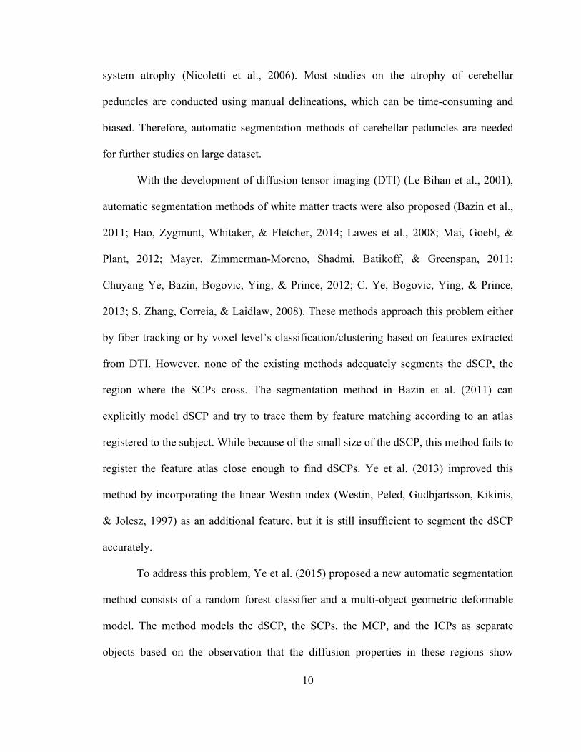
system atrophy (Nicoletti et al., 2006). Most studies on the atrophy of cerebellar

peduncles are conducted using manual delineations, which can be time-consuming and

biased. Therefore, automatic segmentation methods of cerebellar peduncles are needed

for further studies on large dataset.

With the development of diffusion tensor imaging (DTI) (Le Bihan et al., 2001),

automatic segmentation methods of white matter tracts were also proposed (Bazin et al.,

2011; Hao, Zygmunt, Whitaker, & Fletcher, 2014; Lawes et al., 2008; Mai, Goebl, &

Plant, 2012; Mayer, Zimmerman-Moreno, Shadmi, Batikoff, & Greenspan, 2011;

Chuyang Ye, Bazin, Bogovic, Ying, & Prince, 2012; C. Ye, Bogovic, Ying, & Prince,

2013; S. Zhang, Correia, & Laidlaw, 2008). These methods approach this problem either

by fiber tracking or by voxel level’s classification/clustering based on features extracted

from DTI. However, none of the existing methods adequately segments the dSCP, the

region where the SCPs cross. The segmentation method in Bazin et al. (2011) can

explicitly model dSCP and try to trace them by feature matching according to an atlas

registered to the subject. While because of the small size of the dSCP, this method fails to

register the feature atlas close enough to find dSCPs. Ye et al. (2013) improved this

method by incorporating the linear Westin index (Westin, Peled, Gudbjartsson, Kikinis,

& Jolesz, 1997) as an additional feature, but it is still insufficient to segment the dSCP

accurately.

To address this problem, Ye et al. (2015) proposed a new automatic segmentation

method consists of a random forest classifier and a multi-object geometric deformable

model. The method models the dSCP, the SCPs, the MCP, and the ICPs as separate

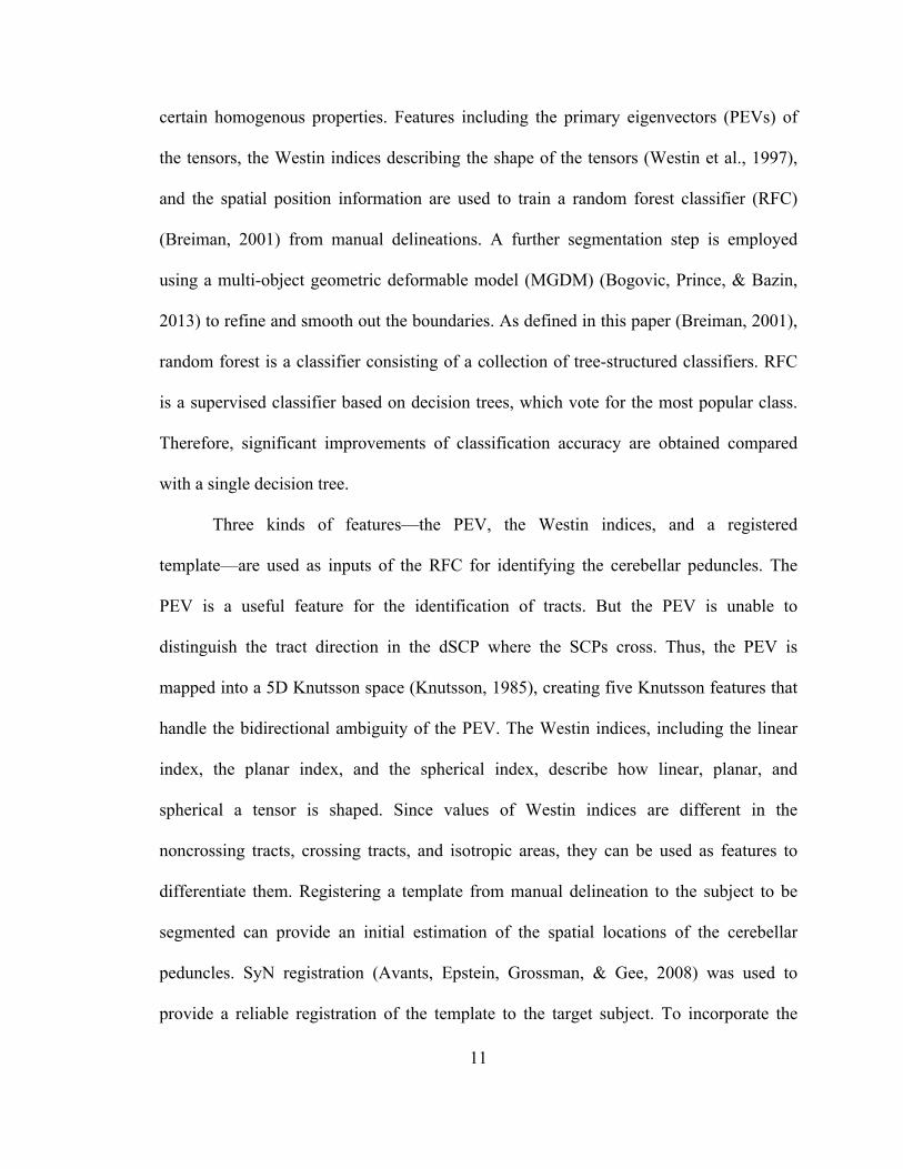
objects based on the observation that the diffusion properties in these regions show

11

certain homogenous properties. Features including the primary eigenvectors (PEVs) of

the tensors, the Westin indices describing the shape of the tensors (Westin et al., 1997),

and the spatial position information are used to train a random forest classifier (RFC)

(Breiman, 2001) from manual delineations. A further segmentation step is employed

using a multi-object geometric deformable model (MGDM) (Bogovic, Prince, & Bazin,

2013) to refine and smooth out the boundaries. As defined in this paper (Breiman, 2001),

random forest is a classifier consisting of a collection of tree-structured classifiers. RFC

is a supervised classifier based on decision trees, which vote for the most popular class.

Therefore, significant improvements of classification accuracy are obtained compared

with a single decision tree.

Three kinds of features—the PEV, the Westin indices, and a registered

template—are used as inputs of the RFC for identifying the cerebellar peduncles. The

PEV is a useful feature for the identification of tracts. But the PEV is unable to

distinguish the tract direction in the dSCP where the SCPs cross. Thus, the PEV is

mapped into a 5D Knutsson space (Knutsson, 1985), creating five Knutsson features that

handle the bidirectional ambiguity of the PEV. The Westin indices, including the linear

index, the planar index, and the spherical index, describe how linear, planar, and

spherical a tensor is shaped. Since values of Westin indices are different in the

noncrossing tracts, crossing tracts, and isotropic areas, they can be used as features to

differentiate them. Registering a template from manual delineation to the subject to be

segmented can provide an initial estimation of the spatial locations of the cerebellar

peduncles. SyN registration (Avants, Epstein, Grossman, & Gee, 2008) was used to

provide a reliable registration of the template to the target subject. To incorporate the

12

information from SyN registration into the RFC, signed distance functions (SDFs) were

calculated from the transformed labels. SDFs can indicate how far a voxel of the target

subject is from the registered labels, serving as spatial information of the spatial locations

of cerebellar peduncles.

The RFC provides an initial classification of the cerebellar peduncles, but since 1)

the RFC applies to each voxel independently and 2) the RFC training may have

unbalanced samples (where the more numerous classes tend to be favored in RFC

decisions producing a bias in the sizes), a further step for refining the initial classification

is required. Therefore, MGDM (Bogovic et al., 2013) was applied to provide both spatial

smoothness and additional fidelity to the data.

2.2 Quality Assurance in Medical Imaging Field

Extensive, consistent, and regular QA is an essential part of medical imaging. QA

in magnetic resonance imaging (MRI) field is mainly focused on the imaging systems

(Gallichan et al., 2010; Ihalainen, Sipila, & Savolainen, 2004; Z. J. Wang, Seo, Chia, &

Rollins, 2011; Yung, Stefan, Reeve, & Stafford, 2015), DTI image quality (Asman,

Lauzon, & Landman, 2013; Lauzon et al., 2013), and algorithms of medical image

processing and analysis (Rodrigues et al., 2012; Saenz, Kim, Chen, Stathakis, & Kirby,

2015; Sharpe & Brock, 2008). The quality of imaging system can affect the quality of the

output images, which as inputs can affect the final results of algorithms of medical

imaging processing and analysis. Quality assurance of the three aspects is therefore

dependent to some extent.

Quality assurance for the medical imaging systems is generally conducted by

13

comparing parameters of images obtained from these systems using phantoms. Ihalaine et

al (2004) proposed to develop a long-term quality control protocol for the six magnetic

resonance imagers in their organization in order to assure that they fulfill the same basic

image quality requirements. They used the same Eurospin phantom set and compared 11

identical imaging parameters with each imager. They are image uniformity, ghosting,

SNR and its uniformity, geometric distortion, slice thickness, slice position, slice wrap,

resolution, and T1 and T2 accuracy. Results proved that the six imagers were operating at

a performance level adequate for clinical imaging.

Wang et al. (2011) presented a similar quality assurance procedure for routine

clinical DTI using the widely available American College of Radiology (ACR) head

phantom. They analyzed the data acquired at 1.5 and 3.0 T on whole body clinical MRI

scanners and compared parameters including 1) the signal-to-noise ratio (SNR) at the

center and periphery of the phantom, 2) image distortion by EPI readout relative to spin

echo imaging, 3) distortion of high-b images relative to the b=0 image caused by

diffusion encoding, and 4) determination of fractional anisotropy (FA) and mean

diffusivity (MD) measured with region-of-interest (ROI) and pixel-based approaches.

In Yung et al (2015), a semi-automated, open source MRI QA program for multi-

unit institutions was developed. With the reviewable database of phantom measurements,

historical data can be reviewed to compare previous year data and to inspect for trends.

The QA approach in this paper is the same as the previous ones. Measurements using

phantoms assess geometric accuracy and linearity, position accuracy, image uniformity,

signal, noise, ghosting, transmit gain, center frequency, and magnetic field drift.

Currently, quality inspection of DTI data has relied on visual inspection and

14

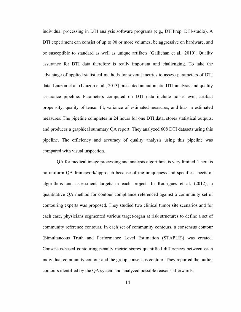
individual processing in DTI analysis software programs (e.g., DTIPrep, DTI-studio). A

DTI experiment can consist of up to 90 or more volumes, be aggressive on hardware, and

be susceptible to standard as well as unique artifacts (Gallichan et al., 2010). Quality

assurance for DTI data therefore is really important and challenging. To take the

advantage of applied statistical methods for several metrics to assess parameters of DTI

data, Lauzon et al. (Lauzon et al., 2013) presented an automatic DTI analysis and quality

assurance pipeline. Parameters computed on DTI data include noise level, artifact

propensity, quality of tensor fit, variance of estimated measures, and bias in estimated

measures. The pipeline completes in 24 hours for one DTI data, stores statistical outputs,

and produces a graphical summary QA report. They analyzed 608 DTI datasets using this

pipeline. The efficiency and accuracy of quality analysis using this pipeline was

compared with visual inspection.

QA for medical image processing and analysis algorithms is very limited. There is

no uniform QA framework/approach because of the uniqueness and specific aspects of

algorithms and assessment targets in each project. In Rodrigues et al. (2012), a

quantitative QA method for contour compliance referenced against a community set of

contouring experts was proposed. They studied two clinical tumor site scenarios and for

each case, physicians segmented various target/organ at risk structures to define a set of

community reference contours. In each set of community contours, a consensus contour

(Simultaneous Truth and Performance Level Estimation (STAPLE)) was created.

Consensus-based contouring penalty metric scores quantified differences between each

individual community contour and the group consensus contour. They reported the outlier

contours identified by the QA system and analyzed possible reasons afterwards.

15

Seenz et al. (2015) proposed to determine how detailed a physical phantom needs

to be to accurately perform QA for a deformable image registration (DIR) algorithm.

Virtual prostate and head-and-neck phantoms, made from patient images, were used for

this study. Both sets consist of an undeformed and deformed image pair. They found that

a higher number of tissue levels creates more contrast in an image and enables DIR

algorithms to produce more accurate results.

QA approaches in medical imaging systems, DTI data quality, and algorithms are

reviewed above. Overall, QA is important yet not fully studied for medical imaging field.

More efficient, accurate, and automatic QA approaches remain to be further developed.

This thesis considers a particular approach for a specific algorithm, and therefore

contributes to the general state of knowledge in quality assurance for medical image

analysis.

2.3 Outlier Detection Methodologies

The presence of outliers can be a problem for data analysis in many fields. Outlier

identification herein is an important part of data screening process to detect and/or

remove consequent abnormal observations (Hodge & Austin, 2004). Outliers can results

from various reasons such as human error, systematic errors, fraudulent behavior, or

simply natural deviations in populations. Considering there is no universally accepted

definition of an outlier, we take the definition of Grubbs (1969), who defined an outlying

observation, or outlier, to be “one that appears to deviate markedly from other members

of the sample in which it occurs”. This review focuses on a general overview of outlier

detection methodologies rather than a specific method for a specific problem. Outlier

16

detection methods originated from statistics and machine learning fields are introduced

briefly.

Statistical methods are widely used in outlier detection. For univariate outlier

detection, Grubbs (1969) presented several recommended criteria for determining outliers.

One of these criteria is the Z value, which is the difference between the mean of data and

the query value divided by the standard deviation. The Z value is then compared with a

1% or 5% significance level for outlier detection. All parameters are directly calculated

from the data. Large data number herein can represent the sample statistically better.

Another very simple and fast statistical outlier detection technique proposed by

Laruikkala et al. (Laurikkala et al., 2000) is box-whisker plot to pinpoint outliers. Box

plots give the lower and higher extremes, lower and higher quartiles, median of data, and

outliers. The outliers are data outside of the 1.5 x interquartile range beyond the lower

and upper extremes. The whisker value 1.5 can be adjusted according to different datasets.

Box plots require no data distribution assumption but need a predefined range of outliers.

For multivariate outlier detection, Mahalanobis distances (De Maesschalck,

Jouan-Rimbaud, & Massart, 2000) is the primary choice for many cases. This distance

measure incorporates the dependencies between the variables, which is essential in

multivariate outlier detection. Other distance metrics, such as Euclidean distance using

only location information, are not as accurate as Mahalanobis distance. While the

Mahalanobis distance can be computationally expensive compared with the Euclidean

distance since it requires an entire dataset to identify the variable correlations. K-nearest

neighbor (KNN) for outlier detection calculates the nearest neighbors of a data using a

proper distance metric, such as Euclidean distance or Mahalanobis distance. It is a

17

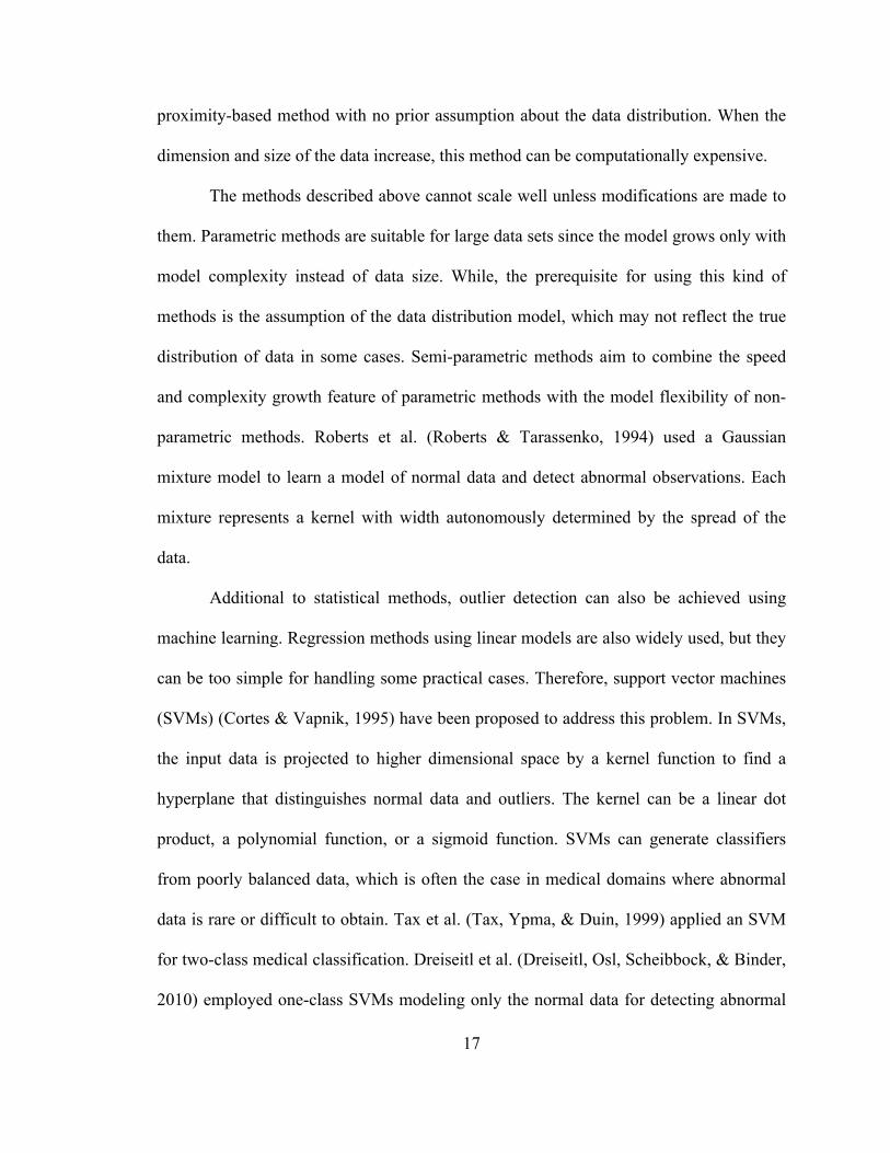
proximity-based method with no prior assumption about the data distribution. When the

dimension and size of the data increase, this method can be computationally expensive.

The methods described above cannot scale well unless modifications are made to

them. Parametric methods are suitable for large data sets since the model grows only with

model complexity instead of data size. While, the prerequisite for using this kind of

methods is the assumption of the data distribution model, which may not reflect the true

distribution of data in some cases. Semi-parametric methods aim to combine the speed

and complexity growth feature of parametric methods with the model flexibility of non-

parametric methods. Roberts et al. (Roberts & Tarassenko, 1994) used a Gaussian

mixture model to learn a model of normal data and detect abnormal observations. Each

mixture represents a kernel with width autonomously determined by the spread of the

data.

Additional to statistical methods, outlier detection can also be achieved using

machine learning. Regression methods using linear models are also widely used, but they

can be too simple for handling some practical cases. Therefore, support vector machines

(SVMs) (Cortes & Vapnik, 1995) have been proposed to address this problem. In SVMs,

the input data is projected to higher dimensional space by a kernel function to find a

hyperplane that distinguishes normal data and outliers. The kernel can be a linear dot

product, a polynomial function, or a sigmoid function. SVMs can generate classifiers

from poorly balanced data, which is often the case in medical domains where abnormal

data is rare or difficult to obtain. Tax et al. (Tax, Ypma, & Duin, 1999) applied an SVM

for two-class medical classification. Dreiseitl et al. (Dreiseitl, Osl, Scheibbock, & Binder,

2010) employed one-class SVMs modeling only the normal data for detecting abnormal

18

subjects in melanoma prognosis. They compared their methods with a two-class

classification method and came to the conclusion that their method can be used as an

alternative.

Statistical methods primarily focus on real-valued data and require cardinal or

ordinal data to allow vector distances to be calculated. Methods derived from machine

learning can handle categorical data with no ordering. For example decision trees are

robust and do not require any prior knowledge of the distribution of the data, but they

generate simple class boundaries compared with the complex class boundaries by SVM

or neural networks. To improve the accuracy, ensemble classification methods, for

example, random forests, were proposed (Breiman, 2001). This classification method is

described in Section 2.1, so no additional theory is described here. Generally, the random

forest classifier consisting of a collection of decision trees, and performs better than a

single decision tree.

Though outlier detection has been applied in many fields such as fraud detection,

activity monitoring, network performance, structural defect detection, time-series

monitoring, medical condition monitoring etc., there is very limited study of quality

assurance using outlier detection for medical image segmentation algorithms.

Considering our case with only 249 data and the relatively low dimension of variables

(number of features < 30), we applied the simple statistical method using box-whisker

plots first. Then with available ground truth for segmentation failures and effective

features for indicating outliers, we moved to classification methods and utilized several

classifiers including SVM and random forest classifier for detecting outliers. Some data

mining algorithms based on tree structured indices and cluster hierarchies (T. Zhang,

19

Ramakrishnan, & Livny, 1996) are robust, but are specifically optimized for clustering

large data set. Therefore, it is not proper for our case.

20

Chapter 3 Validation of the New

Algorithm Pipeline

There are two segmentation pipelines: the original pipeline consisting of two

separate pipelines used in the paper reporting the automatic segmentation method of

cerebellar peduncles (Chuyang Ye et al., 2015) and the new integrated pipeline, CPSeg,

used in this thesis. A dataset containing 48 subjects were first preprocessed using a

pipeline for registration and estimating diffusion tensors. Then the computed tensors were

processed using the old segmentation pipeline, namely RFC+MGDM, and the new

CPSeg pipeline. Six segmentation labels of the CPs were the final outputs of the two

segmentation pipelines. We then compared the segmentation labels of the two pipelines

and found they were different. To guarantee the differences are not statistically

significant, we did a quantitative validation of the CPSeg pipeline. We computed the

Dice coefficients and average surface distances (ASDs) between segmentation labels and

the corresponding manual delineations of 10 subjects in this dataset with 48 subjects. We

then used a Paired student’s t -test and a Wilcoxon signed-rank test to statistically

compare the Dice coefficients and ASDs; results show that the segmentation labels using

the new segmentation pipeline is not statistically different from those using the old

pipeline. The details are provided in this chapter.

21

3.1 Algorithm Pipelines

3.1.1 CATNAP

CATNAP (Landman, Farrell, Patel, Mori, & Prince, 2007), short for

Coregistration, Adjustment and Tensor-solving, a Nicely Automated Program, is a data

preprocessing pipeline for Philips DTI (PAR/REC) and MRI data. CATNAP can adjust

diffusion gradient directions for scanner settings, correct motions and eddy current

artifacts, and compute diffusion tensors and parameters such as fractional anisotropy

(FA), mean diffusivity (MD), and Westin indices. The computed diffusion tensors are

used as inputs to the segmentation pipeline (RFC+MGDM and CPSeg). The CATNAP

pipeline used in Ye et al. (2015) has no distortion correction function. We call it

CATNAP-v1 to differentiate it from a slightly different version, CATNAP-v2 (described

in Chapter 5), which was used for another data set. The two CATNAPs, RFC+MGDM,

and CPSeg pipelines were all implemented using the Java Image Science Toolkit (JIST)

(Lucas et al., 2010). JIST is an algorithm development framework, which supports java-

based rapid prototyping, improving the efficiency of evaluating new algorithms.

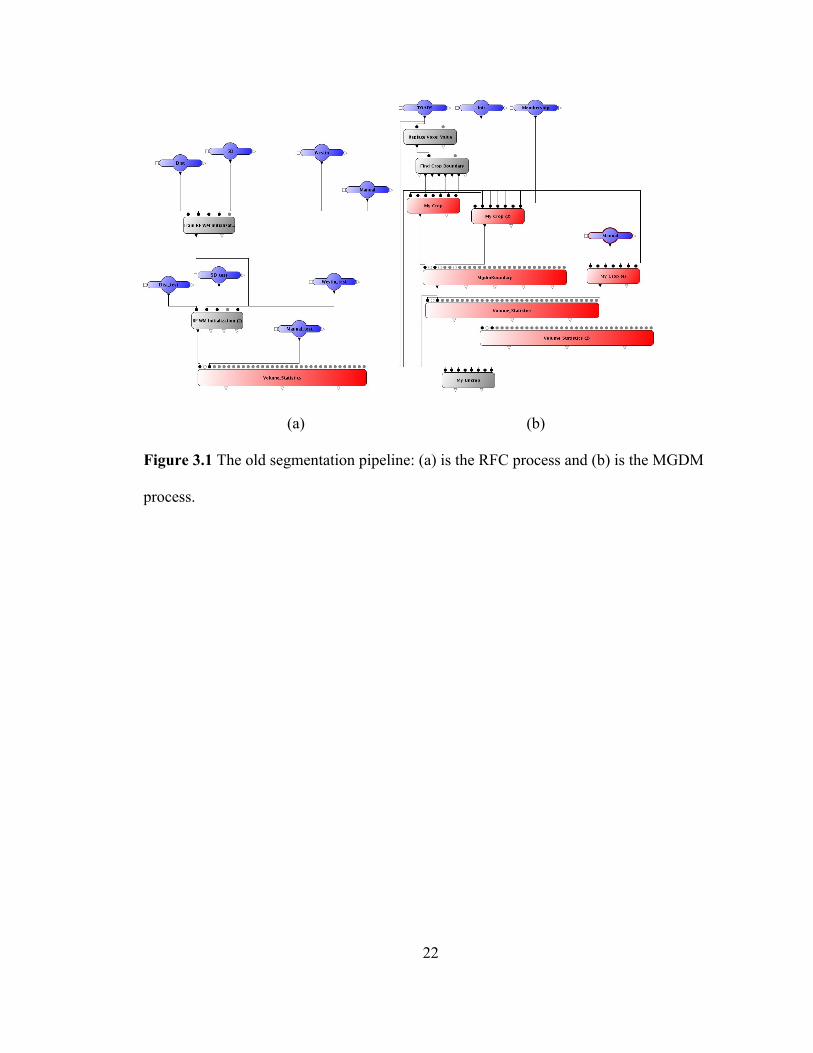
3.1.2 The segmentation pipelines

The old segmentation pipeline (RFC+MGDM) consists of a RFC process and a

MGDM processes, as shown in Figure 3.1.

22

(a) (b)

Figure 3.1 The old segmentation pipeline: (a) is the RFC process and (b) is the MGDM

process.

23

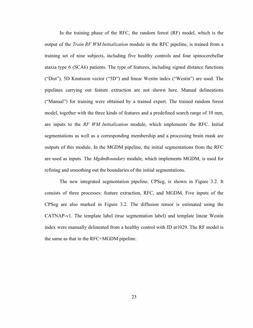
In the training phase of the RFC, the random forest (RF) model, which is the

output of the Train RF WM Initialization module in the RFC pipeline, is trained from a

training set of nine subjects, including five healthy controls and four spinocerebellar

ataxia type 6 (SCA6) patients. The type of features, including signed distance functions

(“Dist”), 5D Knutsson vector (“5D”) and linear Westin index (“Westin”) are used. The

pipelines carrying out feature extraction are not shown here. Manual delineations

(“Manual”) for training were obtained by a trained expert. The trained random forest

model, together with the three kinds of features and a predefined search range of 10 mm,

are inputs to the RF WM Initialization module, which implements the RFC. Initial

segmentations as well as a corresponding membership and a processing brain mask are

outputs of this module. In the MGDM pipeline, the initial segmentations from the RFC

are used as inputs. The MgdmBoundary module, which implements MGDM, is used for

refining and smoothing out the boundaries of the initial segmentations.

The new integrated segmentation pipeline, CPSeg, is shown in Figure 3.2. It

consists of three processes: feature extraction, RFC, and MGDM. Five inputs of the

CPSeg are also marked in Figure 3.2. The diffusion tensor is estimated using the

CATNAP-v1. The template label (true segmentation label) and template linear Westin

index were manually delineated from a healthy control with ID at1029. The RF model is

the same as that in the RFC+MGDM pipeline.

25

3.2 Comparison of Segmentation labels

Theoretically, the new and old pipelines should be the same since the new one is

just a composition of the two old ones. To test this hypothesis, we processed a data set

with 48 subjects using CATNAP-v1 and CPSeg and compared the segmentation results

with those processed by CATNAP-v1 and RFC+MGDM.

3.2.1 Description of the Tomacco dataset

The Tomacco dataset contains a total of 48 subjects: 18 healthy controls， 6

patients with SCA6, and 24 patients with other neurological diagnoses that affect the

cerebellum. Each subject has a set of several DTI and magnetization-prepared rapid

acquisition gradient echo (MPRAGE) scans. Diffusion weighted images (DWIs) were

acquired using a multi-slice, single-shot EPI sequence on a 3T MR scanner (Intera,

Philips Medical Systems, Netherlands). The sequence has 32 gradient directions and one

b0 image. The b value is 700 s/mm2. The resolution in the XY plane is 2.2mm × 2.2mm

with 96 × 96 slices. The resolution of the output images generated by the scanner is

0.828mm × 0.828mm × 2.2mm. We registered the MPRAGE images to MNI space to get

the isotropic resolution 1mm.

We successfully processed all the 48 Tomacco datasets using the CPSeg with

estimated tensors as inputs computed using the CATNAP-v1. It takes around 2.5 hours to

process one subject using the CATNAP-v1 and 40 minutes using the CPSeg. The total

time for processing one subject is around 3 hours. For each subject, the final outputs of

the CPSeg are six segmentation labels 1–6 representing the left SCP (lSCP), right SCP

26

(rSCP), dSCP, MCP, left ICP (lICP), and right ICP (rICP), respectively. The Tomacco

dataset had been processed using the RFC+MGDM with tensors computed using the

CATNAP-v1. In the following section we compare the segmentations labels from the

CPSeg and the RFC+MGDM.

3.2.2 Comparison results

We used Linux command “diff” to compare estimated tensors from the

CATNAP-v1 and the final segmentation labels by using the two segmentation pipelines.

Results show that, the estimated tensors we processed using the CATNAP-v1 were

exactly the same as those processed by Ye using the same CATNAP-v1. While, the final

segmentation labels by using the CPSeg were different from those by using the

RFC+MGDM.

Since final segmentation labels of the MGDM process directly depends on the

outputs of the RFC process, we then compared the three outputs–the initial segmentation

labels, the brain masks, and the memberships–of the two RFC processes in the

RFC+MGDM and the CPSeg pipelines. Figure 3.3(a) shows that these three results from

the two RF WM Initialization modules, which implements the two RFC processes in the

two segmentation pipelines, are different.

28

Then we checked the two RF WM Initialization modules and found their versions

and parameters of inputs were different. To figure out whether the different module

versions caused the different outputs, we ran the two modules given the same inputs and

compared their three outputs. Results showed that the segmentation labels of the two

modules were the same, while the brain masks and the memberships were still different.

A portion of the brain masks and memberships generated by the RF WM Initialization

module in the RFC+MGDM pipeline were chopped, as shown in Figure 3.3(b). This

indicates that the two RF WM Initialization modules in the two segmentation pipelines

are indeed different in some way.

We checked all the other modules before the RF WM Initialization in a similar

way and found another reason for the differences of the final segmentation labels of the

CPSeg and RFC+MGDM pipelines. We found that, given the same inputs, the CP

Template Registration module in the CPSeg pipeline generated a different registered

template compared with that by using SyN registration (Avants et al., 2008) in the

RFC+MGDM pipeline. The CP Template Registration module registers the template

label and the template linear Westin index of a subject with ID at1029 to the target linear

Westin index of a subject to be segmented and creates a registered template. Since this

registered template is used for calculating the SDFs, the feature of spatial location

information of cerebellar peduncles used to train the RFC in the CPSeg pipeline, it can

influence the final segmentation results. Thus, the differences between the registration

module (CP Template Registration) in the CPSeg pipeline and the corresponding SyN

registration process in the RFC+MGDM pipeline is a reason for the final different

segmentation labels in the two segmentation pipelines.

29

In conclusion, the new segmentation pipeline CPSeg cannot generate the same

segmentation labels as the old pipeline RFC+MGDM. Two possible reasons for it were

analyzed. Then we need to validate the segmentation results using the tow pipelines to

guarantee they are not statistically significant. Although the results are different, it is

possible that the differences are not statistically significant relative to the final quantities

that we will compare in population studies. For this reason we next analyzed the statistics

of the two final segmentation results by using the two pipelines, and these results are

described in the following section.

3.3 Statistical Tests

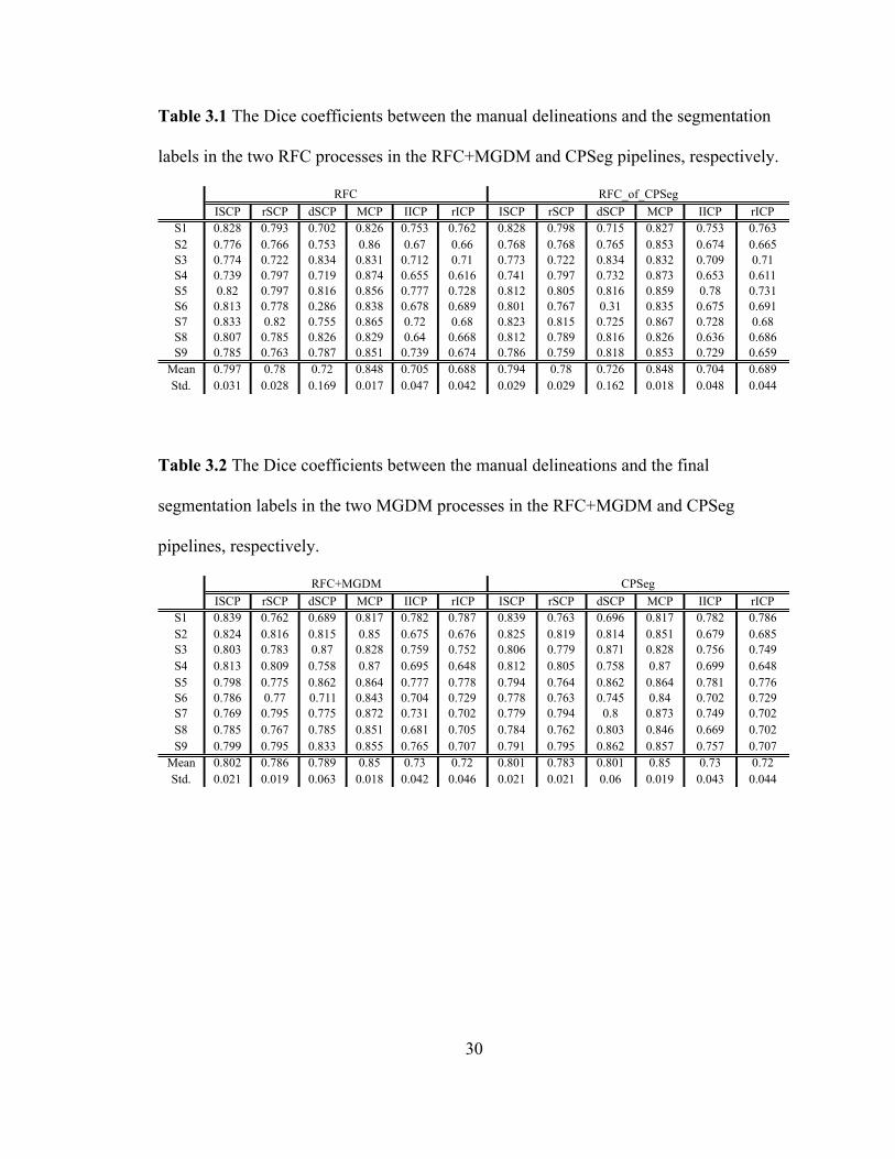
3.3.1 Tests on the Dice coefficients

We first calculated the Dice coefficients (Dice, 1945) between manual

delineations and the initial segmentation labels in the two RFC processes in the

RFC+MGDM and CPSeg pipelines, respectively. We then calculated the Dice

coefficients between manual delineations and the final segmentations from the two

MGDM processes in the RFC+MGDM and CPSeg pipelines, respectively. The two

groups of Dice coefficients are shown in Tables 3.1 and 3.2, respectively. For

convenience, the RFC segmentation results and the final segmentation results after

MGDM refinement are called “RFC” and “RFC + MGDM” in the RFC+MGDM pipeline

and called “RFC_of_CPSeg” and “CPSeg” in the CPSeg pipeline.

30

Table 3.1 The Dice coefficients between the manual delineations and the segmentation

labels in the two RFC processes in the RFC+MGDM and CPSeg pipelines, respectively.

ISCP rSCP dSCP MCP IICP rICP ISCP rSCP dSCP MCP IICP rICPS1 0.828 0.793 0.702 0.826 0.753 0.762 0.828 0.798 0.715 0.827 0.753 0.763S2 0.776 0.766 0.753 0.86 0.67 0.66 0.768 0.768 0.765 0.853 0.674 0.665S3 0.774 0.722 0.834 0.831 0.712 0.71 0.773 0.722 0.834 0.832 0.709 0.71S4 0.739 0.797 0.719 0.874 0.655 0.616 0.741 0.797 0.732 0.873 0.653 0.611S5 0.82 0.797 0.816 0.856 0.777 0.728 0.812 0.805 0.816 0.859 0.78 0.731S6 0.813 0.778 0.286 0.838 0.678 0.689 0.801 0.767 0.31 0.835 0.675 0.691S7 0.833 0.82 0.755 0.865 0.72 0.68 0.823 0.815 0.725 0.867 0.728 0.68S8 0.807 0.785 0.826 0.829 0.64 0.668 0.812 0.789 0.816 0.826 0.636 0.686S9 0.785 0.763 0.787 0.851 0.739 0.674 0.786 0.759 0.818 0.853 0.729 0.659Mean 0.797 0.78 0.72 0.848 0.705 0.688 0.794 0.78 0.726 0.848 0.704 0.689Std. 0.031 0.028 0.169 0.017 0.047 0.042 0.029 0.029 0.162 0.018 0.048 0.044

RFC RFC_of_CPSeg

Table 3.2 The Dice coefficients between the manual delineations and the final

segmentation labels in the two MGDM processes in the RFC+MGDM and CPSeg

pipelines, respectively.


RFC+MGDM CPSeg

31

To show the statistical significance of the segmentation differences between the

CPSeg and RFC+MGDM pipelines, a paired Student’s t -test and a Wilcoxon signed-

rank test were conducted with respect to the Dice coefficients. The p -values of the two

tests are shown in Table 3.3.

In Table 3.3 we can see that the p value from final segmentations of the dSCP on

both tests are smaller than 0.05, the significance level we chose. This indicates that the

segmentation results of the dSCP between the CPSeg and RFC+MGDM pipelines are

significantly different. In Table 3.2 we can see that the average Dice coefficient of the

final segmentations of the dSCP using the CPSeg pipeline is 0.801, which is larger than

0.789, the average Dice coefficient of the final segmentations of the dSCP using the

RFC+MGDM pipeline. This indicates that the CPSeg performs better than RFC+MGDM

on segmenting the dSCP. As for the rest cerebellar peduncles, the performance between

the CPSeg and the RFC+MGDM are not statistically different.


for comparing the Dice coefficients between the RFC and RFC+MGDM results and the

results from CPSeg.

Paired Student’s t -test

ISCP rSCP dSCP MCP IICP rICP RFC 0.141 0.958 0.363 0.913 0.765 0.767

RFC+MGDM 0.699 0.075 0.025* 0.721 0.859 0.936

Wilcoxon signed-rank test

ISCP rSCP dSCP MCP IICP rICP RFC 0.301 1 0.297 0.734 0.82 0.57

RFC+MGDM 0.57 0.078 0.031* 0.82 0.91 0.496 Note: * p < 0.05

32

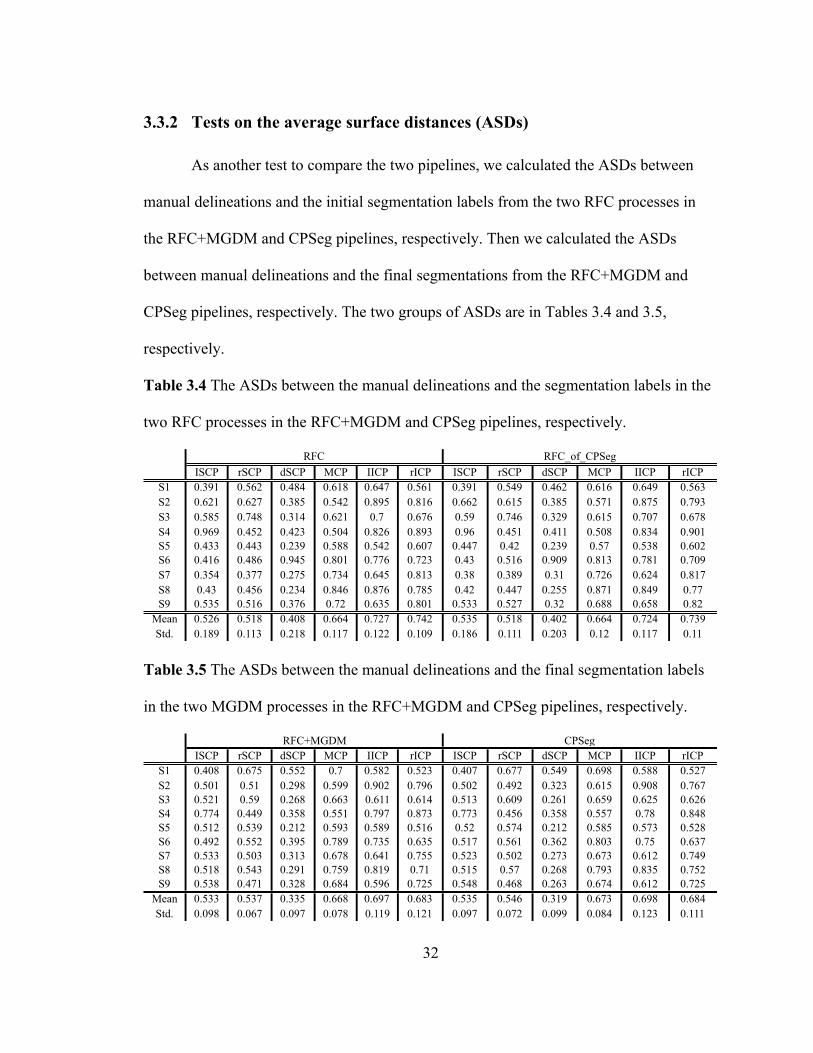
3.3.2 Tests on the average surface distances (ASDs)

As another test to compare the two pipelines, we calculated the ASDs between

manual delineations and the initial segmentation labels from the two RFC processes in

the RFC+MGDM and CPSeg pipelines, respectively. Then we calculated the ASDs

between manual delineations and the final segmentations from the RFC+MGDM and

CPSeg pipelines, respectively. The two groups of ASDs are in Tables 3.4 and 3.5,

respectively.

Table 3.4 The ASDs between the manual delineations and the segmentation labels in the

two RFC processes in the RFC+MGDM and CPSeg pipelines, respectively.


RFC RFC_of_CPSeg

Table 3.5 The ASDs between the manual delineations and the final segmentation labels

in the two MGDM processes in the RFC+MGDM and CPSeg pipelines, respectively.


RFC+MGDM CPSeg

33

To show the statistical significance of the segmentation differences between the

new and old pipelines, a paired Student’s t -test and a Wilcoxon signed-rank test were

performed with respect to ASDs. The p -values of the two tests are shown in Table 3.6.

Results show that the segmentation performances of the two pipelines are statistically the

same.


for comparing the ASDs between the RFC and RFC+MGDM results and the results from

CPSeg.

Paired Student’s t -test

ISCP rSCP dSCP MCP IICP rICP RFC 0.147 0.911 0.543 0.935 0.581 0.592

RFC+MGDM 0.546 0.145 0.107 0.377 0.827 0.855

Wilcoxon signed-rank test ISCP rSCP dSCP MCP IICP rICP

RFC 0.203 0.734 0.641 1 0.91 0.734 RFC+MGDM 1 0.164 0.109 0.57 1 0.734 Note: * p < 0.05

3.3.3 Conclusion

The paired Student’s t -test and the Wilcoxon signed-rank test with respect to the

Dice coefficients and the ASDs both show that the CPSeg and the RFC+MGDM are not

statistically different. The CPSeg performs even better than the RFC+MGDM on

segmenting the dSCPs. We can therefore use the CPSeg pipeline to process other datasets

and use these results as the basis of scientific conclusions.

34

Chapter 4 Outlier Detection on the

Tomacco Dataset

This chapter studies the performance of the automatic segmentation methods

described in Chapter 3 using the box-whisker plot, which implements a simple univariate

outlier detection method. Box plots display the lower extreme, lower quartile (25%),

median, upper quartile (75%), and upper extreme points of the data. Between the lower

and upper quartiles is the interquartile range (IQR), namely 50% of the data. Usually, a

data point is defined as an outlier when it is 1.5×IQR or more above the upper quartile, or

1.5×IQR or more below the lower quartile. This range can vary in different datasets.

The Tomacco datasets were processed using CATNAP-v1 for calculating

diffusion tensors and then using CPSeg for automatic segmentation of the CPs.

Additional information about this dataset is described in Chapter 3. We manually

categorized the automatic segmentations in the Tomacco dataset as a successful

segmentation or a segmentation failure. We then designed three kinds of features of the

image data from the categorized failures. Outliers were detected using the box-whisker

plot and they were considered as possible algorithm failure detections. We then evaluated

each feature’s performance based on the true positive and false positive rates.

4.1 Categorization of Automatic Segmentations

Successful and failed segmentations in our study were manually categorized by

36

We categorized all the segmentation labels of the 48 subjects in the Tomacco

dataset and assigned numerical scores to each subject for assessing the segmentation

quality. The Tomacco dataset’s information together with the categories and scores are

listed in Table 4.1. The “1” in this table means a segmentation failure while the “0”

means a successful segmentation. The numerical scores are integers ranging from 0 to 10.

Failed and successful segmentations are assigned scores ranging from 0–6 and 7–10

inclusively, respectively. Within the normal segmentations, there are some imperfect

ones with scores 7, 8, or 9. For example, segmentations with a small portion of the CPs

missing are considered as imperfect but successful. As shown in Table 4.1, among all the

Tomacco data, nine are categorized as segmentation failures and the rest are categorized

as successful segmentations. In the following section, we look into these failures to see

whether there are image features that can indicate potential segmentation failures.

37


gender, categories, and scores.

Number ID Diagnosis Gender Category Score Number ID Diagnosis Gender Category Score1 at1002 cb M 1 1 25 at1018 control F 0 102 at1103 control M 1 1 26 at1020 control F 0 103 at1016 cb M 1 4 27 at1021 control M 0 104 at1083 control F 1 4 28 at1022 cb F 0 105 at1034 SCA6 F 1 5 29 at1023 cb M 0 106 at1046 cb M 1 5 30 at1024 nph M 0 107 at1049 SCA6 F 1 5 31 at1025 cb F 0 108 at1007 cb F 1 5 32 at1026 control M 0 109 at1078 cb+ F 1 6 33 at1027 ?cb M 0 1010 at1081 control M 0 8 34 at1028 cb+ M 0 1011 at1032 control F 0 9 35 at1029 control F 0 1012 at1041 cb+ M 0 9 36 at1031 control F 0 1013 at1056 ?cb F 0 9 37 at1033 SCA6 F 0 1014 at1080 control F 0 9 38 at1036 cb+ F 0 1015 at1086 control M 0 9 39 at1038 vest M 0 1016 at1000 sca6 M 0 10 40 at1040 fam17/control M 0 1017 at1003 cb M 0 10 41 at1043 cb M 0 1018 at1005 fam17/cb F 0 10 42 at1044 control F 0 1019 at1006 cb M 0 10 43 at1045 control M 0 1020 at1011 cb F 0 10 44 at1048 SCA6 F 0 1021 at1013 ?cb M 0 10 45 at1060 cb M 0 1022 at1014 cb M 0 10 46 at1079 control F 0 1023 at1015 cb M 0 10 47 at1082 control F 0 1024 at1017 SCA6 M 0 10 48 at1084 control F 0 10

Note:LCategoryL1L:LsegmentationLfailure;LCategoryL0L:LsuccessfulLsegmentation

38

4.2 Feature Extraction

To design features for finding potential segmentation failures, we need to look

into the nine categorized failures in the Tomacco dataset first. Generally there are two

kinds of segmentation failures. The first kind is one with incomplete labels of the six

CPs. For example, some segmentation results only have three or four labels out of six.

Figures 4.2(b), (c), and (d) are three failures in this case. The labels for lSCP, rSCP and

dSCP are missing in segmentation results of subjects with IDs at1034 and at1049, shown

in Figures 4.2(b) and (c). The labels for dSCP and rICP are missing in the segmentation

result of the subject with ID at1083.

We define this kind of segmentation failure based on the assumption that every

person should have complete six labels. Subjects with ataxia may have relatively smaller

CPs, but the six structures should be complete. Maybe when the quality of the DTI scans

is poor, the smallest CP (dSCP) is not obvious in the linear Westin index for automatic

segmentation. Then the segmentation algorithm may fail to find it. This problem can

result from poor data quality rather than a flaw in the algorithm pipeline itself. Since we

are doing quality assurance on the whole pipeline including the raw datasets (DTI scans

and MPRAGE structural images), we consider this as a segmentation failure rather than a

successful segmentation. Obviously, whatever the reason for the missing labels, this kind

of segmentation results cannot be used for scientific analysis. Thus, given this

perspective, treating these kinds of segmentations as failures is reasonable.

The second kind of segmentation failure is one with abnormal shape, size, or

relative positions of the six CPs. In Figure 4.2, an image of a successful segmentation (for

39

reference) and nine images of nine segmentation failures of the Tomacco dataset are

shown in a similar anatomical position. In Figures 4.2(d) and (e), large portions of MCPs

are cut off. Figures 4.2(f)–(j) show failures with abnormal shapes of CPs.

In addition to the nine failures, there are also six imperfect segmentations in the

Tomacco dataset. Usually imperfect segmentations are those with a small missing portion

of a CP. For example, Figure 4.3 shows images where small portions of the MCP and

ICP have been cut out. By checking intermediate results in the whole pipeline

(CATNAP-v1 and CPseg), we found that the most likely source for the imperfect cases

lies in the brain masks, which were generated by a skull-stripping module in the

CATNAP-v1. Incomplete or asymmetric brain masks can cut off a portion of the CPs in

the Westin indices, which causes incomplete final segmentation images. Generally this is

not a big issue since, based on visual inspection, we found that the missing portions of

some CPs are very small that they can be ignored. However, if the degree of the

abnormality of a brain mask is too high, it can cut off a big portion of some CPs in a

segmentation result and make it a failure, which cannot be used for further scientific

analysis. For example, as shown in Figure 4.2(e), in a segmentation failure of a subject

with ID at1007, a large portion of the left brain mask is missing and this mask cuts off a

large portion of the left MCP.

42

Based on the analysis of the failed and imperfect segmentations above, three

kinds of features are designed. The first kind of feature is object oriented and

characterizes the failures on the peduncle level. The volumes and surface areas of CPs are

the two features in this category and computed directly from the segmentation labels,

notated as V = [v_ lSCP,v_ rSCP,v_ dSCP,v_MCP,v_ lICP,v_ rICP] and

S = [s_ lSCP, s_ rSCP, s_ dSCP, s_ lICP, s_ rICP] , respectively.

The second kind of feature is data quality oriented. Since the RFC is trained using

the linear Westin index (computed from the diffusion tensor) the tensor’s quality is

related to the segmentation quality directly. For example, the subjects in Figures 4.2(b),

(c), (i), and (j) have dim or abnormal linear Westin indices, which makes the structure of

the CPs very unclear. Thus, segmentation qualities of the four subjects are also greatly

affected. So we can conclude that the diffusion tensors and the failures are correlated.

Based on this observation, we chose some tensor related parameters as features. In

particular, we chose the means and standard deviations (SDs) of the fractional anisotropy

(FA), mean diffusivity (MD), and the three Westin indices of the whole brain,

respectively. The three features are notated as FA = [mean_FA, std _FA] ,

MD = [mean_MD, std _MD] , and

WI = [mean_Cl, std _Cl,mean_Cp, std _Cp,mean_Cs, std _Cs] , respectively. Cl ,Cp ,

and Cs are linear, planar and spherical Westin indices, respectively. Considering that the

linear Westin index of each peduncle is used train the RFC, to avoid its circular use, we

calculated all these parameters on the whole brain instead of just on the peduncles.

The third kind of feature is related to the brain masks. Analysis of segmentation

43

failures shows that abnormal brain masks can make the linear Westin index incomplete,

which may cut off some structures of the CPs. To find failures result from this reason, the

volume and symmetry of each subject’s brain mask are used as two features. We also

used the volumes of the two half brain masks as features, considering the incompleteness

of brain masks may occur in only onside, either right or left. The feature vector is

BM = [v_BM,v_ leftBM,v_ rightBM, sym] , where v_BM , v_ leftBM , and

v_ rightBM are volumes of a whole brain mask and its two halves, and

sym = v_ leftBM / v_ rightBM −1 is for representing the symmetry of a brain mask.

Generally, brain mask features are indirect and may not perform as well as other features

since failures resulting from this reason are relatively rare in the Tomacco dataset.

In summary, three kinds of features are used to try to detect segmentation failures.

The feature vector of a segmentation result is F = [V,S,FA,MD,WI,BM ] with a total of

26 numerical features.

4.3 Outlier Detection Results

We take the definition of an outlier from Grubbs (1969)—“An outlying

observation, or outlier, is one that appears to deviate markedly from other members of the

sample in which it occurs.” Outliers in our numerical data were detected using a box-

whisker plot. The bottom and top of the box are the first and third quartiles of the data.

Between them is the Interquartile Range (IQR), namely 50% of the data. If a data point is

1.5×IQR or more above the third quartile, or 1.5×IQR or more below the first quartile, it

is detected as an outlier. The notch in the boxplots displays a confidence interval around

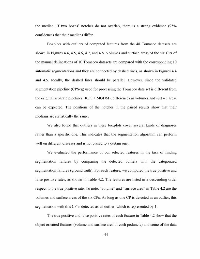
44

the median. If two boxes’ notches do not overlap, there is a strong evidence (95%

confidence) that their medians differ.

Boxplots with outliers of computed features from the 48 Tomacco datasets are

shown in Figures 4.4, 4.5, 4.6, 4.7, and 4.8. Volumes and surface areas of the six CPs of

the manual delineations of 10 Tomacco datasets are compared with the corresponding 10

automatic segmentations and they are connected by dashed lines, as shown in Figures 4.4

and 4.5. Ideally, the dashed lines should be parallel. However, since the validated

segmentation pipeline (CPSeg) used for processing the Tomacco data set is different from

the original separate pipelines (RFC + MGDM), differences in volumes and surface areas

can be expected. The positions of the notches in the paired results show that their

medians are statistically the same.

We also found that outliers in these boxplots cover several kinds of diagnoses

rather than a specific one. This indicates that the segmentation algorithm can perform

well on different diseases and is not biased to a certain one.

We evaluated the performance of our selected features in the task of finding

segmentation failures by comparing the detected outliers with the categorized

segmentation failures (ground truth). For each feature, we computed the true positive and

false positive rates, as shown in Table 4.2. The features are listed in a descending order

respect to the true positive rate. To note, “volume” and “surface area” in Table 4.2 are the

volumes and surface areas of the six CPs. As long as one CP is detected as an outlier, this

segmentation with this CP is detected as an outlier, which is represented by 1.

The true positive and false positive rates of each feature in Table 4.2 show that the

object oriented features (volume and surface area of each peduncle) and some of the data

45

quality related features (mean FA and the mean and standard deviation of the linear

Westin index) are generally perform better than the brain mask features. This is

consistent with our analysis on the brain mask features in Section 4.2. Among the data

quality features, mean MD does not perform well and we do not know the reason for this.

But at this time, it is too early to conclude that this feature is useless since Tomacco is a

relatively small dataset with limited segmentation failures. So MD is still used for outlier

detection in the following chapters.

Generally speaking, this univariate non-parametric outlier detection method using

boxplots can work on the Tomacco dataset. However, for assessing the performance of

the segmentation algorithm on a larger dataset and for detecting outliers more efficiently,

methods for multivariate outlier detection are needed. Before using more complex

methods, we will study a larger dataset in the next chapter using box-whisker plots to

double check the performance of these features.

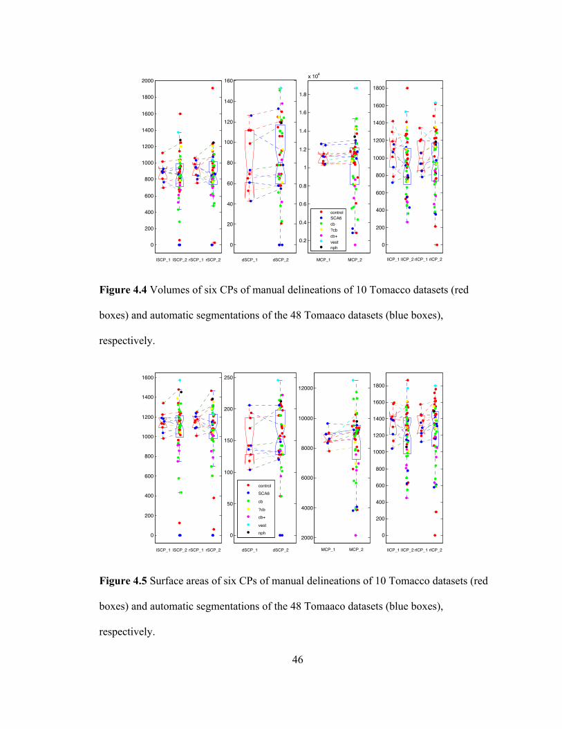
46

0

200

400

600

800

1000

1200

1400

1600

1800

2000

lSCP_1 lSCP_2 rSCP_1 rSCP_2

0

20

40

60

80

100

120

140

160

dSCP_1 dSCP_2

0.2

0.4

0.6

0.8

1

1.2

1.4

1.6

1.8

x 104

MCP_1 MCP_2

controlSCA6cb?cbcb+vestnph 0

200

400

600

800

1000

1200

1400

1600

1800

lICP_1 lICP_2 rICP_1 rICP_2

Figure 4.4 Volumes of six CPs of manual delineations of 10 Tomacco datasets (red


respectively.

0

200

400

600

800

1000

1200

1400

1600

lSCP_1 lSCP_2 rSCP_1 rSCP_2

0

50

100

150

200

250

dSCP_1 dSCP_2

2000

4000

6000

8000

10000

12000

MCP_1 MCP_2

control

SCA6

cb

?cb

cb+

vest

nph 0

200

400

600

800

1000

1200

1400

1600

1800

lICP_1 lICP_2 rICP_1 rICP_2

Figure 4.5 Surface areas of six CPs of manual delineations of 10 Tomacco datasets (red


respectively.

47

0.15

0.2

0.25

0.3

0.35

0.4

0.45

0.5

mean_FA

0.16

0.18

0.2

0.22

0.24

0.26

0.28

0.3

std_FA

1

1.1

1.2

1.3

1.4

1.5

1.6

x 10−3

mean_MD

5

6

7

8

9

10

11

12

13

x 10−4

std_MD

control SCA6 cb ?cb cb+ vest nph


datasets.

0.06

0.08

0.1

0.12

0.14

0.16

0.18

0.2

0.22

mean_cl

0.08

0.1

0.12

0.14

0.16

0.18

0.2

0.22

std_cl

0.1

0.12

0.14

0.16

0.18

0.2

0.22

0.24

0.26

0.28

0.3

mean_cp

0.12

0.14

0.16

0.18

0.2

0.22

0.24

0.26

0.28

std_cp

0.55

0.6

0.65

0.7

0.75

0.8

0.85

mean_cs

0.15

0.2

0.25

0.3

std_cs



Tomacco datasets.

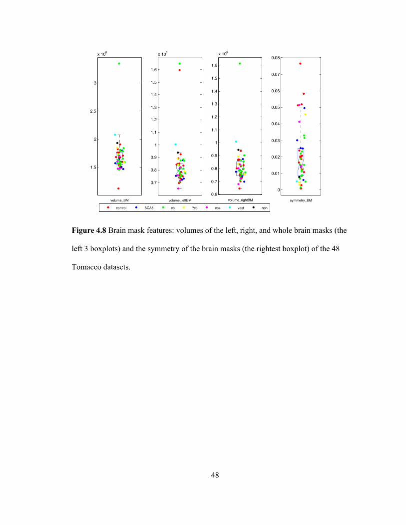
48

1.5

2

2.5

3

x 106

volume_BM

0.7

0.8

0.9

1

1.1

1.2

1.3

1.4

1.5

1.6

x 106

volume_leftBM

0.6

0.7

0.8

0.9

1

1.1

1.2

1.3

1.4

1.5

1.6

x 106

volume_rightBM

0

0.01

0.02

0.03

0.04

0.05

0.06

0.07

0.08

symmetry_BM


Figure 4.8 Brain mask features: volumes of the left, right, and whole brain masks (the

left 3 boxplots) and the symmetry of the brain masks (the rightest boxplot) of the 48

Tomacco datasets.

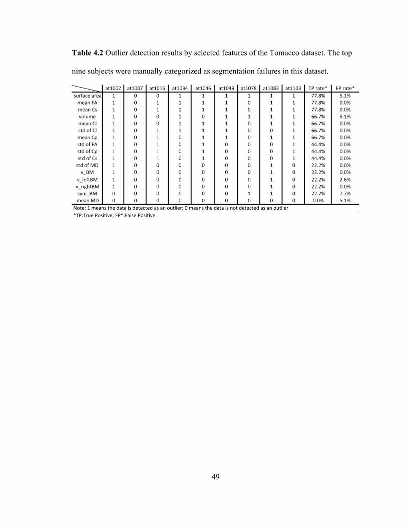
49

Table 4.2 Outlier detection results by selected features of the Tomacco dataset. The top

nine subjects were manually categorized as segmentation failures in this dataset.

at1002 at1007 at1016 at1034 at1046 at1049 at1078 at1083 at1103 TP.rate* FP.rate*surface.area 1 0 0 1 1 1 1 1 1 77.8% 5.1%mean.FA 1 0 1 1 1 1 0 1 1 77.8% 0.0%mean.Cs 1 0 1 1 1 1 0 1 1 77.8% 0.0%volume 1 0 0 1 0 1 1 1 1 66.7% 5.1%mean.Cl 1 0 0 1 1 1 0 1 1 66.7% 0.0%std.of.Cl 1 0 1 1 1 1 0 0 1 66.7% 0.0%mean.Cp 1 0 1 0 1 1 0 1 1 66.7% 0.0%std.of.FA 1 0 1 0 1 0 0 0 1 44.4% 0.0%std.of.Cp 1 0 1 0 1 0 0 0 1 44.4% 0.0%std.of.Cs 1 0 1 0 1 0 0 0 1 44.4% 0.0%std.of.MD 1 0 0 0 0 0 0 1 0 22.2% 0.0%v_BM 1 0 0 0 0 0 0 1 0 22.2% 0.0%

v_leftBM 1 0 0 0 0 0 0 1 0 22.2% 2.6%v_rightBM 1 0 0 0 0 0 0 1 0 22.2% 0.0%sym_BM 0 0 0 0 0 0 1 1 0 22.2% 7.7%mean.MD 0 0 0 0 0 0 0 0 0 0.0% 5.1%

Note:.1.means.the.data.is.detected.as.an.outlier;.0.means.the.data.is.not.detected.as.an.outlier*TP:True.Positive;.FP*:False.Positive

50

Chapter 5 Outlier Detection on the

Kwyjibo and Tomacco Datasets

This chapter studies the performance of the automatic segmentation methods

implemented with different CATNAPs on the Tomacco dataset and a larger dataset, the

Kwyjibo dataset, using box-whisker plots and supervised classification methods. The

Kwyjibo dataset, containing DTI and MPRAGE scans from 203 subjects: 49 healthy

controls and 154 patients with different kinds of ataxia, has the same type of data as the

Tomacco dataset since the DWIs of the two datasets were acquired using the same

sequence on the same 3T MR scanners (Intera, Philips Medical Systems, Netherlands).

Similar to the procedures on the Tomacco dataset, we first manually categorized all the

segmentation labels in the Kwyjibo dataset as successful segmentations and segmentation

failures. Then we processed Kwyjibo using CATNAP-v2 for estimating diffusion tensors

and using CPSeg for generating segmentation labels. Since CATNAP-v2 was used for

processing Kwyjibo data in the paper (Chuyang Ye et al., 2015), we used it rather than

the CATNAP-v1. Note that the Tomacco dataset was processed using CATNAP-v1,

which is slightly different from CATNAP-v2 on the parameter settings of two registration

modules and the versions of a skull-stripping module (called SPECTRE).

After the Kwyjibo dataset was processed, we found that some features, such as

surface area and MD, are statistically different from those of the Tomacco data processed

with CATNAP-v1. This is a problem since we want to merge the two datasets for further

51

study. To guarantee the validity of merging them, we reran the Tomacco data using

CATNAP-v2 and the CPSeg and verified the two CATNAP pipelines by quantitatively

comparing the volumes of the segmented CPs of the Tomacco dataset using the two

CATNAPs, respectively. Results show that the final segmentations using the two

CATNAP pipelines are different. Then by visually checking the segmentation results

processed by the two pipelines, we came to the conclusion that CATNAP-v2 performs

better than CATNAP-v1.

We next reassessed the performance of the automatic segmentation algorithm

using box-whisker plots on the reprocessed Tomacco data (using CATNAP-v2 and the

CPSeg). We found that the reprocessed Tomacco dataset has fewer segmentations

failures than the one using CATNAP-v1, which in turn further supports the conclusion

that CATNAP-v2 has a better performance.

Although the verification on the two CATNAP pipelines is not complete since we

did not compute Dice coefficients or ASDs, it at least provided some supporting evidence

for the conclusion above. (Note that Dice coefficients and ASDs were not compared

because the two algorithms use different digital grid sizes and therefore these comparison

metrics are not directly computable.) Thus, it is sensible to use CATNAP-v2 for

processing both the Tomacco and Kwyjibo data. In the next section, we merge them

together for using supervised classification methods on outlier detection.

Last, we combined the reprocessed Tomacco dataset and the Kwybjio dataset

together and used four supervised classifiers—linear discriminant analysis (LDA),

logistic regression (LR), support vector machine (SVM), and random forest classifier

(RFC). All categorized segmentation failures in the two datasets were used for training

52

these classifiers. Their performances were validated using a leave-one-out cross-

validation.

5.1 Categorization of Automatic Segmentations

Kwyjibo is a dataset containing DTI and MPRAGE scans from 203 subjects: 49

healthy controls and 154 patients with different kinds of ataxia. Some patients were

scanned more than once. This dataset can be processed the same as that of Tomacco since

the DWIs of the two datasets were acquired using the same sequence on the same 3T MR

scanners (Intera, Philips Medical Systems, Netherlands). However, there are two key

differences between the two datasets: 1) the population of subjects with ataxia is much

larger in the Kwyjibo dataset than that in the Tomacco dataset and 2) The MPRAGE

scans in the Tomacco dataset were registered to MNI space and have a 1mm isotropic

resolution while MPRAGE cans in the Kwyjibo dataset were not registered to MNI space

and have a 0.828mm isotropic resolution. Thus, the inputs (MPRAGE scans) to the two

CATNAPs have different resolutions.

To evaluate the performance of selected features to identify failed segmentations

in the Kwyjibo dataset, we first manually categorized segmentation results in the

Kwyjibo dataset as a segmentation failure or a successful segmentation in the same way

for Tomacco. Given extensive experience on the Tomacco data, it only took around three

days to categorize all the 203 datasets in Kwyjibo. The category, numerical scores for

segmentation quality, diagnosis, and gender information of eight failures and two

imperfect segmentations of the Kwyjibo data are presented in Table 5.1. Because this

dataset is relatively large, we only listed the segmentations with scores lower than 10.

53

The remaining datasets not listed here are given the full score 10 as they are successful

segmentations. We found eight segmentations failures and two imperfect but successful

segmentations in the Kwyjibo dataset, as shown in Table 5.1. The images and

descriptions of the eight segmentation failures are shown in Figure 5.1.

54

Table 5.1 Information of the categorized segmentation failures and imperfect but

successful segmentations in the Kwyjibo dataset including ID, diagnoses, gender,

categories, and scores.

Number ID Diagnosis Gender Category Score1 AT1219_20100730 axatia M 1 12 AT1556_20110802 SCA2 F 1 13 AT1275_20070402 ATF M 1 54 AT1061_20080804 MSA F 1 55 AT1061_20090306 MSA F 1 56 AT1532_20091202 sporadicFataxia F 1 67 AT1569_20101001 friedrich'sFataxia M 1 68 AT1594_20121129 SCA1 M 1 69 AT1313_20080315 controlF M 0 910 AT1315_20080324 control M 0 9

Note:FCategoryF1F:FsegmentationFfailure;FCategoryF0F:FsuccessfulFsegmentation

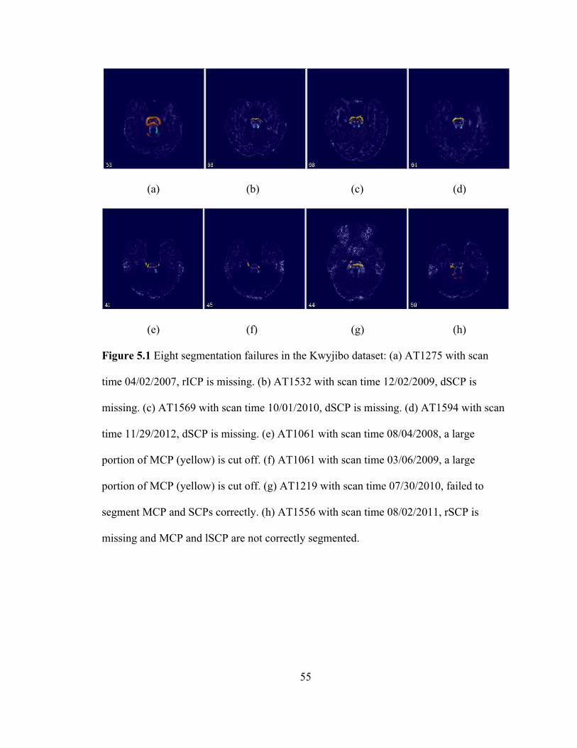
56

5.2 Outlier Detection Results

We used the outlier detection method on the Kwyjibo dataset in the same way as

before. Outliers detected by features (volumes and surface areas of the CPs, means and

standard deviations of the FA, MD, and three Westin indices, and the brain mask

features) on the Kwyjibo dataset are shown in Figures 5.2, 5.3, 5.4, 5.5, and 5.6. The

detected outliers in the Tomacco dataset by these features are also included in the

boxplots for comparison the data distributions of the two datasets. The outlier detection

results and true positive and false positive rates of these features are summarized in Table

5.2.

In Table 5.2, we observe that some features, which can robustly detect true

segmentation failures on the Tomacco dataset, do not work effectively on the Kwyjibo

dataset. For example, except for the spherical Westin index, all the remaining features

belonging to data quality oriented features failed to detect any true segmentation failure

by outlier detection. As well, the three brain mask features (the volumes of the right, left,

and the whole brain mask) also failed to detect true segmentation failures.

The inferior performance of these features on the Kwyjibo dataset is not our

expectation. However, by looking into the segmentation failures and imperfect but

successful segmentations in both the Tomacco and Kwyjibo datasets, we believe that the

poor performances of the features on the Kwyjibo dataset is explainable and reasonable.

In total there are eight segmentation failures and two imperfect segmentations in the 203

Kwyjibo datasets, while there are nine segmentation failures and six imperfect

segmentations in the 48 Tomacco datasets by visual inspection. The percentage of

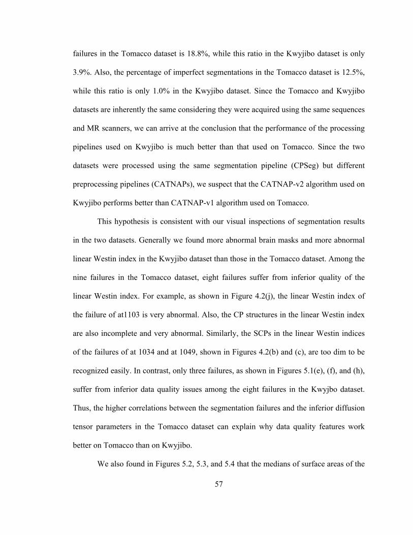
57

failures in the Tomacco dataset is 18.8%, while this ratio in the Kwyjibo dataset is only

3.9%. Also, the percentage of imperfect segmentations in the Tomacco dataset is 12.5%,

while this ratio is only 1.0% in the Kwyjibo dataset. Since the Tomacco and Kwyjibo

datasets are inherently the same considering they were acquired using the same sequences

and MR scanners, we can arrive at the conclusion that the performance of the processing

pipelines used on Kwyjibo is much better than that used on Tomacco. Since the two

datasets were processed using the same segmentation pipeline (CPSeg) but different

preprocessing pipelines (CATNAPs), we suspect that the CATNAP-v2 algorithm used on

Kwyjibo performs better than CATNAP-v1 algorithm used on Tomacco.

This hypothesis is consistent with our visual inspections of segmentation results

in the two datasets. Generally we found more abnormal brain masks and more abnormal

linear Westin index in the Kwyjibo dataset than those in the Tomacco dataset. Among the

nine failures in the Tomacco dataset, eight failures suffer from inferior quality of the

linear Westin index. For example, as shown in Figure 4.2(j), the linear Westin index of

the failure of at1103 is very abnormal. Also, the CP structures in the linear Westin index

are also incomplete and very abnormal. Similarly, the SCPs in the linear Westin indices

of the failures of at 1034 and at 1049, shown in Figures 4.2(b) and (c), are too dim to be

recognized easily. In contrast, only three failures, as shown in Figures 5.1(e), (f), and (h),

suffer from inferior data quality issues among the eight failures in the Kwyjbo dataset.

Thus, the higher correlations between the segmentation failures and the inferior diffusion

tensor parameters in the Tomacco dataset can explain why data quality features work

better on Tomacco than on Kwyjibo.

We also found in Figures 5.2, 5.3, and 5.4 that the medians of surface areas of the

58

CPs, the means and standard deviations of the MD, and the means and standard

deviations of the three Westin indices are statistically different between the Tomacco and

Kwyjibo datasets with a significance level 0.05. The medians of the other features

between the two datasets are statistically the same with the same significance level. This

is not what we expected since we have assumed that the calculated features on the two

datasets are comparable. Since the categories and populations of the neurological

diagnosis influencing the cerebellar peduncles between the two datasets are different, the

differences in features of the MD and Westin indices may be sensible. However, the

significant differences in surface areas of the CPs between the two datasets cannot be

explained since the corresponding volumes of the CPs are statistically the same. As we

mentioned before, we used CATNAP-v2 on Kwyjibo because it was used on Kwyjibo in

Ye et al. (2015). Thus, given the preceding observations, to guarantee the validity of

merging Tomacco and Kwyjibo together, we should reprocess the Tomacco dataset using

CATNAP-v2.

Before the CATNAP-v2 algorithm can be adopted formally for the Tomacco

dataset, we must verify it. In next section, we verify the CATNAP-v2 quantitatively and

qualitatively.

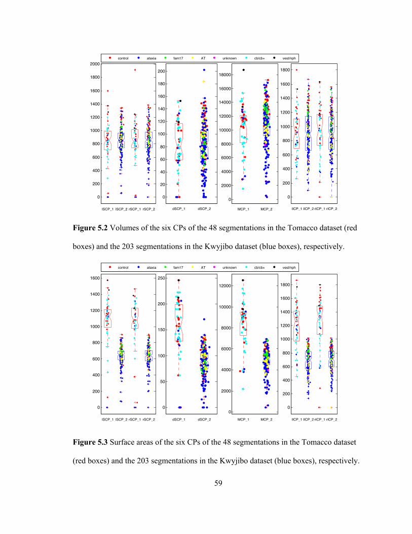
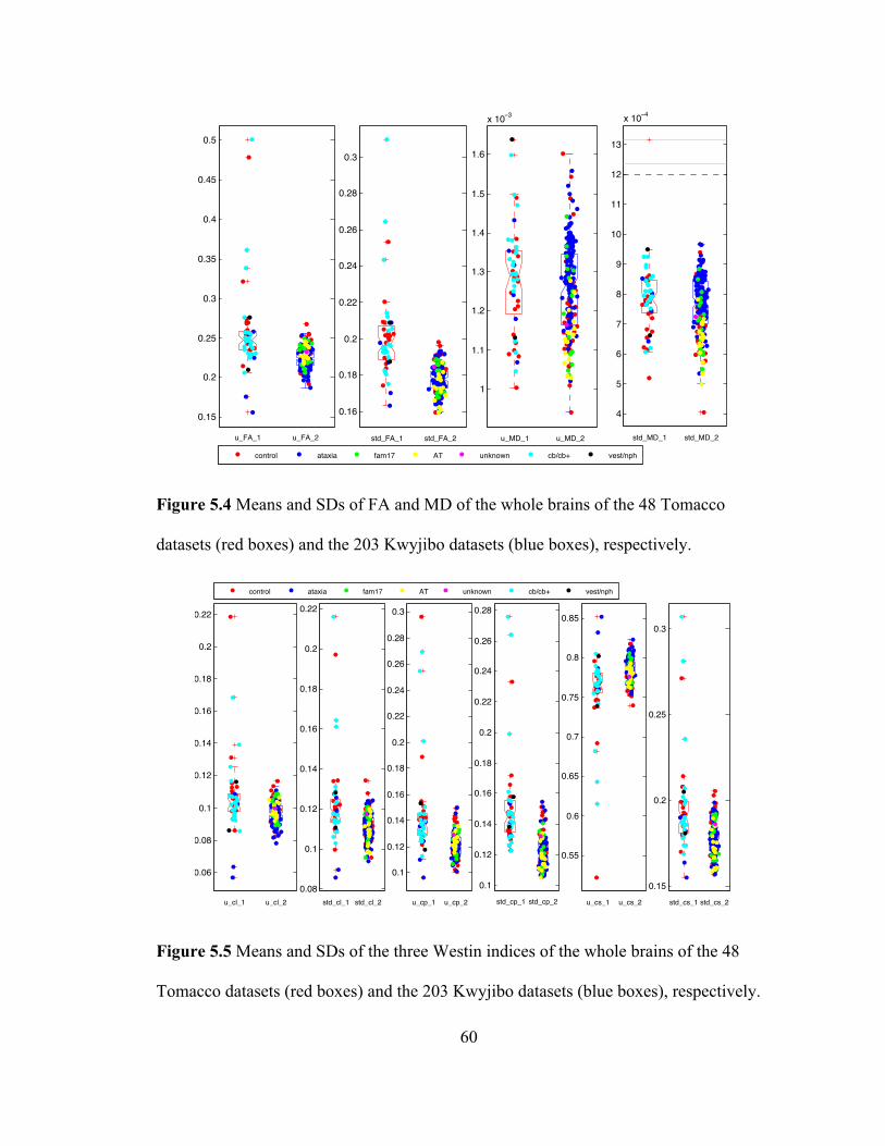
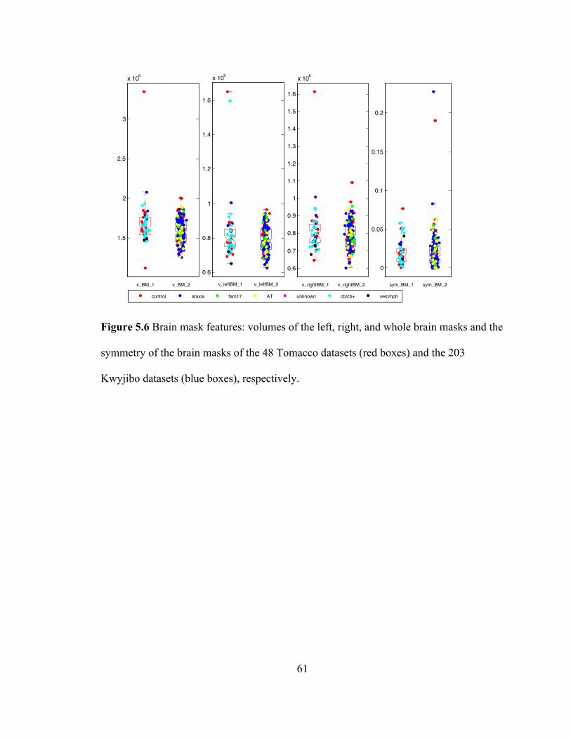
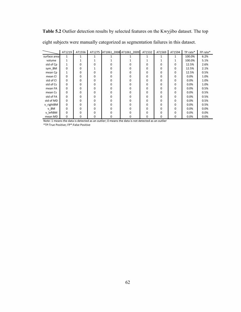
62

Table 5.2 Outlier detection results by selected features on the Kwyjibo dataset. The top

eight subjects were manually categorized as segmentation failures in this dataset.

AT1219 AT1556 AT1275 AT1061_2008 AT1061_2009 AT1532 AT1569 AT1594 TP/rate* FP/rate*surface/area 1 1 1 1 1 1 1 1 100.0% 6.2%volume 1 1 1 1 1 1 1 1 100.0% 5.1%std/of/Cp 1 0 0 0 0 0 0 0 12.5% 2.6%sym_BM 0 0 1 0 0 0 0 0 12.5% 2.1%mean/Cp 1 0 0 0 0 0 0 0 12.5% 0.5%mean/Cl 0 0 0 0 0 0 0 0 0.0% 1.0%std/of/Cl 0 0 0 0 0 0 0 0 0.0% 1.0%std/of/Cs 0 0 0 0 0 0 0 0 0.0% 1.0%mean/FA 0 0 0 0 0 0 0 0 0.0% 0.5%mean/Cs 0 0 0 0 0 0 0 0 0.0% 0.5%std/of/FA 0 0 0 0 0 0 0 0 0.0% 0.5%std/of/MD 0 0 0 0 0 0 0 0 0.0% 0.5%v_rightBM 0 0 0 0 0 0 0 0 0.0% 0.5%v_BM 0 0 0 0 0 0 0 0 0.0% 0.0%

v_leftBM 0 0 0 0 0 0 0 0 0.0% 0.0%mean/MD 0 0 0 0 0 0 0 0 0.0% 0.0%Note:/1/means/the/data/is/detected/as/an/outlier;/0/means/the/data/is/not/detected/as/an/outlier*TP:True/Positive;/FP*:False/Positive

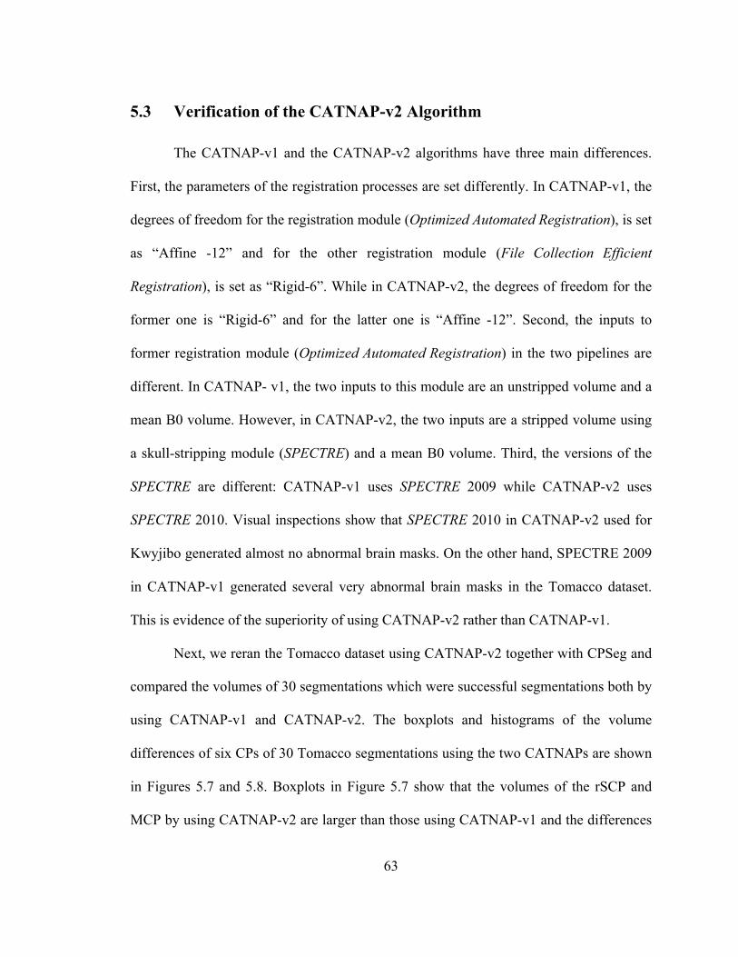
63

5.3 Verification of the CATNAP-v2 Algorithm

The CATNAP-v1 and the CATNAP-v2 algorithms have three main differences.

First, the parameters of the registration processes are set differently. In CATNAP-v1, the

degrees of freedom for the registration module (Optimized Automated Registration), is set

as “Affine -12” and for the other registration module (File Collection Efficient

Registration), is set as “Rigid-6”. While in CATNAP-v2, the degrees of freedom for the

former one is “Rigid-6” and for the latter one is “Affine -12”. Second, the inputs to

former registration module (Optimized Automated Registration) in the two pipelines are

different. In CATNAP- v1, the two inputs to this module are an unstripped volume and a

mean B0 volume. However, in CATNAP-v2, the two inputs are a stripped volume using

a skull-stripping module (SPECTRE) and a mean B0 volume. Third, the versions of the

SPECTRE are different: CATNAP-v1 uses SPECTRE 2009 while CATNAP-v2 uses

SPECTRE 2010. Visual inspections show that SPECTRE 2010 in CATNAP-v2 used for

Kwyjibo generated almost no abnormal brain masks. On the other hand, SPECTRE 2009

in CATNAP-v1 generated several very abnormal brain masks in the Tomacco dataset.

This is evidence of the superiority of using CATNAP-v2 rather than CATNAP-v1.

Next, we reran the Tomacco dataset using CATNAP-v2 together with CPSeg and

compared the volumes of 30 segmentations which were successful segmentations both by

using CATNAP-v1 and CATNAP-v2. The boxplots and histograms of the volume

differences of six CPs of 30 Tomacco segmentations using the two CATNAPs are shown

in Figures 5.7 and 5.8. Boxplots in Figure 5.7 show that the volumes of the rSCP and

MCP by using CATNAP-v2 are larger than those using CATNAP-v1 and the differences

64

are statistically significant since the notches do not overlap with zero. The volumes of the

other four CPs by using the two CATNAPs are statistically the same.

Next we visually checked the segmentation results using the two CATNAPs. We

first resampled the Tomacco segmentations (from CATNAP-v1) from the original 1mm

isotropic resolution to a 0.828mm isotropic grid. Then we registered the resampled

segmentations to the corresponding segmentations using CATNAP-v2 with a 0.828mm

isotropic resolution. Then we subtracted the registered segmentations to the

segmentations using CATNAP-v2 and overlaid the subtracted image onto the

corresponding MPRAGE images. Compared with some MCPs in the segmentations

results using CATNAP-v1, we found that those using CATNAP-v2 are more similar to

the MCPs in MPRAGE images, as shown in Figure 5.9.

In summary, segmentation results using the two CATNAPs are statistically

different. There were fewer abnormal brain masks in the Kwyjibo data using CATNAP-

v2 and more accurate segmented MCPs in the reprocessed Tomacco data using

CATNAP-v2 compared with those using CATNAP-v1. Thus we believe that CATNAP-

v2 performs better than CATNAP-v1 and decided to continue use of CATNAP-v2.

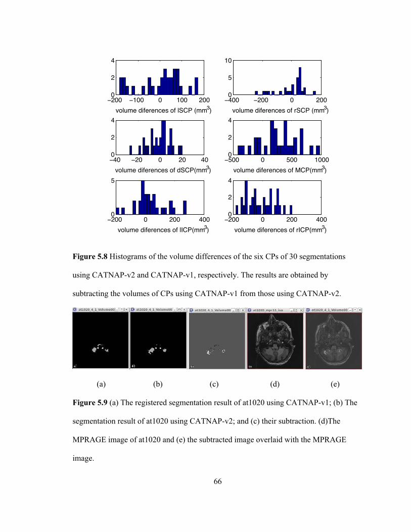
67

5.4 Reproduction of the Tomacco Dataset

In order to merge the Tomacco and Kwyjibo datasets, we reran the Tomacco

dataset using the CATNAP-v2 and the CPSeg (exactly the same pipelines used on the

Kwyjibo dataset). We then studied the performance of the automatic segmentation

algorithm on the reprocessed Tomacco dataset in the same way as we did on the Kwyjibo

dataset.

First we categorized the segmentations from the reprocessed Tomacco data as

segmentation failures or successful segmentations. Because of quality issues of their

MRPAGE images, we excluded two subjects (at1081 and at 1083) from the 48 Tomacco

data. Therefore, we reprocessed only 46 Tomacco datasets in this study. As shown in

Table 5.3, we found a total of four segmentation failures among the 46 Tomacco data.

Since they were previously shown in Figures 4.2(b), (c), (i), and (j) in Chapter 4, we do

not show images of them here.

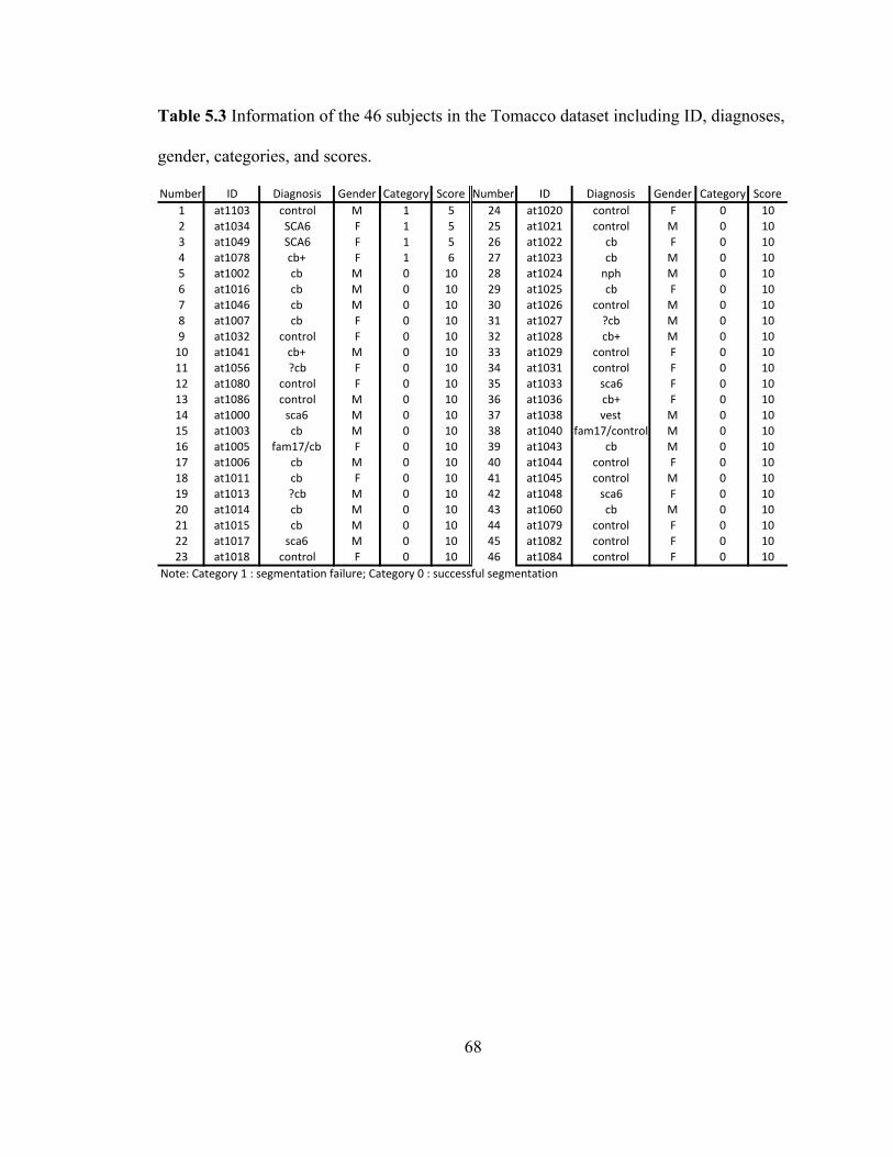
68


gender, categories, and scores.

Number ID Diagnosis Gender Category Score Number ID Diagnosis Gender Category Score1 at1103 control M 1 5 24 at1020 control F 0 102 at1034 SCA6 F 1 5 25 at1021 control M 0 103 at1049 SCA6 F 1 5 26 at1022 cb F 0 104 at1078 cb+ F 1 6 27 at1023 cb M 0 105 at1002 cb M 0 10 28 at1024 nph M 0 106 at1016 cb M 0 10 29 at1025 cb F 0 107 at1046 cb M 0 10 30 at1026 control M 0 108 at1007 cb F 0 10 31 at1027 ?cb M 0 109 at1032 control F 0 10 32 at1028 cb+ M 0 1010 at1041 cb+ M 0 10 33 at1029 control F 0 1011 at1056 ?cb F 0 10 34 at1031 control F 0 1012 at1080 control F 0 10 35 at1033 sca6 F 0 1013 at1086 control M 0 10 36 at1036 cb+ F 0 1014 at1000 sca6 M 0 10 37 at1038 vest M 0 1015 at1003 cb M 0 10 38 at1040 fam17/control M 0 1016 at1005 fam17/cb F 0 10 39 at1043 cb M 0 1017 at1006 cb M 0 10 40 at1044 control F 0 1018 at1011 cb F 0 10 41 at1045 control M 0 1019 at1013 ?cb M 0 10 42 at1048 sca6 F 0 1020 at1014 cb M 0 10 43 at1060 cb M 0 1021 at1015 cb M 0 10 44 at1079 control F 0 1022 at1017 sca6 M 0 10 45 at1082 control F 0 1023 at1018 control F 0 10 46 at1084 control F 0 10

Note:LCategoryL1L:LsegmentationLfailure;LCategoryL0L:LsuccessfulLsegmentation

69

By using boxplots, outliers were detected in the 46 Tomacco datasets. The

boxplots with detected outliers are shown in Figures 5.10, 5.11, 5.12, 5.13, and 5.14 and

the outlier detection results are shown in Table 5.3. Consistent with the feature

performance results on the 48 Tomacco data using CATNAP-v1, the object features and

the data quality features work well on the 46 reprocessed Tomacco datasets except for the

mean and standard deviation of the MD. The brain mask features perform worse than the

other two kinds of features, which is also consistent with the previous results that used

CATNAP-v1 in the 48 Tomacco datasets.

Since the Tomacco datasets were reprocessed using the same pipeline as Kwyjibo,

we can merge them together for a new outlier detection study. With the manual

categorization of all the segmentation results on both datasets (as either successful or

failed), several supervised classification methods for outlier detection are used to develop

an automatic method to detect successful or failed segmentations. Details are described in

the next section.

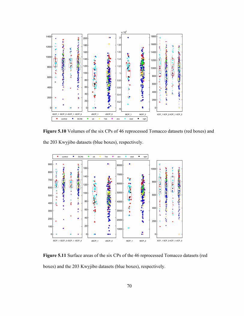
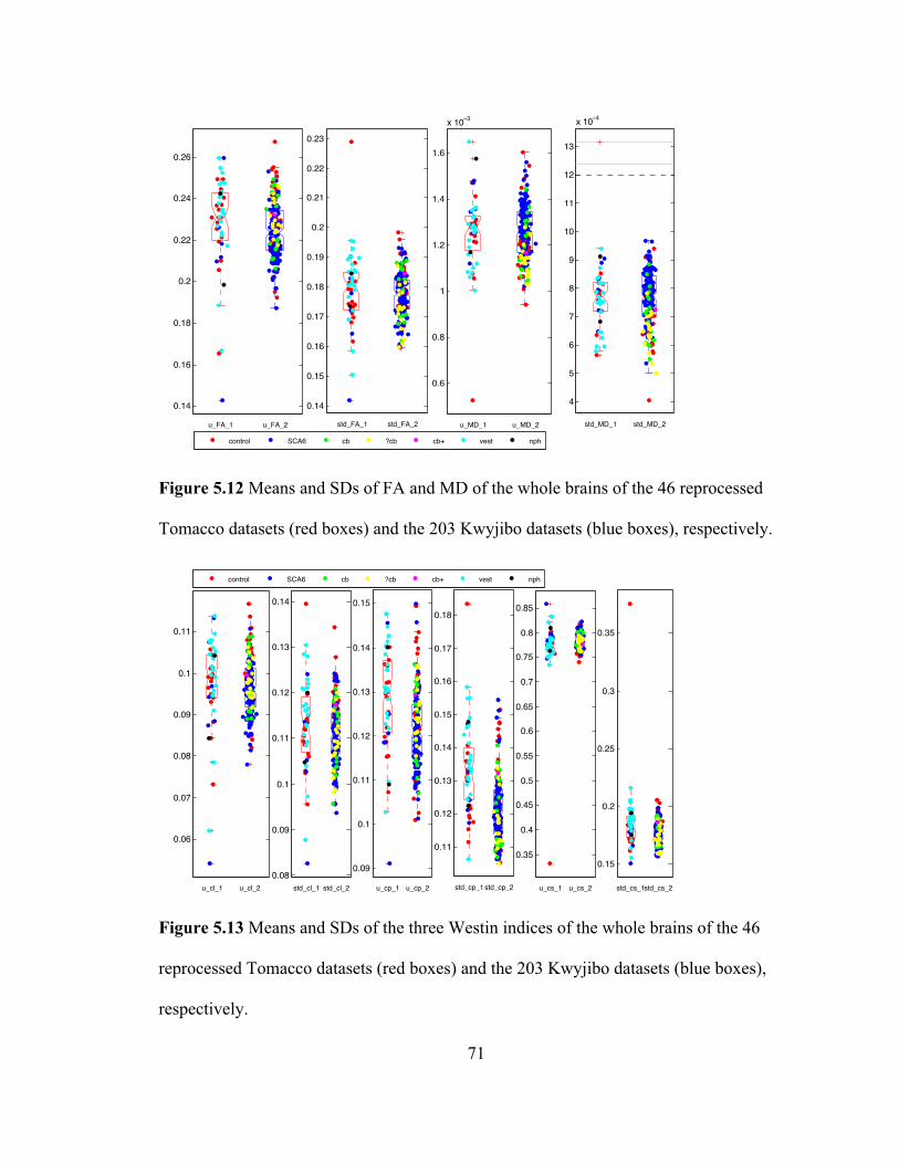
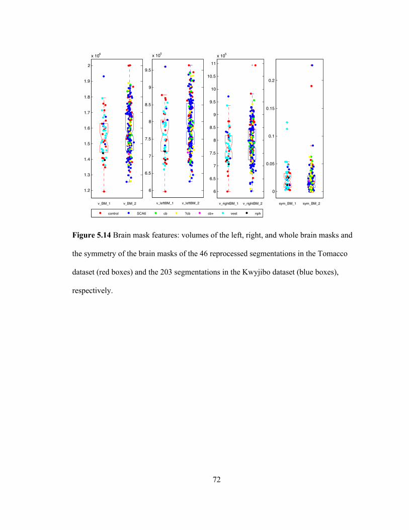
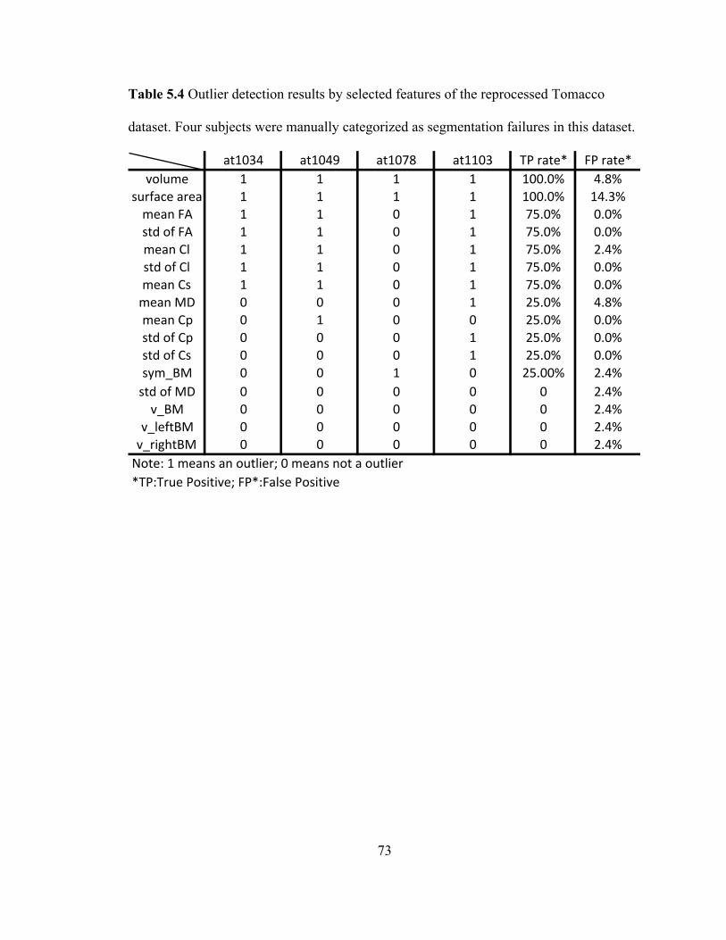
73

Table 5.4 Outlier detection results by selected features of the reprocessed Tomacco

dataset. Four subjects were manually categorized as segmentation failures in this dataset.

at1034 at1049 at1078 at1103 TP,rate* FP,rate*volume 1 1 1 1 100.0% 4.8%

surface,area 1 1 1 1 100.0% 14.3%mean,FA 1 1 0 1 75.0% 0.0%std,of,FA 1 1 0 1 75.0% 0.0%mean,Cl 1 1 0 1 75.0% 2.4%std,of,Cl 1 1 0 1 75.0% 0.0%mean,Cs 1 1 0 1 75.0% 0.0%mean,MD 0 0 0 1 25.0% 4.8%mean,Cp 0 1 0 0 25.0% 0.0%std,of,Cp 0 0 0 1 25.0% 0.0%std,of,Cs 0 0 0 1 25.0% 0.0%sym_BM 0 0 1 0 25.00% 2.4%std,of,MD 0 0 0 0 0 2.4%v_BM 0 0 0 0 0 2.4%

v_leftBM 0 0 0 0 0 2.4%v_rightBM 0 0 0 0 0 2.4%Note:,1,means,an,outlier;,0,means,not,a,outlier*TP:True,Positive;,FP*:False,Positive

74

5.5 Outlier Detection using Classification Methods

In this section, we use supervised learning methods, as described in Chapter 2, to

develop classifier for detection of failed segmentations. With the manual categorization

(into success or failure) of the 46 Tomacco datasets (yielding four segmentation failures

and 42 successful segmentations) and the 203 Kwyjibo datasets (yielding eight

segmentation failures and 195 successful segmentations), we are able to train classifiers

for automatically failure detection. Considering the limited quantities of the segmentation

failures in both datasets, we decided to combine them together and use all the 12 failures

for training. We trained four binary classifiers—linear discriminant analysis (LDA),

logistic regression (LR), support vector machine (SVM), and random forest classifier

(RFC). The performances of the four classifiers were evaluated using a leave-one-out

cross-validation. Details are presented in the next sections.

5.5.1 The four classifiers

LDA is a method used in statistics, pattern recognition, and machine learning to

find a linear combination of features that separate two or more classes. Logistic

regression is similar to LDA. We used it for comparison with LDA.

SVM is a supervised learning model in machine learning for classification and

regression analysis. It can generate classifiers from poorly balanced data, which is often

the case in medical domains where abnormal data is rare or difficult to obtain. In SVMs,

the input data is projected to higher dimensional space by a kernel function to find a

hyperplane that distinguishes normal data and outliers. The kernel can be a linear dot

75

product, a polynomial function, a radial basis function, or a sigmoid function. We

adopted the linear dot product kernel since it performed best among the four kinds of

kernels based on our trial experiments.

Random forest classifier, an ensemble classification method, is a collection of

decisions trees that usually performs better than a single decision tree. It was introduced

detail in Chapter 2. No more additional description is provided here. We used 100 trees in

implementing this classifier and averaged the misclassification rate, true positive rate,

and false positive over 20 runs.

5.5.2 Training sets

To train the classifiers, we must select a representative training set. Choosing a

proper training set is very critical since it directly affects the generalization and

classification accuracy of the classifiers. In our datasets, we have only four segmentation

failures in the Tomacco dataset and eight segmentation failures in the Kwyjibo dataset.

To provide the most information about failures in training, we used all 12 segmentation

failures in our training sets. Since failure detection is a binary classification task, we must

also include successful segmentations in the training set. There are a total of 237

successful segmentations in the two datasets. We built two training sets to evaluate. The

first one consists of 12 segmentation failures and all of the 237 successful segmentations.

The second one consists of 12 segmentation failures and only 24 randomly selected

successful segmentations among the 237 segmentations.

The features we used are the same as before: the object features, the data quality

features, and the brain masks features. The feature vector is F = [V,S,FA,MD,WI,BM ] ,

76

where V and S are the object features (volumes and surface areas of the six CPs), FA,

MD, and WI are the data quality features (means and standard deviations of FA, MD, and

the three Westin indices, respectively), and BM are the brain masks features (the volumes

of the left, right, and whole brain masks as well as the symmetry of the brain masks). A

total of 26 numerical features are used. Considering the range of volumes and surface

areas are much larger than that of the data quality oriented features, we normalized all the

feature values before training the classifiers. For each feature, the normalization was

performed by subtracting the mean of the feature values from each data and then dividing

the standard deviation of the feature values.

5.5.3 Performance evaluation

We evaluated the four classifiers using leave-one-out cross-validation on each of

the two training sets. When a subject of one training set was tested (the segmentation

result), the remaining subjects in this set were used in the training phase (which means,

for example, that when a failure is being evaluated only 11 failures are used in the

training set). The misclassification rate (MCR), true positive (TP) and false positive (FP)

rates as well as the numbers of true and false positives on both training sets are shown in

Table 5.5.

Table 5.5 shows that in the first (larger) training set, the RFC performs best and

the LR performs worst among the four classifiers. The performances of the LDA and the

linear SVM are very similar. In the second training set, the LDA, the LR, and the linear

SVM perform similarly and the RFC’s performance is just a little bit worse than other

three. Considering that the second training set only contains 24 randomly selected

77

successful segmentations, the inferior performance of RFC on this training set is not

surprising. It is hard to come to a conclusion about which classifier performs best. Taking

both performances on the two training sets, the total numbers of true positives and false

positives are 19 and 4 using LDA, 18 and 7 using LR, 17 and 2 using SVM, and 19 and 3

using RFC, respectively. In summary, the LR performs worst among the four classifiers

and the other three perform comparably.

78

Table 5.5 Performance comparison of the four classifiers (LDA, LR, SVM, and RFC) on

the combined Tomacco and Kwyjibo dataset.

MCR # TP # FP TP rate FP rateLDA 0.028 8 3 0.667 0.013LR 0.044 7 6 0.583 0.025

SVM(linear) 0.028 7 2 0.583 0.008RFC* 0.021(0.002) 9 2 0.75(0) 0.009(0.002)

MCR # TP # FP TP rate FP rateLDA 0.056 11 1 0.917 0.042LR 0.056 11 1 0.917 0.042

SVM(linear) 0.056 10 0 0.833 0RFC* 0.075(0.013) 10 1 0.863(0.041) 0.044(0.009)

* 100 trees, mtry = 4, average on 20 runs

Training set 1

Training set 2

79

Chapter 6 Conclusions and Future Work

In this thesis, we presented an approach to quality assurance using outlier

detection for the automatic cerebellar peduncle segmentation algorithm presented by Ye.

et al. (Chuyang Ye et al., 2015). In this chapter, we summarize the main contributions of

this thesis and suggest future improvements.

6.1 Main Contributions

Three main contributions are made in this thesis. First, we validated a new

cerebellar peduncle segmentation pipeline (CPSeg) against the corresponding old

pipeline (RFC+MGDM) which was used in the paper reporting the peduncle

segmentation algorithm. Dice coefficients (Dice, 1945) and average surface distances

(ASDs) between nine segmentation results and corresponding manual delineations were

computed on both pipelines. A paired Student’s t -test and a Wilcoxon signed-rank test

(significance level 0.05) were performed with respect to the Dice coefficients and the

ASDs, respectively. Testing results on the Dice coefficients and the ASDs show that the

performance between the CPSeg and the RFC+MGDM are not statistically different.

Furthermore, results of the two tests on the Dice coefficients indicate that the CPSeg

segments the dSCP better.

Second, we validated a preprocessing pipeline, CATNAP, against a slightly

different version of this pipeline. We call the old version CATNAP-v1 and the new

version CATNAP-v2. This validation was necessary since the Tomacco and Kwyjibo

80

datasets were processed using different CATNAP versions, but we wanted to combine

them for outlier detection using supervised classification. We conducted both quantitative

and visual inspection of the segmentation results in the Tomacco dataset using the two

CATNAPs as the preprocessing step. Results show that the CATNAP-v2 generates

statistically different volumes of the MCPs compared with that of CATNAP-v1. Visual

inspection of the segmentation results shows that CATNAP-v2 performs slightly better

on segmenting the MCPs.

Third, we studied the performance of the automatic segmentation algorithm using

box-whisker plots and four supervised classifiers for failure detection. We first manually

categorized the segmentation results in the Tomacco dataset as a segmentation failure or

a successful segmentation. We then designed three kinds of features of the image data

from the categorized failures in the Tomacco dataset for detecting potential segmentation

failures automatically. With these features, we detected outliers using boxplots and

evaluated each feature’s performance. Next, we did a similar outlier detection study using

box-whisker plots on the Kwyjibo dataset with 203 subjects. This dataset only has eight

segmentation failures and two imperfect but successful segmentations. Then we

reprocessed the Tomacco dataset using the same algorithm pipeline as used for Kwyjibo

and merged the two datasets together. With the manually categorized segmentation

results as training data, we detected failures automatically by using four classifiers—

linear discriminant analysis (LDA), logistic regression (LR), support vector machine

(SVM), and random forest classifier (RFC). We evaluated the performance of each

classifier using a leave-one-out cross-validation and computed the true positives and false

positives of each classifier. Our results show that the performances of the LDA, the linear

81

SVM and the RFC are not very different and LR performs worse than the other three

classifiers.

6.2 Future Work

In sum, this project can be best described as an exploration on quality assurance

for the performance of the automatic segmentation algorithm using outlier detection. For

example, before looking into the segmentation failures, we did not have a clear mind

about the quantity, appearance, and the reasons why they became failures. Thus we did

not plan to use classification methods for outlier detection until we had enough

information about the failures in the two datasets. So the work in this project is just a

small starting point on quality assurance using outlier detection for the proposed

segmentation algorithm. Many improvements should be done in the future.

First, more effective features to improve the classification accuracy and

distinguish the outlier failures and naturally occurring derivations should be extracted.

Features for registration accuracy and correctness and the quality of the PEVs in the

CPSeg pipeline can be considered in the future. Furthermore, the data quality features

such as the means and standard deviations of FA, the MD, and the three Westin indices of

the whole brain do not perform as well as the object features like the volumes and surface

areas of the CPs. How to modify these features and make them more effective remains to

be studied. As well, although volumes and surface areas of the CPs can effectively detect

true segmentation failures, the false positive rates of them are also relatively higher than

other features since there are naturally occurring subjects with extreme volumes.

Boxplots and the supervised classifiers cannot necessarily distinguish extreme

82

data/anatomy from algorithm failures. If alterative features can be developed to replace

the two object features, this problem may be solved.

Second, since there are a total of 12 segmentation failures in the combined

Tomacco and Kwyjibo dataset, the generalization of the four classifiers trained on the

two datasets needs to be further studied. Therefore, we probably should apply these

classifiers on other separate datasets with other diagnoses to evaluate their accuracies.

Lastly, the general approach that we have pursued here can be applied to other

medical image segmentation algorithms. While our application is very specific (to the

segmentation of the cerebellar peduncles) there are numerous automatic segmentation

algorithms used on medical imaging data in neuroscience and in many other fields of

study which would benefit from automatic quality assurance. Our approach suggests an

overall methodology that could be adapted and use in many other applications.

83

Bibliography

Asman, A. J., Lauzon, C. B., & Landman, B. A. (2013). Robust Inter-Modality Multi-

Atlas Segmentation for PACS-based DTI Quality Control. Proc SPIE Int Soc Opt

Eng, 8674. doi: 10.1117/12.2007587

Avants, B. B., Epstein, C. L., Grossman, M., & Gee, J. C. (2008). Symmetric

diffeomorphic image registration with cross-correlation: evaluating automated

labeling of elderly and neurodegenerative brain. Medical image analysis, 12(1),

26-41.

Bazin, P. L., Ye, C., Bogovic, J. A., Shiee, N., Reich, D. S., Prince, J. L., & Pham, D. L.

(2011). Direct segmentation of the major white matter tracts in diffusion tensor

images. Neuroimage, 58(2), 458-468. doi: 10.1016/j.neuroimage.2011.06.020

Bogovic, J. A., Prince, J. L., & Bazin, P. L. (2013). A Multiple Object Geometric

Deformable Model for Image Segmentation. Comput Vis Image Underst, 117(2),

145-157. doi: 10.1016/j.cviu.2012.10.006

Breiman, L. (2001). Random forests. Machine learning, 45(1), 5-32.

Cortes, C., & Vapnik, V. (1995). Support-vector networks. Machine learning, 20(3), 273-

297.

De Maesschalck, R., Jouan-Rimbaud, D., & Massart, D. L. (2000). The mahalanobis

distance. Chemometrics and intelligent laboratory systems, 50(1), 1-18.

Dice, L. R. (1945). Measures of the Amount of Ecologic Association Between Species.

Ecology, 26(3), 297-302. doi: 10.2307/1932409

84

Dreiseitl, S., Osl, M., Scheibbock, C., & Binder, M. (2010). Outlier Detection with One-

Class SVMs: An Application to Melanoma Prognosis. AMIA Annu Symp Proc,

2010, 172-176.

Gallichan, D., Scholz, J., Bartsch, A., Behrens, T. E., Robson, M. D., & Miller, K. L.

(2010). Addressing a systematic vibration artifact in diffusion-weighted MRI.

Hum Brain Mapp, 31(2), 193-202. doi: 10.1002/hbm.20856

Grubbs, F. E. (1969). Procedures for Detecting Outlying Observations in Samples.

Technometrics, 11(1), 1-21. doi: 10.2307/1266761

Hao, X., Zygmunt, K., Whitaker, R. T., & Fletcher, P. T. (2014). Improved segmentation

of white matter tracts with adaptive Riemannian metrics. Med Image Anal, 18(1),

161-175. doi: 10.1016/j.media.2013.10.007

Hodge, V., & Austin, J. (2004). A Survey of Outlier Detection Methodologies. Artificial

Intelligence Review, 22(2), 85-126. doi: 10.1007/s10462-004-4304-y

Ihalainen, T., Sipila, O., & Savolainen, S. (2004). MRI quality control: six imagers

studied using eleven unified image quality parameters. Eur Radiol, 14(10), 1859-

1865. doi: 10.1007/s00330-004-2278-4

King, A. D., Walshe, J. M., Kendall, B. E., Chinn, R. J., Paley, M. N., Wilkinson, I. D., . .

. Hall-Craggs, M. A. (1996). Cranial MR imaging in Wilson's disease. American

Journal of Roentgenology, 167(6), 1579-1584. doi: 10.2214/ajr.167.6.8956601

Knutsson, H. (1985). Producing a continuous and distance preserving 5-D vector

representation of 3-D orientation.

Landman, B. A., Farrell, J. A., Patel, N., Mori, S., & Prince, J. L. (2007). DTI fiber

tracking: the importance of adjusting DTI gradient tables for motion correction.

85

CATNAP-a tool to simplify and accelerate DTI analysis. Paper presented at the

Proc. org human brain mapping 13th annual meeting.

Laurikkala, J., Juhola, M., Kentala, E., Lavrac, N., Miksch, S., & Kavsek, B. (2000).

Informal identification of outliers in medical data. Paper presented at the Fifth

International Workshop on Intelligent Data Analysis in Medicine and

Pharmacology.

Lauzon, C. B., Asman, A. J., Esparza, M. L., Burns, S. S., Fan, Q., Gao, Y., . . .

Landman, B. A. (2013). Simultaneous analysis and quality assurance for diffusion

tensor imaging. PLoS One, 8(4), e61737. doi: 10.1371/journal.pone.0061737

Lawes, I. N., Barrick, T. R., Murugam, V., Spierings, N., Evans, D. R., Song, M., &

Clark, C. A. (2008). Atlas-based segmentation of white matter tracts of the human

brain using diffusion tensor tractography and comparison with classical

dissection. Neuroimage, 39(1), 62-79. doi: 10.1016/j.neuroimage.2007.06.041

Le Bihan, D., Mangin, J.-F., Poupon, C., Clark, C. A., Pappata, S., Molko, N., &

Chabriat, H. (2001). Diffusion tensor imaging: Concepts and applications.

Journal of Magnetic Resonance Imaging, 13(4), 534-546. doi: 10.1002/jmri.1076

Lucas, B. C., Bogovic, J. A., Carass, A., Bazin, P.-L., Prince, J. L., Pham, D. L., &

Landman, B. A. (2010). The Java Image Science Toolkit (JIST) for rapid

prototyping and publishing of neuroimaging software. Neuroinformatics, 8(1), 5-

17.

Magalhaes, A. C. A., Caramelli, P., Menezes, J. R., Lo, L. S., Bacheschi, L. A., Barbosa,

E. R., . . . Magalhaes, A. (1994). Wilson's disease: MRI with clinical correlation.

Neuroradiology, 36(2), 97-100. doi: 10.1007/BF00588068

86

Mai, S. T., Goebl, S., & Plant, C. (2012). A Similarity Model and Segmentation

Algorithm for White Matter Fiber Tracts. 12th Ieee International Conference on

Data Mining (Icdm 2012), 1014-1019. doi: 10.1109/Icdm.2012.95

Mayer, A., Zimmerman-Moreno, G., Shadmi, R., Batikoff, A., & Greenspan, H. (2011).

A supervised framework for the registration and segmentation of white matter

fiber tracts. IEEE Trans Med Imaging, 30(1), 131-145. doi:

10.1109/TMI.2010.2067222

Mori, S., Wakana, S., Van Zijl, P. C., & Nagae-Poetscher, L. (2005). MRI atlas of human

white matter (Vol. 16): Am Soc Neuroradiology.

Murata, Y., Kawakami, H., Yamaguchi, S., Nishimura, M., Kohriyama, T., Ishizaki, F., .

. . Nakamura, S. (1998). Characteristic magnetic resonance imaging findings in

spinocerebellar ataxia 6. Archives of neurology, 55(10), 1348-1352.

Nicoletti, G., Fera, F., Condino, F., Auteri, W., Gallo, O., Pugliese, P., . . . Zappia, M.

(2006). MR Imaging of middle cerebellar peduncle width: differentiation of

multiple system atrophy from Parkinson disease 1. Radiology, 239(3), 825-830.

Perrini, P., Tiezzi, G., Castagna, M., & Vannozzi, R. (2013). Three-dimensional

microsurgical anatomy of cerebellar peduncles. Neurosurg Rev, 36(2), 215-224;

discussion 224-225. doi: 10.1007/s10143-012-0417-y

Roberts, S., & Tarassenko, L. (1994). A probabilistic resource allocating network for

novelty detection. Neural Computation, 6(2), 270-284.

Rodrigues, G., Louie, A., Videtic, G., Best, L., Patil, N., Hallock, A., . . . Bauman, G.

(2012). Categorizing segmentation quality using a quantitative quality assurance

algorithm. J Med Imaging Radiat Oncol, 56(6), 668-678. doi: 10.1111/j.1754-

87

9485.2012.02442.x

Saenz, D., Kim, H., Chen, J., Stathakis, S., & Kirby, N. (2015). SU-E-J-97: Quality

Assurance of Deformable Image Registration Algorithms: How Realistic Should

Phantoms Be? Med Phys, 42(6), 3286. doi: 10.1118/1.4924184

Sharpe, M., & Brock, K. K. (2008). Quality assurance of serial 3D image registration,

fusion, and segmentation. International Journal of Radiation Oncology* Biology*

Physics, 71(1), S33-S37.

Sivaswamy, L., Kumar, A., Rajan, D., Behen, M., Muzik, O., Chugani, D., & Chugani,

H. (2010). A diffusion tensor imaging study of the cerebellar pathways in children

with autism spectrum disorder. J Child Neurol, 25(10), 1223-1231. doi:

10.1177/0883073809358765

Tax, D., Ypma, A., & Duin, R. (1999). Support vector data description applied to

machine vibration analysis. Paper presented at the Proc. 5th Annual Conference

of the Advanced School for Computing and Imaging (Heijen, NL.

Wang, F., Sun, Z., Du, X., Wang, X., Cong, Z., Zhang, H., . . . Hong, N. (2003). A

diffusion tensor imaging study of middle and superior cerebellar peduncle in male

patients with schizophrenia. Neuroscience letters, 348(3), 135-138.

Wang, Z. J., Seo, Y., Chia, J. M., & Rollins, N. K. (2011). A quality assurance protocol

for diffusion tensor imaging using the head phantom from American College of

Radiology. Med Phys, 38(7), 4415-4421.

Westin, C.-F., Peled, S., Gudbjartsson, H., Kikinis, R., & Jolesz, F. A. (1997).

Geometrical diffusion measures for MRI from tensor basis analysis. Paper

presented at the Proceedings of ISMRM.

88

Ye, C., Bazin, P.-L., Bogovic, J. A., Ying, S. H., & Prince, J. L. (2012). Labeling of the

cerebellar peduncles using a supervised Gaussian classifier with volumetric tract

segmentation. Paper presented at the SPIE Medical Imaging.

Ye, C., Bogovic, J. A., Ying, S. H., & Prince, J. L. (2013). Segmentation of the Complete

Superior Cerebellar Peduncles Using a Multi-Object Geometric Deformable

Model. Proc IEEE Int Symp Biomed Imaging, 2013, 49-52. doi:

10.1109/ISBI.2013.6556409

Ye, C., Yang, Z., Ying, S., & Prince, J. (2015). Segmentation of the Cerebellar Peduncles

Using a Random Forest Classifier and a Multi-object Geometric Deformable

Model: Application to Spinocerebellar Ataxia Type 6. Neuroinformatics, 13(3),

367-381. doi: 10.1007/s12021-015-9264-7

Ying, S., Landman, B., Chowdhury, S., Sinofsky, A., Gambini, A., Mori, S., . . . Prince,

J. (2009). Orthogonal diffusion-weighted MRI measures distinguish region-

specific degeneration in cerebellar ataxia subtypes. Journal of Neurology,

256(11), 1939-1942. doi: 10.1007/s00415-009-5269-1

Yung, J., Stefan, W., Reeve, D., & Stafford, R. J. (2015). TU-F-CAMPUS-I-05: Semi-

Automated, Open Source MRI Quality Assurance and Quality Control Program

for Multi-Unit Institution. Med Phys, 42(6), 3647. doi: 10.1118/1.4925830

Zhang, S., Correia, S., & Laidlaw, D. H. (2008). Identifying white-matter fiber bundles in

DTI data using an automated proximity-based fiber-clustering method.

Visualization and Computer Graphics, IEEE Transactions on, 14(5), 1044-1053.

Zhang, T., Ramakrishnan, R., & Livny, M. (1996). BIRCH: an efficient data clustering

method for very large databases. Paper presented at the ACM SIGMOD Record.

89

Vita

Ke Li was born on May 16, 1990 in Yulin, Shaanxi Province, China. She received

her Bachelor of Engineering degree in Optical Engineering with a speciality in

Information Engineering at Zhejiang University, China in July 2013. She then began her

studies toward her Master of Science in Engineering (M.S.E) degree in Biomedical

Engineering at Johns Hopkins University in August 2013. She conducted her research in

the Image Analysis and Communications Lab under the direction of Dr. Jerry L. Prince.

quality assurance using outlier detection for …

Documents