1

BCS 311: Land and Environments of the Circumpolar World Module 8 Climate Change

Developed by Richard D. Boone1,3 and Uma S. Bhatt2,3

1Department of Biology & Wildlife, Institute of Arctic Biology 2 Department of Atmospheric Sciences and Geophysical Institute

3College of Natural Science and Mathematics, University of Alaska Fairbanks

Overview The purpose of this module is to give students an overview of climate change in the Arctic, including the evidence, causes, and impacts.

Learning Objectives/Outcomes The main learning objective is to gain an overview of the recent climate change record, the causes of climate change, the degree to which climate change is human-caused, projections for future temperatures and precipitation, and observed and forecast biophysical climate change impacts, all with emphasis on the Arctic. Upon completion of the module the student should be able to

1. Distinguish climate change from climate variability 2. Describe the major large-scale ocean-atmosphere circulation patterns that influence

Arctic climate 3. Identify the major factors that promote cooling and those that promote warming, and

specify which are due to human activities 4. Explain how human activities have promoted climate change since the mid 19th century 5. Describe the general patterns of Arctic and global temperatures during the 20th century 6. Identify the sources and limitations of temperature data 7. Explain why the Earth has experienced multiple glacial and interglacial cycles over the

past one million years 8. Explain why the Arctic is warming faster than lower latitudes 9. Describe the biophysical impacts of warming

The module should provide students with the knowledge and skills to gain an appreciation for the complexity and nuances of climate change and the extraordinary climate changes anticipated for the Arctic during the 21st century and beyond.

Key Terms and Concepts Climate stability

Climate teleconnection indices

Climate forcing factor

Climate data sources

Human influence on climate

Climate projections

Climate impacts

2

Student Activity Your assignment: Document trends and variability in annual and winter air temperature and precipitation in a town or city of your choice (preferably where you live or have spent many years).

Tasks 1. Obtain annual and winter (December through February) temperature and precipitation data

for the past 50 years (or longer if the data are available) and plot the data over time for each. You should produce four graphs. Next graph the linear trends; you can use packaged software such as Excel.

2. Assess changes over the past 50 years (or longer), including the trends (positive or negative), any changes in variability (the amount of departure from the trends), and any abrupt changes.

3. Compare the four graphs and determine whether there are similarities or differences. 4. Seek out 3–4 people who have lived in the town or city for several decades or longer and ask

them whether they think climate has changed or not changed during that time. Ask them if they think winters have changed. Next show them your time series analysis and discuss with them any differences or similarities between their perception of overall climate and winters and the record. If there are differences discuss why their perceptions may be different from the record.

See Appendix A for an example using Fairbanks, Alaska, and for guidance on finding weather data for other cities.

Supplemental Readings/Materials The Rough Guide to Climate Change. Robert Henson, 2011, Rough Guides Ltd., London,

UK.

The Warming Papers: The Scientific Foundation for the Climate Change Forecast. David Archer and Ray Pierrehumbert (Editors), 2011, Wiley-Blackwell, Chichester, UK.

Study Questions 1. What is the difference between climate change and climate variability? 2. Have satellites over the past few decades been able to measure differences in the Earth’s net energy balance (differences between incoming solar radiation and outgoing radiation) with sufficient accuracy? Explain your answer. 3. Precipitation in the Arctic is projected to increase by as much as 20% (compared to 1980–1999) by the year 2100. Do you expect that the Arctic soils in the summer will become wetter? Explain your reasoning. 4. What determines when the winter and summer seasons occur in the northern hemisphere? 5. Antarctica does not show the same warming amplification as the Arctic. What might explain this difference?

3

6. Did humans live in your area during the Younger Dryas? How might they have been affected? 7. How can anthropogenic climate changes be identified in Scandinavia given the potentially strong effects of the North Atlantic Oscillation (NAO)? 8. Why is it unlikely that the Northwest Passage and Northern Sea Route will become major shipping routes linking ports in the Atlantic and Pacific Oceans over this century?

Glossary of Terms Abrupt climate change: A large, rapid, local-to-global departure (increase or decrease) from previous climate conditions that challenges or exceeds the capacity of biological and human systems to adapt Adaptive capacity: Capacity of a living or social system (e.g., organism, species, population, ecosystem, social community) to adapt to changing conditions Arctic amplification: Greater trends (increases or decreases) and variability in Arctic temperatures relative to the global average Heat capacity: The amount of heat energy required to raise the temperature of a gram of a substance by 1oC; more generically, the temperature responsiveness of a substance or system upon the addition of heat Latent heat: Heat required for a substance to undergo a phase change (e.g., water vapor that condenses as liquid water) Proxy data: Information from organisms, ice, and minerals (e.g., tree rings, glacial ice cores, and stalagmites) that is used to infer climate Resilience: The degree to which the structure and function of a system remains unchanged when subjected to a disturbance Sensible heat: Heat that can be sensed or felt and measured with a thermometer Stratosphere: Atmospheric layer above the troposphere extending to roughly 50 km above Earth’s surface Tropopause: Boundary layer between the troposphere and the stratosphere Troposphere: Lower part of the atmosphere (height of 7–9 km in polar regions to roughly 17 km in tropics) where weather takes place Vulnerability: The potential to suffer harm from a disturbance pressure (momentary or chronic)

Instructor’s Guide A challenge in the field of climate change is to maintain a balanced approach. Climate change in some regions may indeed have dire consequences, whereas climate change in other areas may have modestly negative or positive effects. It is important to keep emotionalism in check as much as possible and to focus on specific effects, the strength of evidence, and the rate of change. Note that this module is intended for two weeks of the course. A natural grouping is Sections 1–6 (up through Large-Scale Atmosphere-Ice-Ocean Circulation Patterns) in the first week and the remainder (Climate Change Attribution and Impacts) in the second week. The Student Activity can reasonably take the full two weeks for students to complete.

4

7.1 Introduction

No topic has greater importance for the Arctic in the 21st century and beyond than climate change. Alone and in combination with development, climate change is altering the plants, animals, waters, peoples, and rhythms of the North. Together with changes wrought by development and globalization, climate change is creating challenges and opportunities and increasing the North’s strategic and economic value. Natural resources are changing, for better and worse; and mineral, oil, and gas deposits are becoming recoverable as Arctic sea ice recedes. The decline of sea ice is now proceeding so quickly that an ice-free summer by the middle of this century is not unlikely. Nations of the North are already expanding Arctic marine shipping, and exploration for oil and gas reserves in the Arctic Basin is intensifying. Finally, the Arctic’s pristine natural environments and wildlife, which have aesthetic and economic value and are central to the life of indigenous peoples, will most likely experience climate regimes unlike any in the North for at least the previous 2,000 years. The impacts on climate change on the North will be profound. Climate change, though fundamental to the future of the Circumpolar North, is commonly misunderstood. The reasons for this are that climate change is inherently a complex subject, because it has been so highly politicized, and because scientists and the media in general have not provided good explanations to the public. Climate change projections for the 21st century can be psychologically unsettling for some people, and not surprisingly a person’s value system, ideology, and personality type may influence their evaluation of climate change information (e.g., Hoffmann, 2012; Weiler et al., 2012). In this module we present the consensus scientific opinion on climate change, with a focus on the Arctic. The consensus has developed from the body of scientific work and after the application of organized, objective skepticism, which is basic to the process of science. This module builds on the climate change module in Introduction to the Circumpolar North (BCS 100). Students who have not taken BCS 100 or who do not have a good understanding of the fundamentals of climate change science should review the BCS climate change module first before starting this one. In this module we examine in greater depth the causes of climate change, the attribution of climate change (the degree to which humans are causing it), the Arctic climate forecasts, and climate impacts both positive and negative.

5

Sidebar 1: How is the Arctic defined?

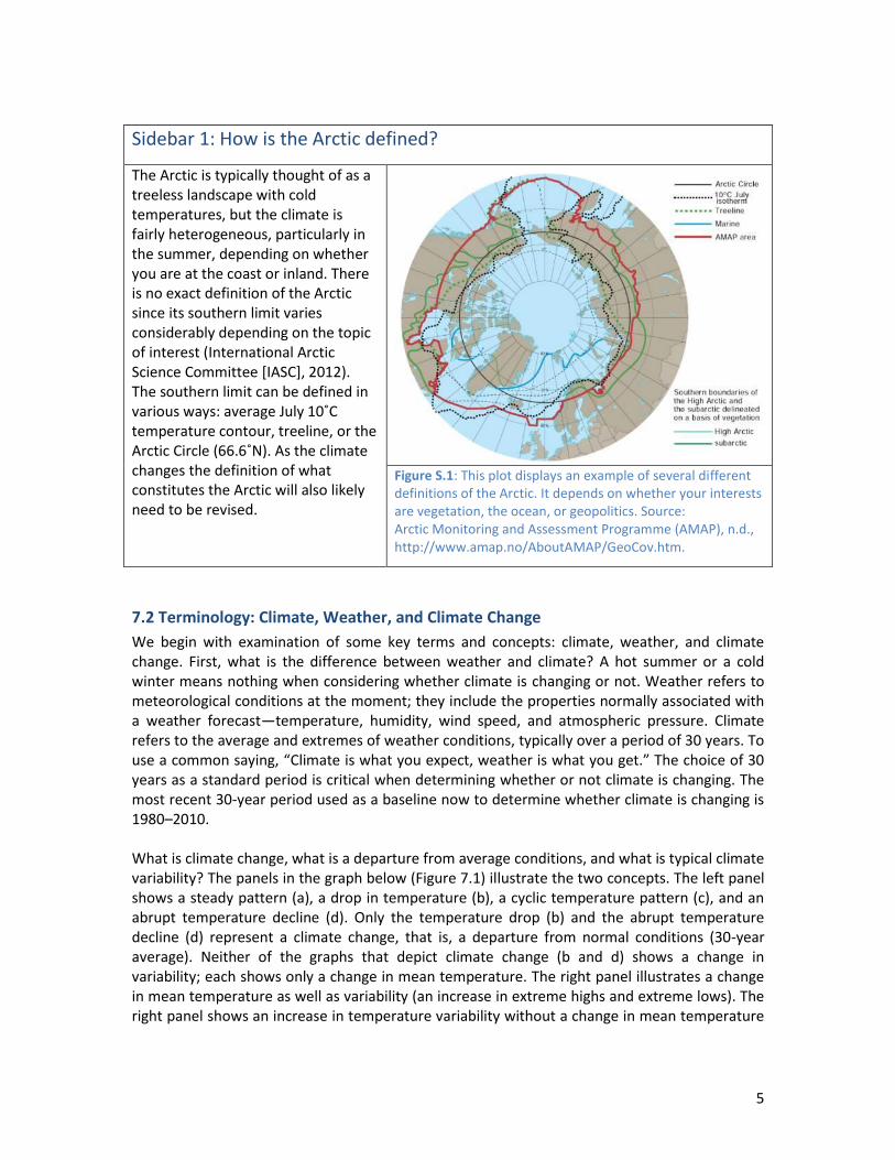
The Arctic is typically thought of as a treeless landscape with cold temperatures, but the climate is fairly heterogeneous, particularly in the summer, depending on whether you are at the coast or inland. There is no exact definition of the Arctic since its southern limit varies considerably depending on the topic of interest (International Arctic Science Committee [IASC], 2012). The southern limit can be defined in various ways: average July 10˚C temperature contour, treeline, or the Arctic Circle (66.6˚N). As the climate changes the definition of what constitutes the Arctic will also likely need to be revised.

Figure S.1: This plot displays an example of several different definitions of the Arctic. It depends on whether your interests are vegetation, the ocean, or geopolitics. Source: Arctic Monitoring and Assessment Programme (AMAP), n.d., http://www.amap.no/AboutAMAP/GeoCov.htm.

7.2 Terminology: Climate, Weather, and Climate Change

We begin with examination of some key terms and concepts: climate, weather, and climate change. First, what is the difference between weather and climate? A hot summer or a cold winter means nothing when considering whether climate is changing or not. Weather refers to meteorological conditions at the moment; they include the properties normally associated with a weather forecast—temperature, humidity, wind speed, and atmospheric pressure. Climate refers to the average and extremes of weather conditions, typically over a period of 30 years. To use a common saying, “Climate is what you expect, weather is what you get.” The choice of 30 years as a standard period is critical when determining whether or not climate is changing. The most recent 30-year period used as a baseline now to determine whether climate is changing is 1980–2010. What is climate change, what is a departure from average conditions, and what is typical climate variability? The panels in the graph below (Figure 7.1) illustrate the two concepts. The left panel shows a steady pattern (a), a drop in temperature (b), a cyclic temperature pattern (c), and an abrupt temperature decline (d). Only the temperature drop (b) and the abrupt temperature decline (d) represent a climate change, that is, a departure from normal conditions (30-year average). Neither of the graphs that depict climate change (b and d) shows a change in variability; each shows only a change in mean temperature. The right panel illustrates a change in mean temperature as well as variability (an increase in extreme highs and extreme lows). The right panel shows an increase in temperature variability without a change in mean temperature

6

(a), a decline in mean annual temperature together with an increase in variability (b), and an abrupt temperature decline along with an increase in variability (c). The 20th century climate record (see Section 3 below) shows a true increase (relative to baseline temperatures) in mean annual temperature. Through the 21st century both mean annual temperature and variability are projected to rise. That means not only that temperatures on average will be higher, but also that there will be more temperatures at the upper and lower ends of the range. Progressively higher temperature records will not be unusual in a warming world.

Figure 7.1: Climate variability versus climate change. Left panels: (a) fluctuations around a steady temperature, (b) a drop in temperature, (c) a cyclic temperature pattern, and (d) an abrupt temperature change. Right panels: (a) change in temperature variability, (b) decline in temperature and an increase in variability, (c) an abrupt temperature change and an increase in variability. Source: Burroughs, 2007. Used with permission of Cambridge University Press/Copyright Clearance Center, Inc. (CCC).

7.3 The Climate Record

The global and Arctic temperature records were examined in depth in the BCS 100 climate module. Since that module was written, several publications have provided assessments of the longer- and shorter-term temperature records for the globe, northern hemisphere, and the Arctic. Below we update the temperature record based on the recent literature published through the end of 2011. Recent Temperature Trends – Globe Global air temperatures in 2012 remained elevated relative to the 20th century mean temperature even though a La Niña cycle (which tends to promote cooling) prevailed during the first three months the year (Figure 7.2). The combined global land and ocean average surface temperature in 2012 was 0.57oC (1.03oF) above the 20th century mean temperature (13.9oC, or 57.0oF), making it the 10th warmest year since records began in 1880; the values for the land and ocean separately were 0.90oC (1.62oF) and 0.45oC (0.81oF) above the 20th century means, making them the 7th and 10th warmest on record, respectively (National Oceanic and Atmospheric

7

Administration [NOAA], 20121). The 12 years in the 21st century (2001–2012) rank among the 14 warmest years (global combined land and ocean temperatures) in the 132-year period of record (NOAA, 2012).

Figure 7.2: Mean surface air temperature anomaly for the period January through December 2012 relative to 1981–2010 mean temperature. Source: NOAA, 2012, http://www.ncdc.noaa.gov/sotc/global/2012/13.

Longer-term Temperature Trends – Northern Hemisphere and the Arctic A recent analysis by Miller et al. (2010) of northern hemisphere air temperature, based on a comprehensive review of climate proxy information (e.g., tree rings and isotope signatures in ice cores and marine sediments), shows variable temperatures over the past 2,000 years but with three distinctly different periods: the Medieval Warm Period between roughly 950 and 1200 AD, the Little Ice Age between roughly 1250 A.D. and 1850 A.D., and a rapid warming during the 20th century (Figure 7.3). Kaufman et al. (2009), based on proxy data from lakes, ice, and tree rings, reported that the amount of 20th century warming in the Arctic is unprecedented over the past 2,000 years. Miller et al. (2010) and Kaufman et al. (2009) showed that temperatures in the northern hemisphere and the Arctic, respectfully, are now the warmest in the past 2,000 years. The Arctic warming that began at the start of the 20th century reversed nearly 2,000 years of cooling (Kaufman et al., 2009).

1 http://www.ncdc.noaa.gov/sotc/global/2012/13

8

Figure 7.3: Multi-decadal and longer-scale variations in global surface air temperature over the past 2,000 years. Source: Miller et al., 2010. Used with permission of Elsevier/CCC.

Arctic Temperature Trends – Late 1800s to Present Arctic surface air temperature anomalies over the past 130 years display a long-term positive trend from the late 1800s to 2010 (Bekryaev et al., 2010) as well as an oscillation with a roughly 50-60 year cycle that has been reported previously (Polyakov et al., 2002). The late 1800s and the 1960s were a generally cool period in the Arctic, while the 1940s and 1990s to the present were characterized by warmer than average temperatures (Figure 7.4, top panel dark line). On top of the large amplitude multidecadal oscillation, there are annual fluctuations in surface air temperature that occur at shorter interannual (1-2 years) to decadal (10 years) time scales (Figure 7.4, top panel). The Arctic temperature increase during 1979–2008 was unusually rapid (1.35oC decade-1), indicating that the recent warming is likely not due to an intrinsic cycle only. The attribution of the long-term trend and the multidecadal variability in the Arctic will be discussed later in this module. The assessment by Bekryaev et al. (2010) notably was based on records from over 441 meteorological stations and represents multiple data sources, including a major previously unutilized data source from Russia. Confidence is highest in the more recent

9

record given that it reflects the most stations and more complete Arctic-wide coverage (Figure 7.4, bottom left panel).

Figure 7.4: Top panel: Composite time series of annual surface air temperature (SAT) anomalies (relative to 1961–2000) for the Arctic, calculated from 441 meteorological stations north of 60oN. Bottom left panel: Locations of meteorological stations used to construct the surface air temperature time series. The inset identifies the number of stations available each year. Bottom right panel: Shaded plot of Arctic autumnal surface air temperature anomalies for each year as a function of distance from the coast. The line plot in the bottom right panel identifies the long-term (1900–2008) trend as a function of distance from the coast. Note that the trends are largest right near the coast and for the warm periods in the Arctic when there is less sea ice in fall along the coast. Source: Bekryaev et al., 2010. Used with permission of American Meteorological Society (AMS)/CCC.

Arctic Amplification The Arctic continues to exhibit a greater increase in temperature (Figure 7.4) than the global average; the phenomenon of more pronounced trends in the Arctic was initially observed by Mitchell (1961) and has been coined “polar amplification” (Broecker, 1975; Schneider, 1975;) or more specifically “Arctic amplification” (Serreze and Barry, 2011). Arctic amplification, which includes accentuation of air temperature increases and decreases as well as variability (relative to global trends), has been attributed to a number of causes. Snow-ice-albedo feedback is one of the primary causes (see Figure 7.3 and related text). As snow cover and ice area decline, the amount of solar radiation that is reflected also decreases, which leads to warming of the Earth’s surface and the overlaying atmosphere. This warming leads to more melting of snow and ice, which warms the surface even more. Another process that has been shown to be important for polar amplification is enhanced heat transport from the tropics (Alexeev et al., 2005). In a warmer climate, tropical convection (the upward movement of surface heat into the upper

10

troposphere) is enhanced, bringing warmer, moister (higher energy) air via northward transport into the Arctic. Computer modeling work by Manabe and Stouffer (1980) showed the largest warming in polar regions is due to increased CO2. The decline of sea ice and the Arctic amplification of surface air temperatures have been investigated in multiple global climate models (Holland and Bitz, 2003). Bekryaev et al., (2010) confirmed in observations that Arctic amplification is related to sea ice changes. They analyzed surface air temperature trends of station data as a function of distance from the coastline (Figure 7.3, bottom right panel) and found that the largest warming (biggest temperature trends) occurs at stations along the coast. In addition, during the cooler period of the 1960s there was no amplification of the anomalously cool temperatures. Further information about Arctic climate, including Arctic amplification, is given in Serreze and Barry (2005).

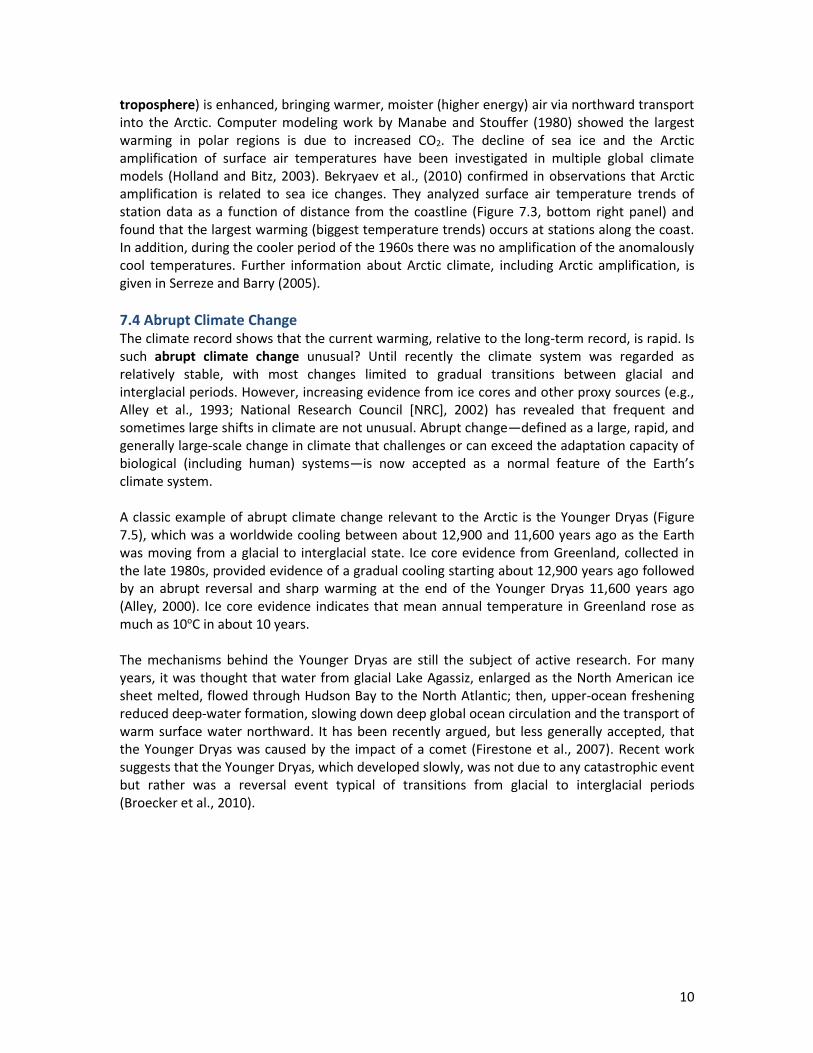
7.4 Abrupt Climate Change The climate record shows that the current warming, relative to the long-term record, is rapid. Is such abrupt climate change unusual? Until recently the climate system was regarded as relatively stable, with most changes limited to gradual transitions between glacial and interglacial periods. However, increasing evidence from ice cores and other proxy sources (e.g., Alley et al., 1993; National Research Council [NRC], 2002) has revealed that frequent and sometimes large shifts in climate are not unusual. Abrupt change—defined as a large, rapid, and generally large-scale change in climate that challenges or can exceed the adaptation capacity of biological (including human) systems—is now accepted as a normal feature of the Earth’s climate system. A classic example of abrupt climate change relevant to the Arctic is the Younger Dryas (Figure 7.5), which was a worldwide cooling between about 12,900 and 11,600 years ago as the Earth was moving from a glacial to interglacial state. Ice core evidence from Greenland, collected in the late 1980s, provided evidence of a gradual cooling starting about 12,900 years ago followed by an abrupt reversal and sharp warming at the end of the Younger Dryas 11,600 years ago (Alley, 2000). Ice core evidence indicates that mean annual temperature in Greenland rose as much as 10oC in about 10 years. The mechanisms behind the Younger Dryas are still the subject of active research. For many years, it was thought that water from glacial Lake Agassiz, enlarged as the North American ice sheet melted, flowed through Hudson Bay to the North Atlantic; then, upper-ocean freshening reduced deep-water formation, slowing down deep global ocean circulation and the transport of warm surface water northward. It has been recently argued, but less generally accepted, that the Younger Dryas was caused by the impact of a comet (Firestone et al., 2007). Recent work suggests that the Younger Dryas, which developed slowly, was not due to any catastrophic event but rather was a reversal event typical of transitions from glacial to interglacial periods (Broecker et al., 2010).

11

Figure 7.5: Record of mean annual temperature (oC) and annual ice accumulation in Greenland over roughly the past 17,000 years before present. Note that current time is at the left end of the x-axis. The Younger Dryas cooling event, which occurred after the last ice age (Pleistocene) came to a close, was between about 12,900 and 11,600 years ago. At the end of the Younger Dryas, roughly 11,600 years ago, mean annual temperature in Greenland increased by about 10oC in about 10 years, and ice accumulation doubled in roughly 3 years. Temperatures (from changes in oxygen isotope) and ice accumulation were determined from ice cores taken from the Greenland ice cap. Source: Adapted from Alley et al., 1993 and available at Past Global Changes (PAGES), 2002, http://www.pages.unibe.ch/products/ppt-slides. Used with permission of Nature Publishing Group/CCC and PAGES.

Understanding the processes responsible for abrupt change is a challenging task, since climate mechanisms are viewed as small changes from an equilibrium state and are generally characterized as linear (i.e., if you double the forcing then you double the response). The study of abrupt change requires nonlinear thinking (i.e., a small forcing change can have a great effect, or a large forcing change can have a small effect) and has classically been studied using simple models such as box or energy balance, where the Earth system is represented by just a few boxes and only some key physical relationships are modeled. These models display multiple equilibria since they contain nonlinear processes, and are a useful tool for studying abrupt change. Box models have been used to study changes in the thermohaline circulation. The thermohaline circulation is a global ocean circulation that is driven by density gradients resulting from changes in temperature and salinity. Energy balance models highlight the role of albedo feedback on climate; when the sea ice edge reaches the midlatitudes it has a runaway albedo feedback effect and this results in a snowball Earth, where the entire globe is covered in snow and ice. There are several abrupt change mechanisms that are of particular concern in a warmer world. Decline of Greenland’s ice sheet, due to accelerated melting, increases fresh water transport into the North Atlantic and promotes formation of a stable surface layer in the ocean (note: fresh water has a lower density than salty water), thereby suppressing deep-water formation. The Meridional Overturning Circulation (MOC) is synonymous with the thermohaline circulation (Figure 7.6) and describes a global circulation loop with sinking motion at high latitudes, southward motion of cool water at depth, and northward motion at the ocean surface. The suppression of deep-water formation by an upper layer of fresh water leads to a slowdown of

12

the MOC reducing poleward heat transport and leading to cooling in the North Atlantic sector. Past evidence suggests that this has happened before (e.g., Younger Dryas). The Greenland ice core record shows that the cooling at the onset of the Younger Dryas was slow, while the warming at its termination was very rapid (Figure 7.5); temperature rose in an abrupt, step-like fashion with an increase of 5–10oC in a few decades or less (Severinghaus et al., 1998). Recent studies that use a combination of observational data and climate model output suggest that the probability of extreme events has increased as a result of the warming climate, such as El Niños or high rainfall events (Min et al., 2011) with floods. Changes in the hydrological cycle characterized by more extreme events have the potential to disrupt agriculture, which depends on steady climate conditions to do well. Ice sheet instabilities, caused when increased underlying melt water accelerates ice transport to the ocean, is a growing concern as recent Greenland ice-sheet melt rates have accelerated (Truffer and Fahnestock, 2007). The interaction between the ocean and ice sheets is an active area of research since the relatively warm ocean waters can rapidly melt floating ice. Ice sheet instability is also an active area of research because the consequences could be catastrophic.

Figure 7.6: Thermohaline circulation (simplified). ACC is the Antarctic Circumpolar Circulation. Source: Kuhlbrodt et al., 2007. Used with permission of John Wiley & Sons/CCC.

The relative stability of climate during recent millennia has contributed to the development of modern human civilization. It has been argued, for example, that the development and continuation of agriculture and agricultural societies, which began roughly 10,000 years ago, required 2,000 years of climate stability (Feynman and Ruzmaikin, 2007). Climate stabilized roughly 10,000 years ago and has remained sufficiently stable so that agriculture became a permanent and catalyzing part of human culture. Agriculture and other basic elements of modern human society will be tested as abrupt, global-scale climate warming continues through this century and beyond.

7.5 Forcing Factors (Positive and Negative)

Forcing factors are the phenomena that influence the Earth’s energy budget and climate; they can be associated with natural variability as well as anthropogenic climate change. One active

13

and challenging area of research is to try to identify the climate variability that can be attributed to "natural” or to “human-induced” forcing factors. It is not always clear how to categorize the forcing factors and even more difficult to link a specific forcing to a climate response. This latter attribution is generally done using models where scientists can limit the forcing factors and evaluate their impacts separately. Attribution of variability to anthropogenic or nonhuman causes is examined later in the module. In this section, the goal is to discuss key forcing factors, highlighting those that are particularly important in the Arctic.

Ocean surface temperature and ocean currents form a lower boundary to the atmosphere and play an important role in forcing the climate on seasonal to longer time scales. The best-known example of an oceanic forcing factor is the El Niño Southern Oscillation (ENSO), which will be discussed further in the next section. ENSO is one of the primary forcing factors for climate in Alaska, with warmer than average winters occurring during a warm ENSO event (Papineau, 2001), and the broader impacts include earlier river ice breakup in Interior Alaska (Bieniek et al., 2011). Warmer air temperatures during ENSO have been linked to enhanced plant productivity on the North Slope of Alaska along the Arctic Ocean (Jia et al., 2003).

The Arctic and North Atlantic surface air temperatures and ocean temperatures display large-amplitude multidecadal variations, the exact cause of which is not well understood as it likely can be forced by a variety of factors. These multidecadal variations are important to consider when calculating ocean and air temperature trends in the Arctic since the strength of the trend is impacted by the phase of these oscillations (Alexeev et al., 2011; Bekryaev et al., 2010). The Arctic and the North Atlantic are connected through the atmosphere as well as the ocean. The atmosphere transports energy from lower latitudes poleward in the form of sensible and latent heat through circulation patterns. The ocean also transports heat poleward with the vast majority entering the Arctic through the North Atlantic. Warm salty water enters the Arctic from the North Atlantic Ocean surface and plunges below the cooler but less salty and lower density Arctic Ocean to form the Atlantic Water layer. This water transports large amounts of heat into the Arctic, the fate of which is an active area of research since it could warm the upper ocean layer and lead to ice melt from below (Polyakov et al., 2005). The ocean, with its large heat capacity, changes slowly in comparison to the atmosphere and thereby moderates the climate. Analogous to the ocean, the cryosphere (snow, permanently frozen ground, sea ice, and glaciers) is a slowly varying component of the climate system. Sea ice cover is itself forced by atmospheric and oceanic circulation and temperature, but modeling studies suggest that there is an impact back on the atmosphere from changes in sea ice. Sea ice changes have been shown to alter large-scale circulation patterns in the Arctic as well as influencing storms (i.e., cyclones responsible for precipitation) in the midlatitudes.

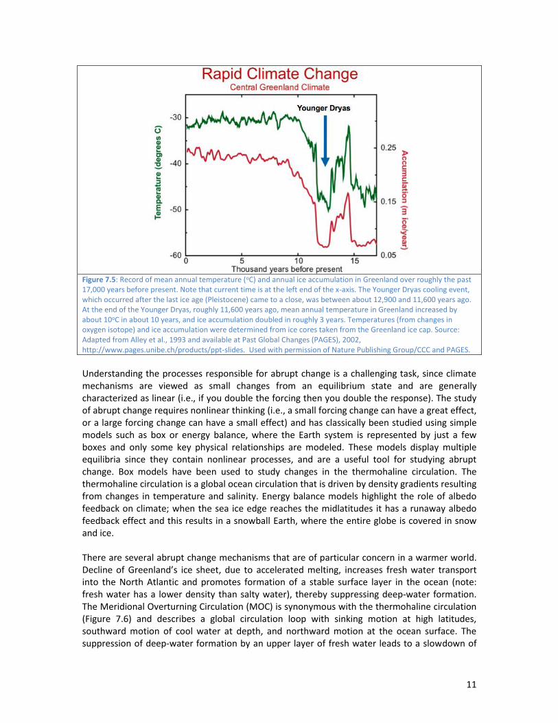
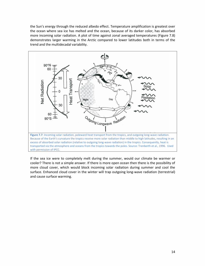
Because the Earth, due to its spherical shape, receives more incoming solar radiation in the tropics and subtropics than at higher latitudes, excess heat (the difference between incoming solar radiation and heat lost due as long-wave radiation to space) flows towards the poles (Figure 7.7). The amount of heat flowing towards the poles increases as the pole-to-equator temperature gradient increases and this poleward heat transport relaxes this temperature gradient (and subsequent heat transport). As a rule, warming is greater over land than the oceans because the oceans have higher heat capacity than land (i.e., ocean temperature changes less than land temperature when heat input is the same). At high latitudes temperature amplification is greatest over land where the snow has melted and land has captured more of

14

the Sun’s energy through the reduced albedo effect. Temperature amplification is greatest over the ocean where sea ice has melted and the ocean, because of its darker color, has absorbed more incoming solar radiation. A plot of time against zonal averaged temperatures (Figure 7.8) demonstrates larger warming in the Arctic compared to lower latitudes both in terms of the trend and the multidecadal variability.

Figure 7.7: Incoming solar radiation, poleward heat transport from the tropics, and outgoing long-wave radiation. Because of the Earth’s curvature the tropics receive more solar radiation than middle to high latitudes, resulting in an excess of absorbed solar radiation (relative to outgoing long-wave radiation) in the tropics. Consequently, heat is transported via the atmosphere and oceans from the tropics towards the poles. Source: Trenberth et al., 1996. Used with permission of IPCC.

If the sea ice were to completely melt during the summer, would our climate be warmer or cooler? There is not a simple answer. If there is more open ocean then there is the possibility of more cloud cover, which would block incoming solar radiation during summer and cool the surface. Enhanced cloud cover in the winter will trap outgoing long-wave radiation (terrestrial) and cause surface warming.

15

Figure 7.8: Surface temperature anomalies (relative to 1961–2000) averaged around different latitude bands. There are larger changes of temperature in the Arctic than in the subtropics. Source: Bekryaev et al., 2010. Used with permission of AMS/CCC.

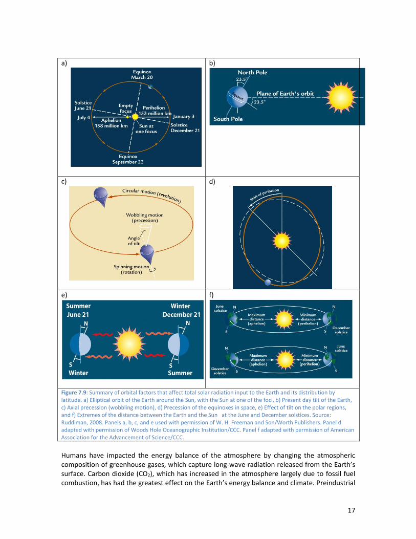
Volcanic eruptions can have a notable but brief impact on the global climate. Explosive tropical volcanic eruptions can inject large amounts of fine ash particles and gases (sulphur dioxide) into the stratosphere, which can block incoming solar radiation to cool the Earth’s surface. The climactically important 1991 eruption of Mount Pinatubo in the Philippines caused global surface cooling of 0.5˚C during the next year (Ruddiman, 2008). The reduction in solar radiation was 3–4 W/m2 (Burroughs, 2007). The fine volcanic dust falls out of the atmosphere relatively quickly, so the cooling effects typically last 1–3 years. Variations in the amount of solar radiation that reaches the Earth affect global surface temperature. The complex dynamics of disturbances on the Sun can change its output of energy, and the most common disturbances are sunspots (temporary dark spots visible on the Sun, which are cooler than surrounding areas). The number of sunspots and the area they cover has an average periodicity of approximately 11 years. It was not until satellite measurements began in the late 1970s that variations in solar irradiance (0.1%) associated with sunspots were quantified. Decreased sunspot activity is linked with lower solar radiation, promoting cooling, whereas increased sunspot activity is linked with higher solar radiation, promoting warming. Feedbacks in the climate system can potentially magnify the impact of the changes in solar irradiance, which is an active area of research. On longer time scales (thousands of years), astronomical variations in the Earth’s orbit around the Sun change the amount of solar radiation arriving at the top of the atmosphere. These variations arise from the Earth-Sun distance through the seasons in the Earth’s elliptical orbit around the Sun and from the tilt of the Earth’s axis of rotation (present day tilt is 23.5˚) (Figure 7.9a-b). This elliptical orbit has the Sun at one of the foci, and since it is not circular the Earth-to-Sun distance varies with season. Presently, the Earth is closest to the Sun on January 3 and farthest from the sun on July 4. The impact of the elliptical orbit changes the amount of solar radiation reaching the top of the atmosphere by a few percent. Recall that the tilt of the Earth’s

16

rotational axis is what is responsible for the seasons. This tilt varies over time from 22.2 to 24.5 degrees and has a periodicity of 41,000 years. If the tilt is large then the amplitude of the seasonal variations is large (i.e., warmer summers and cooler winters); and this has implications for land ice buildup and monsoon circulations, as well as other modes of climate variability. The Earth’s axis also wobbles like a top as it travels around the Sun, known as the axial precession (Figure 7.9c). The elliptical shape of the Earth’s orbit rotates, moving the long and short axis of the ellipse. Together the wobble and turning of the ellipse are called precession of the equinoxes and operate at a frequency of 23,000 years (Figure 7.9d). There are other complex motions due to the gravitational pull of the planets, which can be studied further in Ruddiman (2008). For our purposes we want to know the magnitude of the changes of solar radiation at the top of the atmosphere (Figure 7.7). The tilt is more evident at higher latitudes, and tilt has a major effect on the amount of solar radiation received by the poles in their respective summers and winters (Figure 7.9e). Because of precession the distance of the Earth from the Sun at the solstices and equinoxes is not fixed but instead changes very gradually (Figure 7.9f). Consequently, the Earth can be farther from the Sun during the northern hemisphere summer and closer to the Sun during the northern hemisphere winter, which describes our present state. Together the Earth’s orbital variations play an important role in climate, and their values over the next few thousand years will have an impact on how the climate (e.g., glaciation and monsoons) will evolve.

17

a)

b)

c)

d)

e)

f)

Figure 7.9: Summary of orbital factors that affect total solar radiation input to the Earth and its distribution by latitude. a) Elliptical orbit of the Earth around the Sun, with the Sun at one of the foci, b) Present day tilt of the Earth, c) Axial precession (wobbling motion), d) Precession of the equinoxes in space, e) Effect of tilt on the polar regions, and f) Extremes of the distance between the Earth and the Sun at the June and December solstices. Source: Ruddiman, 2008. Panels a, b, c, and e used with permission of W. H. Freeman and Son/Worth Publishers. Panel d adapted with permission of Woods Hole Oceanographic Institution/CCC. Panel f adapted with permission of American Association for the Advancement of Science/CCC.

Humans have impacted the energy balance of the atmosphere by changing the atmospheric composition of greenhouse gases, which capture long-wave radiation released from the Earth’s surface. Carbon dioxide (CO2), which has increased in the atmosphere largely due to fossil fuel combustion, has had the greatest effect on the Earth’s energy balance and climate. Preindustrial

18

concentration of CO2 was 280 ppm, and as of the end of 2012 the concentration was 394 ppm (NOAA, Earth System Research Laboratory, n.d.2). Methane, another potent greenhouse gas that comes from the anaerobic (lacking oxygen) decomposition of organic matter, has increased, mainly due to increased numbers of domestic cattle and to the expansion of the land area in rice production. Figure 7.10 shows radiative forcing of other greenhouse gases, nitrous oxide, halocarbons, and tropospheric ozone, which have added to warming the atmosphere. Figure 7.11a shows schematically the components of the global energy balance, and Figure 7.11b displays how the surface energy balance is impacted through the enhanced greenhouse effect.

Figure 7.10: Global mean estimates (and ranges) of radiative forcing in 2005, relative to 1750, for greenhouse gases and other agents that influence the Earth’s net energy balance. Included are the spatial scale of effects (local to global) and the assessed level of scientific understanding (LOSU). Volcanic aerosols, which have a cooling effect, are not included because they are episodic. Red bars indicate positive forcing (warming effect); blue bars indicate negative forcing (cooling effect). Source: Intergovernmental Panel on Climate Change [IPCC], 2007a. Used with permission of IPCC.

In the recent decade there has been a growing concern about the role of black carbon soot on bright snow and ice surfaces. While the overall trend for the Arctic is not well known, a recent study by Hirdman et al. (2010) found decreasing trends from 1989–2008 at the stations of Alert (Canada), Barrow (Alaska), and Zeppelin (Svalbard, Norway). Any resident of high latitudes knows from experience that as the Sun returns in the spring and the snow begins to melt, dark dirt particles accumulate on the snow surface and hasten snowmelt. Hansen and Nazerenko (2004) argued that soot on snow yielded a climate forcing of +0.3 W/m2 in the northern hemisphere and may have contributed to recent snow and ice loss. A recent study by Brandt et al. (2011) created artificial snow with controlled soot amounts to investigate the impact of soot

2 http://www.esrl.noaa.gov/gmd/ccgg/trends/#mlo

19

on albedo, and they found that snow particle size was more important for snow albedo changes than black carbon. This works suggests that black carbon is not responsible for large changes in the Arctic. This is an active area of research as scientists strive to understand the magnitude of this forcing with greater accuracy.

Figure 7.11: Top panel: Earth’s radiation balance expressed in watts per square meter. The values next to the arrows for incoming, outgoing, and reflected radiation are mean values for the period March 2000 to May 2004. Bottom panels: Schematic of global radiative balance of the Earth and the role of increased greenhouse gases on the surface energy balance. Sources: Trenberth et al., 2009 (top panel) and National Park Service, 2012, http://www.nps.gov/grba/naturescience/what-is-climate-change.htm (bottom panels). Top panel used with permission of American Meteorological Society (AMS)/CCC.

Land cover and land use change has gained prominence in the climate change discussion as more studies demonstrate that regional climate is strongly influenced by local land use and land cover changes (Dirmeyer et al., 2010). The climate impact due to land cover change includes both warming and cooling and may help to explain some of the observed regional trends in

20

temperature and precipitation. The upcoming Fifth Assessment of the Intergovernmental Panel on Climate Change (IPCC; the IPCC is an international scientific body that synthesizes the current understanding of the world’s climate for use in decision making) will include simulations forced with changes in land surface from agriculture and other human activities in order to account for this effect in simulations of climate change. In the Arctic, land cover changes due to resource development will likely be more important than those due to agriculture. Studies already exist on the impact of oil and gas development on the environment (NRC, 2003), but additional research will be required as the Arctic becomes more accessible due to sea ice decline and resource development increases (e.g., Smith, 2010).

7.6 Large-Scale Atmosphere-Ice-Ocean Circulation Patterns

Figure 7.12: Summary figure of key patterns of climate variability. Source: Solomon et al., 2007. Reprinted with permission of IPCC.

21

To understand climate variability, scientists have focused on investigating key preferred patterns of variability (Figure 7.12), which typically are spatially large patterns that have large amplitudes, and can affect weather in more than one region; linkages between these patterns and weather changes in separate regions of the globe are referred to as teleconnections. The indices are defined based on pressure and temperature anomalies in both the atmosphere and ocean and can switch between phases from the monthly to decadal scales. The opposing phases of these indices describe dramatically different large-scale circulation settings and can have profound effects on weather. Sir Gilbert Walker (Walker, 1924) was the first to identify three recurring patterns of large-scale climate variability based on sparse sea-level pressure station data. He identified the Southern Oscillation Index (SOI) as a sea-level pressure seesaw between the eastern and western equatorial Pacific (Walker and Bliss, 1932). In this 1924 paper, Walker also identified the North Atlantic and North Pacific Oscillations. Several decades later, Bjerknes (1969) discovered how the Southern Oscillation operated and that it was closely tied with sea surface temperatures in the Equatorial Pacific. These indices become more useful once we understand the physical mechanisms behind their variability. Mechanisms of such clarity do not presently exist for the North Pacific and North Atlantic Oscillations (NAO), but are the focus of active research. El Niño (Figure 7.13) and its associated weather is the best understood teleconnection pattern, and means “Little Boy,” referring to the Christ child because Peruvian fishermen commonly observed the phenomenon around Christmas. It represents a broad-scale warming of the eastern Pacific Ocean (to the west of South America). El Niño or ENSO (combining the oceanic El Niño and atmospheric Southern Oscillation phenomena) is caused when prevailing easterly (from the east) trade winds (at Earth’s surface), which normally blow across the Pacific, weaken; and upwelling of nutrient-rich, cold, deep waters along the coast of South America declines sharply. The opposite phase is La Niña, a widespread cooling of the eastern Pacific. ENSO cycles have strong effects on weather over western North America and Australia. For example, El Niño is associated with winter storms in the eastern Pacific, warm winters in Canada, and winter droughts in Australia. ENSO is a powerful example of how ocean-atmosphere interactions affect weather and climate. An ENSO pattern (El Niño or La Niña) typically lasts 6–18 months. The mechanisms behind ENSO are well understood and scientists have had impressive success with ENSO predictions more than 6 months in advance based on this understanding.

22

Figure 7.13: Ocean-atmosphere winter circulation during (from left to right) normal conditions, El Niño, and La Niña, shown with a cross-section through the upper ocean and lower atmosphere. During average climate conditions (left panel) the eastern equatorial Pacific is cool (blue colored water) and the western Pacific is warm (orange colored

water). During El Niño (right panel) the surface is warmer than normal and the convection moves eastward. During La Niña (middle panel) the ocean surface looks more like normal conditions, but the cold water is extended farther westward. The position of the equatorial thermocline (shown as white line), which separates warm surface waters from cooler deeper waters, changes with trade wind strength and influences ocean surface temperatures. Cooler waters prevail at the surface when the thermocline is at a shallower depth. Source: NOAA, 2005, www.cpc.noaa.gov/products/analysis_monitoring/impacts/warm_impacts.shtml.

The Pacific North America (PNA) pattern (Horel and Wallace, 1981) is one of the most important extratropical (outside the tropics) northern hemisphere patterns of climate variability during winter. The positive phase of the PNA is characterized by warmer than normal temperatures in Alaska and western North America, and cooler than normal temperatures in the southeastern United States. The East Asian Jet (a jet is a current of fast moving air found in the upper levels of the atmosphere near the tropopause and guides the path of storms, impacting weather) is closely related to the PNA pattern and is enhanced and shifted eastward during the positive PNA phase. PNA is a natural pattern of variability but is strongly impacted by ENSO and the positive (and negative) PNA phase is associated with ENSO warm (and cold) events. The Pacific Decadal Oscillation (PDO) is a long-term fluctuation of Pacific Ocean temperatures (Figure 7.14). Warm events define conditions when the tropical Pacific and northeast Pacific (especially along the Alaska coast) are above normal and a low-pressure system persists over the Aleutian Islands; conditions are reversed during cool events (Mantua et al., 1997). Each multidecadal phase (positive or negative) can persist for 20–30 years and has strong effects on weather. During warm events air temperatures in northwestern North America are elevated, and precipitation is depressed; the reverse is true during cool events. Warm PDO events can reinforce global warming and can promote broader-scale warming in the northern hemisphere when in phase with a positive NAO phase (Burroughs, 2007).

23

-4

-3

-2

-1

0

1

2

3

4

1900 1920 1940 1960 1980 2000

PDO 12-month smoothed

Figure 7.14: The positive and negative phases of the Pacific Decadal Oscillation (PDO). Top panel: Anomalous wind direction (arrows) and sea surface temperature anomalies in colored shading in degrees Celsius associated with phase changes in the PDO. Bottom panel: Changes in the PDO index since 1900. During the positive (warm) PDO phase, sea surface temperatures in the north central Pacific are cool, and temperatures along the west coast of North America are warm. The opposite is true during the negative (cool) PDO phase (negative PDO index). Source for top panel and PDO index data: Mantua, 2000, http://jisao.washington.edu/pdo/. Used with permission of Nathan Mantua.

Climate anomalies associated with the PDO are prevalent in Alaska and more weakly related to Siberia; most notably station air temperatures went from generally below average to above average in the course of a few years around the change of PDO phase from negative to positive around 1976 (Figures 7.14 and 7.15). The importance of ocean circulation patterns must be kept in mind when trying to interpret annual or even multidecadal temperature changes. Within the context of global-scale warming that has been underway for at least a century, changes in ocean circulation patterns can cause weather changes that seem inconsistent with global warming; conversely, warming at any given location may be due more to a change in an ocean circulation phase than to broader scale warming. This does not discount in any way the influence of other factors (primarily greenhouse gases) that have promoted acute Arctic-wide and global warming. However, changes in ocean circulation patterns need to be considered as dominant key factors that can reinforce or counter global warming, and that can promote warming or cooling and drought or increased precipitation at the regional level for years to decades.

24

Figure 7.15: Mean annual air temperatures for Alaska (1949–2004) with a smoothed line overlaid in black. Source: Alaska Climate Research Center, Geophysical Institute, University of Alaska Fairbanks, 2012, http://climate.gi.alaska.edu/ClimTrends/Change/TempChange.html. Used with permission of Gerd Wendler, University of Alaska Fairbanks.

The Atlantic Multidecadal Oscillation (AMO; see Kerr, 2000, and references therein) characterizes the 20–50 year time scale variability of the North Atlantic Ocean. The AMO is highly correlated with the Atlantic Water (AW) entering the Arctic from the North Atlantic and forming a core of warm salty water under the upper, low-salinity, cool Arctic water. The multidecadal signal is visible in sea ice thickness measurements in the Kara Sea (east of the Barents Sea; blue line in Figure 7.16), AW temperature (red line in Figure 7.16), and surface air temperatures of maritime stations in the Arctic (green line in Figure 7.16). Methods to separate the natural variability from a trend that is typically associated with anthropogenic climate change are not straightforward and are an area of active research.

25

Figure 7.16: Comparative evolution of key components of the Arctic climate system. Composite time series of the Arctic surface air temperature (SAT) anomalies (green), annual intermediate Atlantic Water core

temperature (AWCT) anomalies (red line with dashed segments representing gaps in the record), and anomalies of fast ice thickness in the Kara Sea (Hice, blue): all curves are smoothed using 6-year running mean. Note: The Kara Sea is east of the Barents Sea in the Arctic Ocean. Source: Polyakov et al., 2005. Used with permission of AMS/CCC.

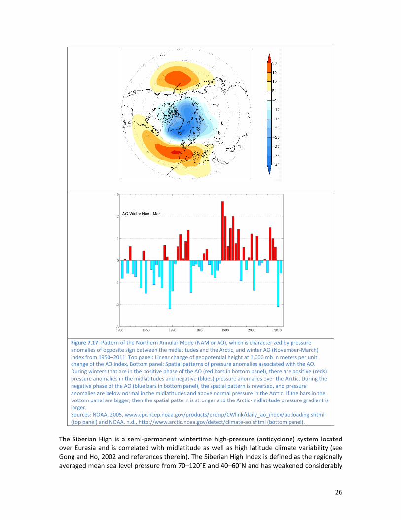
The North Atlantic Oscillation (NAO) is an important pattern of climate variability for eastern North America and west to central Europe (Rogers and van Loon, 1979; van Loon and Rogers, 1978; Walker and Bliss, 1932; van Loon and Rogers, 1978; Rogers and van Loon, 1979). It is defined as the normalized sea level pressure (SLP) anomaly difference between subtropical and midlatitude Atlantic and is a measure of the strength of the pressure gradient between 30oN and 55oN. The pressure gradient is stronger in the positive phase of the NAO, when the North Atlantic storm track is more intense and penetrates further into the Arctic, resulting in generally warmer and wetter conditions in eastern North America and northern Europe (Figure 7.12). During the negative phase of the NAO the north-south pressure gradient is weaker and the storms track across the Atlantic leading to wetter conditions in the Mediterranean and drier ones in northern Europe (Figure 7.12). The NAO is characterized by variability on interannual to multidecadal time scales, but the mechanisms affecting NAO variability are not well understood. The Arctic Oscillation (AO), also called the Northern Annual Mode (NAM) (Thompson and Wallace, 1998), is the pressure difference between the polar regions and the midlatitudes. The AO is often considered to be the atmospheric manifestation the NAO, but more hemispheric in nature. In the positive phase the pressure is below normal in the Arctic and above normal in the midlatitudes (~ 45oN) (Figure 7.17). The AO is particularly useful in describing the polar vortex and has helped to advance knowledge of how the stratosphere interacts with the polar surface (Tanaka and Tokinga 2002).

26

Figure 7.17: Pattern of the Northern Annular Mode (NAM or AO), which is characterized by pressure anomalies of opposite sign between the midlatitudes and the Arctic, and winter AO (November-March) index from 1950–2011. Top panel: Linear change of geopotential height at 1,000 mb in meters per unit change of the AO index. Bottom panel: Spatial patterns of pressure anomalies associated with the AO. During winters that are in the positive phase of the AO (red bars in bottom panel), there are positive (reds) pressure anomalies in the midlatitudes and negative (blues) pressure anomalies over the Arctic. During the negative phase of the AO (blue bars in bottom panel), the spatial pattern is reversed, and pressure anomalies are below normal in the midlatitudes and above normal pressure in the Arctic. If the bars in the bottom panel are bigger, then the spatial pattern is stronger and the Arctic-midlatitude pressure gradient is larger. Sources: NOAA, 2005, www.cpc.ncep.noaa.gov/products/precip/CWlink/daily_ao_index/ao.loading.shtml (top panel) and NOAA, n.d., http://www.arctic.noaa.gov/detect/climate-ao.shtml (bottom panel).

The Siberian High is a semi-permanent wintertime high-pressure (anticyclone) system located over Eurasia and is correlated with midlatitude as well as high latitude climate variability (see Gong and Ho, 2002 and references therein). The Siberian High Index is defined as the regionally averaged mean sea level pressure from 70–120˚E and 40–60˚N and has weakened considerably

27

from the 1980s to 2000 (Gong and Ho, 2002). In the most recent decade the index has risen somewhat but has not returned to pre-1980 values (see Figure 7.18). The Siberian High is negatively correlated with Eurasian temperatures and precipitation during winter (Gong and Ho, 2002), meaning that Eurasia is cooler and drier than normal when the index is more positive. In addition, various studies suggest that it is weakly linked to northern hemispheric climate indices (Panagiotopoulos et al., 2005). This is a pattern of variability that deserves further attention.

Figure 7.18: Time series of the Siberian High Index (December through March mean sea level pressure averaged over 70-120˚E and 40-60˚N) from 1920–2009. This particular index is based on the Trenberth and Paolino (1980) sea-level pressure data set.

Climate indices are meant to simplify relationships, but caution must be exercised when correlating these indices with climate variations without an understanding of the causal physical mechanisms. Trends in climate indices can provide insights into processes operating on a large scale that are related to climate change. Research now underway to separate natural climate variations from anthropogenic climate changes is not straightforward because natural oscillations can be affected by climate change. Global air temperatures showed no upward trend over the past decade, and some skeptics have argued that this indicates that the climate is not changing and that humans have not been the cause of global warming. The more likely explanation is that complex interactions among natural oscillations, ocean storage of heat, and human-induced forcings can result in decadal-length periods when mean global air temperatures are stable. Investigating these climate indices in global climate models simulating the past and comparing how they change in the future is an active area of research to help better project future climate change.

7.7 Linkages Between Climate Change and Human Activity

Earlier in this module we examined the challenge of distinguishing climate change (a long-term shift in climate) from natural climate variability. The strong consensus of climate scientists is that the climate warming since roughly the 1960s represents a true shift in climate that cannot be explained as only an element of natural climate variability. The conclusions of climate scientists that humans have impacted the climate are based on more than 150 years of fundamental research (see The Warming Papers [Supplemental Readings] for key climate science papers). The rise in global mean surface temperature since the middle of the 20th century has been particularly pronounced, and temperatures remain considerably above the baseline mean global temperature. Furthermore, two-thirds of the total warming (0.8oC) from

28

1880 to present has taken place since 1975 (NASA, Earth Observatory, n.d.3). The evidence of warming shown by the instrumental temperature record since the mid-1800s is undebatable. For many people the key issue, and the subject of so much controversy and misunderstanding, is whether the warming is attributable to human activity, or whether it instead represents natural variability. This section of the module focuses on that key issue—attribution, or the degree to which the Earth’s recent warming is attributable to anthropogenic versus natural causes. Answering this question requires a quick review of the Earth’s radiation balance (see Figure 7.10b). Put most simply, the global surface air temperature will rise if radiation inputs are greater than losses. The observed increase in surface air and ocean temperatures reflects that imbalance. It is important to keep in mind that the vast majority of the net energy gain by the globe has been stored in the world’s oceans; the atmosphere, because of its low thermal capacity, represents a very small fraction of the Earth’s total energy increase (Figure 7.19).

Figure 7.19: Energy content changes in different components of the Earth system for two periods: 1961–2003 (light purple) and 1993–2003 (dark magenta). Source: Bindoff et al., 2007. Used with permission of IPCC.

To attribute the Earth’s warming to particular causes scientists carry out what are called “fingerprint studies” in which data for climate variables (e.g., global mean surface temperature, radiation losses to space, temperature profile through the atmosphere) are compared with what would be expected due to natural and anthropogenic forcing factors, including solar radiation, greenhouse gases, and aerosols (see Figure 7.11). The assessments include empirical studies as well as simulations with global climate models. Below appear the results of fingerprinting assessments for single factors as well as for natural, anthropogenic, and natural and anthropogenic factors together. Further information on forcing factors can be found earlier in

3 http://earthobservatory.nasa.gov/Features/WorldOfChange/decadaltemp.php)

29

this module and in the climate module (Module 7) of Introduction to the Circumpolar North (BCS 100). Forcing Factors Perhaps the simplest approach to attribution is to reexamine the graph showing the values for radiative forcing factors (promoting warming or cooling) in 2005 relative to 1750 (see Figure 7.10). Total net radiative forcing (anthropogenic and non-anthropogenic) in 2005 was +1.6 W m-2 compared to 1750. Similar results are obtained if recent values are compared with those in the late 19th century. Hansen et al. (2005), for example, reported that the net change of forcing between 2003 and 1880 was +1.8 W m-2. The anthropogenic signal includes positive (greenhouse gases) and negative forcing factors (aerosols and increasing albedo due to land use change). The non-anthropogenic signal is due to the changes in solar irradiance; the effect of volcanoes, which promote cooling, is not included in the graph because it is short-term (a few years) and because there has been no change in the volcanic activity (frequency and intensity) during the past few centuries. Ninety-four percent of the total net forcing factor difference (1.7 W m-2) between 2005 and 1750 is anthropogenic; 6% is due to solar irradiance. Total greenhouse gas forcing is 2.94 W m-2, and total negative forcing due to aerosols and albedo is 1.24 W m-2. Based on forcing factors alone, 94% of the higher net radiative forcing (promoting warming) in 2005 is due to humans. Greenhouse Gases Multiple lines of evidence indicate that the Earth’s energy imbalance is due primarily to the rise in anthropogenic greenhouse gases. Due to higher concentrations of greenhouse gases (primarily carbon dioxide and methane), the energy and heat content of the troposphere (the lower part of the atmosphere where weather takes place) is increasing; as that heat is radiated, it warms the oceans, the Earth’s surface, and the air above the Earth’s surface. Importantly, the greenhouse gas effect on air temperature is direct and indirect. It is direct through absorption of long-wave radiation (the 2.94 W m-2 forcing) and indirect through the increase in tropospheric water vapor (the dominant greenhouse gas) that results from greenhouse-gas-induced warming (IPCC, 2007a; Lacis et al., 2010). Changes in climate properties are consistent with warming due to anthropogenic greenhouse gases. Let’s examine the evidence. Absorption of Longwave Radiation: Evidence and Consequences Spectrum of the Earth’s long-wave radiation Changes in the spectrum of the Earth’s outgoing long-wave radiation (OLR) over the past several decades provide evidence that the greenhouse gas effect is becoming more pronounced due to rising concentrations of carbon dioxide (CO2), methane (CH4), ozone (O3), and water vapor in the troposphere. The spectra of the Earth’s OLR has been measured periodically (though somewhat sporadically) by satellites since the Nimbus 4 satellite was operational in 1970 and 1971. In a comparison of the spectra from 1997 with spectra measured in 1970 (27 years earlier), Harries et al. (2001) found greater absorption of long-wave radiation in the spectral bands for CO2, CH4, O3, and water vapor in 1997 relative to 1970 (Figure 7.20). In a subsequent study, Griggs and Harries (2004) found that absorption in the greenhouse gas and water vapor bands was greater in 2003 relative to 1997, providing further evidence that the Earth is losing less heat to space because higher greenhouse gas concentrations are increasing heat retention in the troposphere.

30

Figure 7.20: Change in the long-wave radiation released by Earth at the top of the atmosphere to space in 1997 compared to 1970. Absorption by water vapor, which overlaps with methane (CH4), is between 1200 and 1400 cm-1. Source of original graph is Harries et al., 2001; graph shown here is from Cook, 2010. Republished with permission of Nature Publishing Group/CCC and John Cook.

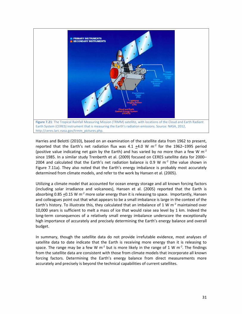
Earth’s net energy flux If the Earth indeed is receiving more energy than it is releasing, can that difference be measured? The answer is a qualified “yes.” Satellites, again starting with the Nimbus satellites, have been measuring incoming solar radiation and outgoing long-wave radiation since the 1970s. Currently those measurements are being made by the Cloud and Earth Radiant Earth System (CERES) instrument aboard three NASA satellites (see Figure 7.21). Satellites cannot directly measure the difference between incoming and outgoing radiation because the difference is very small (less than 1%) relative to the incoming and outgoing flux (341 W m-2) (Trenberth and Fasullo, 2010). However, the incoming and outgoing fluxes each can be tracked over time to determine changes in the Earth’s net radiation balance or net radiation flux (Harries and Belotti, 2010; Trenberth and Fasullo, 2010). This approach is challenging because of sampling and measurement errors and uncertainties associated with the satellites and because the temporal variability (months to decades) of the Earth’s net radiation flux is not well known (Harries and Belotti, 2010).

31

Figure 7.21: The Tropical Rainfall Measuring Mission (TRMM) satellite, with locations of the Cloud and Earth Radiant Earth System (CERES) instrument that is measuring the Earth’s radiation emissions. Source: NASA, 2012, http://ceres.larc.nasa.gov/trmm_pictures.php.

Harries and Belotti (2010), based on an examination of the satellite data from 1962 to present, reported that the Earth’s net radiation flux was 4.1 +4.0 W m-2 for the 1962–1995 period (positive value indicating net gain by the Earth) and has varied by no more than a few W m-2 since 1985. In a similar study Trenberth et al. (2009) focused on CERES satellite data for 2000–2004 and calculated that the Earth’s net radiation balance is 0.9 W m-2 (the value shown in Figure 7.11a). They also noted that the Earth’s energy imbalance is probably most accurately determined from climate models, and refer to the work by Hansen et al. (2005). Utilizing a climate model that accounted for ocean energy storage and all known forcing factors (including solar irradiance and volcanoes), Hansen et al. (2005) reported that the Earth is absorbing 0.85 +0.15 W m-2 more solar energy than it is releasing to space. Importantly, Hansen and colleagues point out that what appears to be a small imbalance is large in the context of the Earth’s history. To illustrate this, they calculated that an imbalance of 1 W m-2 maintained over 10,000 years is sufficient to melt a mass of ice that would raise sea level by 1 km. Indeed the long-term consequences of a relatively small energy imbalance underscore the exceptionally high importance of accurately and precisely determining the Earth’s energy balance and overall budget. In summary, though the satellite data do not provide irrefutable evidence, most analyses of satellite data to date indicate that the Earth is receiving more energy than it is releasing to space. The range may be a few W m-2 but is more likely in the range of 1 W m-2. The findings from the satellite data are consistent with those from climate models that incorporate all known forcing factors. Determining the Earth’s energy balance from direct measurements more accurately and precisely is beyond the technical capabilities of current satellites.

32

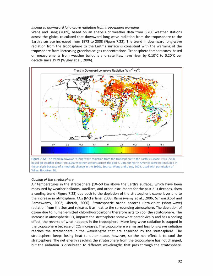
Increased downward long-wave radiation from troposphere warming Wang and Liang (2009), based on an analysis of weather data from 3,200 weather stations across the globe, calculated that downward long-wave radiation from the troposphere to the Earth’s surface increased from 1973 to 2008 (Figure 7.22). The trend in downward long-wave radiation from the troposphere to the Earth’s surface is consistent with the warming of the troposphere from increasing greenhouse gas concentrations. Troposphere temperatures, based on measurements from weather balloons and satellites, have risen by 0.10oC to 0.20oC per decade since 1979 (Wigley et al., 2006).

Figure 7.22: The trend in downward long-wave radiation from the troposphere to the Earth’s surface 1973–2008 based on weather data from 3,200 weather stations across the globe. Data for North America were not included in the analysis because of a methods change in the 1990s. Source: Wang and Liang, 2009. Used with permission of Wiley, Hoboken, NJ.

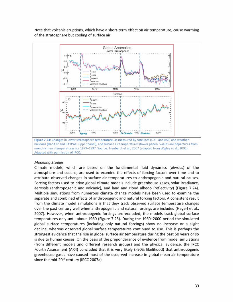
Cooling of the stratosphere Air temperatures in the stratosphere (10–50 km above the Earth’s surface), which have been measured by weather balloons, satellites, and other instruments for the past 2–3 decades, show a cooling trend (Figure 7.23) due both to the depletion of the stratospheric ozone layer and to the increase in atmospheric CO2 (McFarlane, 2008; Ramaswamy et al., 2006; Schwarzkopf and Ramaswamy, 2002; Uherek, 2006). Stratospheric ozone absorbs ultra-violet (short-wave) radiation from the Sun and releases it as heat to the surrounding atmosphere. The depletion of ozone due to human-emitted chlorofluorocarbons therefore acts to cool the stratosphere. The increase in atmospheric CO2 impacts the stratosphere somewhat paradoxically and has a cooling effect, the reverse of what happens in the troposphere. More long-wave radiation is trapped in the troposphere because of CO2 increases. The troposphere warms and less long-wave radiation reaches the stratosphere in the wavelengths that are absorbed by the stratosphere. The stratosphere keeps losing heat to outer space, however, so the net effect is to cool the stratosphere. The net energy reaching the stratosphere from the troposphere has not changed, but the radiation is distributed to different wavelengths that pass through the stratosphere.

33

Note that volcanic eruptions, which have a short-term effect on air temperature, cause warming of the stratosphere but cooling of surface air.

Figure 7.23: Changes in lower stratosphere temperature, as measured by satellites (UAH and RSS) and weather balloons (HadAT2 and RATPAC; upper panel), and surface air temperatures (lower panel). Values are departures from monthly mean temperatures for 1979–1997. Source: Trenberth et al., 2007 (adapted from Wigley et al., 2006). Adapted with permission of IPCC.

Modeling Studies Climate models, which are based on the fundamental fluid dynamics (physics) of the atmosphere and oceans, are used to examine the effects of forcing factors over time and to attribute observed changes in surface air temperatures to anthropogenic and natural causes. Forcing factors used to drive global climate models include greenhouse gases, solar irradiance, aerosols (anthropogenic and volcanic), and land and cloud albedo (reflectivity) (Figure 7.24). Multiple simulations from numerous climate change models have been used to examine the separate and combined effects of anthropogenic and natural forcing factors. A consistent result from the climate model simulations is that they track observed surface temperature changes over the past century well when anthropogenic and natural forcings are included (Hegerl et al., 2007). However, when anthropogenic forcings are excluded, the models track global surface temperatures only until about 1960 (Figure 7.25). During the 1960–2000 period the simulated global surface temperatures (including only natural forcings) show no increase or a slight decline, whereas observed global surface temperatures continued to rise. This is perhaps the strongest evidence that the rise in global surface air temperature during the past 50 years or so is due to human causes. On the basis of the preponderance of evidence from model simulations (from different models and different research groups) and the physical evidence, the IPCC Fourth Assessment (AR4) concluded that it is very likely (>90% likelihood) that anthropogenic greenhouse gases have caused most of the observed increase in global mean air temperature since the mid-20th century (IPCC 2007a).

34

The same findings have been obtained from individual modeling studies. Tett et al. (2002), for example, reported that natural forcings from about 1910–1950 showed an increase due to an increase in solar irradiance and a lack of volcanic eruptions and that natural forcings promote cooling after the 1960s onward. Over the entire 20th century Tett and colleagues found that natural forcings made no net contribution to the observed global air temperature change because the positive forcings (promoting warming) in the first half of the 20th century were canceled out by the negative forcings (promoting cooling) in the second half of the century. Notably, no trends in solar irradiance other than the 11-year oscillation cycle have been detected over the past few decades (Lacis et al., 2010); in fact, if anything, solar irradiance, which has a small impact on changes in global temperature during the 20th century, has shown a downward trend since 1987 (Lockwood, 2008). Braganza et al. (2004), in another modeling simulation study, found that anthropogenic forcings accounted for almost all the observed changes in global mean air temperature during 1946–1995. There is strong evidence that humans are influencing surface air temperatures not only at the global level but also at the continental scale. A computer modeling study showed that the rise in surface air temperatures since about the 1970s for all six populated continents (North America, South America, Africa, Europe, Asia, and Australia) can be explained only when anthropogenic forcings are included (Hegerl et al., 2007) (Figure 7.26). In a more recent review Stott et al. (2010) reported that human-caused temperature changes have now been detected on all continents including Antarctica.

Figure 7.24: Example of forcing factors used to drive model simulations of global climate change. LLGHG = Long-lived greenhouse gases. Land use is the increase in albedo (reflectivity) due to land use change (e.g., conversion of forests to tilled land). Source: Forster et al., 2007. Used with permission of IPCC.

35

Figure 7.25: Observed (black) and simulated (red or blue) global mean surface air temperature anomalies 1901–2000. Simulated and observed temperatures when both anthropogenic and natural forcing factors were included (top panel) and when anthropogenic forcing factors were excluded (bottom panel). The top panel includes 58 simulations from 14 models; the bottom panel includes 19 simulations from five models. The anomalies are the difference in mean annual air temperature relative to the mean temperature for the 1901–1950 period. Source: Hegerl et al., 2007. Used with permission of IPCC.

Figure 7.26: Observed and modeled surface air temperatures for the globe and continents. Blue bands show results for 19 simulations of 5 climate models that include only natural forcings; pink bands show results for 58 simulations from 14 climate models. Black line shows observed values. Source: Hegerl et al., 2007. Used with permission of IPCC.

36

7.8 Climate Change Projections: Temperature and Precipitation

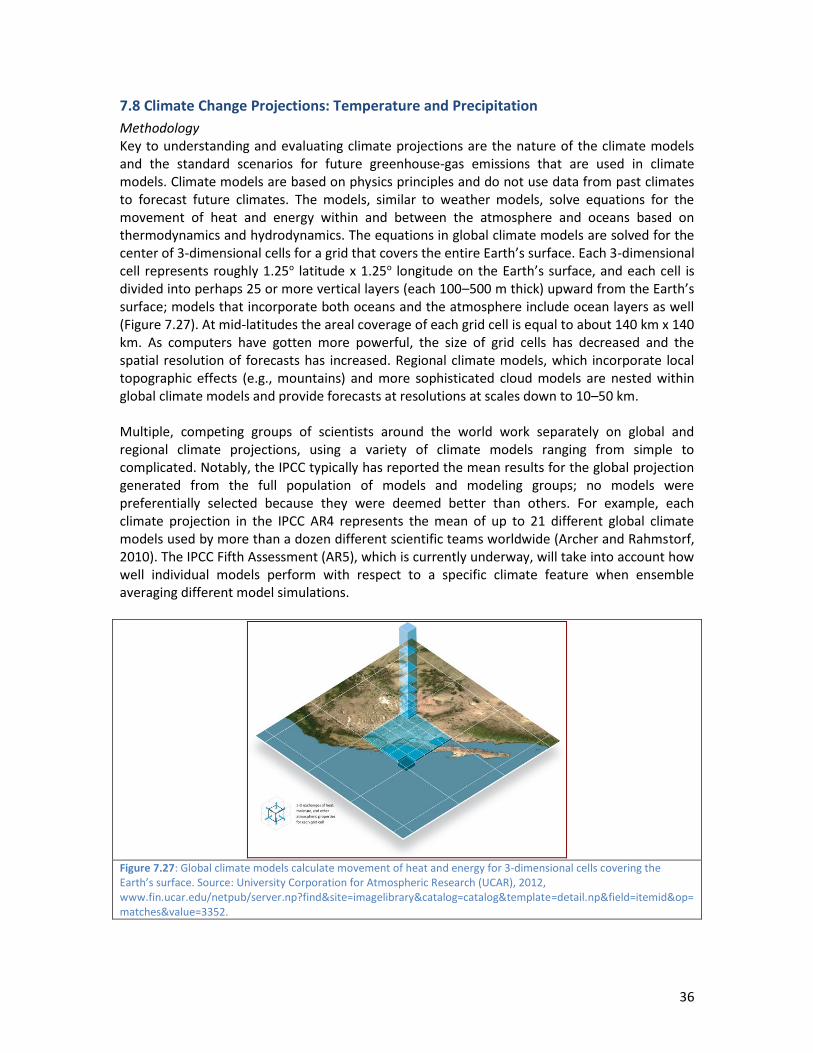
Methodology Key to understanding and evaluating climate projections are the nature of the climate models and the standard scenarios for future greenhouse-gas emissions that are used in climate models. Climate models are based on physics principles and do not use data from past climates to forecast future climates. The models, similar to weather models, solve equations for the movement of heat and energy within and between the atmosphere and oceans based on thermodynamics and hydrodynamics. The equations in global climate models are solved for the center of 3-dimensional cells for a grid that covers the entire Earth’s surface. Each 3-dimensional cell represents roughly 1.25o latitude x 1.25o longitude on the Earth’s surface, and each cell is divided into perhaps 25 or more vertical layers (each 100–500 m thick) upward from the Earth’s surface; models that incorporate both oceans and the atmosphere include ocean layers as well (Figure 7.27). At mid-latitudes the areal coverage of each grid cell is equal to about 140 km x 140 km. As computers have gotten more powerful, the size of grid cells has decreased and the spatial resolution of forecasts has increased. Regional climate models, which incorporate local topographic effects (e.g., mountains) and more sophisticated cloud models are nested within global climate models and provide forecasts at resolutions at scales down to 10–50 km. Multiple, competing groups of scientists around the world work separately on global and regional climate projections, using a variety of climate models ranging from simple to complicated. Notably, the IPCC typically has reported the mean results for the global projection generated from the full population of models and modeling groups; no models were preferentially selected because they were deemed better than others. For example, each climate projection in the IPCC AR4 represents the mean of up to 21 different global climate models used by more than a dozen different scientific teams worldwide (Archer and Rahmstorf, 2010). The IPCC Fifth Assessment (AR5), which is currently underway, will take into account how well individual models perform with respect to a specific climate feature when ensemble averaging different model simulations.

Figure 7.27: Global climate models calculate movement of heat and energy for 3-dimensional cells covering the Earth’s surface. Source: University Corporation for Atmospheric Research (UCAR), 2012, www.fin.ucar.edu/netpub/server.np?find&site=imagelibrary&catalog=catalog&template=detail.np&field=itemid&op=matches&value=3352.

37

The projections produced by climate scientists are based on a number of different scenarios for future greenhouse-gas emissions that have been developed by IPCC and presented in the Special Report on Emissions Scenarios, commonly referred to as SRES (IPCC, 2000). The emissions scenarios, which were developed by over 50 specialists spanning a range of disciplines (including economists, social scientists, and geoscientists) and from 18 countries, are based upon four different storylines for demographic development (size of human population), socioeconomic development, and technological change. They include projections for both greenhouse gases (warming effect) and anthropogenic aerosols (cooling effect) in the atmosphere and take into account gains (emissions) and losses (e.g., return to oceans and vegetation via uptake). The scenarios include human effects on climate only, not natural factors such as volcanoes and solar variability. Most likely, changes in those factors over the next couple centuries will be small (an increase or decrease of a few tenths of a degree C for solar variability) or transitory (a few years of cooling from volcanoes). The scenarios don’t include any surprises, such as a large release of methane hydrates from the sea bottom or major changes in ocean circulation patterns; they do not include possible mitigation measures (removal and storage of atmospheric CO2); and they are not given probabilities of occurrence (IPCC, 2000). Each scenario is as likely or unlikely as another. Climate modeling groups around the world use these standardized scenarios (see Figure 7.28 legend for description) to forecast temperature changes during and beyond the current century. Note that for the IPCC AR5, the scenarios are being constructed differently; they are based on representative concentration pathways for greenhouse gases and variously incorporate mitigation measures. How is the quality of the models and their projections assessed? The quality of models is determined by how well the models (not driven by climate data) reproduce the past climate. Scientists have confidence in the models because they accurately track 20th century climate trends from the global to continental and regional scales (see previous section and Figure 7.28). The quality of climate projections should continue to improve as computer power increases and as models better incorporate the interactions between the atmosphere and other Earth-system components such as sea ice, large-scale ocean circulation cycles (e.g., the AO and ENSO), land surface, and biogeochemistry. Projections In 2007 the IPCC released climate-model projections for global 21st century climate based on the SRES (greenhouse-gas emissions scenarios) described above. The models forecast a mean global temperature rise of about 0.2oC per decade for the next two decades, and then varying rates of continued warming through the 21st century for the different scenarios. Warming over the 21st century is forecast to range from 0.6oC if atmospheric CO2 remains at year 2000 levels to 4.0oC for the A1F1 scenario that assumes rapid economic growth, a population that peaks in mid-century, and continued high reliance on fossil fuels. One key feature of the forecasts is that warming is not spatially uniform across the globe. Warming is forecast to be greater over land than over oceans and greatest at high latitudes (Figure 7.29). Increases in the Arctic are roughly twice the global average and range from roughly 4oC to 7.5oC for the mid-range A1B scenario (economic growth, population that peaks in mid-century, and a blend of fossil fuel and non-fossil fuel energy sources). Notably, actual greenhouse gas emissions for the first decade in the 21st century (2000–2009) have exceeded the projected emissions of the most extreme (A1F1) IPCC scenario.

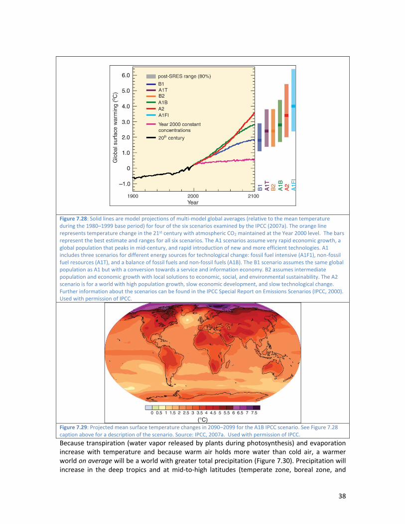
38

Figure 7.28: Solid lines are model projections of multi-model global averages (relative to the mean temperature during the 1980–1999 base period) for four of the six scenarios examined by the IPCC (2007a). The orange line represents temperature change in the 21st century with atmospheric CO2 maintained at the Year 2000 level. The bars represent the best estimate and ranges for all six scenarios. The A1 scenarios assume very rapid economic growth, a global population that peaks in mid-century, and rapid introduction of new and more efficient technologies. A1 includes three scenarios for different energy sources for technological change: fossil fuel intensive (A1F1), non-fossil fuel resources (A1T), and a balance of fossil fuels and non-fossil fuels (A1B). The B1 scenario assumes the same global population as A1 but with a conversion towards a service and information economy. B2 assumes intermediate population and economic growth with local solutions to economic, social, and environmental sustainability. The A2 scenario is for a world with high population growth, slow economic development, and slow technological change. Further information about the scenarios can be found in the IPCC Special Report on Emissions Scenarios (IPCC, 2000). Used with permission of IPCC.

Figure 7.29: Projected mean surface temperature changes in 2090–2099 for the A1B IPCC scenario. See Figure 7.28 caption above for a description of the scenario. Source: IPCC, 2007a. Used with permission of IPCC.

Because transpiration (water vapor released by plants during photosynthesis) and evaporation increase with temperature and because warm air holds more water than cold air, a warmer world on average will be a world with greater total precipitation (Figure 7.30). Precipitation will increase in the deep tropics and at mid-to-high latitudes (temperate zone, boreal zone, and

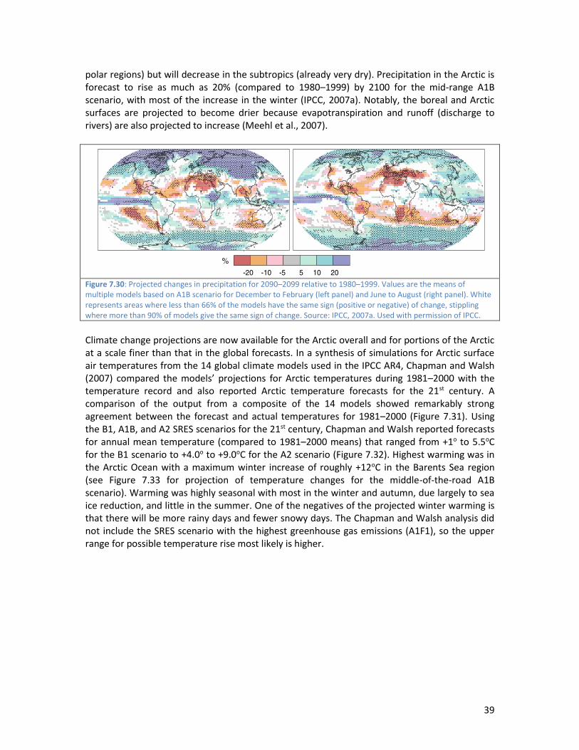
39

polar regions) but will decrease in the subtropics (already very dry). Precipitation in the Arctic is forecast to rise as much as 20% (compared to 1980–1999) by 2100 for the mid-range A1B scenario, with most of the increase in the winter (IPCC, 2007a). Notably, the boreal and Arctic surfaces are projected to become drier because evapotranspiration and runoff (discharge to rivers) are also projected to increase (Meehl et al., 2007).

Figure 7.30: Projected changes in precipitation for 2090–2099 relative to 1980–1999. Values are the means of multiple models based on A1B scenario for December to February (left panel) and June to August (right panel). White represents areas where less than 66% of the models have the same sign (positive or negative) of change, stippling where more than 90% of models give the same sign of change. Source: IPCC, 2007a. Used with permission of IPCC.

Climate change projections are now available for the Arctic overall and for portions of the Arctic at a scale finer than that in the global forecasts. In a synthesis of simulations for Arctic surface air temperatures from the 14 global climate models used in the IPCC AR4, Chapman and Walsh (2007) compared the models’ projections for Arctic temperatures during 1981–2000 with the temperature record and also reported Arctic temperature forecasts for the 21st century. A comparison of the output from a composite of the 14 models showed remarkably strong agreement between the forecast and actual temperatures for 1981–2000 (Figure 7.31). Using the B1, A1B, and A2 SRES scenarios for the 21st century, Chapman and Walsh reported forecasts for annual mean temperature (compared to 1981–2000 means) that ranged from +1o to 5.5oC for the B1 scenario to +4.0o to +9.0oC for the A2 scenario (Figure 7.32). Highest warming was in the Arctic Ocean with a maximum winter increase of roughly +12oC in the Barents Sea region (see Figure 7.33 for projection of temperature changes for the middle-of-the-road A1B scenario). Warming was highly seasonal with most in the winter and autumn, due largely to sea ice reduction, and little in the summer. One of the negatives of the projected winter warming is that there will be more rainy days and fewer snowy days. The Chapman and Walsh analysis did not include the SRES scenario with the highest greenhouse gas emissions (A1F1), so the upper range for possible temperature rise most likely is higher.

40

Figure 7.31: Observed (top row) and projected (bottom row) seasonal mean surface air temperatures for the Arctic during the 1981–2000 period. The observed data (ERA-40) are from the European Centre for Medium-Range Weather Forecasts, and the projected data are from a composite of 14 global climate models used in the IPCC AR4. Source: Chapman and Walsh, 2007. Used with permission of AMS/CCC.

Figure 7.32: Simulated (1900–2000) and projected (2000–2100) mean surface air temperatures in the Arctic for three IPCC emissions scenarios (B1, A2, and A1B) from 14 global climate models. The letters A through N designate each of the global climate models used. Source: Chapman and Walsh, 2007. Used with permission of AMS/CCC.

41

Figure 7.33: Arctic surface-air temperature change, relative to 1981–2000, for 2070–2089 based on the A1B greenhouse gas emissions scenario forecast by a composite of 14 global climate models. Source: Figure 13 from Chapman and Walsh, 2007. Used with permission of AMS/CCC.

Regional climate-model projections, which are of greater interest to government officials, the business community, nongovernmental organizations, and the general public because of their higher resolution (25–50 km), have become available over the past decade for North America, Europe (including most of western Russia), and Greenland. Most regional models for the Arctic and the eight Arctic nations show the same patterns as those forecast by the global models for high latitudes—amplified warming, concentrated in the winter and fall, and higher annual precipitation largely concentrated in the winter—but with finer spatial variability. Forecast changes have greatest spatial variability in areas with complex topography, particularly in mountainous regions; and warming tends to be most elevated farther from the coast, where the ocean moderates air temperature changes (Christensen et al., 2007). In the Arctic that pattern can be altered; late formation of coastal sea ice in the fall and earlier recession of coastal sea ice in the spring can amplify warming along the coast (see Figure 7.3). A challenge for regional-scale forecasts in the Arctic is capturing low frequency (sometimes multidecadal) climate patterns such as the El Niño Southern Oscillation (ENSO) and the Northern Annual Mode. Regional models provide finer-scale forecasts (especially for precipitation) which give great detail but must be used with care as errors in both the global model as well as the regional model impact the results; a projection with higher spatial precision does not necessarily mean that it is more accurate (Kerr, 2011). Reducing the uncertainty of regional-scale projections is essential for their use in establishing, funding, and implementing adaptation and mitigation strategies. We can’t plan for the future at the regional scale unless the uncertainty level for projections is low. Although a description of available regional-scale forecasts for all Arctic countries and Arctic areas is beyond the scope of this module, we present regional-scale temperature and precipitation projections for Europe (including Norway, Denmark, and Sweden) as an example. The most recent regional scale forecasts for Europe are from the ENSEMBLES project, a large climate change project funded by the European Commission and involving a consortium of 66 institutes (from 20 countries) that carry out climate change research (van der Linden and Mitchell, 2009). The core of the project was the use of an ensemble of multiple climate models (via independent research groups) to improve the reliability of climate projections and impacts based on the IPCC greenhouse-gas emissions scenarios (SRES). The projections (Figure 7.34) show 3.5–4.0OC warming and a 12–20% precipitation increase for Scandinavia for the A1B (mid-

42

range) scenario in 2071–2100 compared with 1961–1990. Notably, the temperatures forecast for Scandinavia under the A1B (middle-of-the-road) scenario are much higher than those ever experienced by humans in the Circumpolar North. Forecast temperatures for the A1F1 scenario (greatest greenhouse-gas emissions) would be even higher.

Figure 7.34: Projected changes in annual mean surface air temperature (degrees C; top panel) and annual precipitation (%; bottom panel) for Europe in 2071–2100 relative to 1961–1990 mean. Values are the mean of an ensemble of regional climate models and are based on the A1B SRES (mid-range) scenario. Source: van der Linden and Mitchell, 2007. Used with permission of ENSEMBLES.

7.9 Recent and Future Biophysical Impacts of Climate Change in the North

General Principles Vulnerability, resilience, adaptive capacity, and capacity for potential benefit are key to understanding the impacts of climate change on human-biophysical systems. Vulnerability is

43

susceptibility to be harmed. Resilience is the capacity for a system to return to pre-disturbance or near pre-disturbance conditions, without loss of essential character and function, after a disturbance or application of new impacts or pressures. Adaptive capacity is the capacity of a system to adapt to impacts, pressures, or disturbances without harm and potential benefit. For biological systems this can include natural tolerance, genetic diversity, biological plasticity, the degree of functional redundancy among components, and the ability to move. For human systems adaptive capacity includes the resources of a country (e.g., capital, infrastructure, technology, education system, and work force training) as well as political factors. Every system has a resilience limit. A system with little or no adaptive capacity will suffer a breakdown of structure and essential functions when its resilience limit is exceeded. Climate change, which includes changes of seasonal and average temperatures and precipitation, growing season, and other aspects of climate, has extensive effects (some magnified and many nonlinear) on the coupled human-biophysical systems of the Arctic. Those effects, particularly those on biological and human systems, are not simple or easy to understand. Some aspects of climate change will be positive, others will be more serious than expected, and some will be totally unexpected (Archer and Rahmstorf, 2010). Impacts in general are expected to be large because of the high rate of climate change, the forecast temperatures (a large warming in addition to the warm temperatures typical of an interglacial period), and the increased likelihood of extreme events; in addition, an intensely fragmented landscape (due to human activity) will make migration of plants and animals difficult as climate shifts (Archer and Rahmstorf, 2010). In many cases the migration speed of plant and animal species will be slower than the velocity of climate change across the landscape (Loarie et al., 2010). Identifying and forecasting climate change effects on biological systems is challenging because climate change influences not only individual organisms and individual species, but also populations of organisms that are shaped by both negative interactions (e.g., competition and predation) and positive ones. At the organismal or species level, climate (together with negative or positive interactions between different species) largely determines an organism’s ecological niche and its landscape distribution. A niche is the range of a combination of factors (climate being one) that defines the conditions in which an organism or species can survive, grow, and reproduce successfully. As climate changes, the spatial distribution of plants (in order to remain in the niche) will adjust as long as the rate of climate change does not outpace the migration speed of plants and as long as plants do not encounter major differences in competition or physical barriers (e.g., a mountain range). Plant distributions on the landscape can be out of sync with new climate regimes because plant movements, generally governed by seed dispersal, may be slow or influenced by competition. If plants do not move (or move slowly), climate changes may lead to higher or lower growth rates, increased or decreased health, and in some cases extirpation (loss of species in an area) or extinction (complete loss of a species). Animals generally have capacity to move as climate changes, but they may face absence of corridors or pathways, changes in competition that can be detrimental or positive, and alteration of food and water resources. In the case of alpine plants and animals, increased warming may force organisms to increasingly higher elevations with an end point being extirpation or extinction. For plants and animals that border the Arctic coastline, their north-to-south habitat ranges will be compressed considerably as the climate warms.

44

Biophysical Impacts of Recent Warming: Meta-analysis Thus far, the global mean temperature rise of 0.74oC and other associated climate changes during the past 100 years have been small. Has such a small change had an effect on biophysical systems? The answer is yes, and in some cases the effects have been dramatic. Isolating the effects of the 20th century temperature rise on a single plant or animal species or a single physical factor is difficult, and in many cases responses are idiosyncratic. A more informative approach is to identify common responses from a broad survey of studies and for a large number of species and biological and physical systems. Such meta-analyses have yielded compelling results. In an examination of 29,000 observational data series that spanned at least 20 years, ended in 1990 or later, and showed significant change over time, the IPCC (2007b) found that more than 89% of the changes are consistent with climate warming. In the polar regions (Arctic plus Antarctic), 91% of physical changes and 100% of biological changes are consistent with warming. The IPCC survey and as well as other meta-studies have shown that the relatively minor climate changes of the 20th and early 21st century are already influencing human activities and livelihoods (Carter, 2010), with a mixture of negative, neutral, and positive consequences. Biophysical Impacts of Climate Change: Positive or Negative? Are the observed and forecast changes on balance negative or positive? Often the answer depends on what is affected, the nature and degree of the climate change effect, and adaptive capacity. Key observed and forecast impacts of warming across the globe are summarized in Figures 7.35 and 7.36. A critically important point is that impacts depend on both the amount of climate change as well as changes in the frequency and range of extreme events. Below we address observed and forecast climate change effects on components that are fundamental to the health and fundamental nature of the Arctic—sea level, sea ice, marine mammals, ecosystems, and natural resources. The future of Arctic peoples depends largely on how these different components respond.

45

Figure 7.35: Significant changes in physical systems, biological systems, and surface air temperatures during 1970–2004. The data are from 29,000 data series (each spanning at least 20 years) from roughly 75 studies. The 2x2 boxes show the number of significant changes and the percentage of changes consistent with warming for physical and biological systems by region and globally. The regions are North America (NAM), Latin America (LAM), Europe (EUR), Africa (AFR), Asia (AS), Australia and New Zealand (ANZ), and polar regions (PR). Source: IPCC, 2007b. Used with permission of IPCC.

46

Figure 7.36: Examples of global impacts of climate warming for a range of global mean air temperature increases relative to mean global air temperature during the 1980–1999 period. Dotted lines indicate that impacts will continue with increasing temperature. The beginning position of the text indicates the temperature at which each impact is forecast to begin. Impacts will depend on adaption capacity, amount of climate change, and in some cases socioeconomic factors. Extreme events are an important factor not included in the figure and in some cases may have greater impact in the short term than changes in mean climate regimes. Source: IPCC, 2007b. Used with permission of IPCC.

Sea Level Rise Sea level rise is the climate-warming consequence that may have the greatest effect on people because so many cities and towns, including those in the Arctic, are located on the coast; worldwide 634 million people live less than 10 m above sea level (McGranahan et al., 2007). The causes of sea level rise are (1) the expansion of water as it warms, and (2) increased water flows to the ocean as land-based ice (glaciers and ice sheets) melts. The melting of Arctic sea ice, which is not land-based, does not raise sea levels because the volume of floating ice is equivalent to the volume of water displaced. During the last ice age, which ended roughly 15,000 years ago, global mean sea level was roughly 120 m lower than sea level today and rose as glacial ice melted. The ice currently in Greenland and Antarctica would raise ocean water levels 7 m and 57 m, respectively, if it all melted (Archer and Rahmstorf, 2010); though such complete ice loss in these regions is implausible, a small proportional reduction in ice in these two regions would raise sea levels substantially (Table 7.1).

47

Table 7.1: Area, volume, and sea level equivalent of snow on land, sea ice, ice, seasonally frozen ground, and permafrost. Source: Lemke et al., 2007. Used with permission of IPCC.

Global sea level is rising. Direct measurements of sea level are based upon tide gauges and, starting in the early 1990s, upon satellites that use radar altimeters to precisely measure their height above sea level (Henson, 2011). The measurements show that sea level rose during the 20th century by about 17 cm; since the early 1990s sea level has risen at an increased rate of roughly 3 mm yr-1 (Figure 7.37) (Bindoff et al., 2007; Rahmstorf, 2007). Sea levels prior to the period of direct measurements, which began in the late 1800s, have been calculated from proxy data (indirect data). Based on those data, sea level was stable for nearly the past 2,000 years; the rise in sea level is a recent phenomenon (Archer and Rahmstorf, 2010). The amount of sea level rise during the past century may seem unimpressive. However, the hazard of sea level rise is the not the rise per se but rather how it increases damage due to the high sea levels during storm surges (Bindoff et al., 2007). Projections for sea level rise by the end of the current century are more troubling. Projecting sea level rise is tricky because understanding of the dynamics of the Greenland and Antarctic ice sheets, which each dwarf the ice volume of other land-based ice (mostly glaciers), is poor and because several recent studies (e.g., Rignot and Kanagaratnam, 2006, and Rignot et al., 2008) have shown that ice sheets in Greenland and west Antarctica are melting at accelerating rates. Rignot and Kanagaratnam (2006) reported, for example, that the Greenland ice sheet was melting roughly twice as fast (and adding twice as much water to the sea) in 2006 as it was in 1996. The IPCC, which did not include increases in the dynamics of the Greenland and Antarctic ice sheets in the models used to calculate future sea level (Archer and Rahmstorf, 2010), projected sea level to rise 18–59 cm (relative to the 1980–1999 mean) by 2090–2099 (Figure 7.38) (Bindoff

48

et al., 2007). The amount of sea level rise is not uniform globally because of non-uniform differences in ocean temperatures and salinity related to changes in ocean circulation driven by climate change (IPCC, 2007b). Sea level rise by 2080–2099 is projected to be 5–20 cm higher in the Arctic compared to the global average (Archer and Rahmstorf, 2010; Meehl et al., 2007). The IPCC noted that including accelerated melting rates for the Greenland and Antarctic ice sheets (as observed recently) could add another 10-20 cm to the projected rise (Henson, 2011; Meehl et al., 2007). Notably, the rate of sea level rise during the 1961–2003 period was about 50% higher than IPCC projections for the same period (Archer and Rahmstorf, 2010). Other investigators have taken different approaches to projecting future sea level rise. Rahmstorf (2007) used a relationship between global mean surface air temperature and sea level during the period 1881–2001 and projected a sea level rise of 0.5–1.4 m in 2011 relative to the 1990 level. More recently Jevrejeva et al. (2012) reported projected sea level rise ranging from 0.57–1.10 m by 2100, and perhaps more importantly a continuation of sea level rise for 500 years, ranging from 1.84 m to 5.49 m by the year 2500. Sea level rise in the Arctic would put many coastal cities in the Arctic at risk (e.g., Churchill, Kirkenes, Murmansk, and Anchorage), including their shipping facilities, oil- and gas-industry infrastructure, central business districts, and residential centers. Particularly at risk would be permafrost-underlain coastlines, which would be more susceptible to erosion from wave action and storm surges as permafrost thaws.

Figure 7.37: Top panel: Rate of sea level rise based on direct observations (red line) and calculated from a relationship between air temperature and sea level (blue line). Bottom panel: Sea level relative to 1990 obtained from observations (red line and red squares) and calculated from global mean air temperature (blue line). The red line represents a smoothing of the annual sea level data. Source: Rahmstorf, 2007. Used with permission of American Association for the Advancement of Science/CCC.

49

Figure 7.38: Past and forecast global sea level changes relative to the 1980–1999 mean. The forecast changes are based on the SRES A1B scenario (mid-range greenhouse gas emissions). Global sea level measurements were not available prior to 1870. Source: Bindoff et al., 2007. Used with permission of IPCC.

Ice and Snow In the Arctic, sea ice is declining in extent and thickness, glaciers (with a few exceptions) are receding, permafrost is warming and disappearing, the snow-covered land area is shrinking, and the snow season is getting shorter. The BCS 100 Climate Change module included a description of changes in sea ice, the snow covered landscape, and permafrost in the Arctic as well as glaciers worldwide. Here we provide an update on sea ice, which continues to decline at a high rate. Arctic sea ice reached a record minimum extent in September 2012, markedly lower the previous record low extent in 2007. In 2007 the Northwest Passage (across northern Canada), for example, opened for the first time in memory; and the Northeast Passage, also known as the Northern Sea Route, (across the northern coast of Russia) opened up in 2008 for the only the second time on record (Henson, 2011). During the 2008–2012 summers both the Northwest and Northeast Passages were open, and commercial ships traversed through the Northern Sea Route from the Russian Far East to western ports in Russia and Europe (see Gessen 2012). Sea ice Arctic summer ice continues to decline in extent and thickness at a precipitous rate (Figures 7.39, 7.40, 7.41, 7.42, and 7.43). Since satellites began measuring ice extent in 1979, the extent of September ice (the annual minimum) has declined by about 45% overall at an astonishing rate of 13% per decade (National Snow and Ice Data Center [NSIDC], 20124). The decline is unprecedented in the historical record (Figure 7.40), which can be extended to the late 1800s (Kinnard et al., 2008); proxy data indicate the decline is unprecedented over the past 1,450 years (Kinnard et al., 2011). Sea extent in September 2012 set a new record low of less than 3.41 million km2, 49% lower than the 1979–2000 mean (NSIDC, 2012b5). The ice-area decrease

4 http://nsidc.org/arcticseaicenews/2012/10/ 5 http://nsidc.org/arcticseaicenews/2012/09/

50

(relative to the 1979–2000 mean) essentially equals the land areas Norway, Sweden, Denmark, Finland, and Greenland combined (3.39 million km2).

Figure 7.39: White shows the September 2007 ice extent. BG – Beaufort Gyre, TPD – Transpolar Drift, BS – Bering Strait, FS – Fram Strait. Source: Polyak et al., 2010. Used with permission of Elsevier/CCC.

51

Figure 7.40: Average September sea ice extent from 1979 to 2012. Source: NSIDC, 2012a, http://nsidc.org/arcticseaicenews/2012/10/, http://nsidc.org/arcticseaicenews/2012/10/poles-apart-a-record-breaking-summer-and-winter/.

52

Figure 7.41: Maximum (green line) and minimum (blue line) ice extent 1870–2003 from data for three time periods: 1870–1952 (observations with varying accuracy and availability), 1953–1971 (generally accurate observations), and 1971–2003 (satellite observations with highest accuracy and spatial coverage. Source: Kinnard et al., 2008. Used with permission of John Wiley & Sons/CCC.

Figure 7.42: Thickness of Arctic sea ice as measured by sonar data from submarines and by the NASA Ice Cloud, and Land Elevation Satellite (ICESat). Source: Kwok and Untersteiner, 2011. Used with permission of American Institute of Physics and Ronald Kwok.

53

Arctic sea ice is also getting thinner and younger, and more summer Arctic ice is “rotten” (soft) and mingled with sections of open water. During the 1980–2000 period, sea ice thickness of the central Arctic basin, as determined by submarine and satellite measurements, declined 48% from 3.64 m to 1.89 m (Kwok and Rothrock, 2009), and the decline has continued (Figure 7.42) (Kwok and Untersteiner, 2011). More Arctic ice is made up of new first-year ice (thinner) instead of multi-year ice (thicker) (Figure 7.43). Because the ice is thinner its potential for further melting is higher, and it is more likely to be broken up and moved by winds and ocean currents out of the Arctic basin. Ice volume, which combines area and thickness and best indicates changes in the Arctic’s heat budget and climate, is difficult to assess; although satellites have provided good information on ice extent, the temporal and spatial coverage of ice thickness measurements is insufficient for calculating basin-wide volume changes (Schweiger et al., 2011). Ice volume is currently estimated by the PIOMAS simulation model (Polar Science Center, University of Washington, n.d.), which utilizes satellite ice-coverage data, incorporates the processes that affect ice thickness, and is validated with thickness measurements; updates are provided monthly6. September Arctic ice volume in 2012 was 72% lower than the 1979–2010 mean, and Arctic sea ice volume reached a record low in September 2012 (Figure 7.44). The volume of Arctic sea ice as estimated by PIOMAS is declining more quickly than its extent.

6 http://psc.apl.washington.edu/wordpress/research/projects/arctic-sea-ice-volume-anomaly

54

Figure 7.43: Upper panel: Area of multi-year and first-year ice in March (maximum extent) and September (minimum extent) 2011. Lower panel: Relative proportions (by area) of multi-year and first-year ice in September during 1983–2011. Source: NSIDC, 2011, http://nsidc.org/arcticseaicenews/2011/10/summer-2011-arctic-sea-ice-near-record-lows/.

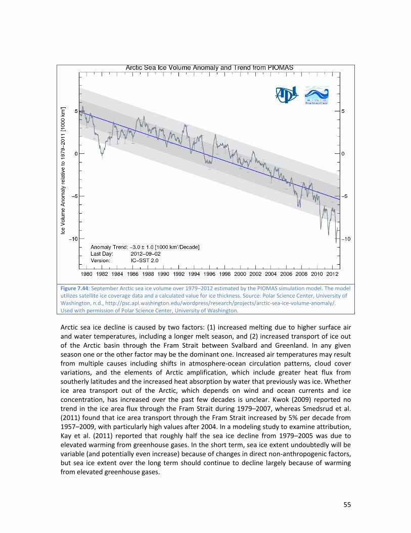
55

Figure 7.44: September Arctic sea ice volume over 1979–2012 estimated by the PIOMAS simulation model. The model utilizes satellite ice coverage data and a calculated value for ice thickness. Source: Polar Science Center, University of Washington, n.d., http://psc.apl.washington.edu/wordpress/research/projects/arctic-sea-ice-volume-anomaly/. Used with permission of Polar Science Center, University of Washington.

Arctic sea ice decline is caused by two factors: (1) increased melting due to higher surface air and water temperatures, including a longer melt season, and (2) increased transport of ice out of the Arctic basin through the Fram Strait between Svalbard and Greenland. In any given season one or the other factor may be the dominant one. Increased air temperatures may result from multiple causes including shifts in atmosphere-ocean circulation patterns, cloud cover variations, and the elements of Arctic amplification, which include greater heat flux from southerly latitudes and the increased heat absorption by water that previously was ice. Whether ice area transport out of the Arctic, which depends on wind and ocean currents and ice concentration, has increased over the past few decades is unclear. Kwok (2009) reported no trend in the ice area flux through the Fram Strait during 1979–2007, whereas Smedsrud et al. (2011) found that ice area transport through the Fram Strait increased by 5% per decade from 1957–2009, with particularly high values after 2004. In a modeling study to examine attribution, Kay et al. (2011) reported that roughly half the sea ice decline from 1979–2005 was due to elevated warming from greenhouse gases. In the short term, sea ice extent undoubtedly will be variable (and potentially even increase) because of changes in direct non-anthropogenic factors, but sea ice extent over the long term should continue to decline largely because of warming from elevated greenhouse gases.

56

Will the Arctic lose its summer ice cover? Recent climate simulations indicate that the Arctic may be free of summer ice as early as 2040 (Holland et al., 2006; Wang and Overland, 2009). A simple extrapolation from the recent observed trajectory for summer sea ice decline, which has outpaced most IPCC model forecasts (Stroeve et al., 2007) (Figure 7.45), indicates that the Arctic will have an ice-free summer by mid-century. Though model projections and extrapolations must be regarded cautiously, given that knowledge of ice-water-atmosphere interactions is far from adequate (see Kwok and Untersteiner, 2011), the extent of Arctic summer sea ice will certainly continue to decline as the Arctic warms. Should (or when) the Arctic become ice free in the summer, it will be the first time for such an event in at least the last 800,000 years (Henson, 2011).

Figure 7.45: Arctic September ice extent (106 km2) from observations (thick red line) and from projections of 13 IPCC models, together with the multi-model mean (dark black line), based on the IPCC “business as usual” A1B Scenario. The blue circle (added by module authors) indicates the 2012 minimum summer (September) ice extent (4.6 x 106 km2). Source: Stroeve et al., 2007. Used with permission of John Wiley & Sons/CCC.

Many writers have suggested that the recession of sea ice will lead to commercial shipping through the Arctic Basin along the Northwest Passage (northern Canadian and Alaskan coast) and the Northeast Passage or Northern Sea Route (northern Russian coast). Although some ice-strengthened ships may indeed traverse the Arctic Basin, more ship traffic will likely be within the Arctic Basin (Figure 7.46) (Smith, 2010; Cressey, 2011). As Smith (2010) points out, the Arctic Ocean will never be completely ice free; it will always freeze in the winter, and in the summer it will always contain patches of ice and icebergs from land-based glaciers at their ocean margin. The “ice-free” summer season will be very short. The lack of port facilities and emergency

57

services, higher insurance rates, adequate charts and navigation services, and the higher cost of ice-strengthened ships will be disincentives (Brigham, 2011; Smith, 2010). As Lawson Brigham (University of Alaska Fairbanks) has pointed out, “The notion that the Arctic Ocean will become a Panama Canal or a Suez Canal is a figment of the media[‘s imagination]” (Cressey, 2011). Ice recession and a lengthening of the “ice-free” summer will certainly spur increases in oil and gas exploitation (Figure 7.47), mining, research, tourism, and ship traffic (within and to the Arctic). Although sea ice recession will create economic opportunities and facilitate easier provisioning of Arctic communities, expansion of ship traffic in the Arctic also poses challenges. There is potential for pollution from ships and other commercial activity, stress on marine mammals due to shipping and sea ice recession, and greater pressures on indigenous cultures. Claims to the seabed and Arctic waters are already under dispute, highlighting the need for international cooperation and new regulations (Brigham, 2011). For indigenous peoples who depend on sea ice as a platform for hunting, the season with reliably stable coastal ice will be shorter and travel across the ice will be more dangerous. Finally, marine mammals dependent on sea ice for aspects of their life history (e.g., hunting, mating, rearing young, travel) will suffer increased stress and increased mortality.

Figure 7.46: Shipping routes (including potential ones) in the Arctic Basin. Source: Hovelsrud et al., 2008. Used with permission of Ecological Society of America/CCC.

58

Figure 7.47: Current oil and gas production areas and potentially known recoverable hydrocarbon reserves in the Arctic. Source: Hovelsrud et al., 2008, modified from AMAP, 1998. Used with permission of Ecological Society of America/CCC.

Arctic Vegetation In the absence of other limiting factors, warming in the Arctic will likely result in range shrinkage for species restricted to the northern part of the tundra zone, northward range extension for the largely boreal species that occupy the southern part of the Arctic, an increase in plant biodiversity (due to entry of new species into the Arctic), and an overall increase in plant productivity. This forecast is based on (1) well-documented relationships between temperature and both biodiversity and plant production (Callaghan et al., 2004, 2005), (2) extensive paleo evidence of treelines that were north of their current positions during the Medieval Warm Period (about A.D. 800–1300) and during parts of what is referred to as the Holocene Thermal Maximum (e.g., MacDonald et al., 2008), and (3) evidence from satellite imagery. Arctic plant species generally are not adapted to the Arctic, which has been ice-free and potentially habitable for a relatively short time; many Arctic plant species originated in cold alpine or upland habitats and have tolerance for lower temperatures (Callaghan et al., 2005) but respond positively to elevated temperatures. Warming in general will be favorable for plant health, growth, and reproduction, though there will be considerable spatial variability. The plants most positively affected will be the boreal species that occupy the southern Arctic; those most

59

negatively affected are likely to be the plant species (relatively few in number) limited to the high north and polar deserts. Growing season length and the length of the snow-free season, in addition to temperatures alone, are key variables that influence vegetation. Both satellite imagery and weather station observations have shown that growing seasons and the duration of the snow-free period are lengthening in most (but not all) Arctic areas. In a recent satellite imagery analysis of phenology changes across the high latitudes (>60oN), Zeng et al. (2012) found that growing season increased on average by 6.3 days over 2000–2010, due mostly to an earlier start of the growing season. Others investigators utilizing satellite imagery for northern high latitudes (see Zeng et al. for summary) have reported increases in growing season length by 0.6–14 days per decade for various time periods during 1981–2008. Weather stations allow an examination of growing season length for Arctic cities and towns over a longer timeframe. For example, the frost-free season in Fairbanks, Alaska increased from 85 to 123 days (45%) over the 20th century (U.S. Global Change Research Program, 2009; Wendler and Shulski, 2009) (Figure 7.48). At the current rate the frost-free season in Fairbanks will increase by another month by 2100, representing a doubling in growing season length in 200 years. Changes in growing season timing and length in the Arctic create the possibility of phenological (timing) mismatches between organisms that respond to temperature cues for seasonal activities (e.g., migration, the timing of fledging) and associated organisms (predators, prey, plant food sources) that rely on light regime cues. Satellite and ground observations indicate the plant biomass and productivity are increasing in the tundra zone. Circumpolar changes in the greenness of tundra vegetation, which is calculated from the Normalized Difference Vegetation Index (NDVI), are being monitored from the satellite record that extends back to 1982. NDVI is correlated with aboveground plant biomass and production. NDVI increased 8% from 1982–2010 for the Arctic overall, though there was considerable spatial and interannual variability (Walker et al., 2011; Walker and Gill, 2011). Time Integrated NDVI (TI-NDVI is the sum of biweekly NDVI over the growing season) patterns are negatively correlated with the springtime sea ice concentration along the coastal Arctic. As summer sea ice has declined, tundra land temperatures and TI-NDVI have increased (Bhatt et al., 2010). Support for the increased greenness from long-term vegetation studies is mixed (Walker et al., 2011). The trends are consistent with observed expansion of shrubs into the tundra zone (e.g., Tape et al., 2006) and the general northward extension of the boreal forest treeline (Callaghan et al., 2005; Hinzman et al., 2005). The extent to which these northward range shifts can be attributed to 20th century warming, however, is not yet clear.

60

Figure 7.48: Length of frost-free season (growing season length) in Fairbanks, Alaska, 1904–2008. Source: G. Juday cited in U.S. Global Change Research Program, 2009. Used with permission of Glenn Juday, University of Alaska Fairbanks.

Simulations of Arctic biome distributions accompanying forecast climate change show the general northward extension of the boreal forest and the compression of the tundra zone as the boreal forest expands and sea level rises (Figure 7.49) (Anisimov et al., 2007; Feng et al., 2011; Sitch et al., 2003). Projections indicate that up to 25% of polar desert may be replaced by tundra and up to 50% of tundra may be replaced by forest depending on the model and the IPCC emissions scenario used. A meta-analysis by Parmesan and Yohe (2003) indicated a poleward shift of plants at an average rate of 6.1 km per decade. Empirical studies (e.g., MacDonald et al., 2008) indicate that the boreal forest will extend northward into the tundra zone at an irregular rate; decadal to centennial time lags will be likely after conditions become suitable for tree establishment and successful reproduction. In some areas unfavorable soil conditions will limit forest establishment. It is also possible that the northern margins of the boreal forest in some areas will be converted to a tundra-steppe, bog, or peatland system depending upon changes in the water regime as permafrost thaws (Callaghan et al., 2005).

61

Figure 7.49: Current and projected (2090–2100) extent of Arctic biomes and sea ice. Source: Anisimov et al., 2007. Used with permission of IPCC.

Extinction Risk of Plant and Animal Species Although the IPPC (2007b) has reported that approximately 20–30% of plant and animal species globally are at risk of extinction if global mean air temperature rises by 1.5–2.5oC (2.7–4.5oF the extinction risk for most terrestrial Arctic species is low (Callaghan et al., 2005; Usher et al., 2005). The species most at risk are the relatively few that are restricted to the high Arctic and polar deserts and potentially some endemic Arctic animal species at risk from more dominant species that extend northward. Range reductions, resulting in the loss of species in some areas, will be the more likely consequence for Arctic species under threat from climate changes and accompanying changes in biotic competition.

Marine Mammals Climate change will influence marine mammals through effects on marine primary productivity, sea ice, other ocean conditions, and the incidence and type of human interactions. The species most sensitive to climate change are those that are regarded as “ice obligate”, which rely on ice for hunting, resting, and breeding (Moore and Huntington, 2008). Other species influenced by sea ice recession and the warming of Arctic waters are those that are “ice associated”, which are associated with ice and adapted to a seasonally ice covered sea, and species that migrate (or are capable of migrating into the Arctic) seasonally into the Arctic Basin (Moore and Huntington, 2008). Laidre et al. (2008) examined the cumulative sensitivity of marine mammals from

62

multiple factors (e.g., site fidelity, sea ice changes, and diet diversity). They reported that the three most sensitive species are the polar bear, narwhale, and hooded seal; the moderately sensitive species are beluga whale, bowhead whale, walrus, spotted seal, ribbon seal, and harp seal. The fitness of animals in both groups is correlated with sea ice extent and is forecast to decline as sea ice extent decreases. Conversely, five whale species (fin, minke, humpback, gray, and killer) are likely to benefit from sea ice recession (Moore and Huntington, 2008) because it will allow increased access to Arctic waters forecast to be increasingly productive. Resilience of marine mammals to sea ice changes due to Arctic warming will likely vary among Arctic regions with populations in some areas benefitting (Moore and Huntington, 2008). All marine mammals will most likely experience increased stress from shipping, pollutants, tourism, and development as sea ice recedes. Polar bears are an Arctic icon, and their status has been used an indicator of climate warming and the health of the Arctic. The Arctic population of polar bears is estimated at 20,000–25,000 and has been divided into 19 separate subpopulations around the Arctic Basin by the International Union for the Conservation of Nature and Natural Resources (IUCN) Polar Bear Specialist Group (PBSG) (Obbard et al., 2010). Knowledge of the size and status of polar bear populations varies among the populations, with relatively good information for some (e.g., longitudinal studies for the populations in Western Hudson Bay and the Southern Beaufort Sea) and poor information for others (Obbard et al., 2010). Because current information for roughly 6 of the 19 populations is poor (Vongraven and Richardson, 2011), it isn’t possible to state with high confidence whether the Arctic polar bear population is stable, declining, or increasing (Figure 7.50). Furthermore, knowledge is lacking about how populations are influenced by the interactions among climate change, contaminants, industrial pressures, prey population size, and hunting pressures (the major cause of bear mortality in many cases; Obbard et al., 2010). Nonetheless, there is compelling evidence that sea ice recession and the lengthening of the ice-free season is having strongly negative effects on the health and size of polar bear populations. The Western Hudson Bay and Southern Beaufort Sea populations, where research has been intensive, serve as potential analogues for how the other Arctic populations may respond to climate change. Polar bears, like walruses and ringed and bearded seals, are an ice-obligate species that depend on sea ice for their survival (Amstrup, 2003; Moore and Huntington, 2008). Polar bears use sea ice as a platform for hunting (primarily seals), movement, mating, and resting, and in some cases denning. Polar bears are most successful at hunting seals from ice that is above the shallow waters of the continental shelf or among islands, where marine productivity and seal populations are higher (Regehr et al., 2010). In the Southern Beaufort Sea most polar bears remain on the sea ice as it recedes during the summer and early fall (Durner et al., 2009; Regehr et al., 2007, 2010); those in Western Hudson Bay, which is ice-free by the end of the summer, come ashore and rely on fat reserves until fall freeze-up (Stirling and Parkinson, 2006; Regehr et al., 2007). In the summer the Southern Beaufort Sea polar bear population has less access to their prey species, which tend to occupy the more productive coastal margin. Bears that are forced to come ashore early or that occupy ice distant from seals are food deprived and at increased risk of starvation. Studies at the Western Hudson Bay and Southern Beaufort sites provide strong evidence that receding sea ice and a lengthening of the ice-free season decreases polar bears’ capture of seals; increases their nutritional stress and energetic costs; and reduces their body condition, breeding

63

success, and survival (Stirling and Parkinson, 2006; Regehr et al., 2007, 2010). The Western Hudson Bay population may be a particularly apt indicator because the bears are at the southern range for the species and because Hudson Bay is ice-free by the end of the summer. In Western Hudson Bay the frequency of bear-human interactions has increased as bears have sought human food sources. Projections of how climate change will affect the total Arctic polar bear population cannot be made with confidence. However, the Western Hudson Bay and the Southern Beaufort findings, the known trends for the 19 populations, and population projections from simulation models are troubling. Currently seven of the Arctic polar bear populations are declining in number, and the decline for two (Western Hudson Bay and Southern Beaufort Sea) have been identified as strongly linked to sea ice recession and a lengthening of the ice-free season (Vongraven and Richardson, 2011). In a recent modeling study Durner et al. (2009) forecast major, extensive losses of polar bear habitat as the Arctic warms. The polar bear may not go extinct during this century, but it likely will be eliminated from much of the Arctic Basin.

Figure 7.50: Status and abundance estimates of polar bears in the 19 subpopulations. Source: Vongraven and Richardson, 2011, updated from Obbard et al., 2010.

64

Natural Resources Marine fisheries Forecasting how climate change will affect fisheries in the Arctic is difficult because many factors influence fish populations. Climate change is only one factor and, with the exception of major ocean temperature oscillations (e.g., ENSO and PDO), not normally the most important factor over a shorter time scale (annual to multidecadal). Other factors that influence fisheries populations and maximum catch potential (sometimes with quick effect) are competition between populations of species, internal population dynamics, contaminants, changes in fisheries regulations and enforcement, and local to global economic factors (Vilhjálmsson et al., 2005). Nonetheless, there is high value in forecasting future fish distributions in the Arctic in response solely to climate change, given that it will experience pronounced climate change for many centuries and because fisheries have high economic importance to Arctic nations. Keep in mind that the maximum wild fisheries catch potential for the world’s oceans has probably been reached (Food and Agriculture Organization [FAO], 2008); many fisheries are fully exploited, over exploited, or in decline (Cheung et al., 2010). Future fisheries distributions and productivity will be influenced by marine primary (phytoplankton) productivity, which is the base of the ocean food chain, and on the thermal ranges for fish species among other factors. Though there is still some disagreement about how climate warming will influence primary production, the growing consensus opinion is that primary production overall for the world’s oceans will decline, primarily because higher ocean temperatures will increase vertical stratification and decrease upwelling of nutrients from deeper waters to the surface waters that contain the phytoplankton (Boyce et al., 2010; Hoegh-Guldberg and Bruno, 2010). However, in the Arctic changes in sea ice currently have a stronger effect on marine productivity (Arrigo et al., 2008). Marine primary production in the Arctic Ocean increased roughly 20% for the 1998–2009 period as sea ice receded and the extent and duration of open water increased (Frey et al., 2011). Arctic fishes, particularly those such as polar cod that depend on the sea edge (a zone of higher primary production), are forecast to decline as the ice retreats and due to competition from southern species. Conversely, commercial fish such as Atlantic cod, herring, and pollock are forecast to benefit as they shift their range northward. In a modeling study that forecast how commercial fisheries would respond to higher ocean temperatures, Cheung et al. (2010) projected large increases in catch potential for the North Atlantic, Bering Sea, and Barents Sea between 2005 and 2055 (Figure 7.51) and decreases in parts of the tropics and subtropics. Under the middle-of-the-road IPCC climate change scenario (A1B), 10-year average catch potentials by 2055 are projected to rise 18–45% for Nordic countries such as Norway, Iceland, and Greenland, and 20% in North Pacific waters off Alaska and the Russian Far East. Norway is forecast to experience the highest increase in catch potential of all countries, with a roughly 45% increase by 2055 relative to 2005. Commercial fisheries industries generally are highly adaptable to environmental change; additionally, Arctic nations have high adaptation capacity because of a rich knowledge base, substantial financial capacity, and generally responsive regulatory agencies (Vilhjálmsson et al., 2005). Although any predictions must be regarded with caution, the commercial fishing industries of the Arctic nations may be among the beneficiaries of climate change.

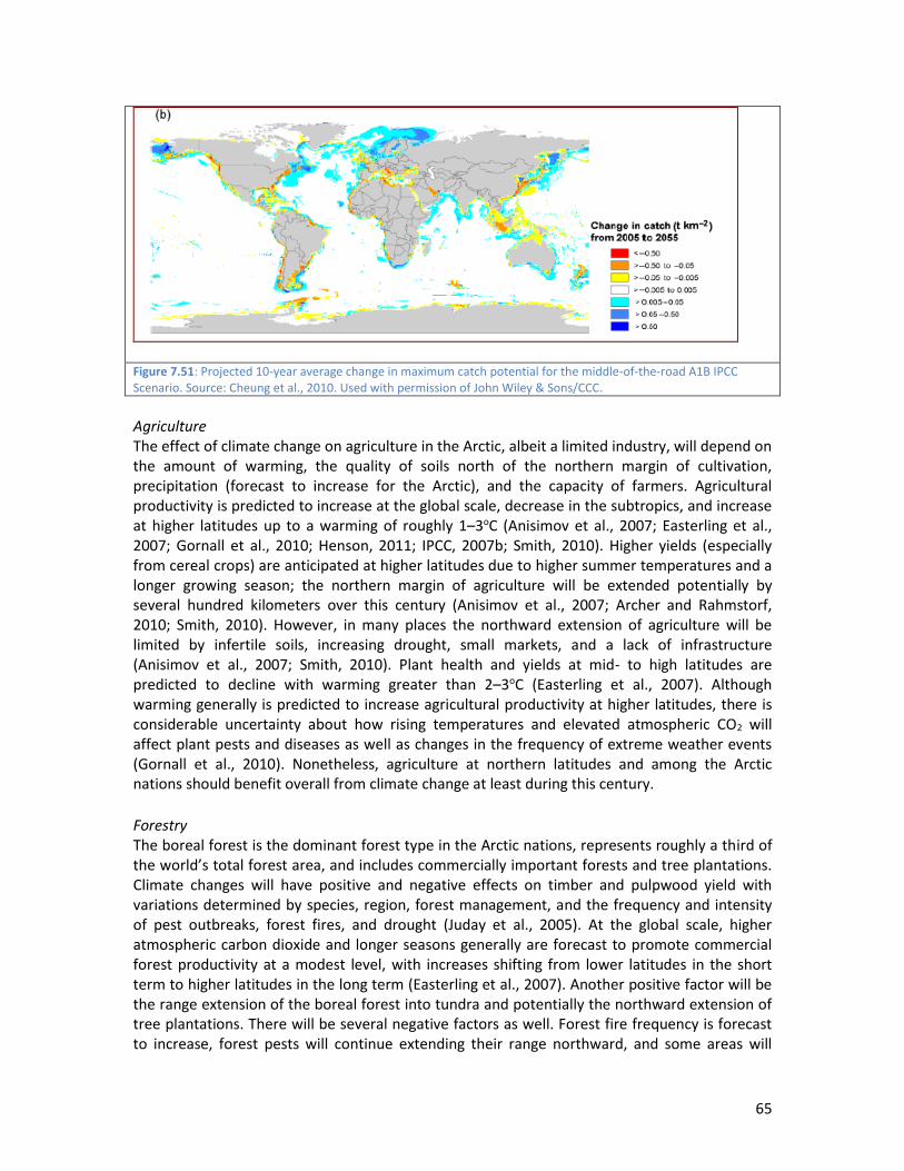
65

Figure 7.51: Projected 10-year average change in maximum catch potential for the middle-of-the-road A1B IPCC Scenario. Source: Cheung et al., 2010. Used with permission of John Wiley & Sons/CCC.

Agriculture The effect of climate change on agriculture in the Arctic, albeit a limited industry, will depend on the amount of warming, the quality of soils north of the northern margin of cultivation, precipitation (forecast to increase for the Arctic), and the capacity of farmers. Agricultural productivity is predicted to increase at the global scale, decrease in the subtropics, and increase at higher latitudes up to a warming of roughly 1–3oC (Anisimov et al., 2007; Easterling et al., 2007; Gornall et al., 2010; Henson, 2011; IPCC, 2007b; Smith, 2010). Higher yields (especially from cereal crops) are anticipated at higher latitudes due to higher summer temperatures and a longer growing season; the northern margin of agriculture will be extended potentially by several hundred kilometers over this century (Anisimov et al., 2007; Archer and Rahmstorf, 2010; Smith, 2010). However, in many places the northward extension of agriculture will be limited by infertile soils, increasing drought, small markets, and a lack of infrastructure (Anisimov et al., 2007; Smith, 2010). Plant health and yields at mid- to high latitudes are predicted to decline with warming greater than 2–3oC (Easterling et al., 2007). Although warming generally is predicted to increase agricultural productivity at higher latitudes, there is considerable uncertainty about how rising temperatures and elevated atmospheric CO2 will affect plant pests and diseases as well as changes in the frequency of extreme weather events (Gornall et al., 2010). Nonetheless, agriculture at northern latitudes and among the Arctic nations should benefit overall from climate change at least during this century.

Forestry The boreal forest is the dominant forest type in the Arctic nations, represents roughly a third of the world’s total forest area, and includes commercially important forests and tree plantations. Climate changes will have positive and negative effects on timber and pulpwood yield with variations determined by species, region, forest management, and the frequency and intensity of pest outbreaks, forest fires, and drought (Juday et al., 2005). At the global scale, higher atmospheric carbon dioxide and longer seasons generally are forecast to promote commercial forest productivity at a modest level, with increases shifting from lower latitudes in the short term to higher latitudes in the long term (Easterling et al., 2007). Another positive factor will be the range extension of the boreal forest into tundra and potentially the northward extension of tree plantations. There will be several negative factors as well. Forest fire frequency is forecast to increase, forest pests will continue extending their range northward, and some areas will

66

experience droughts as increased evapotranspiration (water losses) due to higher temperatures outweighs increased precipitation; the southern portion of the boreal forest is projected to be converted to an open forest-steppe community due to greater water deficits (Flannigan et al., 2005; Juday et al., 2005). How the potential yield of harvestable timber and pulpwood will respond to climate change cannot be forecast with confidence because of the uncertainties of climate forecasts, particularly at the local to regional levels. The amount of warming and plant water availability will remain strongly controlling factors. As with fisheries and agriculture, the timber production response will depend largely on the capability and adaptive capacity of the forestry industry together with fire management practices.

7.10 Conclusions

Until recently the Arctic was viewed as static and unchanging, perhaps because it is remote and far from the public eye. However, that view is at odds with reality. Change is fundamental to the Arctic. The Arctic has in fact experienced greater changes in temperature, vegetation, and ocean surface characteristics than other latitudes in the northern hemisphere for over the past 65 million years (Miller et al., 2010). Now the Arctic is changing rapidly again but this time with the inclusion of considerable human dimensions. The Arctic is no longer unknown to the peoples that live in the populous areas to the south. The satellite images of shrinking Arctic ice have dramatized the astonishing speed with which the Arctic is changing. The Arctic now has great significance to the peoples and nations to the south. In addition to serving as a global indicator of climate change, the Arctic is increasingly important because of the new accessibility to fossil fuel and minerals, the possibilities for increased Arctic shipping, the prospects for tourism, the potential benefits for natural resource industries, and its strategic importance. Climate change is one factor of many that are interrelated and together will change the Arctic in profound ways during this century. The climate changes alone during this century will likely be greater and more rapid than any ever experienced by Arctic inhabitants. Will the changes be good or bad? Change itself is value neutral. Whether the changes are good or bad depends on what is affected, the amount of change, the timeframe, how individuals and governments respond, and your point of view. Certainly there will be some benefits. The Canadian government recently published a report titled “Climate Change Prosperity” which led with the statement, “This is not about coping with climate change, but prospering through it” (National Round Table on the Environment and the Economy, Canada, 2010). Ultimately the potential for Arctic nations and their people to respond to climate change without harm, and potentially to prosper from it, depends on adaptive capacity. Slowing down or reversing human-caused warming, given the lack of collective, international political will to reduce greenhouse gas emissions, no longer seems plausible. The most important requirement for nations to adapt to climate change and potentially prosper from it is wealth. This means not only financial wealth but also wealth with respect to technical expertise, innovation, educational resources, and a trained work force. In this regard the Arctic nations may be among the world’s lucky ones, as the climate warms, because the eight Arctic nations are rich relative to the world average and certainly relative to the subtropics. With increased access to petroleum reserves and the likely production increases in forestry, agriculture, and fisheries, they are likely to get richer, at least in the short term and with a more modest temperature rise.

67

In contrast, the response of the Arctic biological systems will be much more variable. Boreal species will prosper and extend northward, and plant and animal biodiversity plus plant productivity will increase. Conversely, plant and animal species that are endemic to the Arctic will likely experience range reductions and shifts, population decreases, and in perhaps a few cases extinctions. Species at the southern range of the Arctic will extend northward and largely outcompete more northern species. With respect to physical stressors, receding ice extent, though benefitting shipping and commercial fisheries potentially, will negatively affect those ice-obligate and ice associated marine mammals as well as indigenous peoples who depend upon ice as a hunting platform and for transportation. It is hard to identify any benefits from sea level rise, which may be one of the most negative consequences of climate change for coastal towns and cities in the Arctic and worldwide. The wild card for the future is the amount of climate change. Forecasting with confidence the consequences of the upper range of warming possible for the Arctic is far beyond our capability. Undoubtedly, warming at the upper forecast range would severely test not only the Arctic’s biological resources but its nations as well.

Acknowledgements We thank F. S. Chapin, John Walsh, Donald “Skip” Walker, and the University of the Arctic Course Core Revision Team for their highly constructive reviews and Elizabeth Keech for her expert editorial assistance.

References Alaska Climate Research Center, University of Alaska Fairbanks. May 23, 2012. Temperature Change in Alaska. Available at http://climate.gi.alaska.edu/ClimTrends/Change/TempChange.html, accessed November 4, 2012. Alexeev, V. A., Esau, I., Polyakov, I. V., Byam, S. J., and Sorokina, S. 2011. Vertical structure of recent arctic warming from observed data and reanalysis products. Climatic Change 84:295-311. doi:10.1007/s10584-011-0192-8. Alexeev, V. A., Langen, P. L., and Bates, J. R. 2005. Polar amplification of surface warming on an aquaplanet in “ghost forcing” experiments without sea ice feedbacks. Climate Dynamics 24:655-666. Alley, R. B. 2000. The Younger Dryas cold interval as viewed from central Greenland. Quaternary Science Reviews 19:213-226. Alley, R. B., Meese, D. A., Shuman, C. A., Gow, A. J., Taylor, K. C., Grootes, P. M., White, J. W. C., Ram, M., Waddington, E. D., Mayewski, P. A., and Zielinski, G. A. 1993. Abrupt increase in Greenland snow accumulation at the end of the Younger Dryas event. Nature 362:527-529.

68

Amstrup, S. C. 2003. Polar bear, Ursus maritimus. In G. A. Feldhamer, B. C. Thompson, and J. A. Chapman (Eds.), Wild Mammals of North America: Biology, Management, and Conservation (2nd ed.), pp. 587-610. Johns Hopkins University Press, Baltimore, Maryland, USA. Anisimov, O. A., Vaughan, D. G., Callaghan, T. V., Furgal, C., Marchant, H., Prowse, T. D., Vilhjálmsson, H., and Walsh, J. E. 2007. Polar regions (Arctic and Antarctic). In M. L. Parry, O. F. Canziani, J. P. Palutikof, P. J. van der Linden, and C. E. Hanson (Eds.), Climate Change 2007: Impacts, Adaptation and Vulnerability. Contribution of Working Group II to the Fourth Assessment Report of the Intergovernmental Panel on Climate Change, pp. 653-685. Cambridge University Press, Cambridge, UK. Archer, D., and Rahmstorf, S. 2010. The Climate Crisis: An Introduction to Climate Change. Cambridge University Press, Cambridge, UK. Arctic Monitoring Assessment Programme (AMAP). n.d. Geographical Coverage. Available at http://www.amap.no/aboutamap/geocov.htm, accessed October 30, 2012. AMAP. 1998. Assessment Report: Arctic Pollution Issues. Arctic Monitoring and Assessment Programme, Oslo, Norway. Arrigo, K. R., van Dijken, G., and Sudeshna, P. 2008. Impact of shrinking Arctic ice cover on marine primary production. Geophysical Research Letters 35, L19603. doi:10.1029/2008GL035028. Bekryaev, R. V., Polyakov, I. V., and Alexeev, V. A. 2010. Role of polar amplification in long-term surface air temperature variations and modern Arctic warming. Journal of Climate 23:3888-3906. Bhatt, U. S., Walker, D. A., Raynolds, M. K., Comiso, J. C., Epstein, H. E., Jia, G., Gens, R., Pinzon, J. E., Tucker, C. J., Tweedie, C. E., and Webber, P. J. 2010. Circumpolar Arctic tundra vegetation change is linked to sea-ice decline. Earth Interactions 14:1-20. doi: 10.1175/2010EI315.1. Bieniek, P. A., Bhatt, U. S., Rundquist, L. A., Lindsey, S. D., and Zhang, X. D. 2011. Large-Scale Climate Controls of Interior Alaska River Ice Breakup. Journal of Climate 24:286-297. Bindoff, N. L., Willebrand, J., Artale, V., Cazenave, A., Gregory, J., Gulev, S., Hanawa, K., Le Quéré, C., Levitus, S., Nojiri, Y., Shum, C. K., Talley, L. D., and Unnikrishnan, A. 2007. Observations: Oceanic Climate Change and Sea Level. In: S. Solomon, D. Qin, M. Manning, Z. Chen, M. Marquis, K. B. Averyt, M. Tignor, and H. L. Miller (Eds.), Climate Change 2007: The Physical Science Basis. Contribution of Working Group I to the Fourth Assessment Report of the Intergovernmental Panel on Climate Change, pp. 385-432. Cambridge University Press, Cambridge, UK and New York, NY, USA. Bjerknes, J. 1969. Atmospheric teleconnections from the equatorial Pacific. Monthly Weather Review 97:163–172. Boyce, D. G., Lewis, M. R., and Worm, B. 2010. Global phytoplankton decline over the past century. Nature 466:591-596. doi:10.1038/nature09268.

69

Braganza, K., Karoly, D. J., Hirst, A. C., Stott, P., Stouffer, R. J., and Tett, S. F. B. 2004. Simple indices of global climate variability and change Part II: attribution of climate change during the twentieth century. Climate Dynamics 22:823-838. doi:10.1007/s00382-004-0413-1. Brandt, R. E., Warren, S. G., and Clarke, A.D. 2011. A controlled snowmaking experiment testing the relation between black carbon content and reduction of snow albedo. Journal of Geophysical Research 116, D08109. doi:10.1029/2010JD015330. Brigham, L. 2011. Marine protection in the Arctic cannot wait. Nature 478:157. Broecker, W. S. 1975. Climatic Change: Are We on the Brink of a Pronounced Global Warming? Science 189:460-463. Broecker, W. S., Denton G. H., Edwards L. R., Cheng H., Alley R. B., and Putnam, A. E. 2010. Putting the Younger Dryas cold event into context. Quaternary Science Reviews 29:1078-1081. Burroughs, W. J. 2007. Climate Change: A Multidisciplinary Approach (2nd ed.). Cambridge University Press, Cambridge, UK. Callaghan, T. V., Björn, L. O., Chernov, Y. I., Chapin III, F. S., Christensen, T. R., Huntley, B., Ims, R., Johansson, M., Jolly, D., Jonasson, S., Matveyeva, N., Panikov, N., Oechel, W., Shaver, G., Elster, J., Henttonen, H., Laine, K., Taulavuori, K., Taulavuori, E., and Zöckler, C. 2004. Biodiversity, distributions, and adaptations of Arctic Species in the context of environmental change. Ambio 33:404-417. Callaghan, T. V ., Björn, L. O., Chernov, Y. I., Chapin III, F. S., Christensen, T. R., Huntley, B., Ims, R., Johansson, M., Jolly, D., Matveyeva, N. V., Panikov, N., Oechel, W. C., and Shaver, G. R. 2005. Arctic tundra and polar ecosystems. In C. Symon, L. Arris, and B. Heal (Eds.), Arctic Climate Impact Assessment, ACIA, pp. 243-351. Cambridge University Press, Cambridge, UK. Carter, T. R. 2010. Assessing impacts of climate change: an editorial essay. Wiley Interdisciplinary Reviews (WIREs). Climate Change 1: 479-482. Chapman, W. L., and Walsh, J. E. 2007. Simulations of Arctic Temperature and Pressure by Global Coupled Models. Journal of Climate 20:609-632. Cheung, W. L., Lam, V. W. Y., Sarmiento, J. L., Kearney, K., Watson, R., Zeller, D., and Pauly, D. 2010. Large-scale redistribution of maximum fisheries catch potential in the global ocean under climate change. Global Change Biology 16:24-35. doi:10.1111/j.1365-2486.2009.01995x. Christensen, J. H., Hewitson, B., Busuioc, A., Chen, A., Gao, X., Held, I., Jones, R., Kolli, R. K., Kwon, W.-T., Laprise, R., Magaña Rueda, V., Mearns, L., Menéndez, C. G., Räisänen, J., Rinke, A., Sarr, A., and Whetton, P. 2007. Regional climate projections. In S. Solomon, D. Qin, M. Manning, Z. Chen, M. Marquis, K. B. Averyt, M. Tignor and H. L. Miller (Eds.), Climate Change 2007: The Physical Science Basis. Contribution of Working Group I to the Fourth Assessment Report of the Intergovernmental Panel on Climate Change, pp. 847-906. Cambridge University Press, Cambridge, UK and New York, NY, USA.

70

Cook, J. 2010. The Scientific Guide to Global Warming Skepticism. Available at www.skepticalscience.com, accessed January 21, 2013. Cressey, D., 2011. Scientific challenges in the Arctic: Open water. Nature 478:174-177. Dirmeyer, P. A., Niyogi, D., de Noblet-Ducoudré, N., Dickinson, R. E., and Snyder, P. K. 2010. Impacts of land use change on climate. International Journal of Climatology 30:1905–1907. doi: 10.1002/joc.2157. Durner, G. M., Douglas, D. C., Nielson, R. M., Amstrup, S. C., McDonald, T. L., Stirling, I., Mauritzen, M., Born, E. W., Østein, W., DeWeaver, E. D., Serreze, M. C., Belikov, S. E., Holland, M. M., Maslanik, J., Aars, J., Bailey, D. A., and Derocher, A. E. 2009. Predicting 21st-century polar bear habitat distribution from global climate models. Ecological Monographs 79:25-58. Easterling, W. E., Aggarwal, P. K., Batima, P., Brander, K. M., Erda, L., Howden, S. M., Kirilenko, A., Morton, J., Soussana, J.-F., Schmidhuber, J., and Tubiello, F. N. 2007. Food, fibre and forest products. In M. L. Parry, O. F. Canziani, J. P. Palutikof, P. J. van der Linden, and C. E. Hanson (Eds.), Climate Change 2007: Impacts, Adaptation and Vulnerability. Contribution of Working Group II to the Fourth Assessment Report of the Intergovernmental Panel on Climate Change, pp. 273-313. Cambridge University Press, Cambridge, UK. Feng, S., Ho, C.-H., Hu, Q., Oglesby, R. J., Jeong, S.-J., and Kim, B.-M. 2011. Evaluating observed and projected future climate changes for the Arctic using the Köppen-Trewartha climate classification. Climate Dynamics 38:1359-1373. doi:10.1007/s00382-011-1020-6. Feynman, J., and Ruzmaikin, A. 2007. Climate stability and the development of agricultural societies. Climatic Change 84:295-311. doi:10.1007/s10584-007-9248-1. Firestone, R. B., West, A., Kennert, J. P., Becker, L., Bunch, T. E., Revay, Z. S., Schultz, P. H., Belgya, T., Kennert, D. J., Erlandson, J. M., Dickenson, O. J., Goodyear, A. C., Harris, R. S., Howard, G. A., Kloosterman, J. B., Lechler, P., Mayewski, P. A., Montgomery, J., Poreda, R., Darrah, T., Hee, S. S., Que, Smith, A. R., Stich, A., Topping, W., Wittke, J. H., and Wolbach, W. S. 2007. Evidence for an extraterrestrial impact 12,900 years ago that contributed to the megafaunal extinctions and the Younger Dryas cooling. Proceedings of the National Academy of Sciences 104:16016-16021. doi:10.1073/pnas.0706977104. Flannigan, M. D., Logan, K. A., Amiro, B. D., Skinner, W. R., and Stocks, B. J. 2005. Future area burned in Canada. Climatic Change 72:1-16. doi:10.1007/s10584-005-5935-y. Food and Agriculture Organization (FAO). 2008. The State of World Fisheries and Aquaculture (SOFIA). FAO, Rome, Italy.

71

Forster, P., Ramaswamy, V., Artaxo, P., Berntsen, T., Betts, R., Fahey, D. W., Haywood, J., Lean, J., Lowe, D. C., Myhre, G., Nganga, J., Prinn, R., Raga, G., Schulz, M., and Van Dorland, R. 2007. Changes in Atmospheric Constituents and in Radiative Forcing. In S. Solomon, D. Qin, M. Manning, Z. Chen, M. Marquis, K. B. Averyt, M. Tignor and H. L. Miller (Eds.), Climate Change 2007: The Physical Science Basis. Contribution of Working Group I to the Fourth Assessment Report of the Intergovernmental Panel on Climate Change, pp. 129-234. Cambridge University Press, Cambridge, UK and New York, NY, USA. Frey, K. E., Arrigo, K. R., and Gradinger, R. R. 2011. Arctic Ocean Primary Productivity, In J. Richter-Menge, M.O. Jeffries, and J.E. Overland (Eds.), Arctic Report Card: Update for 2011, pp. 69-71. Available at http://www.arctic.noaa.gov/reportcard_previous.html, accessed January 21, 2013. Gessen, K. 2012. Polar Express. The New Yorker, December 24 & 31, pp. 98-117. Gong, D.-Y., and Ho, C.-H. 2002. The Siberian High and climate change over middle to high latitude Asia. Theoretical and Applied Climatology 72:1-9. doi: 10.1007/s007040200008. Gornall, J., Betts, R., Burke, E., Clark, R., Camp, J., Willet, K., and Wiltshire, A. 2010. Implications of climate change for agricultural productivity in the early twenty-first century. Philosophical Transactions of the Royal Society B 365:2973-2989. doi:10.1098/rstb.2010.0158. Griggs, J. A., and Harries, J. E. 2004. Comparison of spectrally resolved outgoing longwave data between 1970 and present. Proceedings of SPIE 5543:164. Hansen, J., and Nazerenko, L. 2004. Soot climate forcing via snow and ice albedos. Proceedings of the National Academy of Sciences 101:423-428. Hansen, J., Nazarenko, L., Ruedy, R., Sato, M., Willis, J., Del Genio, A., Koch, D., Lacis, A., Lo, K., Menon, S., Novakov, T., Perlwitz, J., Russell, G., Schmidt, G. A., and Tausnev, N. 2005. Earth’s Energy Imbalance: Confirmation and Implications. Science 308:1431-1435. Harries, J. E., and Belotti, C. 2010. On the variability of the global net radiative energy balance on the nonequilibrium Earth. Journal of Climate 23:1277-1290. doi:10.1175/2009JCLI2797.1. Harries, J. E., Brindley, H. E., Sagoo, P. J., and Bantges R. J. 2001. Increases in greenhouse forcing inferred from outgoing longwave radiation spectra of the Earth in 1970 and 1997. Nature 410:355-357. Hegerl, G. C., Zwiers, F. W., Braconnot, P., Gillet, N. P., Luo, J. A., Marengo Orsini, N., Nicholls, J. E., and Stott, P. A. 2007. Understanding and attributing climate change. In S. Solomon, D. Qin, M. Manning, Z. Chen, M. Marquis, K. B. Averyt, M. Tignor and H. L. Miller (Eds.), Climate Change 2007: The Physical Science Basis. Contribution of Working Group I to the Fourth Assessment Report of the Intergovernmental Panel on Climate Change, pp. 663-745. Cambridge University Press, Cambridge, UK and New York, NY, USA.

72

Henson, R. 2011. The Rough Guide to Climate Change. Rough Guides, London, UK. Hinzman, L. D., Bettez, N. D., Bolton, R. W., Chapin, F. S., Dyurgerov, M. B., Fastie, C. L., Griffith, B., Hollister, R. D., Hope, A., Huntington, H. P., Jensen, A. M., Jia, G. J., Jorgenson, T., Kane, D. L., Klein, D. R., Kofinas, G., Lynch, A. H., Lloyd, A. H., McGuire, A. D., Nelson, F. E., Oechel, W. C., Osterkamp, T. E., Racine, C. H., Romanovsky, V. E., Stone, R. S., Stow, D. A., Sturm, M., Tweedie, C. E., Vourlitis, G. L., Walker, M. D., Walker, D. A., Webber, P. J., Welker, J. M., Winker, K. S., and Yoshikawa, K. 2005. Evidence and implications of recent climate change in northern Alaska and other Arctic regions. Climatic Change 72:251-298. doi:10.1007/s10584-005-5352-2. Hirdman, D., Burkhart, J. F., Sodemann, H., Eckhardt, S., Jefferson, A., Quinn, P. K., Sharma, S., Ström, J., and Stohl, A. 2010. Long-term trends of black carbon and sulphate aerosol in the Arctic: changes in atmospheric transport and source region emissions. Atmospheric Chemistry and Physics 10:9351-9368. doi:10.5194/acp-10-9351-2010. Hoegh-Guldberg, O., and Bruno, J. F. 2010. The impact of climate change on the world’s marine ecosystems. Science 328:1523-1528. Hoffman, A. J. 2012. Climate Science as Culture War. Stanford Social Innovation Review 10:30-37. Holland, M. M., and Bitz, C. M. 2003. Polar amplification of climate change in the coupled model intercomparison project. Climate Dynamics 21:221-232. Holland, M. M., Bitz, C. M., and Tremblay, B. 2006. Future abrupt reductions in Arctic sea ice. Geophysical Research Letters 33, L23503. doi:10.1029/2006GL028024. Horel, J. D., and Wallace, J. M. 1981. Planetary-scale atmospheric phenomena associated with the Southern Oscillation. Monthly Weather Review 109:813–829. Hovelsrud, G., McKenna, M., and Huntington, H. P. 2008. Marine mammal harvests and other interactions with humans. Ecological Applications 18 (Supplement):S135-S147. International Arctic Science Committee (Lead Author); McGinley, M. (Topic Editor). 2012. Introduction to Arctic Tundra and Polar Desert Ecosystems. In C. J. Cleveland (Ed.), Encyclopedia of Earth (rev.). Environmental Information Coalition, National Council for Science and the Environment, Washington, D.C., USA. Available from http://www.eoearth.org/article/Introduction_to_Arctic_Tundra_and_Polar_Desert_Ecosystems, accessed January 21, 2013. Intergovernmental Panel on Climate Change (IPCC). 2000. IPCC Special Report Emissions Scenarios: Summary for Policy Makers, A Special Report of IPCC Working Group III. Available at www.ipcc.ch/pdf/special-reports/spm/sres-en.pdf, accessed January 21, 2013. IPCC. 2007a. Climate Change 2007: Synthesis Report. Contribution of Working Groups I, II and III to the Fourth Assessment Report of the Intergovernmental Panel on Climate Change [Core Writing Team, Pachauri, R. K., and Reisinger, A. (Eds.)]. IPCC, Geneva, Switzerland.

73

IPCC. 2007b. Summary for Policymakers. In M. L. Parry, O. F. Canziani, J. P. Palutikof, P. J. van der Linden, and C. E. Hanson (Eds.), Climate Change 2007: Impacts, Adaptation and Vulnerability. Contribution of Working Group II to the Fourth Assessment Report of the Intergovernmental Panel on Climate Change, pp. 7-22. Cambridge University Press, Cambridge, UK. Jevrejeva, S., Moore, J. C., and Grinsted, A. 2012. Sea level projections to AD2500 with a new generation of climate change. Global and Planetary Change 80-81:14-20. doi: 10.1016/j.gloplacha.2011.09.006. Jia, G. J., and Epstein, H. E. 2003. Greening of Arctic Alaska, 1981-2001. Geophysical Research Letters 30, 2067. doi: 10.1029/2003GL018268. Juday, G. P., Barber, V., Duffy, P., Linderholm, H., Rupp, S., Sparrow, S., Vaganov, E., and Yarie, J. 2005. Forests, land management, and agriculture. In C. Symon, L. Arris, and B. Heal (Eds.), Arctic Climate Impact Assessment (ACIA), pp. 781-862. Cambridge University Press, Cambridge, UK. Kaufman, D. S., Schneider, D. P., McKay, N. P., Ammann, C. M., Bradley, R. S., Briffa, K. R., Miller, G. H., Otto-Bliesner, B. L., Overpeck, J. T., Vinther, B. M., and Arctic Lakes 2k Project Members. 2009. Recent Warming Reverses Long-Term Arctic Cooling. Science 325:1236-1239. doi:10.1126/science.1173983. Kay, J. E., Holland, M. M., and Jahn, A. 2011. Inter-annual to multi-decadal Arctic ice extent trends in a warming world. Geophysical Research Letters 38, L15708. doi:10.1029/2011GL048008. Kerr, R. 2000. A North Atlantic Climate Pacemaker for the Centuries. Science 288:1984-1985. doi:10.1126/science.288.5473. Kerr, R. A. 2011. Vital details of global warming are eluding forecasters. Science 334:173-174. Kinnard, C., Zdanowicz, C. M., Fisher, D. A., Isaksson, E., de Vernal, A., and Thompson, L. 2011. Reconstructed changes in Arctic sea ice over the past 1,450 years. Nature 479:509-513. doi:10.1038/nature10581. Kinnard, C., Zdanowicz, C. M., Koerner, R. M., and Fisher, D. A. 2008. A changing Arctic seasonal ice zone: Observations from 1880–2003 and possible oceanographic consequences. Geophysical Research Letters 35, L02507. doi:10.1029/2007GL032507. Kuhlbrodt, T., Griesel, A., Montoya, M., Levermann, A., Hofmann, M., and Rahmstorf, S. 2007. On the driving processes of the Atlantic Meridional Overturning Circulation. Review of Geophysics 45, RG2001. doi:10.1029/2004RG000166. Kwok, R. 2009. Outflow of Arctic Ocean Sea Ice into the Greenland and Barents Seas: 1979-2007. Journal of Climate 22:2438-2457. doi:10.1175/2008CLI2819.1. Kwok, R., and Rothrock, D. A. 2009. Decline in Arctic sea ice thickness from submarine and ICESat records: 1958-2008. Geophysical Research Letters 36, L15501. doi:10.1029/2009GL039035.

74

Kwok, R., and Untersteiner, N. 2011. The thinning of Arctic sea ice. Physics Today, April 2011:36-41. Lacis, A. A., Schmidt, G. A., Rind, D., and Ruedy, R. A. 2010. Atmospheric CO2: Principal control knob governing Earth’s temperature. Science 330:356-359. Laidre, K. L., Stirling, I., Lowry, L. F., Wiig, Ø, Heide-Jørgensen, M. P., and Ferguson, S. H. 2008. Quantifying the sensitivity of Arctic marine mammals to climate-induced habitat change. Ecological Applications 18 (Supplement):S97-S125. Lemke, P., Ren, J., Alley, R. B., Allison, I., Carrasco, J., Flato, G., Fujii, Y., Kaser, G., Mote, P., Thomas, R. H., and Zhang, T. 2007. Observations: Changes in Snow, Ice and Frozen Ground. In S. Solomon, S. Qin, M. Manning, Z. Chen, M. Marquis, K. B. Averyt, M. Tignor and H. L. Miller (Eds.), Climate Change 2007: The Physical Science Basis. Contribution of Working Group I to the Fourth Assessment Report of the Intergovernmental Panel on Climate Change, pp. 337-383. Cambridge University Press, Cambridge, UK and New York, NY, USA. Loarie, S. R., Duffy, P. B., Hamilton, H., Asner, G. P., Field, C. B., and Ackerly, D. D. 2010. The velocity of climate change. Nature 462:1052-1055. doi:10.1038/nature08649. Lockwood, M. 2008. Recent changes in solar outputs and the global mean surface temperature. III. Analysis of contributions to global mean air surface temperature rise. Proceedings of the Royal Society A 464:1387-1404. doi:10.1098/rspa.2007.0348. MacDonald, G. M., Kremenetski, K. V., and Beilman, D. W. 2008. Climate change and the northern Russian treeline zone. Philosophical Transactions of the Royal Society B 363:2285-2299. doi:10.1098/rstb.2007.2200. Manabe, S., and Stouffer, R. J. 1980. Sensitivity of a global climate model to an increase of CO2 concentration in the atmosphere. Journal of Geophysical Research 85:5529–5554. McGranahan, G., Balk, D., and Anderson, B. 2007. The rising tide: assessing the risks of climate change and human settlements in low elevation coastal zones. Environment & Urbanization 19: 17-37. doi:10.1177/0956247807076960. Mantua, N. January 2000. The Pacific Decadal Oscillation (PDO). Available at http://jisao.washington.edu/pdo/, accessed November 4, 2012. Mantua, N. J., Hare, S. R., Zhang, Y., Wallace, J. M., and Francis, R. C. 1997. A Pacific interdecadal climate oscillation with impacts on salmon production. Bulletin of the American Meteorological Society 78:1069-1079. McFarlane, N. 2008. Connections between stratospheric ozone and climate: Radiative forcing, climate variability, and change. Atmosphere-Ocean 46:139-158. doi:10.3137/ao.460107.

75

Meehl, G. A., Stocker, T. F., Collins, W. D., Friedlingstein, P., Gaye, A. T., Gregory, J. M., Kitoh, A., Knutti, R., Murphy, J. M., Noda, A., Raper, S. C. B., Watterson, I. G., Weaver, A. J., and Zhao, Z.-C. 2007. Global Climate Projections. In S. Solomon, D. Qin, M. Manning, Z. Chen, M. Marquis, K. B. Averyt, M. Tignor, and H. L. Miller (Eds.), Climate Change 2007: The Physical Science Basis. Contribution of Working Group I to the Fourth Assessment Report of the Intergovernmental Panel on Climate Change, pp. 747-777. Cambridge University Press, Cambridge, UK and New York, NY, USA. Miller, G. H., Brigham-Grette, J., Alley, R. B., Anderson, L., Bauch, H. A., Douglas, M. S. V., Edwards, M. E., Elias, S. A., Finney, B. P., Fitzpatrick, J. J., Funder, S. V., Herbert, T. D., Hinzman, L. D., Kaufman, D. S., MacDonald, G. M., Polyak, L., Robock, A., Serreze, M. C., Smol, J. P., Spielhagen, R., White, J. W. C., Wolfe, A. P., and Wolff, E. W. 2010. Temperature and precipitation history of the Arctic. Quaternary Science Reviews 29:1679-1715. doi:10.1016/j.quascirev.2010.03.001. Min, S.-K., Zhang, X., Zwiers, F. W., and Hegerl, G. C. 2011. Human contribution to more-intense precipitation extremes. Nature 470:378-381. doi:10.1038/nature09763. Mitchell, J. M. 1961. Recent Secular Changes of Global Temperature. Annals of the New York Academy of Sciences 95:235–250. doi:10.1111/j.1749-6632.1961.tb50036.x. Moore, S. E., and Huntington, H. P. 2008. Arctic marine mammals and climate change: impacts and resilience. Ecological Applications 18 (Supplement):S157-S165. National Aeronautics and Space Administration (NASA). n.d. GISS Surface Temperature Analysis. Available at http://data.giss.nasa.gov/gistemp/maps, accessed November 1, 2012. NASA. May 4, 2012. CERES TRMM Pictures. Available at http://ceres.larc.nasa.gov/trmm_ceres.php, accessed November 4, 2012. NASA, Earth Observatory. n.d. Global Temperatures. Available at http://earthobservatory.nasa.gov/Features/WorldOfChange/decadaltemp.php, accessed November 4, 2012. National Oceanic and Atmospheric Administration (NOAA). n.d. Arctic Change, Climate Indicators–Arctic Oscillation. Available at http://www.arctic.noaa.gov/detect/climate-ao.shtml, accessed November 4, 2012. NOAA, Earth System Research Laboratory. n.d. Trends in Atmospheric Carbon Dioxide. Available

at http://www.esrl.noaa.gov/gmd/ccgg/trends/#mlo, accessed November 1, 2012. NOAA, National Climatic Data Center. December 2012. State of the Climate: Global Analysis for Annual 2012. Available at http://www.ncdc.noaa.gov/sotc/global/2012/13, accessed February 16, 2013.

76

NOAA, National Weather Service, Climate Prediction Center. December 9, 2005. Warm (El Niño/Southern Oscillation – ENSO) Episodes in the Tropical Pacific. Available at http://www.cpc.ncep.noaa.gov/products/analysis_monitoring/impacts/warm_impacts.shtml, accessed November 4, 2012. NOAA, National Weather Service, Climate Prediction Center. December 12, 2005. Arctic Oscillation (AO). Available at www.cpc.ncep.noaa.gov/products/precip/CWlink/daily_ao_index/ao.loading.shtml, accessed November 4, 2012. National Park Service. October 29, 2012. What is Climate Change? Available at http://www.nps.gov/grba/naturescience/what-is-climate-change.htm, accessed November 1, 2012. National Research Council (NRC). 2002. Abrupt Climate Change: Inevitable Surprises. National Academy Press, Washington, D.C., USA. National Research Council (NRC). 2003. Cumulative Environmental Effects of Oil and Gas Activities on Alaska's North Slope. Committee on the Cumulative Environmental Effects of Oil and Gas Activities on Alaska's North Slope. National Academy Press, Washington, D.C., USA. National Round Table on the Environment and the Economy, Canada. 2010. Degrees of Change: Climate Warming and the Stakes for Canada. Ottawa, Canada, NRTEE. National Snow and Ice Data Center (NSIDC). 2011. Arctic Sea Ice New and Analysis. Available at http://nsidc.org/arcticseaicenews/2011/10/summer-2011-arctic-sea-ice-near-record-lows/, accessed January 20, 2013. National Snow and Ice Data Center (NSIDC). 2012a. Arctic Sea Ice News and Analysis, Monthly Archives: October 2012. Available at http://nsidc.org/arcticseaicenews/2012/10/, accessed January 20, 2013. National Snow and Ice Data Center (NSIDC). 2012b. Arctic Sea Ice News and Analysis, Monthly Archives: September 2012. Available at http://nsidc.org/arcticseaicenews/2012/09/, accessed November 6, 2012. Obbard, M. E., Thiemann, G. W., Peacock, E., and DeBruyn, E. (Eds.). 2010. Polar Bears: Proceedings of the 15th Working Group Meeting of the IUCN/SSC Polar Bear Specialist Group, Copenhagen, Denmark, 29 June – 3 July 2009. Gland, Switzerland and Cambridge, UK: IUCN. Panagiotopoulos, F., Shahgedanova, M., Hannachi, A., and Stephenson, D. B. 2005. Observed Trends and Teleconnections of the Siberian High: A Recently Declining Center of Action. Journal of Climate 18:1411-1422. Papineau, J. M., 2001. Wintertime temperature anomalies in Alaska correlated with ENSO and PDO. International Journal of Climatology 21:1577-1592.

77

Parmesan, C., and Yohe, G. 2003. A globally coherent fingerprint of climate change impacts across natural systems. Nature 421:37-42. Past Global Changes (PAGES). 2002. Rapid Climate Change, Central Greenland Climate. Available at http://www.pages.unibe.ch/products/ppt-slides, accessed November 1, 2012. Polar Science Center, University of Washington. n.d. Arctic Sea Ice Volume Anomaly, version 2. Available at http://psc.apl.washington.edu/wordpress/research/projects/arctic-sea-ice-volume-anomaly/, accessed November 6, 2012. Polyak, L., Allen, R. B., Andrews, J. T., Brigham-Grette, J., Cronin, T. M., Darby, D. A., Dyke, A. S., Fitzpatrick, J. J., Funder, S., Holland, M., Jennings, A. E., Miller, G. H., O’Regan, M., Savelle, J., Serreze, M., St. John, K., White, J. W. C., and Wolff, E., 2010. History of sea ice in the Arctic. Quaternary Science Reviews 29:1757-1778. Polyakov, I. V., Alekseev, G., Bekryaev, R., Bhatt, U. S., Colony, R., Johnson, M., Karklin, V., Makshtas, A., Walsh, D., and Yulin, A. 2002. Observationally-based assessment of polar amplification of global warming. Geophysical Research Letters 29:1878. doi:10.1029/2001GL011111. Polyakov, I. V., Bhatt, U. S., Simmons, H. L., Walsh, D., Walsh, J. E., and Zhang, X. 2005. Multidecadal Variability of North Atlantic Temperature and Salinity during the Twentieth Century. Journal of Climate 18:4562-4581. Rahmstorf, S. 2007. A semi-empirical approach to projecting future sea-level rise. Science 315:368-370. Ramaswamy, V., Schwarzkopf, M. D., Randel, W. J., Santer, B. D., Soden, B. J., and Stenchikov, G. L. 2006. Anthropogenic and Natural Influences in the Evolution of Lower Stratospheric Cooling. Science 311:1138-1141. doi:10.1126/science.1122587. Regehr, E. V., Hunter, C. M., Caswell, H., Amstrup, S. C., and Stirling, I. 2010. Survival and breeding of polar bears in the southern Beaufort Sea in relation to sea ice. Journal of Animal Ecology 79:117-127. doi: 10.1111/j.1365-2656.2009.01603.x. Regehr, E. V., Lunn, N. J., Amstrup, S. C., and Stirling, I. 2007. Effects of earlier sea ice breakup on survival and population size in Western Hudson Bay. Journal of Wildlife Management 71:2673-2683. doi: 10.2193/2006-180. Rignot, E., Box, J. E., Burgess, E., and Hanna, E. 2008. Mass balance of the Greenland Ice Sheet from 1958 to 2007. Geophysical Research Letters 35, L20502. doi:10.1029/2008GL035417. Rignot, E., and Kanagaratnam, P. 2006. Changes in the velocity structure of the Greenland Ice Sheet. Science 311:986-990. doi:10.1126/Science.1121381. Rogers, J. C., and van Loon, H. 1979. The Seesaw in Winter Temperatures between Greenland and Northern Europe. Part II: Some Oceanic and Atmospheric Effects in Middle and High Latitudes. Monthly Weather Review 107:509-519.

78

Ruddiman, W. E. 2008. Earth’s Climate (2nd ed.). W. H. Freeman and Company, New York, NY, USA. Schneider, S. H., 1975. On the Carbon Dioxide–Climate Confusion. Journal of the Atmospheric Sciences 32:2060–2066. doi: http://dx.doi.org/10.1175/1520-0469(1975)032<2060:OTCDC>2.0.CO;2 Schwarzkopf, M. D., and Ramaswamy, V. 2002. Effects of changes in well-mixed gases and ozone on stratospheric seasonal temperatures. Geophysical Research Letters 29(24):2184. doi:10.1029/2002GL015759. Schweiger, A., Lindsay, R., Zhang, J., Steele, M., Stern, H., and Kwok, R. 2011. Uncertainty in modeled Arctic sea ice volume. Journal of Geophysical Research 116:C00D06. doi:10.1029/2011JC007084. Serreze, M. C., and Barry, R. G. 2005. The Arctic Climate System. Cambridge University Press, Cambridge, UK. Serreze, M. C., and Barry, R. G. 2011. Processes and impacts of Arctic amplification. Global and Planetary Change 77:85-96. doi:10.1016/j.gloplacha.2011.03.004. Severinghaus, J. P., Sowers, T., Brook, E. J., Alley, R. B., and Bender, M. L. 1998. Timing of abrupt climate change at the end of the Younger Dryas interval from thermally fractionated gases in polar ice. Nature 391:141-146. Sitch, S. B., Smith, B., Prentice, I. C., Arneth, A., Bondeau, A., Cramer, W., Kaplan, J. O., Levis, S., Lucht, W., Sykes, M. T., Thonicke, K., Venevsky, S. 2003. Evaluation of ecosystem dynamics, plant geography and terrestrial carbon cycling in the LPJ dynamics global vegetation model. Global Change Biology 9:161-185. Smedsrud, L. H., Sirevaag, A., Kloster, K., Sorteberg, A., and Sandven, S. 2011. Recent wind driven high sea ice area export in the Fram Strait contributes to Arctic sea ice decline. The Cryosphere 5:821-829. doi:10.5194/tc-5-821-2011. Smith, L. 2010. The World in 2050: Four Forces Shaping Civilization's Northern Future. Dutton/ Penguin, New York, NY, USA. Solomon, S., Qin, D., Manning, M., Alley, R. B., Berntsen, T., Bindoff, N. L., Chen, Z., Chidthaisong, A., Gregory, J. M., Hegerl, G. C., Heimann, M., Hewitson, B., Hoskins, B. J., Joos, F., Jouzel, J., Kattsov, V., Lohmann, U., Matsuno, T., Molina, M., Nicholls, N., Overpeck, J., Raga, G., Ramaswamy, V., Ren, J., Rusticucci, M., Somerville, R., Stocker, T. F., Whetton, P., Wood, R. A., and Wratt, D. 2007. Technical Summary. In S. Solomon, D. Qin, M. Manning, Z. Chen, M. Marquis, K. B. Averyt, M. Tignor, and H. L. Miller (Eds.), Climate Change 2007: The Physical Science Basis. Contribution of Working Group I to the Fourth Assessment Report of the Intergovernmental Panel on Climate Change, pp. 19-91. Cambridge University Press, Cambridge, UK and New York, NY, USA.

79

Stirling, I., and Parkinson, C. L. 2006. Possible effects of climate warming on selected populations of Polar Bears (Ursus maritimus) in the Canadian Arctic. Arctic 59:261-275. Stott, P. A., Gillett, N. P., Hegerl, G. C., Karoly, D. J., Stone, D. A., Zhang, X., and Zwiers, F. 2010. Detection and attribution of climate change: a regional perspective. WIREs Climate Change 1:192-211. doi:10.1002/wcc.34. Stroeve, J., Holland, M. M., Meier, W., Scambos, T., and Serreze, M. 2007. Arctic sea ice decline: Faster than forecast. Geophysical Research Letters 34, L09501. doi:10.1029/2007GL029703. Tanaka, H. L., and Tokinaga, H. 2002. Baroclinic instability in high latitudes induced by polar vortex: A connection to the Arctic Oscillation. Journal of the Atmospheric Sciences 59:69-82. Tape, K., Sturm, M., and Racine, C. 2006. The evidence for shrub expansion in Northern Alaska and the Pan-Arctic. Global Change Biology 12:686-702. Tett, S. F. B., Jones, G. S., Stott, P. A., Hill, D. C., Mitchell, J. F. B., Allen, M. R., Ingram, W. J., Johns, T. C., Johnson, C. E., Jones, A., Roberts, D. L., Sexton, D. M. H., and Woodage, M. J. 2002. Estimation of natural and anthropogenic contributions to twentieth century temperature change. Journal of Geophysical Research 107:10-1 to 10-24. doi:10.1029/2000JD000028. Thompson, D. W. J., and Wallace, J. M. 1998. The Arctic Oscillation signature in the wintertime geopotential height and temperature fields. Geophysical Research Letters 25:1297-1300. Trenberth, K. E. 2012. The IPCC Process. Available at http://www.cgd.ucar.edu/cas/trenbert.html, accessed January 22, 2013. Trenberth, K. E., and Fasullo, J. T. 2010. Tracking Earth’s Energy. Science 328:316-317. Trenberth, K. E., Fasullo, J. T., and Kiehl, J. 2009. Earth’s Global Energy Budget. Bulletin of the American Meteorological Society 90:311-323. Trenberth, K. E., Houghton, J. T., and Meira Filho, L. G. 1996. The Climate System: an overview. In J. T. Houghton, L. G. Meira Filho, B. A. Callander, N. Harris, A. Kattenberg, and K. Maskell (Eds.), Climate Change 1995, The Science of Climate Change, Contribution of Working Group I to the Second Assessment Report of the Intergovernmental Panel on Climate Change, pp. 51-64. Cambridge University Press, Cambridge, UK. Trenberth, K. E., Jones, P. D., Ambenje, P., Bojariu, R., Easterling, D., Klein Tank, A., Parker, D., Rahimzadeh, F., Renwick, J. A., Rusticucci, M., Soden, B., and Zhai, P. 2007. Observations: Surface and atmospheric climate change. In S. Solomon, D. Qin, M. Manning, Z. Chen, M. Marquis, K. B. Averyt, M. Tignor, and H. L. Miller (Eds.), Climate Change 2007: The Physical Science Basis. Contribution of Working Group I to the Fourth Assessment Report of the Intergovernmental Panel on Climate Change, pp. 235-336. Cambridge University Press, Cambridge, UK and New York, NY, USA. Trenberth, K. E., and Paolino, D. A. 1980. The Northern Hemisphere sea-level pressure data set: Trends, errors, and discontinuities. Monthly Weather Review 108:855–872.

80

Truffer, M., and Fahnestock, M. 2007. Rethinking Ice Sheet Time Scales. Science 315:1508-1510. doi:10.1126/science.1140469. Uherek, E. 2006. Upper Atmosphere. ESPERE. Available at http://www.atmosphere.mpg.de/enid/20c.html, accessed April 2, 2011. University Corporation for Atmospheric Research (UCAR). 2012. Digital Image Library. Available at www.fin.ucar.edu/netpub/server.np?findandsite=imagelibraryandcatalog=catalogandtemplate=detail.npandfield=itemidandop=matchesandvalue=3352, accessed November 5, 2012. U. S. Global Change Research Program. 2009. Global Climate Change Impacts in the United States, Karl, T. R., Melillo, J. M., and Peterson, T. C., (Eds.). Cambridge University Press, Cambridge, UK. Usher, M. B., Callaghan, T. V., Gilchrist, G., Heal, B., Juday, G. P., Loeng, H., Muir, M. A. K., and Prestrud, P. 2005. Principles of Conserving the Arctic’s Biodiversity. In C. Symon, L. Arris, and B. Heal (Eds.), Arctic Climate Impact Assessment, ACIA, pp. 539-596, Cambridge University Press, Cambridge, UK. van der Linden, P., and Mitchell, J. F. B. (Eds.). 2009. ENSEMBLES: Climate Change and Its Impacts: Summary of Research and Results from the ENSEMBLES Project. Met Office Hadley Centre, Exeter, UK. van Loon, H., and Rogers, J. C. 1978. The Seesaw in Winter Temperatures between Greenland and Northern Europe. Part I: General Description. Monthly Weather Review 106:296-310.

Vilhjálmsson, H., Hoel, A. H., Agnarsson, S., Arnason, R., Carscadden, J. E., Eide, A., Fluharty, D., Hønneland, G., Hvingel, C., Jakobsson, J., Lilly, G., Nakken, O., Radchenko, V., Ramstad, S., Schrank, W., Vestergaard, N., and Wilderbuer, T. 2005. Fisheries and Aquaculture. In C. Symon, L. Arris, and B. Heal (Eds.), Arctic Climate Impact Assessment (ACIA), pp. 691-780. Cambridge University Press, Cambridge, UK.

Vongraven, D., and Richardson, E. 2011. Biodiversity–Status and Trends of Polar Bears. In J. Richter-Menge, M. O. Jeffries, and J. E. Overland (Eds.), Arctic Report Card: Update for 2011, pp. 75-78. Available at http://www.arctic.noaa.gov/reportcard_previous.html, accessed January 21, 2013.

Walker, D. A., Bhatt, U. S., Callaghan, T. V., Comiso, J. C., Epstein, H. E., Forbes, B. C., Gill, M., Gould, W. A., Henry, G. H. R., Jia, G. J., Kokelj, S. V., Lantz, T. C., Oberbauer, S. F., Pinzon, J. E., Raynolds, M. K., Shaver, G. R., Tucker, C. J., Tweedie, C. E., and Webber, P. J. 2011. Vegetation. In J. Richter-Menge, M. O. Jeffries, and J. E. Overland (Eds.), Arctic Report Card: Update for 2011, pp. 89-95. Available at http://www.arctic.noaa.gov/reportcard_previous.html, accessed January 21, 2013.

81

Walker, D. A., and Gill, M. 2011. Terrestrial Ecosystems Summary. 2011. In J. Richter-Menge, M. O. Jeffries, and J. E. Overland (Eds.), Arctic Report Card: Update for 2011, p. 88. Available at http://www.arctic.noaa.gov/reportcard_previous.html, accessed January 21, 2013. Walker, G. T. 1924. Correlation in seasonal variations of weather, IX: A further study of world weather (World Weather II). Memoirs of the Indian Meteorological Department 24:275-332. Walker, G. T., and Bliss, E. W. 1932. World Weather V. Memoirs of the Royal Meteorological Society 4:53-84.

Wang, K., and Liang, S. 2009. Global atmospheric downward longwave radiation over land surface under all-sky conditions from 1973 to 2008. Journal of Geophysical Research 114, D19101. doi:10.1029/2009JD011800. Wang, M., and Overland, J. E. 2009. A sea ice free summer Arctic within 30 years? Geophysical Research Letters 36, L07502. doi:10.1029/2009GL037820. Weiler, S. C., Keller, J. K., and Olex, C. 2012. Personality type difference between Ph.D. climate researchers and the general public: Implications for effective communication. Climatic Change 112:233-242. doi:10.1007/s10584-011-0205-7. Wendler, G., and Shulski, M. 2009. A Century of Climate Change for Fairbanks, Alaska. Arctic 62:295-300. Wigley, T. M. L., Ramaswamy, V., Christy, J. R., Lanzante, J. R., Mears, C. A., Santer, B. D., and Folland, C. K. 2006. Executive Summary in Temperature Trends in the Lower Atmosphere: Steps for Understanding and Reconciling Differences. In T. R. Karl, S. J. Hassol, C. D. Miller, and W. L. Murray (Eds.), A Report by the Climate Change Science Program and the Subcommittee on Global Change Research, pp. 1-14. Washington, D.C., USA. Woodhouse, C. A., and Overpeck, J. T. 1998. Two thousand years of drought variability in the central United States. Bulletin of the American Meteorological Society 79:2693-2714. Zeng, H., Jia, G., and Epstein, H. 2012. Recent changes in phenology over the northern high latitudes detected from multi-satellite data. Environmental Research Letters 6. doi:10.1088/1748-9326/6/4/045508.

Appendices

APPENDIX A. ACTIVITY: IDENTIFY HOW ANNUAL AND WINTER TEMPERATURE AND PRECIPITATION IN A TOWN OR CITY OF YOUR CHOICE HAVE CHANGED OVER THE PAST FEW DECADES.

Tasks 1. Collect annual and winter (December through February) temperature and precipitation data

for the past 50 years (or longer if the data are available) and plot the data over time for

82

each. You should produce four graphs. Next graph the linear trends; you can use packaged software such as Excel.

2. Assess changes over the past 50 years, including the trends (positive or negative), any changes in variability (the amount of departure from the trends), and any abrupt changes.

3. Compare the four graphs and determine if there are similarities or differences. 4. Seek out 3–4 people who have lived in the town or city for several decades or longer and ask

them whether they think climate has changed or not changed during that time. Ask them if they think winters have changed. Next show them your time series analysis and discuss with them any differences or similarities between their perception of overall climate and winters and the record. If there are differences, discuss why their perceptions may be different from the record.

Example: Download monthly average temperature at http://climate.gi.alaska.edu/Climate/Location/TimeSeries/Data/faiT and precipitation data at http://climate.gi.alaska.edu/Climate/Location/TimeSeries/Data/faiP for Fairbanks, Alaska, from the Alaska Climate Research Center web page for the period 1930–2010. Convert to metric units and plot the data. The plots for Fairbanks’s annual average temperature and precipitation are shown in Figure A.1. Fairbanks’s air temperature displays a warming trend of 1.7 ˚C over the 81 years while the precipitation has decreased 0.43 cm over 81 years. The temperature trend is relatively large compared to the long-term annual average temperature of -3˚C. The precipitation trend is only 1.5% of the long-term mean annual precipitation of 28 cm, making it a relatively weak trend. Temperature and precipitation both display large interannual to decadal fluctuations, so one has to exercise caution when discussing trends, particularly over short time periods.

Figure A.1: The 1930–2010 Fairbanks annual mean air temperature (top left) and precipitation (bottom left) and Fairbanks winter (NDJFM) mean air temperature (top right) and precipitation (bottom right) in oC and cm of water equivalent, respectively.

83

APPENDIX B. SOURCES OF CLIMATE DATA.

Climate data are publically available from a variety of sources on the Web. As you download data or ask for access to data, it is always critical that you have some basic understanding of how the data were collected, the units of the measurements, and the magnitude of the errors. Knowing the basic facts about the data will give you more confidence in your analysis and interpretation. In climate research or any research for that matter, it is necessary to question your data quality, your analysis, and your interpretation. The following tables provide links to climate data around the world with some guidance on the types of data. The sites listed here provide most of their data free of charge for educational activities. There is no simple one-stop-shop for climate data and the best available data set is often a changing target. You must exercise your judgment when you use available data. This is by no means a complete list and is meant to provide students with a starting point to become familiar with the types of climate data that are available for analysis. Table B.1: Climate data sources.

World Meteorological Organization (WMO)

http://www.wmo.int/pages/prog/gcos/

Under “Observing Systems and Data,” the World Meteorological Organization through the Global Climate Observing System (WMO GCOS) provides links for surface and upper air stations, chemical composition, ocean, and terrestrial data sets.

U.S. National Climatic Data Center (NCDC)

http://www.ncdc.noaa.gov/oa/ncdc.html

The U.S. National Climatic Data Center provides access to a variety of climate data sets including atmosphere, ocean, and terrestrial parts of the system.

University of Wyoming, U.S.

http://weather.uwyo.edu/upperair/sounding.html

The University of Wyoming, Department of Atmospheric Sciences in the U.S. has upper air data for the entire globe available in a graphical interface. Stations throughout the Arctic are available. This is more a weather page, and it is not easy to download long time series.

National Climate Archives

Country-specific links

Various countries have national climate archives where data for your locality is available. You will need to search the Internet or contact your local governmental office to obtain access to this data.

UK Met Office Hadley Center

http://www.metoffice.gov.uk/hadobs/

This site contains sea surface temperature, sea level pressure, and surface air temperatures on monthly time scales. Some higher temporal resolution is available.

U.S. National Oceanic and Atmospheric Administration (NOAA)

http://www.ncdc.noaa.gov/temp-and-precip/ghcn-gridded-products.php#data

This site contains monthly temperature and precipitation anomalies over land from 1900 to present based on station data and gridded for a 5o x 5o latitude/longitude grid.

84

Table B.2: Climate indices sources. Climate indices describe large-scale variability in climate and help to link changes in different regions.

U.S. National Oceanic and Atmospheric Administration (NOAA)

http://www.esrl.noaa.gov/psd/data/climateindices/list/

This page provides a fairly comprehensive list of updated climate indices in an easy-to-use format. This is a good place to start looking for an index.

University Corporation for Atmospheric Research, U.S.

http://www.cgd.ucar.edu/cas/jhurrell/indices.html

This page offers clear explanations and a choice of seasonal indices of the North Atlantic Oscillation and the Northern Annular Mode (Arctic Oscillation).

U.S. National Oceanic and Atmospheric Administration (NOAA)

http://www.cpc.ncep.noaa.gov/data/indices/index.shtml

This site offers a variety of climate teleconnection indices for typically shorter time scales than above sites.

Table B.3: Paleoclimate data sources.

U.S. National Oceanic and Atmospheric Administration (NOAA)

http://www.ncdc.noaa.gov/paleo/globalwarming/proxydata.html

This NOAA Paleoclimatology site provides an excellent overview of key paleoclimate data and links to the data.

University of Copenhagen

http://www.iceandclimate.nbi.ku.dk/data/

Ice core time series can be requested from this website.

APPENDIX C. SOURCES OF CLIMATE CHANGE INFORMATION (EXTRACTED AND REVISED FROM THE CLIMATE CHANGE MODULE IN BCS 100)

Climate change is now a daily topic in the popular media (e.g., websites, television, radio, blogs, and newspapers). The media often report stories that raise the level of controversy surrounding a topic (e.g., is global warming caused by humans?) without providing an informed analysis of the scientific evidence. Keeping up with the nuances of scientific disagreements about climate change is beyond the capability or interest of most laypeople. In most cases people decide what to “believe,” or to side with one expert or another, based on their assessment of the expert’s credibility and whether the information appears to be sound and is aligned with their value system. How can the non-scientist decide what information and sources are trustworthy? Here are some recommendations about different sources of information:

The media: Information from the media can be suspect because the goal of journalists and reporters, with some exceptions, is not to “get the science right” but to publish a story that is newsworthy. When reading a media article you should consider the background and institutional affiliations of any scientists who are quoted. Information about the professional credentials and research background of any scientist should be

85

available via a Web search. Especially relevant is whether a quoted scientist actually conducts climate science research.

Books: The reliability of information about climate science in books depends in part on whether the books are for a popular or academic audience. Popular books often take one point of view rather than presenting a dispassionate objective examination of scientific facts and principles. Academic books predominantly are accurate, but may not be easily understood without a background in the discipline. Some recent academic books (e.g., Archer and Rahmstorf, 2010) provide a superb grounding in climate change science and can be readily understood by a non-scientist. For either type of book (popular or academic) consider the publication date. The field of climate science is changing quickly. The basics of climate science haven’t changed for decades, but knowledge about climate change (given the various factors that cause it and are affected by it) is growing and changing rapidly. Keep in mind that authors are paid by publishers, whose goal is to sell books.

Scientific articles: These are generally the most reliable sources of information on climate change, though they are generally too advanced for someone without a science background or even for scientists outside the climate science discipline. Some journals (e.g., Science and Nature) provide in each issue a short profile, written in less technical language, of scientific articles in the issue that are regarded as having highest scientific impact.

Websites: Websites not surprisingly can be problematic. The quality varies greatly and depends on who or what organization produces the site. Some, particularly websites from government agencies (e.g., NASA, World Meteorological Organization, Environment Canada, United Nations Environment Program) are excellent. Other websites contain erroneous and sometimes biased information (intentional or not). In all cases consider if a website appears objective or politically motivated, and if information sources are fully referenced.

Although judgment is always required in assessing the reliability of information, the guidelines above should help. What are the best sources of information about climate change? Below appear two of the most comprehensive and reliable sources that have gone through critical peer review and represent the consensus view of the most outstanding scientists across the globe:

Intergovernmental Panel on Climate Change (IPCC): The IPCC developed from the World Meteorological Organization and has released regular assessments on climate change and its impacts since 1990. The IPCC released its Fourth Assessment Report in 2007 and is now working on its Fifth Assessment. IPCC reports represent the most current, vetted state of knowledge and include extensive citations from the peer-reviewed literature. A notable feature of the more recent IPCC reports is that they provide the degree of uncertainty (virtually certain to exceptionally unlikely) about findings and forecasts. All IPCC reports (including figures) are freely available and can be downloaded from the IPCC website (www.ipcc.ch). Importantly the IPCC does not conduct research, but instead evaluates and summarizes the scientific literature. The working group that summarized the physical basis for climate change (Working Group 1, WG1) in the most recent IPCC Assessment Report (the fourth, abbreviated as AR4) included over 450 lead authors, 800 contributing authors, and over 2,500 reviewers from 130 countries; the authors and reviewers are

86

international leaders in climate change science and include some that identify themselves as climate change “skeptics” (Trenberth, 2012). All comments from reviewers of the AR4 WG1 report, the Technical Summary, and the Summary for Policy Makers are archived at Harvard University and publically available (Trenberth, 2012).

Arctic Climate Impact Assessment (ACIA): The ACIA report, published in 2005, is the first comprehensive and multi-disciplinary assessment of climate change and its impacts in the Arctic. The report includes not only the record of climate change but also effects on natural resources (fisheries, forestry, wildlife) and indigenous peoples. The ACIA report is freely downloadable from the ACIA website (www.acia.uaf.edu).

Another excellent and recent report, though not having gone through the rigorous IPCC review process, is the Climate Change Science Compendium 2009 authored by the United Nations Environment Program (www.unep.org/compendium2009/). The report summarizes roughly 400 reports from the peer-reviewed scientific literature and research institutions published since the deadline of research reports considered for the IPCC Fourth Assessment. In addition to the IPCC, ACIA, and UNEP resources, many government and university websites are excellent sources of information on climate change. A selection of recommended sites is below: Table C.1: Selection of recommended government and university climate change websites.

Organization Website

GRID – Arendale, Norway, United Nations Environment Program (UNEP)

www.grida.no

United Nations Environment Program www.unep.org/compendium2009/

Met Office, Hadley Centre, UK National Weather Service

www.metoffice.gov.uk/

U.S. Global Change Research Program, U.S. Agencies (e.g., NASA and NOAA)

www.globalchange.gov/

Environment Canada www.ec.gc.ca/default.asp?lang=En&n=2967C31D-1

Potsdam Institute for Climate Impact Research, Germany

www.pik-potsdam.de/

International Geosphere-Biosphere Program (funded by Swiss and U.S. National Science Foundations and the U.S. National Oceanic and Atmospheric Administration)

www.pages.unibe.ch/

The Yale Forum on Climate Change and the Media, Yale University

www.yaleclimatemediaforum.org/index.php

University Corporation for Atmospheric Research, UCAR

https://www2.ucar.edu/

Though unaffiliated websites must be regarded with caution, there are several that do a nice job of synthesizing the current state of our understanding about climate change. Below are three of the best ones.

87

1) Skeptical Science: http://www.skepticalscience.com/. This site is aimed a general audience and focuses on checking facts on stories found in the media on climate.

2) Real Climate: http://www.realclimate.org/. This site provides commentary on published climate articles and is meant for climate scientists, so the technical level can be relatively high. However, browsing this site will alert you to the hot topics of discussion in the climate community.

3) Global Climate Change Center: http://www.accuweather.com/global-warming.asp. This is a general blog with plots and summaries for the lay audience.

Media sources with well-informed and objective articles on climate change include the BBC (http://news.bbc.co.uk/), the Guardian (www.guardian.co.uk), The Economist (www.economist.com), and the New York Times (www.nytimes.com).

APPENDIX D. FULL CREDIT LINES FOR FIGURES OUTSIDE THE PUBLIC DOMAIN.

Figure 7.1: Republished with permission of Cambridge University Press/CCC, from Burroughs, W. J. 2007. Climate Change: A Multidisciplinary Approach (2nd ed.). Cambridge University Press, Cambridge, UK; permission conveyed through Copyright Clearance Center, Inc. Figure 7.3: Republished with permission of Elsevier, from Miller et al., 2010. Temperature and precipitation history of the Arctic. Quaternary Science Reviews 29:1679-1715; permission conveyed through Copyright Clearance Center, Inc. Figure 7.4: Republished with permission of American Meteorological Society, from Bekryaev, R. V., Polyakov, I. V., and Alexeev, V. A. 2010. Role of polar amplification in long-term surface air temperature variations and modern Arctic warming. Journal of Climate 23:3888-3906; permission conveyed through Copyright Clearance Center, Inc. Figure 7.5: Republished with permission of Nature Publishing Group and PAGES, from Alley et al., 1993. Abrupt increase in Greenland snow accumulation at the end of the Younger Dryas event. Nature 362:527-529; permission conveyed through Copyright Clearance Center, Inc. Figure 7.6: Republished with permission of John Wiley & Sons, from Kuhlbrodt et al, 2007. On the driving processes of the Atlantic Meridional Overturning Circulation. Review of Geophysics 45, RG2001; permission conveyed through Copyright Clearance Center, Inc. Figure 7.7: Reprinted with permission from: Climate Change 1995 – The Science of Climate Change. Contribution of the Working Group I to the Second Assessment Report of the Intergovernmental Panel on Climate Change, Figure 1.2. Cambridge University Press. Figure 7.8: Republished with permission of American Meteorological Society, from Bekryaev, R. V., Polyakov, I. V., and Alexeev, V. A. 2010. Role of polar amplification in long-term surface air temperature variations and modern Arctic warming. Journal of Climate 23:3888-3906; permission conveyed through Copyright Clearance Center, Inc.

88

Figure 7.9: Panels a, b, c, and e used with permission of W. H. Freeman and Company/Worth Publishers, from Ruddiman, W. E. 2008. Earth’s Climate (2nd ed.). W. H. Freeman and Company, New York, NY, USA. Panel d adapted with permission of Woods Hole Oceanographic Institution, from Pisias, H., and Imbrie, J. 1986-87. Orbital geometry, CO2, and Pleistocene climate. Oceanus 29:43-49; permission conveyed through Copyright Clearance Center, Inc. Panel f adapted with permission of American Association for the Advancement of Science, from Ruddiman, W. F., and McIntyre, A. 1981. Oceanic mechanisms for amplification of the 23,000-year ice-volume cycle. Science 212:617-627; permission conveyed through Copyright Clearance Center, Inc. Figure 7.10: Reprinted with permission from: Climate Change 2007: Synthesis Report. Contribution of Working Groups I, II and III to the Fourth Assessment Report of the Intergovernmental Panel on Climate Change, Figure 2.4. IPCC, Geneva, Switzerland. Figure 7.11 (top panel): Republished with permission of American Meteorological Society, from Trenberth, K. E., Fasullo, J. T., and Kiehl, J. 2009. Earth’s Global Energy Budget. Bulletin of the American Meteorological Society 90:311-323; permission conveyed through Copyright Clearance Center, Inc. Figure. 7.12: Reprinted with permission from: Climate Change 2007: The Physical Science Basis. Working Group I Contribution to the Fourth Assessment Report of the Intergovernmental Panel on Climate Change, Box TS.2. Cambridge University Press. Figure 7.14: Used with permission of Nathan Mantua, National Oceanic and Atmospheric Administration. Figure 7.15: Used with permission of Gerd Wendler, University of Alaska Fairbanks. Figure 7.16: Republished with permission of American Meteorological Society, from Polyakov, I. V., Bhatt, U. S., Simmons, H. L., Walsh, D., Walsh, J. E., and Zhang, X. 2005. Multidecadal variability of North Atlantic temperature and salinity during the twentieth century. Journal of Climate 18:4562-4581; permission conveyed through Copyright Clearance Center, Inc. Figure 7.19: Reprinted with permission from: Climate Change 2007: The Physical Science Basis. Working Group I Contribution to the Fourth Assessment Report of the Intergovernmental Panel on Climate Change, Figure 5.4. Cambridge University Press. Figure 7.20: Republished with permission of Nature Publishing Group and John Cook, from Harries et al., 2001. Increases in greenhouse forcing inferred from outgoing longwave radiation spectra of the Earth in 1970 and 1997. Nature 410:355-357; permission conveyed through Copyright Clearance Center, Inc. Figure 7.22: Used with permission of Wiley, Hoboken, NJ, from: Wang, K., and Liang, S. 2009. Global atmospheric downward longwave radiation over land surface under all-sky conditions from 1973 to 2008. Journal of Geophysical Research 114, D19101. Figure 7.23: Adapted with permission from: Climate Change 2007: The Physical Science Basis. Working Group I Contribution to the Fourth Assessment Report of the Intergovernmental Panel on Climate Change, Figure 3.17 (panels A and D). Cambridge University Press.

89

Figure 7.24: Reprinted with permission from: Climate Change 2007: The Physical Science Basis. Working Group I Contribution to the Fourth Assessment Report of the Intergovernmental Panel on Climate Change, Figure 2.23 (bottom panel). Cambridge University Press. Figure 7.25: Reprinted with permission from: Climate Change 2007: The Physical Science Basis. Working Group I Contribution to the Fourth Assessment Report of the Intergovernmental Panel on Climate Change, Figure 9.5. Cambridge University Press. Figure 7.26: Reprinted with permission from: Climate Change 2007: The Physical Science Basis. Working Group I Contribution to the Fourth Assessment Report of the Intergovernmental Panel on Climate Change, Figure SPM.4. Cambridge University Press. Figure 7.28: Reprinted with permission from: Climate Change 2007: Synthesis Report. Contribution of Working Groups I, II and III to the Fourth Assessment Report of the Intergovernmental Panel on Climate Change, Figure SPM.5 (right panel). IPCC, Geneva, Switzerland. Figure 7.29: Reprinted with permission from: Climate Change 2007: Synthesis Report. Contribution of Working Groups I, II and III to the Fourth Assessment Report of the Intergovernmental Panel on Climate Change, Figure SPM.6. IPCC, Geneva, Switzerland. Figure 7.30: Reprinted with permission from: Climate Change 2007: Synthesis Report. Contribution of Working Groups I, II and III to the Fourth Assessment Report of the Intergovernmental Panel on Climate Change, Figure 3.3. IPCC, Geneva, Switzerland. Figure 7.31: published with permission of American Meteorological Society, from Chapman, W. L., and Walsh, J. E. 2007. Simulations of Arctic temperature and pressure by global coupled models. Journal of Climate 20:609-632; permission conveyed through Copyright Clearance Center, Inc. Figure 7.32: Republished with permission of American Meteorological Society, from Chapman, W. L., and Walsh, J. E. 2007. Simulations of Arctic temperature and pressure by global coupled models. Journal of Climate 20:609-632; permission conveyed through Copyright Clearance Center, Inc. Figure 7.33: Republished with permission of American Meteorological Society, from Chapman, W. L., and Walsh, J. E. 2007. Simulations of Arctic temperature and pressure by global coupled models. Journal of Climate 20:609-632; permission conveyed through Copyright Clearance Center, Inc. Figure 7.34: Used with permission of ENSEMBLES. Figure 7.35: Reprinted with permission from: Climate Change 2007: Synthesis Report. Contribution of Working Groups I, II and III to the Fourth Assessment Report of the Intergovernmental Panel on Climate Change, Figure 1.2. IPCC, Geneva, Switzerland.

90

Figure 7.36: Reprinted with permission from: Climate Change 2007: Synthesis Report. Contribution of Working Groups I, II and III to the Fourth Assessment Report of the Intergovernmental Panel on Climate Change, Figure SPM.7. IPCC, Geneva, Switzerland. Table 7.1: Reprinted with permission from: Climate Change 2007: The Physical Science Basis. Working Group I Contribution to the Fourth Assessment Report of the Intergovernmental Panel on Climate Change, Table 4.1. Cambridge University Press. Figure 7.37: Republished with permission of American Association for the Advancement of Science, from Rahmstorf, S. 2007. A semi-empirical approach to projecting future sea-level rise. Science 315:368-370; permission conveyed through Copyright Clearance Center, Inc. Figure 7.38: Reprinted with permission from: Climate Change 2007: The Physical Science Basis. Working Group I Contribution to the Fourth Assessment Report of the Intergovernmental Panel on Climate Change, FAQ 5.1, Figure 1. Cambridge University Press. Figure 7.39: Republished with permission of Elsevier, from Polyak et al., 2010. History of sea ice in the Arctic. Quaternary Science Reviews 29:1757-1778; permission conveyed through Copyright Clearance Center, Inc. Figure 7.41: Republished with permission of John Wiley & Sons, from Kinnard et al., 2008. A changing Arctic seasonal ice zone: Observations from 1880–2003 and possible oceanographic consequences. Geophysical Research Letters 35, L02507; permission conveyed through Copyright Clearance Center, Inc.

Figure 7.42: Republished with permission of American Institute of Physics and Ronald Kwok, from Kwok, R., and Untersteiner, N. 2011. The thinning of Arctic sea ice. Physics Today, April 2011:36-41.

Figure 7.44: Used with permission of Polar Science Center, University of Washington. Figure 7.45: Republished with permission of John Wiley & Sons, from Stroeve et al., 2007. Arctic sea ice decline: Faster than forecast. Geophysical Research Letters 34:L09501; permission conveyed through Copyright Clearance Center, Inc. Figure 7.46: Republished with permission of Ecological Society of America, from Hovelsrud et al., 2008. Marine mammal harvests and other interactions with humans. Ecological Applications 18 (Supplement):S135-S147; permission conveyed through Copyright Clearance Center, Inc. Figure 7.47: Republished with permission of Ecological Society of America, from Hovelsrud et al., 2008. Marine mammal harvests and other interactions with humans. Ecological Applications 18 (Supplement):S135-S147; permission conveyed through Copyright Clearance Center, Inc. Figure 7.48: Used with permission of Glenn Juday, University of Alaska Fairbanks. Figure 7.49: Reprinted with permission from: Climate Change 2007: Impacts, Adaptation and Vulnerability. Working Group II Contribution to the Fourth Assessment Report of the Intergovernmental Panel on Climate Change, Figure 15.3. Cambridge University Press.

91

Figure 7.51: Republished with permission of John Wiley & Sons, from Cheung et al., 2010. Large-scale redistribution of maximum fisheries catch potential in the global ocean under climate change. Global Change Biology 16:24-35; permission conveyed through Copyright Clearance Center, Inc.