Prepared for Q. J. R. Meteor. Soc. (1999), 125 , pp. 1–33

Overview of the field phase of theFronts and Atlantic Storm-Track Experiment (FASTEX) project

By ALAIN JOLY1∗ , KEITH A. BROWNING2 , PIERRE BESSEMOULIN1 ,JEAN-PIERRE CAMMAS3 , GUY CANIAUX1 , JEAN-PIERRE CHALON1 ,

SIDNEY A. CLOUGH4 , RICHARD DIRKS5 , KERRY A. EMANUEL6 , LAURENCE EYMARD10 ,ROBERT GALL7 , TIM D. HEWSON2 , PETER H. HILDEBRAND7 , DAVE JORGENSEN8 ,

FRANÇOIS LALAURETTE1 , ROLF H. LANGLAND9 , YVON LEMAÎTRE10 ,PATRICK MASCART3 , JAMES A. MOORE5 , P. OLA G. PERSSON8 ,

FRANK ROUX3,MELVYN A. SHAPIRO8 , CHRIS SNYDER7 , ZOLTAN TOTH8 ,ROGER M. WAKIMOTO11

1Météo-France, France2Joint Centre for Mesoscale Meteorology, Reading, UK

3Laboratoire d’Aérologie, CNRS, France4UK Meteorological Office, UK

5University Corporation for Atmospheric Research, USA6Massachusetts Institute of Technology, USA

7National Center for Atmospheric Research, USA8National Oceanic and Atmospheric Administration, USA

9Naval Research Laboratory, USA10Centre d’étude des Environnements Terrestre et Planétaires, CNRS, France

11University of California at Los Angeles, USA

Revised for Q. J. R. Meteorol. Soc., July 1999

Summary

The field phase of the FASTEX project took place between 5 January and 27 February 1997 withthe deployment of a unique set of observing facilities across the North-Atlantic. The major objectivewas to document the life-cycle of a representative set of mid-latitude cyclones. Other objectives were totest the practical feasibility of “adaptive” observations with a view to improving the prediction of thesesame cyclones and to document the internal structure of the associated cloud systems using combinedairborne Doppler radars and dropsondes. Another goal of FASTEX was to measure air-sea exchangeparameters under conditions of strong winds with high seas.

These objectives were successfully achieved. Intensive Observation Periods were conducted on 19occasions. High-resolution vertical profiles through the same cyclones at three different stages of theirlife-cycle have been obtained on more than 10 occasions. Calculation of areas where observations wereneeded to keep the growth of forecast error under control was undertaken using different techniques,and flights were planned and executed in these areas on time. Combined dropsonde and Doppler radarobservations of cloud systems are available for 10 cases. A unique air-sea turbulent exchange datasethas been obtained.

Keywords: Cyclogenesis Field experiment Predictability Mesoscale observations

1. Introduction

(a) Background and summary of scientific objectivesThe Fronts and Atlantic Storm-Track Experiment (FASTEX) is a decade-long project

meant to bring to bear both the recent advances in dynamical meteorology and newobserving technologies on mid-latitude marine cyclones, especially those reaching thewest coast of continents (Europe in the present case). As a scientific project, FASTEXstarted in 1993 first as a joint project between French and UK atmospheric groups andsoon continued as a fully international operation. Field measurements culminated inan international field experiment in January and February 1997 involving facilities andpersonnel from 11 nations. The project area covered the entire North-Atlantic basin fromthe North-American east coast to the European west coast. Aircraft, ships, sounding,

∗Corresponding author: Météo-France, CNRM/GMME/RECYF, 42 av. Coriolis, F-31057 Toulousecedex 1, France.

1

2 A. JOLY et al.

surface and satellite facilities were used for two months to document the precursors andcharacteristics of cyclonic storm evolution across this broad area. In addition, specialmodel output and new observing techniques were used to assist in the planning andconduct of this complex field experiment.

A detailed account of the reasons that led to FASTEX, as well as the scientificobjectives and initial plans, can be found in Joly et al. (1997). The considerable changesthat have taken place in recent years in the theory of cyclogenesis are summarized thereand will not be repeated here. The essential underlying motivation of FASTEX is thedesire of the scientific community to make a concerted effort to address a practicalforecast problem, namely the continuing inability of state-of-the-art numerical weatherprediction systems to provide reliable warning of storms and related winds, clouds andprecipitation FASTEX attempts to study this issue together with other aspects of cylonesfrom many different standpoints.

The scientific objectives of FASTEX may be summarized as follows:

• To verify cylogenesis theories. A growing body of evidence (Malardel et al. 1993, Joly1995 from a theoretical standpoint; Ayrault 1998 from a climatological one) stronglysuggests that the genesis of a new, small-amplitude cyclone is a process that is rela-tively independent of its later amplification or development. Numerous mechanismscan be invoked to account for the former: instability mechanisms classically inspiredby the Charney and Stern (1962) theorem, triggering of transient vorticity increase(non-modal growth in Farrell’s 1984 terminology), control or triggering by environ-mental deformation, influence of non-local development, etc (selected examples areSchär and Davies 1990, Thorncroft and Hoskins 1990, Bishop and Thorpe 1994, Or-lanski and Sheldon 1995, see also Appenzeller 1994 for a review and Ayrault et al.1995 for remarks based on climatological data). The amplification phase, on the otherhand, appears to involve a form of baroclinic interaction between vortices at low andupper levels. Related issues are the role of non-adiabatic processes as well as therelevance of the linear assumption to describe any of these mechanisms or phases.

• To understand the predictability of and improve the forecasts for cyclones. The recenthistory of numerical weather prediction is littered with examples of misforecasts ofcyclogenesis events, often with associated damaging weather. This problem was atthe heart of modern meteorology a century and a half ago, and still persists even with4D-VAR data assimilation and global mesoscale mesh-size. Some published examplesare The President’s Day storm (e.g. Uccellini et al., 1984) or the european GreatStorm of 15 october 1987 (Jarraud et al., 1989). See also Beugin et al. (1991) and fora very recent example, Hello et al. (1999). The symptom is a non-convergent seriesof forecasts for the same date and the problem is to identify and to stick to the rightforecast.The close relationship between theories of cyclogenesis and cyclone predictability hasbeen known since the time of Eady (1949). It has been revisited recently by Farrell(1990) with a pessimistic outcome: whereas Eady mentioned a limit of about 2 days,recent views on error growth reduce this to one day and less. However, in the course ofpreparing FASTEX, a possible practical answer to this problem emerged. It is calledadaptive observing and it is meant to improve the control by observations of the mostrapidly developing potentially erroneous structures. The principle is to compute, inadvance, the flow structures that are bound to amplify in a given time. Assumingthese structures are, at the time of an upcoming analysis, rather local, the idea is toconcentrate measurements in this area, so that the structure in question is given itsexact amplitude (see for example Snyder 1996). FASTEX is the first full-scale test of

OVERVIEW OF THE FIELD PHASE OF FASTEX 3

0h-12h +12h-24h-36h-48h-60h

0 UT or12 UT

0 UT or12 UT

0 UT or12 UT

LEARJET orUSAF C-130 orGulfstream flight(targeting)

GULFSTREAMeastbound flight

GULFSTREAM westbound flight

IntensiveRADIOSOUNDINGSfrom SHIPS

CoordinatedTURBOPROPflights

3 hourly LANDradiosoundings

Ideal FASTEX IOP scenarioFar Upstream

AreaMidstream

Area

MultiscaleSampling Area

(MSA)

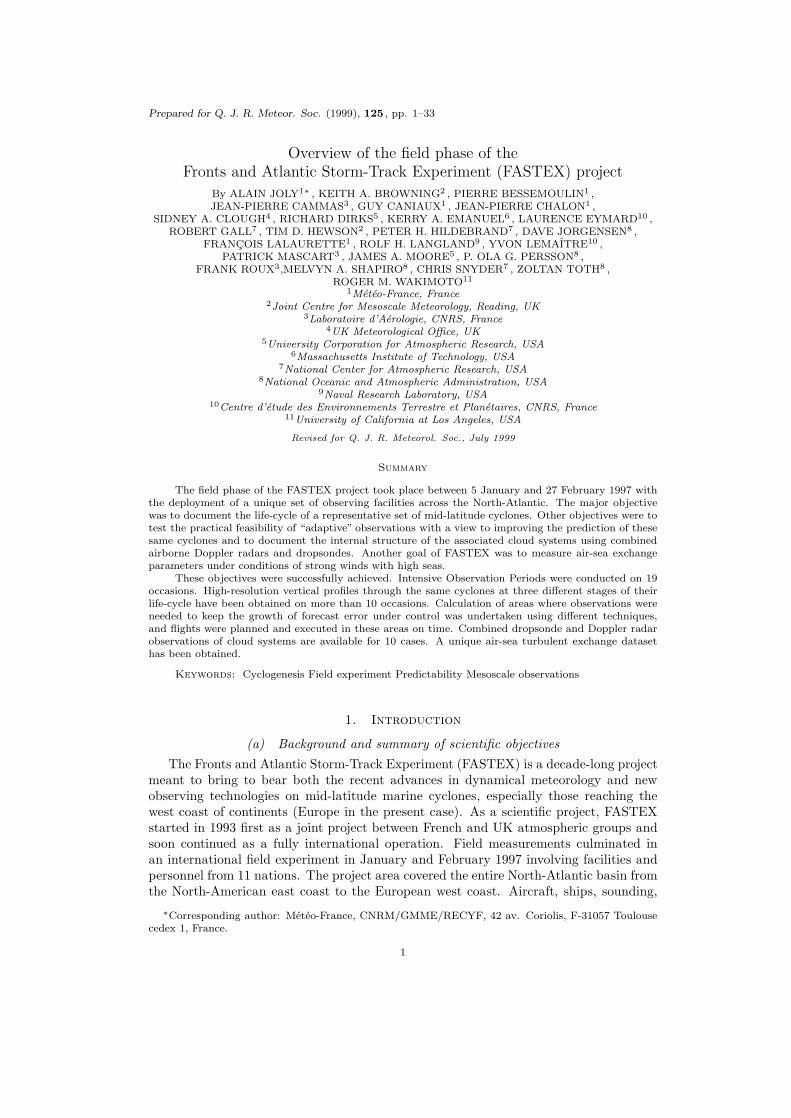
Figure 1. The map shows the North-Atlantic area divided into three adjacent zones where the FASTEXplatforms were deployed sequentially. The lower part of the figure shows the ideal deployment along thetrack of a single event together with an idea of the time-scale.

adaptive observing.• To document the meso- and micro-scale organization of cyclone cloud systems. On

the longer time-scales, mid-latitude storm-track cyclones are essential components ofthe climate system. They generate most deep layer clouds at these latitudes; theyalso provide much of the significant rainfall. Thus FASTEX is also meant to studycyclones in the perspective of the GEWEX∗ Cloud System Study (GCSS) (Browning,1994). There are two types of issues in this area:

– to document the internal organization of layered clouds, which is very partiallyknown at present (see Ryan 1996 and Stewart et al. 1998 for recent detailedreviews). An interesting feature is the multiple layering and the associated complexvertical distribution of latent heating and radiative feedback.

– to study the importance of the fine structure underlying the average properties ofthese rather large-scale cloud decks. Most of these “anomalies” in the organisa-tion are, in fact, mesoscale organizations taking the form of patches and bands

∗Global Energy and Water budget Experiment. Other acronyms are defined in Appendix A.

4 A. JOLY et al.

(see above references and e.g. Parsons and Hobbs, 1983). Although occupying arelatively small fraction of the whole system, they concentrate significant parts ofthe rainfall generation, stronger radiative impact through thicker or higher clouds,etc. The actual influence of these sub-structures, as well as their life-cycles andorigins remain to be determined.

The longer term goals in this area are to establish the water budget and precipitationefficiency of these cloud systems together with a better knowledge of their radiativeimpact. In practice, this knowledge will be used possibly to develop and in any case toprovide validation data for new-generation cloud parameterization schemes includingat least one explicit condensed water variable. The better knowledge of the mecha-nisms leading to mesoscale structures will also help in improving local, short-rangeforecasting.

• To measure turbulent air-sea fluxes under strong winds and high seas. Important ef-forts have been made, in the past decade, to improve the description of turbulentexchanges between the earth’s surface and the atmosphere. These processes are im-portant for both short-range forecasting (prediction of near-surface conditions) andclimate simulations. The recent field experiments have measured these fluxes overdifferent types of ground and vegetation. However, most of the earth’s surface is, infact, a sea surface and little is known about turbulence in the middle of ocean basinsduring high wind speeds. There are very few or no observations available for windsstronger than 15 ms−1. Thus FASTEX was also planned to obtain measurements inthis particular parameter domain. The aim is to improve the parameterizations of tur-bulent fluxes as well as to be in a position to analyse the influence of these exchangeson the cyclone properties. Air-sea fluxes measurements were also the meteorologicalcomponent of the Labrador Sea Deep Ocean Convection Experiment that took placeat the same time as FASTEX (Marshall et al., 1998).

(b) Objectives of the field phaseEssential components of these objectives are difficult to address with existing datasets.

The key to FASTEX as a field project is contained in the idea that the evolution of cy-lones is likely to be more complex than the continuous growth of some kind of instabilityfollowed by a non-linear saturation process. This statement immediately leads to therequirement that entire life-cycles have to be documented. Important (and not so recent)ideas on cyclogenesis involve the existence of precursor systems and the possibility oftransient interactions between such systems or other flow organizations such as fronts.In order to check these ideas on real cases as directly as possible, cyclones have to betracked across the ocean throughout their life-history.

It follows that the primary experimental objective of the field phase of FASTEX isto perform numerous direct observations of the structure of the same cyclones at severalkey stages of their life-cycle. The data should, ideally, take the form of precise verticalprofiles of the key dynamical quantities (wind, temperature, humidity) covering the wholedepth of the troposphere and the lower stratosphere.

Another goal of the field phase is to perform the first real-time implementation ofan adaptive observing system for reducing forecast errors for selected cyclones. Thisrequirement is a priori quite independent from the one of adapting the observing systemin order to capture the growth of an actual cyclone. Since forecast-error control involvesthe use of well defined numerical algorithms in order to determine the key areas, theFASTEX scientists tended to call this component of FASTEX “objective targeting”. The

OVERVIEW OF THE FIELD PHASE OF FASTEX 5

TABLE 1. Major facilities and participating institutionsinstruments, owner, crew’s Funding

Facility functions home institution agencyCC ÆGIR radiosoundings (GPS) Icelandic Coast Guard EC

(IS)RV KNORR radiosoundings, (Ú) Woods Hole NOAA

profilers, fluxes (USA)RV LE SUROÎT radiosoundings, (GPS) IFREMER CNRS, EC

profilers, fluxes (F)RV V. BUGAEV radiosoundings (GPS) UkrSCES Météo-France

(Ukraine)C-130 (UK) dropsoundings (GPS) UK Met Office UK Met OfficeC-130 (USA) dropsoundings (Ú) US Air Force US Air ForceELECTRA Doppler radar NCAR (USA) CNRS, NSFGULFSTREAM- dropsoundings (GPS) NOAA (USA) NOAA, Météo-France,IV CNRS, NRLLEARJET dropsoundings (GPS) FIC (USA) NSFWP-3D (P3) radars (1 Doppler), NOAA(USA) NOAA, CNRS,

dropsoundings (GPS) Météo-FranceIncreased soundings 6h soundings CAN, Greenland, Countries,on a regular basis IS, IE, UK, F, SP, WMO,

Azores (P), ECBermuda, DK

Increased soundings 6h soundings USA NCAR, NOAAon alert 3h soundings IE, F, UK Countries

Buoys surface obs. EGOS EGOSOperations Centre monitoring, Aer Rianta ECat Shannon forecast (IE)Staff of Shannon forecasters, CNRS(F), CMC(CAN), Institutions,Ops Centre and scientists JCMM(UK), NSF,Scientific crews Met Eireann(IE), EC

Météo-France(F),NCAR(USA),NOAA(USA),NRL(USA),

UCAR(USA),UCLA(USA),

UK Met Office(UK)Staff of US forecasters, MIT(USA), NOAA,targeting operations scientists NCEP(USA), NSF

NCAR(USA),Penn State U.(USA),U. of Wisconsin(USA)

Agencies without direct participation: European Commission (EC),European Group on Ocean Station (EGOS),National Science Foundation (USA),World Meteorological Organisation (WMO).

GPS: wind measurement technique based on the satellite Ground Positioning System.Ú: wind measurement technique based on the Omega navigation system.see Appendix A for other acronyms.Selected Country Codes: CAN: Canada, DK: Denmark, F: France, IE: Ireland,

IS: Iceland, P: Portugal, SP:Spain.For details on instruments and platforms, see either Joly et al. (1997)or the FASTEX Data Base online documentation (section 8).

6 A. JOLY et al.

task of observing different stages in the cyclone life-cycle, on the other hand, depends onreading synoptic charts and looking at satellite images with concepts in mind, and in thiscase the method of selecting critical features was commonly referred to as “subjectivetargeting”.

The primary objective concerning the organisation of mature cyclones was to describetheir three-dimensional precipitation and wind structure over a 1000 by 1000 km domainusing a combination of dropsondes and airborne Doppler radar. These sensors weredeployed in a manner that systematically covered as much of the cyclone with a regulargrid of data assimilation and validation of numerical simulations.

Finally, another objective deriving directly from the scientific objectives mentionedpreviously is to document turbulent fluxes in high winds in mid-ocean. The article byEymard et al. (1999) provides the details and some results.

The present overview is meant to give a first idea of how well these goals havebeen reached. It is laid out as follows. The next section summarizes the plans foroperations and the facilities available and section 3 summarizes the large-scale weathercharacteristics during FASTEX. Then, two examples of FASTEX cases are presented soas to convey an impression of the type of systems of interest and of the type of operations.These sections are meant for readers who are looking for story-like accounts of whatFASTEX operations really are. Those readers only looking for overall information mayskip these sections and go directly to a summary of all operations and a preliminarysubjective characterization of all the cases which is presented in section 6. Two shortsections address the forecasts (section 7) and the Data Base (section 8). The articleconcludes with comments on the outcome of the operations (section 9).

2. Observing strategy and platforms

In order to achieve the primary experimental objective of FASTEX, namely to fol-low a number of cyclones throughout their life-cycle, a special distribution of observingfacilities had to be devised (Fig. 1). The North-Atlantic area has been divided intothree adjacent areas: the “Far Upstream Area”, centered on the airport of St John’s inNewfoundland, the mid-stream area, centered about the longitute 35oW and the Multi-scale Sampling Area (often termed MSA). The Multiscale Sampling Area was focusedon Shannon airport in Ireland.

The purpose of enhancing observations in the Far Upstream Area is to observe theearly stages of the formation of a new cyclone, possibly its genesis. The Far UpstreamArea is also the primary area for collecting the observations for the predictability (tar-geting) objectives.

The purpose of enhancing observations in the midstream area is to fill, as well aspossible, the well known “data void” in the middle of the oceanic basin. It is located atthe end of the most persistent (or least variable) part of the storm-track, a very goodplace to catch the developing phase of many cyclones. It is also a good location forfrequent encounts of the strong winds and high seas required for the measurements ofair-sea fluxes.

Finally, the Multiscale Sampling Area is where the mature cyclones and their cloudsystem are to be observed with, as the name suggests, the possibility to collect data ontheir structure at several different scales.

Table 1 summarizes the observing platforms and instruments available for FASTEX.It also provides the list of institutes, agencies and organizations that have supported theproject. A much more detailed table on instruments and facilities can be found in Joly

OVERVIEW OF THE FIELD PHASE OF FASTEX 7

~ 27 JAN -6 FEV

~ 6 JAN -26 JAN

~ 7 FEV -27 FEV 97

Figure 2. A summary in 3 sketches of the ac-tual observing platforms that were deployedduring the field phase of FASTEX, also show-ing the location of the upper-air stations in-volved. The shaded zones refer to the areas ofFig. 1. The dates are somewhat approximate,since, for example, the ships were still operat-ing en route when calling to ports in the middleperiod. The graphic symbols for ships, turbo-prop and jet aircraft can readily be identifiedto the facilities listed in Table 2.

et al. (1997). The present table has been updated with the actual facilities available,but there are few changes.

The bottom half of Fig. 1 shows the basic strategy to deploy these facilities in thecourse of a FASTEX Intensive Observations Period (IOP), namely successively in time,for a period that can be as long as 60 h. A further lead time of 30h to 42h is needed forlogistical reasons. The “constitutive” decision to launch an IOP has to be taken, therefore,on the basis of 84h or 96h forecast products. It depends on the strong expectation ofa significant cyclone moving into the Multiscale Sampling Area: the estimated timefor this to happen sets the reference date, denoted 0h in Fig. 1. This decision-takingproblem can by called the “FASTEX dilemma”: FASTEX is motivated by the difficultyof making reliable cyclogenesis forecasts at practically any range but for FASTEX tocollect the data required to understand this problem, reliable medium-range forecasts arerequired. One practical step that was taken was to transmit in real time via the GlobalTelecommunication System as many extra observations as possible so as to improve theperformance of the operational numerical weather prediction systems.

The diagram in Fig. 1 also shows the main facilities and the way they were em-ployed in FASTEX. It does not show the significant uplift of the background observationnetwork made from the conventional World Weather Watch upper-air stations: fromCanada to Bermuda, including Greenland, Iceland, the Faroes, Ireland, the Azores andthe European west coast, about 30 stations performed 6-hourly soundings during thewhole two months of the FASTEX field phase. A number of commercial ships equippedfor launching sondes more or less automatically also contributed to this improvement.The USA similarly re-inforced 4 of their stations but on an alert basis. Furthermore, thenumber of drifting buoys in the Central Atlantic has also been significantly increased.In these ways, practically all cyclogenesis events that took place within the two monthsare better documented than usual.

The main aircraft employed during FASTEX are a LearJet based in St-John’s andoperating in the Far Upstream Area, temporarily reinforced by two C130s from theUS Air Force. The Multiscale Sampling Area was covered by the C-130 from UKMO,

8 A. JOLY et al.

the Electra from NCAR and one P3 from NOAA. All areas could be reached by theGulfstream IV jet of NOAA, normally based in Shannon, but located in St-John’s onoccasions. Finally, the backbone of the midtsream observations is a set of up to fourships.

Early in the planning of FASTEX, it was realised that the ships, in order to beuseful all the time, would have to remain in the vicinity of the main baroclinic zone.The effectiveness of this approach was demonstrated in an idealized observing systemsimulation experiment (Fischer et al., 1998). The idea of having ships moving with aweather feature in the middle of the ocean generated many comments from reviewersof the project. The idea, however, was simply to compensate for the relatively slowmeridional motions resulting from the low frequency evolution of the flow, not to trackthe cyclone themselves. Practical experience during FASTEX revealed that this ideawas quite feasible: the predictability on this scale was good enough and the resultingdisplacements manageable in spite of difficult seas.

A climatological study partly summarized by Ayrault et al. (1995) suggests that,in order to be able to sample ten cyclones well, a period of two months is needed.FASTEX was planned on that basis. The detailed plans of operations, together with thevarious flight patterns to be considered for the different types of aircraft and missions,are described in the FASTEX Operations Plans (Jorgensen et al., 1996). The actualobserving system available during the two months field season is shown in Fig. 2. Roughlyspeaking, the observing problems divided into three periods. During the first period theGulfstream aircraft was largely unavailable. During the second period, the ships hadto call into ports. During the last period the Electra aircraft had to be withdrawn formechanical reasons. One of the ships (the RV Knorr) was reassigned to another project,the Labrador Sea Deep Convection Experiment (Marshall et al., 1998). However, thecrew still maintained a link with FASTEX and actually took part in some IOPs. On thepositive side, the first period was run with four ships as planned and an intercomparisonof the flux measurements took place; all the other components performed quite well. Inparticular, the first complex coordinated flights in the Multiscale Sampling Area were asuccess. In the second period, the Gulfstream became fully available and two C-130 wereprovided by the US-Air Force: they took part mostly to the test of adaptive observationsbut, to some extent, they also replaced the ships (as in IOP 9, for example). Finally,during the last period, when some of the most interesting cyclones occurred, all theavailable components were employed at their full potential.

3. Meteorological conditions

The notion of weather regime, as defined by Vautard et al. (1988), is useful forhighlighting conditions favourable to the type of event of interest to FASTEX. A regime,in this sense, is a quasi-steady configuration of the large-scale flow. The regimes, listedin order of increasing suitability for FASTEX, are known as the Blocking regime, theGreenland Anticyclone (or Southern Zonal) regime and the Zonal regime.

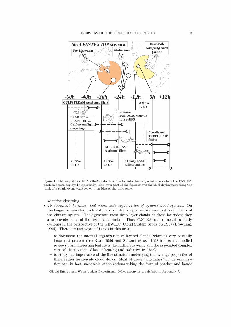
Averaged meteorological conditions relevant to the FASTEX period are displayed inFig. 3. Analysed fields have been projected on the weather regime fields to determine,daily, the closest one. On this basis, it appears that there are three distinct periods. Theyear 1997 starts with a fortnight of Greenland Anticylone regime, although in practice, itis more an Icelandic ridge than a true anticyclone. The actual mean flow for this period,although close to this reference climatological regime, also shares some characteristics ofthe highly unfavourable Blocking Regime. Thus systems remain at relatively southernlatitudes in general but are able, on occasion, to move north-eastwards and to establish

OVERVIEW OF THE FIELD PHASE OF FASTEX 9

288

278

298

288

278

258

268

298

(a) mean flow from 1 JAN to 13 JAN

(b) mean flow from 14 JAN to 2 FEB

(c) mean flow from 3 FEB to 28 FEB

Figure 3. A summary of the averaged meteorological conditions during FASTEX. Contours are 700 mbargeopotential (every 5 damgp) and the three intensities of shading indicate 300 mbar wind in excess of40, 45 and 50 ms−1. Figure prepared by B. Pouponneau, Météo-France, using the ARPEGE analysesincluded in the Data Base.

10 A. JOLY et al.

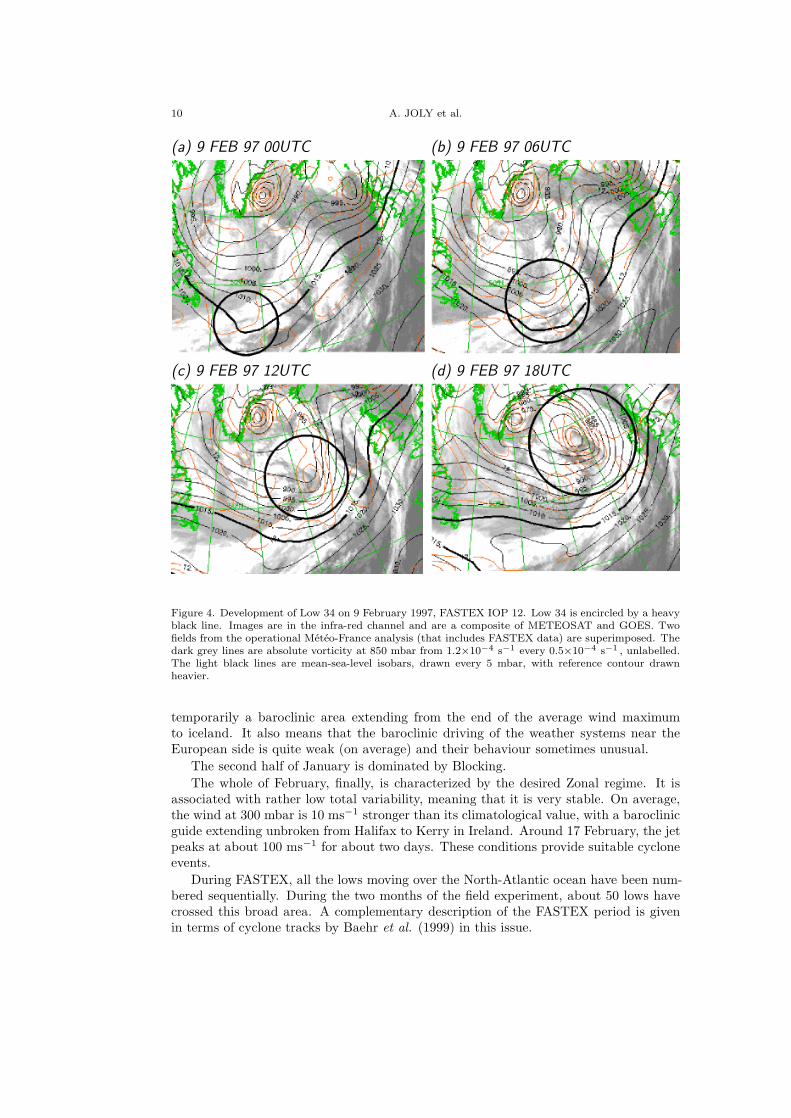
(a) 9 FEB 97 00UTC (b) 9 FEB 97 06UTC

(c) 9 FEB 97 12UTC (d) 9 FEB 97 18UTC

Figure 4. Development of Low 34 on 9 February 1997, FASTEX IOP 12. Low 34 is encircled by a heavyblack line. Images are in the infra-red channel and are a composite of METEOSAT and GOES. Twofields from the operational Météo-France analysis (that includes FASTEX data) are superimposed. Thedark grey lines are absolute vorticity at 850 mbar from 1.2×10−4 s−1 every 0.5×10−4 s−1 , unlabelled.The light black lines are mean-sea-level isobars, drawn every 5 mbar, with reference contour drawnheavier.

temporarily a baroclinic area extending from the end of the average wind maximumto iceland. It also means that the baroclinic driving of the weather systems near theEuropean side is quite weak (on average) and their behaviour sometimes unusual.

The second half of January is dominated by Blocking.The whole of February, finally, is characterized by the desired Zonal regime. It is

associated with rather low total variability, meaning that it is very stable. On average,the wind at 300 mbar is 10 ms−1 stronger than its climatological value, with a baroclinicguide extending unbroken from Halifax to Kerry in Ireland. Around 17 February, the jetpeaks at about 100 ms−1 for about two days. These conditions provide suitable cycloneevents.

During FASTEX, all the lows moving over the North-Atlantic ocean have been num-bered sequentially. During the two months of the field experiment, about 50 lows havecrossed this broad area. A complementary description of the FASTEX period is givenin terms of cyclone tracks by Baehr et al. (1999) in this issue.

OVERVIEW OF THE FIELD PHASE OF FASTEX 11

K

Æ

B

S

IOP 12Low Track; 9 FEB 06 UT

Low levelprecursor8 FEB

US C1309 FEB 13UT Gulfstream

8 FEB 14UT

US C1308 FEB 06UT

P3, C1309 FEB 18UT

Figure 5. Schematic diagram of the operations during IOP 12. The large dots form the track of Low 34,marked every 6h, an open circle corresponding to an open wave. The dotted area indicates the zonewhere the surface precursor formed. The ships are shown at their location during the phase of intensivesoundings. All upper-air stations shown (balloon symbols) were operating every 6h except the darkestones which were operating every 3h. The tracks show the various successful flights. The difficult andeventful St-John’s–Shannon flight of the Gulfstream IV on 9 Feb is not shown because no data weretaken.

4. Example of an Intensive Observations Period: IOP 12

The best way to convey a flavour of FASTEX operations is to summarize the story ofone Intensive Observing Period. Readers familiar with field operations spanning severaldays from one side of an ocean to the other may jump to the general overview in section 6.Because of its unique mixture of exciting meteorology and dramatic operational events,IOP number 12 is now presented.

The meteorology is discussed first. IOP 12 is conducted on Low 34. This cycloneundergoes, on 9 February 1997, the most explosive deepening of the period: roughly−54 mbar in 24h, with a phase of −23 mbar in 6h. This very rapid development goesalong with a very short life-cycle. It is summarized by Fig. 4. The background showsinfra-red images composited from both geostationary satellites GOES and METEOSAT.The figure also shows the mean-sea-level pressure and low-level vorticity analyzed bythe Météo-France operational suite ARPEGE. An individual vorticity maximum can betracked from 9 February 00UTC onwards, whereas closed isobars can be seen only whenthe low is fully developed, after 18UTC. The analysed sea-level pressure falls from about1015 mbar on 8 February 18UTC to 961 mbar on 9 February 18UTC. Between 6UTC and18UTC 9 February, Low 34 moves about 1700 km at a phase speed of nearly 40 ms−1.

The first tentative plan for a possible IOP 12 on a Low 34 is drafted on the basis ofthe forecasts starting on 5 February 00UTC and, for the ECMWF model, 4 February12UTC. As the Low is expected to be in the western part of the MSA on 10 February00UTC, it is important to note that these are 120h and 132h respectively. As summarizedin section 7 below, decisions for FASTEX are prepared using an “ensemble” of manydifferent numerical models. Needless to say that there is a wide discrepancy in the

12 A. JOLY et al.

various forecasts, but at the same time, there is enough consistency to convince theteam of forecasters that a new IOP may be declared. As soon as 5 February 12UTC,a westbound flight of the Gulfstream-IV jet aircraft is planned for 8 February, a returnflight on 9 February and a coordinated MSA flight of turboprop aircraft on 10 February.The case is believed, at that time, to be a rapid deepener.

These decisions are confirmed on the following day, that is 2 days prior to the firstairborne operation relating to IOP 12, and 3.5 days before the cyclone speeds into theMSA. The ships are informed of the likely IOP scenario and that they will have to perform3h radiosoundings for 24 hours as from 8 February 12UTC. On 6 and 7 February, theday prior to the beginning of IOP 12, the discrepancy between the various forecastsbecomes quite large and Low 34 turns into an unexceptional event except in the 72hARPEGE forecast. These are signs that the case is a good one for testing the adaptiveobservation strategy: specific targets for this system are determined by the variousgroups involved in this aspect of FASTEX: the NRL in Monterey, NCEP in Washington,ECMWF in Reading and Météo-France in Toulouse. Contacts are made between theproject headquarters at Shannon and Washington to try to coordinate “targeting” flightsbetween aircraft already based in St-John’s and the Gulfstream-IV, set to join themon 8 February. A few more soundings are ordered from the ships in order to face newpossibilities, including another wave cyclone.

The actual operations managed on this case are summarized by Fig. 5. Low 34behaves more or less as anticipated from the 48h or so forecast runs. The Gulfstream-IVproperly samples the predictability “target”. The ships, although fully in the track of thecyclone and accompanying gale force winds, manage to perform the required soundings.The USAF C-130 flight on 9 February samples the wake of Low 34 in case a secondaryLow 34B shows up (the data may help explain why it did not). However, shortly afterthe Gulfstream-IV took off from St John’s for what should be an optimal flight samplingthe structure of a deepening cyclone, one of its electric generators stops functioning.The flight is completed safely, albeit with much anxiety. Then, there is the possibility tostudy the detailed structure of the cloud system with dropsondes from the C-130 and bothairborne Doppler radars. The UKMO C-130 and the P3 aircraft take off successfully butthe mechanical problem of the Electra prevents it to join them. Radio communicationswith the other two turboprops allows for in-flight adjustment of the plans to compensatefor the absence of the Electra and a successful operation results. Valuable data has beenobtained at various stages of the evolution of Low 34 .

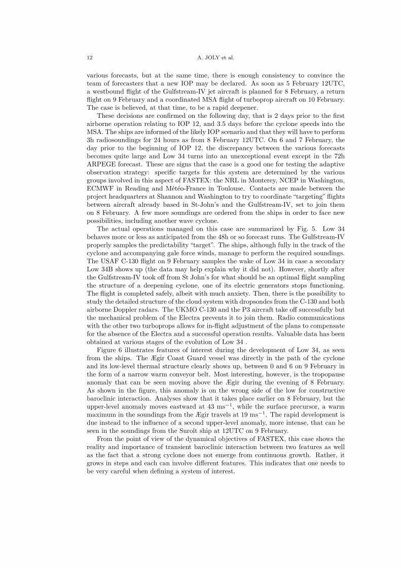
Figure 6 illustrates features of interest during the development of Low 34, as seenfrom the ships. The Ægir Coast Guard vessel was directly in the path of the cycloneand its low-level thermal structure clearly shows up, between 0 and 6 on 9 February inthe form of a narrow warm conveyor belt. Most interesting, however, is the tropopauseanomaly that can be seen moving above the Ægir during the evening of 8 February.As shown in the figure, this anomaly is on the wrong side of the low for constructivebaroclinic interaction. Analyses show that it takes place earlier on 8 February, but theupper-level anomaly moves eastward at 43 ms−1, while the surface precursor, a warmmaximum in the soundings from the Ægir travels at 19 ms−1. The rapid development isdue instead to the influence of a second upper-level anomaly, more intense, that can beseen in the soundings from the Suroît ship at 12UTC on 9 February.

From the point of view of the dynamical objectives of FASTEX, this case shows thereality and importance of transient baroclinic interaction between two features as wellas the fact that a strong cyclone does not emerge from continuous growth. Rather, itgrows in steps and each can involve different features. This indicates that one needs tobe very careful when defining a system of interest.

OVERVIEW OF THE FIELD PHASE OF FASTEX 13

24.

32.

40.

48.64.

24.

16.

8.

60.

20.

40.

40.

40.

60.

SUROÎTMean position:34.0°W,48.5°N.

8 FEB 97 00UTto

10 FEB 97 00UT

1000.0. 0.12. 12.18.18.0.

9 FEB 8 FEB6. 6.

900.

800.

700.

600.

500.

400.

300.

200.

24.

32.40.

48.

48.

64.

24.16

.

ÆGIRMean position:34.5°W,45.5°N.

8 FEB 97 12UTto

10 FEB 97 00UT

1000.0.12. 12.18.18.0.

9 FEB 8 FEB6.

900.

800.

700.

600.

500.

400.

300.

200.

60.

60.

75.

40.

20.

20.

40.

Figure 6. Vertical-time cross-sections derived from the radiosoundings taken from RV Suroît (left) andCC Ægir (right) during IOP 12. The time scale has been reversed so that the figures are suggestive ofvertical cross-sections with West to the left and East to the right. The heavy solid lines show the windspeed every 5 ms−1. The light solid lines are θw every 2 K. Light grey shading marks the location ofvery dry air (less than 40 % relative humidity). Darker shading indicates likely cloudy areas (more than80 % relative humidity). The small crosses indicate the data points. The analysis has been performedwith spline functions. Figure derived from the soundings from the FASTEX Data Base, courtesy ofG. Desroziers from Météo-France for the analysis.

5. The Lesser Observations Periods during FASTEX

According to the previous section critical decisions regarding IOP 12 are taken 3 daysbefore the system even existed. Difficulties raised by the differences between forecastshave been alluded to, and there are others resulting from operational constraints. Itis because of the operational constraints that Low 33 (top right corner of Fig. 4(a)),although the type of system of interest to FASTEX, was not the subject of intensiveobservations: the rapid succession of IOPs 9 to 11 imposed a break in the operations.

Yet Low 33 is by no means totally deprived of special observations. 54h prior toLow 33 entering the MSA, a long flight of an USAF C-130 from St-John’s covered the

14 A. JOLY et al.

288.

304.

320.

0.

0.

20.

20.

40.

1000.

900.

0. 500. 800. km

800.

700.

600.

500.

400.

300.

22 FEB 9720UT to 21UT 53°N, from 24°W to 12°W

Figure 7. Vertical cross-section derivedfrom the dropsoundings taken from theGulfstream-IV aircraft at the end of aflight part of IOP 18, but describingthe cyclone 42B that was not selectedfor an IOP. Contours and shading areas in Fig. 6 , except θw drawn every4 K. The analysis has been performedwith spline functions by G. Desroziersusing the FASTEX Data Base.

broad area around 50oW and 45oN where the low starts to form later. The ships are onthe track of this low as well and performed 8 soundings per day on 7 and 8 February asLow 33 developed. And finally, as the Gulfstream flies towards St-John’s on 8 February,it samples the same low, still undergoing deepening, with a series of dropsoundings,providing a minimum set of data in the MSA. These are the components of a mildlysuccessful IOP and so this case has been included in the FASTEX set. It was, indeed,labelled IOP 11A for a time.

Low 33 is not an isolated case. After the field phase was completed, a second setof systems has been added to the main FASTEX Intensive Observations Periods: theFASTEX Lesser Observations Periods (FLOP). They fall into two categories: the firstis made up of the cases like Low 33 that are only partially covered for logistical reasons.The second category is, given the objectives of the project, quite an important one: itcontains the cases only partially covered because they are wrongly anticipated by theforecasts. They epitomise the “FASTEX dilemma” mentioned in section 2 Since FAS-TEX is about understanding predictability, looking back on these cases can be helpful.Figure 7 illustrate a case falling in the second category, one model only having predictedits existence at the time a decision had to be made for an IOP 18. This figure also showsthe capabilities of the Gulfstream-IV to map cyclone-scale features. These two cases arenow included in this series of interesting cases as LOP 2 and LOP 5.

6. Summary of operations and overview of cases

This section takes a broader perspective and presents the complete set of FASTEXcases. There are 25 of them: 19 IOPs were declared and run as such, 6 LOPs wereincluded at the end of the field phase, when the whole period was reassessed (FASTEXwas initially planned to allow the study of 10 cases). Almost all cases concentrate on aparticular type of cyclone or on a feature such as a front that did not allow for a cyclone

OVERVIEW OF THE FIELD PHASE OF FASTEX 15

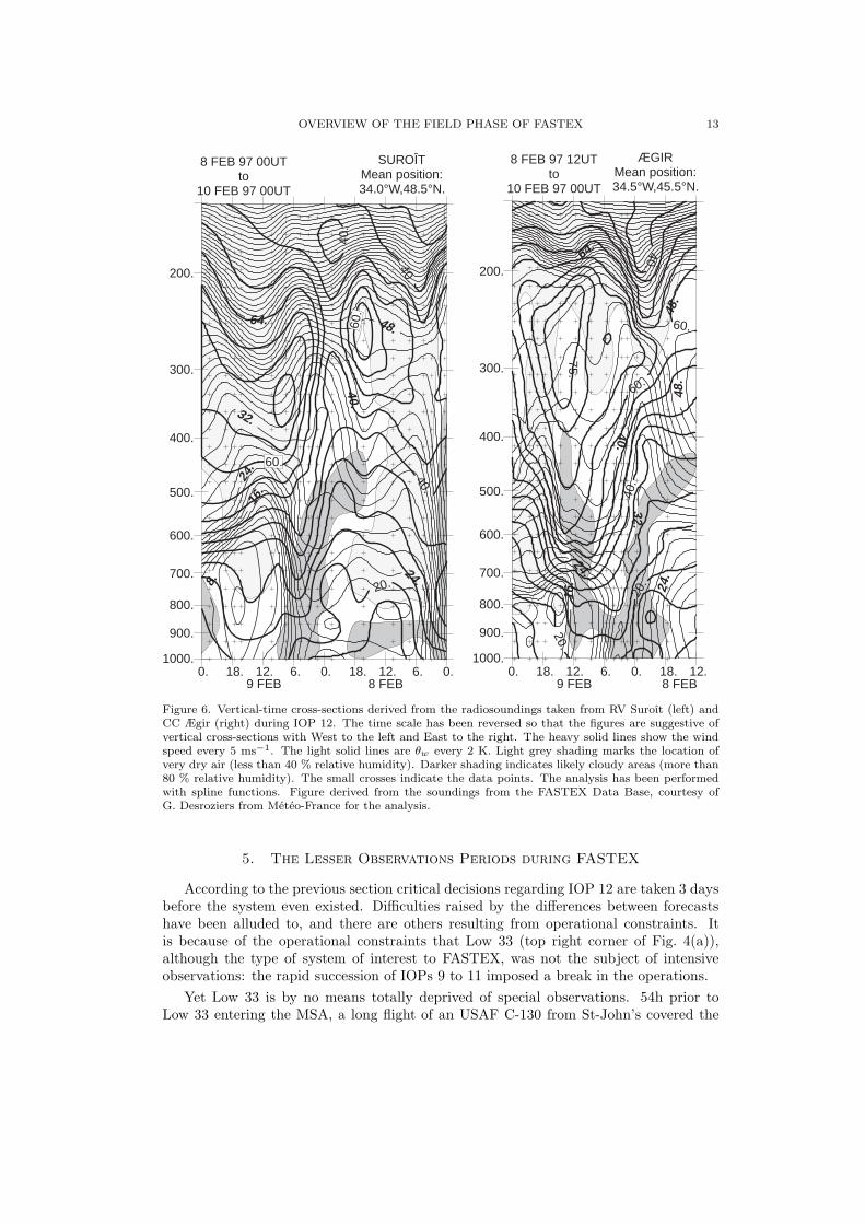
TABLE 2. Summary of operations on each FASTEX caseSoundings Upstream Ship Upstream Ship MSA Airborne 3hourly

at 3 data data data data sampled Doppler Europeansuccessive for for for for with data in west-coast

stages targeting targeting dynamics dynamics dropsondes MSA soundingsIOP 1 – – – – end ampli • ss ∗∗ ∗∗LOP 1 – – 24h – beg ampli – – ∗∗IOP 2 • 36h 48h – – • mi ∗ ∗ ∗ ∗∗IOP 3 – 48h 24h gen ampli – – ∗∗IOP 4 – – 48h – organ – – ∗∗IOP 5 • 48h 36h – organ • mi ∗∗ ∗∗IOP 6 – – 18h – beg sup • – ∗∗IOP 7 – – 18h – front • • ss ∗ ∗ ∗ ∗∗IOP 9 • 42h (C130) ampli (circl) • mi ∗∗ ∗ ∗ ∗IOP 10 • 18h 30h gen beg gen • ss ∗ ∗ ∗ ∗ ∗ ∗IOP 11 • 36h 18h beg ampli front • • ss ∗∗ ∗∗LOP 2 • 48h 18h – ampli • – –IOP 12 • 30h 12h rear gen beg ampli • ss ∗∗ ∗ ∗ ∗IOP 13 – 48h 48h circl beg dec – – –LOP 3 – 48h 48h – beg gen – – –IOP 14 – 48h 24h – beg dec – – –IOP 15 • 24h 18h rear ampli • ss ∗∗ ∗IOP 16 • 24h 12h – beg gen • ss ∗ ∗ ∗ ∗ ∗ ∗LOP 4 – 48h 24h – clust – – ∗ ∗ ∗IOP 17 • 42h 18h ampli 1 wave • • ss ∗ ∗ ∗ ∗ ∗ ∗LOP 5 – – 36h – beg gen • – –IOP 18 • 36h 12h gen ampli • mi ∗∗ ∗ ∗ ∗LOP 6 – 48h 36h – beg dec – – ∗ ∗ ∗IOP 19 • 30h 24h wave sup waves • – ∗∗Abbreviations for life-cycle stages: beg: early step of stage

gen: genesisrear: rear (western) componentcircl: soundings all around systemclust: cloud cluster

ampli: amplification, deepening stage(s)organ: organisation, "shaping"

sup: suppression (of waves)dec: decay.

Symbol • means "yes" or "present"Symbol • • marks that 2 sets are available.Targeting lead times: the figures are orders of magnitude based on the life-cycle of thesystems. They are not the exact values employed by a particular targeting group.Coverage in the MSA: ss: systematic survey

mi: mesoscale investigation∗∗: 70–80% sucess rate of sampling

∗ ∗ ∗: 100% success rate of sampling.From IOP 12 onwards, the Electra is removed.European west-coast radiosoundings:∗ means that only the UK stations actually on the west coast were active.∗∗ means that only the stations actually on the west coast were active.∗ ∗ ∗ means that all the participating stations were active.

to form. All these cases are in line with the objectives of the project: the sole exceptionis IOP 8. IOP 8 takes place, during the blocking period, when no cyclone can possiblyreach the eastern Atlantic. In order to maintain a minimum of activity, a flight from theGulfstream is set up and directed towards Greenland in order to document upper-levellee waves. However, apart from the fact that the flight intersects a coastal front, thisIOP is difficult to include in the summary tables fitted for cyclones.

The achievements of the field phase of FASTEX are summarized in Table 2. Ap-

16 A. JOLY et al.

40ON

50ON

60ON

0OW

70OW 60OW 50OW 40OW

: G IV (17/02 15Z-20Z) : dropsondages

18Z

D957

975

975

80

980

985

985

9

990

995

995

1000

1005

1010

1015

1020

1050ON

55ON

60ON5OW

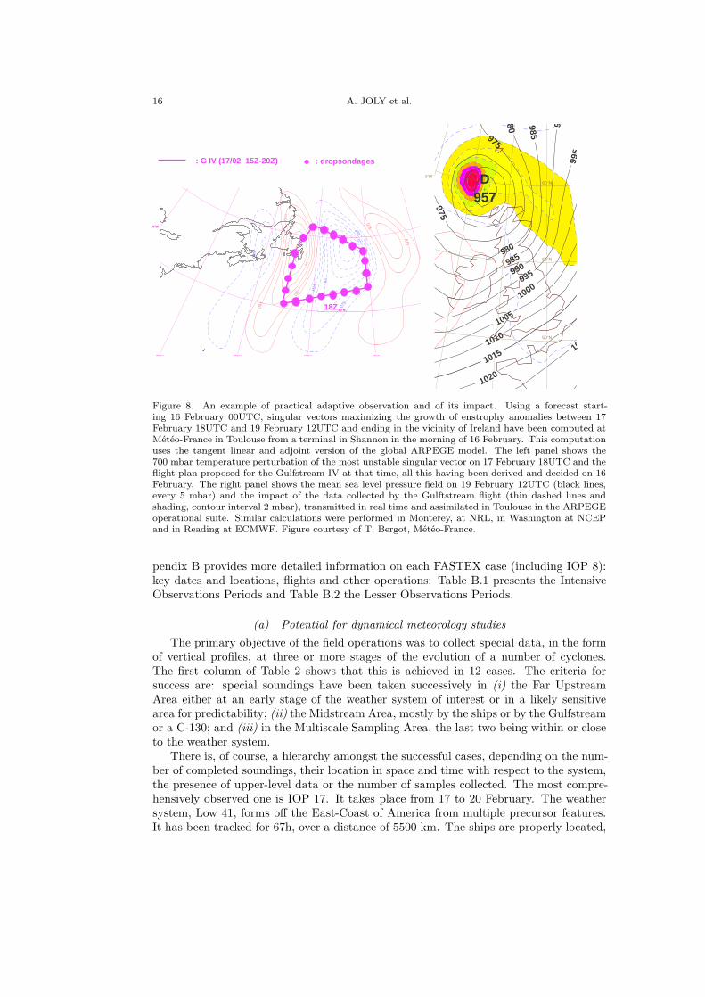
Figure 8. An example of practical adaptive observation and of its impact. Using a forecast start-ing 16 February 00UTC, singular vectors maximizing the growth of enstrophy anomalies between 17February 18UTC and 19 February 12UTC and ending in the vicinity of Ireland have been computed atMétéo-France in Toulouse from a terminal in Shannon in the morning of 16 February. This computationuses the tangent linear and adjoint version of the global ARPEGE model. The left panel shows the700 mbar temperature perturbation of the most unstable singular vector on 17 February 18UTC and theflight plan proposed for the Gulfstream IV at that time, all this having been derived and decided on 16February. The right panel shows the mean sea level pressure field on 19 February 12UTC (black lines,every 5 mbar) and the impact of the data collected by the Gulftstream flight (thin dashed lines andshading, contour interval 2 mbar), transmitted in real time and assimilated in Toulouse in the ARPEGEoperational suite. Similar calculations were performed in Monterey, at NRL, in Washington at NCEPand in Reading at ECMWF. Figure courtesy of T. Bergot, Météo-France.

pendix B provides more detailed information on each FASTEX case (including IOP 8):key dates and locations, flights and other operations: Table B.1 presents the IntensiveObservations Periods and Table B.2 the Lesser Observations Periods.

(a) Potential for dynamical meteorology studiesThe primary objective of the field operations was to collect special data, in the form

of vertical profiles, at three or more stages of the evolution of a number of cyclones.The first column of Table 2 shows that this is achieved in 12 cases. The criteria forsuccess are: special soundings have been taken successively in (i) the Far UpstreamArea either at an early stage of the weather system of interest or in a likely sensitivearea for predictability; (ii) the Midstream Area, mostly by the ships or by the Gulfstreamor a C-130; and (iii) in the Multiscale Sampling Area, the last two being within or closeto the weather system.

There is, of course, a hierarchy amongst the successful cases, depending on the num-ber of completed soundings, their location in space and time with respect to the system,the presence of upper-level data or the number of samples collected. The most compre-hensively observed one is IOP 17. It takes place from 17 to 20 February. The weathersystem, Low 41, forms off the East-Coast of America from multiple precursor features.It has been tracked for 67h, over a distance of 5500 km. The ships are properly located,

OVERVIEW OF THE FIELD PHASE OF FASTEX 17

the Suroît having moved in time to be on the track of this low. They manage, in spiteof the wind and the sea, to perform soundings every 90 minutes as the low moved overthem. Five successive flights are performed and another earlier flight, on the 16th, canperhaps also be included, from the predictability point of view. During three of theseflights, dropsondes are launched from above the tropopause. About 400 soundings aretaken in and around Low 41, 230 of which are made from the ships and the aircraft.Dynamically, this low illustrates many of the features or behaviour that led to FASTEX:non-spontaneous genesis in a complex environment, multiple phases of growth, tempo-rary tendency to split into two lows with forecast development of these centres varyinggreatly between models and explosive deepening. Some of these features are discussedin Arbogast and Joly (1998) and in the IOP 17 trilogy of Cammas et al. (1999), Malletet al. (1999a, 1999b).

It can be said, therefore, that the key experimental objective of FASTEX has beenreached. There are, furthermore, significant data for addressing more focused dynamicalissues. There are a number of rapidly developing cyclones (see Table 3 for a summary)but, as a control for checking current ideas on the way development can be hinderedunder certain circumstances, there are a few non-developing systems as well (see thework of Chaboureau and Thorpe, 1999 and Baehr et al. 1999). As will be discussedbelow, a large number of types of systems has been collected; several critical features orphases have been directly observed, such as the genesis of a wave (IOP 10), a number ofcases of the amplification phase, jet inflows and outflows. The most characteristic onesare listed in columns 4 and 5 of Table 2.

(b) Potential for adaptive observations studiesThe numerical products needed for “objective targeting” operations have been ex-

ploited in two different places: the NCEP products were analysed in Washington (USA)while the NRL, Météo-France and ECMWF products were interpreted in Shannon. Coor-dination was made possible by the presence of a representative of the Washington groupat Shannon, Dr. Snyder. See e.g. Bishop and Toth (1999), Gelaro et al. (1999), Bergotet al. (1999), Langland et al. (1999) for more details.

As a result, a large amount of data are available for impact studies on predictability.Column 2 of Table 2 lists the cases for which datasets have been obtained in the FarUpstream Area; the corresponding forecast range is also given. Note that in relativeterms the quality of short-range forecasts for some FASTEX cyclones was below that oflonger lead time forecasts. The data from the ships can be used in studies of predictabilityat the shorter ranges. They are very often well located with respect to sensitive areas.

An important aspect not reflected in this table is the experience gained in the actualpractice of “targeted observing”. The general approach is to take a 96h or 72h forecast(typically) and to calculate where data should be collected during the next 24h in orderto reduce the uncertainty at the end of the upcoming 48h forecast over a given areaor system. The earliest calculations are needed to book airspace. The next batch ofcalculations can be used to construct a flight plan. In order for the sensitive areas to beof a reasonably small size, it is necessary to focus the verification area on a particularsystem in the forecast. It has been generally possible to fly to the location determined bythe predictability calculations, but not always, because of air traffic control constraints.The actual flight time depends on a highly complicated mixture of meteorological andlogistical constraints, and so it is not practical to work with set times: all the timeparameters have to be adjusted “on the fly”. The most successful groups were thosethat considered the need for this flexibility in their planning. The feasibility of real-time

18 A. JOLY et al.

NOAA-14 VIS 1515 UTC 23 FEB 1997

P-3 Flight Track

Figure 9. NOAA-14 visible image of the cyclone of IOP 18 at 1515 UTC (left panel). Airborne Doppleranalysis of system relative winds at 2.5 km at 1540 UTC (right panel). The analysis domain of theDoppler wind field is shown by the box on the satellite image. Shading on the radar image shows thereflectivity. Figure courtesy of D. Jorgensen from NOAA.

adaptive observing has been demonstrated, but the degree of flexibility required is verysignificant. An example of target determination, associated flight plan and impact ofthe data collected as a result is shown in Fig. 8. The effectiveness of this strategy isdiscussed in the work of Szunyogh et al. (1999), Bergot (1999b), Bishop and Toth (1999),Langland et al. (1999) and Pu and Kalnay (1999).

(c) Potential for cloud-system and mesoscale studiesThis category of objective has suffered from the premature withdrawal of the Elec-

tra. Nonetheless, good datasets were collected from the very start of the field phase asindicated in the last three columns of Table 2. This is due, to a large extent, to the highdegree of cooperation achieved very early in the project by the scientists involved as wellas to their ability to explain their operations to the aircraft crews. The success is alsoattributed to the development, by the JCMM and NSSL scientists of software to per-form system-relative, multiple-aircraft flight planning. The complexity of coordinationresulted from the need subsequently to analyse the structure of the core of the cycloneswith quasi-regular flight pattern in system-relative space. In one configuration, the samesampling area is to be covered by both dropsondes and adjoining airborne Doppler radarswaths. This mode of operation, called “systematic survey” has been tested succesfullyin the very first IOP. The flight planning problem is not simple and its proper handlingby scientists and crews is one significant accomplishment of the project.

Systematic survey patterns have been achieved on 4 occasions with three aircraftand another 4 occasions with two aircraft. Bouniol et al. (1999) present results of sucha flight made during IOP 16. In four other IOPs, detailed observations of mesoscalefeatures embedded within the cyclones were obtained by airborne Doppler radars in an

OVERVIEW OF THE FIELD PHASE OF FASTEX 19

TABLE 3. Subjective synoptic characterization of the FASTEX casesClear

Comma stage Suppressedcloud- Second Rapid of waveslike generation development baroclinic (stable

feature wave stage interaction front)IOP 1 – front – • –LOP 1 – jet/front – – –IOP 2 • front – – slow genIOP 3 – – • • –IOP 4 • – – – –IOP 5 • – – – –IOP 6 – tempo – – •IOP 7 – tempo – – •IOP 9 – jet/front – • –IOP 10 – front – – –IOP 11 – – • • –LOP 2 – front – • –IOP 12 – jet/front • • • –IOP 13 – – – • –LOP 3 – front – – –IOP 14 – – – • –IOP 15 – jet/front • • –IOP 16 – jet/front • – –LOP 4 • – – – –IOP 17 – jet/front • • –LOP 5 – front • – –IOP 18 • – • • –LOP 6 – fronts – – –IOP 19 – front • • tempoSymbol • means "yes" or "present"An entry in column 2 means that the system started as a secondgeneration wave. It gives an idea of its environment, “front” beingobvious, “jet” meaning presence of a jet-streak or entrance, “tempo”meaning that waves existed temporarily or, in the case of IOP19,temporarily hindered.

environment sampled by dropsondes from the C-130. This is close to the target 10 cases.Fig. 9 illustrates the flow organisation within the cloud head of Low 44 (during IOP 18)derived from the P3 tail radar at NOAA/NSSL.

(d) Potential for air-sea interaction studiesThis component of FASTEX started as a kind of opportunistic adjunct to the project.

Its contribution to studying the complex influence of surface fluxes on cyclogenesis ad-dresses a not well resolved question. At the same time, its contribution to the problem ofparameterizing properly these fluxes in the presence of high sea and under strong windsis more clear-cut. In this area, a truly unique data set has been gathered by the Suroîtand Knorr research vessels. The required conditions have been met (indeed, the shipswere hit, on average, by a cyclone every other day) in a wide sample of vertical stabilityand temperature conditions. The reader is referred to the overview of Eymard et al.(1999) to see that this topic should soon benefit from FASTEX data.

(e) The FASTEX casesAnother important aspect is the sample of cyclone types that was covered by these

measurements. One of the ideas underlying FASTEX is that there is a large variety

20 A. JOLY et al.

of cyclones (Ayrault, 1998) and no such thing as a single type (for example, a systemgrowing on a front, always going through the same set stages and having the samestructure, as imagined earlier in this century). There is no single “typical” FASTEXcyclone. It is important that the FASTEX sample reflects this diversity.

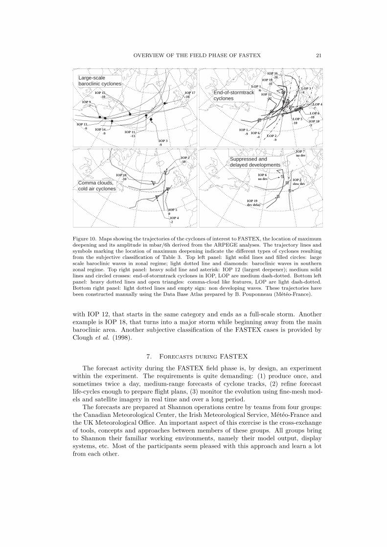
More or less in real time, B. Pouponneau, from Météo-France, prepared a basic atlasof maps based on the operational analyses made during FASTEX which included asignificant amount of special FASTEX data. These maps were soon complemented bysatellite images provided by the Data Base group (see Jaubert et al. 1999). This enablesa subjective classification of the cases to be performed based on the morphology of thesystem and its environment (Table 3).

FASTEX is primarily oriented towards cyclones forming well within the oceanicstorm-track, in contrast to East-Coast cyclogenesis as studied in programmes such asERICA (Hadlock and Kreitzberg, 1988) or CASP (Stewart, 1991). The cyclones in FAS-TEX could be called, using traditional synoptic parlance, frontal waves. However, amore general description might be second generation cyclones, suggesting they form inthe wake of another system (considered to be the parent, although this may not be alwayscorrect). This is the label retained in Table 3, and the parent structure is indicated forcyclones falling in this category of primary interest. An even better description would beend-of-stormtrack cyclones, which simply locates them geographically in a broad sense.Different views relating to the definition and description of these cyclones can be founde.g. in Kurz (1995) in relation to satellite imagery, Hewson (1997) for determining wavesautomatically or Ayrault et al. (1995) and Ayrault (1998) for composite structures ex-tracted from long series of analyses. Figure 10 shows a summary of the tracks of all themajor cyclones during FASTEX.

Table 3 shows that, apart from the non-developing and temporary small amplitudecyclones, there was a mixture of three types of systems forming well over the ocean inthe FASTEX sample: (1) cold-air cyclones dominated by convective activity and char-acterized by their comma-shaped cloud system north of the main baroclinic area (orstorm-track, roughly), (2) actual frontal cyclones and (3) cyclones forming within a com-plex environment combining a low-level front-like feature and an upper-level jet-streakor jet-entrance. A case is entered in the first column when either a comma-cloud wasinvolved in a life-cycle as precursor or the case itself was a comma cloud. The tablealso indicates the cases that developed explosively, using in a broad way the criterion ofSanders and Gyakum (1980): a phase of deepening equal to or larger than 24 mbar in24h. The presence of such a phase is shown by a dot in the “Rapid development stage”column. This happens on 9 occasions.

Table 3 identifies those systems that have a clear-cut phase of baroclinic develop-ment during their life-cycle. It means that the development of the cyclone benefits frombaroclinic interaction with an upper-level structure, typically an upper-level cyclonicanomaly: such cases are labelled as having a “clear stage of baroclinic interaction”.Cyclones having as their only feature this characteristic type of evolution (the simplestcyclones, in that sense) are not the most frequent ones: IOP 3, 11, 13, 14. Most casesadd another degree of complexity to simple baroclinic interaction, either when they aregenerated or by undergoing several phases of growth (see Baehr et al. 1999).

The last column of Table 3 lists the cases where structures such as fronts becamewavy but the waves did not develop (dot), or developed very slowly (slow gen) or sawtheir development temporarily checked (tempo).

Table 3 illustrates two levels of diversity or complexity in the FASTEX sample: theexistence of different types and the idea of complex life-cycles leading the same system tochange type. Contrast IOP 10, that remains a frontal wave throught its marine life cycle

OVERVIEW OF THE FIELD PHASE OF FASTEX 21

IOP 14-9

IOP 9-7

IOP 13-6

IOP 15-10

IOP 17-16

IOP 11-13

IOP 3-9

Large-scalebaroclinic cyclones

LOP 1-6

LOP 2-9

IOP 1-9

IOP 12-22

LOP 4-7

IOP 10-3

LOP 5-10

IOP 6-4

LOP 6-10

LOP 3-4

IOP 19-11

IOP 16-20

End-of-stormtrackcyclones

IOP 18-10

IOP 2-10

IOP 4-2

IOP 50

Comma clouds,cold air cyclones

IOP 7no dev

IOP 6no dev

IOP 19dev delay

IOP 2slow dev

Suppressed anddelayed developments

Figure 10. Maps showing the trajectories of the cyclones of interest to FASTEX, the location of maximumdeepening and its amplitude in mbar/6h derived from the ARPEGE analyses. The trajectory lines andsymbols marking the location of maximum deepening indicate the different types of cyclones resultingfrom the subjective classification of Table 3. Top left panel: light solid lines and filled circles: largescale baroclinic waves in zonal regime; light dotted line and diamonds: baroclinic waves in southernzonal regime. Top right panel: heavy solid line and asterisk: IOP 12 (largest deepener); medium solidlines and circled crosses: end-of-stormtrack cyclones in IOP, LOP are medium dash-dotted. Bottom leftpanel: heavy dotted lines and open triangles: comma-cloud like features, LOP are light dash-dotted.Bottom right panel: light dotted lines and empty sign: non developing waves. These trajectories havebeen constructed manually using the Data Base Atlas prepared by B. Pouponneau (Météo-France).

with IOP 12, that starts in the same category and ends as a full-scale storm. Anotherexample is IOP 18, that turns into a major storm while beginning away from the mainbaroclinic area. Another subjective classification of the FASTEX cases is provided byClough et al. (1998).

7. Forecasts during FASTEX

The forecast activity during the FASTEX field phase is, by design, an experimentwithin the experiment. The requirements is quite demanding: (1) produce once, andsometimes twice a day, medium-range forecasts of cyclone tracks, (2) refine forecastlife-cycles enough to prepare flight plans, (3) monitor the evolution using fine-mesh mod-els and satellite imagery in real time and over a long period.

The forecasts are prepared at Shannon operations centre by teams from four groups:the Canadian Meteorological Center, the Irish Meteorological Service, Météo-France andthe UK Meteorological Office. An important aspect of this exercise is the cross-exchangeof tools, concepts and approaches between members of these groups. All groups bringto Shannon their familiar working environments, namely their model output, displaysystems, etc. Most of the participants seem pleased with this approach and learn a lotfrom each other.

22 A. JOLY et al.

The diversity of models extends beyond the ones provided by these participatinggroups: the ECMWF model is available from several sources (for example, the IrishMet Éireann provides the 00UTC ECMWF run) and the Deutscher Wetterdienst modelis also employed on the longer ranges. On occasions, results from US models are alsoavailable.

The main outputs of the forecast teams are: (1) a medium-range forecast based onthe ECMWF ensemble, expressed in terms of weather regimes (as defined in section 3),a very good 7 day forecast of weather regime has been obtained), (2) maps of the disper-sion of cyclone centers predicted by the different models, (3) a consensus 4-day forecastof cyclone tracks resulting from comparing and discussing all the available models ex-plicitely identifying the uncertainties, for example by adding error-bars to the cyclonetracks, (4) a detailed 2-day forecast including winds and sea-state for each of the shipsand (5) detailed weather information for each of the planned flights.

8. Data collection

Sections 4 to 6 show the wide scientific potential of the measurements performedduring the FASTEX field season. An important aspect of the planning of FASTEXoperations is the early recognition of the need for easy access to data products and doc-umentation as important references for the operation planning and subsequent analysisof FASTEX cases. A FASTEX On-line Field Catalog is implemented in Shannon andmade available through the World Wide Web to all participants from all nations. Thecatalog provides ready access to project facility status, IOP and individual facility mis-sion summaries and special data products important to the field planning process. Itnow serves as a useful historical tool for analysis and other interested persons who wishto review FASTEX operations.

A critical aspect of such a project is the way these measurements are organized andmade available to the scientific community at large. From this perspective, the mostimportant legacy of FASTEX is the interactive Data Base built with these observations.The Data Base is planned early in the project. It can be accessed at the followingelectronic address: http://www.cnrm.meteo.fr/fastex/.

A large part of the Data Base has been assembled in real time: this includes all theoperational World Weather Watch data in the area of interest plus a large sample ofspecial FASTEX data, such as buoys or dropsonde profiles formatted as TEMP messages.As a result, the Data Base has been opened to general access to the scientific andeducational community at large three weeks after the completion of the field operations.

The Data Base makes available most of the FASTEX special observations. Mostof these sets have been checked and, sometimes, corrected. Also included is a full setof global analyses from the Météo-France ARPEGE suite that can be used either fordiagnostic or forecast studies. There are also a number of datasets derived from satellitesystems. The Data Base is also the place to find all kind of documentation on FAS-TEX and the instruments employed, including summary tables by platform, real-timereports, the Atlas of maps, a colour and self contained typeset report on the first fiveyears of FASTEX, etc. There are links with other electronic FASTEX sites such asthe JCMM in the United Kingdom (http://www.met.rdg.ac.uk/FASTEX/wsindex.html)and at NOAA/NSSL in the United States of America (http://mrd3.mmm.ucar.edu/FASTEX/FASTEX.html). Part of the data as well as the on-line field catalog can be ob-tained directly in the USA via the UCAR/JOSS FASTEX data site (http://www.joss.ucar.edu/fastex/).

A more detailed description of the FASTEX Data Base is given in the paper ofJaubert et al. (1999).

OVERVIEW OF THE FIELD PHASE OF FASTEX 23

9. Concluding remarks

Before going through the achievements of FASTEX, it is important to point outthe difficulties that were met, if only to indicate the need to take care of them in futureprograms of similar ambition and size. In spite of the numerous meetings and discussionspreceding the experiment, the coordination regarding implementation of the dynamicaland predictability objectives and the related aircraft operations in the Midstream andFar Upstream Areas has been difficult throughout the experiment. The major reasonwas that the varied scientific aims of the investigators directly involved often turned outto be mutually exclusive because of resource-sharing and of many logistical constraints.The planning of the operations in the MSA and with the ships did not present suchdifficulties and a consensus amongst investigators was more easily reached; this waspartly because inter-dependency of MSA resources was intrinsic to the achievements ofMSA-specific objectives.

The planning phase failed to anticipate fully the requirements implied by some ofthe objectives. Thus, the implementation of an adaptive observing system is not justto find a target area in the genesis region and take measurements there; it also requiresverification in the MSA. When the expected cyclone showed up, full-scale operationstook place in the MSA and provided the verifying data. However, the plans did notallow for the situation when the expected cyclone failed to materialize in the MSA, andthe verification in such cases relies on the 6-hourly soundings only from nearby landstations.

The most important logistical failure was related to air traffic control constraints forthe jet aircraft. Useful contacts with the Air Traffic Control authorities in charge of theNorth-Atlantic air space were made at the beginning of the operations. The idea of thedropsondes falling into the crowded aircraft tracks raised some concern. This translatedinto a conservative position taken by most air traffic control centres. Most of the time,the Lear and Gulfstream had to fly below the commercial flight tracks. As a result,the in-situ description of upper-levels is poorer than anticipated. Moreover the rangeof the aircraft was much reduced by flying in denser air and the flight plans had to besimplified.

One lesson learnt during the field phase was that the IOP planning process wouldprobably have benefitted from there being a collective focus, amongst all participants,on individual cyclones, instead of having Upstream and MSA teams which tended topre-plan their own missions independently.

Consider now the positive side of things. The experimental objectives of FASTEXas a field project, as defined in section 1(b), have been fulfilled and most of this articlejustifies this statement. A number of cyclones have successfully been multiply sampledas they crossed the North-Atlantic. The cases sampled in this way and those observedin much more detail in the Multiscale Sampling Area, do reflect some of the variabilityof recent mid-latitude cyclone classifications typologies. Real time adaptation of theobservations to areas critical to improving predictions for cyclones have actually beendone for the first time. A unique turbulent fluxes dataset has been collected from theships. The data have been made available to all within a short time scale.

There are other positive aspects of FASTEX. Between 1993 and 1996, as part of thepreparations for the field season, focused scientific studies have been undertaken thatproved to be useful to the project: the climatological study of Ayrault et al. (1995)determined the optimal period of year, locations and schedules, the idealized observingsystem experiments of Fischer et al. (1998) showed the necessity of the ships, Bishopand Toth (1999) provided some theoretical basis to adaptive observation, Bergot et

24 A. JOLY et al.

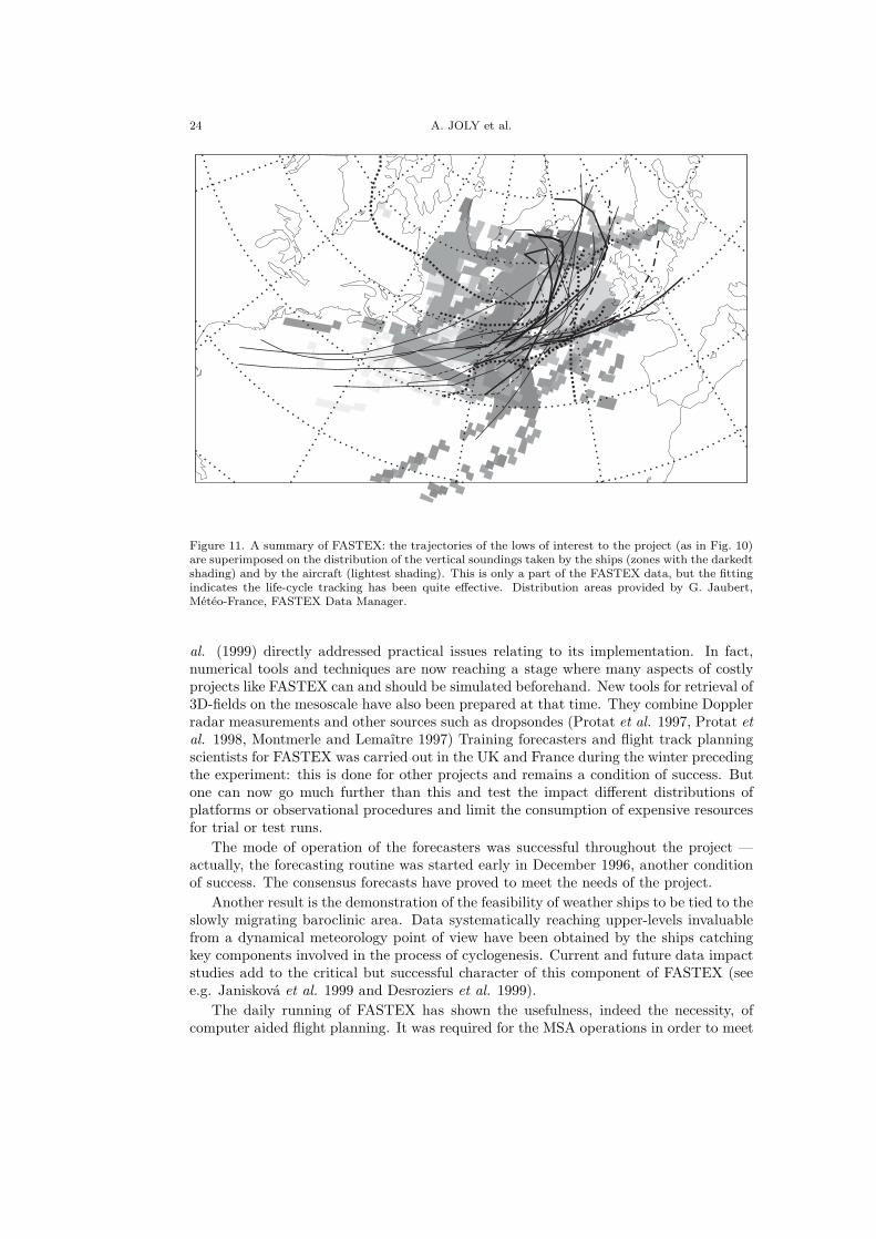
Figure 11. A summary of FASTEX: the trajectories of the lows of interest to the project (as in Fig. 10)are superimposed on the distribution of the vertical soundings taken by the ships (zones with the darkedtshading) and by the aircraft (lightest shading). This is only a part of the FASTEX data, but the fittingindicates the life-cycle tracking has been quite effective. Distribution areas provided by G. Jaubert,Météo-France, FASTEX Data Manager.

al. (1999) directly addressed practical issues relating to its implementation. In fact,numerical tools and techniques are now reaching a stage where many aspects of costlyprojects like FASTEX can and should be simulated beforehand. New tools for retrieval of3D-fields on the mesoscale have also been prepared at that time. They combine Dopplerradar measurements and other sources such as dropsondes (Protat et al. 1997, Protat etal. 1998, Montmerle and Lemaître 1997) Training forecasters and flight track planningscientists for FASTEX was carried out in the UK and France during the winter precedingthe experiment: this is done for other projects and remains a condition of success. Butone can now go much further than this and test the impact different distributions ofplatforms or observational procedures and limit the consumption of expensive resourcesfor trial or test runs.

The mode of operation of the forecasters was successful throughout the project —actually, the forecasting routine was started early in December 1996, another conditionof success. The consensus forecasts have proved to meet the needs of the project.

Another result is the demonstration of the feasibility of weather ships to be tied to theslowly migrating baroclinic area. Data systematically reaching upper-levels invaluablefrom a dynamical meteorology point of view have been obtained by the ships catchingkey components involved in the process of cyclogenesis. Current and future data impactstudies add to the critical but successful character of this component of FASTEX (seee.g. Janisková et al. 1999 and Desroziers et al. 1999).

The daily running of FASTEX has shown the usefulness, indeed the necessity, ofcomputer aided flight planning. It was required for the MSA operations in order to meet

OVERVIEW OF THE FIELD PHASE OF FASTEX 25

the multiple constraints: the intrinsic complexity of the reference flight patterns, theactual weather and the logistical and air safety regulations. It was found compulsory foroperating the Gulfstream because most objectives required its full range. (The computerprograms for the MSA were developed by the NSSL and JCMM groups, the one for theGulfstream by the Laboratoire d’Aérologie.)

Above all, the field phase of FASTEX as a whole has demonstrated the feasibility,despite the manifest difficulties, of a coordinated multi-base, multi-objectives observingsystem covering a whole ocean and closely associating scientists and meteorologists frommany different countries. This result is a nice example of scientific achievements thatwere made possible through the collaborative efforts of researchers working in differentareas but within the same field experiment, and for the same overall goal: improving ourunderstanding and forecasting ability of extratropical cyclones. One way of summarizingthe effectiveness of the tracking of the North-Atlantic cyclones is given by Fig. 11, wherethe overall distribution of the soundings taken from the FASTEX main platforms issuperimposed on the system trajectories: apart from the earliest phases of some of thecyclones, tracks and data distribution remarkably overlap throughout the ocean: fortwo-months, the Atlantic data gap has been filled.

Acknowledgment

This overview of the FASTEX field phase is dedicated to the many who were involvedin it in one way or another: in launching radiosondes at unsocial times and/or in remotelocations, monitoring logistical components of FASTEX such as money, goods and peo-ples’ movements, producing and disemminating special products from numerical modelsand remote sensors, maintaining computers and telecommunication lines, producing fore-casts, flying and maintaining aircraft, pushing back the limits of plans and regulations,and navigating and maintaining ships and their instruments in incredible conditions.

We also acknowledge constant and friendly support of the Aer Rianta staff in Shannonas well as the understanding of air traffic control authorities especially in Shannon,Prestwick, Gander and New-York.

FASTEX has been supported by the Programme Atmosphère et Océan à MoyenneEchelle of the Institut National des Sciences de l’Univers, Météo-France, IFREMER,CNES and other institutions under contract 97/02, by the European Commission un-der contract ENV4-CT96-0322, as well as by the National Science Foundation (USA),the National Oceanic and Atmospheric Administration (USA), the UK MeteorologicalOffice and the National Environment Research Council (UK), the World MeteorologicalOrganization and many national weather services.

Appendix A

This appendix provides the list of the acronyms used in the text, se Table A.1.

Appendix B

The following tables provide some reference data on the 25 FASTEX cases. A fewbasic meteorological characteristics are provided on the top rows. More detailed meteo-rological parameters can be found in Clough et al. (1998) or in Baehr et al. (1999). Therest of the table summarize the operations in the three FASTEX areas.

The labelling of the tables is self-explicit, except for the layout described in thefollowing table and regarding soundings:

26 A. JOLY et al.

TABLE A.1. List of acronymsAES Atmospheric Environment Service

(Canada)CETP Centre d’étude des Environnements

Terrestre et PlanétairesCMC Centre Météorologique Canadien,

Montréal, CanadaCNRS Centre National de Recherches Scien-

tifiquesCOSNA Composite Observing System for the

North-AtlanticEC European Commission

EGOS European Group on Ocean Stations FASTEX Fronts and Atlantic Storm-Track Ex-periment

FIC Flight International Company GPS Global Positioning SystemGTS Global Transmission System (operated

by WMO)INSU Institut National des Sciences de

l’UniversIOP Intensive Observation Period JCMM Joint Centre for Mesoscale Meteorol-

ogyJOSS Joint Office for Science Support LOP Lesser Observations Period (some-

times preceded by FASTEX)MIT Massachusetts Institute of Technology MSA Multiscale Sampling AreaNCAR National Center for Atmospheric Re-

searchNCEP National Center for Environmental

PredictionNESDIS National Environmental Satellite Data

and Information ServiceNOAA National Oceanic and Atmospheric Ad-

ministrationNRL Naval Reasearch Laboratory NSF National Science FoundationNSSL National Severe Storm Laboratory UCAR University Corporation for Atmo-

spheric ResearchUCLA University of California, Los Angeles UK United KingdomUSA United States of America WMO World Meteorological Organisation

Sounding information layout in Table B.1 andTable B.2

Ship name intensive duration number ofperiod of intensive profiles in

mid-time period Data Base

(Ship location)

Aircraft name flight duration number ofmid-time of flight dropsondes in

Data Base

In other words, for the special FASTEX platforms, the information is generally the middletime of the intensive period. For land radiosoundings, beginning and sometimes endperiods are specified. For the european radiosoundings, the number after the durationis the number of stations involved. The number of profiles refer to the high resolutionsoundings available in the data base in july 1999, as given by the data availability pages.

OVERVIEW OF THE FIELD PHASE OF FASTEX 27

TA

BLE

B.1

.T

he

FA

ST

EX

Inten

sive

Obs

erva

tio

nPer

iods

IOP

1IO

P2

IOP

3cy

clon

enu

mbe

r8A

1114

form

atio

nda

te8/

106

(54W

,41

N)

11/1

18(2

3W,40

N)

13/1

12(5

3W,41

N)

max

deep

enin

g8/

112

(47W

,42

N)

13/1

00(1

8W,53

N)

14/1

12(3

2W,43

N)

rate

(mba

r/6h

)-9

-10

-9

max

ampl

itud

e10

/100

(33W

,54

N)

13/1

00(1

5W,59

N)

15/1

18(2

9W,51

N)

(mba

r)96

8tlw

978

973

end

oftr

acki

ng11

/100

(40W

,55

N)

13/1

00(1

5W,59

N)

16/1

06(2

8W,58

N)

RS

US

8/1

18−→

−→12

/118

13/1

0614

/106

Lea

rJet

11/1

0345

1213

/104

3014

1500

1215

C13

0U

SAF

Gul

fstr

eam

(1)

KN

OR

R9/

124

910

/115

814

/124

1212

00(3

5W,42

N)

2230

(35W

,42

N)

1800

(35W

,45

N)

ÆG

IR9/

118

715

/118

909

00(3

5W,46

N)

0300

(35W

,49

N)

SUR

OÎT

9/1

242

10/1

154

14/1

1811

1200

(31W

,39

N)

2230

(34W

,41N

)09

00(4

1W,46

N)

V.B

UG

AE

V10

/136

1414

/118

1318

00(3

5W,3

8N)

0900

(35W

,42

N)

Oth

ersh

ips

11/1

2A

SAP

06-1

8G

ulfs

trea

m(2

)

C13

010

/107

3031

12/1

0945

4707

4515

00P

3N

OA

A10

/108

4012

/109

0006

3016

15E

lect

ra10

/105

00ss

12/1

0700

mi

0600

1615

Gul

fstr

eam

(3)

Eur

opea

nR

S10

/112

245

12/1

1224

516

/106

245

Oth

er

IOP

4IO

P5

IOP

618

19A

/B20

16/1

18(3

3W,47

N)

22/1

00(2

5W,47

N)

22/1

12(4

3W,46

N)

17/1

06(2

7W,47

N)

nosi

gnifi

cant

23/1

00(3

5W,50

N)

-2pr

essu

rede

epen

ing

-4

17/1

12(2

5W,48

N)

22/1

18(1

7W,44

N)

23/1

00(3

5W,50

N)

995

1008

984

18/1

06(1

5W,52

N)

23/1

06sp

litting

23/1

12(2

5W,57

N)

19/1

1820

/118

22/1

18

20/1

0445

1611

30

16/1

1813

20/1

1811

22/1

249

1500

(35W

,46

N)

2100

(48W

,45

N)

1200

(49W

,45

N)

16/1

1815

21/1

247

23/1

247

1500

(35W

,50

N)

0600

(35W

,52

N)

0300

(35W

,51

N)

16/1

1812

20/1

1811

23/1

247

1500

(43W

,47

N)

2100

(35W

,47N

)03

00(3

5W,49

N)

16/1

187

21/1

249

23/1

2410

1500

(35W

,42

N)

0600

(35W

,45N

)03

00(3

5W,45

N)

23/1

1A

SAP

22/1

0430

709

1522

/109

3013

4522

/106

00ss

1200

17/1

0645

2822

/103

150

23/1

0745

2212

1512

1519

4518

/118

245

22/1

1524

724

/103

246

19/1

0024

7

28 A. JOLY et al.

Tabl

eB

.1contin

ued

IOP

7IO

P8

IOP

9cy

clon

enu

mbe

r22

A/B

Gre

enla

ndle

ew

aves

27

form

atio

nda

te25

/112

(27W

,50

N)

30/1

12(7

8W,31

N)

max

deep

enin

g25

/106

(32W

,47

N)

Com

plex

inte

ract

ion

31/1

12(6

6W,37

N)

rate

(mba

r/6h

)<

1lo

w/o

rogr

aphy

-7

max

ampl

itud

e26

/100

(18W

,55

N)

3/2

06(1

8W,63

N)

(mba

r)tlw

1012

975

end

oftr

acki

ng26

/112

(15W

,55

N)

3/2

18(

2W,68

N)

RS

US

31/1

06−→

Lea

rJet

1/2

0330

1100

00C

130

USA

F27

/106

0013

0100

Gul

fstr

eam

(1)

1/2

0530

3011

45Sh

→St

JK

NO

RR

ÆG

IR25

/124

906

00(3

5W,49

N)

SUR

OÎT

25/1

248

29/1

506

00(3

5W,52

N)

(39W

,45N

)V

.B

UG

AE

V25

/124

82/

224

306

00(3

5W,45

N)

(56W

,44

N)

Oth

ersh

ips

Gul

fstr

eam

(2)

25/1

0630

2829

/107

1519

2015

1230

C13

026

/107

0041

0030

P3

NO

AA

26/1

0800

2/2

0900

501

0020

00ss

Ele

ctra

26/1

0600

ss2/

207

00m

i02

4523

00G

ulfs

trea

m(3

)

Eur

opea

nR

S26

/100

124

3/2

0318

5

Oth

erN

orss

arsu

aq1/

218

8

IOP

10IO

P11

IOP

1228

3034

3/2

12(4

0W,45

N)

4/2

06(6

0W,37

N)

9/2

06(3

5W,48

N)

4/2

12(1

7W,48

N)

5/2

06(3

9W,44

N)

9/2

12(2

7W,52

N)

-3-1

3-2

2

4/2

18(1

0W,50

N)

7/2

00(

5W,68

N)

10/2

06(2

0W,62

N)

1010

950

947

5/2

12(

5E,50

N)

7/2

00(

5W,68

N)

11/2

00(3

0W,65

N)

−→−→

−→4/

200

8/2

06−→

4/2

0330

168/

211

0011

1415

0545

(NB

:C13

0)2/

210

4519

4/2

0945

139/

207

307

1700

1615

1315

8/2

0530

2612

15Sh

→St

J6/

248

159/

224

800

00(5

1W,51

N)

1200

(51W

,56

N)

4/2

2410

6/2

2410

9/2

2412

1200

(12W

,50

N)

0300

(24W

,47

N)

1500

(35W

,46

N)

6/2

309

9/2

249

1200

(31W

,44N

)15

00(3

5W,50

N)

3/2

247

6/2

245

9/2

2414

0600

(50W

,43

N)

0300

(35W

,41N

)15

00(3

5W,41

N)

9/2

1A

SAP

3/2

0545

38St

J→

Sh18

15St

J→

Sh4/

209

0027

5/2

1000

709/

211

3043

0930

2300

1745

4/2

0915

16/

210

009/

210

00ss

1030

0145

1800

4/2

0730

ss5/

207

00ss

0915

2200

6/2

0530

4201

154/

203

2412

6/2

0618

410

/209

248

2A

RAT

fligh

ts4/

2

OVERVIEW OF THE FIELD PHASE OF FASTEX 29

Tabl

eB

.1contin

ued

IOP

13IO

P14

IOP

15cy

clon

enu

mbe

r35

/35A

3738

form

atio

nda

te8/

206

(85W

,32

N)

10/2

18(7

7W,28

N)

13/2

12(5

8W,42

N)

max

deep

enin

g9/

218

(62W

,39

N)

11/2

18(6

5W,37

N)

14/2

00(5

0W,46

N)

rate

(mba

r/6h

)-6

-9-1

0

max

ampl

itud

e10

/218

(43W

,46

N)

12/2

18(4

5W,43

N)

15/2

18(2

4W,53

N)

(mba

r)98

998

697

3

end

oftr

acki

ng13

/200

(2W

,59

N)

15/2

00(

3W,48

N)

17/2

18(3

8W,63

N)

RS

US

−→9/

218

11/2

0612

/206

13/2

0614

/200

Lea

rJet

10/2

0500

1912

/204

1523

14/2

0400

1911

0010

3013

30C

130

USA

F

Gul

fstr

eam

(1)

13/2

0500

014

30Sh

→St

JK

NO

RR

10/2

246

13/2

248

1200

(54W

,57

N)

1500

(55W

,59

N)

ÆG

IR10

/218

1013

/218

614

/224

721

00(3

5W,46

N)

0000

(35W

,46

N)

1800

(35W

,46

N)

SUR

OÎT

10/2

3018

13/2

187

14/2

246

2100

(35W

,52

N)

0000

(38W

,50N

)18

00(3

9W,50

N)

V.B

UG

AE

V10

/224

1513

/218

714

/224

721

00(3

5W,41

N)

0000

(35W

,41N

)18

00(3

5W,41

N)

Oth

ersh

ips

13/2

1A

SAP

15/2

1A

SAP

0606

Gul

fstr

eam

(2)

15/2

0630

3006

15St

J→

ShC

130

15/2

1100

4011

30P

3N

OA

A15

/208

30ss

1145

Ele

ctra

Gul

fstr

eam

(3)

Eur

opea

nR

S16

/215

92

Oth

er

IOP

16IO

P17

IOP

1839

A41

44

17/2

00(3

7W,49

N)

17/2

12(6

1W,3

5N)

22/2

12(4

4W,5

4N)

17/2

06(2

5W,52

N)

19/2

00(2

2W,51

N)

23/2

00(3

2W,53

N)

-20

-16

-10

18/2

06(1

2W,68

N)

20/2

00(7

W,62

N)

24/2

18(

4W,60

N)

943

943

950

18/2

06(1

2W,68

N)

20/2

00(7

W,62

N)

25/2

00(

4W,60

N)

15/2

12−→

−→18

/200

19/2

1822

/218

18/2

0245

1522

/204

0018

0015

0000

(17/

2)(0

6)17

/205

0022

22/2

0630

28Sh

→St

J17

3011

15Sh

→G

ob16

/224

818

/224

522

/224

812

00(5

3W,61

N)

1200

(51W

,62N

)06

00(5

7W,57

N)

16/2

156

19/2

189

23/2

247

2230

(35W

,52

N)

0000

(35W

,52

N)

0000

(28W

,60

N)

16/2

155

18/2

1815

23/2

249

2230

(38W

,48

N)

1800

(36W

,46N

)00

00(4

2W,48

N)

16/2

156

18/2

1815

23/2

246

2230

(35W

,41

N)

1800

(35W

,41N

)00

00(3

5W,41

N)

23/2

1A

SAP

0618

/207

0054

22/2

0445

3318

3018

45G

ob→

Sh17

/211

0045

19/2

1030

4607

3006

4517

/206

45ss

19/2

0900

ss23

/209

1522

0700

0730

1515

mi

19/2

0700

3720

3017

/218

2410

19/2

1524

1024

/209

3012

Nor

s’aq

18/2

1224

8N

ors’

aq22

/200

248

IOP

1946

B

26/2

12(3

8W,41

N)

27/2

06(2

3W,60

N)

-11

27/2

12(2

5W,62

N)

957

28/2

06(2

8W,58

N)

23/2

1827

/200

26/2

0345

1700

00

27/2

247

1200

(49W

,60

N)

26/2

1813

1500

(40W

,45

N)

27/2

1811

0000

(28W

,40

N)

27/2

1100

4207

30

27/2

0730

4813

4527

/218

245

30 A. JOLY et al.

TA

BLE

B.2

.T

he

FA

ST

EX

Les

ser

Obs

erva

tio

ns

Per

iods

LO

P1

LO

P2

LO

P3

cycl

one

num

ber

1033

35A

form

atio

nda

te10

/100

(37W

,40

N)

7/2

00(5

2W,40

N)

12/2

06(1

0W,54

N)

max

deep

enin

g11

/100

(22W

,53

N)

8/2

06(2

9W,50

N)

12/2

18(

4W,57

N)

rate

(mba

r/6h

)-6

-9-7

max

ampl

itud

e11

/112

(29W

,59

N)

9/2

06(

5W,64

N)

13/2

00(

2W,58

N)

(mba

r)97

398

597

7

MSA

loca

tion

11/1

06(2

0W,56

N)

8/2

18(1

5W,55

N)

12/2

06(1

0W,54

N)

end

oftr

acki

ng12

/112

(1W

,68

N)

9/2

12(

2E,64

N)

13/2

00(

2W,58

N)

Ups

trea

mda

taU

SR

SC

130

US

see

IOP

135/

210

3018

1300

C13

0U

S6/

210

0015

0730

Ship

s3

ship

s4

s/j

Kno

rr8

s/j

see

IOP

139/

1K

,Æ

,S

7/2

(49W

,51

N)

10/1

Ægi

r8

s/j

Bug

aev

8s/

j7/

2(3

0W,47

N)

10/1

(35W

,38

N)

Suro

ît7

s/j

8/2

(35W

,41

N)

Bug

aev

8s/

j(3

5W,41

N)

Eur

ope,

MSA

Eur

oR

S→

11/1

12G

ulfs

trea

mda

ta8/

205

3026

1215

enro

ute

LO

P4

LO

P5

LO

P6

39B

42B

43A

17/2

06(4

5W,48

N)

22/2

06(2

7W,47

N)

24/2

00(3

3W,47

N)

17/2

18(2

0W,50

N)

22/2

12(2

1W,51

N)

24/2

12(1

6W,49

N)

-7-1

0-1

0

17/2

18(

9E,57

N)

23/2

12(

1E,63

N)

25/2

06(1

0E,57

N)

990

967

965

17/2

18(2

0W,50

N)

22/2

18(1

5W,54

N)

24/2

12(1

6W,49

N)

19/2

00(1

0E,58

N)

23/2

12(

1E,63

N)

25/2

06(1

0E,57

N)

US

RS

US

RS

US

RS

Lea

rJet

Lea

rJet

16/2

0830

2122

/202

0010

1345

2300

3sh

ips

5s/

j3

ship

s4

s/j

Suro

ît8

s/j

17/2

K,Æ

,B

21/2

Æ,S,

B23

/2(4

3W,47

N)

24/2

Bug

aev

4s/

j24

/2(3

5W,41

N)

Eur

oR

S→

18/2

18G

ulfs

trea

mE

uro

RS

→25

/218

22/2

0445

1845

enro

ute

OVERVIEW OF THE FIELD PHASE OF FASTEX 31

References

Appenzeller, Ch., 1994 Wave developments on surface fronts and stratospheric in-trusions. PhD thesis, Swiss Federal Institute of Tech-nology (ETH). Dissertation No 10471, 117pp.

Arbogast, Ph. and Joly, A., 1998 Identification des précurseurs d’une cyclogenèse.Compte-Rendus à l’Académie des Sciences, Sci-ences de la Terre et des planètes , 326, 227–230.

Ayrault, F., 1998 Environnement, structure et évolution des dépressionsmétéorologiques: réalité climatologique et modèlestypes. PhD thesis, Doctorat de Université P. Sabatier,Toulouse. 328pp.

Ayrault, F., Lalaurette, F.,Joly, A. and Loo, C.,

1995 North Atlantic Ultra-High Frequency variability: an intro-ductory survey. Tellus, 47A, 671–696.

Baehr, Ch., Pouponneau, B.,Ayrault, F. and Joly, A.,

1999 Dynamical characterization and summary of the FASTEXcyclogenesis cases. Q. J. R. Meteorol. Soc. , 125,revised version submitted.

Bergot, T., 1999 Adaptive observations during FASTEX: a systematic sur-vey of the impact of upstream flights. Q. J. R. Mete-orol. Soc. , 125, accepted.

Bergot, T., Hello, G., Joly, A.and Malardel, S.,

1999 Adaptive observations: a feasability study. Mon. WeatherRev. , 127, (5), 743–765.

Beugin, R. and Rochard, M., 1991 L’hiver 1989–1990. Les tempêtes et quelques autresphénomènes. Technical Report, Meteo-France,SCEM, Prévision générale et aéronautique. 184pp.

Bishop, C.H. and Thorpe, A.J., 1994 Frontal wave stability during moist deformation frontoge-nesis. part I. linear wave dynamics. J. Atmos. Sci. ,51, (6), 852–873.

Bishop, C.H. and Toth, Z., 1999 Ensemble transformation and adaptive observations. J.Atmos. Sci. , 56, (11), 1748–1765.

Bouniol, D., Protat, A. andLemaître, Y.,

1999 Mesoscale dynamics of a deepening secondary cyclone(FASTEX IOP 16): three-dimensional structure re-trieved from dropsonde data. Q. J. R. Meteorol. Soc. ,125, accepted.

Browning, K.A., 1994 GEWEX Cloud System Study (GCSS): science plan. Vol-ume 11, IGPO Publication Series. 62pp.

Cammas, J.P.,Pouponneau, B.,Desroziers, G.,Santurette, P., Joly, A.,Arbogast, Ph., Mallet, I.,Caniaux, G., Mascart, P.and Shapiro, M.,

1999 Initiation, triggering and development phases of theFASTEX cyclone (IOP 17): synoptic and dynamicoverview. Q. J. R. Meteorol. Soc. , 125, accepted.

Chaboureau, J.P. andThorpe, A.J.,

1999 Frontogenesis and the development of secondary wave cy-clones in FASTEX. Q. J. R. Meteorol. Soc. , 125,925–940.

Charney, J.G. and Stern, M.E., 1962 On the stability of internal baroclinic jets in a rotatingatmosphere. J. Atmos. Sci. , 19, 159–162.

Clough, S.A., Lean, H.W.,Roberts, N.M., Birkett, H.,Chaboureau, J.P.,Dixon, R., Griffiths, M.,Hewson, T.D. andMontani, A.,

1998 A JCMM overview of FASTEX IOPS. Technical Re-port 81, Joint Centre for Mesoscale Meteorology, Read-ing, UK.

Desroziers, G.,Pouponneau, B.,Thépaut, J.N.,Janisková, M. andVeersé, F.,

1999 Four dimensional variational analyses of FASTEX situa-tions. part II: use of additional observations. Q. J. R.Meteorol. Soc. , 125, accepted.

Eady, E.T., 1949 Long-waves and cyclone waves. Tellus , 1, (3), 33–52.

32 A. JOLY et al.

Eymard, L., Caniaux, G.,Dupuis, H., Prieur, L.,Giordani, H., Troadec, R.and Bourras, D.,

1999 Surface fluxes in the North-Atlantic Current during theCATCH/FASTEX experiment. Q. J. R. Meteorol.Soc. , 125, accepted.

Farrell, B.F., 1984 Modal and non-modal baroclinic waves. J. Atmos. Sci. ,41, (4), 668–673.

Farrell, B.F., 1990 Small error dynamics and the predictability of atmosphericflows. J. Atmos. Sci. , 47, (20), 2409–2416.

Fischer, C., Joly, A. andLalaurette, F.,

1998 Error growth and kalman filtering within an idealized baro-clinic flow. Tellus, 50A, (5), 596–615.

Gelaro, R., Langland, R. andRohaly, G.D.,

1999 An assessment of the singular vector approach to targetedobserving using the FASTEX data set. Q. J. R. Me-teorol. Soc. , 125, accepted.

Hadlock, R. andKreitzberg, C.W.,

1988 The Experiment on Rapidly Intensifying Cyclones over theAtlantic (ERICA) field study: objectives and plans.Bull. Amer. Meteorol. Soc. , 69, (11), 1309–1320.

Hello, G., Lalaurette, F. andThepaut, J.N.,

1999 Combined use of sensitivity information and observationsto improve meteorological forecast : the ChristmasStorm case. Q. J. R. Meteorol. Soc. , 125, (-), sub-mitted.

Hewson, T.D., 1997 Objective identification of frontal wave cyclones. Meteorol.Appl. , 4, 311–315.

Janisková, M., Veersé, F.,Thépaut, J.N.,Desroziers, G. andPouponneau, B.,

1999 Four dimensional variational analyses of FASTEX situa-tions. part I: impact of a simplified physical packagein the assimilating model. Q. J. R. Meteorol. Soc. ,125, accepted.

Jarraud, M., Goas, J. andDeyts, C.,

1989 Prediction of an exceptional storm over france and south-ern england (15–16 october 1987). Weather and Fore-casting, 4, 517–536.

Jaubert, G., Piriou, C.,Loehrer, S.M., Petitpa, A.and Moore, J.A.,

1999 The FASTEX experiment data archive. Q. J. R. Meteorol.Soc. , 125, accepted.

Joly, A., 1995 The stability of steady fronts and the adjoint method :non-modal frontal waves. J. Atmos. Sci. , 52, (17),3082–3108.

Joly, A., Jorgensen, D.,Shapiro, M.A.,Thorpe, A.J.,Bessemoulin, P.,Browning, K.A.,Cammas, J.P.,Chalon, J.P., Clough, S.A.,Emanuel, K.A.,Eymard, L., Gall, R.,Hildebrand, P.H.,Langland, R.H.,Lemaitre, Y., Lynch, P.,Moore, J.A.,Persson, P.O.G., Snyder, C.and Wakimoto, R.M.,

1997 The Fronts and Atlantic Storm-Track Experiment (FAS-TEX): scientific objectives and experimental design.Bull. Amer. Meteorol. Soc. , 78, (9), 1917–1940.

Kurz, M., 1995 synoptic-scale waves , in Images in weather forecasting,M.J. Bader, G.S. Forbes, J.R. Grant, R.B.E. Lilley,A.J. Waters eds, Cambridge University Press, 1995.187–200.

Langland, R.H., Gelaro, R.,Rohaly, G.D. andShapiro, M.A.,

1999 Targeted observations in FASTEX: adjoint-based tar-geting procedures and data impact experiments inIOPs-17 and 18. Q. J. R. Meteorol. Soc. , 125, ac-cepted.

Malardel, S., Joly, A.,Courbet, F. andCourtier, Ph.,

1993 Non-linear evolution of ordinary frontal waves induced bylow-level potential vorticity anomalies. Q. J. R. Me-teorol. Soc. , 119, 681–713.

OVERVIEW OF THE FIELD PHASE OF FASTEX 33

Mallet, I., Arbogast, Ph.,Baehr, Ch., Cammas, J.P.and Mascart, P.,

1999a Effects of a low level precursor and frontal stability on cy-clogenesis during FASTEX IOP17. Q. J. R. Meteorol.Soc. , 125, accepted.

Mallet, I., Cammas, J.P.,Mascart, P. andBechtold, P.,

1999b Effects of cloud diabatic heating on the FASTEX cyclone(IOP 17) early development. Q. J. R. Meteorol. Soc. ,125, accepted.

Marshall, J. and The Lab SeaGroup,

1998 The Labrador Sea Deep Convection Experiment. Bull.Amer. Meteorol. Soc. , 79, (10), 2033–2058.

Montmerle, T. andLemaître, Y.,

1997 Three-dimensional variational data analysis to retrievethermodynamical and dynamical fields from variousnested measurements. J. Atmos. Oceanic Technol. ,15, 360–379.

Orlanski, I. and Sheldon, J., 1995 Stages in the energetics of baroclinic systems. Tellus ,47A, 605–628.

Parsons, D.B. and Hobbs, P.V., 1983 The mesoscale and microscale structure and organisationof clouds and precipitation in midlatitudes cyclones.XI:comparisons between observational and theoreticalaspects of rainbands. J. Atmos. Sci. , 40, 2377–2397.

Protat, A., Lemaître, Y. andScialom, G.,

1997 Retrieval of kinematic fields using a single beam airbornedoppler radar performing circular trajectories. J. At-mos. Oceanic. Technol. , 14, 769–791.

Protat, A., Lemaître, Y. andScialom, G.,

1998 Thermodynamic analytical fields from Doppler radar databy means of the MANDOP analysis. Q. J. R. Meteo-rol. Soc. , 124, 1633–1669.

Pu, Z.X. and Kalnay, E., 1999 Targeting experiments with the quasi-inverse linear and ad-joint NCEP global model: the performance and evalu-ation during FASTEX. Q. J. R. Meteorol. Soc. , 125,accepted.

Ryan, B.F., 1996 On the global variation of precipitating layer clouds. Bull.Amer. Meteorol. Soc. , 77, (1), 53–70.

Sanders, F. and Gyakum, J.R., 1980 Synoptic-dynamic climatology of the “bomb”. Mon.Weather Rev. , 108, 1589–1606.

Schär, C. and Davies, H.C., 1990 An instability of mature cold front. J. Atmos. Sci. , 47,(8), 929–950.

Snyder, C., 1996 Summary of an informal workshop on adaptive observa-tions and FASTEX. Bull. Amer. Meteorol. Soc. , 77,(5), 953–961.

Stewart, R.E., 1991 Canadian Atlantic Storms Program: progress and plans ofthe meteorological component. Bull. Amer. Meteorol.Soc. , 72, (3), 364–371.

Stewart, R.E., Szeto, K.K.,Reinking, R.F.,Clough, S.A. andBallard, S.P.,

1998 Midlatitude cyclonic cloud systems and their featuresaffecting large scales and climate. Reviews of Geo-physics, 36, (2), 245–273.

Szunyogh, I., Toth, Z.,Emanuel, K.A.,Bishop, C.H., Snyder, C.,Morss, R., Woolen, J. andMarchok, T.,

1999 Ensemble-based targeting experiments during fastex: theimpact of dropsonde data from the Learjet. Q. J. R.Meteorol. Soc. , 125, accepted.

Thorncroft, C.D. andHoskins, B.J.,

1990 Frontal cyclogenesis. J. Atmos. Sci. , 47, (19), 2317–2336.

Uccellini, L.W., Kocin, P.J.,Petersen, R.A., Wash, C.H.and Brill, K.F.,

1984 The President’s Day cyclone of 18–19 February 1979:synoptic overview and analysis of the subtropical jetstreak influencing the precyclogenetic period. Mon.Weather Rev. , 112, 31–55.

Vautard, R., Legras, B. andDéqué , M.,

1988 On the source of midlatitude low-frequency variability.part I: a statistical approach to persistence. J. Atmos.Sci. , 45, (20), 2811–2843.

This file has been processed by LATEX2ε with the package qjrms2e.sty developed at Météo-France