overview of landscape dynamic concepts - home | … of landscape dynamic concepts instructor: k....

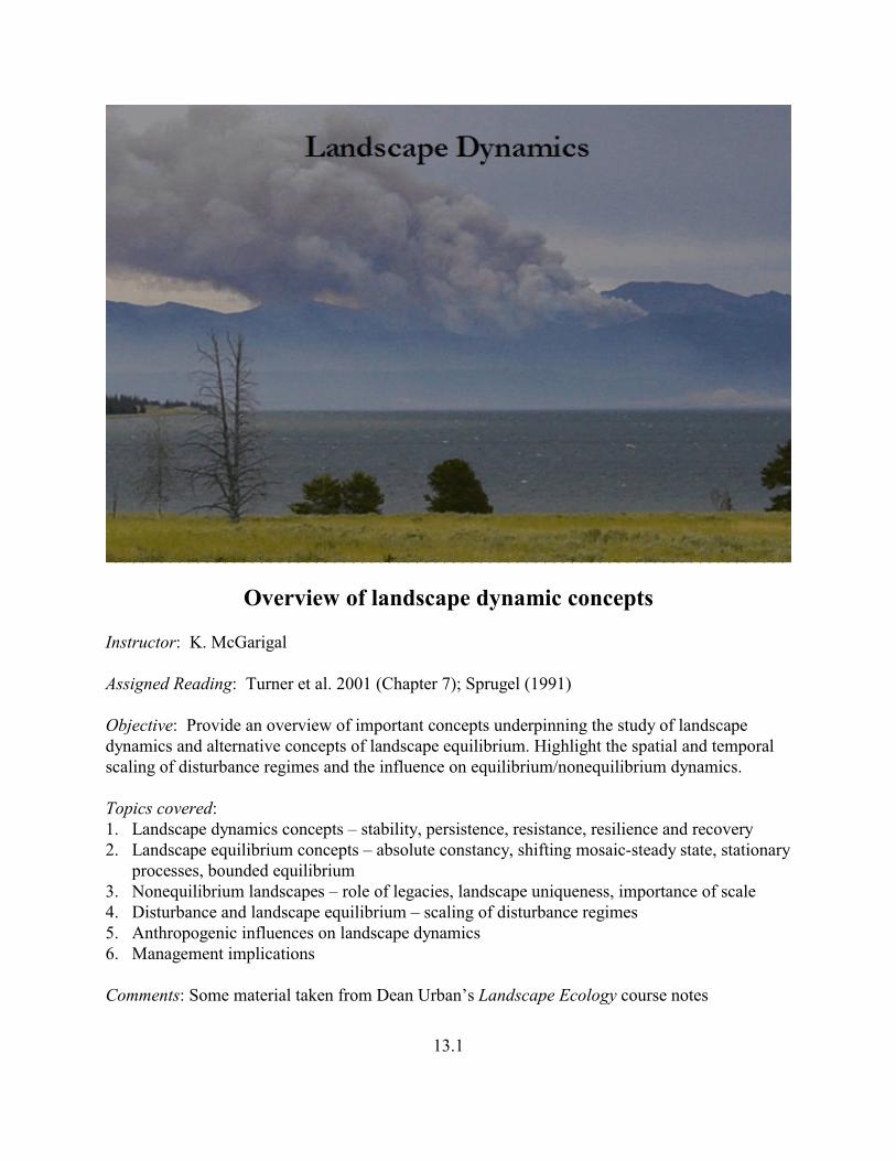
Overview of landscape dynamic concepts

Instructor: K. McGarigal

Assigned Reading: Turner et al. 2001 (Chapter 7); Sprugel (1991)

Objective: Provide an overview of important concepts underpinning the study of landscapedynamics and alternative concepts of landscape equilibrium. Highlight the spatial and temporalscaling of disturbance regimes and the influence on equilibrium/nonequilibrium dynamics.

Topics covered:1. Landscape dynamics concepts – stability, persistence, resistance, resilience and recovery2. Landscape equilibrium concepts – absolute constancy, shifting mosaic-steady state, stationary

processes, bounded equilibrium3. Nonequilibrium landscapes – role of legacies, landscape uniqueness, importance of scale4. Disturbance and landscape equilibrium – scaling of disturbance regimes5. Anthropogenic influences on landscape dynamics6. Management implications

Comments: Some material taken from Dean Urban’s Landscape Ecology course notes

13.1

1. Landscape Dynamics Concepts

For heuristic purposes, a simple conceptual framework for discussing ecosystem/landscapedynamics is needed. In this simple model, we depict system dynamics as a trajectory over time ina state variable. A state variable is any variable the describes the state or condition of the systemat a single point in time and is typically a measure of system structure or function. For example,the percentage of the landscape in a particular vegetation condition, mean patch size, total waterdischarge, and net primary productivity are all examples of potential state variables. As shownhere, under a “natural” disturbance regime, the trajectory in a state variable might fluctuate overtime in response to disturbance and succession processes and vary within a “natural range ofvariability”, or what is sometimes referred to as the “normal multiple states operating range”.Note, this range of variability is relative to a specific spatial and temporal scale.

13.2

This model provides a simple reference framework for assessing the effects of human activitieson system dynamics. For example, in this figure, two alternative human-altered trajectories aredepicted, and we might ask whether the system depicted by each trajectory is “healthy” inreference to the natural range of variability. In both cases, the system dynamics are substantiallymodified; specifically, the dynamics are substantially dampened. In the one case, the systemremains within its natural range of variability, while in the other case, the system moves to anequilibrium state outside of its natural range of variability. In both cases, we might ask whetherthe trajectory depicts a “healthy” system. This is not an easy question to answer in either case.

13.3

Any consideration of system dynamics automatically invokes issues of scale because the range ofvariability in any state variable can only be defined in reference to a specific spatial and temporalscale. For example, as the spatial extent of the system gets larger and larger (i.e., coarser scale),the expected range of variability is likely to decrease as the system increasingly is able toincorporate the disturbances; i.e., balance of disturbance against succession (sensu Watt’s unitpattern).

13.4

Defining this scaling relationship for a natural system is of interest to us of course, but perhaps ofeven greater interest is how this scaling relationship changes under a human-modifieddisturbance regime. For example, if the human-altered trajectory looks like the one depicted here(i.e., the range of variability is increasingly dampened as the spatial scale increases), we mightask whether this is a healthy system?

13.5

Understanding system dynamics has utility in a wide range of applications. For example, aquestion of great importance to resource managers is whether recent trends in wildlifepopulations and/or habit are biologically significant and signal the need for correctivemanagement action. If the trajectory is decreasing (e.g., population decrease), for example,managers are often quick to interpret this as a signal for immediate management action.However, an understanding of system dynamics may reveal that the decrease is perfectly naturaland well within the range of natural variation.

13.6

And as we have already discussed, a quantitative understanding of system dynamics can bevitally important in providing a reference framework for interpreting measures of landscapestructure. Recall that it is often difficult, if not impossible, to determine the ecologicalsignificance of the computed value of a landscape metric without understanding its natural rangeof variability.

13.7

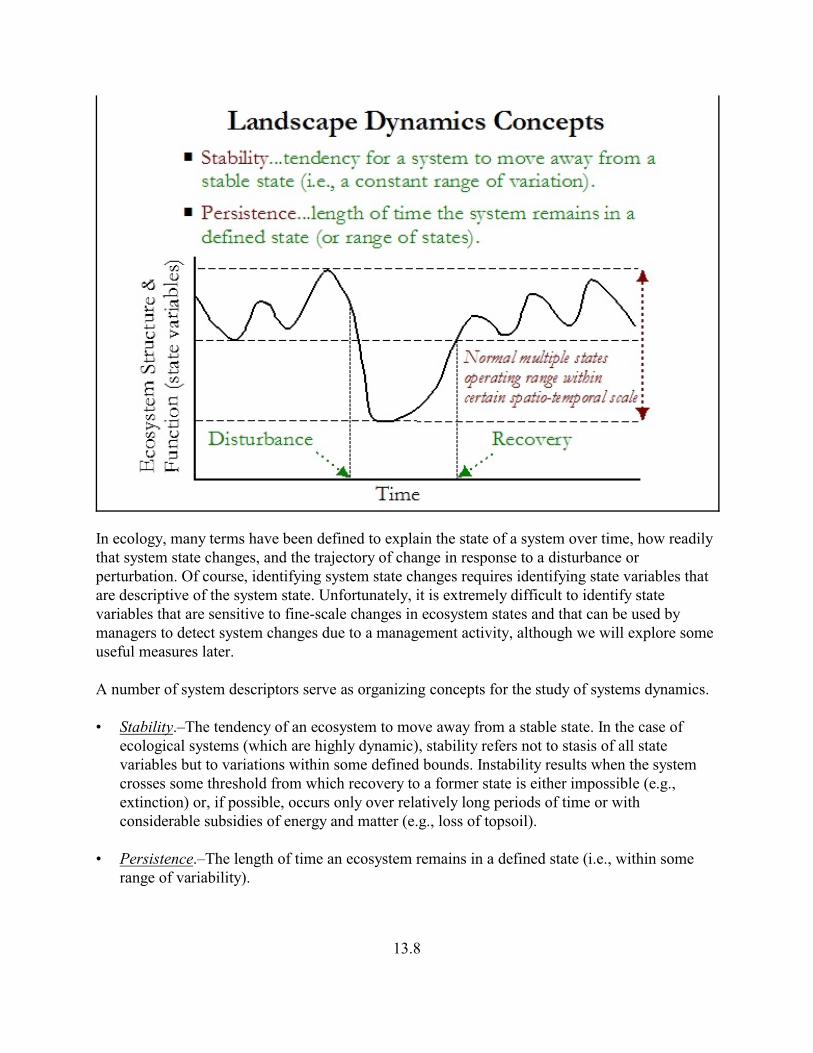
In ecology, many terms have been defined to explain the state of a system over time, how readilythat system state changes, and the trajectory of change in response to a disturbance orperturbation. Of course, identifying system state changes requires identifying state variables thatare descriptive of the system state. Unfortunately, it is extremely difficult to identify statevariables that are sensitive to fine-scale changes in ecosystem states and that can be used bymanagers to detect system changes due to a management activity, although we will explore someuseful measures later.

A number of system descriptors serve as organizing concepts for the study of systems dynamics.

• Stability.–The tendency of an ecosystem to move away from a stable state. In the case ofecological systems (which are highly dynamic), stability refers not to stasis of all statevariables but to variations within some defined bounds. Instability results when the systemcrosses some threshold from which recovery to a former state is either impossible (e.g.,extinction) or, if possible, occurs only over relatively long periods of time or withconsiderable subsidies of energy and matter (e.g., loss of topsoil).

• Persistence.–The length of time an ecosystem remains in a defined state (i.e., within somerange of variability).

13.8

• Resistance.–The capacity of an ecosystem to adsorb or otherwise dissipate perturbations andprevent them from amplifying into large disturbances. Resistance mechanisms may bethought of as filters that reduce the potential for large disturbances or as those properties–ofsystems and individuals–that maintain relative constancy in processes and that preventorganisms from succumbing to some stress.

13.9

• Resilience.–The capacity of an ecosystem to return to the preperturbation state following adisturbance. Refers to the bounds in state space around which a system will vary but return topreperturbation state. If the system moves outside these bounds, it will move to another state.While the state to which the system recovers is unlikely to be an exact replica of what existedbefore, it nevertheless contains the same basic elements (species richness, habitats, soilfertility) and supports the same key processes (e.g., photosynthetic capacity and nutrient andhydrologic cycles). In other the words, system integrity is maintained.

• Recovery.–The speed with which an ecosystem returns to the preperturbation state followinga disturbance.

13.10

It is worth noting that stability per se can be achieved in ecosystems in several different ways:

1. In systems that can be altered relatively easily (i.e., low resistance) but will return to theinitial state rapidly (i.e., rapid recovery and high resiliance). Such systems are oftencharacterized by low biomass.

2. In systems that maintain ahigh resistance todisturbance and thus persistin a stable state for longperiods of time. Suchsystems are oftencharacterized by highbiomass.

3. Physical system stabilitycan be achieved in certainecosystems. Such systemsare characterized by theabsence of biomass.

13.11

2. Landscape Equilibrium Concepts

Turner et al. (1993) reviewed several concepts of landscape equilibrium.

2.1. Absolute Constancy

The simplest concept of order that might be imposed on a landscape would be equilibrium in thesense of absolute constancy; that is, there are no changes through time. Clearly, however,disturbances and change are integral parts of landscape dynamics and make this notion ofequilibrium unrealistic.

13.12

2.2. Shifting Mosaic Steady-State

In the shifting mosaic steady-state concept (Bormann and Liken 1979), the vegetation present atindividual points on the landscape changes, but, if averaged over a sufficiently long time or largearea, the proportion of the landscape in each seral stage is relatively constant, i.e., is inequilibrium (sensu Watt’s unit pattern). This concept emphasizes that even systems with a highdisturbance frequency could be in a ‘steady-state’ or ‘equilibrium’ if the creation of new patchesis balanced by the maturation of old ones (i.e., balance between disturbance and succession on alarger scale).

13.13

The shifting mosaic steady-state concept has been difficult to test empirically, but it has beensuggested to apply to some systems.

• Northern hardwood forests of New England.–predominant disturbance is windthrow ofindividual trees or small groups, resulting in a stable patchwork of gaps in various phases ofsuccession (i.e., gap-phase succession), at the scale of a small watershed.

• Balsam fir forests of the northeastern U.S.–wave-regenerated forests, where natural‘mortality waves’ move through the forest once every 50-70 years. Since the waves move at afairly uniform rate, there are always freshly killed areas, and since consecutive waves are onlyabout 100 m or so apart, an area of a few dozen hectares will normally contain all phases ofthe disturbance cycle.

These systems are said to be in equilibrium or quasi-equilibrium because disturbance issufficiently frequent and small-scale compared to the landscape area that most populations andprocesses are fairly constant over the whole area.

13.14

The shifting mosaic steady-state concept is problematic as a general property of landscapes forseveral reasons.

• The concept is applicable only when disturbances are small and frequent in a large area ofhomogeneous habitat. Thus, large areas may be more likely than small areas to exhibit astable mosaic. Few studies have identified stable mosaics even over relatively large areas.

13.15

• The concept assumes that the effects of discontinuities or gradients in topography, soils,moisture or other factors that would affect disturbance frequency or recovery are averagedacross the landscape. This is a difficult condition to satisfy on real landscapes.

13.16

• The concept is scale-dependent. Defining the sufficiently broad temporal and spatial scalesover which to consider the aggregate mosaic is ambiguous. Equilibrium conditions do notexist at extremely fine and extremely coarse scales. It is conceivable to find a shifting steady-state mosaic on some landscapes at some intermediate scales, but it is difficult to specify therelevant spatial and temporal scale a priori.

13.17

2.3. Stationary Process

Another concept considers landscape equilibrium to be a stationary process with randomperturbation. A stationary process is a stochastic process that does not change in distribution overtime or space.

Loucks (1970) suggested that communities may appear unstable at any particular point in timebecause community composition is changing, but that the entire long-term sequence of changesconstitutes a stable system because the same sequence recurs after every disturbance.

In fire-dominated landscapes, the statistical distribution of seral stages, fire return intervals, firesizes, or similar parameters can be determined. This stationary process concept explicitlyacknowledges the stochastic nature of disturbance, e.g., consider a probability density functionfor fire return intervals, but assumes that the distribution of fire return intervals (e.g., a negativeexponential) remains more or less constant through time. Thus, the fire return interval may vary,and the probability of fire return may change with time since last disturbance, but when averagedover a sufficient large landscape and over a sufficiently long period of time, the statisticaldistribution remains relatively constant.

13.18

Unfortunately, the stationary process concept cannot escape the problems of scale discussed forthe shifting mosaic steady-state concept. As with the steady-state, the stationary distributioncannot be achieved at extremely fine and extremely coarse scales, and it is difficult to specify therelevant spatial and temporal scale a priori.

13.19

2.4. Bounded Equilibrium

A concept related to the stationary process is that of stochastic or relative constancy throughtime. In this scenario, the system exhibits random changes (e.g., in response to stochasticdisturbance events) but remains within bounds.

Unfortunately, the concept of a bounded equilibrium concept cannot escape the problems ofscale. For example, long-term monotonic changes in climate due to global warming or glacialcycles would eventually move the landscape out of pre-set bounds. And not even reasonablebounds are sufficient to envelop a spatial extent larger than a biome.

13.20

2.5. Homeorhetic Stability

With most concepts, equilibrium has been defined relative to some “undisturbed” state. Alandscape has been considered as being in equilibrium if it remains in the neighborhood of someundisturbed state or remains balanced in the recovery stages leading to this undisturbed state.However, communities are in a constant dynamic process of adaptation to their environment suchthat stability in this sense may be unrealistic.

A more appropriate concept of stability may be that of ‘homeorhetic’ stability, which states thatif perturbed, a system returns to its preperturbation trajectory or rate of change. Homeorheticstability implies return to normal dynamics rather than return to an artificial “undisturbed” state.

13.22

3. Equilibrium or Nonequilibrium landscapes? – role of legacies, landscapeuniqueness, and the importance of scale

Sprugel (1991) reviewed several examples of systems thought to be exemplary of the balance ofnature in a "natural" state, including the African savanna, the "Big Woods" of Minnesota,lodgepole pine landscapes of the Yellowstone area, and old-growth forests in the PacificNorthwestern United States. He noted that in some areas an equilibrium may exist inwhich patchy disturbance is balanced by regrowth, but in others equilibrium may be impossiblebecause (1) individual disturbances are too large or infrequent; (2) ephemeral events havelong-lasting disruptive effects; and/or (3) climate changes interrupt any movement towardequilibrium that does occur.

13.23

Based on these and other examples, Sprugel concluded the following:

• "Natural" vegetation is far less stable than it may seem to be from our human perspective; inparticular, all of the examples cited are transient or nonequilibrium over time scales measuredin life-times of the dominant organisms.

• Vegetation may preserve small or transient effects for a very long time, especially in the caseof forests of long-lived trees.

• "Every point in time is special" in that, at any time, vegetation has some characteristics thatdistinguish it from the same system at any other time.

• Thus, it may be impossible (or irrelevant) to define the "natural state of the system" -- formany if not most systems.

13.26

Clearly, the concept of balance is unrealistic if balance is interpreted as “no change.” However, ifwe take balance to mean that some changes in the state of a system are consistent withmaintaining species and processes, while other changes are not, then there clearly are balances innature, and different kinds of disturbances can have quite different implications for the integrityof natural and managed systems.

While nature is dynamic, not all changes are consistent with maintaining system integrity. Numerous examples can be cited of changes in system state (e.g., species composition andprocesses) that are quite distinct from normal successional changes; in essence, sites convert to anew community that itself may be self-reinforcing. Perhaps the most widely knowncontemporary examples are the collapse of some forests due to excessive pollution and theworldwide desertification of arid grasslands, a phenomenon underlain by loss of soil integrity dueto the combined effects of overgrazing and drought, exacerbated in many cases by an intensifieddisturbance regime due to the spread of flammable exotic grasses.

13.27

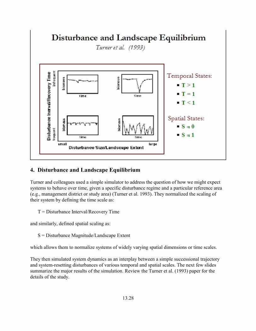
4. Disturbance and Landscape Equilibrium

Turner and colleagues used a simple simulator to address the question of how we might expectsystems to behave over time, given a specific disturbance regime and a particular reference area(e.g., management district or study area) (Turner et al. 1993). They normalized the scaling oftheir system by defining the time scale as:

T = Disturbance Interval/Recovery Time

and similarly, defined spatial scaling as:

S = Disturbance Magnitude/Landscape Extent

which allows them to normalize systems of widely varying spatial dimensions or time scales.

They then simulated system dynamics as an interplay between a simple successional trajectoryand system-resetting disturbances of various temporal and spatial scales. The next few slidessummarize the major results of the simulation. Review the Turner et al. (1993) paper for thedetails of the study.

13.28

Briefly, Turner and colleagues concluded the following:

• Characteristic dynamics can be predicted from the relative scaling of the disturbance regime.• Disturbance-driven landscapes might be equilibrium, quasi-equilibrium, or inherently

nonequilibrium (or combo's of these). • Anthropogenic influences may rescale these and change the qualitative dynamics of systems

(e.g., fire suppression rescales a fire regime).

13.31

5. Anthropogenic Influences on Landscape Dynamics

Much of the interest in landscape dynamics is stimulated by the desire to understand how humanactivities have influenced landscapes, and how this understanding can inform land planning.Much of the focus has been on how anthropogenic changes in disturbance regimes have alteredlandscape patterns and dynamics. In particular, changes in fire disturbance regimes due to alteredclimate conditions or fire suppression activities, and the impacts of forest management activities,particularly logging, have received the most attention. Historical retrospective studies and spatialmodeling have combined to provide important insights.

• Changing disturbance regimes can have an immediate effect on some measures of landscapepattern, no effect on others, and a significantly delayed effect on others. For example, Baker(1992) modeled the effect of human settlement and fire suppression on landscape structure inthe Boundary Waters Canoe area in northern Minnesota. Settlement produced immediateeffects on some metrics, including patch age, patch shape, and Shannon’s diversity, but noeffect on others, including patch size and fractal dimension. Fire suppression resulted inimmediate responses in a few metrics, but a delay of several decades in patch age and fractaldimension and a delay for hundreds of years in others, including patch size. Thus, the effectsof changes in disturbance regime may not be observed for many years, making it difficult todocument the impacts.

13.32

• Altered disturbance regimes can have a long-lasting ‘legacy’ effect on landscape dynamics;that is, human-altered disturbance regimes can have an impact on landscape pattern dynamicsthat may persist long after the disturbance regime has returned to ‘normal’. For example,Wallin et al. (1994) modeled changes in landscape structure in response to alternativeanthropogenic (forest cutting) disturbance regimes. This study was motivated by the questionof how long a pattern imposed by a particular forest cutting pattern would persist once thedisturbance regime was changed, for example, if forest harvest was to cease or if returnintervals were to be lengthened considerably.

13.33

Their results demonstrated that the landscape pattern created by dispersed disturbances wasdifficult to erase without a substantial reduction in disturbance rate or reduction in theminimum stand age eligible for disturbance. Even after only 20 yr of dispersed cutting, theswitch to aggregated cutting produced only small changes in landscape patterns as reflectedby edge density and mean size of interior forest patches; after 40 or 60 years of dispersedcutting, the change in disturbance regime produced an even smaller effect. This studydemonstrated that the response of landscape pattern can lag substantially behind a change inthe disturbance regime.

13.34

• In the same study, Wallin et al. (1994) also demonstrated a more general impact of alternativeforest cutting scenarios on the dynamics in landscape structure. Specifically, they conducted ahistorical reconstruction of vegetative cover classes dating back to 1560 in two watersheds inthe westside Cascade Mountains in Oregon. In addition, they simulated several alternative,but realistic, forest cutting scenarios under debate at the time by forest managers and policymakers. In addition to the rather obvious result that more intensive cutting regimes resulted inless mature, closed-canopy forest being sustained on the landscape over time, they alsodemonstrated the potential for all cutting scenarios to dramatically alter the dynamic behaviorof the landscape. Specifically, under all cutting scenarios, which involved completeregulation of the forest, the variability in landscape structure over time was severelydampened or eliminated compared to the historic range of variability (as defined), thusdramatically altering the landscape dynamics. While several scenarios maintained thelandscape structure within its historic range of variability, the ecological impacts of removingthe dynamic behavior of the landscape was less clear.

13.35

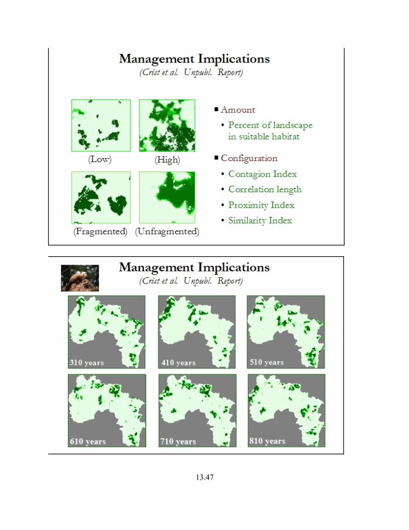
6. Management Implications

Understanding the dynamics of a landscape has numerous management implications. Here, wewill consider just a few.

• While managing for a stationary pattern may seem appealing from a purely pragmaticstandpoint, the simple fact is that in most real landscapes a stationary pattern is unlikely to beattained, and certainly cannot be sustained over time. Knowing the natural range of variabilityfor a system can put bounds on expected dynamics -- so we can temper our expectations andreact appropriately to realistic variability. This knowledge would also provide a referenceagainst which to compare the system, i.e., to identify when the system seems to be going "outof normal bounds" and some management intervention seems justified. One of the greatestpractical difficulties in quantifying landscape structure and interpreting landscape patterns isthe lack of a good context or reference condition. Providing a quantitative understanding ofthe range of natural variation in landscape structure metrics will allow managers to betterinterpret the current landscape structure and alternative future landscape structures.

13.37

• Not only are ecosystems and landscapes dependent on natural disturbances, but manyecological processes and organisms appear to be dependent on the actual “dynamics”associated with changes in the system. Understanding the nature of these dependencies is oneof the greatest challenges facing landscape ecologists. If for example, the periodic or episodicchanges in the state of the landscape (e.g., caused by large-scale disturbance) is essential forthe maintenance of biodiversity, then management strategies will need to embrace suchdramatic changes in the state of the landscape instead of trying to dampen the fluctuations instate caused by disturbances.

13.40

• Land management strategies are often established to ensure that viable populations of allspecies are maintained over space and time. This is often interpreted to mean maintainingsteady or increasing populations of all species. Consequently, population declines are almostalways viewed as cause for concern. Better understanding the natural dynamics of wildlifepopulations will allow managers to distinguish between natural population fluctuationsassociated with the natural dynamics of the landscape and human-induced fluctuations thatforce a population outside the range of natural variability.

13.44

overview of landscape dynamic concepts - home | … of landscape dynamic concepts instructor: k....

Documents