ozone modeling for the northeast texas early action compact · the northeast texas early action...
TRANSCRIPT

International Corporation Air Sciences
OZONE MODELING FOR THE NORTHEAST TEXAS
EARLY ACTION COMPACT
Prepared for
East Texas Council of Governments 3800 Stone Road
Kilgore, TX 75662
Prepared by
Greg Yarwood Michele Jimenez Gerard Mansell
Chris Emery Sandhya Rao Steven Lau
ENVIRON International Corporation
101 Rowland Way, Suite 220 Novato, CA 94945
Revised September 22, 2004
101 Rowland Way, Suite 220, Novato, CA 94945 415.899.0700

September 2004
H:\etcog3\report\sept04\TOC.doc i
TABLE OF CONTENTS
Page 1. INTRODUCTION................................................................................................................ 1-1
Background............................................................................................................................ 1-1 Early Action Compact............................................................................................................ 1-1 Modeling Overview ............................................................................................................... 1-2 Ozone Levels In Northeast Texas .......................................................................................... 1-4 Report Organization............................................................................................................... 1-7 2. EPISODE SELECTION...................................................................................................... 2-1
Episode Selection Procedure.................................................................................................. 2-1 Ozone Levels for August 15-22, 1999................................................................................... 2-2 Back Trajectories for August 15-22, 1999............................................................................. 2-3 Back Trajectories Plus Observed Ozone................................................................................ 2-7
3. EMISSIONS MODELING.................................................................................................. 3-1 Data Sources for 1999............................................................................................................ 3-2 Emissions Summaries for 1999 ............................................................................................. 3-6 Data Sources for 2002.......................................................................................................... 3-17 Emissions Summaries for 2002 ........................................................................................... 3-19 Data Sources for 2007.......................................................................................................... 3-29 Emissions Summaries for 2007 ........................................................................................... 3-32 Eastman Chemical Co. 1999 VOC Speciation Profiles ....................................................... 3-42 Eastman Chemical Co. 2002 VOC Speciation Profiles ....................................................... 3-45 Biogenic Emissions.............................................................................................................. 3-52 Emissions Results ...................................................................................................................................... 3-56
4. METEOROLOGY............................................................................................................... 4-1
MM5 Modeling...................................................................................................................... 4-1 CAMx Input Data Preparation ............................................................................................. 4-11
5. OTHER CAMx INPUT DATA........................................................................................... 5-1 Modeling Domain .................................................................................................................. 5-1 Chemistry Data ...................................................................................................................... 5-3 Initial and Boundary Conditions............................................................................................ 5-4 Surface Characteristics (Landuse) ......................................................................................... 5-5 CAMx Model Options ........................................................................................................... 5-7

September 2004
H:\etcog3\report\sept04\TOC.doc ii
6. OZONE MODELING ......................................................................................................... 6-1
Overview of the Ozone Modeling.......................................................................................... 6-1 Initial 1999 Base Case Modeling........................................................................................... 6-3 Final 1999 Base Case – Base7 ............................................................................................... 6-7 Model Performance Evaluation ............................................................................................. 6-8 Modeling Procedures for 2002 and 2007............................................................................. 6-15 Emission Controls for 2007 ................................................................................................. 6-15 Attainment Demonstration Procedures ................................................................................ 6-19 Attainment Demonstration................................................................................................... 6-21 Weight-of-Evidence Supporting the Attainment Demonstration ................................................ 6-22
7. SOURCE CONTRIBUTIONS TO OZONE...................................................................... 7-1
Summary of CAMx Probing Tools........................................................................................ 7-1 Strengths and Limitations of OSAT APCA........................................................................... 7-3 Source Apportionment Analysis Design................................................................................ 7-3 Comparing OSAT and APCA................................................................................................ 7-5 APCA Ozone Contributions for 1999.................................................................................... 7-8 Ozone Contributions for 2002 and 2007.............................................................................. 7-12 Emissions Changes Between 1999, 2002 and 2007............................................................. 7-14 Changes in Ozone Between 1999 and 2007 ........................................................................ 7-15 Summary and Conclusions .................................................................................................. 7-19
REFERENCES.......................................................................................................................... R-1
APPENDICES Appendix A: Spatial Maps of Estimated and Observed Daily Maximum 8-Hour
Ozone (ppb) in the 4-km Grid for the August 15–22, 1999 Episode: 1999 Base Case 7
Appendix B: Spatial Maps of Estimated Daily Maximum 8-Hour Ozone (ppb) in the 12-km Grid for the August 15–22, 1999 Episode: 1999 Base Case 7
Appendix C: Spatial Maps of Estimated Daily Maximum 8-Hour Ozone (ppb) in the 4-km Grid for the August 15–22, 1999 Episode: 2002 Base Case 3
Appendix D: Spatial Maps of Estimated Daily Maximum 8-Hour Ozone (ppb) in the 4-km Grid for the August 15–22, 1999 Episode: 2007 Base Case 5
Appendix E: Time Series of Estimated and Observed 1-Hour and 8-Hour Ozone (ppb) for AIRS Monitors in the 4-km Grid for the August 15-22, 1999 Episode: 1999 Base Case 7
Appendix F: Time Series of Estimated and Observed 1-Hour Ozone (ppb) for AIRS Monitors in the 12-km Grid for the August 15-22, 1999 Episode: 1999 Base Case 7
Appendix G: Scatter Plots of Estimated and Observed 1-Hour Ozone (ppb) for AIRS Monitors in the 4-km Grid for the August 15-22, 1999 Episode: 1999 Base Case 7

September 2004
H:\etcog3\report\sept04\TOC.doc iii
Appendix H: Scatter Plots and Quantile-Quantile Plots of Daily Maximum 1-Hour Ozone (ppb) for AIRS Monitors in Northeast Texas for the August 15-22, 1999 Episode: 1999 Base Case 7
Appendix I: Model Performance Statistics for 1-Hour Ozone (ppb) for AIRS Monitors in the 4-km Grid for the August 15-22, 1999 Episode: 1999 Base Case 7
Appendix J: Scatter Plots of Estimated and Observed 8-Hour Ozone (ppb) for AIRS Monitors in the 4-km Grid for the August 15-22, 1999 Episode: 1999 Base Case 7
Appendix K: Quantile-Quantile Plots of 8-Hour Ozone (ppb) for AIRS Monitors in the 4-km Grid for the August 15-22, 1999 Episode: 1999 Base Case 7
Appendix L: Model Performance Statistics for 8-Hour Ozone (ppb) for AIRS Monitors in Northeast Texas for the August 15-22, 1999 Episode: 1999 Base Case 7
Appendix M: Animation of 8-Hour Ozone (ppb) for the4-km Grid for the August 15-22, 1999 Episode: 1999 Base Case 7 (On CD-ROM, Filename xy.fine2.8hr.990813-0822.base7.O3.mpeg)
Appendix N: Animation of 8-Hour Ozone (ppb) for the4-km Grid for the August 15-22, 1999 Episode: 2002 Base Case 3 (On CD-ROM, Filename xy.fine2.8hr.990813-0822.02base3.O3.mpeg)
Appendix O: Animation of 8-Hour Ozone (ppb) for the4-km Grid for the August 15-22, 1999 Episode: 2007 Base Case 5 (On CD-ROM, Filename xy.fine2.8hr.990813-0822.07base5.O3.mpeg)
TABLES
Table 1-1. Key milestone dates for the Northeast Texas Early Action Compact (EAC)................................................................................................................... 1-2
Table 1-2. Annual fourth highest daily maximum 8-hour ozone values and preliminary 2001-2003 8-hour ozone design values for Northeast Texas.............................................................................................. 1-6 Table 2-1. Maximum ozone levels and temperatures for the August 1999 episode days ................................................................................... 2-3 Table 3-1. 1999 Texas onroad mobile source emissions (tons per day) from TTI for typical July/August 1999 conditions .............................................. 3-3 Table 3-2. 1999 NOx for East Texas NNA and Shreveport area counties............................ 3-6 Table 3-3. 1999 VOC for East Texas NNA and Shreveport area counties ........................... 3-8 Table 3-4. 1999 CO for East Texas NNA and Shreveport area counties............................ 3-10 Table 3-5. 1999 tons/day NOx for facilities treated with plume in grid within the 4km domain. These represent only the elevated point emissions at each facility ................................................................................... 3-11 Table 3-6. Eastman Chemical Co. average August 1999 episode day (tons per day). The 'other' represents almost four hundred generating stacks ............ 3-12 Table 3-7. Texas gridded 1999 episode day emissions by major source type .................... 3-14 Table 3-8. Summary of 1999 gridded emissions by major source type for states other than Texas ......................................................................... 3-14

September 2004
H:\etcog3\report\sept04\TOC.doc iv
Table 3-9. Gridded biogenic emissions for states other than Texas.................................... 3-16 Table 3-10. 2002 NOx for East Texas NNA and Shreveport area counties.......................... 3-19 Table 3-11. 2002 VOC for East Texas NNA and Shreveport area counties ......................... 3-21 Table 3-12. 2002 CO for East Texas NNA and Shreveport area counties............................ 3-22 Table 3-13. Tons/day NOx for several facilities within the 4km domain for 2002 August episode. These represent only the elevated point emissions at each facility .......................................................................... 3-24 Table 3-14. Eastman Chemical Co. total elevated and surface NOx tpd for average August 2002 episode day. The 'other' represents over a hundred individual stacks........................................................................ 3-25 Table 3-15. 'New' point sources in Northeast Texas. Sources in the 2002 modeling which were not present in the 1999 base year modeling ................... 3-25 Table 3-16. Texas gridded 2002 episode day emissions by major source type. ................... 3-26 Table 3-17. Summary of August 2002 gridded emissions by major source type for states other than Texas. ............................................................. 3-26 Table 3-18. Gridded biogenic emissions for states other than Texas.................................... 3-28 Table 3-19. 2007 NOx for East Texas NNA and Shreveport area counties.......................... 3-32 Table 3-20. 2007 VOC for East Texas NNA and Shreveport area counties ......................... 3-34 Table 3-21. 2007 CO for East Texas NNA and Shreveport area counties............................ 3-35 Table 3-22. Tons/day NOx for facilities treated with plume in grid within the 4km domain for 2007 August episode. These represent only the elevated point emissions at each facility ................... 3-37 Table 3-23. Eastman Chemical Co. total elevated and surface NOx tpd for average August 2007 episode day. The 'other' represents over a hundred individual stacks ...................................................... 3-38 Table 3-24. ‘New’ point sources in Northeast Texas. Sources in the 2007 modeling which were not present in the 1999 base year modeling..................................................................................................... 3-38 Table 3-25. Texas gridded 2007 episode day emissions by major source type .................... 3-39 Table 3-26. Summary of August 2007 gridded emissions by major source type for states other than Texas. ............................................................. 3-39 Table 3-27. Gridded biogenic emissions for states other than Texas.................................... 3-41 Table 3-28. Texas Eastman 1999 VOC emissions (tons/day) by compound for sources with point specific profiles ............................................ 3-42 Table 3-29. Texas Eastman point sources (EPN/FIN) for which facility specific speciation profiles were developed and total VOC emissions by point ............................................................................ 3-43 Table 3-30. Eastman Chemical Co. 2002 VOC emissions (tons/day) by compound for sources with point specific profiles ...................................... 3-46 Table 3-31. Eastman Chemical Co. point sources (EPN/FIN) for which facility specific speciation profiles were developed and total VOC emissions by point - (181 out of 740 sources listed, these contribute 98% of the emissions for the entire group). ............................ 3-47 Table 3-32. Eastman Chemical Co. 2002 VOC emissions (tons/day) by compound for sources without point specific profiles.................................. 3-49 Table 3-33. Eastman Chemical Co. point sources (EPN/FIN) without facility specific speciation profiles, and total VOC emissions by point - (196 out of 442 sources listed, 99% of emissions for entire group). ........................................................................... 3-50

September 2004
H:\etcog3\report\sept04\TOC.doc v
Table 3-34. Changes in emissions of NOx for seven counties in the Northeast Texas 4-km domain for GloBEIS 3.1 compared to GloBEIS 2.2...................... 3-57 Table 3-35. Changes in emissions of CO for seven counties in the Northeast Texas 4-km domain for GloBEIS 3.1 compared to GloBEIS 2.2...................... 3-57 Table 3-36. Changes in emissions of isoprene for seven counties in the Northeast Texas 4-km domain for GloBEIS 3.1 compared to GloBEIS 2.2...................... 3-58 Table 3-37. Changes in emissions of VOC for seven counties in the Northeast Texas 4-km domain for GloBEIS 3.1 compared to GloBEIS 2.2...................... 3-58 Table 3-38. Change in emissions of NOx for states in the Northeast Texas 36-km domain for GloBEIS 3.1 compared to GloBEIS 2.2.................... 3-58 Table 3-39. Change in emissions of CO for states in the Northeast Texas 36-km domain for GloBEIS 3.1 compared to GloBEIS 2.2.................... 3-59 Table 3-40. Change in emissions of isoprene for states in the Northeast Texas 36-km domain for GloBEIS 3.1 compared to GloBEIS 2.2.................... 3-59 Table 3-41. Change in emissions of VOC for states in the Northeast Texas 36-km domain for GloBEIS 3.1 compared to GloBEIS 2.2.................... 3-60 Table 4-1. CAMx meteorological input data requirements................................................... 4-1 Table 5-1. CAMx land use categories and the default surface roughness values (m) and UV albedo assigned to each category within CAMx .................. 5-4 Table 5-2. Boundary concentrations for different boundary segments shown in Figure 5-3 ............................................................................................. 5-5 Table 6-1. CAMx diagnostic simulations performed starting from base case 2. .................. 6-4 Table 6-2. Peak 1-hour ozone levels in the NETAC area for base case 2 and related diagnostic tests. ...................................................................... 6-5 Table 6-3. Summary emissions sensitivity tests starting from base case 3. .......................... 6-6 Table 6-4. Peak 1-hour ozone levels in the NETAC area for base case 3 and related sensitivity tests. ...................................................................... 6-6 Table 6-5. Model performance statistics for 8-hour ozone for monitors in Northeast Texas .............................................................................. 6-13 Table 6-6. Reductions in AEP 2007 NOx emissions due to NETAC local controls. ..................................................................................................... 6-17 Table 6-7. Reductions in TXU 2007 NOx emissions due to NETAC local controls...................................................................................................... 6-18 Table 6-8. Implementation schedule for point source NOx reductions in Northeast Texas............................................................................ 6-18 Table 6-9. Emissions (tons/day) for Eastman Chemical Company, Texas operations in Longview........................................................................... 6-19 Table 6-10. Projected 2007 8-hour ozone design values (DV; ppb) for Northeast Texas ozone monitor locations in 2003. ...................................... 6-21 Table 7-1. Emissions source category definitions for the OSAT and APCA analysis ..................................................................................................... 7-3 Table 7-2. Emissions source area definitions for the OSAT and APCA analysis................. 7-4 Table 7-3. Number of grid cells and hours for each receptor with modeled 8-hour ozone of 85 ppb or higher in 1999. .......................................................... 7-8 Table 7-4. Emission totals for August 17th summarized for the source categories and source areas used in the OSAT and APCA analyses ................... 7-9 Table 7-5. 2002 Emission totals for August 17th summarized for the source categories and source areas used in the OSAT and APCA analyses ................... 7-9

September 2004
H:\etcog3\report\sept04\TOC.doc vi
Table 7-6. 2007 Emission totals for August 17th summarized for the source categories and source areas used in the OSAT and APCA analyses ................. 7-10 Table 7-7. Ratio of 2002/1999 Emission totals for August 17th summarized for the source categories and source areas used in the OSAT and APCA analyses.............................................................. 7-10 Table 7-8. Ratio of 2007/1999 Emission totals for August 17th summarized for the source categories and source areas used in the OSAT and APCA analyses.............................................................. 7-10 Table 7-9. Average ppb contributions to high 8-hour ozone for 1999 (base7). .................. 7-11 Table 7-10. Average ppb contributions1 to high 8-hour ozone for 2002 (02base3).............. 7-12 Table 7-11. Average ppb contributions1 to high 8-hour ozone for 2007 (07base5).............. 7-13 Table 7-12. Change in average contributions to high 8-hour ozone between 1999 (base7) and 2002 (02base3)........................................................ 7-17 Table 7-13. Change in average contributions to high 8-hour ozone between 1999 (base7) and 2007 (07base5)........................................................ 7-18
FIGURES
Figure 1-1. CAMx modeling domain for the August 1999 episode showing the 36-km regional grid and the nested 12-km and 4-km fine grids.................... 1-3 Figure 1-2. CAMx 4 km fine grid covering Northeast Texas for the August 1999 episode............................................................................................ 1-4 Figure 1-3. Location of Continuous Air Monitoring Stations (CAMS) operated by the TCEQ in Northeast Texas. CAMS 19, 82 and 50 were active in August 1999...................................................................... 1-5 Figure 1-4. Annual 8-hour ozone design values at locations in Northeast Texas, Dallas, and Shreveport, LA...................................................... 1-6 Figure 2-1. Back trajectories from Longview (CAMS19) ending at 15:00 CDT................... 2-5 Figure 2-2. Back trajectories for August 17th, 1999 with superimposed daily maximum 1-hour ozone for August 17th and 16th ....................................... 2-8 Figure 2-3. Back trajectories for August 20th, 1999 with superimposed daily maximum 1-hour ozone for August 20th and 19th ....................................... 2-9 Figure 2-4. Back trajectories for August 22nd, 1999 with superimposed daily maximum 1-hour ozone for August 22nd and 21st..................................... 2-10 Figure 3-1. 1999 average episode day NOx for the facilities in Table 3-5. These represent elevated sources for all facilities with the exception of Eastman_Chemical which represents the total NOx from Table 3-6 ............ 3-13 Figure 3-2. 2002 average episode day NOx for the facilities in Table 3-13. These represent elevated sources for all facilities with the exception
of Eastman Chemical which represents the total NOx from Table 3-14. ......................................................................................................... 3-25
Figure 3-3. 2007 average episode day NOx for the facilities in Table 3-22. These represent elevated sources for all facilities with the exception of Texas Eastman Chemical Co. which represents the total NOx from Table 3-23........................................................................... 3-38 Figure 3-4. Northeast Texas 4-km domain shaded by Palmer Drought Index for August 13-14, 1999............................................................................ 3-53

September 2004
H:\etcog3\report\sept04\TOC.doc vii
Figure 3-5. Northeast Texas 4-km domain shaded by Palmer Drought Index for August 15-21, 1999............................................................................ 3-53 Figure 3-6. Northeast Texas 4-km domain shaded by Palmer Drought Index for August 22, 1999. ................................................................................ 3-53 Figure 3-7. Northeast Texas 36-km domain shaded by Palmer Drought Index for August 13-14, 1999............................................................................ 3-54 Figure 3-8. Northeast Texas 36-km domain shaded by Palmer Drought Index for August 15-21, 1999............................................................................ 3-54 Figure 3-9. Northeast Texas 36-km domain shaded by Palmer Drought Index for August 22, 1999. ................................................................................ 3-54 Figure 3-10. GloBEIS3.1 Model Parameters for biogenic emissions modeling .................... 3-56 Figure 4-1. The MM5 grid system (108/36/12/4 km) for Run 6 ............................................ 4-2 Figure 4-2. MM5 Run 5b surface winds and sea level pressure on August 17, 1999, 6 PM CST................................................................................ 4-4 Figure 4-3. MM5 Run 6 surface winds and sea level pressure on August 17, 1999, 6 PM CST................................................................................ 4-5 Figure 4-4. EDAS “initialization” surface winds and sea level pressure used to nudge MM5 Run 5B on August 17, 1999, 6 PM CST ............................ 4-6 Figure 4-5. EDAS “analysis” surface winds and sea level pressure used to nudge MM5 Run 6 on August 17, 1999, 6 PM CST............................... 4-7 Figure 4-6. Hourly predicted (Runs 5b and 6) and observed wind speed and direction at Longview (CAMS 19). .................................................... 4-9 Figure 4-7. Hourly predicted (Runs 5b and 6) and observed temperature at Longview (CAMS 19) ............................................................... 4-10 Figure 4-8. MM5 and CAMx vertical grid structures based on 28 sigma-p levels. Heights (m) are above ground level according to a standard atmosphere; pressure is in millibars ............................ 4-12 Figure 5-1. CAMx modeling domain for the August 1999 episode showing the 36 km regional grid and the nested 12 km and 4 km fine grids..................... 5-2 Figure 5-2. CAMx 4 km fine grid covering Northeast Texas for the August 1999 episode............................................................................................ 5-3 Figure 5-3. CAMx 36 km regional modeling domain showing boundary segments that are assigned different boundary conditions (BCs). ....................... 5-5 Figure 5-4. Distribution of the dominant land cover type in each grid cell of the 36-km CAMx grid............................................................................... 5-6 Figure 5-5. Distribution of the dominant land cover type in each grid cell of the 12-km CAMx grid............................................................................... 5-7 Figure 5-6. Example CAMx control script for August 16th, 1999 of Base Case 7................. 5-9 Figure 6-1. Daily maximum 8-hour ozone (ppb) for the 12-km grid on 17 August 1999....................................................................................................... 6-10 Figure 6-2. Daily maximum 8-hour ozone (ppb) for the 4-km grid ..................................... 6-11 Figure 6-3. Time series of 8-hour ozone (ppb) for monitors in Northeast Texas................. 6-12 Figure 6-4. Scatter plot of nearest observed and predicted 8-hour ozone (ppb) near monitor locations in Northeast Texas. Quantiles are also shown as circles and the dashed lines show +/- 20% bias ................................. 6-14 Figure 6-5. Overview of the 8-hour ozone attainment test methodology............................. 6-20 Figure 6-6. Trends in Northeast Texas episode average anthropogenic emissions (tons/day) from 1999 to 2012 .................................................................. 6-23

September 2004
H:\etcog3\report\sept04\TOC.doc viii
Figure 7-1. Maps showing the emissions source areas for the APCA analysis...................... 7-4 Figure 7-2. Source apportionment of Longview 8-hour ozone to VOC and NOx emissions using OSAT (top) and APCA (bottom)............................... 7-6 Figure 7-3. Source apportionment of Longview 8-hour ozone to source categories using OSAT (top) and APCA (bottom). ............................................. 7-7 Figure 7-4. Comparison of 1999, 2002 and 2007 average ppb contributions to 8-hour ozone of 85 ppb and higher................................................................ 7-19

September 2004
H:\etcog3\report\sept04\sec1.doc 1-1
1. INTRODUCTION BACKGROUND The Texas Commission on Environmental Quality (TCEQ) monitors air quality in Northeast Texas to determine whether the region is in compliance with EPA’s National Ambient Air Quality Standards (NAAQS) for ozone. Historically, ozone levels in Northeast Texas have been close to the level of the ozone NAAQS and the region comprising Gregg, Harrison, Rusk, Smith and Upshur Counties has been considered a “near-nonattainment area” (NNA). With the assistance of funding from the State legislature, a local stakeholder group called North East Texas Air Care (NETAC) has conducted scientific studies and developed control strategies to reduce ozone levels. Ozone levels are reduced by controlling emissions of ozone precursors, namely nitrogen oxides (NOx) and volatile organic compounds (VOCs). NETAC’s activities lead to the recent submission of a revised State Implementation Plan (SIP) for 1-hour ozone in Northeast Texas (TNRCC, 2002). The 1-hour SIP revision enforces significant emissions reductions that were entered into on a voluntary basis by several local industries, namely American Electric Power (AEP), Eastman Chemical Company, Texas Operations and TXU. EARLY ACTION COMPACT On December 20, 2002, NETAC signed an Early Action Compact (EAC) for 8-hour ozone. The objective of the EAC is to develop and implement a Clean Air Action Plan that includes emission reductions needed to demonstrate attainment of the 8-hour ozone standard by 2007 and maintain the standard beyond that date. Since the EAC was initiated, monitoring data show that Northeast Texas has come into compliance with the 8-hour ozone standard. By continuing with the EAC, NETAC is developing additional strategies to bring the region further into compliance with the EPA’s 8-hour ozone standard and protect air quality in the region through at least 2012. The EAC has a series of milestones that track progress toward developing a Clean Air Action Plan (CAAP) and then a State Implementation Plan (SIP) revision for the region. Key milestones for the Northeast Texas EAC are shown in Table 1-1. Ozone modeling plays a critical role in developing the CAAP because modeling is used to:
• Estimate whether Northeast Texas should expect to attain the 8-hour ozone standard in 2007.
• Quantify the effectiveness of emissions control strategies in reducing ozone. • Identify control measures that will be needed to demonstrate attainment of the 8-hour
ozone standard by 2007. This report describes the ozone modeling that was completed for the CAAP.
September 2004
H:\etcog3\report\sept04\sec1.doc 1-2
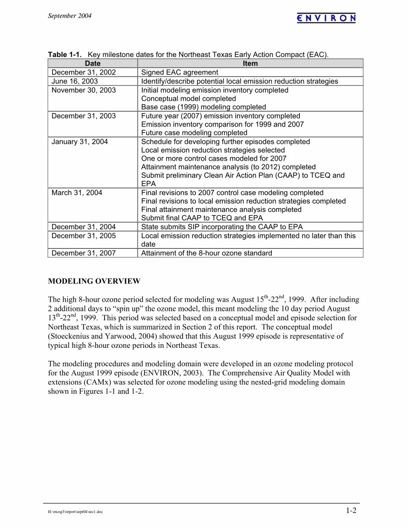
Table 1-1. Key milestone dates for the Northeast Texas Early Action Compact (EAC). Date Item
December 31, 2002 Signed EAC agreement June 16, 2003 Identify/describe potential local emission reduction strategies November 30, 2003 Initial modeling emission inventory completed
Conceptual model completed Base case (1999) modeling completed
December 31, 2003 Future year (2007) emission inventory completed Emission inventory comparison for 1999 and 2007 Future case modeling completed
January 31, 2004 Schedule for developing further episodes completed Local emission reduction strategies selected One or more control cases modeled for 2007 Attainment maintenance analysis (to 2012) completed Submit preliminary Clean Air Action Plan (CAAP) to TCEQ and EPA
March 31, 2004 Final revisions to 2007 control case modeling completed Final revisions to local emission reduction strategies completed Final attainment maintenance analysis completed Submit final CAAP to TCEQ and EPA
December 31, 2004 State submits SIP incorporating the CAAP to EPA December 31, 2005 Local emission reduction strategies implemented no later than this
date December 31, 2007 Attainment of the 8-hour ozone standard
MODELING OVERVIEW The high 8-hour ozone period selected for modeling was August 15th-22nd, 1999. After including 2 additional days to “spin up” the ozone model, this meant modeling the 10 day period August 13th-22nd, 1999. This period was selected based on a conceptual model and episode selection for Northeast Texas, which is summarized in Section 2 of this report. The conceptual model (Stoeckenius and Yarwood, 2004) showed that this August 1999 episode is representative of typical high 8-hour ozone periods in Northeast Texas. The modeling procedures and modeling domain were developed in an ozone modeling protocol for the August 1999 episode (ENVIRON, 2003). The Comprehensive Air Quality Model with extensions (CAMx) was selected for ozone modeling using the nested-grid modeling domain shown in Figures 1-1 and 1-2.

September 2004
H:\etcog3\report\sept04\sec1.doc 1-3
Figure 1-1. CAMx modeling domain for the August 1999 episode showing the 36-km regional grid and the nested 12-km and 4-km fine grids.

September 2004
H:\etcog3\report\sept04\sec1.doc 1-4
Figure 1-2. CAMx 4 km fine grid covering Northeast Texas for the August 1999 episode. OZONE LEVELS IN NORTHEAST TEXAS The TCEQ operates several continuous air monitoring stations (CAMS) in Northeast Texas as shown by the map in Figure 1-3. Historically, the highest ozone concentrations have been recorded at the Longview monitor (CAMS-19) located at the Gregg County airport where ozone data have been collected since the 1970s. Ozone monitoring commenced in 1995 at Tyler Airport (CAMS-86) although the monitor was relocated within the airport in 2000 due to construction and assigned a new number (CAMS-82). A monitoring site was established toward the east of the region at the Cypress River Airport (CAMS-50) in 1998. Cypress Riveris located to the north of Marshall in Marion County, which is not part of NETAC. The Cypress River monitor was discontinued in March 2001 and a new site located across the county line in Harrison County (Karnack, CAMS-85) began operating in September 2001. The CAMS 605 monitor was discontinued in October 2001 and the CAMS 133 monitor was discontinued in April 1991.

September 2004
H:\etcog3\report\sept04\sec1.doc 1-5
Figure 1-3. Location of Continuous Air Monitoring Stations (CAMS) operated by the TCEQ in Northeast Texas. CAMS 19, 82 and 50 were active in August 1999. Ozone trends for 1995 – 2002 at Longview and Tyler are compared with Dallas and Shreveport in Figure 1-4. This Figure shows annual 8-hour design values i.e., the 4th highest 8-hour ozone for the year. The data for Shreveport are based on the maximum of the Caddo and Bossier parish design values; annual 8-hour design values for Dallas are based on the maximum over five sites for which valid design values were available in each year. Trends at all locations share similar features. The annual design value in Dallas is higher than at the other locations in every year except 1998 and, in contrast to annual design values in Northeast Texas and Shreveport, did not drop off significantly in 2001 and 2002. Annual design values at Longview were comparable to those in Dallas during 1998 – 2000 but were much lower (and instead comparable to those at Tyler and in Shreveport) in 1996-1997 and 2001-2002. NETAC has undertaken research monitoring to collect ozone data at additional locations and supplemental precursor data at TCEQ monitoring locations. The NETAC research-monitoring site was located at Waskom in eastern Harrison County for the 2002 and 2003 ozone seasons and data were reported via the TCEQ’s data system as CAMS-612, which is shown in Figure 1-3.

September 2004
H:\etcog3\report\sept04\sec1.doc 1-6
Figure 1-4. Annual 8-hour ozone design values at locations in Northeast Texas, Dallas, and Shreveport, LA. The annual fourth highest daily maximum 8-hour ozone values for 2001 to 2003 are shown in Table 1-2 for monitors in Northeast Texas. The Karnack and Waskom monitors have only 2 years of data and so will not be used by EPA in attainment designations based on 2001 to 2003 data. Two-year design values are shown for Karnack and Waskom because they are used in the ozone attainment demonstration modeling (Section 6) and for comparison with Longview and Tyler. The preliminary 2001-2003 8-hour ozone design values for Longview and Tyler are both below 85 ppb and so Northeast Texas is monitoring attainment of the 8-hour standard. Table 1-2. Annual fourth highest daily maximum 8-hour ozone values and preliminary 2001-2003 8-hour ozone design values for Northeast Texas. Year Longview Tyler Karnack Waskom 2001 82 82 Partial Season Not Operating 2002 84 84 88 86 2003 82 79 80 82 Design Value 82 81 (84) (84)
Notes: The two-year design values for Karnack and Waskom are not used for attainment designation.
Annual 8-Hour Ozone Design ValueDallas, Longview, Tyler, and Shreveport
40
50
60
70
80
90
100
110
1995 1996 1997 1998 1999 2000 2001 2002
Year
ppb
Longview (1 site)Tyler (1 site)Dallas (5 sites)Shreveport (2 sites)
Data missing for October, 1996
September 2004
H:\etcog3\report\sept04\sec1.doc 1-7
REPORT ORGANIZATION Section 2 of this report describes the selection of the August 1999 modeling episode. The preparation of ozone model inputs is described in Sections 3 through 5 of this report. Section 3 describes the emission inventory development for the 1999 base year and 2002 and 2007 future years. Section 4 summarizes the meteorological modeling and extensive details are given in two supporting reports. Section 5 describes the preparation of other CAMx inputs. Section 6 describes the development of the 1999 base case including model evaluation procedures, diagnostic tests and sensitivity tests. The 1999 base case was refined through a series of improvements to the meteorology, emissions and CAMx inputs. The final 1999 base case was “base case7”. The 2007 base case was developed to evaluate future attainment of the ozone NAAQS. The final 2007 base case was “07base5.” The summary and conclusions at the end of Section 6 include recommendations for the next steps in EAC ozone modeling for Northeast Texas. Section 7 describes a detailed evaluation of which emissions sources were primarily responsible for high 8-hour ozone levels in Northeast Texas during the August 1999 episode. This analysis used the ozone source apportionment technology (OSAT) tools available on CAMx.

September 2004
H:\etcog3\report\sept04\sec2.doc 2-1
2. EPISODE SELECTION An episode selection analysis was performed to identify a period with representative high 8-hour ozone levels that was suitable for regional ozone modeling (ENVIRON, 2000). This analysis was reviewed and updated in developing a conceptual model for 8-hour ozone in Northeast Texas (Stoeckenius and Yarwood, 2004). The conceptual model concluded that the August 1999 episode selected for modeling remains a representative and appropriate choice. EPISODE SELECTION PROCEDURE Ozone data for Northeast Texas monitors from 1995 through 1999 were reviewed along with meteorological data such as back-trajectories and daily weather maps (ENVIRON, 2000). Episodes suitable for developing a new RSM for 8-hour ozone in Northeast Texas were identified by the following criteria: • Choose periods from the most recent three years at that time, i.e. 1997 to 1999. • Choose a multi-day period with 3 or more “high ozone” days as defined below. • Choose a period with high ozone at both Longview and Tyler. Based on the EPA draft
modeling guidance (EPA, 1999) and the 1997-1999 design values, high ozone was considered to be an 8-hour value of 85 - 101 ppb at Tyler, and 90 - 110 ppb at Longview.
• Choose a period with representative meteorological conditions for 8-hour ozone, which is
stagnation in Northeast Texas associated with a high regional ozone background and transport at the beginning of the stagnation period. This type of event is often referred to as a “regional haze event” because it is associated with hazy air across the whole East Texas region.
• Availability of supporting meteorological data, in particular data from the NCEP EDAS
model, is a strong advantage for modeling. EDAS data are available since 1997 with occasional missing days or blackout periods.
• Availability of special air-quality data, such as Baylor Aircraft flights and NETAC
monitoring studies, is an advantage. A search through 1997 to 1999 using these selection criteria listed above identified four candidate episodes:
1. August 26 to Sept 4, 1998 2. August 2 to August 7, 1999 3. August 15 to August 22, 1999 4. September 15 to September 20, 1999
The August/September 1998 period was given the lowest priority because important supporting meteorological data (the NCEP EDAS analyses) are missing for most of this period.

September 2004
H:\etcog3\report\sept04\sec2.doc 2-2
In selecting between the remaining two candidate periods, the August 1999 episode was given the highest priority for modeling because the September 1999 episode appears atypical and may be difficult to model for Northeast Texas. Specifically: • The meteorology during the September 1999 episode appears to be unusual for high ozone
episodes in Northeast Texas. – Temperatures were unusually cool for a Northeast Texas ozone episode. Maximum
temperatures at Longview were mostly in the mid 80’s rather than the high 90’s. – Upper level winds were from the west and unusually strong in the mid-troposphere
(about 5 km altitude). – Widespread daily rainfall occurred in North Texas and Oklahoma. Archived NEXRAD
data show rainfall in the area between Dallas to Shreveport on 4 of the 5 high ozone days. • An unusual ozone episode (such as September 1999) is not a good choice as the cornerstone
of 8-hour ozone control strategy development efforts. • Some of the unusual meteorological factors mentioned above are also likely to make this a
difficult period to model successfully for Northeast Texas. There is a greater risk of the September 1999 episode performing poorly in Northeast Texas than the August 1999 episode.
OZONE LEVELS FOR AUGUST 15-22, 1999 An August 15 – August 22, 1999 ozone episode was selected for evaluating 8-hour ozone in Northeast Texas (Stoeckenius et al., 2004). The modeling period was expanded to August 13 – August 22, 1999 to include 2 spin-up days before the start of the episode to reduce the influence in the modeling of initial conditions. As discussed below, this period includes combined influences from a high regional ozone background and local emissions, and includes a complete cycle of transport winds followed by local stagnation returning to transport winds at the end of the episode. This is a typical pattern for high 8-hour ozone events in Northeast Texas (Stoeckenius et al., 2004). The ozone data recorded at Continuous Air Monitoring Stations (CAMS) in Northeast Texas during this period are shown in Table 2-1. High ozone levels were recorded at all three CAMS during this period. On August 18th and 19th the ozone levels were similarly high at all three sites consistent with a high regional background of ozone. These high ozone levels built up between August 15th and 17th. This is consistent with the onset of meteorological stagnation on August 16th continuing through August 18th. Because the ozone-monitoring network in Northeast Texas is relatively sparse, the highest ozone levels on August 16th-18th may not have been recorded by a monitor. Ozone levels at Longview and Cypress River declined on August 20th and 21st, but then increased again on August 22nd. The pattern at Tyler is different on these days with higher ozone at Tyler on August 20th and 21st than on August 22nd.

September 2004
H:\etcog3\report\sept04\sec2.doc 2-3
Table 2-1. Maximum ozone levels and temperatures for the August 1999 episode days. Max 8-hour Ozone (ppb)
Date
Longview Maximum Temperature (ºF) Longview
CAMS 19 Tyler
CAMS 82 Cypress River
CAMS 50 8/15/99 93 66 73 55 8/16/99 95 105 92 71 8/17/99 96 110 97 90 8/18/99 99 88 74 91 8/19/99 102 91 85 81 8/20/99 97 80 86 70 8/21/99 95 87 92 67 8/22/99 96 91 77 82
Longview had especially high ozone monitored levels on August 16th and 17th that were significantly higher than at Tyler or Cypress River on these days consistent with a localized influence at Longview superimposed on the high regional background. There also are indications that Tyler experienced localized ozone impacts on August 15th, 20th and 21st because there were short periods when the ozone at Tyler spiked to higher levels than the other monitors. The localized impacts seen on some days at Longview and Tyler are consistent with plumes impacting the monitor locations. These plumes are likely to be associated with emissions sources within the Northeast Texas area and could be from either a major industrial source or an urban area. BACK TRAJECTORIES FOR AUGUST 15-22, 1999 Local wind data for Northeast Texas are available from the TCEQ CAMS, but while these data are useful for determining the wind direction in the immediate vicinity of a monitor, they are less useful for developing a conceptual picture of regional wind patterns during an ozone episode period. One way to evaluate the regional wind patterns is from back trajectories. The National Oceanic & Atmospheric Administration (NOAA) provides web-based tools to calculate back trajectories at http://www.arl.noaa.gov/ready/hysplit4.html. The NOAA back trajectories are based on archived data from weather forecasting models, so back trajectories are models rather than observations. A single back trajectory shows how a model predicts that air moved to arrive at a fixed end point in space and time. Back trajectories provide a simple picture of air movements to arrive at a given place and time. This picture should not be taken too literally since:
• Back trajectories are computer models with uncertainties. • The concept of a back trajectory over-simplifies the way air moves in the real atmosphere
by neglecting important effects such as vertical mixing and differences in wind speed/direction with height.
Back trajectories for days between August 16th and 22nd, 1999 are shown in Figure 2-1. These trajectories are based on archived wind data from the NOAA/NCEP Eta Data Analysis (EDAS)

September 2004
H:\etcog3\report\sept04\sec2.doc 2-4
system. The back trajectories end at the Longview CAMS-19 monitoring site at 15:00 hours CDT (which is 21:00 hours UTC in the trajectory labeling used in Figure 2-1). Back Trajectories were run for a duration of 32 hours, i.e., back to the morning of the day before, so that they indicate about 1.5 day transport distances. Back trajectories were run for ending altitudes of 500 m and 1000 m to provide an indication of whether wind shear was important. If the 500 m and 1000 m trajectories run in different directions, this indicates that there was significant variation in winds with altitude and that the back trajectory directions are highly uncertain. Back trajectories for August 16th through 22nd, 1999 are shown in Figure 2-1. These trajectories are based on archived wind data from the NOAA/NCEP Eta Data Analysis (EDAS) system. The back trajectories end at the Longview CAMS-19 monitoring site at 16:00 hours CDT (which is 21:00 hours UTC in the trajectory labeling used in Figure 2-1). Back Trajectories were run for a duration of 32 hours, i.e., back to the morning of the day before, so that they indicate about 1.5 day transport distances. Back trajectories were run for ending altitudes of 500 m and 1000 m to provide an indication of whether wind shear was important. If the 500 m and 1000 m trajectories run in different directions, this indicates that there was significant variation in winds with altitude and that the back trajectory directions are highly uncertain. The back trajectories show organized but weak easterly winds on August 16th transitioning to stagnation on August 17th. The stagnation persisted through August 19th. On August 20th the back trajectories become more organized again with winds from the northeast, but the back trajectories for August 20th (and August 21st) are unusual because the 500 m trajectories travel back further than the 1000 m trajectories. The back-trajectory for August 21st suggests that there was subsidence leading up to this day. On August 22nd the trajectories return to weak easterly winds and are similar to August 16th. This pattern shows a complete cycle of an episode beginning with transport winds from the East/Northeast followed by local stagnation returning to transport winds from the East/Northeast at the end of the episode. This is a typical pattern for high 8-hour ozone events in Northeast Texas (Stoeckenius et al., 2004).

September 2004
H:\etcog3\report\sept04\sec2.doc 2-5
August 16-19, 1999
Figure 2-1. Back trajectories from Longview (CAMS19) ending at 15:00 CDT.

September 2004
H:\etcog3\report\sept04\sec2.doc 2-6
August 20-22, 1999
Figure 2-1 (concluded). Back trajectories from Longview (CAMS19) ending at 15:00 CDT.
September 2004
H:\etcog3\report\sept04\sec2.doc 2-7
BACK TRAJECTORIES PLUS OBSERVED OZONE An analysis was carried out that combined back trajectories with observed ozone levels to investigate the potential for ozone transport. Figures were prepared that combined several types of data for a specific day:
• The daily maximum 1-hour ozone levels at the Longview, Tyler and Marshall CAMS. • The Longview back-trajectories ending at 15:00 and 500/1000 m. • The daily maximum 1-hour ozone for the previous day in surrounding areas (Louisiana,
Arkansas, Oklahoma). Previous day ozone levels are shown for the surrounding areas because the back trajectories are 1.5 days long from end (Longview) to start.
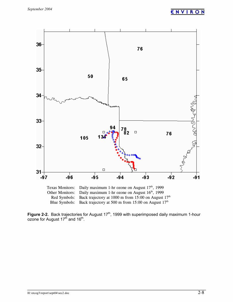
Figures 2-2 through 2-4 show these analyses for August 17th, 20th and 22nd, respectively. Limitations to keep in mind are that the back-trajectories only provide an indication of the likely transport direction and distance, and that the upwind monitored values may not represent regional ozone levels because many of them are in urban areas. On August 17th (Figure 2-2), the back trajectories are short and meandering consistent with stagnation. Air in Northeast Texas may have been in Northwest Louisiana on the previous day Peak ozone levels in Northeast Texas on August 17th (94 ppb to 134 ppb) were much higher than in Northwest Louisiana on August 16th (78 ppb to 82 ppb), suggesting a significant contribution from local emissions to the high ozone levels in Northeast Texas on August 17th, 1999. For August 20th (Figure 2-3), the back trajectories suggest that the air in Northeast Texas may have come from an area between Northern Louisiana to Western Arkansas on the previous day. Peak ozone levels in Northeast Texas on August 20th (72 ppb to 99 ppb) were similar to the levels in this upwind area on August 19th (84 ppb to 97 ppb) suggesting that the high ozone in Northeast Texas on August 20th was part of a regional high ozone event that was transported through the region. For August 22nd (Figure 2-4), the back trajectories suggest that the air in Northeast Texas may have come from Northwest Louisiana on the previous day. Peak ozone levels in Northeast Texas on August 22nd (78 ppb to 107 ppb) were higher than the levels in Northwest Louisiana on August 21st (68 ppb to 73 ppb) suggesting a moderate contribution from local emissions to the high ozone levels in Northeast Texas on August 22nd, 1999.
September 2004
H:\etcog3\report\sept04\sec2.doc 2-8
Texas Monitors: Other Monitors:
Red Symbols: Blue Symbols:
Daily maximum 1-hr ozone on August 17th, 1999 Daily maximum 1-hr ozone on August 16th, 1999 Back trajectory at 1000 m from 15:00 on August 17th Back trajectory at 500 m from 15:00 on August 17th
Figure 2-2. Back trajectories for August 17th, 1999 with superimposed daily maximum 1-hour ozone for August 17th and 16th.

September 2004
H:\etcog3\report\sept04\sec2.doc 2-9
Texas Monitors: Other Monitors:
Red Symbols: Blue Symbols:
Daily maximum 1-hr ozone on August 20th, 1999 Daily maximum 1-hr ozone on August 19th, 1999 Back trajectory at 1000 m from 15:00 on August 20th Back trajectory at 500 m from 15:00 on August 20th
Figure 2-3. Back trajectories for August 20th, 1999 with superimposed daily maximum 1-hour ozone for August 20th and 19th.

September 2004
H:\etcog3\report\sept04\sec2.doc 2-10
Texas Monitors: Other Monitors:
Red Symbols: Blue Symbols:
Daily maximum 1-hr ozone on August 22nd, 1999 Daily maximum 1-hr ozone on August 21st, 1999 Back trajectory at 1000 m from 15:00 on August 22nd Back trajectory at 500 m from 15:00 on August 22nd
Figure 2-4. Back trajectories for August 22nd, 1999 with superimposed daily maximum 1-hour ozone for August 22nd and 21st.

September 2004
H:\etcog3\report\sept04\sec3.doc 3-1
3. EMISSIONS MODELING This section describes the emission inventory preparation for the August 13-22, 1999 modeling episode for the East Texas Near Non-Attainment Area (NNA). Emission inventories are processed using version 2x of the Emissions Processing System (EPS2x) for area, off-road, onroad mobile and point sources. The purpose of the emissions processing is to format the emission inventory for CAMx photochemical modeling. Specifically, the emission inventory is allocated: • Temporally – to account for seasonal, day of weak and hour of day variability • Spatially – to reflect the geographic distributions of emissions • Chemically – to account for the chemical composition of VOC and NOx emissions in terms
of the Carbon Bond 4 (CB4) chemical mechanism used in CAMx. Emissions for different major source groups (e.g., mobile, non-road mobile, area, point and biogenic) are processed separately and merged together prior to CAMx modeling. This simplifies the processing and assists quality assurance (QA) and reporting tasks. The biogenic inventories are generated with GloBEIS version 3.1. The August 13-22,1999 episode, a Friday through Sunday, is being modeled in CAMx using a Lambert Conformal Projection (LCP) nested grid configuration with grid resolutions of 36, 12 and 4 km (Figure 1-1). In CAMx, emissions are separated between surface (surface and low level point) emissions and elevated point source emissions. For the surface emissions, a separate emission inventory is required for each grid nest, i.e., three inventories. For elevated point sources, a single emission inventory is prepared covering all grid nests. Two emissions modeling domains are used to generate the required CAMx ready inventories: 1. Near Non-Attainment Area 4 km Grid. The NNA emissions grid has 54 x 45 cells at 4 km
resolution and covers the same area as the CAMx 4 km nested grid shown in Figures 1-1 and 1-2.
2. Regional Emissions Grid. The regional emissions grid has 135 x 138 cells at 12-km
resolution and covers the full area shown in Figure 1-1. This emissions grid is used for the 12 km CAMx grid by “windowing out” emissions for the appropriate region. In addition the regional emissions grid is aggregated from three by three 12-km cells to one 36-km cell over the entire area to generate the CAMx 36km grid.
Emission inventories were prepared for the 1999 base year and for 2002 and 2007 future years. The emissions data sources and processing are described separately below for point, onroad mobile, area, off-road, and biogenic sources. Following the data descriptions are summary tables.

September 2004
H:\etcog3\report\sept04\sec3.doc 3-2
DATA SOURCES FOR 1999 Point Sources Point source data were obtained from several different sources, processed separately and merged prior to modeling. The data include: • Texas electric generating units (EGUs) • Texas non-EGU point sources • Facility specific data • Texas minor point sources • Louisiana EGUs • Louisiana non-EGUs
• Oklahoma EGUs • Oklahoma non-EGUs • Other State point sources The point source data are processed for a typical peak ozone (PO) season weekday and weekend day. The exception is Texas, Louisiana and Oklahoma EGUs, which are hourly episode day specific data, based on continuous emissions monitor (CEM) data that were reported to EPA’s “Acid Rain” database. The 1999 Texas and Louisiana point source data were provided by TCEQ in EPS2 AFS input format. The TCEQ Point Source Data Base (PSDB) version 15a for 1999 is the basis of the non-EGU Texas data. Day specific data was provided for two stacks at the Eastman Chemical Company facility via email from J. Woolbert (NOXFOROZ-aug99.xls). The other emissions for Texas Eastman Chemical Company were provided by NETAC. Louisiana Department of Environmental Quality (LDEQ) provided TCEQ with a copy of their point source inventory which TCEQ converted into AFS format. The files that were downloaded from the TCEQ ftp site ftp://ftp.TCEQ.state.tx.us/pub/AirQuality/AirQualityPlanningAssessment/Modeling/ are:
TX EGU DFWAQSE/Modeling/EI/Points/1999/hourly_TXegu_990813-990822.v15a.lcp.3pols
TX Non-EGU DFWAQSE/Modeling/EI/Points/1999/afs.tx_negu.990813-990822.v15a.lcp.3pols
TX Minor Points file-transfer/NearNon/afs.0813-2299minorpts_nna LA EGU file-transfer/NearNon/hourly_LAegu_0813-2299.afs_v4_latlon LA Non-EGU file-transfer/NearNon/afs.LA_0813-2299v4_latlon_negu
The Oklahoma EGU data were downloaded from the Acid Rain database. In addition, the 1999 NEI v2 Oklahoma data were reviewed and corrected by ODEQ before processing. For all states other than Texas, Louisiana and Oklahoma the National Emission Inventory (NEI) 1999 Version 2 for Criteria Pollutants data is used. The Access database files SS99CritPt1002.mdb (where SS is the state abbreviation) were downloaded from EPA’s ftp site. The data is processed to (1) relate separate data tables by common fields, (2) query to extract peak ozone season data for those states within the regional modeling domain and (3) export the

September 2004
H:\etcog3\report\sept04\sec3.doc 3-3
resultant data table to an ASCII text file for processing through EPS2x. The criteria for selecting NOx point sources for plume in grid treatment within the 4-km modeling domain is 2 tons NOx on any episode day. For the regional emissions grid, the NOx criteria is 25 tons per day on any episode day. Mobile Sources The Texas Transportation Institute (TTI) prepared mobile source emissions for all Texas counties under contract to the TCEQ. Emission factors are from the EPA’s MOBILE6 model. Vehicle miles traveled (VMT) for 1999 are based on transportation models in all NNA counties that have a complete transportation model and were based on a rural HPMS method elsewhere. The NNA counties for which link based transportation model data are used:
East Texas: Gregg, Smith Austin: Hays, Travis, Williamson San Antonio: Bexar Corpus Christi: Nueces, San Patricio Victoria: Victoria
TTI calculated emissions for each hour for four day-of-week scenarios: Monday-Thursday, Friday, Saturday and Sunday. The temperatures and humidities are for average August/September 1999 conditions in each county. The emissions are adjusted from the average scenario to day specific temperature and humidities in each county for modeling. The emissions reported here are for the average temperature/humidity scenario used by TTI. Table 3-1. 1999 Texas onroad mobile source emissions (tons per day) from TTI for typical July/August 1999 conditions.
Weekday Friday Saturday Sunday County NOx VOC CO NOx VOC CO NOx VOC CO NOx VOC CO Bexar 122 82 935 114 80 913 70 51 640 50 41 528Gregg 26 6 78 25 8 97 18 7 88 13 6 86Hays 11 5 70 10 5 75 7 4 59 5 3 53Nueces 21 15 198 21 19 234 16 14 182 12 11 156San Patricio 5 4 45 5 4 53 4 3 41 3 3 35Smith 28 10 130 29 13 158 21 11 146 16 10 140Travis 63 33 409 58 35 436 39 25 341 30 22 303Victoria 9 4 51 10 5 69 7 4 56 6 5 61Williamson 17 9 118 16 10 126 11 7 98 8 6 87All Others 1103 669 8676 786 581 7404 548 433 5803 426 379 5135Total 1404 836 10712 1074 759 9565 740 559 7453 570 487 65811 Named counties have link-based data. All others have HPMS format activity data. The emissions estimates prepared by TTI reflect a temperature/humidity profile for an average August/September day. To adjust for episodic conditions, a methodology was developed to calculate a temperature/humidity adjustment factor for each county. The steps in the process are as follows:
1. Run the MOBILE6 model using the county-level temperature/humidity profile used by TTI and extract the emission factors.

September 2004
H:\etcog3\report\sept04\sec3.doc 3-4
2. For each day in the modeling episode, run the MOBILE6 model using the county-
level episodic conditions and extract the emission factors. 3. Calculate the ratio of episodic emission factor to base emission factor and apply this
ratio to the emissions estimate generated by TTI. The result of this processing was a mobile emissions inventory that accurately reflects the temperature and humidity in a given county during the modeling period. The link-based emissions are then speciated into CAMx chemical species and written to a CAMx emissions file using EPS2x. The inventory in counties with only county-wide VMT estimates required a gridding step, which was also implemented with EPS2x modules using gridded spatial surrogates. County specific HPMS VMT and speed data for Oklahoma were provided by the Oklahoma Department of Transportation. Mobile6.2 emission factors were used to calculate county-level mobile emissions estimates for Oklahoma. The emissions estimates were processed through the EPS2x system to generate episode specific model-ready emissions estimates. The NEI 1999 Version 2 for Criteria Pollutants, released by EPA October 2002, is the basis for the onroad mobile regional emissions inventory for those counties outside Texas and Oklahoma. The data file 99neiv2asciionroad.zip - 1999 NEI Version 2 Criteria Emissions from Onroad Mobile Sources in ASCII text format was acquired from EPA’s ftp site (ftp://ftp.epa.gov). The NEI 1999 onroad emission inventory is processed to (1) extract the typical peak ozone season day data, (2) reformatted to the EPS2x AMS input file format and (3) processed through EPS2x. A rural and urban road type spatial distribution is used to spatially allocate the urban and rural onroad sources. Area Sources Area emissions estimates for the counties within the East Texas NNA were based on the NETAC 1999 inventory. Refer to “Tyler/Longview/Marshall Flexible Attainment Region Emission Inventory Ozone Prescursors, VOC, NOx and CO 1999 Emissions” May 2002 for a detailed description of the inventory development. Jerry Demo of Pollution Solutions provided these data via email. The TCEQ provided emission inventories for Texas area sources. The data were downloaded from the TCEQ domain at /pub/AirQuality/AirQualityPlanningAssessment/Modeling/file_transfer/TX99AreaNR. The file ams. TX_99.area_base1 are in EPS2x input file format. For all areas outside Texas, the NEI 1999 Version 2 for Criteria Pollutants, released by EPA November 2002, is the basis for the area regional emissions inventory. The data file 99neiv2asciiarea.zip - 1999 NEI Version 2 Criteria Emissions from Area Sources in ASCII text format was acquired from EPA’s ftp site. The file format documentation is provided at http://www.epa.gov/ttn/chief/eidocs/index.html#pack. The NEI 1999 area emission inventory is (1) processed to extract the typical peak ozone season day data, (2) reformatted to the EPS2x

September 2004
H:\etcog3\report\sept04\sec3.doc 3-5
AMS input file format and (3) processed through EPS2x. Off-Road Sources Off-road source emissions were estimated with NonRoadv2002 using local survey data for mining and construction equipment for the counties within the East Texas NNA. The aircraft and railroad emissions were based on the NETAC 1999 inventory. Refer to “Tyler/Longview/Marshall Flexible Attainment Region Emission Inventory Ozone Prescursors, VOC, NOx and CO 1999 Emissions” May 2002 for a detailed description of the inventory development. Jerry Demo of Pollution Solutions provided these data via email. The other Texas county off-road emissions were estimated with NonRoadv2002. The aircraft, commercial marine and railroad emissions were extracted from the TCEQ emission inventory for Texas off-road sources. The data were downloaded from the TCEQ domain at /pub/AirQuality/AirQualityPlanningAssessment/Modeling/file_transfer/TX99AreaNR. The files ams.TX_99.NR_base1 are in EPS2x input file format. For all areas outside Texas the NEI 1999 Version 2 for Criteria Pollutants, released by EPA October 2002, is the basis for the off-road regional emissions inventory. The data file 99neiv2asciinonroad.zip - 1999 NEI Version 2 Criteria Emissions from Nonroad Sources in ASCII text format was acquired from EPA’s ftp site (ftp://ftp.epa.gov) and based on the NonRoadv2002 Model. The NEI 1999 off-road emission inventory is (1) processed to extract the typical peak ozone season day data, (2) reformatted to the EPS2x AMS input file format and (3) processed through EPS2x. The ODEQ provided corrections and updates for the state of Oklahoma NEI inventory. Biogenic Sources Biogenic emissions were prepared using version 3.1 of the GloBEIS model (Yarwood et al., 2002). The GloBEIS model was developed by the National Center for Atmospheric Research and ENVIRON under sponsorship from the TCEQ. GloBEIS3.1 is based on the EPA BEIS2 model with the following improvements: • Updated emission factor algorithm (called the BEIS99 algorithm). • Compatible with the EPA’s BELD3 landuse/landcover (LULC) database. • Compatible with the TCEQ’s Texas specific LULC database (Yarwood et al., 2001) which
includes local survey data for Northeast Texas developed by NETAC (ENVIRON, 1999). • Ability to use solar radiation data for photosynthetically active radiation (PAR). • Takes into account the effects of drought stress and prolonged periods of high temperature. The preparation of biogenic emission inventories is described in detail at the end of Section 3. EMISSIONS SUMMARIES FOR 1999 All emission estimates in the following tables reflect gridded, model ready emissions. This means that for partial counties and/or states at the edge of a modeling domain, only the portion
September 2004
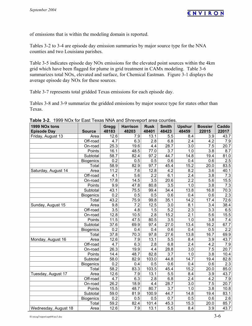
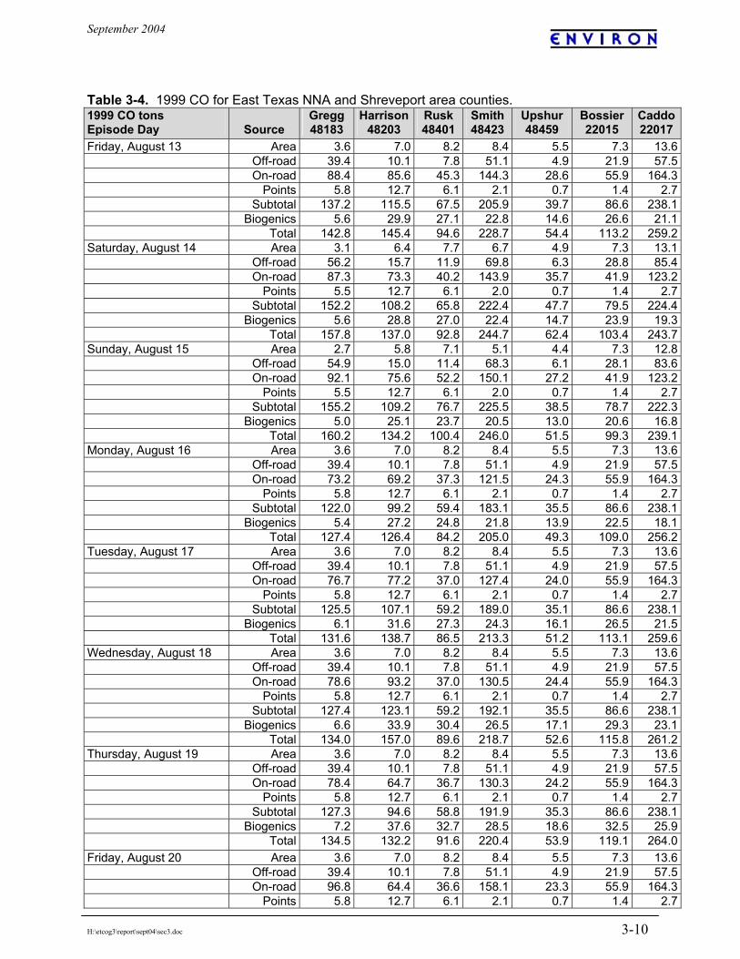
H:\etcog3\report\sept04\sec3.doc 3-6
of emissions that is within the modeling domain is reported. Tables 3-2 to 3-4 are episode day emission summaries by major source type for the NNA counties and two Louisiana parishes. Table 3-5 indicates episode day NOx emissions for the elevated point sources within the 4km grid which have been flagged for plume in grid treatment in CAMx modeling. Table 3-6 summarizes total NOx, elevated and surface, for Chemical Eastman. Figure 3-1 displays the average episode day NOx for these sources. Table 3-7 represents total gridded Texas emissions for each episode day. Tables 3-8 and 3-9 summarize the gridded emissions by major source type for states other than Texas. Table 3-2. 1999 NOx for East Texas NNA and Shreveport area counties. 1999 NOx tons Episode Day Source
Gregg 48183
Harrison 48203
Rusk 48401
Smith 48423
Upshur 48459
Bossier 22015
Caddo22017
Friday, August 13 Area 12.6 7.9 13.1 5.5 8.4 3.9 43.7 Off-road 4.7 6.3 2.8 6.8 2.4 4.2 7.9 On-road 25.3 19.6 4.4 28.7 3.0 7.5 20.7 Points 16.1 48.5 77.0 3.7 1.0 3.8 8.7 Subtotal 58.7 82.4 97.2 44.7 14.8 19.4 81.0 Biogenics 0.2 0.5 0.5 0.6 0.4 0.6 2.5 Total 58.9 82.9 97.7 45.4 15.2 20.0 83.5Saturday, August 14 Area 11.2 7.6 12.8 4.2 8.2 3.6 40.1 Off-road 4.1 5.6 2.2 6.1 2.4 3.8 7.3 On-road 17.8 14.5 3.5 20.6 2.2 5.6 15.5 Points 9.9 47.8 80.8 3.5 1.0 3.8 7.3 Subtotal 43.1 75.5 99.4 34.4 13.8 16.8 70.3 Biogenics 0.2 0.5 0.5 0.6 0.4 0.6 2.3 Total 43.2 75.9 99.8 35.1 14.2 17.4 72.6Sunday, August 15 Area 9.8 7.2 12.5 3.0 8.1 3.4 38.4 Off-road 3.5 4.8 1.5 5.2 2.3 3.3 6.5 On-road 12.8 10.5 2.8 15.2 2.1 5.6 15.5 Points 11.5 47.5 80.5 3.5 1.0 3.8 7.4 Subtotal 37.6 69.9 97.4 27.0 13.4 16.2 67.7 Biogenics 0.2 0.4 0.4 0.6 0.4 0.5 2.2 Total 37.8 70.3 97.8 27.6 13.8 16.7 69.9Monday, August 16 Area 12.6 7.9 13.1 5.5 8.4 3.9 43.7 Off-road 4.7 6.3 2.8 6.8 2.4 4.2 7.9 On-road 26.3 19.9 4.4 28.8 3.0 7.5 20.7 Points 14.4 48.7 82.8 3.7 1.0 3.8 10.4 Subtotal 58.0 82.9 103.0 44.8 14.7 19.4 82.8 Biogenics 0.2 0.4 0.5 0.6 0.4 0.6 2.3 Total 58.2 83.3 103.5 45.4 15.2 20.0 85.0Tuesday, August 17 Area 12.6 7.9 13.1 5.5 8.4 3.9 43.7 Off-road 4.7 6.3 2.8 6.8 2.4 4.2 7.9 On-road 26.2 18.9 4.4 28.7 3.0 7.5 20.7 Points 15.5 48.7 80.7 3.7 1.0 3.8 10.8 Subtotal 59.0 81.9 100.9 44.7 14.8 19.4 83.1 Biogenics 0.2 0.5 0.5 0.7 0.5 0.6 2.6 Total 59.2 82.4 101.4 45.3 15.3 20.0 85.7Wednesday, August 18 Area 12.6 7.9 13.1 5.5 8.4 3.9 43.7

September 2004
H:\etcog3\report\sept04\sec3.doc 3-7
1999 NOx tons Episode Day Source
Gregg 48183
Harrison 48203
Rusk 48401
Smith 48423
Upshur 48459
Bossier 22015
Caddo22017
Off-road 4.7 6.3 2.8 6.8 2.4 4.2 7.9 On-road 25.5 20.2 4.4 27.9 3.0 7.5 20.7 Points 14.8 45.9 76.2 3.7 1.0 3.8 10.9 Subtotal 57.5 80.4 96.5 43.9 14.8 19.4 83.2 Biogenics 0.2 0.5 0.5 0.7 0.5 0.7 2.7 Total 57.7 80.9 97.0 44.6 15.3 20.1 85.9Thursday, August 19 Area 12.6 7.9 13.1 5.5 8.4 3.9 43.7 Off-road 4.7 6.3 2.8 6.8 2.4 4.2 7.9 On-road 25.6 20.2 4.4 28.0 2.9 7.5 20.7 Points 16.1 49.9 77.2 3.7 1.0 3.8 11.2 Subtotal 59.0 84.3 97.4 44.0 14.7 19.4 83.5 Biogenics 0.2 0.6 0.6 0.8 0.5 0.7 3.0 Total 59.2 84.9 98.0 44.7 15.2 20.1 86.5Friday, August 20 Area 12.6 7.9 13.1 5.5 8.4 3.9 43.7 Off-road 4.7 6.3 2.8 6.8 2.4 4.2 7.9 On-road 25.1 20.1 4.4 28.5 3.1 7.5 20.7 Points 17.6 45.6 81.8 3.7 1.0 3.8 11.8 Subtotal 60.0 80.0 102.1 44.5 14.8 19.4 84.1 Biogenics 0.2 0.5 0.5 0.6 0.4 0.6 2.5 Total 60.2 80.4 102.6 45.2 15.3 20.0 86.6Saturday, August 21 Area 11.2 7.6 12.8 4.2 8.2 3.6 40.1 Off-road 4.1 5.6 2.2 6.1 2.4 3.8 7.3 On-road 18.3 14.6 3.6 21.1 2.4 5.6 15.5 Points 16.2 22.1 80.6 3.5 1.0 3.8 12.0 Subtotal 49.9 49.9 99.3 35.0 14.0 16.8 75.0 Biogenics 0.2 0.5 0.5 0.6 0.4 0.6 2.4 Total 50.1 50.4 99.8 35.7 14.4 17.4 77.4Sunday, August 22 Area 9.8 7.2 12.5 3.0 8.1 3.4 38.4 Off-road 3.5 4.8 1.5 5.2 2.3 3.3 6.5 On-road 13.5 10.2 2.9 16.1 2.0 5.6 15.5 Points 12.6 38.9 84.1 3.5 1.0 3.8 9.6 Subtotal 39.4 61.0 101.1 27.8 13.3 16.2 70.0 Biogenics 0.2 0.5 0.5 0.7 0.4 0.6 2.5 Total 39.6 61.5 101.6 28.5 13.8 16.8 72.5Average Episode Day Area 12.0 7.8 12.9 5.0 8.3 3.8 42.4 Off-road 4.4 6.0 2.5 6.5 2.4 4.0 7.6 On-road 22.9 17.7 4.1 25.5 2.7 6.9 19.2 Points 14.7 45.5 79.9 3.6 1.0 3.8 10.2 Subtotal 54.0 77.0 99.4 40.6 14.4 18.6 79.5 Biogenics 0.2 0.5 0.5 0.7 0.4 0.6 2.5 Total 54.2 77.5 99.9 41.3 14.9 19.2 82.1

September 2004
H:\etcog3\report\sept04\sec3.doc 3-8
Table 3-3. 1999 VOC for East Texas NNA and Shreveport area counties. 1999 VOC tons Episode Day Source
Gregg 48183
Harrison 48203
Rusk 48401
Smith 48423
Upshur 48459
Bossier 22015
Caddo22017
Friday, August 13 Area 14.8 13.4 11.9 14.6 13.5 6.2 26.4 Off-road 2.4 1.2 0.8 3.8 0.4 1.7 4.5 On-road 6.7 6.4 3.7 10.9 2.3 5.4 16.1 Points 3.5 15.6 2.0 8.9 0.8 1.6 5.8 Subtotal 27.4 36.6 18.5 38.2 17.0 14.9 52.7 Biogenics 64.2 325.9 280.4 254.5 154.0 298.7 238.5 Total 91.6 362.5 298.9 292.6 170.9 313.5 291.3Saturday, August 14 Area 11.5 11.3 10.1 10.1 12.5 6.2 26.3 Off-road 2.9 2.2 1.7 5.4 0.7 2.6 7.4 On-road 6.4 5.1 3.2 10.5 2.9 4.1 12.1 Points 3.1 14.6 2.0 7.7 0.8 1.6 5.8 Subtotal 23.9 33.3 16.9 33.6 16.9 14.5 51.6 Biogenics 61.2 297.1 263.2 234.8 148.9 259.0 205.0 Total 85.1 330.4 280.1 268.4 165.7 273.5 256.6Sunday, August 15 Area 10.0 10.4 9.3 7.7 11.9 6.2 26.3 Off-road 2.8 2.1 1.6 5.2 0.7 2.5 7.2 On-road 6.8 5.3 4.3 11.0 2.1 4.1 12.1 Points 3.1 14.6 2.0 7.7 0.8 1.6 5.8 Subtotal 22.6 32.4 17.1 31.6 15.5 14.4 51.4 Biogenics 54.5 257.5 231.2 218.1 132.0 218.3 176.4 Total 77.1 289.9 248.4 249.7 147.5 232.7 227.8Monday, August 16 Area 14.8 13.4 11.9 14.6 13.5 6.2 26.4 Off-road 2.4 1.2 0.8 3.8 0.4 1.7 4.5 On-road 5.8 5.2 3.1 9.5 2.0 5.4 16.1 Points 3.5 15.6 2.0 8.9 0.8 1.6 5.8 Subtotal 26.5 35.3 17.9 36.8 16.7 14.9 52.7 Biogenics 57.9 276.2 240.2 228.2 140.2 236.6 185.4 Total 84.4 311.5 258.1 265.0 156.9 251.5 238.2Tuesday, August 17 Area 14.8 13.4 11.9 14.6 13.5 6.2 26.4 Off-road 2.4 1.2 0.8 3.8 0.4 1.7 4.5 On-road 6.3 7.2 3.1 10.2 2.0 5.4 16.1 Points 3.5 15.6 2.0 8.9 0.8 1.6 5.8 Subtotal 27.0 37.3 17.8 37.5 16.7 14.9 52.7 Biogenics 64.8 322.8 264.4 250.1 160.9 285.1 225.4 Total 91.8 360.1 282.2 287.6 177.6 299.9 278.1Wednesday, August 18 Area 14.8 13.4 11.9 14.6 13.5 6.2 26.4 Off-road 2.4 1.2 0.8 3.8 0.4 1.7 4.5 On-road 6.4 4.7 3.0 10.4 2.0 5.4 16.1 Points 3.5 15.6 2.0 8.9 0.8 1.6 5.8 Subtotal 27.1 34.9 17.7 37.7 16.7 14.9 52.7 Biogenics 70.0 343.6 292.5 273.6 168.8 312.2 242.7 Total 97.1 378.5 310.3 311.2 185.4 327.0 295.5Thursday, August 19 Area 14.8 13.4 11.9 14.6 13.5 6.2 26.4 Off-road 2.4 1.2 0.8 3.8 0.4 1.7 4.5 On-road 6.3 4.7 3.0 10.3 1.8 5.4 16.1 Points 3.5 15.6 2.0 8.9 0.8 1.6 5.8 Subtotal 27.0 34.8 17.8 37.5 16.5 14.9 52.7 Biogenics 76.7 377.5 316.4 299.0 184.4 339.1 267.8
Total 103.7 412.3 334.2 336.5 200.9 354.0 320.5Friday, August 20 Area 14.8 13.4 11.9 14.6 13.5 6.2 26.4 Off-road 2.4 1.2 0.8 3.8 0.4 1.7 4.5 On-road 7.7 5.8 3.4 12.6 2.4 5.4 16.1 Points 3.5 15.6 2.0 8.9 0.8 1.6 5.8

September 2004
H:\etcog3\report\sept04\sec3.doc 3-9
1999 VOC tons Episode Day Source
Gregg 48183
Harrison 48203
Rusk 48401
Smith 48423
Upshur 48459
Bossier 22015
Caddo22017
Subtotal 28.4 36.0 18.1 39.8 17.1 14.9 52.7 Biogenics 65.4 313.7 281.7 254.1 152.4 274.5 220.0 Total 93.8 349.6 299.8 293.9 169.5 289.3 272.7Saturday, August 21 Area 11.5 11.3 10.1 10.1 12.5 6.2 26.3 Off-road 2.9 2.2 1.7 5.4 0.7 2.6 7.4 On-road 6.7 5.0 3.1 10.9 1.9 4.1 12.1 Points 3.1 14.6 2.0 7.7 0.8 1.6 5.8 Subtotal 24.2 33.2 16.8 34.1 15.9 14.5 51.6 Biogenics 61.8 292.0 258.1 242.2 148.3 253.4 202.4 Total 86.0 325.1 274.9 276.3 164.2 267.9 254.0Sunday, August 22 Area 10.0 10.4 9.3 7.7 11.9 6.2 26.3 Off-road 2.8 2.1 1.6 5.2 0.7 2.5 7.2 On-road 6.4 5.4 2.9 10.3 1.8 4.1 12.1 Points 3.1 14.6 2.0 7.7 0.8 1.6 5.8 Subtotal 22.2 32.5 15.7 31.0 15.2 14.4 51.4 Biogenics 64.2 308.5 263.8 249.2 155.1 263.5 210.7 Total 86.4 341.0 279.5 280.1 170.2 277.9 262.1Average Episode Day Area 13.6 12.7 11.3 13.0 13.1 6.2 26.4 Off-road 2.5 1.5 1.1 4.2 0.5 1.9 5.3 On-road 6.5 5.5 3.2 10.5 2.1 5.0 14.9 Points 3.4 15.3 2.0 8.5 0.8 1.6 5.8 Subtotal 26.0 34.9 17.5 36.2 16.5 14.7 52.4 Biogenics 65.0 316.8 271.8 253.9 157.1 279.5 221.1 Total 91.0 351.7 289.4 290.1 173.5 294.3 273.5
September 2004
H:\etcog3\report\sept04\sec3.doc 3-10
Table 3-4. 1999 CO for East Texas NNA and Shreveport area counties. 1999 CO tons Episode Day
Source
Gregg 48183
Harrison48203
Rusk 48401
Smith 48423
Upshur 48459
Bossier 22015
Caddo22017
Friday, August 13 Area 3.6 7.0 8.2 8.4 5.5 7.3 13.6 Off-road 39.4 10.1 7.8 51.1 4.9 21.9 57.5 On-road 88.4 85.6 45.3 144.3 28.6 55.9 164.3 Points 5.8 12.7 6.1 2.1 0.7 1.4 2.7 Subtotal 137.2 115.5 67.5 205.9 39.7 86.6 238.1 Biogenics 5.6 29.9 27.1 22.8 14.6 26.6 21.1 Total 142.8 145.4 94.6 228.7 54.4 113.2 259.2Saturday, August 14 Area 3.1 6.4 7.7 6.7 4.9 7.3 13.1 Off-road 56.2 15.7 11.9 69.8 6.3 28.8 85.4 On-road 87.3 73.3 40.2 143.9 35.7 41.9 123.2 Points 5.5 12.7 6.1 2.0 0.7 1.4 2.7 Subtotal 152.2 108.2 65.8 222.4 47.7 79.5 224.4 Biogenics 5.6 28.8 27.0 22.4 14.7 23.9 19.3 Total 157.8 137.0 92.8 244.7 62.4 103.4 243.7Sunday, August 15 Area 2.7 5.8 7.1 5.1 4.4 7.3 12.8 Off-road 54.9 15.0 11.4 68.3 6.1 28.1 83.6 On-road 92.1 75.6 52.2 150.1 27.2 41.9 123.2 Points 5.5 12.7 6.1 2.0 0.7 1.4 2.7 Subtotal 155.2 109.2 76.7 225.5 38.5 78.7 222.3 Biogenics 5.0 25.1 23.7 20.5 13.0 20.6 16.8 Total 160.2 134.2 100.4 246.0 51.5 99.3 239.1Monday, August 16 Area 3.6 7.0 8.2 8.4 5.5 7.3 13.6 Off-road 39.4 10.1 7.8 51.1 4.9 21.9 57.5 On-road 73.2 69.2 37.3 121.5 24.3 55.9 164.3 Points 5.8 12.7 6.1 2.1 0.7 1.4 2.7 Subtotal 122.0 99.2 59.4 183.1 35.5 86.6 238.1 Biogenics 5.4 27.2 24.8 21.8 13.9 22.5 18.1 Total 127.4 126.4 84.2 205.0 49.3 109.0 256.2Tuesday, August 17 Area 3.6 7.0 8.2 8.4 5.5 7.3 13.6 Off-road 39.4 10.1 7.8 51.1 4.9 21.9 57.5 On-road 76.7 77.2 37.0 127.4 24.0 55.9 164.3 Points 5.8 12.7 6.1 2.1 0.7 1.4 2.7 Subtotal 125.5 107.1 59.2 189.0 35.1 86.6 238.1 Biogenics 6.1 31.6 27.3 24.3 16.1 26.5 21.5 Total 131.6 138.7 86.5 213.3 51.2 113.1 259.6Wednesday, August 18 Area 3.6 7.0 8.2 8.4 5.5 7.3 13.6 Off-road 39.4 10.1 7.8 51.1 4.9 21.9 57.5 On-road 78.6 93.2 37.0 130.5 24.4 55.9 164.3 Points 5.8 12.7 6.1 2.1 0.7 1.4 2.7 Subtotal 127.4 123.1 59.2 192.1 35.5 86.6 238.1 Biogenics 6.6 33.9 30.4 26.5 17.1 29.3 23.1 Total 134.0 157.0 89.6 218.7 52.6 115.8 261.2Thursday, August 19 Area 3.6 7.0 8.2 8.4 5.5 7.3 13.6 Off-road 39.4 10.1 7.8 51.1 4.9 21.9 57.5 On-road 78.4 64.7 36.7 130.3 24.2 55.9 164.3 Points 5.8 12.7 6.1 2.1 0.7 1.4 2.7 Subtotal 127.3 94.6 58.8 191.9 35.3 86.6 238.1 Biogenics 7.2 37.6 32.7 28.5 18.6 32.5 25.9 Total 134.5 132.2 91.6 220.4 53.9 119.1 264.0Friday, August 20 Area 3.6 7.0 8.2 8.4 5.5 7.3 13.6 Off-road 39.4 10.1 7.8 51.1 4.9 21.9 57.5 On-road 96.8 64.4 36.6 158.1 23.3 55.9 164.3 Points 5.8 12.7 6.1 2.1 0.7 1.4 2.7

September 2004
H:\etcog3\report\sept04\sec3.doc 3-11
1999 CO tons Episode Day
Source
Gregg 48183
Harrison48203
Rusk 48401
Smith 48423
Upshur 48459
Bossier 22015
Caddo22017
Subtotal 145.7 94.3 58.8 219.7 34.4 86.6 238.1 Biogenics 5.9 30.3 28.5 23.7 14.8 25.8 20.8 Total 151.6 124.6 87.3 243.4 49.2 112.3 258.9Saturday, August 21 Area 3.1 6.4 7.7 6.7 4.9 7.3 13.1 Off-road 56.2 15.7 11.9 69.8 6.3 28.8 85.4 On-road 88.3 80.0 42.1 145.5 29.1 41.9 123.2 Points 5.5 12.7 6.1 2.0 0.7 1.4 2.7 Subtotal 153.1 114.9 67.7 224.0 41.0 79.5 224.4 Biogenics 5.6 28.2 26.4 22.8 14.5 23.5 19.0 Total 158.8 143.1 94.2 246.8 55.6 103.0 243.4Sunday, August 22 Area 2.7 5.8 7.1 5.1 4.4 7.3 12.8 Off-road 54.9 15.0 11.4 68.3 6.1 28.1 83.6 On-road 85.6 72.5 38.6 139.5 25.1 41.9 123.2 Points 5.5 12.7 6.1 2.0 0.7 1.4 2.7 Subtotal 148.7 106.0 63.1 214.9 36.4 78.7 222.3 Biogenics 6.0 30.2 27.6 24.3 15.5 24.8 20.2 Total 154.7 136.2 90.7 239.2 51.9 103.5 242.6Average Episode Day Area 3.4 6.8 8.0 7.7 5.2 7.3 13.4 Off-road 44.0 11.6 8.9 56.2 5.3 23.7 65.2 On-road 82.3 75.7 39.4 135.8 25.9 51.9 152.6 Points 5.7 12.7 6.1 2.1 0.7 1.4 2.7 Subtotal 135.5 106.9 62.4 201.8 37.2 84.4 233.9 Biogenics 6.0 30.9 27.9 24.2 15.6 26.2 21.0 Total 141.5 137.8 90.3 226.0 52.8 110.6 254.9 Table 3-5. 1999 tons/day NOx for facilities treated with plume in grid within the 4km domain. These represent only the elevated point emissions at each facility.
Facility Name Stack Aug 13
Aug 14
Aug 15
Aug 16
Aug 17
Aug 18
Aug 19
Aug 20
Aug 21
Aug 22
Episode Average
Arsenal 1 1.6 0.9 0.9 1.8 1.8 2.0 2.0 2.4 2.2 1.4 1.7Arsenal Total 1.6 0.9 0.9 1.8 1.8 2.0 2.0 2.4 2.2 1.4 1.7Dolet_Hills_Power 1 36.8 38.6 36.8 38.9 40.5 39.6 38.1 36.8 36.9 38.6 38.5Dolet_Hills_Power Total 36.8 38.6 36.8 38.9 40.5 39.6 38.1 36.8 36.9 38.6 38.5Eastman_Chemical_Co 148 0.0 0.0 0.0 0.0 0.0 0.8 2.4 2.3 2.3 2.1 0.9 149 2.4 2.3 2.3 2.4 2.4 2.0 2.0 1.9 2.2 1.9 2.2Eastman_Chemical_Co Total 2.4 2.3 2.3 2.4 2.4 2.8 4.4 4.2 4.5 4 3.1Knox_Lee 3 0.3 0.2 0.3 0.3 0.3 0.3 0.4 0.5 0.3 0.3 0.3 4 1.4 0.3 0.8 1.2 1.2 0.4 0.8 0.7 1.5 0.8 0.9 5 3.3 1 1.9 2.1 3.2 3.3 3.7 5 3.6 2.3 3.0 6 5.1 2.8 3 4.9 4.9 4.8 5.2 5.5 5.2 3.7 4.6Knox_Lee Total 10.1 4.3 6 8.5 9.6 8.8 10.1 11.7 10.6 7.1 8.8Lieberman 3 1.9 1.2 1.3 2.3 2.4 2.4 2.6 2.6 3.2 1.9 2.3 4 1.2 1.2 1.2 1.2 1.2 1.2 1.2 1.2 1.2 1.2 1.2Lieberman Total 3.0 2.3 2.5 3.5 3.6 3.6 3.8 3.8 4.3 3.0 3.4Martin_Lake 5 27.1 27.2 27.9 29.6 27.2 26.6 27.2 28.5 28.5 30.4 27.9 6 24.4 24.9 23.2 23.7 23.2 23.3 24 25.5 25 26.3 24.1 7 24.1 27.3 27.9 28.2 28.9 24.9 24.6 26.5 25.7 26 26.5Martin_Lake Total 75.6 79.4 79 81.5 79.3 74.8 75.8 80.5 79.2 82.7 78.5Monticello 7 20.7 20.6 20.4 21.6 20.7 22.1 21.5 22.9 21.9 21.7 21.4 9 20.4 20.1 20.2 20 19.1 20.2 20.3 20 20 20 20.0 10 20.8 21.1 21.1 21.4 21.6 22.3 22.9 21.8 21.3 22 21.8Monticello Total 61.9 61.8 61.7 63 61.4 64.6 64.7 64.7 63.2 63.7 63.2Pirkey 1 28.5 27.8 27.5 28.6 28.6 25.4 27.9 23.7 0.0 17.2 24.7Pirkey Total 28.5 27.8 27.5 28.6 28.6 25.4 27.9 23.7 0.0 17.2 24.7Stryker_Creek 1 3.7 4.1 3.8 4.3 4.1 3.9 4.4 3.4 3.6 2.5 3.9

September 2004
H:\etcog3\report\sept04\sec3.doc 3-12
Facility Name Stack Aug 13
Aug 14
Aug 15
Aug 16
Aug 17
Aug 18
Aug 19
Aug 20
Aug 21
Aug 22
Episode Average
2 3.7 4.1 3.8 4.3 4.1 3.9 4.4 3.4 3.6 2.5 3.9 3 3 3 3 3.2 3.2 3.3 3.5 2.9 2.8 2.9 3.1 4 3 3 3 3.2 3.2 3.3 3.5 2.9 2.8 2.9 3.1Stryker_Creek Total 13.4 14.2 13.6 15 14.6 14.4 15.8 12.6 12.8 10.8 14.1Welsh 11 35.6 33.3 34.8 34.6 36.1 35.1 34.9 33 32.8 30.9 34.4 12 28 26 25.6 27.4 26.2 26 27.3 26.2 27.4 24.4 26.5 13 27 24.9 19.6 0 0 0 0 0 0.2 18.7 6.5Welsh Total 90.6 84.2 80 62 62.3 61.1 62.2 59.2 60.4 74 67.4Wilkes 1 6.1 4.3 4 7.1 5.6 7.5 7.2 8 8.1 5.8 6.5 2 5.5 3.9 4.6 5.1 5.4 7.4 7 6.6 8.7 5.2 6.0 3 1.8 1.1 1.1 1.9 2 2.1 2.2 2.3 2.5 1.7 1.9Wilkes Total 13.4 9.3 9.7 14.1 13 17 16.4 16.9 19.3 12.7 14.5
Note: The August 1999 episode consists of the dates Aug. 13-22. Weekday dates correspond to Aug. 13 and Aug. 16-20. Weekend dates are Aug. 14-15 and Aug. 21-22. Table 3-6. Eastman Chemical Co. average August 1999 episode day (tons per day). The 'other' represents almost four hundred generating stacks.
Stack 148 Stack 149 Other
Elevated Other Surface Total NOx 1.0 2.2 9.3 1.9 14.4 VOC 0.016 0.016 1.0 9.6 10.7
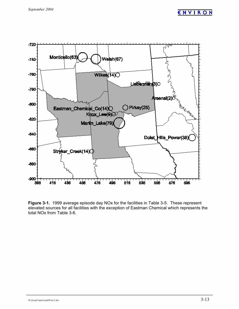
September 2004
H:\etcog3\report\sept04\sec3.doc 3-13
Figure 3-1. 1999 average episode day NOx for the facilities in Table 3-5. These represent elevated sources for all facilities with the exception of Eastman Chemical which represents the total NOx from Table 3-6.

September 2004
H:\etcog3\report\sept04\sec3.doc 3-14
Table 3-7. Texas gridded 1999 episode day emissions by major source type.
Episode Day Area
Off- road
On- road EGUs
OtherPoints
Off Shore
Ship-ping
Total Anthropo
genic Bio-
genic Total Tons NOx Friday, August 13 636 980 1396 1472 999 549 35 6066 1100 7166Saturday, August 14 619 949 971 1403 998 549 35 5524 1082 6606Sunday, August 15 602 877 747 1336 998 549 35 5144 1105 6249Monday, August 16 636 980 1441 1392 999 549 35 6032 1082 7114Tuesday, August 17 636 980 1425 1367 999 549 35 5990 1040 7030Wednesday, August 18 636 980 1422 1430 999 549 35 6051 1078 7129Thursday, August 19 636 980 1446 1457 1001 549 35 6103 1068 7171Friday, August 20 636 980 1429 1400 1001 549 35 6030 1052 7082Saturday, August 21 619 949 981 1304 1000 549 35 5436 1053 6489Sunday, August 22 602 877 735 1280 1000 549 35 5077 1010 6087Tons VOC Friday, August 13 1736 462 1057 20 538 189 1 4003 22087 26090Saturday, August 14 1395 850 797 19 509 189 1 3760 20527 24287Sunday, August 15 1197 836 674 20 509 189 1 3425 20445 23871Monday, August 16 1736 462 915 20 538 189 1 3861 19998 23859Tuesday, August 17 1736 462 904 20 538 189 1 3850 19290 23141Wednesday, August 18 1736 462 914 19 538 189 1 3859 20752 24611Thursday, August 19 1736 462 940 19 538 189 1 3886 21745 25631Friday, August 20 1736 462 1086 19 538 189 1 4032 20788 24819Saturday, August 21 1395 850 785 19 509 189 1 3747 19565 23312Sunday, August 22 1197 836 651 19 509 189 1 3402 18023 21426Tons CO Friday, August 13 958 5388 13259 230 825 126 5 20791 2270 23061Saturday, August 14 823 7770 10437 228 821 126 5 20210 2159 22368Sunday, August 15 690 7631 8948 230 821 126 5 18450 2128 20578Monday, August 16 958 5388 11384 228 825 126 5 18915 2078 20993Tuesday, August 17 958 5388 11347 228 825 126 5 18878 2005 20883Wednesday, August 18 958 5388 11546 218 825 126 5 19066 2136 21202Thursday, August 19 958 5388 11679 218 825 126 5 19199 2212 21412Friday, August 20 958 5388 13215 226 825 126 5 20744 2127 22871Saturday, August 21 823 7770 10202 222 821 126 5 19969 2045 22013Sunday, August 22 690 7631 8855 227 821 126 5 18354 1963 20317
Table 3-8. Summary of 1999 gridded emissions by major source type for states other than Texas.
Area Off-road On-road Points Anthropogenic
State Week day Sat Sun
Week Day Sat Sun
Week Day Sat Sun
Week Day Sat Sun
Total weekday
Total Sat
Total Sun
NOx Alabama 35 34 34 518 514 498 458 343 343 848 834 834 1858 1725 1708Arkansas 116 107 102 209 204 193 282 212 212 317 316 316 924 839 823Florida 7 7 6 35 39 35 116 87 87 206 206 206 365 339 335Georgia 72 68 66 192 173 150 637 478 478 514 509 509 1415 1228 1203Illinois 13 12 12 257 253 245 220 165 165 510 605 605 1000 1035 1028Indiana 33 30 29 153 144 133 240 180 180 802 810 810 1227 1164 1152Kansas 33 31 30 314 302 288 252 189 189 469 434 434 1068 956 940Kentucky 246 227 217 273 267 254 448 336 336 1032 1024 1024 1999 1854 1830Louisiana2 327 301 288 685 683 665 386 290 290 1171 1171 1121 2569 2445 2364Mississippi 6 6 6 220 217 206 354 266 266 529 529 529 1110 1018 1007Missouri 177 165 159 447 444 422 592 444 444 684 686 686 1900 1740 1711Nebraska 4 4 3 60 60 59 18 14 14 27 10 10 109 86 86North Carolina 1 1 1 3 2 2 21 16 16 13 13 13 38 32 31Ohio 24 22 21 99 92 84 131 98 98 653 651 651 907 863 854Oklahoma1,2 71 66 63 328 325 314 397 400 397 670 592 592 1467 1383 1366 South Carolina 0 0 0 0 0 0 3 2 2 0 0 0 4 3 3

September 2004
H:\etcog3\report\sept04\sec3.doc 3-15
Area Off-road On-road Points Anthropogenic
State Week day Sat Sun
Week Day Sat Sun
Week Day Sat Sun
Week Day Sat Sun
Total weekday
Total Sat
Total Sun
Tennessee 63 59 57 275 264 242 556 417 417 765 785 785 1657 1525 1502Virginia 1 1 1 4 4 4 9 7 7 2 0 0 17 12 12West Virginia 3 3 3 37 37 35 15 12 12 121 121 121 177 172 171Grand Total 1233 1143 1099 4112 4024 3828 5136 3954 3952 9331 9297 9247 19812 18419 18126VOC Alabama 491 491 491 140 345 342 345 259 259 207 166 166 1183 1260 1257Arkansas 381 381 381 82 201 199 185 139 139 97 84 84 745 804 802Florida 127 127 127 52 189 188 85 64 64 117 114 114 381 493 493Georgia 421 421 421 136 212 208 417 313 313 70 51 51 1044 997 993Illinois 208 208 208 63 114 113 136 102 102 87 69 69 494 493 492Indiana 279 279 279 54 95 93 160 120 120 82 53 53 575 546 544Kansas 318 317 317 84 128 126 173 129 129 85 52 52 659 626 624Kentucky 410 409 409 93 225 223 293 220 220 208 149 149 1004 1003 1001Louisiana2 420 419 419 150 421 418 246 184 184 258 273 272 1074 1297 1294Mississippi 427 427 427 80 219 218 207 155 155 168 165 165 882 967 966Missouri 922 921 921 205 491 487 387 290 290 125 95 95 1640 1798 1793Nebraska 44 44 44 9 13 13 11 8 8 3 3 3 68 69 69North Carolina 17 17 17 5 10 10 12 9 9 7 5 5 41 41 41Ohio 152 152 152 50 58 57 97 72 72 17 13 13 315 296 294Oklahoma1,2 311 310 310 97 219 217 416 402 414 106 97 97 929 1029 1039 South Carolina 2 2 2 1 1 1 2 1 1 0 0 0 4 5 5Tennessee 709 709 708 134 316 312 369 277 277 297 164 164 1509 1465 1461Virginia 8 8 8 1 1 1 6 4 4 2 0 0 16 13 13West Virginia 23 23 23 6 12 12 11 8 8 9 8 8 49 52 52Grand Total 5669 5667 5666 1438 3271 3239 3557 2758 2770 1948 1559 1559 12612 13255 13233CO Alabama 245 245 245 1195 1964 1929 3592 2694 2694 479 436 436 5512 5339 5304Arkansas 121 120 119 702 1154 1128 2027 1520 1520 297 293 293 3147 3087 3061Florida 60 60 60 358 744 736 859 644 644 601 600 600 1878 2049 2040Georgia 502 501 500 1851 2574 2524 4641 3481 3481 192 180 180 7186 6736 6684Illinois 38 38 37 680 929 912 1475 1107 1107 104 104 104 2297 2177 2160Indiana 93 92 92 685 903 879 1667 1250 1250 181 154 154 2626 2400 2375Kansas 87 84 83 1017 1346 1317 1870 1403 1403 248 235 235 3222 3068 3037Kentucky 200 197 195 897 1442 1413 3075 2306 2306 295 285 285 4467 4230 4199Louisiana2 182 178 177 1181 2097 2064 2742 2056 2056 855 873 871 4960 5204 5168Mississippi 125 125 125 647 1126 1103 2092 1569 1569 194 193 193 3058 3012 2989Missouri 372 369 368 2087 3231 3180 4002 3002 3002 311 306 306 6773 6908 6855Nebraska 3 3 3 94 126 124 122 91 91 4 3 3 223 223 221North Carolina 17 17 17 44 62 61 134 100 100 9 9 9 204 188 187Ohio 63 63 63 755 901 883 980 735 735 96 91 91 1894 1791 1773Oklahoma1,2 84 83 83 964 1488 1466 2846 2810 2848 192 186 186 4086 4568 4583South Carolina 3 3 3 4 7 7 20 15 15 0 0 0 28 25 25Tennessee 267 265 265 1374 2161 2112 3904 2928 2928 267 272 272 5812 5626 5577Virginia 5 5 5 11 14 14 61 45 45 1 1 1 78 65 65West Virginia 12 12 12 49 77 74 114 86 86 14 13 13 188 187 185
Grand Total 2480 2461 2451 14596 22345 21925 36222 27843 27880 4338 4234 4233 57637 56883 56489 1 For Oklahoma, On-road Weekday is Aug. 17, Saturday is Aug. 14, Sunday is Aug. 15 2 For Louisiana and Oklahoma, Point Sources with only day-specific data use Aug. 17 for Wkd, Aug. 14 for Sat and Aug. 15 for Sun

September 2004
H:\etcog3\report\sept04\sec3.doc 3-16
Table 3-9. Gridded biogenic emissions for states other than Texas. 13-Aug 14-Aug 15-Aug 16-Aug 17-Aug 18-Aug 19-Aug 20-Aug 21-Aug 22-Aug
NOx (tpd) Alabama 78 68 64 70 74 77 74 68 67 68Arkansas 128 96 94 109 126 134 129 103 102 112Florida 11 10 9 9 10 10 10 9 9 9Georgia 51 49 45 47 47 49 48 44 45 46Illinois 338 271 282 343 385 334 303 292 299 333Indiana 158 112 121 145 164 144 128 120 130 141Kansas 444 497 613 689 645 574 494 472 549 549Kentucky 154 108 113 139 160 149 143 118 122 134Louisiana 111 102 91 98 106 112 116 106 101 103Mississippi 133 108 99 113 127 133 137 116 110 118Missouri 245 215 242 300 314 294 250 235 250 270Nebraska 148 176 221 226 211 192 170 175 194 192North Carolina 2 1 1 1 2 1 2 1 1 1Ohio 22 17 18 20 25 20 19 17 18 20Oklahoma 196 195 220 238 232 233 202 187 208 216South Carolina 0 0 0 0 0 0 0 0 0 0Tennessee 122 86 87 107 120 122 118 93 94 103Virginia 1 1 0 1 1 1 1 0 0 1West Virginia 0 0 0 0 1 0 0 0 0 0NOX Totals 2342 2112 2322 2656 2750 2581 2342 2158 2301 2415VOC (tpd) Alabama 14097 11687 10261 11937 12969 14092 12878 11027 10796 10584Arkansas 11291 7772 7543 9151 11323 12454 11394 8109 8074 9278Florida 2772 2287 2158 2335 2424 2413 2501 2227 2391 2268Georgia 5614 5244 4760 5001 5229 5973 5539 4163 4471 4451Illinois 1692 982 1211 1758 1987 1250 1215 1236 1343 1558Indiana 1395 554 823 1163 1421 999 837 747 910 1067Kansas 973 1127 1674 2129 1944 1678 1204 1015 1365 1136Kentucky 3596 1383 1808 2922 3641 2991 2727 1654 2109 2645Louisiana 9282 8317 6817 7615 8392 8981 9574 8468 7649 7784Mississippi 14325 10911 9068 11206 12666 13599 13921 11249 10355 11261Missouri 7786 5601 7350 10521 11716 10253 7380 6513 7538 8222Nebraska 143 225 345 363 330 276 212 225 266 218North Carolina 602 497 414 512 568 547 565 367 356 388Ohio 210 86 113 170 234 163 122 110 133 423Oklahoma 6505 5351 5630 6046 6717 7195 6392 4891 5089 5953South Carolina 105 102 83 90 95 111 107 70 72 83Tennessee 8016 3911 4390 6723 7714 7522 7131 4132 4768 5342Virginia 98 62 46 91 109 91 82 46 50 71West Virginia 88 37 38 68 93 66 59 36 47 103VOC Totals 88590 66134 64531 79801 89572 90652 83840 66284 67781 72836CO (tpd) Alabama 1349 1141 1014 1143 1231 1328 1223 1092 1068 1073Arkansas 1030 752 705 834 1019 1132 1030 776 764 859Florida 354 313 282 301 309 313 312 291 300 295Georgia 517 457 411 433 451 495 474 381 391 401Illinois 166 108 117 155 180 149 136 123 127 146Indiana 145 82 93 123 147 118 101 90 101 118Kansas 136 149 205 257 241 210 155 143 176 173Kentucky 344 196 194 276 337 288 267 195 212 263Louisiana 953 882 722 791 872 934 1002 885 810 815Mississippi 1302 1022 847 1011 1142 1232 1246 1036 959 1037Missouri 610 470 551 742 842 801 594 524 574 630

September 2004
H:\etcog3\report\sept04\sec3.doc 3-17
13-Aug 14-Aug 15-Aug 16-Aug 17-Aug 18-Aug 19-Aug 20-Aug 21-Aug 22-AugNebraska 21 27 39 42 39 33 26 27 32 31North Carolina 54 44 38 45 48 46 49 36 33 37Ohio 20 12 12 16 21 15 13 11 13 51Oklahoma 559 472 489 529 574 624 538 435 470 537South Carolina 10 9 7 8 8 9 9 7 7 8Tennessee 692 427 419 584 668 650 621 439 440 480Virginia 9 7 5 8 10 8 8 5 5 7West Virginia 8 5 4 6 8 6 5 4 4 11CO Totals 8277 6575 6152 7304 8146 8392 7809 6499 6486 6972 DATA SOURCES FOR 2002 A 2002 emission inventory was developed because 2002 was the base year for the attainment demonstration, as discussed in Section 6. Point Sources Point source data for the 2002 inventory included: • 2002 3rd quarter Acid Rain data • 2000 Texas non-EGU point sources • 2002 Facility specific data • 1999 Texas minor point sources • 1999 NEIv2 point sources The point source data are processed for a typical peak ozone (PO) season weekday and weekend day. The point sources processed for the 1999 emissions modeling were the basis of the 2002 modeling point sources emissions. The following adjustments were made to the 1999 processing: 2002 emission estimates for Chemical Eastman Company were provided by NETAC. The 2002 3rd quarter average NOx emissions from the EPA Acid Rain database were extracted for Texas point specific EGUs. The other Texas point source data is based on the TCEQ 2000 PSDB provided by TCEQ in EPS2x AFS input format. (ftp://ftp.TCEQ.state.tx.us/pub/OEPAA/TAD/Modeling/file_transfer/HGPoints/2000/latlongv12. The Acid Rain NOx was removed from the TCEQ PSDB to avoid double counting of emissions. The 2002 3rd quarter average NOx emissions from the EPA Acid Rain database were also used for Louisiana, Arkansas and Oklahoma point specific EGUs. The corresponding NOx data was removed from the 1999 NEIv2 inventory to avoid double counting of emission. For all other states the 1999 NEIv2 was used to estimate 2002 emissions. The EGU data in the ozone season day inventory was adjusted so that each state total matched the 2002 3rd quarter average in the Acid Rain database. The non-EGU data was used at the 1999 levels.

September 2004
H:\etcog3\report\sept04\sec3.doc 3-18
The NOx criterion for selecting plume in grid treatment within the 4km modeling domain is 2 tons NOx on any day. For the regional emissions grid the NOx criterion is 25 tons per day. Mobile Sources The Texas Transportation Institute (TTI) prepared mobile source emissions for the counties within the East Texas NNA for 2002. Emission factors are from the EPA’s MOBILE6.2 model. Vehicle miles traveled (VMT) for 2002 are based on transportation modeling for Gregg and Smith counties and based on a rural HPMS for Rusk, Harrison and Upshur. All were prepared for four day-of-week scenarios (Weekday, Friday, Saturday and Sunday) and were adjusted to episode day temperature and humidities. All other Texas counties were based on the 1999 inventory developed by TTI for the four day-of-week scenarios adjusted for episode day temperature and humidities. This inventory was projected to 2002 levels with 2002 VMT and fleet turnover developed by TTI. The data were processed using the same methods described for 1999, above. This resulted in hourly specific mobile source emissions for all Texas counties. The other states are based on Mobile6.2 emission factors for typical summer day conditions (as used in the NEI99v2) with EPA data for 2002 VMT and fleet turnover. Area Sources The area emission estimates for Texas are based on the 1999 processing. The 1999 estimates are projected to 2002 estimates based on EGAS growth factors. The exception is for oil and gas production, which is projected, using the ratio of 2002 to 1999 production values. For all remaining states, the 1999 NEIv2 emission inventory is projected to 2002 estimates with EGAS growth factors. Off-Road Sources Off-road 2002 emissions estimates for the counties within the East Texas NNA were generated using NonRoadv2002 with local data for mining and construction equipment. Aircraft and railroad emissions estimated for 1999 were grown using EGAS growth factors. NonRoadv2002 with input data developed by TCEQ was run to estimate off-road emissions for the other Texas counties. The aircraft, commercial marine and railroad emissions are taken from the TCEQ 1999 off-road inventory and projected with EGAS growth factors. For all other states, NonRoadv2002 was used to estimate emissions. The aircraft, commercial marine and railroad emissions were taken from the 1999 NEI v2 inventory and projected to 2002 estimates using EGAS growth factors. The exception was for Oklahoma where the 1999 aircraft, commercial marine and railroad estimates provided by ODEQ were grown with EGAS growth factors.

September 2004
H:\etcog3\report\sept04\sec3.doc 3-19
Biogenic Sources The preparation of the biogenic emissions using GloBEIS version 3.1 is described at the end of Section 3. EMISSIONS SUMMARIES FOR 2002 All emission estimates in the following tables reflect gridded, model ready emissions. This means that for partial counties and/or states at the edge of a modeling domain, only the portion of emissions that is within the modeling domain is reported. Tables 3-10 to 3-12 are episode day emission summaries by major source type for the NNA counties and two Louisiana parishes. Table 3-13 indicates episode day NOx emissions for the elevated point sources within the 4km grid which have been selected for plume in grid treatment in CAMx modeling. Table 3-14 summarizes total NOx, elevated and surface, for Texas Eastman. Figure 3-2 displays the average episode day NOx for these sources. Table 3-15 lists new facilities in Northeast Texas; sources not present in the 1999 base year modeling. Table 3-16 represents total gridded Texas emissions for each episode day. Tables 3-17 and 3-18 summarize the gridded emissions by major source type for states other than Texas. Table 3-10. 2002 NOx for East Texas NNA and Shreveport area counties. 2002 NOx tons Episode Day Source
Gregg 48183
Harrison48203
Rusk 48401
Smith 48423
Upshur 48459
Bossier22015
Caddo 22017
Friday, August 13 Area 13.4 8.5 13.9 5.8 9.0 4.1 45.6 Off-road 4.4 5.7 2.4 6.3 2.2 2.8 5.9 On-road 20.8 17.2 3.8 24.2 2.7 7.1 19.7 Points 7.1 32.0 57.8 3.8 1.5 3.9 5.3 Subtotal 45.7 63.3 77.9 40.0 15.3 17.9 76.5 Biogenics 0.2 0.5 0.5 0.6 0.4 0.6 2.5 Total 45.9 63.8 78.4 40.6 15.8 18.6 79.0Saturday, August 14 Area 11.9 8.1 13.7 4.5 8.8 3.8 41.9 Off-road 3.9 5.1 1.9 5.7 2.1 2.5 5.3 On-road 14.9 12.8 3.1 17.5 2.0 5.3 14.8 Points 6.7 32.0 57.8 3.7 1.5 4.0 5.3 Subtotal 37.4 58.0 76.5 31.4 14.5 15.6 67.3 Biogenics 0.2 0.5 0.5 0.6 0.4 0.6 2.3 Total 37.6 58.4 77.0 32.0 14.9 16.2 69.6Sunday, August 15 Area 10.5 7.7 13.4 3.2 8.7 3.6 40.0 Off-road 3.3 4.3 1.4 5.0 2.1 2.0 4.4 On-road 10.8 9.4 2.5 13.1 1.9 5.3 14.8 Points 6.7 32.0 57.8 3.7 1.5 4.0 5.3 Subtotal 31.3 53.4 75.1 24.9 14.2 15.0 64.6 Biogenics 0.2 0.4 0.4 0.6 0.4 0.5 2.2 Total 31.4 53.8 75.5 25.5 14.5 15.5 66.7Monday, August 16 Area 13.4 8.5 13.9 5.8 9.0 4.1 45.6 Off-road 4.4 5.7 2.4 6.3 2.2 2.8 5.9
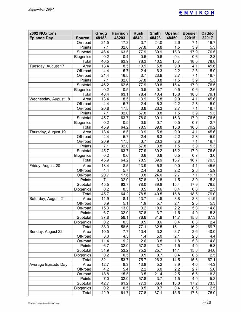
September 2004
H:\etcog3\report\sept04\sec3.doc 3-20
2002 NOx tons Episode Day Source
Gregg 48183
Harrison48203
Rusk 48401
Smith 48423
Upshur 48459
Bossier22015
Caddo 22017
On-road 21.5 17.3 3.7 24.0 2.6 7.1 19.7 Points 7.1 32.0 57.8 3.8 1.5 3.9 5.3 Subtotal 46.4 63.5 77.9 39.9 15.3 17.9 76.5 Biogenics 0.2 0.4 0.5 0.6 0.4 0.6 2.3 Total 46.5 63.9 78.3 40.5 15.7 18.5 78.8Tuesday, August 17 Area 13.4 8.5 13.9 5.8 9.0 4.1 45.6 Off-road 4.4 5.7 2.4 6.3 2.2 2.8 5.9 On-road 21.4 16.5 3.7 23.9 2.7 7.1 19.7 Points 7.1 32.0 57.8 3.8 1.5 3.9 5.3 Subtotal 46.2 62.6 77.9 39.8 15.4 17.9 76.5 Biogenics 0.2 0.5 0.5 0.7 0.5 0.6 2.6 Total 46.4 63.1 78.4 40.4 15.8 18.6 79.1Wednesday, August 18 Area 13.4 8.5 13.9 5.8 9.0 4.1 45.6 Off-road 4.4 5.7 2.4 6.3 2.2 2.8 5.9 On-road 20.8 17.5 3.8 23.3 2.7 7.1 19.7 Points 7.1 32.0 57.8 3.8 1.5 3.9 5.3 Subtotal 45.7 63.7 78.0 39.1 15.3 17.9 76.5 Biogenics 0.2 0.5 0.5 0.7 0.5 0.7 2.7 Total 45.9 64.2 78.5 39.8 15.8 18.6 79.2Thursday, August 19 Area 13.4 8.5 13.9 5.8 9.0 4.1 45.6 Off-road 4.4 5.7 2.4 6.3 2.2 2.8 5.9 On-road 20.9 17.5 3.7 23.3 2.6 7.1 19.7 Points 7.1 32.0 57.8 3.8 1.5 3.9 5.3 Subtotal 45.7 63.7 77.9 39.2 15.2 17.9 76.5 Biogenics 0.2 0.6 0.6 0.8 0.5 0.7 3.0 Total 45.9 64.2 78.5 39.9 15.7 18.7 79.5Friday, August 20 Area 13.4 8.5 13.9 5.8 9.0 4.1 45.6 Off-road 4.4 5.7 2.4 6.3 2.2 2.8 5.9 On-road 20.7 17.6 3.8 24.0 2.7 7.1 19.7 Points 7.1 32.0 57.8 3.8 1.5 3.9 5.3 Subtotal 45.5 63.7 78.0 39.8 15.4 17.9 76.5 Biogenics 0.2 0.5 0.5 0.6 0.4 0.6 2.5 Total 45.7 64.2 78.5 40.5 15.8 18.6 79.0Saturday, August 21 Area 11.9 8.1 13.7 4.5 8.8 3.8 41.9 Off-road 3.9 5.1 1.9 5.7 2.1 2.5 5.3 On-road 15.3 13.0 3.2 18.0 2.2 5.3 14.8 Points 6.7 32.0 57.8 3.7 1.5 4.0 5.3 Subtotal 37.8 58.1 76.6 31.9 14.7 15.6 67.3 Biogenics 0.2 0.5 0.5 0.6 0.4 0.6 2.4 Total 38.0 58.6 77.1 32.5 15.1 16.2 69.7Sunday, August 22 Area 10.5 7.7 13.4 3.2 8.7 3.6 40.0 Off-road 3.3 4.3 1.4 5.0 2.1 2.0 4.4 On-road 11.4 9.2 2.6 13.8 1.8 5.3 14.8 Points 6.7 32.0 57.8 3.7 1.5 4.0 5.3 Subtotal 31.9 53.2 75.2 25.7 14.1 15.0 64.6 Biogenics 0.2 0.5 0.5 0.7 0.4 0.6 2.5 Total 32.1 53.7 75.7 26.3 14.5 15.6 67.1Average Episode Day Area 12.7 8.3 13.8 5.2 8.9 4.0 44.3 Off-road 4.2 5.4 2.2 6.0 2.2 2.7 5.6 On-road 18.8 15.5 3.5 21.4 2.5 6.6 18.3 Points 7.0 32.0 57.8 3.7 1.5 4.0 5.3 Subtotal 42.7 61.2 77.3 36.4 15.0 17.2 73.5 Biogenics 0.2 0.5 0.5 0.7 0.4 0.6 2.5 Total 42.9 61.7 77.8 37.1 15.5 17.8 76.0

September 2004
H:\etcog3\report\sept04\sec3.doc 3-21
Table 3-11. 2002 VOC for East Texas NNA and Shreveport area counties. 2002 VOC tons Episode Day Source
Gregg 48183
Harrison 48203
Rusk 48401
Smith 48423
Upshur 48459
Bossier22015
Caddo 22017
Friday, August 13 Area 15.7 14.3 12.7 15.3 14.3 6.4 27.5 Off-road 2.3 1.1 0.8 3.6 0.4 1.5 4.3 On-road 5.6 5.6 3.1 9.0 2.0 5.1 15.0 Points 5.6 16.4 2.3 8.6 1.0 1.7 5.8 Subtotal 29.1 37.3 18.9 36.5 17.7 14.7 52.6 Biogenics 64.2 325.9 280.4 254.5 154.0 298.7 238.5 Total 93.3 363.2 299.3 291.0 171.6 313.4 291.2Saturday, August 14 Area 12.2 12.0 10.7 10.6 13.3 6.4 27.5 Off-road 2.7 2.2 1.6 5.2 0.6 2.3 7.0 On-road 5.4 4.4 2.6 8.6 2.5 3.8 11.3 Points 5.0 15.1 2.3 7.3 1.0 1.7 5.7 Subtotal 25.4 33.7 17.2 31.7 17.4 14.3 51.4 Biogenics 61.2 297.1 263.2 234.8 148.9 259.0 205.0 Total 86.6 330.8 280.4 266.4 166.3 273.3 256.4Sunday, August 15 Area 10.5 10.9 9.8 7.9 12.6 6.4 27.4 Off-road 2.6 2.1 1.6 5.0 0.6 2.2 6.8 On-road 5.6 4.5 3.5 9.0 1.8 3.8 11.3 Points 5.0 15.1 2.3 7.3 1.0 1.7 5.7 Subtotal 23.8 32.7 17.2 29.2 16.1 14.2 51.2 Biogenics 54.5 257.5 231.2 218.1 132.0 218.3 176.4 Total 78.3 290.2 248.4 247.4 148.0 232.5 227.6Monday, August 16 Area 15.7 14.3 12.7 15.3 14.3 6.4 27.5 Off-road 2.3 1.1 0.8 3.6 0.4 1.5 4.3 On-road 4.9 4.5 2.6 7.8 1.7 5.1 15.0 Points 5.6 16.4 2.3 8.6 1.0 1.7 5.8 Subtotal 28.4 36.2 18.4 35.3 17.4 14.7 52.6 Biogenics 57.9 276.2 240.2 228.2 140.2 236.6 185.4 Total 86.2 312.4 258.6 263.6 157.6 251.4 238.1Tuesday, August 17 Area 15.7 14.3 12.7 15.3 14.3 6.4 27.5 Off-road 2.3 1.1 0.8 3.6 0.4 1.5 4.3 On-road 5.2 6.2 2.6 8.4 1.7 5.1 15.0 Points 5.6 16.4 2.3 8.6 1.0 1.7 5.8 Subtotal 28.7 38.0 18.3 35.9 17.4 14.7 52.6 Biogenics 64.8 322.8 264.4 250.1 160.9 285.1 225.4 Total 93.5 360.7 282.8 286.0 178.3 299.8 278.0Wednesday, August 18 Area 15.7 14.3 12.7 15.3 14.3 6.4 27.5 Off-road 2.3 1.1 0.8 3.6 0.4 1.5 4.3 On-road 5.3 4.1 2.5 8.6 1.7 5.1 15.0 Points 5.6 16.4 2.3 8.6 1.0 1.7 5.8 Subtotal 28.8 35.8 18.3 36.1 17.4 14.7 52.6 Biogenics 70.0 343.6 292.5 273.6 168.8 312.2 242.7 Total 98.8 379.4 310.8 309.6 186.2 326.9 295.4Thursday, August 19 Area 15.7 14.3 12.7 15.3 14.3 6.4 27.5 Off-road 2.3 1.1 0.8 3.6 0.4 1.5 4.3 On-road 5.2 4.1 2.5 8.4 1.6 5.1 15.0 Points 5.6 16.4 2.3 8.6 1.0 1.7 5.8 Subtotal 28.7 35.8 18.3 35.9 17.3 14.7 52.6 Biogenics 76.7 377.5 316.4 299.0 184.4 339.1 267.8 Total 105.4 413.3 334.7 334.9 201.7 353.8 320.5Friday, August 20 Area 15.7 14.3 12.7 15.3 14.3 6.4 27.5 Off-road 2.3 1.1 0.8 3.6 0.4 1.5 4.3 On-road 6.4 5.1 2.8 10.3 2.1 5.1 15.0 Points 5.6 16.4 2.3 8.6 1.0 1.7 5.8

September 2004
H:\etcog3\report\sept04\sec3.doc 3-22
2002 VOC tons Episode Day Source
Gregg 48183
Harrison 48203
Rusk 48401
Smith 48423
Upshur 48459
Bossier22015
Caddo 22017
Subtotal 29.9 36.8 18.6 37.8 17.8 14.7 52.6 Biogenics 65.4 313.7 281.7 254.1 152.4 274.5 220.0 Total 95.3 350.5 300.3 291.9 170.1 289.2 272.7Saturday, August 21 Area 12.2 12.0 10.7 10.6 13.3 6.4 27.5 Off-road 2.7 2.2 1.6 5.2 0.6 2.3 7.0 On-road 5.6 4.3 2.5 9.0 1.6 3.8 11.3 Points 5.0 15.1 2.3 7.3 1.0 1.7 5.7 Subtotal 25.6 33.6 17.2 32.0 16.5 14.3 51.4 Biogenics 61.8 292.0 258.1 242.2 148.3 253.4 202.4 Total 87.4 325.6 275.3 274.3 164.8 267.7 253.8Sunday, August 22 Area 10.5 10.9 9.8 7.9 12.6 6.4 27.4 Off-road 2.6 2.1 1.6 5.0 0.6 2.2 6.8 On-road 5.3 4.7 2.4 8.5 1.5 3.8 11.3 Points 5.0 15.1 2.3 7.3 1.0 1.7 5.7 Subtotal 23.5 32.8 16.0 28.7 15.8 14.2 51.2 Biogenics 64.2 308.5 263.8 249.2 155.1 263.5 210.7 Total 87.7 341.3 279.8 277.9 170.8 277.7 261.9Average Episode Day Area 14.4 13.5 12.0 13.6 13.9 6.4 27.5 Off-road 2.4 1.4 1.0 4.0 0.5 1.7 5.0 On-road 5.4 4.7 2.7 8.6 1.8 4.7 14.0 Points 5.4 16.0 2.3 8.2 1.0 1.7 5.8 Subtotal 27.6 35.6 18.0 34.4 17.1 14.6 52.2 Biogenics 65.0 316.8 271.8 253.9 157.1 279.5 221.1 Total 92.6 352.4 289.8 288.4 174.2 294.1 273.4 Table 3-12. 2002 CO for East Texas NNA and Shreveport area counties. 2002 CO tons Episode Day Source
Gregg 48183
Harrison48203
Rusk 48401
Smith 48423
Upshur 48459
Bossier22015
Caddo22017
Friday, August 13 Area 3.8 7.2 8.5 8.6 5.6 7.4 13.9 Off-road 41.7 10.1 7.7 53.9 5.1 22.8 60.3 On-road 75.5 76.7 38.7 121.8 25.3 54.0 158.4 Points 5.3 11.1 6.6 2.0 0.9 1.8 2.7 Subtotal 126.2 105.1 61.6 186.4 36.9 85.9 235.2 Biogenics 5.6 29.9 27.1 22.8 14.6 26.6 21.1 Total 131.8 135.0 88.7 209.1 51.6 112.5 256.3Saturday, August 14 Area 3.3 6.5 7.9 6.9 5.1 7.3 13.3 Off-road 60.1 16.2 12.2 74.3 6.6 30.2 90.6 On-road 74.8 65.9 34.4 121.7 31.6 40.5 118.8 Points 4.9 11.1 6.6 1.9 0.9 1.8 2.7 Subtotal 143.1 99.8 61.0 204.9 44.2 79.8 225.4 Biogenics 5.6 28.8 27.0 22.4 14.7 23.9 19.3 Total 148.7 128.6 88.0 227.3 58.9 103.7 244.6Sunday, August 15 Area 2.8 5.9 7.3 5.2 4.5 7.3 13.0 Off-road 59.0 15.7 11.8 73.0 6.4 29.5 88.9 On-road 78.7 67.9 44.5 126.8 24.0 40.5 118.8 Points 4.9 11.1 6.6 1.9 0.9 1.8 2.7 Subtotal 145.4 100.6 70.2 207.0 35.9 79.0 223.4 Biogenics 5.0 25.1 23.7 20.5 13.0 20.6 16.8 Total 150.4 125.6 93.9 227.4 48.9 99.6 240.2Monday, August 16 Area 3.8 7.2 8.5 8.6 5.6 7.4 13.9 Off-road 41.7 10.1 7.7 53.9 5.1 22.8 60.3 On-road 61.6 61.2 31.5 101.6 21.3 54.0 158.4 Points 5.3 11.1 6.6 2.0 0.9 1.8 2.7
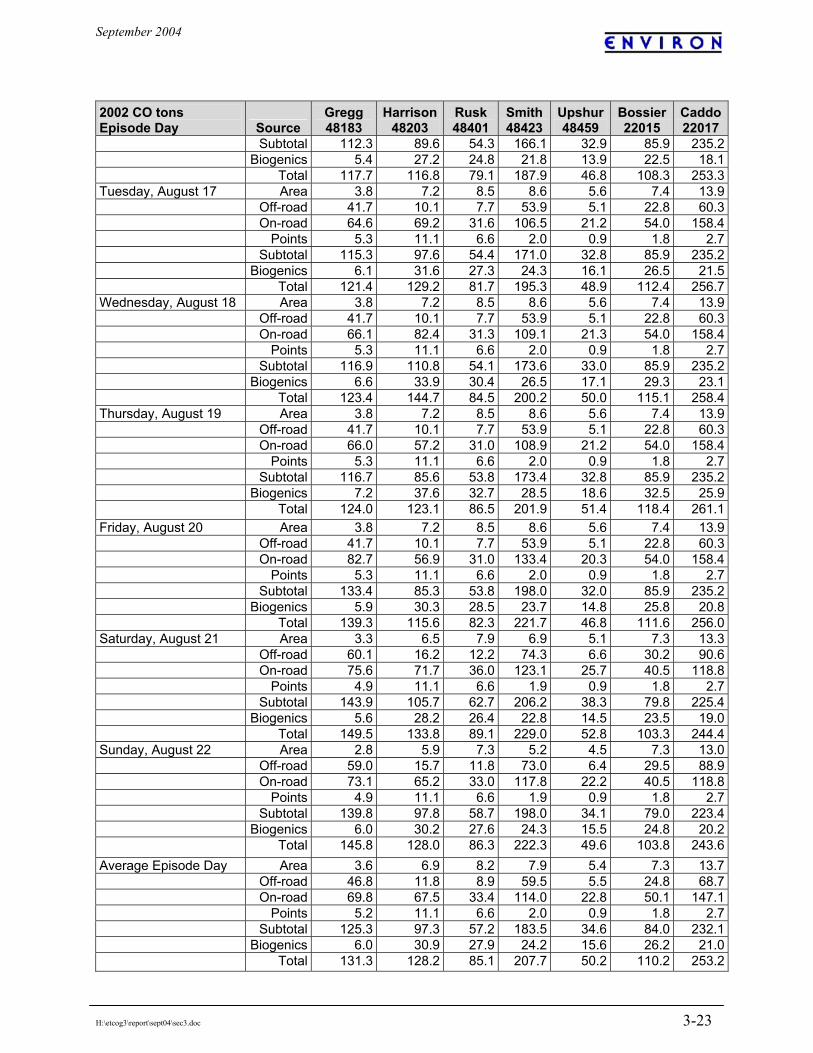
September 2004
H:\etcog3\report\sept04\sec3.doc 3-23
2002 CO tons Episode Day Source
Gregg 48183
Harrison48203
Rusk 48401
Smith 48423
Upshur 48459
Bossier22015
Caddo22017
Subtotal 112.3 89.6 54.3 166.1 32.9 85.9 235.2 Biogenics 5.4 27.2 24.8 21.8 13.9 22.5 18.1 Total 117.7 116.8 79.1 187.9 46.8 108.3 253.3Tuesday, August 17 Area 3.8 7.2 8.5 8.6 5.6 7.4 13.9 Off-road 41.7 10.1 7.7 53.9 5.1 22.8 60.3 On-road 64.6 69.2 31.6 106.5 21.2 54.0 158.4 Points 5.3 11.1 6.6 2.0 0.9 1.8 2.7 Subtotal 115.3 97.6 54.4 171.0 32.8 85.9 235.2 Biogenics 6.1 31.6 27.3 24.3 16.1 26.5 21.5 Total 121.4 129.2 81.7 195.3 48.9 112.4 256.7Wednesday, August 18 Area 3.8 7.2 8.5 8.6 5.6 7.4 13.9 Off-road 41.7 10.1 7.7 53.9 5.1 22.8 60.3 On-road 66.1 82.4 31.3 109.1 21.3 54.0 158.4 Points 5.3 11.1 6.6 2.0 0.9 1.8 2.7 Subtotal 116.9 110.8 54.1 173.6 33.0 85.9 235.2 Biogenics 6.6 33.9 30.4 26.5 17.1 29.3 23.1 Total 123.4 144.7 84.5 200.2 50.0 115.1 258.4Thursday, August 19 Area 3.8 7.2 8.5 8.6 5.6 7.4 13.9 Off-road 41.7 10.1 7.7 53.9 5.1 22.8 60.3 On-road 66.0 57.2 31.0 108.9 21.2 54.0 158.4 Points 5.3 11.1 6.6 2.0 0.9 1.8 2.7 Subtotal 116.7 85.6 53.8 173.4 32.8 85.9 235.2 Biogenics 7.2 37.6 32.7 28.5 18.6 32.5 25.9 Total 124.0 123.1 86.5 201.9 51.4 118.4 261.1Friday, August 20 Area 3.8 7.2 8.5 8.6 5.6 7.4 13.9 Off-road 41.7 10.1 7.7 53.9 5.1 22.8 60.3 On-road 82.7 56.9 31.0 133.4 20.3 54.0 158.4 Points 5.3 11.1 6.6 2.0 0.9 1.8 2.7 Subtotal 133.4 85.3 53.8 198.0 32.0 85.9 235.2 Biogenics 5.9 30.3 28.5 23.7 14.8 25.8 20.8 Total 139.3 115.6 82.3 221.7 46.8 111.6 256.0Saturday, August 21 Area 3.3 6.5 7.9 6.9 5.1 7.3 13.3 Off-road 60.1 16.2 12.2 74.3 6.6 30.2 90.6 On-road 75.6 71.7 36.0 123.1 25.7 40.5 118.8 Points 4.9 11.1 6.6 1.9 0.9 1.8 2.7 Subtotal 143.9 105.7 62.7 206.2 38.3 79.8 225.4 Biogenics 5.6 28.2 26.4 22.8 14.5 23.5 19.0 Total 149.5 133.8 89.1 229.0 52.8 103.3 244.4Sunday, August 22 Area 2.8 5.9 7.3 5.2 4.5 7.3 13.0 Off-road 59.0 15.7 11.8 73.0 6.4 29.5 88.9 On-road 73.1 65.2 33.0 117.8 22.2 40.5 118.8 Points 4.9 11.1 6.6 1.9 0.9 1.8 2.7 Subtotal 139.8 97.8 58.7 198.0 34.1 79.0 223.4 Biogenics 6.0 30.2 27.6 24.3 15.5 24.8 20.2 Total 145.8 128.0 86.3 222.3 49.6 103.8 243.6Average Episode Day Area 3.6 6.9 8.2 7.9 5.4 7.3 13.7 Off-road 46.8 11.8 8.9 59.5 5.5 24.8 68.7 On-road 69.8 67.5 33.4 114.0 22.8 50.1 147.1 Points 5.2 11.1 6.6 2.0 0.9 1.8 2.7 Subtotal 125.3 97.3 57.2 183.5 34.6 84.0 232.1 Biogenics 6.0 30.9 27.9 24.2 15.6 26.2 21.0 Total 131.3 128.2 85.1 207.7 50.2 110.2 253.2
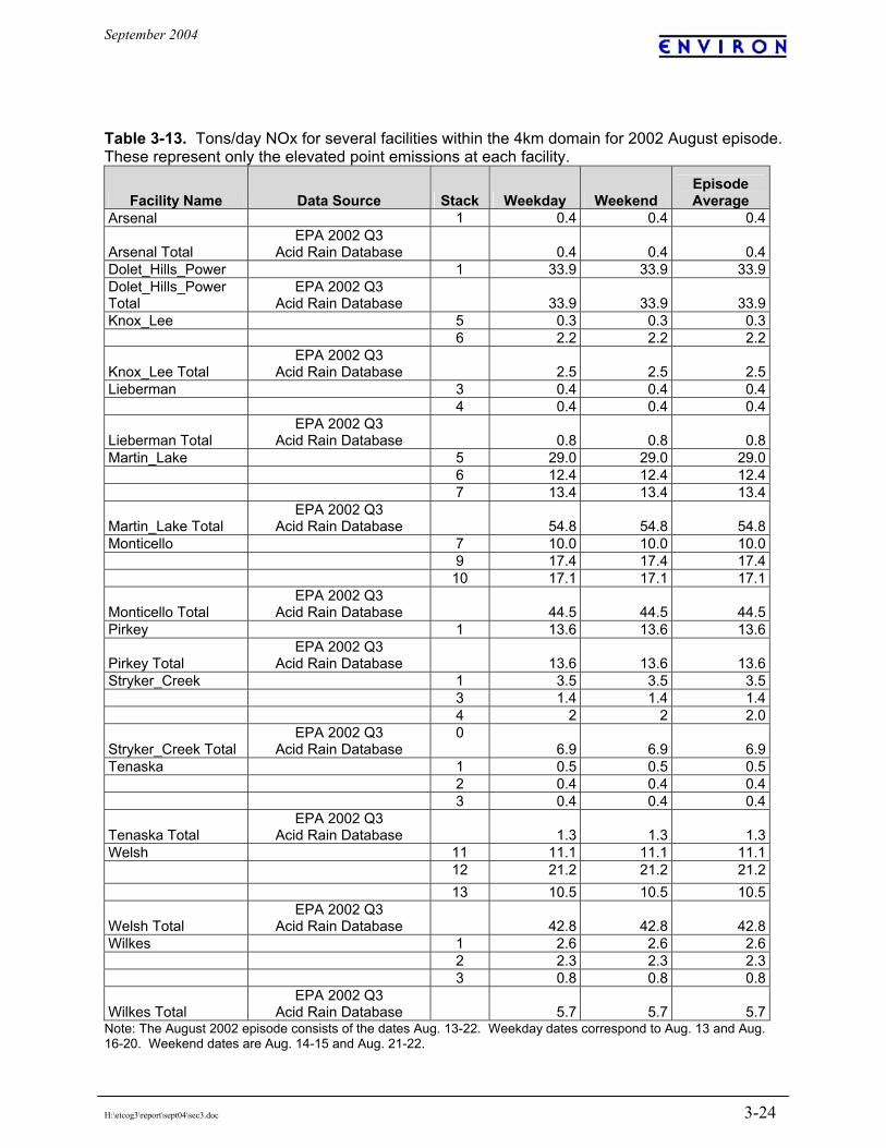
September 2004
H:\etcog3\report\sept04\sec3.doc 3-24
Table 3-13. Tons/day NOx for several facilities within the 4km domain for 2002 August episode. These represent only the elevated point emissions at each facility.
Facility Name Data Source Stack Weekday Weekend Episode Average
Arsenal 1 0.4 0.4 0.4
Arsenal Total EPA 2002 Q3
Acid Rain Database
0.4
0.4 0.4Dolet_Hills_Power 1 33.9 33.9 33.9Dolet_Hills_Power Total
EPA 2002 Q3 Acid Rain Database
33.9 33.9 33.9
Knox_Lee 5 0.3 0.3 0.3 6 2.2 2.2 2.2
Knox_Lee Total EPA 2002 Q3
Acid Rain Database
2.5 2.5 2.5Lieberman 3 0.4 0.4 0.4 4 0.4 0.4 0.4
Lieberman Total EPA 2002 Q3
Acid Rain Database
0.8 0.8 0.8Martin_Lake 5 29.0 29.0 29.0 6 12.4 12.4 12.4 7 13.4 13.4 13.4
Martin_Lake Total EPA 2002 Q3
Acid Rain Database
54.8 54.8 54.8Monticello 7 10.0 10.0 10.0 9 17.4 17.4 17.4 10 17.1 17.1 17.1
Monticello Total EPA 2002 Q3
Acid Rain Database
44.5 44.5 44.5Pirkey 1 13.6 13.6 13.6
Pirkey Total EPA 2002 Q3
Acid Rain Database
13.6 13.6 13.6Stryker_Creek 1 3.5 3.5 3.5 3 1.4 1.4 1.4 4 2 2 2.0
Stryker_Creek Total EPA 2002 Q3
Acid Rain Database 0
6.9 6.9 6.9Tenaska 1 0.5 0.5 0.5 2 0.4 0.4 0.4 3 0.4 0.4 0.4
Tenaska Total EPA 2002 Q3
Acid Rain Database
1.3 1.3 1.3Welsh 11 11.1 11.1 11.1 12 21.2 21.2 21.2 13 10.5 10.5 10.5
Welsh Total EPA 2002 Q3
Acid Rain Database
42.8 42.8 42.8Wilkes 1 2.6 2.6 2.6 2 2.3 2.3 2.3 3 0.8 0.8 0.8
Wilkes Total EPA 2002 Q3
Acid Rain Database
5.7 5.7 5.7Note: The August 2002 episode consists of the dates Aug. 13-22. Weekday dates correspond to Aug. 13 and Aug. 16-20. Weekend dates are Aug. 14-15 and Aug. 21-22.

September 2004
H:\etcog3\report\sept04\sec3.doc 3-25
Table 3-14. Eastman Chemical Co. total elevated and surface NOx tpd for average August 2002 episode day. The 'other' represents over a hundred individual stacks.
Cogen Unit
Stack 1 Cogen Unit
Stack 2 Other Elevated Other Surface Total NOx 1.05 1.05 6.2 1.0 9.3 VOC 0.0 0.0 0.9 10.8 11.8
Note: The cogen unit emissions are not actually Eastman Chemical Co. emissions, but are included in this table because Eastman agreed to offset the cogen emissions as part of their overall NOx reduction commitment. Table 3-15. 'New' point sources in Northeast Texas. Sources in the 2002 modeling which were not present in the 1999 base year modeling.
Facility Name County NOx Tenaska Rusk 1.3
Figure 3-2. 2002 average episode day NOx for the facilities in Table 3-13. These represent elevated sources for all facilities with the exception of Eastman Chemical which represents the total NOx from Table 3-14.

September 2004
H:\etcog3\report\sept04\sec3.doc 3-26
Table 3-16. Texas gridded 2002 episode day emissions by major source type.
Episode Day Area
Off- road
On- road EGUs
Other Points
Off Shore
Ship- ping
Total Anthro-pogenic
Bio- genic Total
Tons NOx Friday, August 13 647 934 1281 781 871 549 37 5100 1100 6200Saturday, August 14 629 910 894 781 871 549 37 4671 1082 5753Sunday, August 15 611 841 686 781 871 549 37 4376 1105 5481Monday, August 16 647 934 1317 781 871 549 37 5136 1082 6218Tuesday, August 17 647 934 1305 781 871 549 37 5124 1040 6164Wednesday, August 18 647 934 1303 781 871 549 37 5122 1078 6200Thursday, August 19 647 934 1322 781 871 549 37 5142 1068 6209Friday, August 20 647 934 1315 781 871 549 37 5134 1052 6186Saturday, August 21 629 910 899 781 871 549 37 4677 1053 5730Sunday, August 22 611 841 676 781 871 549 37 4366 1010 5376Tons VOC Friday, August 13 1816 447 898 20 485 189 1 3856 22087 25943Saturday, August 14 1441 823 665 20 460 189 1 3599 20527 24126Sunday, August 15 1227 810 563 20 460 189 1 3271 20445 23716Monday, August 16 1816 447 775 20 485 189 1 3734 19998 23732Tuesday, August 17 1816 447 766 20 485 189 1 3725 19290 23015Wednesday, August 18 1816 447 774 20 485 189 1 3733 20752 24485Thursday, August 19 1816 447 798 20 485 189 1 3756 21745 25501Friday, August 20 1816 447 922 20 485 189 1 3881 20788 24668Saturday, August 21 1441 823 653 20 460 189 1 3587 19565 23152Sunday, August 22 1227 810 556 20 460 189 1 3264 18023 21287Tons CO Friday, August 13 969 5704 11950 219 702 126 6 19676 2270 21946Saturday, August 14 832 8251 9233 219 699 126 6 19366 2159 21525Sunday, August 15 699 8121 7944 219 699 126 6 17814 2128 19941Monday, August 16 969 5704 10273 219 702 126 6 17999 2078 20077Tuesday, August 17 969 5704 10234 219 702 126 6 17960 2005 19965Wednesday, August 18 969 5704 10393 219 702 126 6 18119 2136 20254Thursday, August 19 969 5704 10485 219 702 126 6 18210 2212 20423Friday, August 20 969 5704 11884 219 702 126 6 19610 2127 21737Saturday, August 21 832 8251 9027 219 699 126 6 19161 2045 21206Sunday, August 22 699 8121 7991 219 699 126 6 17860 1963 19823
Table 3-17. Summary of August 2002 gridded emissions by major source type for states other than Texas. Area Off-road On-road Point Anthropogenic
State
Weekday Sat Sun Weekday Sat Sun
Weekday Sat Sun
Weekday Sat Sun
Total Week day
Total Sat
TotalSun
NOx Alabama 37 36 35 481 484 468 436 327 327 673 659 659 1626 1505 1488Arkansas 121 112 107 152 151 140 265 199 199 335 334 334 874 796 780Florida 7 7 7 31 40 35 114 85 85 186 186 186 338 317 313Georgia 74 70 68 156 141 118 627 470 470 336 331 331 1193 1013 987Illinois 13 13 12 206 204 197 203 152 152 339 388 388 761 756 748Indiana 33 31 30 141 134 123 220 165 165 642 647 647 1037 978 966Kansas 35 32 31 231 221 207 238 178 178 466 431 431 969 862 847Kentucky 255 235 225 230 228 215 417 312 312 677 671 671 1579 1447 1423Louisiana 343 315 302 671 678 661 364 273 273 941 939 939 2319 2205 2174Mississippi 6 6 6 193 195 184 321 241 241 422 422 422 942 864 853Missouri 181 169 162 352 359 336 553 415 415 529 531 531 1616 1473 1444Nebraska 4 4 4 40 39 39 16 12 12 28 10 10 87 65 64North Carolina 1 1 1 3 3 2 18 14 14 13 13 13 35 30 30Ohio 25 23 22 94 88 80 125 94 94 568 566 566 813 770 762Oklahoma 74 68 65 311 312 302 368 276 276 530 548 548 1282 1204 1190
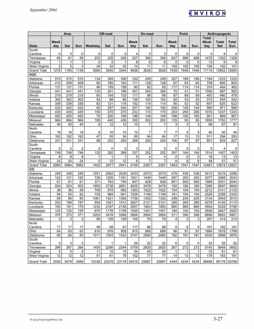
September 2004
H:\etcog3\report\sept04\sec3.doc 3-27
Area Off-road On-road Point Anthropogenic
State
Weekday Sat Sun Weekday Sat Sun
Weekday Sat Sun
Weekday Sat Sun
Total Week day
Total Sat
TotalSun
South Carolina 0 0 0 0 0 0 4 3 3 0 0 0 5 4 4Tennessee 65 61 59 232 228 206 527 395 395 647 668 668 1470 1352 1328Virginia 1 1 1 2 2 1 8 6 6 2 0 0 13 9 9West Virginia 3 3 3 34 33 32 14 11 11 105 105 105 156 152 151Grand Total 1278 1185 1139 3560 3540 3344 4838 3628 3628 7439 7448 7448 17115 15802 15560VOC Alabama 510 510 510 134 309 306 332 249 249 207 166 166 1184 1233 1230Arkansas 410 409 409 80 185 183 171 128 128 97 84 84 758 806 804Florida 131 131 131 46 159 158 80 60 60 117 114 114 374 464 463Georgia 441 441 441 133 201 196 407 305 305 70 51 51 1050 997 993Illinois 219 219 219 60 104 103 117 88 88 87 69 69 483 480 478Indiana 302 302 302 54 88 86 136 102 102 82 53 53 573 544 542Kansas 338 338 338 82 121 118 152 114 114 85 52 52 657 625 622Kentucky 422 422 422 93 207 204 257 192 192 208 149 149 980 971 968Louisiana 435 435 435 150 378 375 232 174 174 253 260 260 1070 1247 1243Mississippi 455 455 455 79 200 199 198 149 149 168 165 165 901 969 967Missouri 984 984 984 195 440 436 350 263 263 125 95 95 1655 1782 1777Nebraska 45 45 45 8 12 12 10 7 7 3 3 3 66 67 67North Carolina 18 18 18 5 10 10 10 7 7 7 5 5 40 40 40Ohio 162 162 162 47 55 54 85 64 64 17 13 13 311 294 293Oklahoma 331 331 331 98 202 200 266 200 200 106 97 97 801 829 827South Carolina 2 2 2 0 0 0 3 2 2 0 0 0 5 4 4Tennessee 749 748 748 132 292 288 337 252 252 297 164 164 1514 1457 1453Virginia 8 8 8 1 1 1 5 4 4 2 0 0 16 13 13West Virginia 24 24 24 5 12 12 9 7 7 9 8 8 48 51 51Grand Total 5985 5984 5983 1402 2977 2941 3156 2367 2367 1943 1547 1547 12487 12874 12837CO Alabama 246 246 246 1251 2062 2029 3433 2575 2575 479 436 436 5410 5319 5286Arkansas 122 121 120 726 1205 1181 1931 1449 1449 297 293 293 3077 3068 3043Florida 61 61 61 371 763 755 837 628 628 601 600 600 1869 2051 2044Georgia 504 503 502 1955 2738 2691 4635 3476 3476 192 180 180 7286 6897 6849Illinois 38 38 38 708 978 962 1363 1022 1022 104 104 104 2212 2141 2125Indiana 94 93 92 725 964 941 1529 1146 1146 181 154 154 2528 2358 2335Kansas 89 86 85 1061 1421 1392 1736 1302 1302 248 235 235 3134 3044 3014Kentucky 203 199 197 954 1541 1512 2827 2121 2121 295 285 285 4279 4145 4115Louisiana 185 181 179 1232 2187 2156 2657 1993 1993 860 869 869 4934 5229 5196Mississippi 125 125 125 675 1178 1156 1935 1451 1451 194 193 193 2928 2947 2925Missouri 376 373 371 2203 3418 3369 3806 2854 2854 311 306 306 6696 6952 6901Nebraska 3 3 3 95 129 128 105 79 79 4 3 3 207 214 213North Carolina 17 17 17 48 68 67 117 88 88 9 9 9 191 182 181Ohio 64 63 63 810 976 959 915 686 686 96 91 91 1884 1816 1799Oklahoma 85 84 83 1011 1563 1542 2747 2060 2060 192 191 191 4034 3898 3876South Carolina 3 3 3 1 1 1 29 22 22 0 0 0 33 25 25Tennessee 268 267 266 1450 2290 2244 3759 2820 2820 267 272 272 5745 5649 5602Virginia 5 5 5 11 15 15 54 40 40 1 1 1 72 61 61West Virginia 12 12 12 51 81 79 102 77 77 14 13 13 179 183 181
Grand Total 2500 2479 2469 15338 23578 23178 34516 25887 25887 4344 4234 4234 56698 56178 55768
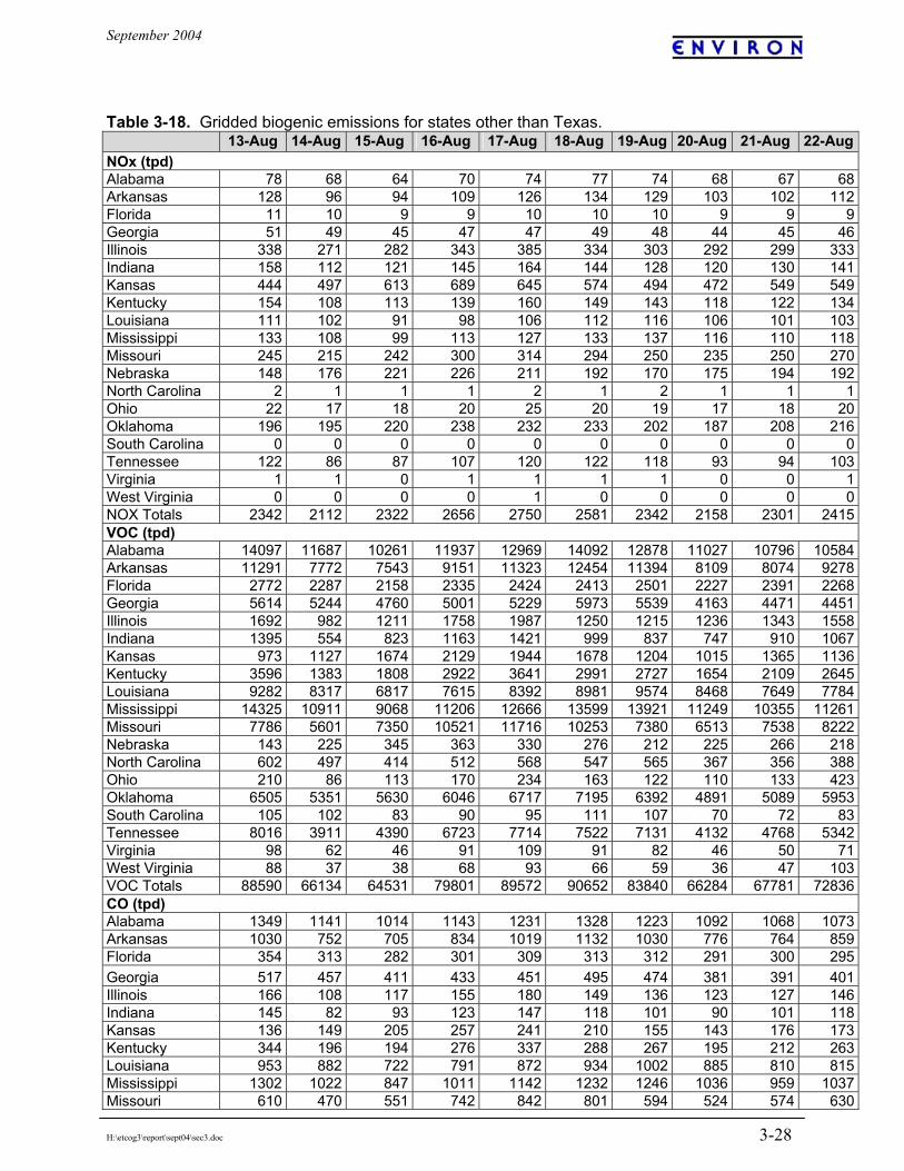
September 2004
H:\etcog3\report\sept04\sec3.doc 3-28
Table 3-18. Gridded biogenic emissions for states other than Texas. 13-Aug 14-Aug 15-Aug 16-Aug 17-Aug 18-Aug 19-Aug 20-Aug 21-Aug 22-Aug
NOx (tpd) Alabama 78 68 64 70 74 77 74 68 67 68Arkansas 128 96 94 109 126 134 129 103 102 112Florida 11 10 9 9 10 10 10 9 9 9Georgia 51 49 45 47 47 49 48 44 45 46Illinois 338 271 282 343 385 334 303 292 299 333Indiana 158 112 121 145 164 144 128 120 130 141Kansas 444 497 613 689 645 574 494 472 549 549Kentucky 154 108 113 139 160 149 143 118 122 134Louisiana 111 102 91 98 106 112 116 106 101 103Mississippi 133 108 99 113 127 133 137 116 110 118Missouri 245 215 242 300 314 294 250 235 250 270Nebraska 148 176 221 226 211 192 170 175 194 192North Carolina 2 1 1 1 2 1 2 1 1 1Ohio 22 17 18 20 25 20 19 17 18 20Oklahoma 196 195 220 238 232 233 202 187 208 216South Carolina 0 0 0 0 0 0 0 0 0 0Tennessee 122 86 87 107 120 122 118 93 94 103Virginia 1 1 0 1 1 1 1 0 0 1West Virginia 0 0 0 0 1 0 0 0 0 0NOX Totals 2342 2112 2322 2656 2750 2581 2342 2158 2301 2415VOC (tpd) Alabama 14097 11687 10261 11937 12969 14092 12878 11027 10796 10584Arkansas 11291 7772 7543 9151 11323 12454 11394 8109 8074 9278Florida 2772 2287 2158 2335 2424 2413 2501 2227 2391 2268Georgia 5614 5244 4760 5001 5229 5973 5539 4163 4471 4451Illinois 1692 982 1211 1758 1987 1250 1215 1236 1343 1558Indiana 1395 554 823 1163 1421 999 837 747 910 1067Kansas 973 1127 1674 2129 1944 1678 1204 1015 1365 1136Kentucky 3596 1383 1808 2922 3641 2991 2727 1654 2109 2645Louisiana 9282 8317 6817 7615 8392 8981 9574 8468 7649 7784Mississippi 14325 10911 9068 11206 12666 13599 13921 11249 10355 11261Missouri 7786 5601 7350 10521 11716 10253 7380 6513 7538 8222Nebraska 143 225 345 363 330 276 212 225 266 218North Carolina 602 497 414 512 568 547 565 367 356 388Ohio 210 86 113 170 234 163 122 110 133 423Oklahoma 6505 5351 5630 6046 6717 7195 6392 4891 5089 5953South Carolina 105 102 83 90 95 111 107 70 72 83Tennessee 8016 3911 4390 6723 7714 7522 7131 4132 4768 5342Virginia 98 62 46 91 109 91 82 46 50 71West Virginia 88 37 38 68 93 66 59 36 47 103VOC Totals 88590 66134 64531 79801 89572 90652 83840 66284 67781 72836CO (tpd) Alabama 1349 1141 1014 1143 1231 1328 1223 1092 1068 1073Arkansas 1030 752 705 834 1019 1132 1030 776 764 859Florida 354 313 282 301 309 313 312 291 300 295Georgia 517 457 411 433 451 495 474 381 391 401Illinois 166 108 117 155 180 149 136 123 127 146Indiana 145 82 93 123 147 118 101 90 101 118Kansas 136 149 205 257 241 210 155 143 176 173Kentucky 344 196 194 276 337 288 267 195 212 263Louisiana 953 882 722 791 872 934 1002 885 810 815Mississippi 1302 1022 847 1011 1142 1232 1246 1036 959 1037Missouri 610 470 551 742 842 801 594 524 574 630

September 2004
H:\etcog3\report\sept04\sec3.doc 3-29
13-Aug 14-Aug 15-Aug 16-Aug 17-Aug 18-Aug 19-Aug 20-Aug 21-Aug 22-AugNebraska 21 27 39 42 39 33 26 27 32 31North Carolina 54 44 38 45 48 46 49 36 33 37Ohio 20 12 12 16 21 15 13 11 13 51Oklahoma 559 472 489 529 574 624 538 435 470 537South Carolina 10 9 7 8 8 9 9 7 7 8Tennessee 692 427 419 584 668 650 621 439 440 480Virginia 9 7 5 8 10 8 8 5 5 7West Virginia 8 5 4 6 8 6 5 4 4 11CO Totals 8277 6575 6152 7304 8146 8392 7809 6499 6486 6972 DATA SOURCES FOR 2007 Point Sources Point source data were obtained from several different sources, processed separately and merged prior to modeling. The data include: • Texas electric generating units (EGUs) • Texas non-EGU point sources • Facility specific data • Texas minor point sources • Other State point sources The point source data are processed for a typical peak ozone (PO) season weekday and weekend day. The 2007 Texas point source data were provided by TCEQ in EPS2x AFS input format. The hourly EGU data are developed from the EPA’s Acid Rain Program Database and are based on 30-day peaks at each facility in the summer quarter of 1997, 1998 and 1999. These data include ‘new’ sources within 100 miles of the non-attainment areas. Controls are applied to the EGU data to represent TCEQ’s NOx rules. The TCEQ Point Source Data Base (PSDB) is the basis of the non-EGU Texas data. These data were provided as 2007 estimates and incorporated growth and controls. The files which were downloaded from the TCEQ ftp site ftp://ftp.TCEQ.state.tx.us/pub/AirQuality/AirQualityPlanningAssessment/Modeling/file_transfer/HGPoints/forDec2000SIP/ are:
TX EGU hourly_NAA30dayTXegu.afs_newEGU100miDFWandHGA_11 TX Non-EGU afs.tx_negu.930905-930911_12.tier2_07.NewNEGU.new
Many facilities in the Northeast Texas region provided future year emission estimates in developing the Northeast Texas Region Ozone SIP Revision (March, 2002) which are used in this modeling inventory. These sources were removed from the Texas files listed above and replaced with the provided SIP data. In addition, permits for new EGU units in the Northeast Texas region were researched and emission estimates were provided via email from TCEQ’s Ron Thomas.
September 2004
H:\etcog3\report\sept04\sec3.doc 3-30
For all states other than Texas the U.S. EPA 2007 national inventories developed to assist future modeling of the Heavy-Duty Engine and Vehicle Standards and Highway Diesel Fuel, henceforth referred to as 2007 HDD inventory, were downloaded from EPA’s ftp site.
ftp://ftp.epa.gov/EmisInventory/HDD_Rule/2007BaseCase/ Regional EGU Egu/eg07ms2h.zip Regional Non-EGU NonEGUPoint/pt07ms2h.zip
The compressed files (.zip) contain a Dbase/FoxPro formatted file (.dbf) which were converted to Ascii text (.dat) for processing. The data is processed to (1) extract peak ozone season data for those states within the regional modeling domain other than Texas, (2) reformatted to EPS2x AFS input file format and (3) processed through EPS2x. The 2007 HDD inventories are described in detail in Procedures for Developing Base Year and Future Year Mass and Modeling Inventories for the Heavy-Duty Engine and Vehicle Standards and Highway Diesel Fuel (HDD) Rulemaking (ftp://ftp.epa.gov/EmisInventory/HDD_Rule/ProceduresDocument/ProcRptFinal.wpd). The NOx criterion for selecting plume in grid treatment within the 4km modeling domain is 2 tons NOx on any day. For the regional emissions grid the NOx criterion is 25 tons per day. Mobile Sources The Texas Transportation Institute (TTI) prepared mobile source emissions for all Texas counties under contract to the TCEQ. Emission factors are from the EPA’s MOBILE6 model. Vehicle miles traveled (VMT) for 2007 are based on transportation models in all NNA counties that have a complete transportation model and were based on a rural HPMS method elsewhere. The NNA counties for which link based transportation model data are used:
East Texas: Gregg, Smith Austin: Hays, Travis, Williamson San Antonio: Bexar Corpus Christi: Nueces, San Patricio Victoria: Victoria
The 2007 TTI data were processed using the same methods described for 1999, above. The result of this processing was a mobile emissions inventory that accurately reflects the temperature and humidity in a given county during the modeling period. The other states are based on Mobile6.2 emission factors for typical summer day conditions (as used in the NEI99v2) with EPA data for 2007 VMT and fleet turnover.

September 2004
H:\etcog3\report\sept04\sec3.doc 3-31
Area Sources Area 1999 emissions estimates for the counties within the East Texas NNA were provided by Pollution Solutions. Refer to “Tyler/Longview/Marshall Flexible Attainment Region Emission Inventory Ozone Precursors, VOC, NOx and CO 1999 Emissions” May, 2002 for a detailed description of the inventory development. These data were provided via email by Jerry Demo of Pollution Solutions. The 1999 TCEQ area source data outside the East Texas NNA is the basis of the other Texas counties. The area source data were grown to 2007 estimates with factors by source classification code generated using EGAS 4.0. The exception is for oil and gas production which is projected using the ratio of 2007 to 1999 production values. In addition, control factors were applied by county based on the documented SIP rules in Coulter-Burke, et al., (2002). For all remaining areas, EPA’s 2007 HDD inventories are the basis for the area regional emissions inventory. The HDD 2007 area emission inventory is (1) processed to extract the typical peak ozone season day data, (2) reformatted to the EPS2x AMS input file format and (3) processed through EPS2x.
ftp://ftp.epa.gov/EmisInventory/HDD_Rule/2007BaseCase/Area_Nonroad Regional Area ar07ms2h.zip
Off-Road Sources Off-road 2007 emissions estimates for the counties within the East Texas NNA were generated using NonRoadv2002 with local data for mining and construction equipment. Aircraft and railroad emissions estimated for 1999 were grown using EGAS growth factors. NonRoadv2002 with input data developed by TCEQ was run to estimate off-road emissions for the other Texas counties. The aircraft, commercial marine and railroad emissions are taken from the TCEQ 1999 off-road inventory and projected with EGAS growth factors. For all other states, NonRoadv2002 was used to estimate emissions. The aircraft, commercial marine and railroad emissions were taken from EPA’s 2007 HDD off-road inventory. The HDD 2007 off-road emission inventory is (1) processed to extract the typical peak ozone season day data, (2) reformatted to the EPS2x AMS input file format and (3) processed through EPS2x.
ftp://ftp.epa.gov/EmisInventory/HDD_Rule/2007ControlCase/Area_Nonroad Regional Non-road n7ms1hc.zip
Biogenic Sources Biogenic emissions were prepared using version 3.1 of the GloBEIS model (Yarwood et al., 2002). These data were developed for the 1999 base case modeling and are identical for the 2007 modeling inventory.
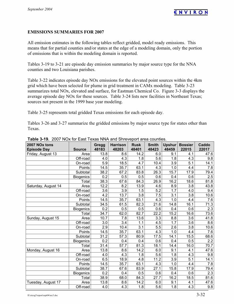
September 2004
H:\etcog3\report\sept04\sec3.doc 3-32
EMISSIONS SUMMARIES FOR 2007 All emission estimates in the following tables reflect gridded, model ready emissions. This means that for partial counties and/or states at the edge of a modeling domain, only the portion of emissions that is within the modeling domain is reported. Tables 3-19 to 3-21 are episode day emission summaries by major source type for the NNA counties and two Louisiana parishes. Table 3-22 indicates episode day NOx emissions for the elevated point sources within the 4km grid which have been selected for plume in grid treatment in CAMx modeling. Table 3-23 summarizes total NOx, elevated and surface, for Eastman Chemical Co. Figure 3-3 displays the average episode day NOx for these sources. Table 3-24 lists new facilities in Northeast Texas; sources not present in the 1999 base year modeling. Table 3-25 represents total gridded Texas emissions for each episode day. Tables 3-26 and 3-27 summarize the gridded emissions by major source type for states other than Texas. Table 3-19. 2007 NOx for East Texas NNA and Shreveport area counties. 2007 NOx tons Episode Day Source
Gregg 48183
Harrison48203
Rusk 48401
Smith 48423
Upshur 48459
Bossier22015
Caddo 22017
Friday, August 13 Area 13.8 8.6 14.2 6.0 9.1 4.1 47.6 Off-road 4.0 4.3 1.8 5.6 1.8 4.3 9.8 On-road 5.9 18.5 4.7 10.4 3.9 5.1 14.1 Points 14.5 35.7 63.1 4.3 1.0 4.4 7.8 Subtotal 38.2 67.2 83.8 26.3 15.7 17.9 79.4 Biogenics 0.2 0.5 0.5 0.6 0.4 0.6 2.5 Total 38.3 67.6 84.3 26.9 16.2 18.6 81.8Saturday, August 14 Area 12.2 8.2 13.9 4.6 8.9 3.8 43.8 Off-road 3.6 3.9 1.5 5.2 1.7 4.0 9.4 On-road 4.2 13.7 3.8 7.5 3.1 3.8 10.6 Points 14.5 35.7 63.1 4.3 1.0 4.4 7.6 Subtotal 34.5 61.5 82.3 21.6 14.8 16.1 71.3 Biogenics 0.2 0.5 0.5 0.6 0.4 0.6 2.3 Total 34.7 62.0 82.7 22.2 15.2 16.6 73.6Sunday, August 15 Area 10.7 7.8 13.6 3.3 8.8 3.6 41.8 Off-road 3.0 3.4 1.1 4.5 1.7 3.6 8.6 On-road 2.9 10.4 3.1 5.5 2.6 3.8 10.6 Points 14.5 35.7 63.1 4.3 1.0 4.4 7.6 Subtotal 31.2 57.3 80.9 17.5 14.1 15.5 68.6 Biogenics 0.2 0.4 0.4 0.6 0.4 0.5 2.2 Total 31.4 57.7 81.3 18.1 14.4 16.0 70.7Monday, August 16 Area 13.8 8.6 14.2 6.0 9.1 4.1 47.6 Off-road 4.0 4.3 1.8 5.6 1.8 4.3 9.8 On-road 6.5 18.9 4.8 11.2 3.9 5.1 14.1 Points 14.5 35.7 63.1 4.3 1.0 4.4 7.8 Subtotal 38.7 67.6 83.9 27.1 15.8 17.9 79.4 Biogenics 0.2 0.4 0.5 0.6 0.4 0.6 2.3 Total 38.9 68.0 84.3 27.7 16.2 18.5 81.6Tuesday, August 17 Area 13.8 8.6 14.2 6.0 9.1 4.1 47.6 Off-road 4.0 4.3 1.8 5.6 1.8 4.3 9.8

September 2004
H:\etcog3\report\sept04\sec3.doc 3-33
2007 NOx tons Episode Day Source
Gregg 48183
Harrison48203
Rusk 48401
Smith 48423
Upshur 48459
Bossier22015
Caddo 22017
On-road 6.5 18.9 4.8 11.1 4.0 5.1 14.1 Points 14.5 35.7 63.1 4.3 1.0 4.4 7.8 Subtotal 38.7 67.5 83.9 27.1 15.8 17.9 79.4 Biogenics 0.2 0.5 0.5 0.7 0.5 0.6 2.6 Total 38.9 68.0 84.4 27.7 16.3 18.6 81.9Wednesday, August 18 Area 13.8 8.6 14.2 6.0 9.1 4.1 47.6 Off-road 4.0 4.3 1.8 5.6 1.8 4.3 9.8 On-road 6.1 18.8 4.8 10.5 3.9 5.1 14.1 Points 14.5 35.7 63.1 4.3 1.0 4.4 7.8 Subtotal 38.3 67.4 83.9 26.4 15.8 17.9 79.4 Biogenics 0.2 0.5 0.5 0.7 0.5 0.7 2.7 Total 38.5 67.9 84.4 27.1 16.2 18.6 82.1Thursday, August 19 Area 13.8 8.6 14.2 6.0 9.1 4.1 47.6 Off-road 4.0 4.3 1.8 5.6 1.8 4.3 9.8 On-road 6.4 18.8 4.8 11.1 3.9 5.1 14.1 Points 14.5 35.7 63.1 4.3 1.0 4.4 7.8 Subtotal 38.7 67.4 83.8 27.0 15.7 17.9 79.4 Biogenics 0.2 0.6 0.6 0.8 0.5 0.7 3.0 Total 38.9 68.0 84.4 27.8 16.3 18.7 82.3Friday, August 20 Area 13.8 8.6 14.2 6.0 9.1 4.1 47.6 Off-road 4.0 4.3 1.8 5.6 1.8 4.3 9.8 On-road 5.7 18.4 4.9 10.0 3.9 5.1 14.1 Points 14.5 35.7 63.1 4.3 1.0 4.4 7.8 Subtotal 38.0 67.0 83.9 26.0 15.8 17.9 79.4 Biogenics 0.2 0.5 0.5 0.6 0.4 0.6 2.5 Total 38.2 67.5 84.4 26.6 16.2 18.6 81.9Saturday, August 21 Area 12.2 8.2 13.9 4.6 8.9 3.8 43.8 Off-road 3.6 3.9 1.5 5.2 1.7 4.0 9.4 On-road 4.2 13.6 3.9 7.6 3.1 3.8 10.6 Points 14.5 35.7 63.1 4.3 1.0 4.4 7.6 Subtotal 34.5 61.4 82.4 21.7 14.8 16.1 71.3 Biogenics 0.2 0.5 0.5 0.6 0.4 0.6 2.4 Total 34.7 61.9 82.8 22.3 15.2 16.6 73.7Sunday, August 22 Area 10.7 7.8 13.6 3.3 8.8 3.6 41.8 Off-road 3.0 3.4 1.1 4.5 1.7 3.6 8.6 On-road 3.2 10.1 3.1 5.9 2.6 3.8 10.6 Points 14.5 35.7 63.1 4.3 1.0 4.4 7.6 Subtotal 31.4 57.0 80.9 17.9 14.0 15.5 68.6 Biogenics 0.2 0.5 0.5 0.7 0.4 0.6 2.5 Total 31.6 57.4 81.4 18.6 14.5 16.1 71.1Average Episode Day Area 13.1 8.5 14.0 5.4 9.0 4.0 46.3 Off-road 3.8 4.1 1.7 5.4 1.7 4.2 9.6 On-road 5.5 16.8 4.4 9.6 3.6 4.7 13.1 Points 14.5 35.7 63.1 4.3 1.0 4.4 7.7 Subtotal 36.9 65.1 83.2 24.7 15.4 17.3 76.7 Biogenics 0.2 0.5 0.5 0.7 0.4 0.6 2.5 Total 37.1 65.6 83.7 25.4 15.8 17.9 79.2

September 2004
H:\etcog3\report\sept04\sec3.doc 3-34
Table 3-20. 2007 VOC for East Texas NNA and Shreveport area counties. 2007 VOC tons Episode Day Source
Gregg 48183
Harrison48203
Rusk 48401
Smith 48423
Upshur 48459
Bossier22015
Caddo 22017
Friday, August 13 Area 16.2 14.8 13.2 15.9 14.7 5.4 22.6 Off-road 1.7 1.0 0.6 3.0 0.3 1.9 4.9 On-road 4.5 7.6 3.7 8.4 2.6 3.5 10.2 Points 7.1 18.0 2.4 10.9 1.1 1.2 3.9 Subtotal 29.5 41.4 20.0 38.2 18.7 11.9 41.6 Biogenics 64.2 325.9 280.4 254.5 154.0 298.7 238.5 Total 93.7 367.3 300.4 292.6 172.7 310.6 280.1Saturday, August 14 Area 12.6 12.3 10.9 11.1 13.6 5.4 22.5 Off-road 2.1 2.0 1.4 4.4 0.5 2.5 7.6 On-road 3.6 6.1 3.0 6.8 2.2 2.6 7.7 Points 7.1 18.0 2.4 10.9 1.1 1.2 3.9 Subtotal 25.5 38.4 17.7 33.2 17.4 11.7 41.6 Biogenics 61.2 297.1 263.2 234.8 148.9 259.0 205.0 Total 86.7 335.5 280.9 268.0 166.3 270.7 246.6Sunday, August 15 Area 10.6 11.1 9.9 8.0 12.8 5.4 22.5 Off-road 2.1 2.0 1.4 4.3 0.5 2.5 7.4 On-road 2.6 5.8 2.5 4.8 2.1 2.6 7.7 Points 7.1 18.0 2.4 10.9 1.1 1.2 3.9 Subtotal 22.3 36.9 16.2 28.0 16.6 11.7 41.5 Biogenics 54.5 257.5 231.2 218.1 132.0 218.3 176.4 Total 76.9 294.4 247.5 246.1 148.5 229.9 217.8Monday, August 16 Area 16.2 14.8 13.2 15.9 14.7 5.4 22.6 Off-road 1.7 1.0 0.6 3.0 0.3 1.9 4.9 On-road 3.2 6.2 3.3 5.9 2.3 3.5 10.2 Points 7.1 18.0 2.4 10.9 1.1 1.2 3.9 Subtotal 28.2 40.1 19.6 35.6 18.4 11.9 41.6 Biogenics 57.9 276.2 240.2 228.2 140.2 236.6 185.4 Total 86.0 316.3 259.8 263.9 158.6 248.6 227.0Tuesday, August 17 Area 16.2 14.8 13.2 15.9 14.7 5.4 22.6 Off-road 1.7 1.0 0.6 3.0 0.3 1.9 4.9 On-road 3.3 6.0 3.3 6.1 2.3 3.5 10.2 Points 7.1 18.0 2.4 10.9 1.1 1.2 3.9 Subtotal 28.3 39.9 19.6 35.9 18.4 11.9 41.6 Biogenics 64.8 322.8 264.4 250.1 160.9 285.1 225.4 Total 93.1 362.6 284.0 286.0 179.3 297.0 267.0Wednesday, August 18 Area 16.2 14.8 13.2 15.9 14.7 5.4 22.6 Off-road 1.7 1.0 0.6 3.0 0.3 1.9 4.9 On-road 3.0 5.8 3.3 5.5 2.3 3.5 10.2 Points 7.1 18.0 2.4 10.9 1.1 1.2 3.9 Subtotal 28.0 39.6 19.6 35.3 18.4 11.9 41.6 Biogenics 70.0 343.6 292.5 273.6 168.8 312.2 242.7 Total 97.9 383.2 312.1 308.9 187.2 324.1 284.3Thursday, August 19 Area 16.2 14.8 13.2 15.9 14.7 5.4 22.6 Off-road 1.7 1.0 0.6 3.0 0.3 1.9 4.9 On-road 3.7 5.7 3.3 6.8 2.3 3.5 10.2 Points 7.1 18.0 2.4 10.9 1.1 1.2 3.9 Subtotal 28.7 39.6 19.6 36.6 18.4 11.9 41.6 Biogenics 76.7 377.5 316.4 299.0 184.4 339.1 267.8 Total 105.4 417.1 336.0 335.6 202.8 351.0 309.4Friday, August 20 Area 16.2 14.8 13.2 15.9 14.7 5.4 22.6 Off-road 1.7 1.0 0.6 3.0 0.3 1.9 4.9 On-road 4.3 6.9 3.8 8.1 2.8 3.5 10.2 Points 7.1 18.0 2.4 10.9 1.1 1.2 3.9

September 2004
H:\etcog3\report\sept04\sec3.doc 3-35
2007 VOC tons Episode Day Source
Gregg 48183
Harrison48203
Rusk 48401
Smith 48423
Upshur 48459
Bossier22015
Caddo 22017
Subtotal 29.3 40.7 20.1 37.9 18.9 11.9 41.6 Biogenics 65.4 313.7 281.7 254.1 152.4 274.5 220.0 Total 94.7 354.4 301.7 292.0 171.3 286.4 261.6Saturday, August 21 Area 12.6 12.3 10.9 11.1 13.6 5.4 22.5 Off-road 2.1 2.0 1.4 4.4 0.5 2.5 7.6 On-road 3.3 5.7 3.1 6.3 2.3 2.6 7.7 Points 7.1 18.0 2.4 10.9 1.1 1.2 3.9 Subtotal 25.2 38.1 17.9 32.7 17.5 11.7 41.6 Biogenics 61.8 292.0 258.1 242.2 148.3 253.4 202.4 Total 86.9 330.0 276.0 274.9 165.8 265.2 244.0Sunday, August 22 Area 10.6 11.1 9.9 8.0 12.8 5.4 22.5 Off-road 2.1 2.0 1.4 4.3 0.5 2.5 7.4 On-road 2.5 5.5 2.7 4.6 2.1 2.6 7.7 Points 7.1 18.0 2.4 10.9 1.1 1.2 3.9 Subtotal 22.3 36.6 16.4 27.9 16.5 11.7 41.5 Biogenics 64.2 308.5 263.8 249.2 155.1 263.5 210.7 Total 86.5 345.1 280.2 277.0 171.6 275.1 252.2Average Episode Day Area 14.9 13.9 12.4 14.1 14.2 5.4 22.6 Off-road 1.8 1.3 0.8 3.4 0.4 2.0 5.7 On-road 3.4 6.1 3.2 6.3 2.3 3.2 9.5 Points 7.1 18.0 2.4 10.9 1.1 1.2 3.9 Subtotal 27.2 39.3 18.9 34.6 18.1 11.9 41.6 Biogenics 65.0 316.8 271.8 253.9 157.1 279.5 221.1 Total 92.2 356.1 290.8 288.5 175.1 291.4 262.7 Table 3-21. 2007 CO for East Texas NNA and Shreveport area counties. 2007 CO tons Episode Day Source
Gregg 48183
Harrison48203
Rusk 48401
Smith 48423
Upshur 48459
Bossier22015
Caddo 22017
Friday, August 13 Area 3.9 7.4 8.7 9.0 5.8 3.4 12.3 Off-road 46.2 10.8 8.3 59.3 5.6 29.3 68.8 On-road 58.9 99.0 44.3 110.0 32.1 35.4 103.6 Points 5.2 12.3 5.1 5.1 0.7 1.7 1.6 Subtotal 114.3 129.5 66.5 183.4 44.2 69.8 186.3 Biogenics 5.6 29.9 27.1 22.8 14.6 26.6 21.1 Total 119.8 159.4 93.6 206.1 58.9 96.4 207.4Saturday, August 14 Area 3.4 6.7 8.1 7.2 5.2 3.3 11.7 Off-road 68.5 18.1 13.3 83.6 7.3 38.0 105.3 On-road 49.6 87.0 37.8 92.3 28.4 26.5 77.7 Points 5.2 12.3 5.1 5.1 0.7 1.7 1.6 Subtotal 126.6 124.1 64.4 188.2 41.6 69.6 196.3 Biogenics 5.6 28.8 27.0 22.4 14.7 23.9 19.3 Total 132.3 152.9 91.4 210.6 56.3 93.5 215.6Sunday, August 15 Area 2.9 6.0 7.5 5.4 4.7 3.3 11.4 Off-road 67.6 17.6 13.1 82.5 7.1 37.3 103.8 On-road 35.2 82.7 32.8 65.7 27.5 26.5 77.7 Points 5.2 12.3 5.1 5.1 0.7 1.7 1.6 Subtotal 110.8 118.6 58.4 158.6 40.0 68.9 194.5 Biogenics 5.0 25.1 23.7 20.5 13.0 20.6 16.8 Total 115.8 143.7 82.1 179.1 53.0 89.5 211.3Monday, August 16 Area 3.9 7.4 8.7 9.0 5.8 3.4 12.3 Off-road 46.2 10.8 8.3 59.3 5.6 29.3 68.8 On-road 41.1 80.0 38.6 77.0 27.3 35.4 103.6

September 2004
H:\etcog3\report\sept04\sec3.doc 3-36
2007 CO tons Episode Day Source
Gregg 48183
Harrison48203
Rusk 48401
Smith 48423
Upshur 48459
Bossier22015
Caddo 22017
Points 5.2 12.3 5.1 5.1 0.7 1.7 1.6 Subtotal 96.4 110.5 60.7 150.3 39.4 69.8 186.3 Biogenics 5.4 27.2 24.8 21.8 13.9 22.5 18.1 Total 101.8 137.7 85.4 172.1 53.3 92.2 204.4Tuesday, August 17 Area 3.9 7.4 8.7 9.0 5.8 3.4 12.3 Off-road 46.2 10.8 8.3 59.3 5.6 29.3 68.8 On-road 41.6 78.7 38.6 77.8 27.3 35.4 103.6 Points 5.2 12.3 5.1 5.1 0.7 1.7 1.6 Subtotal 96.9 109.1 60.7 151.2 39.4 69.8 186.3 Biogenics 6.1 31.6 27.3 24.3 16.1 26.5 21.5 Total 103.0 140.7 88.0 175.4 55.5 96.3 207.8Wednesday, August 18 Area 3.9 7.4 8.7 9.0 5.8 3.4 12.3 Off-road 46.2 10.8 8.3 59.3 5.6 29.3 68.8 On-road 38.2 75.8 38.5 71.4 27.3 35.4 103.6 Points 5.2 12.3 5.1 5.1 0.7 1.7 1.6 Subtotal 93.5 106.3 60.6 144.8 39.4 69.8 186.3 Biogenics 6.6 33.9 30.4 26.5 17.1 29.3 23.1 Total 100.0 140.2 91.0 171.3 56.5 99.0 209.5Thursday, August 19 Area 3.9 7.4 8.7 9.0 5.8 3.4 12.3 Off-road 46.2 10.8 8.3 59.3 5.6 29.3 68.8 On-road 46.0 75.8 38.5 86.1 27.3 35.4 103.6 Points 5.2 12.3 5.1 5.1 0.7 1.7 1.6 Subtotal 101.3 106.3 60.6 159.4 39.4 69.8 186.3 Biogenics 7.2 37.6 32.7 28.5 18.6 32.5 25.9 Total 108.5 143.8 93.4 188.0 57.9 102.3 212.2Friday, August 20 Area 3.9 7.4 8.7 9.0 5.8 3.4 12.3 Off-road 46.2 10.8 8.3 59.3 5.6 29.3 68.8 On-road 54.9 93.6 45.7 102.5 33.6 35.4 103.6 Points 5.2 12.3 5.1 5.1 0.7 1.7 1.6 Subtotal 110.2 124.1 67.8 175.9 45.7 69.8 186.3 Biogenics 5.9 30.3 28.5 23.7 14.8 25.8 20.8 Total 116.1 154.3 96.3 199.6 60.5 95.5 207.1Saturday, August 21 Area 3.4 6.7 8.1 7.2 5.2 3.3 11.7 Off-road 68.5 18.1 13.3 83.6 7.3 38.0 105.3 On-road 45.3 83.2 39.1 84.3 29.6 26.5 77.7 Points 5.2 12.3 5.1 5.1 0.7 1.7 1.6 Subtotal 122.4 120.3 65.7 180.2 42.8 69.6 196.3 Biogenics 5.6 28.2 26.4 22.8 14.5 23.5 19.0 Total 128.0 148.4 92.1 203.0 57.4 93.1 215.3Sunday, August 22 Area 2.9 6.0 7.5 5.4 4.7 3.3 11.4 Off-road 67.6 17.6 13.1 82.5 7.1 37.3 103.8 On-road 34.0 78.8 34.4 63.5 27.5 26.5 77.7 Points 5.2 12.3 5.1 5.1 0.7 1.7 1.6 Subtotal 109.6 114.8 60.0 156.5 40.0 68.9 194.5 Biogenics 6.0 30.2 27.6 24.3 15.5 24.8 20.2 Total 115.6 145.0 87.6 180.8 55.5 93.7 214.7Average Episode Day Area 3.7 7.1 8.5 8.2 5.6 3.4 12.0 Off-road 52.5 12.8 9.7 66.1 6.0 31.7 79.1 On-road 43.7 81.8 38.7 81.6 28.4 32.8 96.2 Points 5.2 12.3 5.1 5.1 0.7 1.7 1.6 Subtotal 105.0 114.0 62.0 161.0 40.7 69.6 188.9 Biogenics 6.0 30.9 27.9 24.2 15.6 26.2 21.0 Total 111.0 144.9 89.9 185.2 56.3 95.8 209.9
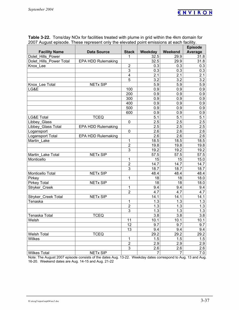
September 2004
H:\etcog3\report\sept04\sec3.doc 3-37
Table 3-22. Tons/day NOx for facilities treated with plume in grid within the 4km domain for 2007 August episode. These represent only the elevated point emissions at each facility.
Facility Name Data Source Stack Weekday Weekend Episode Average
Dolet_Hills_Power 1 32.5 29.9 31.8Dolet_Hills_Power Total EPA HDD Rulemaking 32.5 29.9 31.8Knox_Lee 2 0.3 0.3 0.3 3 0.3 0.3 0.3 4 2.1 2.1 2.1 5 3.2 3.2 3.2Knox_Lee Total NETx SIP 5.9 5.9 5.9LG&E 100 0.9 0.9 0.9 200 0.9 0.9 0.9 300 0.9 0.9 0.9 400 0.9 0.9 0.9 500 0.9 0.9 0.9 600 0.9 0.9 0.9LG&E Total TCEQ 5.1 5.1 5.1Libbey_Glass 0 2.5 2.5 2.5Libbey_Glass Total EPA HDD Rulemaking 2.5 2.5 2.5Logansport 0 2.6 2.6 2.6Logansport Total EPA HDD Rulemaking 2.6 2.6 2.6Martin_Lake 1 18.5 18.5 18.5 2 19.8 19.8 19.8 3 19.2 19.2 19.2Martin_Lake Total NETx SIP 57.5 57.5 57.5Monticello 1 15 15 15.0 2 14.7 14.7 14.7 3 18.7 18.7 18.7Monticello Total NETx SIP 48.4 48.4 48.4Pirkey 1 18 18 18.0Pirkey Total NETx SIP 18 18 18.0Stryker_Creek 1 9.4 9.4 9.4 2 4.7 4.7 4.7Stryker_Creek Total NETx SIP 14.1 14.1 14.1Tenaska 1 1.3 1.3 1.3 2 1.3 1.3 1.3 3 1.3 1.3 1.3Tenaska Total TCEQ 3.8 3.8 3.8Welsh 11 10.1 10.1 10.1 12 9.7 9.7 9.7 13 9.4 9.4 9.4Welsh Total TCEQ 29.2 29.2 29.2Wilkes 1 1.5 1.5 1.5 2 2.9 2.9 2.9 3 2.6 2.6 2.6Wilkes Total NETx SIP 7 7 7.0Note: The August 2007 episode consists of the dates Aug. 13-22. Weekday dates correspond to Aug. 13 and Aug. 16-20. Weekend dates are Aug. 14-15 and Aug. 21-22

September 2004
H:\etcog3\report\sept04\sec3.doc 3-38
Table 3-23. Eastman Chemical Co. total elevated and surface NOx tpd for average August 2007 episode day. The 'other' represents over a hundred individual stacks.
Cogen Unit
Stack 1 Cogen Unit
Stack 2 Other Elevated Other Surface Total NOx 1.05 1.05 6.5 1.1 9.7 VOC 0.0 0.0 1.0 11.9 12.9
Note: The cogen unit emissions are not actually Eastman Chemical Co. emissions, but are included in this table because Eastman agreed to offset the cogen emissions as part of their overall NOx reduction commitment. Table 3-24. ‘New’ point sources in Northeast Texas. Sources in the 2007 modeling which were not present in the 1999 base year modeling.
Facility Name County NOx Entergy Power Ventures Harrison 0.9 LG&E Power Anderson 5.1 Tenaska Gateway Rusk 3.8
Figure 3-3. 2007 average episode day NOx for the facilities in Table 3-22. These represent elevated sources for all facilities with the exception of Texas Eastman Chemical Co. which represents the total NOx from Table 3-23.

September 2004
H:\etcog3\report\sept04\sec3.doc 3-39
Table 3-25. Texas gridded 2007 episode day emissions by major source type.
Episode Day Area
Off- road
On- road EGUs
Other Points
Off- Shore
Ship- ping
Total Anthro-pogenic
Bio-genic Total
Tons NOx Friday, August 13 712 853 837 745 1314 549 40 5050 1100 6150Saturday, August 14 693 843 623 745 1309 549 40 4802 1082 5884Sunday, August 15 675 781 501 745 1309 549 40 4601 1105 5706Monday, August 16 712 853 892 745 1314 549 40 5105 1082 6187Tuesday, August 17 712 853 898 745 1314 549 40 5111 1040 6151Wednesday, August 18 712 853 852 745 1314 549 40 5065 1078 6143Thursday, August 19 712 853 849 745 1314 549 40 5062 1068 6129Friday, August 20 712 853 860 745 1314 549 40 5073 1052 6125Saturday, August 21 693 843 629 745 1309 549 40 4808 1053 5861Sunday, August 22 675 781 490 745 1309 549 40 4589 1010 5599Tons VOC Friday, August 13 1967 377 564 23 673 189 1 3794 22087 25881Saturday, August 14 1554 704 494 23 644 189 1 3610 20527 24137Sunday, August 15 1324 696 429 23 644 189 1 3305 20445 23750Monday, August 16 1967 377 503 23 673 189 1 3732 19998 23730Tuesday, August 17 1967 377 513 23 673 189 1 3743 19290 23033Wednesday, August 18 1967 377 448 23 673 189 1 3677 20752 24430Thursday, August 19 1967 377 447 23 673 189 1 3677 21745 25421Friday, August 20 1967 377 576 23 673 189 1 3805 20788 24593Saturday, August 21 1554 704 488 23 644 189 1 3604 19565 23168Sunday, August 22 1324 696 417 23 644 189 1 3293 18023 21317Tons CO Friday, August 13 1034 6282 7137 208 1073 126 6 15866 2270 18136Saturday, August 14 889 9210 6486 208 1063 126 6 17988 2159 20146Sunday, August 15 746 9093 5729 208 1063 126 6 16971 2128 19099Monday, August 16 1034 6282 6317 208 1073 126 6 15046 2078 17124Tuesday, August 17 1034 6282 6488 208 1073 126 6 15217 2005 17222Wednesday, August 18 1034 6282 5791 208 1073 126 6 14520 2136 16656Thursday, August 19 1034 6282 5658 208 1073 126 6 14386 2212 16599Friday, August 20 1034 6282 7065 208 1073 126 6 15794 2127 17922Saturday, August 21 889 9210 6407 208 1063 126 6 17909 2045 19954Sunday, August 22 746 9093 5717 208 1063 126 6 16960 1963 18923
Table 3-26. Summary of August 2007 gridded emissions by major source type for states other than Texas.
Area Off-road On-road Point Anthropogenic
State Weekday Sat Sun
Week day Sat Sun
Week day Sat Sun
Weekday Sat Sun
Total Weekday
Total Sat
Total Sun
NOx Alabama 163 150 144 209 212 196 316 237 237 457 437 437 1144 1036 1014Arkansas 128 118 113 145 147 137 193 145 145 237 223 223 703 633 618Florida 6 5 5 59 67 63 86 64 64 128 122 122 278 259 254Georgia 58 54 52 197 181 158 475 357 357 255 240 240 985 832 807Illinois 13 12 12 204 204 197 145 109 109 274 263 263 637 588 581Indiana 32 30 29 140 134 124 159 119 119 260 242 242 591 525 514Kansas 242 222 213 326 319 306 173 130 130 553 527 527 1294 1198 1175Kentucky 259 239 229 252 254 242 304 228 228 357 335 335 1172 1056 1033Louisiana 355 327 312 633 646 631 263 197 197 1058 1037 1037 2309 2207 2177Mississippi 157 144 138 168 170 159 220 165 165 429 412 412 974 891 874Missouri 38 36 34 318 332 312 407 306 306 240 226 226 1004 899 877Nebraska 4 4 4 46 45 45 12 9 9 45 43 43 107 101 100North Carolina 1 1 1 4 3 3 13 10 10 7 7 7 25 21 21Ohio 24 22 21 61 56 49 91 69 69 188 175 175 364 321 313Oklahoma 103 95 91 158 163 153 269 202 202 647 619 619 1177 1078 1064South Carolina 0 0 0 0 0 0 3 2 2 0 0 0 3 3 3

September 2004
H:\etcog3\report\sept04\sec3.doc 3-40
Area Off-road On-road Point Anthropogenic
State Weekday Sat Sun
Week day Sat Sun
Week day Sat Sun
Weekday Sat Sun
Total Weekday
Total Sat
Total Sun
Tennessee 69 65 63 448 449 430 387 290 290 320 307 307 1223 1111 1090Virginia 1 1 1 3 3 2 6 5 5 0 0 0 10 8 8West Virginia 3 3 3 42 42 41 10 8 8 52 48 48 107 101 100Grand Total 1655 1527 1463 3413 3427 3246 3533 2650 2650 5509 5263 5263 14110 12866 12622VOC Alabama 387 387 387 137 311 309 226 169 169 167 167 167 918 1035 1032Arkansas 350 350 350 82 179 177 119 89 89 35 35 35 587 653 652Florida 119 119 119 77 191 190 57 43 43 13 13 13 266 365 365Georgia 476 476 476 149 217 213 291 218 218 78 78 78 995 990 986Illinois 178 178 178 60 99 98 82 61 61 117 117 117 437 455 454Indiana 238 238 238 48 80 78 95 71 71 39 39 39 420 427 426Kansas 365 364 364 77 114 112 106 80 80 40 40 40 588 598 596Kentucky 378 378 377 94 196 195 181 135 135 180 180 180 832 889 887Louisiana 323 322 322 153 349 347 159 120 120 242 241 241 876 1032 1030Mississippi 371 371 371 91 212 210 129 97 97 151 151 151 742 831 829Missouri 421 421 421 173 383 380 249 187 187 158 157 157 1001 1148 1145Nebraska 45 45 45 8 11 10 7 5 5 3 3 3 62 63 63North Carolina 17 17 17 5 10 10 7 5 5 3 3 3 33 36 36Ohio 131 131 131 37 46 45 59 45 45 29 29 29 256 250 249Oklahoma 290 290 290 86 176 174 185 139 139 97 96 96 657 700 699South Carolina 2 2 2 0 0 0 2 1 1 0 0 0 4 3 3Tennessee 664 664 664 137 280 277 238 178 178 193 193 193 1231 1315 1312Virginia 8 8 8 1 1 1 4 3 3 1 1 1 13 12 12West Virginia 15 15 15 6 11 11 6 5 5 7 7 7 34 38 38Grand Total 4778 4776 4775 1421 2866 2838 2202 1651 1651 1552 1549 1549 9953 10843 10813CO Alabama 181 179 177 1275 2086 2053 2268 1701 1701 613 611 611 4338 4577 4544Arkansas 100 98 98 865 1409 1388 1290 968 968 330 329 329 2585 2804 2782Florida 5 5 5 438 830 823 584 438 438 40 40 40 1068 1314 1306Georgia 171 170 170 2022 2805 2758 3244 2433 2433 230 228 228 5667 5637 5589Illinois 22 22 22 788 1096 1081 959 719 719 62 61 61 1832 1898 1884Indiana 40 39 39 817 1097 1076 1081 811 811 265 263 263 2203 2210 2189Kansas 140 137 135 1208 1634 1608 1197 897 897 241 238 238 2785 2906 2878Kentucky 175 171 170 1063 1731 1705 1978 1484 1484 235 232 232 3451 3618 3591Louisiana 117 113 110 1398 2445 2416 1753 1315 1315 2435 2431 2431 5702 6303 6272Mississippi 128 126 125 749 1252 1231 1246 934 934 363 360 360 2486 2673 2650Missouri 157 156 156 2450 3802 3758 2735 2051 2051 317 315 315 5658 6324 6280Nebraska 14 14 14 108 147 145 74 55 55 7 7 7 203 223 222North Carolina 11 11 11 48 68 67 83 62 62 10 10 10 152 152 151Ohio 54 54 54 904 1107 1092 637 478 478 100 99 99 1695 1737 1722Oklahoma 77 75 75 1121 1742 1723 1849 1387 1387 679 674 674 3725 3878 3859South Carolina 1 1 1 1 1 1 19 15 15 0 0 0 21 16 16Tennessee 250 248 247 1656 2610 2569 2588 1941 1941 299 298 298 4793 5097 5056Virginia 5 5 5 13 18 17 38 28 28 0 0 0 56 52 51West Virginia 5 5 5 60 93 91 71 53 53 13 13 13 149 164 162Grand Total 1653 1631 1620 16984 25974 25605 23695 17771 17771 6240 6209 6209 48571 51584 51204

September 2004
H:\etcog3\report\sept04\sec3.doc 3-41
Table 3-27. Gridded biogenic emissions for states other than Texas. 13-Aug 14-Aug 15-Aug 16-Aug 17-Aug 18-Aug 19-Aug 20-Aug 21-Aug 22-AugNOx (tpd) Alabama 78 68 64 70 74 77 74 68 67 68Arkansas 128 96 94 109 126 134 129 103 102 112Florida 11 10 9 9 10 10 10 9 9 9Georgia 51 49 45 47 47 49 48 44 45 46Illinois 338 271 282 343 385 334 303 292 299 333Indiana 158 112 121 145 164 144 128 120 130 141Kansas 444 497 613 689 645 574 494 472 549 549Kentucky 154 108 113 139 160 149 143 118 122 134Louisiana 111 102 91 98 106 112 116 106 101 103Mississippi 133 108 99 113 127 133 137 116 110 118Missouri 245 215 242 300 314 294 250 235 250 270Nebraska 148 176 221 226 211 192 170 175 194 192North Carolina 2 1 1 1 2 1 2 1 1 1Ohio 22 17 18 20 25 20 19 17 18 20Oklahoma 196 195 220 238 232 233 202 187 208 216South Carolina 0 0 0 0 0 0 0 0 0 0Tennessee 122 86 87 107 120 122 118 93 94 103Virginia 1 1 0 1 1 1 1 0 0 1West Virginia 0 0 0 0 1 0 0 0 0 0NOX Totals 2342 2112 2322 2656 2750 2581 2342 2158 2301 2415VOC (tpd) Alabama 14097 11687 10261 11937 12969 14092 12878 11027 10796 10584Arkansas 11291 7772 7543 9151 11323 12454 11394 8109 8074 9278Florida 2772 2287 2158 2335 2424 2413 2501 2227 2391 2268Georgia 5614 5244 4760 5001 5229 5973 5539 4163 4471 4451Illinois 1692 982 1211 1758 1987 1250 1215 1236 1343 1558Indiana 1395 554 823 1163 1421 999 837 747 910 1067Kansas 973 1127 1674 2129 1944 1678 1204 1015 1365 1136Kentucky 3596 1383 1808 2922 3641 2991 2727 1654 2109 2645Louisiana 9282 8317 6817 7615 8392 8981 9574 8468 7649 7784Mississippi 14325 10911 9068 11206 12666 13599 13921 11249 10355 11261Missouri 7786 5601 7350 10521 11716 10253 7380 6513 7538 8222Nebraska 143 225 345 363 330 276 212 225 266 218North Carolina 602 497 414 512 568 547 565 367 356 388Ohio 210 86 113 170 234 163 122 110 133 423Oklahoma 6505 5351 5630 6046 6717 7195 6392 4891 5089 5953South Carolina 105 102 83 90 95 111 107 70 72 83Tennessee 8016 3911 4390 6723 7714 7522 7131 4132 4768 5342Virginia 98 62 46 91 109 91 82 46 50 71West Virginia 88 37 38 68 93 66 59 36 47 103VOC Totals 88590 66134 64531 79801 89572 90652 83840 66284 67781 72836CO (tpd) Alabama 1349 1141 1014 1143 1231 1328 1223 1092 1068 1073Arkansas 1030 752 705 834 1019 1132 1030 776 764 859Florida 354 313 282 301 309 313 312 291 300 295Georgia 517 457 411 433 451 495 474 381 391 401Illinois 166 108 117 155 180 149 136 123 127 146Indiana 145 82 93 123 147 118 101 90 101 118Kansas 136 149 205 257 241 210 155 143 176 173Kentucky 344 196 194 276 337 288 267 195 212 263Louisiana 953 882 722 791 872 934 1002 885 810 815Mississippi 1302 1022 847 1011 1142 1232 1246 1036 959 1037Missouri 610 470 551 742 842 801 594 524 574 630
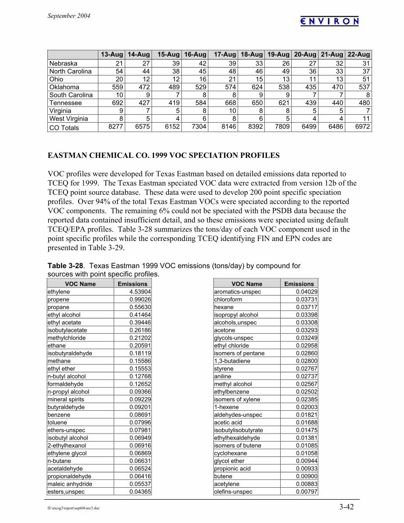
September 2004
H:\etcog3\report\sept04\sec3.doc 3-42
13-Aug 14-Aug 15-Aug 16-Aug 17-Aug 18-Aug 19-Aug 20-Aug 21-Aug 22-AugNebraska 21 27 39 42 39 33 26 27 32 31North Carolina 54 44 38 45 48 46 49 36 33 37Ohio 20 12 12 16 21 15 13 11 13 51Oklahoma 559 472 489 529 574 624 538 435 470 537South Carolina 10 9 7 8 8 9 9 7 7 8Tennessee 692 427 419 584 668 650 621 439 440 480Virginia 9 7 5 8 10 8 8 5 5 7West Virginia 8 5 4 6 8 6 5 4 4 11CO Totals 8277 6575 6152 7304 8146 8392 7809 6499 6486 6972 EASTMAN CHEMICAL CO. 1999 VOC SPECIATION PROFILES VOC profiles were developed for Texas Eastman based on detailed emissions data reported to TCEQ for 1999. The Texas Eastman speciated VOC data were extracted from version 12b of the TCEQ point source database. These data were used to develop 200 point specific speciation profiles. Over 94% of the total Texas Eastman VOCs were speciated according to the reported VOC components. The remaining 6% could not be speciated with the PSDB data because the reported data contained insufficient detail, and so these emissions were speciated using default TCEQ/EPA profiles. Table 3-28 summarizes the tons/day of each VOC component used in the point specific profiles while the corresponding TCEQ identifying FIN and EPN codes are presented in Table 3-29. Table 3-28. Texas Eastman 1999 VOC emissions (tons/day) by compound for sources with point specific profiles.
VOC Name Emissions ethylene 4.53904 propene 0.99026 propane 0.55630 ethyl alcohol 0.41464 ethyl acetate 0.39446 isobutylacetate 0.26186 methylchloride 0.21202 ethane 0.20591 isobutyraldehyde 0.18119 methane 0.15586 ethyl ether 0.15553 n-butyl alcohol 0.12768 formaldehyde 0.12652 n-propyl alcohol 0.09366 mineral spirits 0.09229 butyraldehyde 0.09201 benzene 0.08691 toluene 0.07996 ethers-unspec 0.07981 isobutyl alcohol 0.06949 2-ethylhexanol 0.06916 ethylene glycol 0.06869 n-butane 0.06631 acetaldehyde 0.06524 propionaldehyde 0.06416 maleic anhydride 0.05537 esters,unspec 0.04365
VOC Name Emissions aromatics-unspec 0.04029 chloroform 0.03731 hexane 0.03717 isopropyl alcohol 0.03398 alcohols,unspec 0.03308 acetone 0.03293 glycols-unspec 0.03249 ethyl chloride 0.02958 isomers of pentane 0.02860 1,3-butadiene 0.02800 styrene 0.02767 aniline 0.02737 methyl alcohol 0.02567 ethylbenzene 0.02502 isomers of xylene 0.02385 1-hexene 0.02003 aldehydes-unspec 0.01821 acetic acid 0.01688 isobutylisobutyrate 0.01475 ethylhexaldehyde 0.01381 isomers of butene 0.01085 cyclohexane 0.01058 glycol ether 0.00944 propionic acid 0.00933 butene 0.00900 acetylene 0.00883 olefins-unspec 0.00797

September 2004
H:\etcog3\report\sept04\sec3.doc 3-43
VOC Name Emissions isobutane 0.00744 heptane 0.00678 methylacrylate 0.00672 acrylonitrile 0.00628 isopentane 0.00609 napthalene 0.00524 methylethyl ketone 0.00426 tetrahydrofuran 0.00355 ethylene oxide 0.00324 isomers of hexane 0.00280 methylisobutyl keto 0.00262 4-methylaniline 0.00213 t-butyl alcohol 0.00210 butylacrylate 0.00190 o-xylene 0.00144 sec-butyl alcohol 0.00131 vinyl acetate 0.00129 crotonaldehyde 0.00074 n-butylacetate 0.00065 carbon tetrachlorid 0.00052 n-propylacetate 0.00040 chlorobenzene 0.00038
VOC Name Emissions 3-methylpentane 0.00031 hexadiene 0.00028 octane 0.00024 methylcyclopentane 0.00022 formic acid 0.00015 acrylic acid 0.00015 naphtha 0.00015 chlorinated hydrocar 0.00007 cyclopentane 0.00005 methylformate 0.00004 trans-2-butene 0.00003 ethylene dichloride 0.00003 ethylene dibromide 0.00003 methyl acrylic acid 0.00003 n-hexanol 0.00003 ketones-unspec 0.00003 nonane 0.00002 n-pentane 0.00001 ethyl acrylate 0.00001 acetonitrile 0.00001
Table 3-29. Texas Eastman point sources (EPN/FIN) for which facility specific speciation profiles were developed and total VOC emissions by point.
FIN EPN Total VOC (tons/day)
EB025T51 025T62 0.00742EB025T58 025T62 0.01445EB025WW1 F025WW1 0.01006EB093FG1 F093FG1 0.00848EB093T703 093T704 0.04689EB106FG1 F106FG1 0.00564EB108FG2 F108FG2 0.06323EB108KT7 108KT7 0.01713EB108T521 042FL1 0.02199EP008FG1 F008FG1 0.56191EP008FG2 F008FG2 0.12979EP008T71 008T71 0.00838EP009T14 116FL2H 0.02048EP034D203 034D203 0.17016EP035D203 035D203 0.11751EP036FG1 F036FG1 0.02194EP036U1 036U1 0.01343EP037FG1 F037FG1 0.01840EP037GA1 037GA1 0.00572EP037U501 037U501 0.05498EP038FG1 F038FG1 0.00695EP038FG2 F038FG2 0.00581OL007FG1 F007FG1 0.20317OL007VS1 116FL2H 0.04764OL014FG2 F014FG2 0.01033OL014FG3 F014FG3 0.00602OL032FG1 F032FG1 0.42642
FIN EPN Total VOC (tons/day)
OL032GA1 032GA1 0.01572OL032VS1 233FL1 0.07251OL033FG1 F033FG1 0.65063OL033GA1 033GA1 0.01280OL033VS1 170FL1 0.07484OL041FG1 F041FG1 0.04594OL041FG2 F041FG2 0.00776OL042FL2 042FL2 0.00630OL043FG1 F043FG1 0.56196OL043VS1 042FL1 0.06909OL170FL2 170FL2 0.00772OL225B1A 225B1A 0.00878OL225B1B 225B1B 0.00878OL226FG1 F226FG1 0.91296OL226VS1 225FL1 0.00570OL229CT7 F136CT7 0.02262OL229H1 229H1 0.00515OL229H2 229H2 0.00515OL229H3 229H3 0.00515OL229H4 229H4 0.00515OL229WW1 229WW1 0.01420OLF041FG3 F041FG3 0.00665OX010FG3 F010FG3 0.01034OX010T220 030B11 0.00563OX011FG3 F011FG3 0.02355OX015FG1 F015FG1 0.13892OX015FG2 F015FG2 0.28606

September 2004
H:\etcog3\report\sept04\sec3.doc 3-44
FIN EPN Total VOC (tons/day)
OX015R502 015E508 0.08448OX015R504 015E550 0.13305OX015R507 015E569 0.08448OX015T507 015T507 0.02220OX015T508 015VS1 0.01798OX015T524 015VS1 0.01562OX015T535 015E505 0.01018OX015T94 015T96 0.00527OX016FG1 F016FG1 0.02131OX016FG2 F016FG2 0.02131OX016FG3 F016FG3 0.01126OX016T560 016E573 0.01018OX016VS4 016CU1 0.00616OX050T422 050T422 0.00577OX053FG1 F053FG1 0.23133OX053FG2 F053FG2 0.09875OX061FG1 F061FG1 0.03071OX061H1 061CD6 0.00566OX061H1 061CD7 0.00566OX061H5 061CD12 0.00575OX061H5 061CD17 0.01579OX061H7 061CD14 0.01632OX061H7 061CD61 0.01632OX062C16 062C16 0.01287OX062C17 062C17 0.01284OX062C19 062C19 0.01297OX062C20 062C20 0.01273OX062C22 062C22 0.01642OX062C7 062C7 0.01204OX062C9 062C9 0.01073OX062FG1 F062FG1 0.03317OX062H11A 062CD18A 0.00839OX062H11A 062CD18B 0.00839OX062H11A 062CD18C 0.00839OX062H11B 062CD18A 0.00839OX062H11B 062CD18B 0.00839OX062H11B 062CD18C 0.00839OX062H13A 062CD26 0.01529OX062H13A 062CD28 0.01529OX062H13B 062CD26 0.01529OX062H13B 062CD28 0.01529OX062H17 062CD32 0.02950OXF010FG2 F010FG2 0.08329OXO10FG1 F010FG1 0.07762PE012C1C 012C1CE 0.00509PE012DM4B5 012DM4B5 0.00827PE012FG1 F012FG1 0.17988PE012FG4 F012FG4 0.39147PE012FG5 F012FG5 0.47169PE012FG6 F012FG6 0.01997PE012FG8 063CU1 0.00877PE012FG8 F012FG8 0.19044PE012P12BD 012P12BD 0.00821PE012S34G 012S34G 0.01643PE012S34P 012S34P 0.00821PE012S34R 012S34R 0.00822
FIN EPN Total VOC (tons/day)
PE012S34Y 012S34Y 0.00821PE012S78 012S78 0.03603PE012S79 012S79 0.03603PE012S80 116FL2H 0.01576PE012STD 012STD 0.01216PE012STE 012STE 0.00520PE013C1F 013C1FE 0.00737PE013C1G 013C1GE 0.01002PE013C7A 013C7AE 0.01248PE013C7B 013C7BE 0.01248PE013D310 013D310 0.01140PE013D311 013D311 0.01140PE013D312 013D312 0.01140PE013D313 013D313 0.01140PE013D340 013D340 0.01842PE013D341 013D341 0.01842PE013D342 013D342 0.01842PE013D343 013D343 0.01842PE013D344 013D344 0.01842PE013D345 013D345 0.01842PE013DM4B6 013DM4B6 0.00827PE013DM4B7 013DM4B7 0.03033PE013DMR1 013DMR1 0.01745PE013FG1 F013FG1 0.43451PE013S34H 013S34H 0.00821PE063C5A 063C5AE 0.00908PE063C5B 063C5BE 0.00908PE065D614 065D614 0.00777PE065D615 065D615 0.00777PE065D616 065D616 0.00777PE065D617 065D617 0.00777PE065D618 065D618 0.00777PE066FG1 F066FG1 0.08703PE066FG2 F066FG2 0.02397PE066FG3 F066FG3 0.01744PE137VS1 137VS1 0.08770PE143FG1 F143FG1 0.17180PE146FG1 F146FG1 0.00776PE224T01 224T01 0.00733PE224VS1 145FL1 0.01083PE252EX1 F045CT5 0.00797PE252F710 252BH710 0.00571PE252FG1 F252FG1 0.07270PE252VS1 085FL1 0.02619PE256FG1 F256FG1 0.01005PP028FG1 F028FG1 0.16774PP028T331 054FL2 0.00897PP028VS1 054FL2 0.00749PP054FL2 054FL2 0.01716RD005AV2 F005AV2 0.00659RD005FG6 F005FG6 0.12189RD005FG7 F005FG7 0.02959RD005S3425 128FL1 0.00773RD059FG1 F059FG1 0.01389RDF066FG4 F066FG4 0.00938SD008LR1 008LR1 0.02006
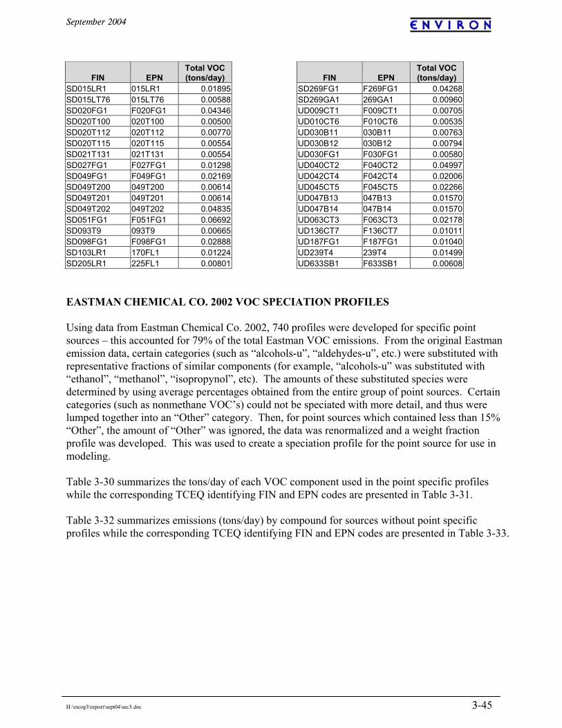
September 2004
H:\etcog3\report\sept04\sec3.doc 3-45
FIN EPN Total VOC (tons/day)
SD015LR1 015LR1 0.01895SD015LT76 015LT76 0.00588SD020FG1 F020FG1 0.04346SD020T100 020T100 0.00500SD020T112 020T112 0.00770SD020T115 020T115 0.00554SD021T131 021T131 0.00554SD027FG1 F027FG1 0.01298SD049FG1 F049FG1 0.02169SD049T200 049T200 0.00614SD049T201 049T201 0.00614SD049T202 049T202 0.04835SD051FG1 F051FG1 0.06692SD093T9 093T9 0.00665SD098FG1 F098FG1 0.02888SD103LR1 170FL1 0.01224SD205LR1 225FL1 0.00801
FIN EPN Total VOC (tons/day)
SD269FG1 F269FG1 0.04268SD269GA1 269GA1 0.00960UD009CT1 F009CT1 0.00705UD010CT6 F010CT6 0.00535UD030B11 030B11 0.00763UD030B12 030B12 0.00794UD030FG1 F030FG1 0.00580UD040CT2 F040CT2 0.04997UD042CT4 F042CT4 0.02006UD045CT5 F045CT5 0.02266UD047B13 047B13 0.01570UD047B14 047B14 0.01570UD063CT3 F063CT3 0.02178UD136CT7 F136CT7 0.01011UD187FG1 F187FG1 0.01040UD239T4 239T4 0.01499UD633SB1 F633SB1 0.00608
EASTMAN CHEMICAL CO. 2002 VOC SPECIATION PROFILES Using data from Eastman Chemical Co. 2002, 740 profiles were developed for specific point sources – this accounted for 79% of the total Eastman VOC emissions. From the original Eastman emission data, certain categories (such as “alcohols-u”, “aldehydes-u”, etc.) were substituted with representative fractions of similar components (for example, “alcohols-u” was substituted with “ethanol”, “methanol”, “isopropynol”, etc). The amounts of these substituted species were determined by using average percentages obtained from the entire group of point sources. Certain categories (such as nonmethane VOC’s) could not be speciated with more detail, and thus were lumped together into an “Other” category. Then, for point sources which contained less than 15% “Other”, the amount of “Other” was ignored, the data was renormalized and a weight fraction profile was developed. This was used to create a speciation profile for the point source for use in modeling. Table 3-30 summarizes the tons/day of each VOC component used in the point specific profiles while the corresponding TCEQ identifying FIN and EPN codes are presented in Table 3-31. Table 3-32 summarizes emissions (tons/day) by compound for sources without point specific profiles while the corresponding TCEQ identifying FIN and EPN codes are presented in Table 3-33.
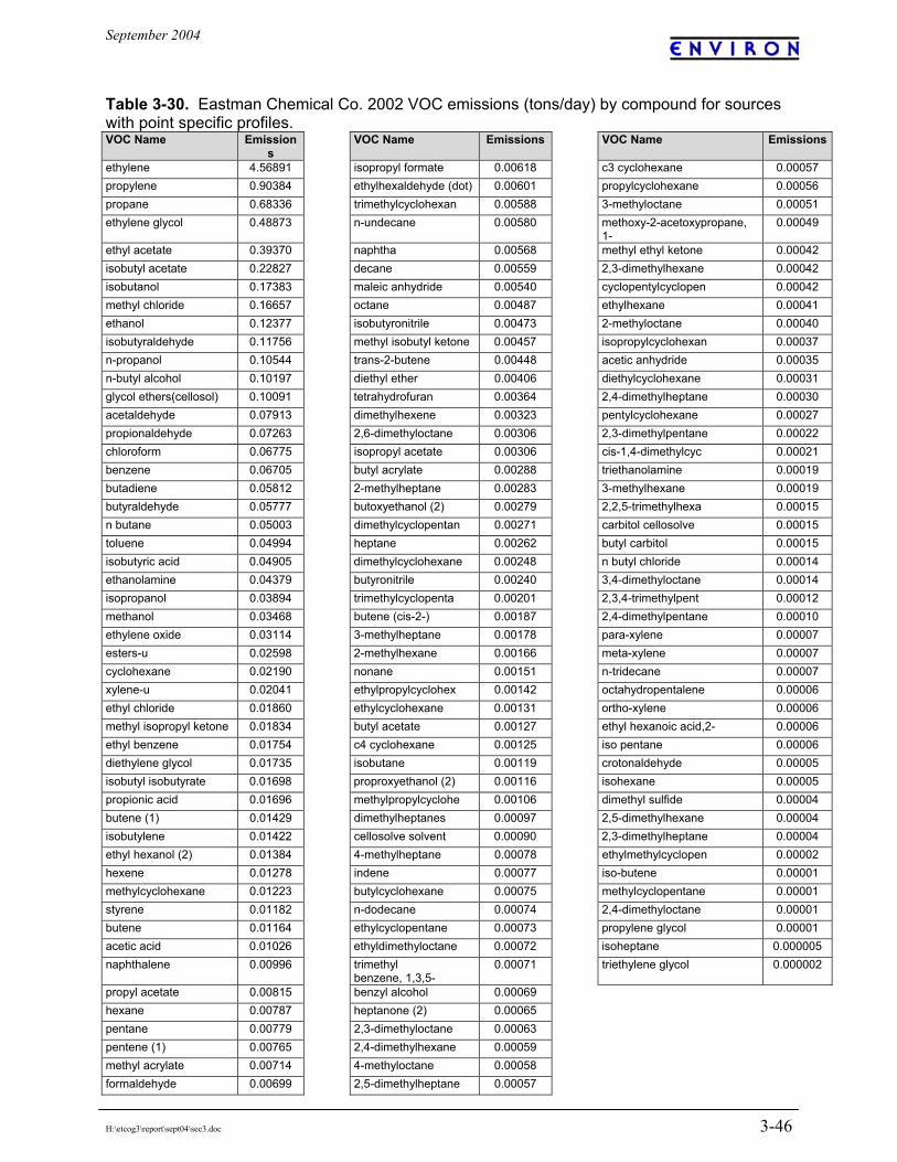
September 2004
H:\etcog3\report\sept04\sec3.doc 3-46
Table 3-30. Eastman Chemical Co. 2002 VOC emissions (tons/day) by compound for sources with point specific profiles. VOC Name Emission
s VOC Name Emissions VOC Name Emissions
ethylene 4.56891 isopropyl formate 0.00618 c3 cyclohexane 0.00057 propylene 0.90384 ethylhexaldehyde (dot) 0.00601 propylcyclohexane 0.00056 propane 0.68336 trimethylcyclohexan 0.00588 3-methyloctane 0.00051 ethylene glycol 0.48873 n-undecane 0.00580 methoxy-2-acetoxypropane,
1- 0.00049
ethyl acetate 0.39370 naphtha 0.00568 methyl ethyl ketone 0.00042 isobutyl acetate 0.22827 decane 0.00559 2,3-dimethylhexane 0.00042 isobutanol 0.17383 maleic anhydride 0.00540 cyclopentylcyclopen 0.00042 methyl chloride 0.16657 octane 0.00487 ethylhexane 0.00041 ethanol 0.12377 isobutyronitrile 0.00473 2-methyloctane 0.00040 isobutyraldehyde 0.11756 methyl isobutyl ketone 0.00457 isopropylcyclohexan 0.00037 n-propanol 0.10544 trans-2-butene 0.00448 acetic anhydride 0.00035 n-butyl alcohol 0.10197 diethyl ether 0.00406 diethylcyclohexane 0.00031 glycol ethers(cellosol) 0.10091 tetrahydrofuran 0.00364 2,4-dimethylheptane 0.00030 acetaldehyde 0.07913 dimethylhexene 0.00323 pentylcyclohexane 0.00027 propionaldehyde 0.07263 2,6-dimethyloctane 0.00306 2,3-dimethylpentane 0.00022 chloroform 0.06775 isopropyl acetate 0.00306 cis-1,4-dimethylcyc 0.00021 benzene 0.06705 butyl acrylate 0.00288 triethanolamine 0.00019 butadiene 0.05812 2-methylheptane 0.00283 3-methylhexane 0.00019 butyraldehyde 0.05777 butoxyethanol (2) 0.00279 2,2,5-trimethylhexa 0.00015 n butane 0.05003 dimethylcyclopentan 0.00271 carbitol cellosolve 0.00015 toluene 0.04994 heptane 0.00262 butyl carbitol 0.00015 isobutyric acid 0.04905 dimethylcyclohexane 0.00248 n butyl chloride 0.00014 ethanolamine 0.04379 butyronitrile 0.00240 3,4-dimethyloctane 0.00014 isopropanol 0.03894 trimethylcyclopenta 0.00201 2,3,4-trimethylpent 0.00012 methanol 0.03468 butene (cis-2-) 0.00187 2,4-dimethylpentane 0.00010 ethylene oxide 0.03114 3-methylheptane 0.00178 para-xylene 0.00007 esters-u 0.02598 2-methylhexane 0.00166 meta-xylene 0.00007 cyclohexane 0.02190 nonane 0.00151 n-tridecane 0.00007 xylene-u 0.02041 ethylpropylcyclohex 0.00142 octahydropentalene 0.00006 ethyl chloride 0.01860 ethylcyclohexane 0.00131 ortho-xylene 0.00006 methyl isopropyl ketone 0.01834 butyl acetate 0.00127 ethyl hexanoic acid,2- 0.00006 ethyl benzene 0.01754 c4 cyclohexane 0.00125 iso pentane 0.00006 diethylene glycol 0.01735 isobutane 0.00119 crotonaldehyde 0.00005 isobutyl isobutyrate 0.01698 proproxyethanol (2) 0.00116 isohexane 0.00005 propionic acid 0.01696 methylpropylcyclohe 0.00106 dimethyl sulfide 0.00004 butene (1) 0.01429 dimethylheptanes 0.00097 2,5-dimethylhexane 0.00004 isobutylene 0.01422 cellosolve solvent 0.00090 2,3-dimethylheptane 0.00004 ethyl hexanol (2) 0.01384 4-methylheptane 0.00078 ethylmethylcyclopen 0.00002 hexene 0.01278 indene 0.00077 iso-butene 0.00001 methylcyclohexane 0.01223 butylcyclohexane 0.00075 methylcyclopentane 0.00001 styrene 0.01182 n-dodecane 0.00074 2,4-dimethyloctane 0.00001 butene 0.01164 ethylcyclopentane 0.00073 propylene glycol 0.00001 acetic acid 0.01026 ethyldimethyloctane 0.00072 isoheptane 0.000005 naphthalene 0.00996 trimethyl
benzene, 1,3,5- 0.00071 triethylene glycol 0.000002
propyl acetate 0.00815 benzyl alcohol 0.00069 hexane 0.00787 heptanone (2) 0.00065 pentane 0.00779 2,3-dimethyloctane 0.00063 pentene (1) 0.00765 2,4-dimethylhexane 0.00059 methyl acrylate 0.00714 4-methyloctane 0.00058 formaldehyde 0.00699 2,5-dimethylheptane 0.00057

September 2004
H:\etcog3\report\sept04\sec3.doc 3-47
VOC Name Emissions
VOC Name Emissions VOC Name Emissions
2-methyldecane 0.00652 ethylmethylcyclohex 0.00057
Table 3-31. Eastman Chemical Co. point sources (EPN/FIN) for which facility specific speciation profiles were developed and total VOC emissions by point - (181 out of 740 sources listed, these contribute 98% of the emissions for the entire group).
FIN EPN Total VOC (tons/day) FIN EPN
Total VOC (tons/day)
OL226FG1 F226FG1 1.286880548 EP034D203 034D203 0.02304OL032FG1 F032FG1 0.772957808 SD008SP45 008LT45 0.023021644OL033FG1 F033FG1 0.745787945 SD049FG1 F049FG1 0.022164384OL043FG1 F043FG1 0.557879178 OL042FL2 042FL2 0.020353151PE013FG3 F013FG3 0.407310411 PE012FG6 F012FG6 0.020075616PE013FG1 F013FG1 0.385220548 OX015T524 015VS1 0.019608219PE012FG4 F012FG4 0.336139726 OX016FG1 F016FG1 0.019506849EP037U501 037U501 0.317808219 PE013D341 013D341 0.01735863OX015FG2 F015FG2 0.315780822 PE013D342 013D342 0.01735863OL007FG1 F007FG1 0.240781918 PE013D343 013D343 0.01735863EP035D203 035D203 0.22162 PE013D344 013D344 0.01735863OX010FG3 F010FG3 0.204381096 PE013D345 013D345 0.01735863PE012FG8 F012FG8 0.190936438 SD015LR1 015LR1 0.01729589PE143FG1 F143FG1 0.17430137 PE012S34Y 012S34Y 0.016465753PE012FG1 F012FG1 0.153418904 EP036D4 036D4 0.01545RD005FG6 F005FG6 0.150153151 EB025T51 025T62 0.01542OX015R504 015E550 0.133452055 PE252VS2 146FL2 0.015176438SD052LR1 052LR1 0.133352329 OX016S300 016CU2 0.013673973OX015FG1 F015FG1 0.120164384 EP008FG1 F008FG1 0.01334EP036U1 036U1 0.11918 PE013DMR1 013DMR1 0.013103014SD051FG2 F051FG2 0.094383288 SD027FG1 F027FG1 0.01301726PP028FG1 F028FG1 0.092699452 SD103LR2 170FL1 0.012814247PE137VS1 137VS1 0.090027397 RD005FG13 005FG13 0.012485205OX015R502 015E508 0.084712329 UD119TK2 119TK2 0.011464384OX015R507 015E569 0.084712329 UD119TK3 119TK3 0.011464384OX010FG1 F010FG1 0.084565753 UD063CT3 F063CT3 0.011426301OX053FG2 F053FG2 0.073227945 SD205LR1 225FL1 0.011350137OL014FG1 F014FG1 0.054878356 OX016FG3 F016FG3 0.011287671
EB025FG1 F025FG1 0.04899 OL014FG2 F014FG2 0.010909589SD049T202 049T202 0.04760411 SD236LR1 225FL1 0.010906027SD269FG1 F269FG1 0.042795616 OL033GA1 033GA1 0.010707671SD020FG1 F020FG1 0.042264658 EP037GP504 037T621 0.010328767EP038D605 038D605 0.032849315 PE012FG9 F012FG9 0.010242192PE013DM4B7 013DM4B7 0.029392055 SD103LR1 170FL1 0.010161096OX026T303 F053FG1 0.029369863 SD269GA1 269GA1 0.009852329PP054FG1 F054FG1 0.02888411 PE013D340 013D340 0.009643836EP034FG1 F034FG1 0.02793 PE012DM4B5 012DM4B5 0.00924411PE012S78 012S78 0.026361918 PE013DM4B6 013DM4B6 0.00924411PE013S79 013S79 0.026361918 OX053FG7 F053FG7 0.0084SD236LR2 225FL1 0.025211781 EP038FG1 F038FG1 0.008352603UD031T35 031T35 0.024830685 EP038FG2 F038FG2 0.008352329OL032VS1 233FL1 0.02480411 PE012S34R 012S34R 0.008246027

September 2004
H:\etcog3\report\sept04\sec3.doc 3-48
FIN EPN Total VOC (tons/day) FIN EPN
Total VOC (tons/day)
OL033VS1 170FL1 0.02480411 PE012S34G 012S34G 0.008245479OL043VS1 042FL1 0.02480411 PE012P12BD 012P12BD 0.008233151PE066FG2 F066FG2 0.024480822 PE013S34H 013S34H 0.008232877PE012S34P 012S34P 0.008232603 PE012STC 012STC 0.003598082PE146FG1 F146FG1 0.008046575 PE013CTV2 013CTV2 0.003579726PE012FG8 063CU1 0.00723863 SD093LR1 093LR1 0.003545479RD005DC37 128FL1 0.007166849 PE013S42H2 013S42H2 0.003526849SD008LR1 008LR1 0.006985479 EP037VS1 037VS1 0.00348EP104T161 141FL1 0.006686027 PE224VS1 145FL1 0.003436164PE012FG1 063CU1 0.006629863 OX022T123 022T123 0.003387945RD005AV2 F005AV2 0.006602192 OX016D17RW 016D17RW 0.003369863UD030FG1 F030FG1 0.006556712 SD022T114 022T114 0.003336164SD093T9 093T9 0.006336164 EP038D101 038E107 0.003288219PE012S80 116FL2H 0.006328219 RD005FG10 F005FG10 0.003106849EP037GA1 037GA1 0.00630137 SD008SP1 008LR1 0.003027671PP054FL2 054FL2 0.005845753 PE143VE1 145FL1 0.003013699OX050T422 050T422 0.005784384 PE065D615 065D615 0.002968767OX010T220 030B11 0.005627671 PE065D617 065D617 0.002968767OX098FG13 F098FG13 0.005534247 PE065D618 065D618 0.002968767PE012Y12BD 012Y12BD 0.005488767 PE065D616 065D616 0.002948493OX062H17 062CD32 0.005353425 OX062H13A 062CD26 0.002843836OX015T94 015T96 0.005306849 OX062H13A 062CD28 0.002843836OL102FG2 F102FG2 0.00508 OX062H13B 062CD26 0.002843836SD020T115 020T115 0.005070137 OX062H13B 062CD28 0.002843836SD021T131 021T131 0.005070137 PE013STG 013STG 0.002746027SD023T139 023T139 0.005017534 PE012YC3BD 012YC3BD 0.002745753SD015LR2 015LR1 0.005009589 PE013D311 013D311 0.002655616SD020T100 020T100 0.004984932 PE013D312 013D312 0.002655616SD049T200 049T200 0.004951781 PE013D313 013D313 0.002655616SD049T201 049T201 0.004951781 PE012NBF 012NBF 0.002652877UD042CT4 F042CT4 0.004734247 PP028T331 054FL2 0.002586849SD048FG1 F048FG1 0.004670959 PE012D90 012D90 0.002579452OX016VS5 016CU1 0.004646575 PE012D91 012D91 0.002579452EP036GA1 036GA1 0.00433 PE012D92 012D92 0.002579452SD015LT76 015LT76 0.00430274 OX061H7 061CD14 0.002575342PE012STF 012STF 0.004244384 OX061H7 061CD61 0.002575342OX016VS4 016CU1 0.004136986 OX015T508 015VS1 0.002513699PE012CTV1 012CTV1 0.004090411 OL041VS1 041FL1 0.002480274PE012CTV2 012CTV2 0.004090411 PE013D301 013D301 0.002412329EP039T614 039T614 0.004083014 PE013D302 013D302 0.002412329PE013D321 013D321 0.004047671 PE013D303 013D303 0.002412329PE013D322 013D322 0.004047671 SD100T33 100T33 0.00227863PE013D323 013D323 0.004047671 SD015SP76 015LT76 0.002094247SD020T118 020T118 0.003997808 PE066D204 066D204 0.002070411OX015T44 015T44 0.003980822 SD101T26 101T26 0.002022192OX016T81 016T83 0.003980822 OL014GA1 014GA1 0.003720822EB093T702 093T702 0.00392 OX053T9 030B11 0.003665479OX053T22 030B11 0.003912055 OX053T6 030B11 0.003912055

September 2004
H:\etcog3\report\sept04\sec3.doc 3-49
FIN EPN Total VOC (tons/day) FIN EPN
Total VOC (tons/day)
SD020T112 020T112 0.003741918 Table 3-32. Eastman Chemical Co. 2002 VOC emissions (tons/day) by compound for sources without point specific profiles. VOC Name Emissions VOC Name Emissions VOC Name Emissions nonmethane voc-u 1.55240 dicyclopentadiene 0.001323836 ethylcyclopentane 7.75055E-05 ethylene 0.16034 cyclopentadiene 0.001205479 ethyldimethyloctane 7.75055E-05 butyraldehyde 0.06760 ethyl chloride 0.001028379 iso-butene 7.28767E-05 propylene 0.06583 benzyl alcohol 9.47840E-04 butene (cis-2-) 6.79452E-05 hexane 0.04682 butyl acetate 8.67397E-04 2,3-dimethyloctane 6.78173E-05 isobutyraldehyde 0.04217 2-methyldecane 7.00317E-04 2,4-dimethylhexane 6.22812E-05 gasoline 0.03555 lubricating oil 6.83836E-04 4-methyloctane 6.22812E-05 toluene 0.03466 n butyl chloride 6.70941E-04 2,5-dimethylheptane 6.08972E-05 xylene-u 0.03178 propionic acid 6.57808E-04 ethylmethylcyclohex 6.08972E-05 ethyl hexanol (2) 0.03106 trimethylcyclohexan 6.26964E-04 c3 cyclohexane 6.08972E-05 benzene 0.02941 n-undecane 6.18660E-04 propylcyclohexane 5.95131E-05 propionaldehyde 0.02876 butyl cellosolve acetate 6.15890E-04 3-methyloctane 5.53611E-05 propane 0.02774 trimethyl(2.2,4)pentadiol(1,1,3) 6.06413E-04 methyl acrylate 4.43836E-05 isobutanol 0.02273 propyl acetate 6.02740E-04 2,3-dimethylhexane 4.42888E-05 isobutyric acid 0.01806 decane 6.00668E-04 cyclopentylcyclopen 4.42888E-05 naphthalene 0.01790 formic acid 5.75890E-04 ethylhexane 4.42888E-05 ethyl-3-propyl acrolein, 2- 0.01672 octane 5.34234E-04 2-methyloctane 4.29048E-05 n-butyl alcohol 0.01584 indene 4.72159E-04 isopropylcyclohexan 4.01368E-05 hexene 0.01551 methyl isobutyl ketone 4.63533E-04 para-xylene 3.73771E-05 methyl isopropyl ketone 0.01512 n butane 4.51507E-04 meta-xylene 3.62445E-05 isobutyl acetate 0.01291 dimethylhexene 3.40471E-04 diethylcyclohexane 3.32166E-05 styrene 0.00759 2,6-dimethyloctane 3.28014E-04 2,4-dimethylheptane 3.18326E-05 ethylene oxide 0.00756 trimethyl benzene, 1,3,5- 3.13497E-04 ortho-xylene 3.11476E-05 ethyl benzene 0.00737 2-methylheptane 3.01718E-04 pentylcyclohexane 2.90646E-05 ethyl acetate 0.00731 dimethylcyclopentan 2.90646E-04 kerosene 2.73973E-05 isobutyronitrile 0.00666 diethyl ether 2.78082E-04 butyl acrylate 2.46575E-05 pentane 0.00656 fuel oil-u 2.73973E-04 cyclohexane 2.46102E-05 hydrocarbons 0.00644 dimethylcyclohexane 2.68501E-04 acetylene 2.43836E-05 n-propanol 0.00637 diethylene glycol 2.35049E-04 2,3-dimethylpentane 2.35285E-05 ethylhexaldehyde (dot) 0.00607 trimethylcyclopenta 2.15908E-04 cis-1,4-dimethylcyc 2.21444E-05 chloroform 0.00568 formaldehyde 1.95890E-04 3-methylhexane 2.07604E-05 butyric acid 0.00555 3-methylheptane 1.90996E-04 diisobutyl ketone 1.70580E-05 parafin wax fumes 0.00351 pentene (1) 1.87671E-04 2,2,5-trimethylhexane 1.66083E-05 methyl ethyl ketone 0.00337 maleic anhydride 1.87123E-04 3,4-dimethyloctane 1.52243E-05 butyronitrile 0.00301 2-methylhexane 1.78539E-04 2,3,4-trimethylpentane 1.24562E-05 ethylene glycol 0.00293 methanol 1.69603E-04 isobutyl isobutyrate 1.23288E-05 acetic acid 0.00281 butadiene 1.64932E-04 2,4-dimethylpentane 1.10722E-05 glycol ethers(cellosol) 0.00258 nonane 1.61931E-04 n-tridecane 6.92013E-06 distillate 0.00255 diesel 1.60822E-04 octahydropentalene 6.92013E-06 ethyl-3-ethoxypropionate 0.00242 ethylpropylcyclohex 1.52243E-04 2,3-dimethylheptane 4.15208E-06 acetaldehyde 0.00227 butene (1) 1.45753E-04 2,5-dimethylhexane 4.15208E-06 nitriles 0.00225 ethylcyclohexane 1.39787E-04 ethylmethylcyclopen 2.76805E-06 heptanone (2) 0.00197 c4 cyclohexane 1.34251E-04 2,4-dimethyloctane 1.38403E-06 heptane 0.00194 trans-2-butene 1.21370E-04 methylcyclopentane 1.38403E-06 isopropanol 0.00169 isobutane 1.17808E-04 naptha,coal-tar 8.21918E-07 isopropyl acetate 0.00162 methylpropylcyclohe 1.13490E-04 crotonaldehyde 5.47945E-07 methyl chloride 0.00151 dimethylheptanes 1.05186E-04 no 2 fuel oil 5.47945E-07 methoxy-2-acetoxypropane, 1- 0.00151 isopropyl formate 8.87671E-05 butoxyethanol (2) 4.25374E-07

September 2004
H:\etcog3\report\sept04\sec3.doc 3-50
VOC Name Emissions VOC Name Emissions VOC Name Emissions ethanol 0.00136 4-methylheptane 8.30416E-05 methyl propyl ketone 3.04957E-07 chloroacetaldehyde 0.00136 butylcyclohexane 8.02735E-05 proproxyethanol (2) 1.98354E-07 methylcyclohexane 0.00136 n-dodecane 7.88895E-05 propylene glycol 1.44147E-07 triethylene glycol 2.62085E-08 Table 3-33. Eastman Chemical Co. point sources (EPN/FIN) without facility specific speciation profiles, and total VOC emissions by point - (196 out of 442 sources listed, 99% of emissions for entire group).
FIN EPN Total VOC (tons/day) FIN EPN
Total VOC (tons/day)
OX053FG1 F053FG1 0.195315068 OL229H1 229H1 0.009835342EB108FG2 F108FG2 0.138027397 OX048FG1 F048FG1 0.009616438PE252VS1 085FL1 0.13660274 EB108T521 042FL1 0.00939726UD136CT7 F136CT7 0.132773151 OL229H4 229H4 0.009382466UD010CT6 F010CT6 0.126880548 OL229H3 229H3 0.009188219EP037FG1 F037FG1 0.094098082 PE012C1C 012C1CE 0.008887671UD239T4 239T4 0.085347945 OL229H2 229H2 0.008476438PE252FG1 F252FG1 0.074794521 OL041FG2 F041FG2 0.007945753OX011SB2 011FL1 0.073589041 PE013C1D 013C1DE 0.007934521PE066FG1 F066FG1 0.072674795 PE013C1E 013C1EE 0.007934521OXF010FG2 F010FG2 0.05763 UD119T7 119TK1 0.007770137EB093T703 093T704 0.049812329 UD119TK1 119TK1 0.00777PE256FG2 F256FG2 0.030328767 SM633FG13 F633FG13 0.007736438OX011FG3 F011FG3 0.029616438 EB025WW1 F025WW1 0.007702466OX062FG1 F062FG1 0.023260274 SD008VT1 008VT1 0.007340548UD633FG11 F633FG11 0.02304 PE013C2C 013C2CE 0.007141096EB041VT1 041VT1 0.021372603 PE013C2D 013C2DE 0.007141096PE066FG3 F066FG3 0.021299452 UD045CT5 F045CT5 0.00712274UD040CT2 F040CT2 0.020128219 OL226T914 226T914 0.007004932PE013C7A 013C7AE 0.01956 OL229H5 229H5 0.006858904PE013C7B 013C7BE 0.019562466 OL033H5A 033H5A 0.00674OL108AS2 108AS2 0.019120822 RDF066FG4 F066FG4 0.006665479SD098FG1 F098FG1 0.018739726 OL032H5B 032H5B 0.006625753EP036FG1 F036FG1 0.018069863 OL229H6 229H6 0.006535342RD059FG1 F059FG1 0.018068767 PE224T01 224T01 0.006493151PE013C1G 013C1GE 0.017515342 OL044H5B 044H5B 0.006405753EB025T58 025T62 0.017330685 OL032H5A 032H5A 0.006392877UD239T2 239T2 0.016815068 UD030B12 030B12 0.006109863OL007VS1 116FL2H 0.01672 PE012C2B 012C2BE 0.005931507EB108KT7 108KT7 0.016438356 OL044H5A 044H5A 0.00580EB106FG1 F106FG1 0.015671233 OL225B1A 225B1A 0.005435342OX011FGW F011FGW 0.015479452 PE252F710 252BH710 0.005427671OL031AS1 031AS1 0.014615068 OL033VT80 033VT80 0.005394521PE063C5A 063C5AE 0.014227397 UD030B11 030B11 0.00536PE063C5B 063C5BE 0.014227397 OX062C9 062C9 0.005308767OL229WW1 229WW1 0.014039726 UD633FG6 F633FG6 0.005292055SM130FG1 F130FG1 0.01379 UD030B11 F030FG1 0.005262192SM260FG2 F260FG2 0.013779452 PE013C2E 013C2EE 0.00526OL041FG1 F041FG1 0.013772603 PE013C2F 013C2FE 0.005257534OL032GA1 032GA1 0.013706575 SD051FG1 F051FG1 0.00509863PE013C1F 013C1FE 0.012893425 OL033H5B 033H5B 0.005092329OX015T535 015E505 0.012771507 HR219FG3 F219FG3 0.005013699

September 2004
H:\etcog3\report\sept04\sec3.doc 3-51
FIN EPN Total VOC (tons/day) FIN EPN
Total VOC (tons/day)
OX016T560 016E573 0.012771507 SD102FG3 F102FG3 0.004767123OX062C7 062C7 0.012345205 OL032VT80 032VT80 0.004763288OL033VT110 033VT110 0.012107671 OL225B1B 225B1B 0.004529315UD187FG1 F187FG1 0.01154 OL033H1C 033H5B 0.004510137EB093FG1 F093FG1 0.011228219 OL033H1B 033H5B 0.00440OX048T166A 048T166A 0.010523288 PE012C1A 012C1AE 0.004364384PE013VT 013VT 0.01015589 PE012C1B 012C1BE 0.004364384PE012C2A 012C2AE 0.00436411 SD052WW1 F052WW1 0.002157534EB041R3 170FL1 0.004356164 EP035TSCP 035TSCP 0.002016438EB041R3 233FL1 0.004356164 EP034TSCP 034TSCP 0.002016164OL044H1E 044H5A 0.004276986 OL225T910 225T910 0.001965479OL033H1A 033H5B 0.004270685 EB041T33 170FL1 0.001862192OLF041FG3 F041FG3 0.004226027 EB041T33 233FL1 0.001862192OL044H1A 044H5B 0.004212329 SD052LT6 052LT6 0.001826575OL044H1B 044H5B 0.004167123 UD633FG9 F633FG9 0.00176411OL032H1E 032H5A 0.003998904 UD187ES1 187ES1 0.001761644OL033H1E 033H5A 0.003940548 OL108PC1 108PC1 0.001643836OL032H1B 032H5B 0.003882466 OXF053FG7 F053FG7 0.001643836OL032H2 032H5A 0.003850137 OL007GA1 007GA1 0.001605205OL033H2 033H5A 0.00379 EB108VT1 108VT1 0.001572603HR221TG4 221TG4 0.00378 OL007AS1 007AS1 0.00156HR221TG5 221TG5 0.00378 SD006FS1 006FS1 0.001554795HR221TG6 221TG6 0.00378 EB065T76 065T76 0.001460548HR221TG7 221TG7 0.00378 OL226T257 226T257 0.001458082SD006TG2 006TG2 0.00378 PE252AV1 F252AV1 0.001408219SM130TG2 130TG2 0.00378 OX049T203 049T203 0.001380822SM142TG1 142TG1 0.00378 UD119TK6 119T7 0.001326849SM266TG3 266TG3 0.00378 OL007VS1 116FL1H 0.001282192SM266TG4 266TG4 0.00378 UD119TK4 119T7 0.001212329OL044H2 044H5A 0.00374 UD047B13 047B13 0.00121UD119S1A/B 119T7 0.00369863 OL226T202 226T202 0.001169041OL044H1D 044H5A 0.003694795 UD047B14 047B14 0.001153699OL032H1A 032H5B 0.003675342 OL116FL1H 116FL1H 0.001111507OL032H1D 032H5A 0.003616986 OL032DCA 032DCA 0.00109589OL044H1C 044H5B 0.003539452 OL033DCA 033DCA 0.00109589OL032H1C 032H5B 0.003325753 OL044DCA 044DCA 0.00109589UD119S1A/B 119AS1 0.003222192 OX011SB2 011SB2 0.001087671OX062C22 062C22 0.00316 UD223ES1 223ES1 0.001071781UD030B9 030B9 0.003112055 EB093T705 093T705 0.00104OL044VT80 044VT80 0.00302137 EP035TLCP 035TLCP 0.001021918OL033H1D 033H5A 0.002946575 PE252UP1 252UP1 0.000991781UD030B8 030B8 0.002939452 OL231PC2 231PC2 0.00090411EP035FG2 F035FG2 0.002841096 OL044T41 044T41 0.00084OL033H1F 033H1F 0.002840548 UD119TK6 119AS1 0.000838082EC633FG4 F633FG4 0.002739726 OL033T101 033T101 0.000828493OL226VS1 225FL1 0.00265 OL044T101 044T101 0.000828493EP035R701 035S703 0.002520548 EB108H1 108H1 0.00082OX062C17 062C17 0.002509589 UD223FG1 F223FG1 0.000813151SD265T1007 265T1007 0.002369863 EB025WR1 025WR1 0.000705479

September 2004
H:\etcog3\report\sept04\sec3.doc 3-52
FIN EPN Total VOC (tons/day) FIN EPN
Total VOC (tons/day)
OX062C19 062C19 0.002367123 ES633IU1 633IU1 0.000673973EB025R4 025S122 0.002332877 OL228S981 228S981 0.000668493EB025R5 025S122 0.002332877 UD119T7 119T7 0.000644932OX062C16 062C16 0.002328767 EB025R4 025E108 0.000619178OX062C20 062C20 0.002279452 EB025R5 025E108 0.000619178EPF104FG1 F104FG1 0.00219 EB041MNT1 041MT1 0.000605479PE252F725 252BH725 0.002171233 OX011ES5 011ES5 0.00059 BIOGENIC EMISSIONS Biogenic emissions were calculated using data for land-use/land-cover (LULC), temperature and solar radiation (PAR) developed for Northeast Texas by Yarwood et al. (2001). To calculate biogenic emissions with the leaf temperature and drought index options selected, GloBEIS3.1 requires domain definition, LULC, temperature, PAR, drought index, wind speed, and humidity input files. The domain tested was identical for both GloBEIS runs, so input files for domain definition, LULC, and PAR were the same for both and were from Yarwood et al. (2001). It was necessary to update the meteorological data in order to run GloBEIS3.1 because humidity and wind speed are needed in addition to ambient temperature in order to model leaf temperature. It is important for the temperature and humidity data to be internally consistent to obtain a reasonable relative humidity. To promote internal consistency, all of the meteorological data for GloBEIS3.1 came from MM5 results. The drought index input files were generated from Palmer Drought Index (PDI) data obtained from the National Weather Service Climate Prediction Center. Drought severity is reported weekly for each climate division as defined by the Climate Prediction Center. These data were obtained in ASCII format from the FTP site (ftp://ftp.ncep.noaa.gov/pub/cpc/htdocs/temp2/) for the time period of interest. Gridded fields of the PDI were developed for the modeling grids using the Arc/INFO 7.2x GIS software. Regional climate divisions for Texas were obtained from Harlan Shannon, USDA/OCE/WAOB, in the form of geospatial shapefiles. The PDI data associated a particular value for the PDI for each climate division for each scenario considered. Climate division shapefiles were imported into Arc/INFO as polygon coverages. The PDI data specific to each climate region were then imported as attribute tables and joined with the spatial coverages. The 12-km modeling domain was generated as a polygon coverage and overlayed with the climate division coverages. Based on the coordinates of the centroid of each modeling grid cell, the corresponding climate division within which each grid cell resides was identified. Finally, the modeling grid cell indices (i,j) and the appropriate value of the PDI was exported as an ASCII text file for input to GloBEIS. PDI values in the 4-km domain for the three different weeks spanned by the modeling period are illustrated in Figures 3-4, 3-5 and 3-6. Drought conditions are mild to moderate (severe drought would have a PDI of less than -4), with increasing severity over the modeling period. Figures 3-7, 3-8 and 3-9 have a different color scale than Figures 3-4, 3-5 and 3-6, and depict PDI values in the 36-km domain for the three weeks spanned by the modeling period. Note that conditions range from extreme drought in Ohio, Kentucky, West Virginia and some of the other eastern states to extreme wetness in Oklahoma and Kansas.

September 2004
H:\etcog3\report\sept04\sec3.doc 3-53
Figure 3-4. Northeast Texas 4-km domain shaded by Palmer Drought Index for August 13-14, 1999.
Figure 3-5. Northeast Texas 4-km domain shaded by Palmer Drought Index for August 15-21, 1999.
Figure 3-6. Northeast Texas 4-km domain shaded by Palmer Drought Index for August 22, 1999.

September 2004
H:\etcog3\report\sept04\sec3.doc 3-54
Figure 3-7. Northeast Texas 36-km domain shaded by Palmer Drought Index for August 13-14, 1999.
Figure 3-8. Northeast Texas 36-km domain shaded by Palmer Drought Index for August 15-21, 1999.
Figure 3-9. Northeast Texas 36-km domain shaded by Palmer Drought Index for August 22, 1999.

September 2004
H:\etcog3\report\sept04\sec3.doc 3-55
GloBEIS3.1 Model and Options Updated biogenic emissions were prepared using version 3.1 of the GloBEIS model for comparison to the output from version 2.2 (Yarwood et al. 2002). Since the previous release of GloBEIS, version 3.1 has incorporated the following improvements over version 2.2:
• Option to run with variable Leaf Area Index values input • Option to run with variable leaf age input • Option to run with drought effects from drought index input • Option to run with leaf temperature effects calculated from humidity and wind speed
inputs • Option to run with antecedent temperature influence • Added options to speciate VOC emissions as CB4, SAPRC99 or native speciation, rather
than just CB4. • Updated underlying speciation scheme for other VOC (OVC) emissions. • Simplified option to adjust isoprene emissions by an arbitrary factor via the “model
parameters screen,” which replaced two GloBEIS3 parameters (Database Max Iso EF and Revised Max Iso EF) by a single parameter (Adjust Isoprene Emissions) that has a default setting of 1.0.
• Strengthened internal data consistency checks in the QA module. Figure 3-10 shows a screen shot with the GloBEIS3.1 model parameters selected. In addition to the inclusion of drought and leaf temperature effects on biogenic emissions, different temperature data were used in current calculations. Previous GloBEIS2.2 biogenic emissions modeling for Northeast Texas utilized hourly temperature data from interpolated National Weather Service observations; GloBEIS3.1 biogenic emissions modeling uses MM5 temperature data as described above.

September 2004
H:\etcog3\report\sept04\sec3.doc 3-56
Figure 3-10. GloBEIS3.1 Model Parameters for biogenic emissions modeling. EMISSIONS RESULTS Biogenic emissions from GloBEIS were summarized for the five NETAC counties and two Shreveport parishes in the 4-km domain and for all states in the 36-km domain. Tables 3-34, 3-35, 3-36 and 3-37 show the percent change in biogenic emissions of NOx, CO, isoprene and VOCs by county in the 4-km domain for calculations done with GloBEIS3.1 relative to those done with GloBEIS2.2. Overall, emissions of CO, isoprene and VOCs calculated by GloBEIS3.1 were less than those from GloBEIS2.2; NOx emissions barely changed. All seven counties experienced similar effects. Averaged over all days of the modeling period and all counties, CO, isoprene and VOC emissions decreased by about 9%, 13% and 3%, respectively. NOx emissions did not change when averaged over all days and counties. Inspection of the county-based NOx data alone reveals the effect of using MM5 temperatures instead of interpolated hourly National Weather Service observations, because the GloBEIS NOx emissions are simply a function of the ambient temperature and LULC data. The CO emissions respond to the drought conditions as well as the switch to MM5 temperatures because GloBEIS estimates CO as a fraction of other VOC emissions. For CO, drought conditions decreased emissions more than the temperature changes would have alone. The isoprene emissions also respond to the temperature change and drought, but the drought effects are more complex for isoprene than for other VOC and CO. Guenther, et al. (2002) reported that mild drought (PDI = -0.5 to –2) can slightly increase isoprene emissions, while moderate drought (PDI = -2.5 to –4) tends to decrease emissions. Given the varying mild to moderate drought conditions that existed during the modeling period, the isoprene emissions have a different pattern of change by day and

September 2004
H:\etcog3\report\sept04\sec3.doc 3-57
by county than the CO and NOx data. The total VOC emission trends are the most complex because they combine the effects for isoprene, other VOCs and monoterpenes. The decrease in total VOC is smaller than for isoprene or other VOC (as shown by CO) because the monoterpene emissions are not changed by drought. For the regional modeling domain, Tables 3-38, 3-39, 3-40 and 3-41 show the percent change in biogenic emissions of NOx, CO, isoprene and VOCs by state in the 36-km domain for GloBEIS3.1 relative to GloBEIS2.2. Given the way that temperature and drought affect emissions of these four pollutants (as explained above), the trends are similar to those occurring in the counties of interest, but in some cases are more exaggerated. The CO emission changes best illustrate the striking differences by state caused by the significantly different drought conditions throughout the 36-km domain. Drastically reduced CO emissions in Ohio, West Virginia and other eastern states provide are consistent with the severe drought in that area (Figures 3-7, 3-8 and 3-9). Table 3-34. Changes in emissions of NOx for seven counties in the Northeast Texas 4-km domain for GloBEIS 3.1 compared to GloBEIS 2.2.
County FIPS 13-Aug 14-Aug 15-Aug 16-Aug 17-Aug 18-Aug 19-Aug 20-Aug 21-Aug 22-AugPeriod Avg.
Gregg 48183 -14% -7% -1% 8% 6% 3% 2% -3% 2% 2% 0%
Harrison 48203 -11% -6% 1% 9% 7% 4% 4% -1% 2% 3% 1%
Rusk 48401 -11% -4% 0% 8% 4% 2% 2% -3% 2% 2% 0%
Smith 48423 -14% -9% -4% 5% 4% 2% 1% -5% 0% 0% -2%
Upshur 48459 -14% -8% -3% 5% 5% 2% 1% -4% 2% 0% -1%
Bossier 22015 -8% -6% 4% 7% 4% 4% 4% 1% 3% 3% 2%
Caddo 22017 -8% -6% 5% 8% 6% 4% 4% 1% 3% 4% 2% Table 3-35. Changes in emissions of CO for seven counties in the Northeast Texas 4-km domain for GloBEIS 3.1 compared to GloBEIS 2.2.
County FIPS 13-Aug 14-Aug 15-Aug 16-Aug 17-Aug 18-Aug 19-Aug 20-Aug 21-Aug 22-AugPeriod Avg.
Gregg 48183 -23% -15% -7% 2% -5% -10% -10% -12% -6% -7% -9%
Harrison 48203 -19% -14% -4% 3% -4% -8% -9% -10% -6% -6% -8%
Rusk 48401 -19% -12% -6% 2% -7% -8% -11% -13% -6% -7% -9%
Smith 48423 -23% -19% -12% -2% -7% -11% -12% -16% -9% -10% -12%
Upshur 48459 -24% -16% -9% -2% -6% -12% -12% -14% -6% -10% -11%
Bossier 22015 -15% -13% 0% 2% -5% -7% -8% -5% -4% -5% -6%
Caddo 22017 -16% -14% -1% 2% -4% -7% -9% -7% -5% -5% -6%
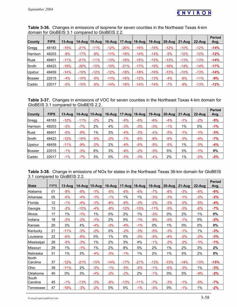
September 2004
H:\etcog3\report\sept04\sec3.doc 3-58
Table 3-36. Changes in emissions of isoprene for seven counties in the Northeast Texas 4-km domain for GloBEIS 3.1 compared to GloBEIS 2.2.
County FIPS 13-Aug 14-Aug 15-Aug 16-Aug 17-Aug 18-Aug 19-Aug 20-Aug 21-Aug 22-AugPeriod Avg.
Gregg 48183 -15% -21% -11% -12% -20% -16% -16% -12% -10% -12% -14%
Harrison 48203 -8% -17% -9% -11% -16% -14% -14% -9% -10% -10% -12%
Rusk 48401 -11% -21% -11% -13% -19% -15% -15% -13% -13% -13% -14%
Smith 48423 -15% -26% -15% -15% -21% -17% -16% -16% -14% -14% -17%
Upshur 48459 -14% -19% -12% -12% -18% -18% -16% -13% -10% -13% -14%
Bossier 22015 -4% -10% -5% -11% -16% -12% -13% -4% -6% -11% -9%
Caddo 22017 -5% -15% -8% -14% -18% -14% -14% -7% -9% -13% -12% Table 3-37. Changes in emissions of VOC for seven counties in the Northeast Texas 4-km domain for GloBEIS 3.1 compared to GloBEIS 2.2.
County FIPS 13-Aug 14-Aug 15-Aug 16-Aug 17-Aug 18-Aug 19-Aug 20-Aug 21-Aug 22-AugPeriod Avg.
Gregg 48183 -12% -11% -2% 2% -6% -6% -6% -4% -1% -2% -5%
Harrison 48203 -5% -7% 2% 4% -3% -3% -3% -1% 1% 0% -1%
Rusk 48401 -6% -9% 1% 3% -4% -3% -4% -5% -1% -1% -3%
Smith 48423 -12% -16% -5% -2% -7% -6% -6% -9% -3% -4% -7%
Upshur 48459 -11% -9% -2% 2% -4% -6% -5% -5% 1% -3% -4%
Bossier 22015 -1% -3% 6% 3% -4% -2% -3% 5% 3% -1% 0%
Caddo 22017 -1% -7% 3% 0% -5% -3% -4% 2% 1% -2% -2% Table 3-38. Change in emissions of NOx for states in the Northeast Texas 36-km domain for GloBEIS 3.1 compared to GloBEIS 2.2.
State FIPS 13-Aug 14-Aug 15-Aug 16-Aug 17-Aug 18-Aug 19-Aug 20-Aug 21-Aug 22-AugPeriod Avg.
Alabama 01 -8% -8% -1% -5% -6% -6% -7% -8% -3% -6% -6% Arkansas 05 -6% -4% -1% -1% 1% 1% -3% -3% -1% -2% -2% Florida 12 -1% -4% -1% -6% -8% -3% -2% -3% -3% -5% -4% Georgia 13 -2% -10% -4% -8% -12% -13% -11% -5% -3% -6% -7% Illinois 17 1% -1% 1% 0% 2% 1% -3% 0% 2% 1% 0% Indiana 18 -2% -2% -1% 2% 0% -1% -8% -5% -1% 0% -2% Kansas 20 3% 4% -4% -3% -4% -1% 0% 1% 0% 0% 0% Kentucky 21 -11% -3% -2% 0% -2% -3% -5% -3% -1% 1% -3% Louisiana 22 -6% -8% 0% 1% 0% -3% -5% -4% -2% -2% -3% Mississippi 28 -6% -3% 1% 2% 3% 4% -1% -2% -2% -1% -1% Missouri 29 1% -1% 1% 2% 8% 5% 2% 1% 2% 3% 2% Nebraska 31 1% 3% -4% -3% -1% 1% 2% 1% 0% 2% 0% North Carolina 37 -12% -21% -15% -14% -17% -21% -13% -13% -14% -13% -15% Ohio 39 -11% 2% -3% -1% -5% -6% -1% -6% -3% 1% -3% Oklahoma 40 0% 3% -4% -3% -2% 2% -1% 0% 0% -9% -2% South Carolina 45 -1% -13% -3% -9% -13% -11% -7% -3% -1% -5% -7% Tennessee 47 -10% -3% -2% 0% 0% -1% -3% 0% -1% 1% -2%

September 2004
H:\etcog3\report\sept04\sec3.doc 3-59
State FIPS 13-Aug 14-Aug 15-Aug 16-Aug 17-Aug 18-Aug 19-Aug 20-Aug 21-Aug 22-AugPeriod Avg.
Virginia 51 -8% -6% -6% 0% -1% -5% -3% -6% -6% 2% -4% West Virginia 54 5% 9% 2% 3% 0% -3% 7% 3% -1% 7% 3% Table 3-39. Change in emissions of CO for states in the Northeast Texas 36-km domain for GloBEIS 3.1 compared to GloBEIS 2.2.
State FIPS 13-Aug 14-Aug 15-Aug 16-Aug 17-Aug 18-Aug 19-Aug 20-Aug 21-Aug 22-AugPeriod Avg.
Alabama 01 -15% -15% -3% -10% -14% -13% -18% -17% -8% -15% -13% Arkansas 05 -17% -13% -9% -8% -9% -9% -18% -12% -9% -13% -12% Florida 12 -5% -8% -3% -10% -13% -6% -5% -6% -5% -9% -7% Georgia 13 -27% -37% -31% -36% -39% -39% -38% -33% -30% -32% -34% Illinois 17 -1% -3% 2% -3% -3% -5% -4% -1% -1% -4% -2% Indiana 18 -18% -16% -18% -15% -19% -22% -27% -22% -20% -18% -19% Kansas 20 3% 3% -10% -11% -7% -7% -5% -3% -6% -6% -5% Kentucky 21 -47% -40% -46% -45% -48% -48% -46% -46% -46% -39% -45% Louisiana 22 -17% -17% -10% -10% -14% -18% -20% -16% -15% -18% -16% Mississippi 28 -12% -10% -8% -8% -10% -8% -13% -17% -16% -14% -12% Missouri 29 1% -3% 0% -2% 5% 3% -1% -2% -1% -4% 0% Nebraska 31 2% 4% -6% -4% 0% 2% 1% 1% -3% 1% 0% North Carolina 37 -27% -36% -34% -35% -38% -42% -36% -32% -34% -30% -34% Ohio 39 -78% -75% -79% -79% -80% -80% -79% -80% -79% -22% -73% Oklahoma 40 -15% -11% -16% -13% -12% -9% -12% -11% -9% -17% -12% South Carolina 45 -33% -43% -37% -43% -46% -44% -42% -37% -35% -27% -39% Tennessee 47 -21% -13% -15% -12% -15% -17% -20% -15% -15% -16% -16% Virginia 51 -54% -51% -55% -51% -51% -54% -53% -54% -54% -43% -52% West Virginia 54 -56% -55% -65% -65% -66% -67% -62% -65% -66% -19% -59% Table 3-40. Change in emissions of isoprene for states in the Northeast Texas 36-km domain for GloBEIS 3.1 compared to GloBEIS 2.2.
State FIPS 13-Aug 14-Aug 15-Aug 16-Aug 17-Aug 18-Aug 19-Aug 20-Aug 21-Aug 22-AugPeriod Avg.
Alabama 01 -19% -20% -5% -14% -16% -15% -21% -21% -12% -21% -16% Arkansas 05 -13% -11% -10% -13% -16% -14% -17% -12% -11% -18% -14% Florida 12 -13% -22% -3% -9% -17% -6% -4% -8% -5% -11% -10% Georgia 13 -30% -39% -26% -33% -39% -36% -36% -33% -26% -29% -33% Illinois 17 0% -6% 0% -6% -6% -8% -7% -2% -6% -11% -5% Indiana 18 -16% -13% -14% -12% -20% -22% -19% -19% -18% -17% -17% Kansas 20 6% 1% -12% -9% -9% -11% -8% -8% -11% -13% -8% Kentucky 21 -45% -33% -43% -41% -46% -46% -42% -39% -44% -38% -42% Louisiana 22 -13% -20% -14% -17% -19% -21% -22% -17% -17% -23% -18% Mississippi 28 -10% -11% -7% -14% -15% -13% -15% -16% -17% -19% -14% Missouri 29 5% -5% 1% -3% 5% 3% -4% -2% -4% -10% -1% Nebraska 31 -1% -1% -9% -9% -1% 2% -3% 0% -8% -1% -3%

September 2004
H:\etcog3\report\sept04\sec3.doc 3-60
State FIPS 13-Aug 14-Aug 15-Aug 16-Aug 17-Aug 18-Aug 19-Aug 20-Aug 21-Aug 22-AugPeriod Avg.
North Carolina 37 -34% -43% -36% -38% -43% -48% -38% -39% -38% -38% -39% Ohio 39 -78% -72% -80% -80% -81% -80% -79% -79% -80% -18% -73% Oklahoma 40 -14% -10% -16% -14% -16% -14% -14% -15% -10% -16% -14% South Carolina 45 -40% -44% -32% -41% -47% -44% -40% -37% -33% -28% -39% Tennessee 47 -18% -13% -15% -12% -19% -19% -21% -13% -17% -22% -17% Virginia 51 -54% -54% -60% -52% -52% -53% -56% -56% -56% -43% -54% West Virginia 54 -53% -46% -65% -63% -65% -64% -61% -59% -64% -16% -55% Table 3-41. Change in emissions of VOC for states in the Northeast Texas 36-km domain for GloBEIS 3.1 compared to GloBEIS 2.2.
State FIPS 13-Aug 14-Aug 15-Aug 16-Aug 17-Aug 18-Aug 19-Aug 20-Aug 21-Aug 22-AugPeriod Avg.
Alabama 01 -10% -10% 5% -4% -7% -6% -13% -11% -2% -10% -7% Arkansas 05 -6% -3% -1% -3% -6% -4% -10% -3% -1% -8% -5% Florida 12 3% -2% 10% 2% -4% 6% 7% 5% 7% 2% 4% Georgia 13 -17% -29% -16% -23% -29% -27% -27% -21% -15% -20% -22% Illinois 17 9% 5% 10% 3% 3% 4% 4% 8% 4% -1% 5% Indiana 18 -7% 1% -4% -2% -10% -11% -10% -9% -7% -7% -7% Kansas 20 19% 15% -1% 1% 3% 2% 5% 8% 3% 4% 6% Kentucky 21 -37% -20% -32% -32% -37% -37% -33% -29% -34% -28% -32% Louisiana 22 -5% -9% -1% -3% -6% -10% -11% -6% -5% -10% -7% Mississippi 28 -2% -2% 2% -3% -4% -2% -6% -8% -8% -9% -4% Missouri 29 12% 3% 8% 4% 12% 11% 4% 6% 4% -2% 6% Nebraska 31 15% 12% 2% 3% 11% 14% 11% 13% 5% 14% 10% North Carolina 37 -25% -36% -28% -30% -35% -41% -30% -29% -29% -29% -31% Ohio 39 -67% -49% -66% -68% -70% -69% -64% -66% -68% -6% -59% Oklahoma 40 -7% -2% -9% -6% -8% -6% -6% -6% -2% -9% -6% South Carolina 45 -26% -35% -22% -31% -37% -34% -31% -25% -22% -18% -28% Tennessee 47 -12% -3% -6% -4% -10% -11% -13% -3% -8% -12% -8% Virginia 51 -45% -43% -47% -42% -43% -44% -46% -44% -45% -33% -43% West Virginia 54 -43% -29% -52% -53% -56% -55% -50% -46% -54% -5% -44%
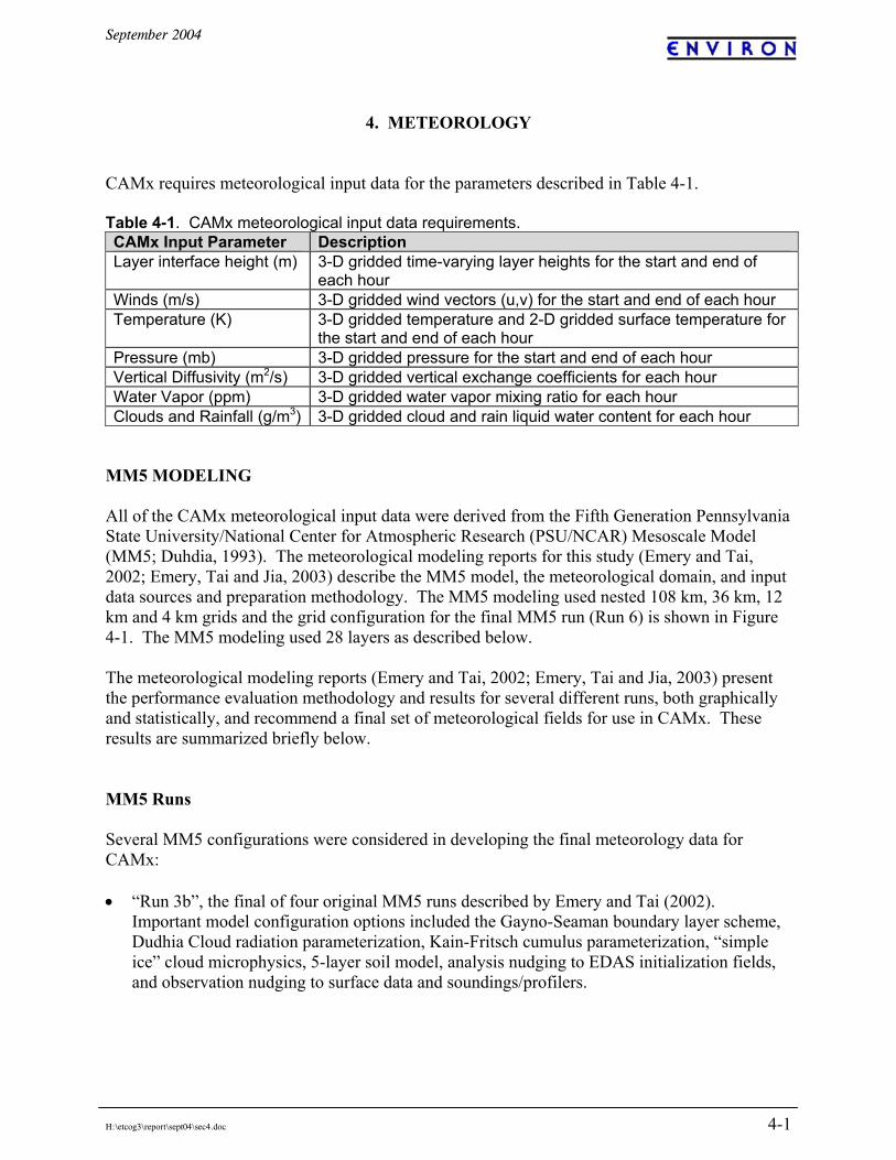
September 2004
H:\etcog3\report\sept04\sec4.doc 4-1
4. METEOROLOGY CAMx requires meteorological input data for the parameters described in Table 4-1. Table 4-1. CAMx meteorological input data requirements. CAMx Input Parameter Description Layer interface height (m) 3-D gridded time-varying layer heights for the start and end of
each hour Winds (m/s) 3-D gridded wind vectors (u,v) for the start and end of each hour Temperature (K) 3-D gridded temperature and 2-D gridded surface temperature for
the start and end of each hour Pressure (mb) 3-D gridded pressure for the start and end of each hour Vertical Diffusivity (m2/s) 3-D gridded vertical exchange coefficients for each hour Water Vapor (ppm) 3-D gridded water vapor mixing ratio for each hour Clouds and Rainfall (g/m3) 3-D gridded cloud and rain liquid water content for each hour
MM5 MODELING All of the CAMx meteorological input data were derived from the Fifth Generation Pennsylvania State University/National Center for Atmospheric Research (PSU/NCAR) Mesoscale Model (MM5; Duhdia, 1993). The meteorological modeling reports for this study (Emery and Tai, 2002; Emery, Tai and Jia, 2003) describe the MM5 model, the meteorological domain, and input data sources and preparation methodology. The MM5 modeling used nested 108 km, 36 km, 12 km and 4 km grids and the grid configuration for the final MM5 run (Run 6) is shown in Figure 4-1. The MM5 modeling used 28 layers as described below. The meteorological modeling reports (Emery and Tai, 2002; Emery, Tai and Jia, 2003) present the performance evaluation methodology and results for several different runs, both graphically and statistically, and recommend a final set of meteorological fields for use in CAMx. These results are summarized briefly below. MM5 Runs Several MM5 configurations were considered in developing the final meteorology data for CAMx: • “Run 3b”, the final of four original MM5 runs described by Emery and Tai (2002).
Important model configuration options included the Gayno-Seaman boundary layer scheme, Dudhia Cloud radiation parameterization, Kain-Fritsch cumulus parameterization, “simple ice” cloud microphysics, 5-layer soil model, analysis nudging to EDAS initialization fields, and observation nudging to surface data and soundings/profilers.
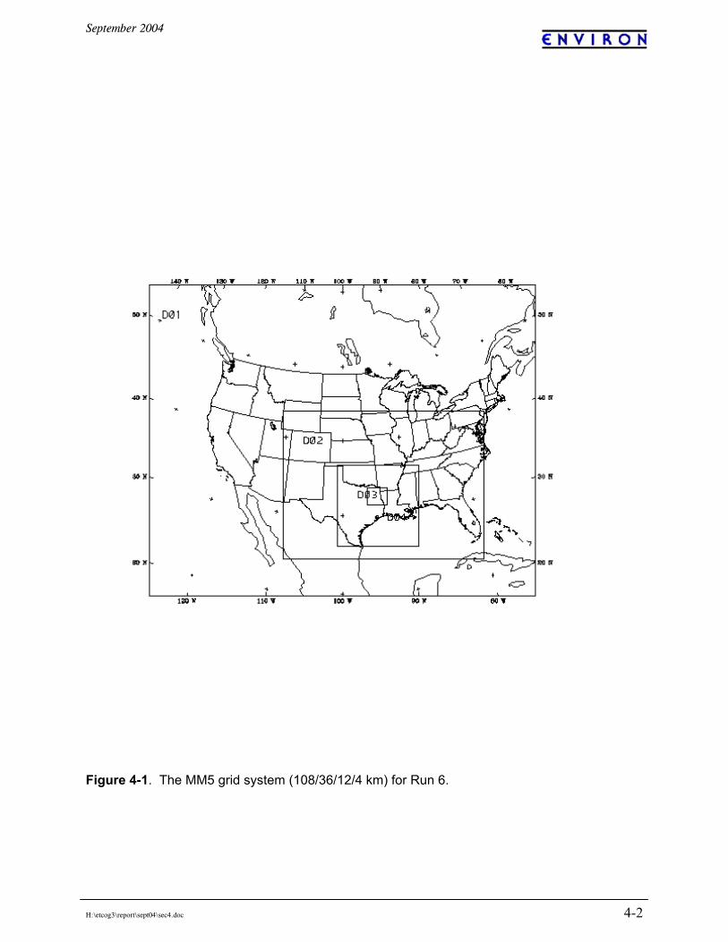
September 2004
H:\etcog3\report\sept04\sec4.doc 4-2
Figure 4-1. The MM5 grid system (108/36/12/4 km) for Run 6.
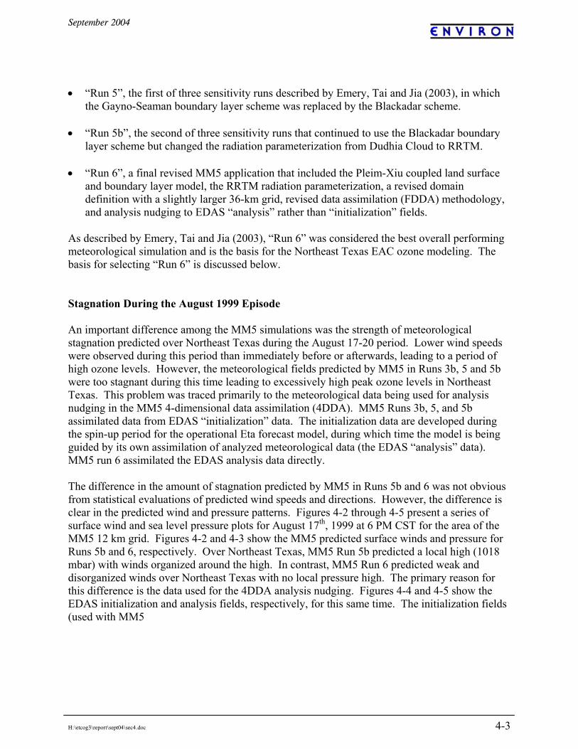
September 2004
H:\etcog3\report\sept04\sec4.doc 4-3
• “Run 5”, the first of three sensitivity runs described by Emery, Tai and Jia (2003), in which
the Gayno-Seaman boundary layer scheme was replaced by the Blackadar scheme. • “Run 5b”, the second of three sensitivity runs that continued to use the Blackadar boundary
layer scheme but changed the radiation parameterization from Dudhia Cloud to RRTM. • “Run 6”, a final revised MM5 application that included the Pleim-Xiu coupled land surface
and boundary layer model, the RRTM radiation parameterization, a revised domain definition with a slightly larger 36-km grid, revised data assimilation (FDDA) methodology, and analysis nudging to EDAS “analysis” rather than “initialization” fields.
As described by Emery, Tai and Jia (2003), “Run 6” was considered the best overall performing meteorological simulation and is the basis for the Northeast Texas EAC ozone modeling. The basis for selecting “Run 6” is discussed below. Stagnation During the August 1999 Episode An important difference among the MM5 simulations was the strength of meteorological stagnation predicted over Northeast Texas during the August 17-20 period. Lower wind speeds were observed during this period than immediately before or afterwards, leading to a period of high ozone levels. However, the meteorological fields predicted by MM5 in Runs 3b, 5 and 5b were too stagnant during this time leading to excessively high peak ozone levels in Northeast Texas. This problem was traced primarily to the meteorological data being used for analysis nudging in the MM5 4-dimensional data assimilation (4DDA). MM5 Runs 3b, 5, and 5b assimilated data from EDAS “initialization” data. The initialization data are developed during the spin-up period for the operational Eta forecast model, during which time the model is being guided by its own assimilation of analyzed meteorological data (the EDAS “analysis” data). MM5 run 6 assimilated the EDAS analysis data directly. The difference in the amount of stagnation predicted by MM5 in Runs 5b and 6 was not obvious from statistical evaluations of predicted wind speeds and directions. However, the difference is clear in the predicted wind and pressure patterns. Figures 4-2 through 4-5 present a series of surface wind and sea level pressure plots for August 17th, 1999 at 6 PM CST for the area of the MM5 12 km grid. Figures 4-2 and 4-3 show the MM5 predicted surface winds and pressure for Runs 5b and 6, respectively. Over Northeast Texas, MM5 Run 5b predicted a local high (1018 mbar) with winds organized around the high. In contrast, MM5 Run 6 predicted weak and disorganized winds over Northeast Texas with no local pressure high. The primary reason for this difference is the data used for the 4DDA analysis nudging. Figures 4-4 and 4-5 show the EDAS initialization and analysis fields, respectively, for this same time. The initialization fields (used with MM5
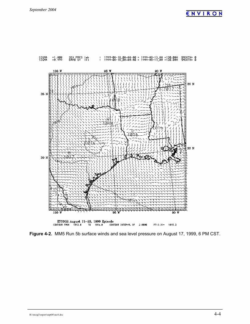
September 2004
H:\etcog3\report\sept04\sec4.doc 4-4
Figure 4-2. MM5 Run 5b surface winds and sea level pressure on August 17, 1999, 6 PM CST.

September 2004
H:\etcog3\report\sept04\sec4.doc 4-5
Figure 4-3. MM5 Run 6 surface winds and sea level pressure on August 17, 1999, 6 PM CST.
September 2004
H:\etcog3\report\sept04\sec4.doc 4-6
Figure 4-4. EDAS “initialization” surface winds and sea level pressure used to nudge MM5 Run 5B on August 17, 1999, 6 PM CST.
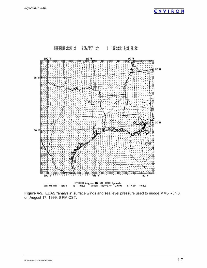
September 2004
H:\etcog3\report\sept04\sec4.doc 4-7
Figure 4-5. EDAS “analysis” surface winds and sea level pressure used to nudge MM5 Run 6 on August 17, 1999, 6 PM CST.

September 2004
H:\etcog3\report\sept04\sec4.doc 4-8
Run 5b) have higher pressure over Northeast Texas than the analysis fields (used with MM5 Run 6). Comparison of the EDAS fields to archived daily weather maps showed that high pressure in Northeast Texas was over-stated by the EDAS initialization fields. The modeled and observed winds and temperatures at Longview (CAMS 19) are compared in Figures 4-6 and 4-7, respectively. Overall, both runs replicate the observed winds quite well and it is difficult to say that one or other is better. Both follow the observed speed trends well, but both generally over predicted by about 1 m/s on average. The same general conclusions are reached for wind direction, although Run 5b perhaps indicates a slightly more noisy performance. The temperature predictions show that Run 6 was generally too warm during the day during the mid to late portions of the episode. Run 5b generally under predicted temperatures during much of the period. Overall, Run 6 provides a better balance for temperature performance. Boundary Layer Depths Vertical profiles of observed wind, temperature and humidity from Shreveport and Palestine were compared to the soundings simulated by MM5 in Runs 3b, 5b, and 6. In Shreveport, Runs 5b and 6 typically performed better for winds than Run 3b (with Run 6 the best overall), which we believe is related to the issues identified with the Gayno-Seaman boundary layer scheme used in Run 3b. While Run 6 consistently over predicted the temperature profile in the boundary layer, it agreed most closely with the observed profile. Runs 3b and 5b were cooler than observed through the boundary layer, and generally indicated more static stability and slightly lower mixing depths than observed. Run 6 also typically performed better for boundary layer humidity than the other runs (least error), but humidity was often slightly under predicted. Usually, Runs 3b and 5b over estimated surface and boundary layer humidity. While Runs 3b and 5b seemed to place the top of the boundary layer near or below the observed level, the mixing depth in Run 6 was higher than observed. Very similar results were seen for the three MM5 simulations at the Palestine site. The spatial patterns of boundary layer heights over the south-central U.S. were further assessed for Runs 5b and 6. Run 6, which used the Plein-Xiu coupled surface-boundary layer model, consistently developed deeper mixing depths throughout the south-central U.S. than Run 5b, which used the Blackadar boundary layer model. Typically, the Run 5b depths over East Texas ranged from 1000 – 2000 m, whereas the Run 6 depths were usually 2000-2500 m. Run 3b generated mixing depths similar to Run 5b but the mixing depths showed large spatial variability that was unreasonable and appeared to be an artifact of the Gayno-Seaman boundary layer scheme. This characteristic may have the largest impacts on air quality simulations, far more than any wind or temperature differences.
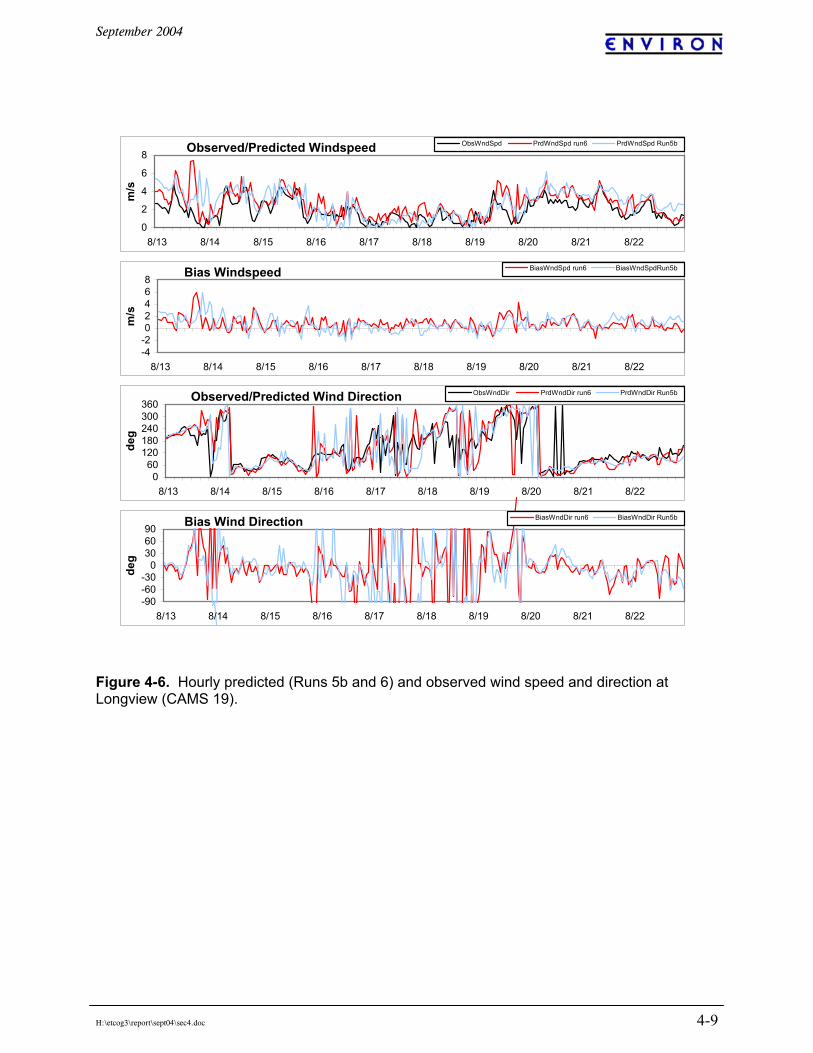
September 2004
H:\etcog3\report\sept04\sec4.doc 4-9
Figure 4-6. Hourly predicted (Runs 5b and 6) and observed wind speed and direction at Longview (CAMS 19).
Observed/Predicted Windspeed
0
2
4
6
8
8/13 8/14 8/15 8/16 8/17 8/18 8/19 8/20 8/21 8/22
m/s
ObsWndSpd PrdWndSpd run6 PrdWndSpd Run5b
Bias Windspeed
-4-202468
8/13 8/14 8/15 8/16 8/17 8/18 8/19 8/20 8/21 8/22
m/s
BiasWndSpd run6 BiasWndSpdRun5b
Observed/Predicted Wind Direction
060
120180240300360
8/13 8/14 8/15 8/16 8/17 8/18 8/19 8/20 8/21 8/22
deg
ObsWndDir PrdWndDir run6 PrdWndDir Run5b
Bias Wind Direction
-90-60-30
0306090
8/13 8/14 8/15 8/16 8/17 8/18 8/19 8/20 8/21 8/22
deg
BiasWndDir run6 BiasWndDir Run5b

September 2004
H:\etcog3\report\sept04\sec4.doc 4-10
Figure 4-7. Hourly predicted (Runs 5b and 6) and observed temperature at Longview (CAMS 19).
Observed/Predicted Temperature
280
285
290
295
300
305
310
315
8/13 8/14 8/15 8/16 8/17 8/18 8/19 8/20 8/21 8/22
KObsTemp PrdTemp run6 PrdTemp Run5b
Bias Temperature
-12-10-8-6-4-20246
8/13 8/14 8/15 8/16 8/17 8/18 8/19 8/20 8/21 8/22
K
BiasTemp run 6 BiasTemp Run5b

September 2004
H:\etcog3\report\sept04\sec4.doc 4-11
CAMx INPUT DATA PREPARATION MM5 output fields were translated to CAMx-ready inputs using ENVIRON’s MM5CAMx translation software. This program performs several functions: 1. Extracts wind, temperature, pressure, humidity, cloud, and rain fields from each MM5 grid
that matches the corresponding CAMx grid. 2. Performs mass-weighted vertical aggregation of data for CAMx layers that span multiple
MM5 layers. 3. Diagnoses fields of vertical diffusion coefficient (Kv), which are not directly output by
MM5. 4. Outputs the meteorological data into CAMx-ready input files. The MM5CAMx program has been written to carefully preserve the consistency of the predicted wind, temperature and pressure fields output by MM5. This is the key to preparing mass-consistent inputs, and therefore for obtaining the best possible performance from CAMx. The data prepared by MM5CAMx were directly input to CAMx. Meteorological inputs were developed for a 15-layer CAMx application (Figure 4-8). Every MM5 layer below ~3800m above ground level was mapped directly to a CAMx layer. The CAMx surface layer was ~20 m deep. Vertical diffusivities are an important input to the CAMx simulation since they determine the rate and depth of mixing in the planetary boundary layer (PBL) and above. In general, diffusivities directly output from meteorological models, or diffusivities diagnosed from other output variables, require careful examination before they are used in air quality modeling. This may be because the air quality model results are much more sensitive to diffusivities than the meteorological model results. In CAMx simulations using meteorology from MM5 “Run 3b” the vertical diffusivities were calculated from output fields of turbulent kinetic energy predicted by the Gayno-Seaman boundary layer model. This approach is preferred as it provides a direct means to translate turbulence intensity in MM5 to diffusion rates in CAMx. For MM5 simulations “Run 5,” “Run 5b”and “Run 6” the MM5 boundary layer (mixing) depths were used to define a profile of vertical diffusivity values in each grid column, depending on surface layer stability and the underlying surface characteristics. The methodology follows from O’Brien (1970). This method was necessary because the Blackadar and Pleim-Xiu PBL schemes do not generate fields of turbulent kinetic energy.

September 2004
H:\etcog3\report\sept04\sec4.doc 4-12
Layer sigma pressure height thickness CAMx Layers ===========================================| |================== 28 0.0000 50.00 18874.41 1706.76 27 0.0250 73.75 17167.65 1362.47 26 0.0500 97.50 15805.17 2133.42 25 0.1000 145.00 13671.75 1664.35 24 0.1500 192.50 12007.40 1376.75 23 0.2000 240.00 10630.65 1180.35 22 0.2500 287.50 9450.30 1036.79 21 0.3000 335.00 8413.52 926.80 20 0.3500 382.50 7486.72 839.57 19 0.4000 430.00 6647.15 768.53 18 0.4500 477.50 5878.62 709.45 17 0.5000 525.00 5169.17 659.47 16 0.5500 572.50 4509.70 616.58 15 0.6000 620.00 3893.12 579.34 --15--- 14 0.6500 667.50 3313.78 546.67 --14--- 13 0.7000 715.00 2767.11 517.77 --13--- 12 0.7500 762.50 2249.35 491.99 --12--- 11 0.8000 810.00 1757.36 376.81 --11--- 10 0.8400 848.00 1380.55 273.60 --10--- 9 0.8700 876.50 1106.95 266.37 ---9--- 8 0.9000 905.00 840.58 259.54 ---8--- 7 0.9300 933.50 581.04 169.41 ---7--- 6 0.9500 952.50 411.63 166.65 ---6--- 5 0.9700 971.50 244.98 82.31 ---5--- 4 0.9800 981.00 162.67 65.38 ---4--- 3 0.9880 988.60 97.29 56.87 ---3--- 2 0.9950 995.25 40.43 20.23 ---2--- 1 0.9975 997.62 20.19 20.19 ---1--- 0 1.0000 1000.00 0.00 =============Surface====== Figure 4-8. MM5 and CAMx vertical grid structures based on 28 sigma-p levels. Heights (m) are above ground level according to a standard atmosphere; pressure is in millibars.
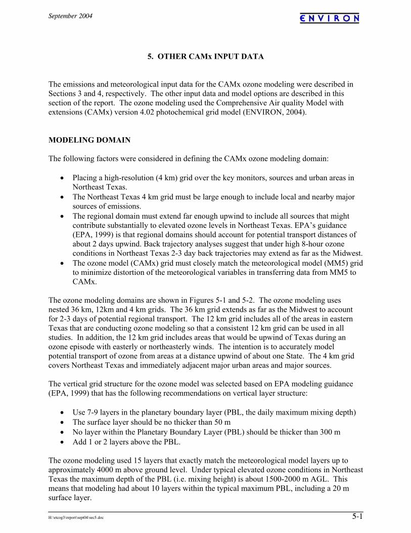
September 2004
H:\etcog3\report\sept04\sec5.doc 5-1
5. OTHER CAMx INPUT DATA The emissions and meteorological input data for the CAMx ozone modeling were described in Sections 3 and 4, respectively. The other input data and model options are described in this section of the report. The ozone modeling used the Comprehensive Air quality Model with extensions (CAMx) version 4.02 photochemical grid model (ENVIRON, 2004). MODELING DOMAIN The following factors were considered in defining the CAMx ozone modeling domain:
• Placing a high-resolution (4 km) grid over the key monitors, sources and urban areas in Northeast Texas.
• The Northeast Texas 4 km grid must be large enough to include local and nearby major sources of emissions.
• The regional domain must extend far enough upwind to include all sources that might contribute substantially to elevated ozone levels in Northeast Texas. EPA’s guidance (EPA, 1999) is that regional domains should account for potential transport distances of about 2 days upwind. Back trajectory analyses suggest that under high 8-hour ozone conditions in Northeast Texas 2-3 day back trajectories may extend as far as the Midwest.
• The ozone model (CAMx) grid must closely match the meteorological model (MM5) grid to minimize distortion of the meteorological variables in transferring data from MM5 to CAMx.
The ozone modeling domains are shown in Figures 5-1 and 5-2. The ozone modeling uses nested 36 km, 12km and 4 km grids. The 36 km grid extends as far as the Midwest to account for 2-3 days of potential regional transport. The 12 km grid includes all of the areas in eastern Texas that are conducting ozone modeling so that a consistent 12 km grid can be used in all studies. In addition, the 12 km grid includes areas that would be upwind of Texas during an ozone episode with easterly or northeasterly winds. The intention is to accurately model potential transport of ozone from areas at a distance upwind of about one State. The 4 km grid covers Northeast Texas and immediately adjacent major urban areas and major sources. The vertical grid structure for the ozone model was selected based on EPA modeling guidance (EPA, 1999) that has the following recommendations on vertical layer structure:
• Use 7-9 layers in the planetary boundary layer (PBL, the daily maximum mixing depth) • The surface layer should be no thicker than 50 m • No layer within the Planetary Boundary Layer (PBL) should be thicker than 300 m • Add 1 or 2 layers above the PBL.
The ozone modeling used 15 layers that exactly match the meteorological model layers up to approximately 4000 m above ground level. Under typical elevated ozone conditions in Northeast Texas the maximum depth of the PBL (i.e. mixing height) is about 1500-2000 m AGL. This means that modeling had about 10 layers within the typical maximum PBL, including a 20 m surface layer.

September 2004
H:\etcog3\report\sept04\sec5.doc 5-2
Figure 5-1. CAMx modeling domain for the August 1999 episode showing the 36 km regional grid and the nested 12 km and 4 km fine grids.
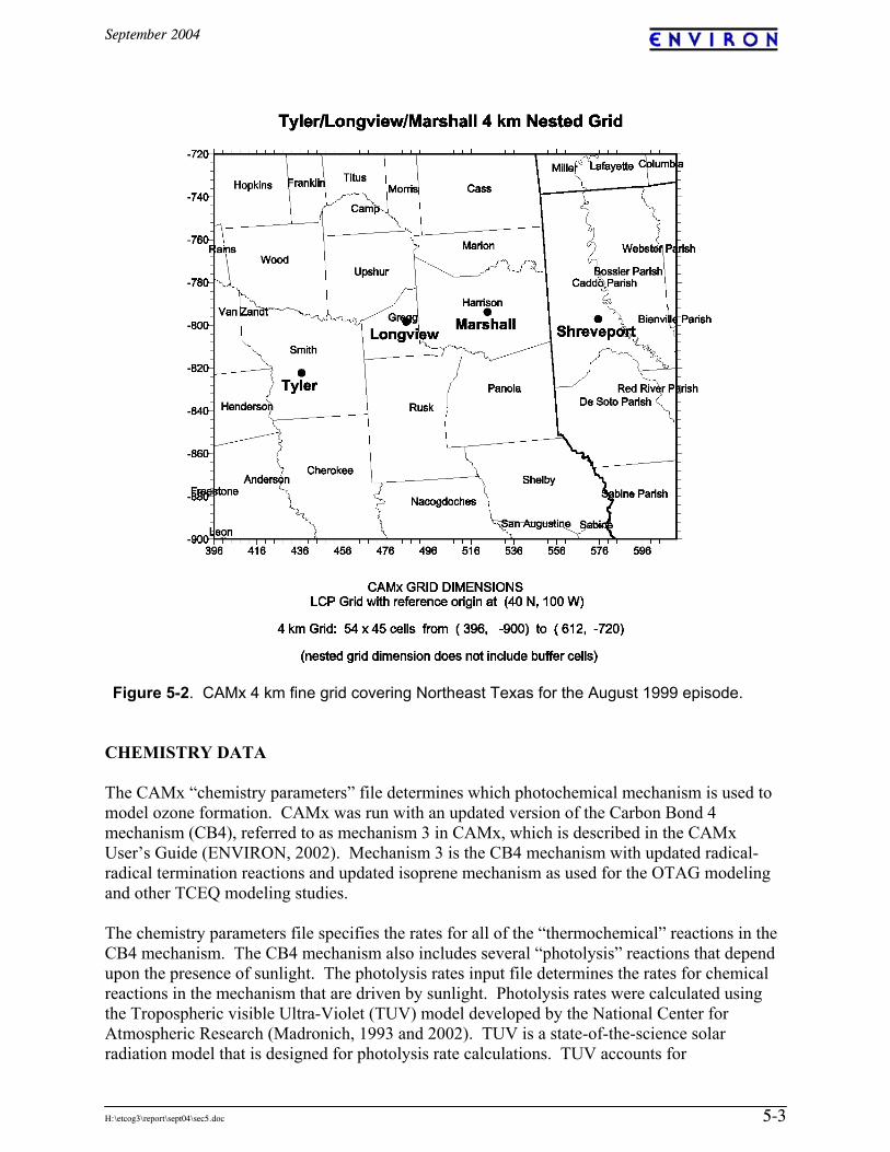
September 2004
H:\etcog3\report\sept04\sec5.doc 5-3
Figure 5-2. CAMx 4 km fine grid covering Northeast Texas for the August 1999 episode.
CHEMISTRY DATA The CAMx “chemistry parameters” file determines which photochemical mechanism is used to model ozone formation. CAMx was run with an updated version of the Carbon Bond 4 mechanism (CB4), referred to as mechanism 3 in CAMx, which is described in the CAMx User’s Guide (ENVIRON, 2002). Mechanism 3 is the CB4 mechanism with updated radical-radical termination reactions and updated isoprene mechanism as used for the OTAG modeling and other TCEQ modeling studies. The chemistry parameters file specifies the rates for all of the “thermochemical” reactions in the CB4 mechanism. The CB4 mechanism also includes several “photolysis” reactions that depend upon the presence of sunlight. The photolysis rates input file determines the rates for chemical reactions in the mechanism that are driven by sunlight. Photolysis rates were calculated using the Tropospheric visible Ultra-Violet (TUV) model developed by the National Center for Atmospheric Research (Madronich, 1993 and 2002). TUV is a state-of-the-science solar radiation model that is designed for photolysis rate calculations. TUV accounts for

September 2004
H:\etcog3\report\sept04\sec5.doc 5-4
environmental parameters that influence photolysis rates including solar zenith angle, altitude above the ground, surface UV albedo, aerosols (haze), and stratospheric ozone column. The albedo/haze/ozone input file is used in conjunction with the photolysis rates input file to specify several of the environmental factors that influence photoloysis rates. The photolysis rates and albedo/haze/ozone files must be coordinated to function together correctly. The surface UV albedo was calculated based on the gridded land use data using the landuse specific UV albedo values given in Table 5-1. The albedo varies spatially according to the land cover distribution, but does not vary with time. The total ozone column was based on satellite data from the Total Ozone Mapping Spectrometer (TOMS), which are available from a web site maintained by the NASA Goddard Space Flight Center (http://jwocky.gsfc.nasa.gov). Daily ozone column are available at 1.25°longitude by 1° latitude resolution and were mapped to the CAMx grid. The haze optical depth was assumed to be 0.1. Table 5-1. CAMx land use categories and the default surface roughness values (m) and UV albedo assigned to each category within CAMx.
Category Number
Land Cover Category
Surface Roughness
(meters)
UV
Albedo 1 Urban 3.00 0.08 2 Agricultural 0.25 0.05 3 Rangeland 0.05 0.05 4 Deciduous forest 1.00 0.05 5 Coniferous forest including wetland 1.00 0.05 6 Mixed forest 1.00 0.05 7 Water 0.0001 0.04 8 Barren land 0.002 0.08 9 Non-forested wetlands 0.15 0.05
10 Mixed agricultural and range 0.10 0.05 11 Rocky (with low shrubs) 0.10 0.05
INITIAL AND BOUNDARY CONDITIONS The initial conditions (ICs) are the pollutant concentrations specified throughout the modeling domain at the start of the simulation. Boundary conditions (BCs) are the pollutant concentrations specified at the perimeter of the modeling domain throughout the simulation. The boundary condition assumptions are discussed because they played a role in achieving good ozone model performance. The boundary conditions are shown in Table 5-2. The ozone BC was set to 40 ppb, which is the value commonly considered to be the continental background and used for ozone modeling studies. The NOx BC was set to 1.1 ppb. The VOC BCs varied by boundary segment over a range from 9 to 50 ppbC according to broad differences in land cover. The higher VOC BCs in the Northeast/East boundary segment are for areas with higher biogenic emissions (Goldan et al., 1995; Watkins et al., 1995). The lower VOC BCs along the West boundary segment are for dryer areas with lower biogenic emissions. The lowest VOC BCs are over the Gulf of Mexico and these low values were also used for all boundaries above an altitude of 1700 m. The initial conditions throughout the modeling domain were set to the lowest (Gulf of Mexico) BC values.

September 2004
H:\etcog3\report\sept04\sec5.doc 5-5
Figure 5-3. CAMx 36 km regional modeling domain showing boundary segments that are assigned different boundary conditions (BCs). Table 5-2. Boundary concentrations for different boundary segments shown in Figure 5-3. Species East/Northeastern
Boundary Western Boundary
Southern Boundary
O3 (ppb) 40.0 40.0 40.0 NOx (ppb) 1.1 1.1 1.1 VOC (ppbC) 50.5 22.3 9.3 SURFACE CHARACTERISTICS (LANDUSE) CAMx requires gridded landuse data to characterize surface boundary conditions, such as surface roughness, deposition parameters, vegetative distribution, and water/land boundaries. CAMx land use files provide the fractional contribution (0 to 1) of eleven land use categories (Table 5-2) to the surface area of grid cell. Gridded land cover data were developed from the same landuse databases that were used in the generation of spatial emission surrogates (Yarwood et al., 2002). A program was written to re-cast the raw spatial surrogate data into the eleven CAMx land use categories, to grid the data to the 36, 12, and 4 km CAMx grids, and to write the results to a model-ready format. Figures 5-4 and 5-5 show the dominant land use category in each grid cell for the 36 km and 12 km grids, respectively. The dominant land use comprises the majority of surface cover in each cell and the “Forest” category is the sum of the three CAMx categories 4 to 6.

September 2004
H:\etcog3\report\sept04\sec5.doc 5-6
Figure 5-4. Distribution of the dominant land cover type in each grid cell of the 36-km CAMx grid.
-108 252 612 972 1332LCP Easting (km)
-1584
-1224
-864
-504
-144
LCP
Nor
thin
g (k
m)
Distribution of Dominant Landuse36 km Extent at 36 km Resolution
Urba
n
Agric
ultu
reRa
ngel
and
Fore
st
Wat
er
Barre
n
Wet
land
sM
ixed
Ag/R
ange
Rock
y/lo
w sh
rubs
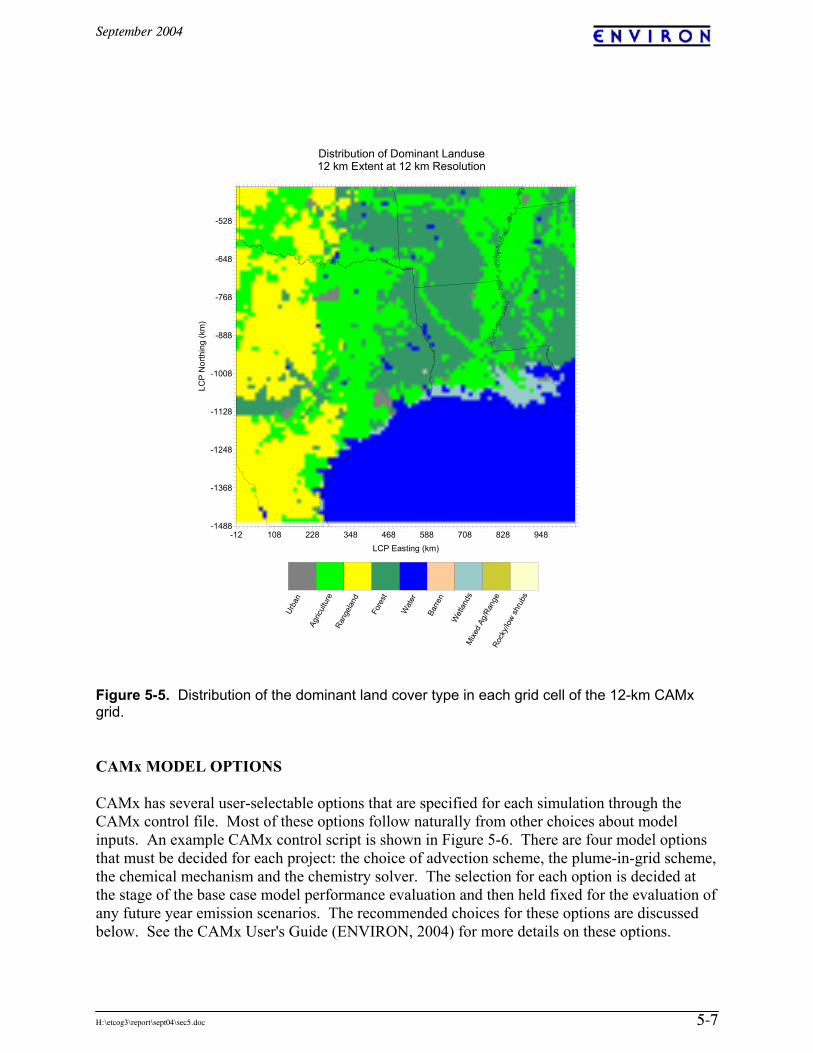
September 2004
H:\etcog3\report\sept04\sec5.doc 5-7
Figure 5-5. Distribution of the dominant land cover type in each grid cell of the 12-km CAMx grid. CAMx MODEL OPTIONS CAMx has several user-selectable options that are specified for each simulation through the CAMx control file. Most of these options follow naturally from other choices about model inputs. An example CAMx control script is shown in Figure 5-6. There are four model options that must be decided for each project: the choice of advection scheme, the plume-in-grid scheme, the chemical mechanism and the chemistry solver. The selection for each option is decided at the stage of the base case model performance evaluation and then held fixed for the evaluation of any future year emission scenarios. The recommended choices for these options are discussed below. See the CAMx User's Guide (ENVIRON, 2004) for more details on these options.
-12 108 228 348 468 588 708 828 948LCP Easting (km)
-1488
-1368
-1248
-1128
-1008
-888
-768
-648
-528
LCP
Nor
thin
g (k
m)
Distribution of Dominant Landuse12 km Extent at 12 km Resolution
Urba
n
Agric
ultu
reRa
ngel
and
Fore
st
Wat
er
Barre
n
Wet
land
sM
ixed
Ag/R
ange
Rock
y/lo
w sh
rubs

September 2004
H:\etcog3\report\sept04\sec5.doc 5-8
Advection Scheme CAMx version 4.02 has three optional methods for calculating horizontal advection (the movement of pollutants due to resolved horizontal winds) called Smolarkiewicz, Bott and Piecewise Parabolic Method (PPM). The Smolarkiewicz scheme has been used for many years, and was used in the previous modeling for Northeast Texas (ENVIRON, 1999). The Smolarkiewicz scheme has been criticized for causing too much artificial diffusion of pollutants, tending to "smear out" features and artificially overstate transport. The Bott and PPM schemes are newer and have less artificial diffusion than the Smolarkiewicz scheme. The PPM scheme was used for this study as it has been determined to be the least numerically diffusive, runs at speeds similar to Smolarkiewicz, and does not exhibit certain "noisy" features near sharp gradients that are apparent with the Bott approach. Plume-in-Grid CAMx includes an optional sub-grid scale plume model that can be used to represent the dispersion and chemistry of major NOx point source plumes close to the source. We used the Plume-in-Grid (PiG) sub-model for major NOx sources. Selection of PiG sources was discussed in Section 3. The criteria for selecting NOx point sources for plume in grid treatment within the 4-km modeling domain is 2 tons NOx on any episode day. For the regional emissions grid, the NOx criteria is 25 tons per day on any episode day. Chemical Mechanism CAMx provides several two main alternatives for the chemical mechanisms used to describe the gas-phase chemistry of ozone formation, namely the Carbon Bond 4 (CB4) and SAPRC99 mechanisms. The most widely used mechanism for regional applications is CB4 with the updated isoprene and radical termination reactions, and CB4 was used for this study. Chemistry Solver CAMx has two options for the numerical scheme used to solve the chemical mechanism. The first option is the CMC fast solver that has been used in every prior version of CAMx. The second option is an IEH solver. The CMC solver is faster and more accurate than most chemistry solvers used for ozone modeling. The IEH solver is even more accurate than the CMC solver, but slower. Both solvers were used during this study and the final base case 7 used the CMC solver.

September 2004
H:\etcog3\report\sept04\sec5.doc 5-9
CAMx Version |VERSION4.0 Run Message |CAMx v4.0 base7 Aug 13-22 1999 Root output name |../output/base7/camx.990816.base7 Start yr/mo/dy/hr |1999 08 16 0. End yr/mo/dy/hr |1999 08 16 2400. dtmx,dtin,dtem,dtou|15. 60. 60. 60. nx,ny,nz |45 46 15 Coordinate ID |LAMBERT xorg,yorg,dx,dy |-108. -1584. 36. 36. -100. 40. 60. 30. time zone |6 PiG parameters |2000. 12. Avg output species |16 |NO NO2 O3 PAR TOL ETH |OLE PAN ISOP XYL FORM ALD2 |HNO3 NXOY NTR CO # nested grids |2 nest grid params | 4 32 4 32 15 3 nest grid params |15 20 20 24 15 9 SMOLAR,BOTT, PPM? |PPM Chemistry solver |CMC Restart |true Chemistry |true Dry dep |true Wet dep |true PiG submodel |true Staggered winds |true Treat area emiss |true Treat point emiss |true 1-day emiss inputs |true 3-D average file |false Source Apportion |false Chemparam |../input/other/CAMx4.chemparam.3 Photolysis rates |../input/other/camx.etcog.rates.do Landuse |../input/other/CAMx.landuse.36km.lcp Height/pressure |../input/met/36km/camx.v4.zp.etcog.36km.990816.run6.bin.a0 Wind |../input/met/36km/camx.v4.uv.etcog.36km.990816.run6.bin.a0 Temperature |../input/met/36km/camx.v4.tp.etcog.36km.990816.run6.bin.a0 Water vapor |../input/met/36km/camx.v4.qa.etcog.36km.990816.run6.bin.a0 Cloud/Rain |../input/met/36km/camx.v4.cr.etcog.36km.990816.run6.bin.a0 Vertical diffsvty |../input/met/36km/camx.v4.kv.etcog.36km.990816.run6.patch.bin.a0 Initial conditions | Boundary conditions|../preproc/icbc_dfw/bc.36km.4km15.segments.bin Top concentration |../preproc/icbc_dfw/tc.36km.4km15.segments Albedo/haze/ozone |../input/other/ahomap.v4.etcog.aug99.drought.227-233 Point emiss |../eps2x/model_emiss/ptsrce.et3.pig.990816.a0 Area emiss |../eps2x/model_emiss/emiss.surface.ET3_reg_36km.drought.990816.a1 Landuse #1 |../input/other/CAMx.landuse.12km.lcp Landuse #2 |../input/other/CAMx.landuse.4km.buffered.lcp Height/pressure #1 |../input/met/12km/camx.v4.zp.etcog.12km.990816.run6.bin.a0 Height/pressure #2 |../input/met/04km/camx.v4.zp.etcog.04km.990816.run6.bin.a0 Wind #1 |../input/met/12km/camx.v4.uv.etcog.12km.990816.run6.bin.a0 Wind #2 |../input/met/04km/camx.v4.uv.etcog.04km.990816.run6.bin.a0 Temperature #1 |../input/met/12km/camx.v4.tp.etcog.12km.990816.run6.bin.a0 Temperature #2 |../input/met/04km/camx.v4.tp.etcog.04km.990816.run6.bin.a0 Water vapor #1 |../input/met/12km/camx.v4.qa.etcog.12km.990816.run6.bin.a0 Water vapor #2 |../input/met/04km/camx.v4.qa.etcog.04km.990816.run6.bin.a0 Cloud/Rain #1 |../input/met/12km/camx.v4.cr.etcog.12km.990816.run6.bin.a0 Cloud/Rain #2 |../input/met/04km/camx.v4.cr.etcog.04km.990816.run6.bin.a0 Vertical diff #1 |../input/met/12km/camx.v4.kv.etcog.12km.990816.run6.patch.bin.a0 Vertical diff #2 |../input/met/04km/camx.v4.kv.etcog.04km.990816.run6.patch.bin.a0 Area emiss #1 |../eps2x/model_emiss/emiss.surface.ET3_reg_12km_wbuf.drought.990816.a1 Area emiss #2 |../eps2x/model_emiss/emiss.surface.ET3_4km_wbuf.drought.990816.a0 coarse restart |../output/base7/camx.990815.base7.inst.2 fine restart |../output/base7/camx.990815.base7.finst.2 PiG restart |../output/base7/camx.990815.base7.pig Figure 5-6. Example CAMx control script for August 16th, 1999 of Base Case 7.

September 2004
H:\etcog3\report\sept04\sec6.doc 6-1
6. OZONE MODELING The ozone modeling for the Northeast Texas early action compact (EAC) followed the EPA’s draft guidance for 8-hour ozone modeling (EPA, 1999). The modeling procedures were established in a modeling protocol (ENVIRON, 2003). This section describes the modeling results, 8-hour ozone model performance evaluation and the 8-hour ozone attainment demonstration for 2007. OVERVIEW OF THE OZONE MODELING The ozone modeling began with developing a “base case” for the August 13-22, 1999 modeling period. Base case model performance was carefully evaluated to determine how well the modeling replicated observed ozone levels. The model performance evaluation compared the modeled and observed ozone levels and also considered whether the modeling was getting the right answer for the right reasons. Model sensitivity and diagnostic tests were an important tool for understanding the base case model performance and guiding efforts to correct specific problems that were hindering model performance. NETAC began developing an ozone model for the August 1999 episode before entering into the EAC, which allowed time for extensive model development and evaluation as described in a previous NETAC ozone modeling report (Yarwood et al., 2003). The ozone model development prior to the EAC led to a 1999 base case called “base5.” The development activities leading to base5 are summarized below including the results of numerous diagnostic and sensitivity tests. A new base case (base7) was developed for the EAC modeling using updated emission inventories, improved boundary conditions (BCs) and an updated version of the ozone model (CAMx version 4.02). The base7 model performance evaluation is described below. Model performance with base7 was evaluated in accordance with EPA’s guidance (EPA, 1999) and base7 was found to be appropriate for developing an 8-hour ozone attainment demonstration. The 8-hour attainment demonstration relied upon estimating the 8-hour ozone design value for Northeast Texas in 2007. The projected 2007 8-hour design value must be below the level of the 8-hour ozone standard (i.e., 84 ppb or lower) for the area to be modeling attainment of the 8-hour standard. The 2007 design value was projected from base year modeling for 2002 combined with observed 2001-2003 design values. The NETAC Technical Committee selected a base year of 2002 for the attainment demonstration, with approval from the EPA and TCEQ, for the following reasons:
• EPA is using the 2001-2003 design values to determine the attainment status for Northeast Texas under the 8-hour ozone standard.
• There have been substantial emissions reductions in Northeast Texas since the August 15-22, 1999 ozone episode, and these have been accompanied by a decline in 8-hour ozone design values.
• Using the most recent emissions (2002) and air quality data (2001-2003) results in less extrapolation in projecting 2007 Design Values than if older emissions/air quality data are used.

September 2004
H:\etcog3\report\sept04\sec6.doc 6-2
The attainment demonstration modeling showed that Northeast Texas expects to remain in attainment of the 8-hour ozone standard in 2007 with existing control measures developed by NETAC, the State of Texas and the EPA. The ozone modeling and attainment demonstration are described in the remainder of this section. Several appendices provide additional detail on ozone modeling results: Appendix A: Spatial Maps of Estimated and Observed Daily Maximum 8-Hour Ozone (ppb) in
the 4-km Grid for the August 15–22, 1999 Episode: 1999 Base Case 7 Appendix B: Spatial Maps of Estimated Daily Maximum 8-Hour Ozone (ppb) in the 12-km Grid
for the August 15-22, 1999 Episode: 1999 Base Case 7 Appendix C: Spatial Maps of Estimated Daily Maximum 8-Hour Ozone (ppb) in the 4-km Grid
for the August 15–22, 1999 Episode: 2002 Base Case 3 Appendix D: Spatial Maps of Estimated Daily Maximum 8-Hour Ozone (ppb) in the 4-km Grid
for the August 15–22, 1999 Episode: 2007 Base Case 5 Appendix E: Time Series of Estimated and Observed 1-Hour and 8-Hour Ozone (ppb) for AIRS
Monitors in the 4-km Grid for the August 15-22, 1999 Episode: 1999 Base Case 7 Appendix F: Time Series of Estimated and Observed 1-Hour Ozone (ppb) for AIRS Monitors in
the 12-km Grid for the August 15-22, 1999 Episode: 1999 Base Case 7 Appendix G: Scatter Plots of Estimated and Observed 1-Hour Ozone (ppb) for AIRS Monitors
in the 4-km Grid for the August 15-22, 1999 Episode: 199 Base Case 7 Appendix H: Scatter Plots and Quantile-Quantile Plots of Daily Maximum 1-Hour Ozone (ppb)
for AIRS Monitors in Northeast Texas for the August 15-22, 1999 Episode: 1999 Base Case 7
Appendix I: Model Performance Statistics for 1-Hour Ozone (ppb) for AIRS Monitors in the 4-
kim Grid for the August 15-22, 1999 Episode: 1999 Base Case 7 Appendix J: Scatter Plots of Estimated and Observed 8-Hour Ozone (ppb) for AIRS Monitors in
the 4-km Grid for the August 15-22, 1999 Episode: 1999 Base Case 7 Appendix K: Quantile-Quantile Plots of 8-Hour Ozone (ppb) for AIRS Monitors in the 4-km
Grid for the August 15-22, 1999 Episode: 1999 Base Case 7 Appendix L: Model Performance Statistics for 8-Hour Ozone (ppb) for AIRS Monitors in
Northeast Texas for the August 15-22, 1999 Episode: 1999 Base Case 7

September 2004
H:\etcog3\report\sept04\sec6.doc 6-3
INITIAL 1999 BASE CASE MODELING Base Cases 1 through 5 Initial development of a 1999 base case is described in Yarwood et al. (2003) and culminated in a base case called “base5.” All of the ozone modeling up to base5 used CAMx version 3.1 with older emission inventories (e.g., on-road emissions from MOBILE5, off-road emissions from an older version of NONROAD). The results of runs base1 through base5 are summarized below followed by a summary of the diagnostic tests completed with base2 and the emissions sensitivity tests completed with base3. The most persistent model performance issue encountered with runs base1 to base5 was a tendency to under predict the regional background of ozone being transported into the 4-km grid over Northeast Texas. Another problem with some simulations was a tendency to predict unrealistically high peak ozone levels within the 4-km grid. A series of improvements to the meteorological input fields developed using MM5 improved both of these aspects of the ozone model performance. The updates to the MM5 modeling are discussed in section 4. However, a tendency to under predict the regional background of ozone being transported into the 4-km grid remained in base5. Base1. The first CAMx base case used meteorology from MM5 run 3b. Close examination of the vertical mixing predictions from run 3b showed unrealistic geographic variations in mixing that were determined to be artifacts of the Gayno-Seaman PBL scheme used in run 3b. Base2. A new MM5 simulation (run 5) was completed that used the same MM5 configuration as run 3b but replaced the Gayno-Seaman PBL scheme with the Blackadar PBL scheme. CAMx base case 2 used MM5 run 5 and showed a tendency to under predict ozone in the 4-km and 12-km grids on all days. A series of diagnostic tests was performed with base2, as described below. Base3. CAMx base case 3 used MM5 meteorology from a new run (run5b) and CAMx changes selected from the base case 2 diagnostic tests (discussed below). The MM5 radiation transfer scheme was changed to "RRTM" in run5b from the "Cloud Radiation Scheme" used in MM5 run5 and run3b. The RRTM scheme improved performance for surface temperatures and had relatively little impact on other parameters (winds, mixing, etc.). Other changes between base case3 and base case 2 were: (1) Increasing the number of CAMx vertical layers from 12 to 15, including a 20 m deep surface layer; (2) Using the more accurate IEH chemistry solver, and; (3) Modifying the dry deposition to account for drought stress. Base case 3 showed fewer tendencies toward ozone under-prediction (as shown by improved bias statistics) but unrealistically high ozone levels in the 4-km grid accompanied this improvement. A series of emissions tests was performed with base3, as described below. Base4. CAMx base case 4 evaluated the impacts of the Texas Eastman emission inventory updates recommended after base3. The emission inventory updates had little impact on maximum ozone levels. Base5. The changes between base5 and base3 were: (1) Updated the meteorology to MM5 run 6 which had the Pleim-Xiu boundary layer and land surface scheme, revised data assimilation methodology and a larger 36-km MM5 grid; (2) Changed the Shreveport off-road and area source emissions from Louisiana DEQ data to EPA NEI data; (3) Updated the Texas Eastman emission inventory from version 6b to version 12b of the TCEQ PSDB. Model performance with base5 was improved over previous base cases and base5 was used as the starting point for

September 2004
H:\etcog3\report\sept04\sec6.doc 6-4
preliminary 2007 modeling. However, a tendency to under predict the regional background of ozone being transported into the 4-km grid remained in base5. Diagnostic Tests with Base Case 2 A series of model sensitivity and diagnostic tests was performed to investigate relationships between model performance, model input data and model configuration. The diagnostic and sensitivity tests completed with base2 are described in Tables 6-1 and 6-2. Tests diag1 - diag4 were identified in the modeling protocol. The other tests were chosen to investigate potential causes for ozone under prediction in the 4-km grid. These tests resulted in improvements to the meteorology (from MM5) and the boundary conditions. Table 6-1. CAMx diagnostic simulations performed starting from base case 2. Run Description Conclusion Base2 Base case 2 Tendency to under predict 4-km grid
ozone levels by ~10 ppb on average
diag1 Base2 with zero anthropogenic emissions
Ozone levels were much lower without anthropogenic emissions
diag2 Base2 with 30% cut in biogenic emissions
Reducing biogenic VOCs resulted in lower ozone levels
diag3 Base2 with high 36 km grid boundary conditions (Ozone = 60 ppb rather than 40 ppb)
20 ppb higher ozone BCs increased ozone in the 4-km grid by about 15 ppb
diag4 Base2 with no plume in grid option Small ozone sensitivity in 4-km grid
diag5 Base2 with sensitivity Kvs. A Kv profile was prescribed for the 4-km grid that gave a maximum PBL depth of 1500 m
Moderate ozone sensitivity in 4-km grid but no systematic improvement in ozone bias
diag6 Base2 with drought stress effects on dry deposition rates
Lower deposition rates lessened the ozone under prediction bias
diag7 Base2 using the more accurate chemistry solver option (IEH rather than CMC)
IEH solver slightly reduces ozone under prediction bias. Model run times were doubled.
diag8 diag7 with higher CAMx top (~10 km rather than ~4-km) and every MM5 layer mapped directly to CAMx (23 layers rather than 12)
diag9 diag7 with higher CAMx top (~10 km) and 15 layers in CAMx
diag10 diag7 with higher CAMx top (~6 km) and 13 layers in CAMx
Runs diag8 - diag12 systematically investigated sensitivity to CAMx layer structure and model top. Several runs were needed to separate confounding effects. Raising the model top from 4-km to 10-km had little impact on surface ozone levels. Using more layers had some impact, tending to raise daytime ozone and lower nighttime ozone. This effect was mainly due to lowering the surface layer thickness from 40 m to 20

September 2004
H:\etcog3\report\sept04\sec6.doc 6-5
Run Description Conclusion diag11 diag8 with longer timesteps (CFL number
increased to 0.9 from 0.5) to determine whether timesteps were the difference between diag7 and diag8
diag12 diag7 with original CAMx top (~4 km) and every MM5 layer mapped directly to CAMx (15 layers rather than 12)
m. The change in model timesteps associated with raising the model top from 4-km to 10-km was investigated in diag11 and found to be unimportant.
Table 6-2. Peak 1-hour ozone levels in the NETAC area for base case 2 and related diagnostic tests. Date 15-Aug 16-Aug 17-Aug 18-Aug 19-Aug 20-Aug 21-Aug 22-Aug
Observed peak 1-hour ozone in Northeast Texas (ppb)
Observed 95 124 134 91 101 99 107 107
Modeled peak 1-hour ozone in Northeast Texas (ppb) base2 77 122 129 125 122 86 90 105 diag1 31 35 33 29 30 24 30 32 diag2 74 109 113 116 111 85 85 96 diag3 84 128 136 128 126 90 95 110 diag4 77 122 129 127 123 86 91 106 diag5 74 107 126 129 133 87 87 105 diag6 85 130 137 132 133 98 99 114 diag7 78 122 130 126 124 87 91 106 diag8 78 119 127 127 122 89 90 106 diag9 78 119 125 126 124 88 90 106 diag11 82 123 131 129 129 91 91 108 diag12 79 123 136 129 129 88 91 106
Difference in modeled 1-hour peak ozone from base2 (ppb)
diag1 -46.5 -86.6 -96.1 -95.9 -91.9 -62.8 -60.1 -72.6 diag2 -3.0 -12.1 -16.0 -8.5 -11.2 -1.3 -5.0 -8.4 diag3 6.9 6.4 6.8 3.2 3.2 3.1 4.4 5.2 diag4 -0.3 0.2 0.2 2.4 0.5 -0.3 0.4 0.8 diag5 -3.2 -14.7 -2.9 3.7 10.7 0.5 -2.8 0.0 diag6 7.6 8.5 7.9 7.2 10.3 11.2 8.4 9.0 diag7 0.7 0.7 0.8 1.5 1.2 0.5 0.7 1.2 diag8 1.1 -3.0 -1.2 2.2 0.0 2.8 -0.5 1.3 diag9 0.9 -2.8 -3.5 1.2 1.9 1.2 -0.2 1.2 diag11 4.2 1.5 2.7 4.2 6.8 4.6 1.0 3.5 diag12 1.6 0.9 6.8 4.3 6.2 1.6 0.6 1.3
Emissions Sensitivity Tests with Base Case 3 A series of emissions sensitivity tests was conducted with base3 to characterize the response of ozone to emissions changes. The tests and the results are summarized in Tables 6-3 and 6-4.

September 2004
H:\etcog3\report\sept04\sec6.doc 6-6
The emissions sensitivity tests applied across the board 50% cuts to anthropogenic emissions from different sources. Biogenic emissions were not cut because biogenic emissions are considered non-controllable. A 50% reduction level was used in all cases to provide a simple basis for comparison, but this does not mean that feasible strategies exist to provide 50% reductions for all source types. Tests sens6a to sens6d reduced emissions across the entire modeling domain, whereas sens7d reduced emissions in just the 4-km grid. Comparing the results of sens7a and sens6a indicates the importance of reducing local emissions (i.e., within the 4-km grid) versus more distant emissions. The impacts of the sensitivity tests on maximum 1-hour ozone levels in Northeast Texas area are summarized in Table 6-4. The relative effects of the emissions sensitivities on 8-hour ozone were similar to 1-hour ozone and are not shown here. Table 6-3. Summary emissions sensitivity tests starting from base case 3. Test Description Impact on peak 1-hour ozone Sens6a 50% cut in all
anthropogenic emissions. Peak ozone levels reduced 21 to 37 ppb, depending upon the day.
Sens6b 50% cut in anthropogenic VOC emissions.
Peak ozone levels reduced 0 to 6 ppb, depending upon the day. VOC reductions ineffective (less than 3 ppb reduction) on all days but August 16th and 17th.
Sens6c 50% cut in anthropogenic surface NOx emissions.
Peak ozone levels reduced 6 to 18 ppb, depending upon the day. Surface NOx reductions effective on all days.
Sens6d 50% cut in elevated point NOx emissions.
Peak ozone levels reduced 4 to 17 ppb, depending upon the day. Elevated point NOx reductions effective on all days.
Sens7a 50% cut in all anthropogenic emissions outside the 4-km grid.
Peak ozone levels reduced 2 to 8 ppb, depending upon the day. Reduction greater than 3 ppb on only two days, August 20th and 23rd.
Table 6-4. Peak 1-hour ozone levels in the NETAC area for base case 3 and related sensitivity tests. Date 15-Aug 16-Aug 17-Aug 18-Aug 19-Aug 20-Aug 21-Aug 22-Aug
Observed peak 1-hour ozone in Northeast Texas(ppb)
Observed 95 124 134 91 101 99 107 107
Modeled peak 1-hour ozone in Northeast Texas (ppb) base3 83 131 147 130 150 97 100 116 sens6a 62 104 117 100 113 67 73 92 sens6b 83 128 141 128 148 97 100 115 sens6c 72 120 136 112 134 78 86 110 sens6d 79 123 138 124 135 90 94 100 sens7a 81 129 144 126 148 89 97 112
Difference in modeled 1-hour peak ozone from base case 3 (ppb)
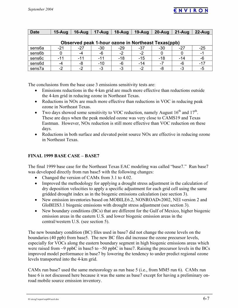
September 2004
H:\etcog3\report\sept04\sec6.doc 6-7
Date 15-Aug 16-Aug 17-Aug 18-Aug 19-Aug 20-Aug 21-Aug 22-Aug
Observed peak 1-hour ozone in Northeast Texas(ppb) sens6a -21 -27 -30 -29 -37 -30 -27 -25 sens6b 0 -4 -6 -2 -2 0 0 -1 sens6c -11 -11 -11 -18 -15 -18 -14 -6 sens6d -4 -8 -10 -6 -14 -7 -6 -17 sens7a -2 -2 -3 -3 -2 -8 -3 -5
The conclusions from the base case 3 emissions sensitivity tests are:
• Emissions reductions in the 4-km grid are much more effective than reductions outside the 4-km grid in reducing ozone in Northeast Texas.
• Reductions in NOx are much more effective than reductions in VOC in reducing peak ozone in Northeast Texas.
• Two days showed some sensitivity to VOC reduction, namely August 16th and 17th. These are days when the peak modeled ozone was very close to CAMS19 and Texas Eastman. However, NOx reduction is still more effective than VOC reduction on these days.
• Reductions in both surface and elevated point source NOx are effective in reducing ozone in Northeast Texas.
FINAL 1999 BASE CASE – BASE7 The final 1999 base case for the Northeast Texas EAC modeling was called “base7.” Run base7 was developed directly from run base5 with the following changes:
• Changed the version of CAMx from 3.1 to 4.02. • Improved the methodology for applying a drought stress adjustment in the calculation of
dry deposition velocities to apply a specific adjustment for each grid cell using the same gridded drought index as in the biogenic emissions calculation (see section 3).
• New emission inventories based on MOBILE6.2, NONROADv2002, NEI version 2 and GloBEIS3.1 biogenic emissions with drought stress adjustment (see section 3).
• New boundary conditions (BCs) that are different for the Gulf of Mexico, higher biogenic emission areas in the eastern U.S. and lower biogenic emission areas in the central/western U.S. (see section 5).
The new boundary condition (BC) files used in base7 did not change the ozone levels on the boundaries (40 ppb) from base5. The new BC files did increase the ozone precursor levels, especially for VOCs along the eastern boundary segment in high biogenic emissions areas which were raised from ~9 ppbC in base5 to ~50 ppbC in base7. Raising the precursor levels in the BCs improved model performance in base7 by lowering the tendency to under predict regional ozone levels transported into the 4-km grid. CAMx run base7 used the same meteorology as run base 5 (i.e., from MM5 run 6). CAMx run base 6 is not discussed here because it was the same as base7 except for having a preliminary on-road mobile source emission inventory.

September 2004
H:\etcog3\report\sept04\sec6.doc 6-8
MODEL PERFORMANCE EVALUATION The performance of the ozone modeling for 15-22 August 1999 was evaluated according to EPA’s draft guidance for 8-hour ozone modeling (EPA, 1999). This guidance suggests several methods that can be used to evaluate the performance of air quality models and in some cases suggest performance goals. In general, the draft 8-hour guidance differs from earlier EPA modeling guidance by encouraging use of a variety of evaluation methods to seek good performance for the right reasons as opposed to establishing a few rigid criteria. NETAC used several graphical and statistical methods to evaluate performance as listed below. Graphical Performance Evaluation Methods:
• Isopleth plots of predictions and observations • Time-series plots of predictions and observations • Scatter plots of predictions and observations • Quantile-quantile (Q-Q) plots of predictions and observations
Statistical Performance Evaluation Methods:
• Normalized bias for prediction/observation pairs (goal within 15%) • Fractional bias for prediction/observation pairs • Normalized gross error predictions and observations (goal within 35%) • Fractional gross error predictions and observations • Peak prediction and observation (goal within 20%) • Correlation coefficient from prediction/observation scatter plots (goal moderate to large
positive correlations) • Bias in predicted/observed daily maximum near each monitor (goal within 20% at most
monitors). The bias and error statistical measures are defined as follows:
Where Otl and Etl are, respectively, the observed and estimated ozone concentration at site l and time t (i.e., matched by time and location).
( )Normalized Bias 1001N
E O /Otl tl tl=
−∑
Normalized Gross Error 1001N
E O /Otl tl tl=
−∑
( ) ( )Fractional Bias 1001N
E -O / E +Otl tl tl tl=
∑ 2
( )Fractional Gross Error 1001N
E O / E Otl tl tl tl=
− +∑ 2

September 2004
H:\etcog3\report\sept04\sec6.doc 6-9
Graphical Evaluation Modeled daily maximum 8-hour ozone levels for the regional 12-km grid are shown for August 17th by the colored shading in Figure 6-1. This day is at the heart of the ozone episode in Northeast Texas and the figure shows high ozone levels covering northern Texas, northern Louisiana and southern Arkansas due to regional weather stagnation. The highest modeled ozone levels are in Northeast Texas because this is near the center of the stagnation allowing local anthropogenic and biogenic emissions to interact under conditions that are conducive to ozone formation. Ozone production within Northeast Texas combined with the regional background lead to the high ozone levels modeled in the region on August 17th and following days. This pattern is consistent with the conceptual model for high 8-hour ozone episodes in Northeast Texas in general and the 15-22 August 1999 ozone episode in particular. Similar figures for other episode days are included in Appendix B. The modeled and observed daily maximum 8-hour ozone levels for the 4-km grid are shown in Figure 6-2 for the 16th, 17th, 18th and 22nd August 1999 (other days are included in Appendix A). The colored shading shows the modeled ozone and monitored values are shown as numbers. The model has a tendency to under predict the observed maximum ozone levels on August 16th at both the upwind monitors (Cypress River and Shreveport) and Longview/Tyler suggesting the background ozone transported into Northeast Texas may be too low in the model. The modeled and observed ozone levels agree better on August 17th and 18th when the modeling does not tend to under predict ozone. On August 22nd the modeled maximum ozone levels at Tyler and Longview agree well with the observed values but at the upwind monitors (Cypress River and Shreveport) the modeling under predicts the maximum ozone levels again suggesting that the background ozone transported into Northeast Texas may be too low in the model.
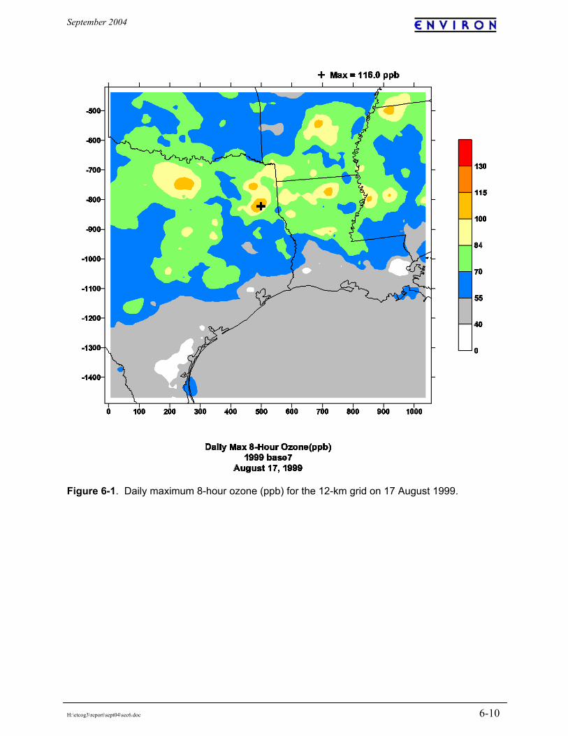
September 2004
H:\etcog3\report\sept04\sec6.doc 6-10
Figure 6-1. Daily maximum 8-hour ozone (ppb) for the 12-km grid on 17 August 1999.

September 2004
H:\etcog3\report\sept04\sec6.doc 6-11
16 August 1999 17 August 1999
18 August 1999
22 August 1999
Figure 6-2. Daily maximum 8-hour ozone (ppb) for the 4-km grid.

September 2004
H:\etcog3\report\sept04\sec6.doc 6-12
The model performance features for the 4-km grid discussed above also are shown in the time series of 8-hour ozone shown in Figure 6-3. In addition, the time series show that the model performs well in predicting the timing of the daily peak ozone levels. The largest differences in the time series occur at night, especially at the rural Cypress River monitor during the heart of the episode. These differences are not problematic since it can be difficult to obtain good nighttime model performance because limited atmospheric mixing at night means that monitors can be influenced by localized conditions that are not resolved at 4-km grid resolution. Time series of 1-hour ozone are included in Appendix E for the 12-km grid and Appendix F for the 4-km grid.
Figure 6-3. Time series of 8-hour ozone (ppb) for monitors in Northeast Texas. Statistical Evaluation Several model performance statistics were calculated from the data shown in Figure 6-3 for monitors in Northeast Texas and the statistical measures are shown in Table 6-5. The normalized bias indicates whether there was a tendency to over or under predict observed ozone concentrations greater than 60 ppb at monitor locations on each day. There is an under prediction bias on all days except August 18th but the bias is within the EPA goal on 6 of 8 days. The accuracy of the peak indicates whether there was a tendency to over or under predict the highest observed ozone concentrations on each day. The observed peak was over predicted on 6 of 8 days and was outside the EPA goal of 20% on two days. Taken together with the conclusions from the Figure 6-3 isopleth plots discussed above, these results indicate that the negative bias results from too little ozone transport into Northeast Texas rather than a lack of local ozone production. The normalized gross error describes the level of agreement between the modeled and observed ozone at the monitor locations and the gross error values shown in Table 6-5 are well within the EPA performance goal on all days.
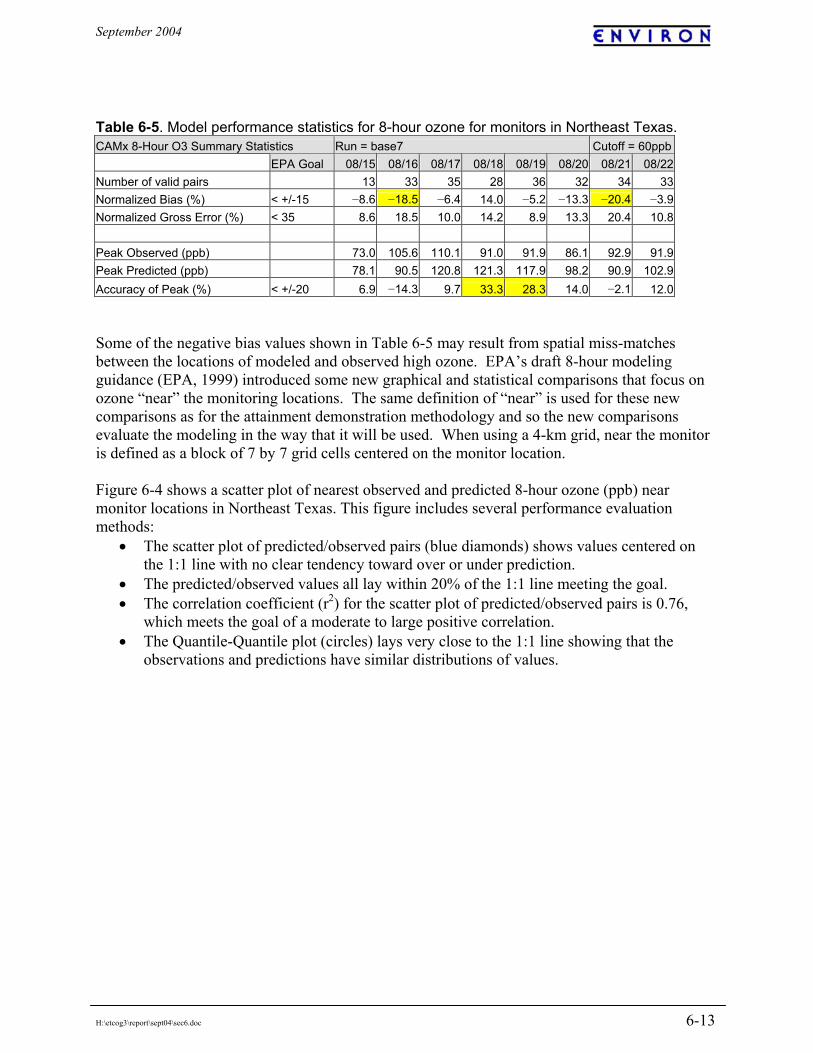
September 2004
H:\etcog3\report\sept04\sec6.doc 6-13
Table 6-5. Model performance statistics for 8-hour ozone for monitors in Northeast Texas. CAMx 8-Hour O3 Summary Statistics Run = base7 Cutoff = 60ppb EPA Goal 08/15 08/16 08/17 08/18 08/19 08/20 08/21 08/22Number of valid pairs 13 33 35 28 36 32 34 33Normalized Bias (%) < +/-15 −8.6 −18.5 −6.4 14.0 −5.2 −13.3 −20.4 −3.9Normalized Gross Error (%) < 35 8.6 18.5 10.0 14.2 8.9 13.3 20.4 10.8 Peak Observed (ppb) 73.0 105.6 110.1 91.0 91.9 86.1 92.9 91.9Peak Predicted (ppb) 78.1 90.5 120.8 121.3 117.9 98.2 90.9 102.9Accuracy of Peak (%) < +/-20 6.9 −14.3 9.7 33.3 28.3 14.0 −2.1 12.0 Some of the negative bias values shown in Table 6-5 may result from spatial miss-matches between the locations of modeled and observed high ozone. EPA’s draft 8-hour modeling guidance (EPA, 1999) introduced some new graphical and statistical comparisons that focus on ozone “near” the monitoring locations. The same definition of “near” is used for these new comparisons as for the attainment demonstration methodology and so the new comparisons evaluate the modeling in the way that it will be used. When using a 4-km grid, near the monitor is defined as a block of 7 by 7 grid cells centered on the monitor location. Figure 6-4 shows a scatter plot of nearest observed and predicted 8-hour ozone (ppb) near monitor locations in Northeast Texas. This figure includes several performance evaluation methods:
• The scatter plot of predicted/observed pairs (blue diamonds) shows values centered on the 1:1 line with no clear tendency toward over or under prediction.
• The predicted/observed values all lay within 20% of the 1:1 line meeting the goal. • The correlation coefficient (r2) for the scatter plot of predicted/observed pairs is 0.76,
which meets the goal of a moderate to large positive correlation. • The Quantile-Quantile plot (circles) lays very close to the 1:1 line showing that the
observations and predictions have similar distributions of values.

September 2004
H:\etcog3\report\sept04\sec6.doc 6-14
Figure 6-4. Scatter plot of nearest observed and predicted 8-hour ozone (ppb) near monitor locations in Northeast Texas. Quantiles are also shown as circles and the dashed lines show +/- 20% bias. The r2 value is the correlation coefficient. Conclusions on Model Performance The model performance evaluation results presented and discussed above show that the perception of model performance depends upon the methodology used for evaluation. Therefore, it is important to look at the model performance evaluation as a whole and seek to determine whether the model is suitable for use in the intended purpose of an 8-hour ozone attainment demonstration. Overall conclusions from the performance evaluation are:
• Modeled ozone formation is consistent with conceptual model in showing that high ozone levels in Northeast Texas resulted from a combination of production from local emissions sources combined with a regional background and transport of ozone.
• There is some evidence for ozone under prediction near the beginning and end of the episodes and this appears to result from the model having too low ozone transport into Northeast Texas from the east and northeast.
• Model performance is acceptable on most days when evaluated using the more traditional methods developed for 1-hour ozone modeling (such as the normalized bias).
• Model performance is very good when evaluated using newer methods developed in EPA’s draft modeling guidance (EPA, 1999) that compare ozone levels near monitor locations and better correspond to the 8-hour ozone attainment demonstration methodology.

September 2004
H:\etcog3\report\sept04\sec6.doc 6-15
The overall conclusion is that the ozone modeling is suitable for use in an 8-hour ozone attainment demonstration for Northeast Texas. MODELING PROCEDURES FOR 2002 AND 2007 The purpose of the future year ozone modeling is to project whether Northeast Texas will be attaining the 8-hour ozone standard in 2007. This analysis is referred to as an “attainment demonstration” based on ozone modeling. The attainment demonstration depends upon changes in modeled ozone levels between a base and a future year and so it is important that the base and future year modeling be as consistent as possible. The objective is to ensure that modeled ozone changes between the base and future year result from emissions changes and therefore provide an accurate and realistic estimate of the ozone changes that will occur in Northeast Texas. As discussed in detail below, the attainment demonstration relied upon changes in modeled ozone levels between a base year of 2002 and a future year of 2007. The only difference between the modeling for 1999, 2002 and 2007 was in the anthropogenic emissions inputs to the CAMx model as described in section 3. Specifically, between years there were:
• No changes to the CAMx model (version 4.02). • No changes to the CAMx model options. • No changes to the meteorological input files. • No changes to the initial and boundary conditions. • No changes to the biogenic emissions.
With these modeling methods and assumptions all changes in ozone levels between modeled years are due solely to the effects of emissions growth and controls. The emission inventory development was described above in section 3 and the emissions control measures assumed to be in place for 2007 are described next. The final 2002 base case model run was called “02base3” and the final 2007 model run was called “07base5.” Modeled ozone levels in the 4-km grid are shown for 2002 in Appendix C and for 2007 in Appendix D. The changes in modeled ozone levels from 1999 to 2002 to 2007 and their relationship to emissions changes were investigated using the ozone source apportionment technology (OSAT) option in CAMx, as described in section 7. EMISSION CONTROLS FOR 2007 The 2007 emission inventories rely upon emission control measures that are currently enforceable. These measures are a combination of Federal measures developed by EPA, State measures developed by Texas for the State Implementation Plan (SIP) and local measures developed by NETAC that have been made enforceable by agreed orders.

September 2004
H:\etcog3\report\sept04\sec6.doc 6-16
On-road Mobile Sources The following federal emission reduction programs for on-road vehicles were accounted for using EPA’s MOBILE6 model:
• Tier 1 light-duty vehicle standards, beginning with the 1996 model year • National Low Emission Vehicle (NLEV) standards for light-duty vehicles, beginning
with model year 2001 • Tier 2 light-duty vehicle standards, beginning with model year 2005, with low sulfur
gasoline beginning in the summer of 2004 • Heavy-duty vehicle standards, beginning with model year 2004 • Heavy-duty vehicle standards (with low sulfur diesel), beginning with model year 2007.
Off-road Mobile Sources The following federal emission reduction programs for off-road vehicles were accounted for using EPA’s NONROAD model:
• Phase 1 and 2 emission standards for new off-road spark-ignition engines at or below 25 horsepower (hp). Different starts and phase-in periods depending on engine size. Earliest start year is 1997 model year.
• Emission standards for new gasoline spark-ignition marine engines. Phase-in starts with 1998 model year.
• Tier 1 and Tier 2 emission standards for new off-road compression-ignition engines below 50 hp, including recreational marine engines less than 50 hp. Phase-in period differs by Tier and engine size. Earliest start year is 1997 model year.
• Tier 1 through Tier 3 emission standards for new off-road compression-ignition engines at or above 50 hp, not including recreational marine engines greater than 50 hp. Phase-in period differs by Tier and engine size. Earliest start year is 1996 model year.
Emissions from aircraft, commercial marine and locomotives are estimated outside of the NONROAD model. Commercial marine emissions in the NETAC area are negligible. No emission controls were assumed for aircraft. Locomotive emissions were adjusted to account for EPA regulations promulgated in 1997. Stationary Sources The impact of control programs on stationary sources was modeled separately for Northeast Texas, the rest of Texas and States outside Texas. For stationary (area and point) sources outside of Texas, the 2007 anthropogenic emission inventories were the modeling inventories developed by EPA for a rulemaking on “heavy duty diesel” emissions and include EPA’s estimates of emission reductions including the NOx SIP Call. For area and point sources within Texas, the 2007 emission inventory includes reductions due to all of the TCEQ’s State Implementation Plans (SIPs) for the non-attainment areas (Houston-Galveston, Beaumont-Port Arthur, Dallas/Fort Worth) and other areas as published in the Texas Administrative Code (Coulter-Burke et al., 2002). In some cases this tends to under-state the

September 2004
H:\etcog3\report\sept04\sec6.doc 6-17
emission reductions because some SIP strategies have yet to be published as rules in the Texas Administrative Code. Major Point Sources in Northeast Texas Emissions at several major point sources in Northeast Texas were reduced to reflect control measures implemented in the 1-hour ozone SIP for Northeast Texas adopted by the TCEQ on March 13, 2002. This SIP includes NOx emission reductions from utility sources operated by American Electric Power (AEP) and Texas Utilities (TXU), as well as NOx emission reductions at Eastman Chemical Company, Texas operations (Eastman). These local reductions were developed voluntarily through NETAC and made enforceable through agreed orders. The NOx emissions for the utility sources affected by NETAC local controls were estimated by multiplying the permit limit emission factors (lb NOx/mmBtu) by heat input values (mmBtu/hour) from a July 1997 ozone episode period. This is the same methodology (and therefore the same emissions) as used in the 1-hour ozone SIP modeling for Northeast Texas (TNRCC, 2002). The resulting daily emission rates and the reductions due to controls in 2007 are shown in Tables 6-6 and 6-7. The dates when these controls were implemented differed by facility as shown in Table 6-8. Most of the reductions in NOx emissions at major point sources in Northeast Texas were implemented by 2002 and, with the exception of one unit, all were implemented by the 2003 ozone season. Table 6-6. Reductions in AEP 2007 NOx emissions due to NETAC local controls.
2007 Base Case 2007 Strategy Reduction Facility lb/mmBtu ton/day lb/mmBtu ton/day ton/day Percent
Wilkes Unit 1 N/A 1.5 N/A 1.5 0.0 0% Unit 2 0.31 5.3 0.17 2.9 2.4 45% Unit 3 0.38 5.8 0.17 2.6 3.2 55% All units 12.6 7.0 5.6 44% Knox Lee Unit 2 N/A 0.3 N/A 0.3 0.0 0% Unit 3 N/A 0.3 N/A 0.3 0.0 0% Unit 4 N/A 2.1 N/A 2.1 0.0 0% Unit 5 0.24 4.4 0.18 3.2 1.1 26% All units 7.1 6.0 1.1 16% Pirkey 0.31 25.4 0.22 17.9 7.5 29% Note: N/A = information not available
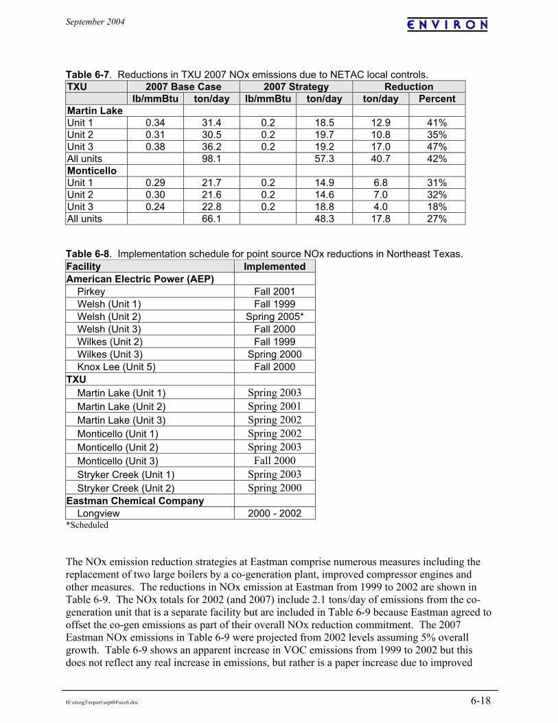
September 2004
H:\etcog3\report\sept04\sec6.doc 6-18
Table 6-7. Reductions in TXU 2007 NOx emissions due to NETAC local controls. TXU 2007 Base Case 2007 Strategy Reduction
lb/mmBtu ton/day lb/mmBtu ton/day ton/day Percent Martin Lake Unit 1 0.34 31.4 0.2 18.5 12.9 41% Unit 2 0.31 30.5 0.2 19.7 10.8 35% Unit 3 0.38 36.2 0.2 19.2 17.0 47% All units 98.1 57.3 40.7 42% Monticello Unit 1 0.29 21.7 0.2 14.9 6.8 31% Unit 2 0.30 21.6 0.2 14.6 7.0 32% Unit 3 0.24 22.8 0.2 18.8 4.0 18% All units 66.1 48.3 17.8 27% Table 6-8. Implementation schedule for point source NOx reductions in Northeast Texas. Facility Implemented American Electric Power (AEP) Pirkey Fall 2001 Welsh (Unit 1) Fall 1999 Welsh (Unit 2) Spring 2005* Welsh (Unit 3) Fall 2000 Wilkes (Unit 2) Fall 1999 Wilkes (Unit 3) Spring 2000 Knox Lee (Unit 5) Fall 2000 TXU Martin Lake (Unit 1) Spring 2003 Martin Lake (Unit 2) Spring 2001 Martin Lake (Unit 3) Spring 2002 Monticello (Unit 1) Spring 2002 Monticello (Unit 2) Spring 2003 Monticello (Unit 3) Fall 2000 Stryker Creek (Unit 1) Spring 2003 Stryker Creek (Unit 2) Spring 2000 Eastman Chemical Company Longview 2000 - 2002 *Scheduled The NOx emission reduction strategies at Eastman comprise numerous measures including the replacement of two large boilers by a co-generation plant, improved compressor engines and other measures. The reductions in NOx emission at Eastman from 1999 to 2002 are shown in Table 6-9. The NOx totals for 2002 (and 2007) include 2.1 tons/day of emissions from the co-generation unit that is a separate facility but are included in Table 6-9 because Eastman agreed to offset the co-gen emissions as part of their overall NOx reduction commitment. The 2007 Eastman NOx emissions in Table 6-9 were projected from 2002 levels assuming 5% overall growth. Table 6-9 shows an apparent increase in VOC emissions from 1999 to 2002 but this does not reflect any real increase in emissions, but rather is a paper increase due to improved
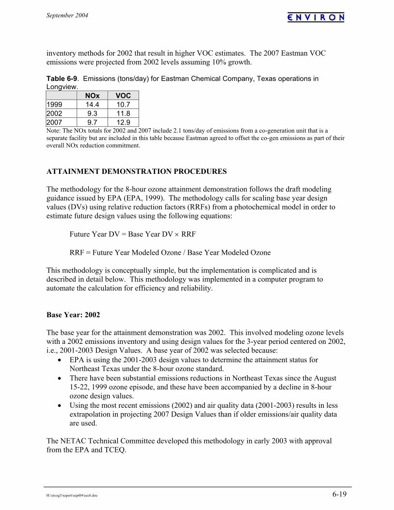
September 2004
H:\etcog3\report\sept04\sec6.doc 6-19
inventory methods for 2002 that result in higher VOC estimates. The 2007 Eastman VOC emissions were projected from 2002 levels assuming 10% growth. Table 6-9. Emissions (tons/day) for Eastman Chemical Company, Texas operations in Longview. NOx VOC 1999 14.4 10.7 2002 9.3 11.8 2007 9.7 12.9 Note: The NOx totals for 2002 and 2007 include 2.1 tons/day of emissions from a co-generation unit that is a separate facility but are included in this table because Eastman agreed to offset the co-gen emissions as part of their overall NOx reduction commitment. ATTAINMENT DEMONSTRATION PROCEDURES The methodology for the 8-hour ozone attainment demonstration follows the draft modeling guidance issued by EPA (EPA, 1999). The methodology calls for scaling base year design values (DVs) using relative reduction factors (RRFs) from a photochemical model in order to estimate future design values using the following equations: Future Year DV = Base Year DV × RRF RRF = Future Year Modeled Ozone / Base Year Modeled Ozone This methodology is conceptually simple, but the implementation is complicated and is described in detail below. This methodology was implemented in a computer program to automate the calculation for efficiency and reliability. Base Year: 2002 The base year for the attainment demonstration was 2002. This involved modeling ozone levels with a 2002 emissions inventory and using design values for the 3-year period centered on 2002, i.e., 2001-2003 Design Values. A base year of 2002 was selected because:
• EPA is using the 2001-2003 design values to determine the attainment status for Northeast Texas under the 8-hour ozone standard.
• There have been substantial emissions reductions in Northeast Texas since the August 15-22, 1999 ozone episode, and these have been accompanied by a decline in 8-hour ozone design values.
• Using the most recent emissions (2002) and air quality data (2001-2003) results in less extrapolation in projecting 2007 Design Values than if older emissions/air quality data are used.
The NETAC Technical Committee developed this methodology in early 2003 with approval from the EPA and TCEQ.
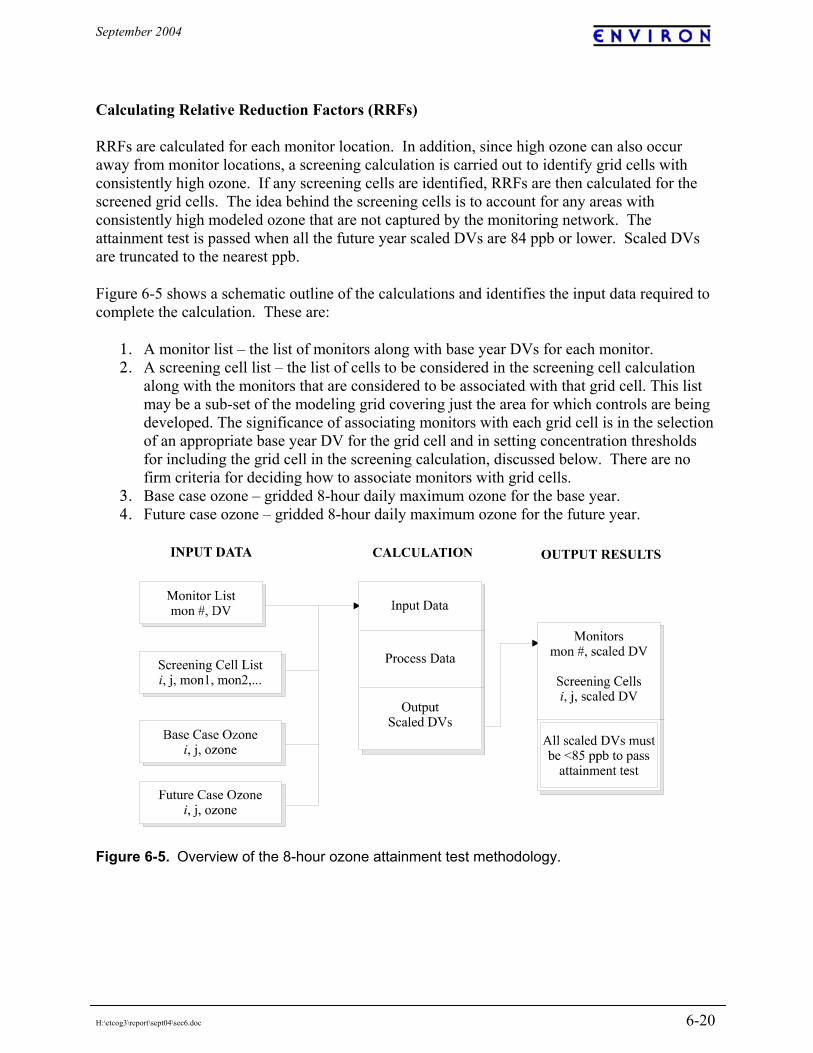
September 2004
H:\etcog3\report\sept04\sec6.doc 6-20
Calculating Relative Reduction Factors (RRFs) RRFs are calculated for each monitor location. In addition, since high ozone can also occur away from monitor locations, a screening calculation is carried out to identify grid cells with consistently high ozone. If any screening cells are identified, RRFs are then calculated for the screened grid cells. The idea behind the screening cells is to account for any areas with consistently high modeled ozone that are not captured by the monitoring network. The attainment test is passed when all the future year scaled DVs are 84 ppb or lower. Scaled DVs are truncated to the nearest ppb. Figure 6-5 shows a schematic outline of the calculations and identifies the input data required to complete the calculation. These are:
1. A monitor list – the list of monitors along with base year DVs for each monitor. 2. A screening cell list – the list of cells to be considered in the screening cell calculation
along with the monitors that are considered to be associated with that grid cell. This list may be a sub-set of the modeling grid covering just the area for which controls are being developed. The significance of associating monitors with each grid cell is in the selection of an appropriate base year DV for the grid cell and in setting concentration thresholds for including the grid cell in the screening calculation, discussed below. There are no firm criteria for deciding how to associate monitors with grid cells.
3. Base case ozone – gridded 8-hour daily maximum ozone for the base year. 4. Future case ozone – gridded 8-hour daily maximum ozone for the future year.
Figure 6-5. Overview of the 8-hour ozone attainment test methodology.

September 2004
H:\etcog3\report\sept04\sec6.doc 6-21
The details of the calculations are as follows: • Monitor DV Scaling
1. For each monitor, find the daily maximum 8-hour ozone in an n x n block of cells around the monitor for both the base and future case. Repeat for each modeling day being used for control strategy development. For a 4 km grid, n=7 according to the guidance.
2. Exclude days when the base case daily maximum 8-hour ozone was below 70 ppb. 3. Average the daily maximum 8-hour ozone across days for the base and future year. 4. Calculate the RRF = (average future daily max) / (average base daily max). 5. Calculate the scaled DV = base year DV x RRF. 6. Repeat 1-5 for each monitor
• Screening Cell DV Scaling
7. For each grid cell on the screening cell list, count the number of days where the modeled daily maximum 8-hour ozone is at least 5% greater than the modeled daily maximum 8-hour ozone at any “associated” monitor, and at least 70 ppb.
8. If the number of days is 50% or greater of the total days, treat this cell as if it were a monitor – this is a “screened cell.”
9. The base year DV to be used for a screened cell is the maximum of the base year DVs for any “associated” monitor.
10. Calculated the scaled DV for each screened cell as if it were a monitor (steps 1-5 above). 11. Repeat 7-10 for each grid cell on the screening cell list.
ATTAINMENT DEMONSTRATION The EPA design value scaling methodology was applied for all ozone monitoring locations in Northeast Texas in 2003. The screening cell methodology described above identified no screening cells to be considered in addition to the monitor locations. The Longview and Tyler monitors have full 2001-2003 DVs whereas the Karnack and Waskom monitors have 2-year (2002-2003) DVs. The RRFs at all four monitor locations are less than 1.0 showing that modeled ozone levels across Northeast Texas decreased from 2002 to 2007. Table 6-10. Projected 2007 8-hour ozone design values (DV; ppb) for Northeast Texas ozone monitor locations in 2003. Monitor
Preliminary 2003 Design Value
Modeled Relative Reduction Factor
Projected 2007 Design Value
Longview 82 0.981 80 Tyler 81 0.954 77 Karnack 84 0.966 81 Waskom 84 0.974 82
Notes: 2003 DVs are based on preliminary 2003 monitoring data. The Longview and Tyler monitors have 2001-2003 DVs. The Karnack and Waskom monitors have 2002-2003 DVs.

September 2004
H:\etcog3\report\sept04\sec6.doc 6-22
The ozone modeling demonstrates attainment of the 8-hour ozone standard in 2007 because the projected 2007 DVs shown in Table 6-10 are all less than 84 ppb. As discussed above, the 2007 control strategy relies entirely upon measures that are already enforceable including substantial NOx reductions at local point sources developed by NETAC. NETAC is continuing to develop additional local reductions for Northeast Texas. The conclusion based on modeling that Northeast Texas will continue to demonstrate attainment of the 8-hour ozone standard in 2007 is conservative in several ways:
• The projected 2007 8-hour ozone levels at Longview and Tyler are 4 and 7 ppb below the highest level that would demonstrate attainment (84 ppb) providing a margin of safety.
• Additional emissions reductions beyond those assumed in the modeling are expected to occur by 2007.
• The relative reduction factors used to project the 2007 design values depend upon ratios of 2007 to 2002 modeled ozone levels. The utility emission estimates for 2007 are more conservative than for 2002 (permit maximum rather than summer average levels, see section 3) which introduces a bias toward higher projected 2007 ozone levels.
WEIGHT-OF-EVIDENCE SUPPORTING THE ATTAINMENT DEMONSTRATION This section considers whether the weight-of-evidence supports the conclusions from the ozone modeling that ozone levels in Northeast Texas will continue to decline and that consequently the area will move further into compliance with the 8-hour ozone standard by 2007. Given that the ozone control strategy for Northeast Texas focuses on NOx reductions, the weight-of-evidence analysis considers three factors:
1. Evidence that ozone levels in Northeast Texas will respond to reductions in NOx emissions.
2. Trends in NOx emissions. 3. Ozone trends as NOx reductions have been implemented in recent years.
The conceptual model completed by Stoeckenius et al. (2004) considered whether ozone levels are expected to be more responsive to NOx or VOC reductions and concluded that ozone production in Northeast Texas is expected to be NOx limited. This conclusion was based on the high VOC:NOx ratio (greater than 30) in the emission inventory which is well within the NOx-limited regime. The high VOC:NOx ratio results from high biogenic emission levels which are generally considered to lead to NOx-limited ozone formation in forested, predominantly rural areas like Northeast Texas. Emissions sensitivity tests using the August 1999 ozone model (discussed above) also showed that NOx reductions were the most effective way of reducing ozone. Therefore, the weight-of-evidence suggests that ozone will respond to NOx reductions. The trends in NOx emissions from 1999 to 2012 were by Stoeckenius et al., (2004) and are shown in Figure 6-6. This analysis showed that total anthropogenic NOx emissions decrease consistently from 1999 to 2012 due primarily to decreases in point source NOx in the early years and decreases in mobile source NOx in the later years. The decreases in NOx emissions from 1999 levels were:
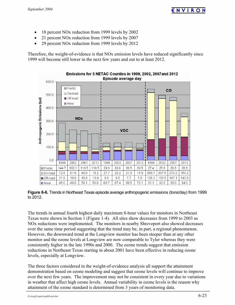
September 2004
H:\etcog3\report\sept04\sec6.doc 6-23
• 18 percent NOx reduction from 1999 levels by 2002 • 21 percent NOx reduction from 1999 levels by 2007 • 29 percent NOx reduction from 1999 levels by 2012
Therefore, the weight-of-evidence is that NOx emission levels have reduced significantly since 1999 will become still lower in the next few years and out to at least 2012.
Figure 6-6. Trends in Northeast Texas episode average anthropogenic emissions (tons/day) from 1999 to 2012. The trends in annual fourth highest daily maximum 8-hour values for monitors in Northeast Texas were shown in Section 1 (Figure 1-4). All sites show decreases from 1999 to 2003 as NOx reductions were implemented. The monitors in nearby Shreveport also showed decreases over the same time period suggesting that the trend may be, in part, a regional phenomenon. However, the downward trend at the Longview monitor has been steeper than at any other monitor and the ozone levels at Longview are now comparable to Tyler whereas they were consistently higher in the late 1990s and 2000. The ozone trends suggest that emission reductions in Northeast Texas starting in about 2001 have been effective in reducing ozone levels, especially at Longview. The three factors considered in the weight-of-evidence analysis all support the attainment demonstration based on ozone modeling and suggest that ozone levels will continue to improve over the next few years. The improvement may not be consistent in every year due to variations in weather that affect high ozone levels. Annual variability in ozone levels is the reason why attainment of the ozone standard is determined from 3 years of monitoring data.

September 2004
H:\etcog3\report\sept04\sec7.doc 7-1
7. SOURCE CONTRIBUTIONS TO OZONE One of the unique features of CAMx is the availability of several “probing tools” to provide additional diagnostic and sensitivity information for an ozone simulation. The probing tools can be used to answer questions such as:
• Which emissions cause high ozone? • How will ozone levels respond to emission changes? • How important are the initial and boundary conditions? • What are the influences of different model processes (chemistry, deposition, etc.) on
ozone levels at a specific location?
The probing tools can also provide information for ozone precursors. The tools that are available have differing capabilities and uses. This section briefly describes the available probing tools and then presents results from the application of ozone source apportionment to the 1999, 2002 and 2007 base case simulations for Northeast Texas. SUMMARY OF CAMx PROBING TOOLS The probing tools available in version 4.0 of CAMx are:
• Ozone Source Apportionment Technology (OSAT) and related methods (APCA). • The Decoupled Direct Method (DDM) for sensitivity analysis. • Process Analysis.
OSAT provides information about the relationships between ozone concentrations and sources of precursors in the form of ozone source apportionments. Source apportionment means that the sum of the source contributions adds up to exactly 100% of the total ozone and so all of the ozone is accounted for. OSAT attributes ozone among all of the potential sources of ozone in the simulation, namely emissions, boundary conditions and initial conditions. Ozone formation from VOC and NOx precursors is tracked separately. The emissions contributions can be broken down by geographic area and/or source category. The OSAT methods are described in the CAMx User’s Guide (ENVIRON, 2004) and in Dunker et al., (2002b). Because ozone formation chemistry is a non-linear process, there is no unique way of apportioning ozone back to precursor sources. The OSAT methods attribute ozone formation to precursors that were present at the time the ozone was formed. There are two schemes for doing this called OSAT and APCA. The OSAT or APCA results are just like any other ozone source apportionment in that they are not exact. However, OSAT and APCA are very helpful for estimating the relative importance of different sources and guiding control strategy development. The difference between the OSAT and APCA schemes can be summarized as follows. OSAT apportions ozone formation based solely on what precursors were present when the ozone is formed. OSAT determines whether ozone formation is NOx or VOC limited in each grid cell at each time step, and attributes ozone production according to the relative contributions of the limiting precursor (VOC or NOx) from different sources present at that time. APCA modifies

September 2004
H:\etcog3\report\sept04\sec7.doc 7-2
the OSAT method to account for the fact that biogenic emissions are not considered to be controllable, and therefore attributes ozone to controllable (anthropogenic) emissions whenever possible. The differences between OSAT and APCA are discussed in more detail below. The DDM provides similar types of information to OSAT, but in terms of sensitivity coefficients rather than source apportionments. Sensitivity coefficients describe how ozone will change if a precursor source is changed and thus are useful for predicting the effects of control strategies. CAMx can calculate “first-order” sensitivity coefficients, which are the likely to be the most important sensitivities, and are somewhat similar to source apportionments. There are two major differences between DDM sensitivities and OSAT source apportionments: (1) Sensitivity coefficients can be negative, meaning that reducing emissions will increase ozone, whereas as source apportionments are never negative. An example would be an area with high NOx emissions where reducing NOx emissions will increase ozone and DDM will obtain negative ozone sensitivities to local NOx whereas OSAT will have zero or small ozone apportionments to local NOx. (2) Adding up all the first-order sensitivities over all sources of ozone and precursors usually explains only about 60% of the total ozone. The modeled ozone that is “unexplained” by the first-order sensitivity coefficients can be explained by higher-order sensitivities, but they are more difficult to calculate and difficult to interpret. An advantage of DDM sensitivity coefficients is that they are rigorously defined (mathematically) and so are unique. The value of this uniqueness is weakened if the sensitivities are interpreted as source apportionments because of the significant portion of the ozone that is “unexplained” by the first-order sensitivities. Further information on DDM is provided in Dunker et al. (2002 a and b) and the CAMx User’s Guide (ENVIRON, 2004). Process analysis (PA) is a method for obtaining more information on how CAMx predicted concentrations at a specific place and time. The CAMx concentrations are determined by numerous model processes (such as emissions, transport, chemistry, deposition) but the separate contribution of each process is hidden within the final concentration output. Process analysis allows the contribution of each process to be output and used in diagnostic analyses. This is useful for explaining “how the model got the answer it got” and thus understanding model performance issues. Process analysis is not well suited for understanding source contributions to ozone or predicting responses to emissions changes. Further information on process analysis is provided in the CAMx User’s Guide (ENVIRON, 2004) and references therein. Anthropogenic Precursor Culpability Assessment (APCA) Applications of OSAT to the Eastern US consistently identify biogenic emissions as a major contributor to ozone formation. This is not surprising as biogenic VOC emissions are very reactive and dominate regional VOC emissions in the Eastern US, but this finding is not “policy relevant” for designing anthropogenic emissions ozone control plans. The APCA methodology was developed from OSAT to address this issue. APCA stands for Anthropogenic Precursor Culpability Assessment, and differs from OSAT in recognizing that certain emission groups are not controllable (i.e., biogenic emissions) and that apportioning ozone production to these emissions does not provide control strategy relevant information. To address this, in situations where OSAT attributes ozone formation to a non-controllable source category when it was due to the interaction of ozone precursors from a non-controllable (i.e., biogenic) and controllable emissions source, APCA re-directs the ozone attribution to the controllable precursor. In practice, biogenic emissions are the uncontrollable source category and APCA only attributes

September 2004
H:\etcog3\report\sept04\sec7.doc 7-3
ozone production to biogenic emissions when ozone formation is due to the interaction of biogenic VOC with biogenic NOx. When ozone formation is due to biogenic VOC interacting with anthropogenic NOx under VOC-limited conditions (where OSAT would attribute ozone production to biogenic VOC’s), APCA directs the attribution to the anthropogenic NOx precursors present. The result of using APCA instead of OSAT is that more ozone formation is attributed to anthropogenic NOx sources and little ozone formation is attributed to biogenic sources. APCA is not called a “source apportionment” technique because it expresses biases as to which sources should be implicated (i.e., those that are controllable), hence it is referred to as a “culpability assessment.” STRENGTHS AND LIMITATIONS OF OSAT AND APCA The main advantage of OSAT and APCA is providing a clear apportionment of ozone concentrations among all of the sources of ozone precursors in CAMx. These precursor sources (emissions, boundary conditions and initial conditions) can be sub-divided into categories to provide refined analyses. For example the emissions can be sub-divided based on emissions category and/or geographic area. This information provides a clear understanding of which sources are involved in forming the ozone present at a specific place and time. The apportionments are based on the participation of precursor emissions in the ozone formation process. The main limitation of OSAT and APCA is that, because ozone formation is not a linear process, the source contributions cannot be used to exactly calculate what emission reductions are needed to achieve a specific target ozone level. As ozone precursor emissions are reduced, the efficiency of ozone formation changes and controls may become more or less effective than expected. Thus, OSAT and APCA should be used as a guide for designing control strategies, but can not provide an exact control strategy solution. SOURCE APPORTIONMENT ANALYSIS DESIGN The OSAT and APCA probing tools were used for the source apportionment analyses. The APCA results are expected to be more useful because of the high contribution biogenic emissions in Northeast Texas. Emissions were divided into 4 source categories and 10 geographic areas as defined in Tables 7-1 and 7-2, respectively. The source areas are also shown as maps for the 36-km, 12-km and 4-km CAMx grids in Figure 7-1. This means that ozone was attributed back to VOC and NOx emissions from 40 source groups, in addition to the initial and boundary conditions. Source contribution were analyzed for the grid cells containing the Longview, Tyler and Cypress River monitors, and over all grid cells in the NETAC 5 county area combined. Table 7-1. Emissions source category definitions for the OSAT and APCA analysis. Source Category Category Definition BIO Biogenic emissions MV Motor vehicle emissions PT Point source emissions (elevated and low level) OAN Other anthropogenic emissions (i.e., area plus off-road mobile)

September 2004
H:\etcog3\report\sept04\sec7.doc 7-4
Table 7-2. Emissions source area definitions for the OSAT and APCA analysis. Area Number
Area Abbreviation
Area Definition
1 NETAC NETAC area (Harrison, Gregg, Rusk, Smith, Upshur) 2 NET11 11 Counties surrounding NETAC (Camp, Cherokee, Franklin,
Henderson, Marion, Morris, Nacodosches, Shelby, Titus, Wood, Van Zandt)
3 SHRV Shreveport area (Caddo, Bossier, De Soto, Webster) 4 LA Louisiana (excluding Shreveport) 5 AR Arkansas 6 OK Oklahoma 7 DFW Dallas/Fort-Worth (8 Counties) 8 HGBPA Houston/Galveston/Beaumont/Port-Arthur (11 Counties) 9 TX Texas (excluding areas 1, 2, 7 and 8) 10 OTH Other areas
36-km Grid Source Area Map 12-km Grid Source Area Map
4-km Grid Source Area Map
Figure 7-1. Maps showing the emissions source areas for the APCA analysis.

September 2004
H:\etcog3\report\sept04\sec7.doc 7-5
The 1999 base case (base7) was analyzed using both the OSAT and APCA algorithms in order to compare the resulting ozone source apportionments. The 1999 OSAT and APCA simulations used exactly the same model inputs and the only difference was the source apportionment algorithm in CAMx. As discussed above, APCA is designed to minimize attribution of ozone to biogenic emissions because they are not controllable. COMPARING OSAT AND APCA Figure 7-2 (top) shows the OSAT source apportionment for 8-hour ozone at Longview to initial conditions, boundary conditions, VOC emissions and NOx emissions. The contribution of initial conditions is negligible because the spin-up days have removed the influence of the initial conditions by August 15th. The contribution of the boundary conditions ranges from about 10 ppb to 30 ppb throughout the episode. An ozone boundary condition of 40 ppb was used for the 1999 base7 scenario, and the contribution of the boundary conditions at Longview is lower than 40 ppb because some ozone is lost to chemical reactions and deposition between the boundaries and Longview. Emissions are the main contributor to ozone at Longview, especially at times of high 8-hour ozone. NOx emissions contribute substantially more to ozone than VOC emissions on moderately high ozone days (August 15th, 20th, 21st), but the relative contributions of NOx and VOC emissions are comparable on the remaining very high ozone days. This shift from NOx limited ozone formation on moderately high ozone days toward more balanced contributions from NOx and VOC on very high ozone days is a response to the stagnant meteorology on the high ozone days. The stagnation leads to less dispersion of NOx emissions, which in turn leads to more VOC sensitive ozone formation. However, comparing the OSAT and APCA results shows that the VOCs involved in forming ozone under VOC limited conditions are predominantly from biogenic sources. Figure 7-2 (bottom) shows the APCA source apportionment for 8-hour ozone at Longview to initial conditions, boundary conditions, VOC emissions and NOx emissions. The contributions of initial and boundary conditions are essentially the same as in the OSAT analysis. APCA attributes almost all of the remaining ozone formation to NOx emissions. This shows that the ozone attributed to VOCs by OSAT was in fact due to biogenic VOCs. Since biogenic VOCs are not controllable, APCA redirects this ozone attribution to biogenic VOCs to the NOx emissions that were present. The small amount of ozone attributed to VOC emissions by APCA was formed under VOC limited conditions and was either (1) formed by anthropogenic VOCs, or (2) formed by biogenic VOCs and biogenic NOx. Figure 7-3 will show that the second explanation applies in this case. Figure 7-3 compares the OSAT and APCA apportionments for 8-hour ozone at Longview to the four emissions categories (biogenic, motor vehicle, area/off-road and point source) plus boundary and initial conditions. The initial and boundary conditions were discussed above. Biogenic emissions are identified by OSAT as a major contributor to ozone formation reflecting the high contribution of biogenic emissions to VOC emissions. APCA reduces the apportionment of ozone to biogenic emissions to almost zero and increases the apportionments to anthropogenic emissions to compensate. The small APCA contribution for biogenic emissions is from biogenic VOCs interacting with biogenic NOx, and is limited by the small contribution of biogenics to total NOx. The relative contributions of the anthropogenic emission categories will be discussed in more detail below. The remaining discussion uses just the APCA results.

September 2004
H:\etcog3\report\sept04\sec7.doc 7-6
Figure 7-2. Source apportionment of Longview 8-hour ozone to VOC and NOx emissions using OSAT (top) and APCA (bottom).

September 2004
H:\etcog3\report\sept04\sec7.doc 7-7
Figure 7-3. Source apportionment of Longview 8-hour ozone to source categories using OSAT (top) and APCA (bottom).

September 2004
H:\etcog3\report\sept04\sec7.doc 7-8
APCA OZONE CONTRIBUTIONS FOR 1999 The source apportionment analysis focused on identifying the contribution of anthropogenic emissions to ozone levels exceeding the level of the 8-hour ozone standard. Consequently, the analysis was restricted to hours when 8-hour ozone was 85 ppb or higher in the 1999 base case. The analysis was conducted for the grid cells containing the Longview, Cypress River and Tyler monitors, and for all grid cells in the 5-county NETAC area (i.e., area 1 in Figure 7-1). The APCA source contributions were averaged over all grid cells and hours matching this criterion. The contributions for the whole 5 county NETAC area are probably most representative because they include a larger number of grid cells and hours (Table 7-3), however the individual receptors were also included to reveal any differences between Longview, Tyler and Cypress River. Tables 7-4 to 7-8 summarize the emission totals (tons/day) by source area and are discussed in more detail below. The contributions of emissions to high 8-hour ozone are summarized in Tables 7-9 to 7-11 (these contributions are dominated by NOx rather than VOC, as discussed above). Table 7-3. Number of grid cells and hours for each receptor with modeled 8-hour ozone of 85 ppb or higher in 1999. Receptor Number of grid cell hours 5 NETAC Counties 7713 Longview (CAMS 19) 29 Tyler (CAMS 82) 3 Cypress River (CAMS 50) 8
The total ozone amounts shown in Tables 7-9 and 7-11 should not be confused with ozone design values. The total ozone in these tables is just the average over those grid cells and hours when ozone was greater than 85 ppb in the 1999 modeling. Whether or not this value exceeds 85 ppb for 2002 or 2007 does not indicate whether the receptor is projected to attain the 8-hour ozone standard. The projected 2007 design values were discussed in section 6. The results shown in Table 7-9 to 7-11 do indicate which sources contribute to high 8-hour ozone levels in the modeling, and are helpful for designing 8-hour ozone control strategies. Table 7-9 shows the average contributions to high 8-hour ozone in 1999 broken out to 40 emissions groups (ten areas by 4 categories) plus the initial and boundary conditions. The average contribution of initial conditions was 0.2 ppb or less and the average contribution of boundary conditions was 32 to 33 ppb, depending upon the receptor. This shows that the contribution of initial conditions is unimportant, and the contribution of boundary conditions is not dominant and is consistent with the boundary condition assumptions. The majority of the high 8-hour ozone (more than 66 percent) was attributed to anthropogenic emissions. The largest emissions contributors to high 8-hour ozone in the NETAC 5 county area (Table 7-9, top left) was from nearby NOx sources. Nearby means emissions from within the 5 county NETAC area, followed by emissions in the surrounding 11 counties, followed by Louisiana emissions. NOx emissions within the 5 county area contributed 32% of the high 8-hour ozone and NOx emissions in the surrounding 11 county area contributed another 12%. The contribution from Louisiana NOx emissions was 7%, which was split about evenly between the Shreveport 4 parish area (3%) and the rest of the Louisiana (4%). NOx emissions from the rest of Texas
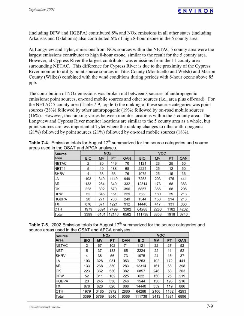
September 2004
H:\etcog3\report\sept04\sec7.doc 7-9
(including DFW and HGBPA) contributed 8% and NOx emissions in all other states (including Arkansas and Oklahoma) also contributed 6% of high 8-hour ozone in the 5 county area. At Longview and Tyler, emissions from NOx sources within the NETAC 5 county area were the largest emissions contributor to high 8-hour ozone, similar to the result for the 5 county area. However, at Cypress River the largest contributor was emissions from the 11 county area surrounding NETAC. This difference for Cypress River is due to the proximity of the Cypress River monitor to utility point source sources in Titus County (Monticello and Welsh) and Marion County (Wilkes) combined with the wind conditions during periods with 8-hour ozone above 85 ppb. The contribution of NOx emissions was broken out between 3 sources of anthropogenic emissions: point sources, on-road mobile sources and other sources (i.e., area plus off-road). For the NETAC 5 county area (Table 7-9, top left) the ranking of these source categories was point sources (28%) followed by other anthropogenic (19%) followed by on-road mobile sources (16%). However, this ranking varies between monitor locations within the 5 county area. The Longview and Cypress River monitor locations are similar to the 5 county area as a whole, but point sources are less important at Tyler where the ranking changes to other anthropogenic (21%) followed by point sources (21%) followed by on-road mobile sources (18%). Table 7-4. Emission totals for August 17th summarized for the source categories and source areas used in the OSAT and APCA analyses.
NOx VOC Source Area BIO MV PT OAN BIO MV PT OAN NETAC 2 80 149 70 1121 26 25 50 NET11 5 40 188 68 2224 25 12 50 SHRV 4 38 68 76 1075 25 15 36 LA 103 349 1149 949 7253 203 175 441 AR 133 284 349 332 12314 173 68 383 OK 223 392 670 396 6857 366 68 298 DFW 52 345 151 229 622 180 29 213 HGBPA 20 271 703 249 1544 158 214 213 TX 878 671 1221 912 14440 417 131 860 OTH 1979 3691 7499 3282 64288 2280 1182 4202 Total 3399 6161 12146 6562 111738 3853 1918 6746
Table 7-5. 2002 Emission totals for August 17th summarized for the source categories and source areas used in the OSAT and APCA analyses.
NOx VOC Source Area BIO MV PT OAN BIO MV PT OAN NETAC 2 67 102 71 1121 22 27 52 NET11 5 37 133 65 2224 22 11 52 SHRV 4 38 56 73 1075 24 15 37 LA 103 328 931 953 7253 192 172 441 AR 133 268 350 283 12314 161 68 398 OK 223 362 530 382 6857 246 68 303 DFW 52 311 102 225 622 150 25 219 HGBPA 20 245 538 246 1544 130 193 216 TX 878 628 826 888 14440 359 119 886 OTH 1979 3485 5972 2880 64288 2106 1182 4293 Total 3399 5769 9540 6066 111738 3413 1881 6896

September 2004
H:\etcog3\report\sept04\sec7.doc 7-10
Table 7-6. 2007 Emission totals for August 17th summarized for the source categories and source areas used in the OSAT and APCA analyses.
NOx VOC Source Area BIO MV PT OAN BIO MV PT OAN NETAC 2 38 116 69 1121 13 32 52 NET11 5 27 142 56 2224 14 12 53 SHRV 4 27 53 82 1075 17 7 32 LA 103 237 1082 894 7253 134 164 357 AR 133 195 274 321 12314 113 28 353 OK 223 265 648 264 6857 173 52 296 DFW 52 208 89 196 622 101 33 208 HGBPA 20 160 663 273 1544 85 247 197 TX 878 445 1082 878 14440 247 175 921 OTH 1979 2549 3866 3214 64288 1489 924 3631 Total 3399 4152 8016 6248 111738 2384 1675 6101
Table 7-7. Ratio of 2002/1999 Emission totals for August 17th summarized for the source categories and source areas used in the OSAT and APCA analyses.
NOx VOC Source Area BIO MV PT OAN BIO MV PT OAN NETAC 1.00 0.84 0.68 1.01 1.00 0.84 1.09 1.03 NET11 1.00 0.94 0.71 0.96 1.00 0.86 0.93 1.03 SHRV 1.00 1.00 0.83 0.97 1.00 0.99 1.01 1.01 LA 1.00 0.94 0.81 1.00 1.00 0.95 0.99 1.00 AR 1.00 0.94 1.00 0.85 1.00 0.93 1.00 1.04 OK 1.00 0.92 0.79 0.96 1.00 0.67 1.00 1.02 DFW 1.00 0.90 0.67 0.98 1.00 0.83 0.87 1.03 HGBPA 1.00 0.90 0.77 0.99 1.00 0.82 0.90 1.01 TX 1.00 0.94 0.68 0.97 1.00 0.86 0.91 1.03 OTH 1.00 0.94 0.80 0.88 1.00 0.92 1.00 1.02 Total 1.00 0.94 0.79 0.92 1.00 0.89 0.98 1.02
Note: The source areas are defined in Table 7-2 and the emission categories are defined in Table 7-1 Table 7-8. Ratio of 2007/1999 Emission totals for August 17th summarized for the source categories and source areas used in the OSAT and APCA analyses.
NOx VOC Source Area BIO MV PT OAN BIO MV PT OAN NETAC 1.00 0.48 0.78 0.98 1.00 0.49 1.31 1.04 NET11 1.00 0.67 0.76 0.82 1.00 0.54 1.07 1.05 SHRV 1.00 0.71 0.78 1.09 1.00 0.68 0.44 0.88 LA 1.00 0.68 0.94 0.94 1.00 0.66 0.94 0.81 AR 1.00 0.69 0.79 0.97 1.00 0.65 0.42 0.92 OK 1.00 0.68 0.97 0.67 1.00 0.47 0.77 1.00 DFW 1.00 0.60 0.59 0.86 1.00 0.56 1.14 0.98 HGBPA 1.00 0.59 0.94 1.10 1.00 0.54 1.16 0.93 TX 1.00 0.66 0.89 0.96 1.00 0.59 1.34 1.07 OTH 1.00 0.69 0.52 0.98 1.00 0.65 0.78 0.86 Total 1.00 0.67 0.66 0.95 1.00 0.62 0.87 0.90
Note: The source areas are defined in Table 7-2 and the emission categories are defined in Table 7-1

September 2004
H:\etcog3\report\sept04\sec7.doc 7-11
Table 7-9. Average ppb contributions to high 8-hour ozone for 1999 (base7).
5 NETAC Counties Longview
Source Category Source Area PT MV OAN BIO BC IC TotalNETAC 11.3 9.2 8.6 0.2 29.4 NET11 7.8 0.9 2.7 0.1 11.5 SHRV 1.0 0.5 1.1 0.1 2.6 LA 1.3 0.7 1.4 0.2 3.7 AR 0.6 0.4 0.6 0.2 1.8 OK 0.5 0.4 0.4 0.1 1.3 DFW 0.2 0.6 0.5 0.1 1.5 HGBPA 0.3 0.2 0.2 0.0 0.6 TX 1.1 0.8 1.1 0.5 3.4 OTH 2.1 1.0 1.0 0.5 4.6 N/A 32.5 0.2 32.7 Total 26.1 14.7 17.4 2.0 32.5 0.2 92.9
Tyler Cypress River
Source Category Source Area PT MV OAN BIO BC IC TotalNETAC 15.9 12.3 11.2 0.2 39.5 NET11 4.1 0.6 2.2 0.1 7.0 SHRV 1.2 0.5 1.0 0.1 2.8 LA 1.4 0.8 1.5 0.2 3.9 AR 0.6 0.4 0.6 0.2 1.7 OK 0.3 0.2 0.3 0.1 0.8 DFW 0.2 0.5 0.4 0.1 1.1 HGBPA 0.2 0.1 0.1 0.0 0.5 TX 0.8 0.6 0.8 0.4 2.5 OTH 2.3 1.0 1.0 0.5 4.8 N/A 32.3 0.1 32.4 Total 26.9 16.9 19.1 1.8 32.3 0.1 97.0
Source Category Source Area PT MV OAN BIO BC IC TotalNETAC 8.1 10.5 9.0 0.3 27.9 NET11 1.4 0.4 2.4 0.1 4.3 SHRV 1.5 0.5 1.1 0.1 3.2 LA 2.0 0.9 2.1 0.5 5.5 AR 1.4 1.0 1.4 0.4 4.2 OK 0.2 0.2 0.2 0.0 0.6 DFW 0.0 0.0 0.0 0.0 0.1 HGBPA 0.3 0.1 0.1 0.0 0.5 TX 0.2 0.3 0.6 0.1 1.3 OTH 2.6 1.2 1.4 0.8 6.0 N/A 32.4 0.0 32.4 Total 17.7 15.1 18.4 2.3 32.4 0.0 85.8
Source Category Source Area PT MV OAN BIO BC IC TotalNETAC 4.6 2.9 3.4 0.1 11.1 NET11 21.8 1.9 7.1 0.2 31.0 SHRV 1.0 0.7 1.4 0.1 3.2 LA 1.1 0.7 1.4 0.2 3.4 AR 1.1 0.6 1.0 0.3 3.0 OK 0.1 0.1 0.1 0.0 0.2 DFW 0.0 0.0 0.0 0.0 0.0 HGBPA 0.1 0.0 0.0 0.0 0.1 TX 1.2 1.7 2.7 0.3 5.9 OTH 1.9 0.8 0.8 0.4 3.8 N/A 33.3 0.1 33.4 Total 32.8 9.4 17.8 1.6 33.3 0.1 95.0

September 2004
H:\etcog3\report\sept04\sec7.doc 7-12
OZONE CONTRIBUTIONS FOR 2002 AND 2007 The analysis of the 2002 and 2007 base case results (Tables 7-10 and 7-11) was designed to be consistent with the 1999 analysis so that source contributions can be compared directly between years. In order to obtain a direct comparison, the ozone contributions must be averaged over the same set of grid cells and hours in all years. Therefore, the 2002/2007 source contributions were averaged for the grid cells and hours when the 1999 ozone levels were 85 ppb or higher. Table 7-10. Average ppb contributions1 to high 8-hour ozone for 2002 (02base3).
5 NETAC Counties
Source Category Source Area PT MV OAN BIO BC IC TotalNETAC 8.8 8.3 9.3 0.2 26.7 NET11 6.0 0.9 2.7 0.2 9.8 SHRV 0.9 0.5 1.0 0.1 2.5 LA 1.2 0.7 1.5 0.2 3.5 AR 0.6 0.4 0.5 0.2 1.7 OK 0.4 0.4 0.4 0.1 1.2 DFW 0.2 0.6 0.5 0.1 1.4 HGBPA 0.2 0.1 0.2 0.0 0.5 TX 0.6 0.9 1.0 0.5 3.0 OTH 1.8 1.0 0.9 0.5 4.2 N/A 32.7 0.2 32.8 Total 20.6 13.8 18.1 2.1 32.7 0.2 87.3
Tyler Source Category Source
Area PT MV OAN BIO BC IC TotalNETAC 6.9 9.5 9.3 0.3 26.1 NET11 1.2 0.4 2.4 0.1 4.1 SHRV 1.4 0.5 1.1 0.1 3.1 LA 1.9 0.9 2.1 0.5 5.3 AR 1.4 0.9 1.2 0.5 4.0 OK 0.2 0.2 0.2 0.0 0.5 DFW 0.0 0.0 0.0 0.0 0.1 HGBPA 0.3 0.1 0.1 0.0 0.4 TX 0.2 0.3 0.6 0.1 1.2 OTH 2.0 1.2 1.3 0.8 5.4 N/A 32.3 0.0 32.3 Total 15.4 14.0 18.3 2.4 32.3 0.0 82.4
1. Contributions are averaged over all grid cells and hours that had 8-hour ozone of 85 ppb or higher in the 1999 base case.
Longview Source Category Source
Area PT MV OAN BIO BC IC TotalNETAC 12.1 11.4 12.4 0.2 36.1 NET11 3.4 0.6 2.3 0.1 6.4 SHRV 1.2 0.5 1.0 0.1 2.7 LA 1.3 0.7 1.5 0.3 3.8 AR 0.5 0.4 0.6 0.2 1.7 OK 0.3 0.2 0.3 0.1 0.8 DFW 0.1 0.4 0.4 0.1 1.0 HGBPA 0.2 0.1 0.1 0.0 0.5 TX 0.5 0.6 0.7 0.4 2.2 OTH 1.9 1.0 1.0 0.5 4.4 N/A 32.7 0.1 32.8 Total 21.4 16.0 20.3 1.9 32.7 0.1 92.4
Cypress River Source Category Source
Area PT MV OAN BIO BC IC TotalNETAC 3.4 2.7 3.7 0.1 9.9 NET11 13.2 2.0 7.0 0.3 22.5 SHRV 0.9 0.7 1.4 0.1 3.0 LA 1.0 0.6 1.4 0.2 3.3 AR 1.1 0.6 0.8 0.3 2.8 OK 0.1 0.1 0.1 0.0 0.2 DFW 0.0 0.0 0.0 0.0 0.0 HGBPA 0.0 0.0 0.0 0.0 0.1 TX 1.2 1.8 2.6 0.3 5.9 OTH 1.5 0.8 0.7 0.4 3.5 N/A 33.0 0.1 33.0 Total 22.5 9.3 17.7 1.7 33.0 0.1 84.2

September 2004
H:\etcog3\report\sept04\sec7.doc 7-13
Table 7-11. Average ppb contributions1 to high 8-hour ozone for 2007 (07base5).
5 NETAC Counties Source Category Source
Area PT MV OAN BIO BC IC TotalNETAC 10.5 5.2 9.6 0.3 25.6 NET11 6.3 0.7 2.3 0.2 9.5 SHRV 0.9 0.4 1.2 0.1 2.5 LA 1.5 0.5 1.3 0.2 3.5 AR 0.4 0.3 0.6 0.2 1.5 OK 0.4 0.3 0.2 0.1 1.0 DFW 0.2 0.4 0.5 0.1 1.2 HGBPA 0.3 0.1 0.2 0.0 0.6 TX 1.0 0.6 0.9 0.5 3.0 OTH 1.0 0.7 1.3 0.5 3.6 N/A 32.6 0.2 32.8 Total 22.5 9.2 18.1 2.2 32.6 0.2 84.7
Tyler Source Category Source
Area PT MV OAN BIO BC IC TotalNETAC 8.2 6.6 9.5 0.3 24.6 NET11 1.5 0.3 2.3 0.1 4.2 SHRV 1.2 0.4 1.3 0.1 2.9 LA 2.5 0.6 2.1 0.5 5.7 AR 1.1 0.7 1.3 0.5 3.6 OK 0.2 0.1 0.1 0.0 0.5 DFW 0.0 0.0 0.0 0.0 0.1 HGBPA 0.3 0.1 0.1 0.0 0.5 TX 0.3 0.2 0.5 0.1 1.2 OTH 1.1 0.9 1.7 0.9 4.6 N/A 32.1 0.0 32.1 Total 16.5 10.0 18.8 2.5 32.1 0.0 79.9
1. Contributions are averaged over all grid cells and hours that had 8-hour ozone of 85 ppb or higher in the 1999 base case.
Longview Source Category Source
Area PT MV OAN BIO BC IC TotalNETAC 15.4 7.0 13.2 0.2 35.8 NET11 3.6 0.5 2.1 0.1 6.2 SHRV 1.0 0.4 1.2 0.1 2.6 LA 1.6 0.5 1.4 0.3 3.8 AR 0.5 0.3 0.6 0.2 1.6 OK 0.3 0.2 0.2 0.1 0.7 DFW 0.1 0.3 0.4 0.1 0.9 HGBPA 0.3 0.1 0.2 0.0 0.5 TX 0.8 0.5 0.7 0.4 2.3 OTH 1.1 0.7 1.4 0.6 3.8 N/A 32.6 0.1 32.8 Total 24.6 10.5 21.1 2.1 32.6 0.1 91.0
Cypress River Source Category Source
Area PT MV OAN BIO BC IC TotalNETAC 4.0 1.7 3.7 0.1 9.5 NET11 14.6 1.5 4.5 0.3 20.9 SHRV 0.8 0.5 1.6 0.1 3.0 LA 1.3 0.5 1.2 0.2 3.3 AR 0.6 0.5 0.9 0.3 2.3 OK 0.1 0.0 0.0 0.0 0.2 DFW 0.0 0.0 0.0 0.0 0.0 HGBPA 0.1 0.0 0.0 0.0 0.1 TX 1.0 1.4 2.3 0.3 4.9 OTH 0.8 0.6 1.1 0.4 2.9 N/A 33.0 0.1 33.1 Total 23.3 6.7 15.4 1.8 33.0 0.1 80.3

September 2004
H:\etcog3\report\sept04\sec7.doc 7-14
EMISSIONS CHANGES BETWEEN 1999, 2002 AND 2007 One of the outputs from a CAMx OSAT or APCA analysis is a summary of the emissions for each source grouping. Tables 7-4 to 7-6 show the emissions summaries for 1999, 2002 and 2007. Ratios of 2002/1999 emissions are shown in Table 7-7 and ratios of 2007/1999 emissions are shown in Table 7-8. These emission summaries are useful for comparison with the APCA source apportionment results but they are less accurate than the detailed emissions summaries reported in Section 3 for the following reasons. The emission summaries are all for the August 17th episode, other days may be different. These emissions summaries are prepared from the gridded emissions, and so areas are defined geographically to the nearest grid cell boundary, which means that emission totals may not exactly match those reported in Section 3. Finally, it is impossible to exactly calculate tons of VOCs from model ready inventories (because the model ready emissions are in moles, not tons) so the VOC emission totals will differ from those reported in Section 3. Emissions Changes From 1999 to 2007 On-road mobile source emissions decreased over all by 33% for NOx and 38% for VOC between 1999 and 2007. These reductions result from improvements in vehicle technology and fuels in response to EPA rules for light-duty and heavy-duty vehicles (plus local measures in nonattainment areas). The vehicle technology and fuel improvements are partially offset by growth in VMT. Larger percentage reductions occurred in the DFW and HGBPA nonattainment areas than most of Texas due to local SIP measures. The largest percentage decrease in on-road mobile source NOx emissions was in the NETAC 5 county area due to a large decrease in NOx from truck traffic on Interstate-20. NOx emissions from heavy-duty trucks are projected to decrease significantly between 1999 and 2007 due to EPA regulations, and truck emissions make a relatively high contribution to on-road NOx in the NETAC area because I-20 runs across Smith, Gregg and Harrison Counties (see Figure 1-3). The Texas on-road mobile emissions were estimated by TTI for the TCEQ. All the on-road mobile source emissions are based on MOBILE6. Point source emissions decreased over-all by 34% for NOx and 13% for VOC between 1999 and 2007. The largest percentage NOx reductions occurred in the states outside TX, LA, AR and OK and are due primarily to the effects of EPA’s “NOx SIP call.” NOx emissions in the NETAC 5 county area decreased by 22% (for August 17th) and NOx emissions in the surrounding 11 counties decreased by 24%. The decreases in Northeast Texas point source NOx result from NETAC measures included in the Northeast Texas 1-hour ozone SIP revision and TCEQ rules for Eastern Texas. The percentage decrease in point source NOx in Northeast Texas was larger than in the rest of Texas except for the DFW nonattainment area where deep point source NOx reductions are included in the SIP. The point source NOx reductions for the HGBPA nonattainment area are only 6% in these inventories but are expected to become greater as more Houston SIP rules are implemented. The percentage decrease in point source NOx in Northeast Texas also was larger than for LA and OK. The percent changes in point source VOC were highly variable and are not discussed. The point source emission changes for Northeast Texas were estimated by NETAC, for the remainder of Texas by TCEQ, and for all other areas by EPA. Other anthropogenic (i.e., area plus off-road) emissions decreased over-all by 5% for NOx and 10% for VOC between 1999 and 2007. These over-all percentage reductions are smaller than for

September 2004
H:\etcog3\report\sept04\sec7.doc 7-15
on-road mobile sources and point sources. In the NETAC 5 county area, other anthropogenic NOx emissions decreased by 2% and other anthropogenic VOC increased by 4% because the effects of growth offset the effects of controls. All the off-road source emissions were based on the EPA’s NONROAD2002 model. There were no changes in the biogenic emissions between 1999 and 2007. Emissions Changes From 1999 to 2002 The changes in NETAC area NOx emissions for 2002 and 20007 relative to 1999 are as follows. On-road mobile NOx decreased by 16% in 2002 and 52% in 2007. The 2007 decrease is greater because EPA’s heavy-duty vehicle NOx reductions phase-in more strongly after 2002. Point source NOx decreased by 32% in 2002 and 22% in 2007. The smaller decrease for 2002 than 2007 results from the way the emissions were estimated. NETAC area EGU emissions were based on July-September average actual emissions for 2002 whereas for 2007 they were episodic values assuming high heat input rates and permit-limit emission factors. Thus, the higher NETAC point-source emissions for 2007 than 2002 do not indicate an expected real-world increase in emissions, and this assumption will have a conservative effect in the 8-hour ozone attainment demonstration. Other anthropogenic NOx increased by 1% in 2002 and decreased by 2% in 2007 The changes in over-all NOx emissions for 2002 and 20007 relative to 1999 are as follows. On-road mobile NOx decreased 6% in 2002 and 33% in 2007. The 2007 decrease is greater because EPA’s heavy-duty vehicle NOx reductions phase-in more strongly after 2002. Point-source NOx decreased 21% in 2002 and 34% in 2007. The 2007 decrease is greater primarily due to the phase-in of EPA’s “NOx SIP call.” Other anthropogenic NOx decreased by 8% in 2002 and 5% in 2007. CHANGES IN OZONE BETWEEN 1999 AND 2007 The changes in ozone contributions between 1999, 2002 and 2007 are shown in Tables 7-10 and 7-11 and are illustrated using bar charts in Figure 7-4. The discussion of these results is limited to the changes from 1999 to 2007 to focus on the attainment demonstration year. NETAC 5 County Area For the NETAC 5 county area the total reduction in high 8-hour ozone was –8.1 ppb (Table 7-13, top left). There were reduced contributions from on-road mobile source NOx (–5.4 ppb) and point source NOx (–3.86 ppb) but a small increase in the contribution of other anthropogenic NOx (0.6 ppb). Looking at the geographic contributions to ozone reductions, the largest reductions were from the NETAC area (–3.8 ppb) and the 11 counties surrounding NETAC (–2.0 ppb) with smaller reductions from other areas. These combined reductions from the NETAC area and surrounding 11 counties accounted for 72% of the total reduction of –8.1 ppb.

September 2004
H:\etcog3\report\sept04\sec7.doc 7-16
Looking in detail at the ozone reductions from emissions sources in Northeast Texas, the largest reductions were from on-road mobile sources (–4.0 ppb) and point sources (–0.8 ppb), which is consistent with the NOx emissions reductions for these categories shown in Table 7-8. The ozone contribution from other anthropogenic NOx emissions increased by 1.0 ppb even though the emissions decreased slightly (2%, Table 7-8). This is a consequence of the non-linear relationship between ozone and NOx emissions whereby reducing NOx from point and on-road mobile source emissions causes more efficient ozone formation from the remaining other anthropogenic NOx. Longview The total reduction in high 8-hour ozone at Longview (–6.1 ppb, Table 7-13, top right) was smaller than for the NETAC 5 county area. This is partly because the decreases in contributions of local on-road mobile source NOx emissions (–5.2 ppb) and local point source NOx emissions (–0.6 ppb) were offset by increase in the contributions from local other anthropogenic NOx emissions (2.0 ppb). Tyler The total reduction in high 8-hour ozone was –5.9 ppb at Tyler (Table 7-13, bottom left), which was smaller than the total reductions for the NETAC 5 county area and for Longview. The reduction in ozone from Northeast Texas emissions was –3.2 ppb, which was entirely due to reductions from on-road mobile sources of –3.9 ppb. Cypress River The total reduction in high 8-hour ozone was –14.7 ppb at Cypress River (Table 7-13, bottom right), which was much larger than for the other receptor areas. This large reduction was due to a large decrease of –10.1 ppb in the contribution of point source NOx in the 11 counties surrounding NETAC. This is related to the proximity of the Cypress River monitor to utility point sources in Titus County (Monticello and Welsh) and Marion County (Wilkes). The emissions reductions at these sources (from Section 3) are Monticello (76%), Welsh (57%) and Wilkes (50%) averaged over all episode days.

September 2004
H:\etcog3\report\sept04\sec7.doc 7-17
Table 7-12. Change in average contributions to high 8-hour ozone between 1999 (base7) and 2002 (02base3).
5 NETAC Counties
Source Category Source Area PT MV OAN BIO BC IC TotalNETAC -2.5 -0.9 0.7 0.0 -2.7 NET11 -1.8 0.0 0.1 0.0 -1.7 SHRV -0.1 0.0 0.0 0.0 -0.1 LA -0.1 0.0 0.0 0.0 -0.1 AR 0.0 0.0 -0.1 0.0 -0.1 OK -0.1 0.0 0.0 0.0 -0.1 DFW -0.1 0.0 0.0 0.0 -0.1 HGBPA 0.0 0.0 0.0 0.0 0.0 TX -0.4 0.0 0.0 0.0 -0.4 OTH -0.3 0.0 -0.1 0.0 -0.4 N/A 0.1 0.0 0.1 Total -5.5 -0.9 0.6 0.1 0.1 0.0 -5.5
Tyler Source Category Source
Area PT MV OAN BIO BC IC TotalNETAC -1.2 -1.0 0.3 0.0 -1.8 NET11 -0.1 0.0 0.0 0.0 -0.2 SHRV -0.1 0.0 0.0 0.0 -0.1 LA -0.2 -0.1 0.0 0.0 -0.2 AR 0.0 0.0 -0.2 0.0 -0.2 OK 0.0 0.0 0.0 0.0 0.0 DFW 0.0 0.0 0.0 0.0 0.0 HGBPA 0.0 0.0 0.0 0.0 0.0 TX 0.0 0.0 0.0 0.0 -0.1 OTH -0.6 0.0 -0.1 0.0 -0.6 N/A -0.1 0.0 -0.1 Total -2.3 -1.1 -0.1 0.1 -0.1 0.0 -3.4
Longview Source Category Source
Area PT MV OAN BIO BC IC TotalNETAC -3.9 -0.9 1.3 0.0 -3.5 NET11 -0.7 0.0 0.1 0.0 -0.6 SHRV -0.1 0.0 0.0 0.0 0.0 LA -0.1 0.0 0.0 0.0 -0.1 AR 0.0 0.0 -0.1 0.0 -0.1 OK -0.1 0.0 0.0 0.0 0.0 DFW 0.0 0.0 0.0 0.0 0.0 HGBPA 0.0 0.0 0.0 0.0 0.0 TX -0.3 0.0 0.0 0.0 -0.3 OTH -0.4 0.0 0.0 0.0 -0.4 N/A 0.4 0.0 0.4 Total -5.5 -0.9 1.3 0.1 0.4 0.0 -4.7
Cypress River Source Category Source
Area PT MV OAN BIO BC IC TotalNETAC -1.2 -0.3 0.3 0.0 -1.1 NET11 -8.6 0.1 -0.1 0.0 -8.6 SHRV -0.2 0.0 0.0 0.0 -0.2 LA -0.1 0.0 0.0 0.0 -0.1 AR 0.0 0.0 -0.2 0.0 -0.2 OK 0.0 0.0 0.0 0.0 0.0 DFW 0.0 0.0 0.0 0.0 0.0 HGBPA 0.0 0.0 0.0 0.0 0.0 TX 0.0 0.1 -0.1 0.0 0.0 OTH -0.3 0.0 -0.1 0.0 -0.4 N/A -0.3 0.0 -0.3 Total -10.4 -0.1 -0.1 0.1 -0.3 0.0 -10.8
Note: Contributions are averaged over all grid cells and hours that had 8-hour ozone of 85 ppb or higher in the 1999 base case. Negative values mean a smaller contribution in 2002 than 1999.

September 2004
H:\etcog3\report\sept04\sec7.doc 7-18
Table 7-13. Change in average contributions to high 8-hour ozone between 1999 (base7) and 2007 (07base5).
5 NETAC Counties
Source Category Source Area PT MV OAN BIO BC IC TotalNETAC -0.8 -4.0 1.0 0.0 -3.8 NET11 -1.5 -0.2 -0.3 0.0 -2.0 SHRV -0.1 -0.1 0.2 0.0 -0.1 LA 0.2 -0.2 -0.2 0.0 -0.2 AR -0.2 -0.1 0.0 0.0 -0.3 OK 0.0 -0.1 -0.2 0.0 -0.3 DFW -0.1 -0.2 0.0 0.0 -0.2 HGBPA 0.0 -0.1 0.0 0.0 0.0 TX -0.1 -0.2 -0.1 0.0 -0.4 OTH -1.1 -0.3 0.3 0.1 -1.0 N/A 0.1 0.0 0.1 Total -3.6 -5.4 0.6 0.2 0.1 0.0 -8.1
Tyler Source Category Source
Area PT MV OAN BIO BC IC TotalNETAC 0.1 -3.9 0.5 0.0 -3.2 NET11 0.1 -0.1 -0.1 0.0 -0.1 SHRV -0.3 -0.1 0.1 0.0 -0.3 LA 0.5 -0.3 -0.1 0.0 0.2 AR -0.3 -0.3 0.0 0.1 -0.6 OK 0.0 -0.1 -0.1 0.0 -0.1 DFW 0.0 0.0 0.0 0.0 0.0 HGBPA 0.0 0.0 0.0 0.0 0.0 TX 0.1 -0.1 -0.1 0.0 -0.1 OTH -1.5 -0.3 0.3 0.1 -1.4 N/A -0.3 0.0 -0.3 Total -1.2 -5.2 0.5 0.2 -0.3 0.0 -5.9
Longview Source Category Source
Area PT MV OAN BIO BC IC TotalNETAC -0.6 -5.2 2.0 0.0 -3.7 NET11 -0.5 -0.1 -0.1 0.0 -0.8 SHRV -0.2 -0.1 0.2 0.0 -0.1 LA 0.2 -0.2 -0.2 0.0 -0.1 AR -0.1 -0.1 0.0 0.0 -0.1 OK 0.0 -0.1 -0.1 0.0 -0.2 DFW 0.0 -0.1 0.0 0.0 -0.2 HGBPA 0.0 0.0 0.0 0.0 0.0 TX 0.0 -0.2 -0.1 0.0 -0.2 OTH -1.2 -0.3 0.3 0.1 -1.0 N/A 0.4 0.0 0.4 Total -2.3 -6.4 2.1 0.3 0.3 0.0 -6.1
Cypress River Source Category Source
Area PT MV OAN BIO BC IC TotalNETAC -0.7 -1.2 0.4 0.0 -1.5 NET11 -7.2 -0.4 -2.5 0.0 -10.1 SHRV -0.2 -0.2 0.2 0.0 -0.2 LA 0.3 -0.2 -0.2 0.0 -0.1 AR -0.5 -0.2 -0.1 0.0 -0.7 OK 0.0 0.0 -0.1 0.0 0.0 DFW 0.0 0.0 0.0 0.0 0.0 HGBPA 0.0 0.0 0.0 0.0 0.0 TX -0.2 -0.3 -0.5 0.0 -0.9 OTH -1.1 -0.2 0.3 0.1 -0.9 N/A -0.2 0.0 -0.2 Total -9.6 -2.7 -2.4 0.2 -0.2 0.0 -14.7
Note: Contributions are averaged over all grid cells and hours that had 8-hour ozone of 85 ppb or higher in the 1999 base case. Negative values mean a smaller contribution in 2007 than 1999.

September 2004
H:\etcog3\report\sept04\sec7.doc 7-19
Source Category Source Area
Figure 7-4. Comparison of 1999, 2002 and 2007 average ppb contributions to 8-hour ozone of 85 ppb and higher. SUMMARY AND CONCLUSIONS The ozone source apportionment analysis provides insight into the sensitivity of modeled ozone levels to emissions, boundary conditions and initial conditions in 1999 and 2007. This information leads to the following conclusions about the model configuration, the sources that contribute to high ozone and the effectiveness of emissions reductions.

September 2004
H:\etcog3\report\sept04\sec7.doc 7-20
Model Configuration • Initial conditions were unimportant. This shows that the model spin-up period was
sufficient. • Boundary conditions contributed about 33 ppb to 8-hour ozone levels above 85 ppb in
Northeast Texas in 1999, 2002 and 2007. Since the boundary condition for ozone was set to 40 ppb, about 25% of the boundary ozone was destroyed by chemistry and deposition before reaching Northeast Texas. This level of influence from the boundary conditions is appropriate and shows that the modeling is not overly influenced by boundary condition assumptions. The boundary influence is constant across years because the boundary conditions were held constant.
• Emissions in states outside of Texas, Louisiana, Arkansas and Oklahoma contributed about 4
ppb to 8-hour ozone above 85 ppb in Northeast Texas. This contribution is about 5% of the high 8-hour ozone which shows that:
• High 8-hour ozone levels in Northeast Texas during this episode were primarily due to
emissions from within a “1-state” distance upwind. • The 12-km modeling domain is large enough to capture most of the important upwind
emissions influence from Texas, Louisiana, Arkansas and Oklahoma.
• Emissions from Northeast Texas (NETAC 5 counties plus the surrounding 11 counties) and Shreveport contributed about 44 ppb of 8-hour ozone above 85 ppb in Northeast Texas in 1999. This shows that the 4-km modeling domain is large enough to capture more than 50% of the important emissions influences.
Ozone Sensitivity to Emissions • The majority (more than 62%) of high 8-hour ozone in the NETAC 5 county area in 1999
was attributed to anthropogenic emissions sources. This means that 8-hour ozone can be reduced by controlling the appropriate emissions sources.
• Controlling NOx emissions is the only effective strategy for reducing high 8-hour ozone.
Ozone formation is predominantly NOx sensitive on moderately high 8-hour ozone days, but on the highest ozone days (i.e., with the most stagnant meteorology) ozone is sensitive to both NOx and VOCs. However, because the VOCs are dominated by biogenic emissions, NOx control is the most effective strategy on all days. Emissions of highly reactive VOCs close to a monitor may be an exceptional case.
Source Contributions in 1999 • The largest emissions contributions to high 8-hour ozone in the NETAC 5 county area come
from nearby NOx emissions. Nearby means primarily emissions from within the 5 county NETAC area, followed by emissions in surrounding counties, followed by emissions from
September 2004
H:\etcog3\report\sept04\sec7.doc 7-21
Louisiana. The contribution from Louisiana is split about evenly between the 4 parish Shreveport area and the rest of the state.
• The relative importance of different source categories of NOx emission varies by location
within the NETAC area. For the 5 county region as a whole and for Longview and Cypress River, point sources are the largest contributor followed by area/off-road sources followed by motor vehicles. At Tyler, area/off-road sources are the largest contributor followed by point sources followed by motor vehicles.
• The contribution to high 8-hour ozone in the NETAC 5 county area from emissions in the 5
Counties was 29.4 ppb and from the surrounding 11 Counties was 11.5 ppb. • The contribution to high 8-hour ozone in the NETAC 5 county area from Dallas/Fort Worth
was 1.5 ppb, from Houston/Galveston/Beaumont/Port Arthur was 0.6 ppb and from the rest of Texas was 3.4 ppb.
• The contribution to high 8-hour ozone in the NETAC 5 county area from Shreveport was 2.6
ppb, the rest of Louisiana was 3.7 ppb, Arkansas was 1.8 ppb and Oklahoma was 1.3 ppb. • The contribution to high 8-hour ozone in the NETAC 5 county area from states outside
Texas, Louisiana, Arkansas and Oklahoma was 4.4 ppb. Emissions Changes between 1999 and 2007 Emissions changes were analyzed for the August 17th episode day and may be different for other episode days. • NOx emissions in the NETAC 5 county area decreased by –52% for on-road mobile sources
and –22% for point sources and –2% for other anthropogenic sources (area plus off-road). Ozone Changes between 1999 and 2007 • High 8-hour ozone in the NETAC 5 county area was reduced by –8.1 ppb between 1999 and
2007. There were reduced contributions from point source NOx (–3.6 ppb) and on-road mobile source NOx (–5.4 ppb) but a small increase in the contribution of other anthropogenic NOx (0.6 ppb).
• The 0.6 ppb increase in the ozone contribution from other anthropogenic NOx emissions is
explained by more efficient ozone formation from NOx emissions as total NOx levels are reduced. This is an example of the non-linear relationship between ozone and NOx emissions.
• The non-linear relationship between ozone and NOx is most pronounced in areas with
relatively high NOx emissions, such as the Longview monitor area. The consequence is that high 8-hour ozone levels at Longview are resistant to NOx reductions, even though NOx
September 2004
H:\etcog3\report\sept04\sec7.doc 7-22
reduction is the most effective strategy. In other words, an X% reduction in local NOx emissions will lead to less than an X% reduction in ozone at Longview.
• The contribution to high 8-hour ozone in the NETAC 5 county area from the rest of Texas
(i.e., outside the 16 counties in Northeast Texas) decreased by –0.6 ppb. • There were small changes between 1999 and 2007 in the contributions to high 8-hour ozone
in the NETAC 5 county area from Shreveport (–0.1 ppb), the rest of Louisiana (–0.2 ppb), Arkansas (–0.3 ppb) and Oklahoma (–0.3 ppb).
• Although the contribution of emissions from states outside Texas, Louisiana, Arkansas and
Oklahoma was small (4.6ppb in 1999), this contribution was reduced by –1.0 ppb in 2007 showing benefits from emissions reductions strategies for the Eastern U.S. such as EPA’s “NOx SIP call” and cleaner on-road vehicles and fuels.

September 2004
H:\etcog3\report\sept04\Refs.doc R-1
REFERENCES Coulter-Burke, S., D. Calkins and G. Yarwood. 2002. “Analysis of Emission Reduction Control
Measures for Attaining the 8-Hour Ozone NAAQS in the Tyler/Longview/ Marshall Near Nonattainment Area.” Prepared for the East Texas Council of Governments by ENVIRON International Corporation, 101 Rowland Way, Novato, CA 94945. August.
Dudhia, J., 1993. "A Non-hydrostatic Version of the Penn State/NCAR Mesoscale Model:
Validation Tests and Simulation of an Atlantic Cyclone and Cold Front", Mon. Wea. Rev., Vol. 121. pp. 1493-1513.
Dunker, A.M., G. Yarwood, J. Ortmann, and G.M. Wilson. 2002a. The decoupled direct
method for sensitivity analysis in a three-dimensional air quality model – Implementation, accuracy and efficiency. Environ. Sci. and Tech., 36, 2965-2976.
Dunker, A.M., G. Yarwood, J. Ortmann, and G.M. Wilson. 2002b. Comparison of source
apportionment and source sensitivity of ozone in a three-dimensional air quality model. Environ. Sci. and Tech., 36, 2953-2964.
Emery, C., E. Tai and Y. Jia, 2003. “Revised Meteorological Modeling of the August 13-22,
1999 East Texas Ozone Episode.” Prepared for the East Texas Council of Governments by ENVIRON International Corporation, 101 Rowland Way, Novato, CA 94945. January 23.
Emery, C. and E. Tai, 2002. “Meteorological Modeling and Performance Evaluation of the
August 13-22, 1999 Ozone Episode.” Prepared for the East Texas Council of Governments by ENVIRON International Corporation, 101 Rowland Way, Novato, CA 94945. August.
ENVIRON. 2004. “User’s Guide to the Comprehensive Air Quality Model with Extensions,
Version 4.00” available from ENVIRON International Corporation, 101 Rowland Way, Novato, CA 94945 and at http//www.camx.com. January 2004.
ENVIRON. 2003. “Modeling Protocol: Ozone Modeling for the Northeast Texas Early Action
Compact.” Report prepared for the East Texas Council of Governments by ENVIRON International Corporation, 101 Rowland Way, Novato, CA 94945. August 2003.
ENVIRON. 2002. “User’s Guide to the Comprehensive Air Quality model with extentsions,
version 3.10” available from www.camx.com. April. ENVIRON. 2000. “Conceptual Model for 8-Hour Ozone in East Texas and Episode Selection
for New Photochemical Modeling.” Prepared for the East Texas Council of Governments by ENVIRON International Corporation, 101 Rowland Way, Novato, CA 94945. 12 September.
ENVIRON. 1999. “A Biogenic Emission Inventory for the Tyler/Longview/Marshall Area
Based on Local Data.” Prepared for the East Texas Council of Governments by ENVIRON International Corporation, 101 Rowland Way, Novato, CA 94945. March.

September 2004
H:\etcog3\report\sept04\Refs.doc R-2
EPA. 1999. “Draft Guidance on the Use of Models and Other Analyses in Attainment Demonstrations for the 8-Hour Ozone NAAQS”. EPA-454/R-99-004. EPA Office of Air Quality Planning and Standards, Research Triangle Park, NC 27711. May.
Goldan, P.D., W.C. Kuster, and F.C. Fehsenfeld. 1995. “Hydrocarbon Measurements in the
Southeastern United States: The Rural Oxidants in the Southern Environment (ROSE) Program 1990.” J. Geophysical Research, vol. 100, No.D12, pp. 25945-25963.
Guenther, A., C. Wiedinmyer, B. Baugh, S. Shepard, U. Ganesh, and G. Yarwood. 2002.
“Biogenic VOC Emission Estimates for the TexAQS 2000 Emission Inventory: Estimating Emissions During Periods of Drought and Prolonged High Temperatures and Developing GloBEIS3”. Prepared for Texas Natural Resource Conservation Commission, Austin, TX. April.
Madronich, S. 2002. The Tropospheric visible Ultra-violet (TUV) model web page.
http://www.acd.ucar.edu/TUV/. Madronich, S. 1993. “UV radiation in the natural and perturbed atmosphere”, in Environmental
Effects of UV (Ultraviolet) Radiation (M. Tevini, ed.), Lewis Publisher, Boca Raton, pp. 17-69.
Pollution Solutions. 2002. Tyler/Longview/Marshall Flexible Attainment Region Emission
Inventory. Ozone Precursors, VOC and NOx 1999 Emissions. Prepared for the East Texas Council of Governments by Pollution Solutions, 3000 Taku Road, Cedar Park, TX 78613. May.
Stoeckenius T., and G. Yarwood. 2004. “Conceptual Model of Ozone Formation in the
Tyler/Longview/Marshall Near Nonattainment Area.” Report prepared for the East Texas Council of Governments by ENVIRON International Corporation, 101 Rowland Way, Novato, CA 94945. January 2004.
TNRCC. 2002. "Revisions to the State Implementation Plan (SIP) for the Control of Ozone Air
Pollution Northeast Texas Region Ozone SIP Revision." Texas Natural Resource Conservation Commission P.O. Box 13087 Austin, Texas 78711-3087. Rule Log Number 2001-026-SIP-AI March 13, 2002.
Watkins, B.A., D.D. Parrish, S. Buhr, R.B. Norton, M. Trainer, J.E. Yee, and F.C. Fehsenfeld.
1995. “Factors Influencing the Concentration of Gas Phase Hydrogen Peroxide During the Summer at Kinterbish, Alabama”. J. Geophysical Research, vol. 100, No. 311, pp. 22841-22851.
Yarwood, G. M. Jimenez, C. Emery, E. Tai. C. Tana and S. Lau. 2003. “Modeling an August
1999 Ozone Episode in Northeast Texas.” Final Report to the East Texas Council of Governments, Kilgore, TX. May.
Yarwood, G., G. Wilson, S. Shepard, and A. Guenther. 2002. User's Guide to the Global
Biosphere Emissions and Interactions System - Version 3.0. Available from http://www.globeis.com.

September 2004
H:\etcog3\report\sept04\Refs.doc R-3
Yarwood, G. G. Mansell, G. McGauhey, and W. Vizuete. 2001. “Biogenic Emission Inventories For Regional Modeling of 1999 Ozone Episodes In Texas”. Final Report to the Texas Natural Resource Conservation Commission, Austin, TX. April.

Appendix A
Spatial Maps of Estimated and Observed Daily Maximum 8-Hour Ozone (ppb)
in the 4-km Grid For the August 15–22, 1999 Episode:
1999 Base Case 7
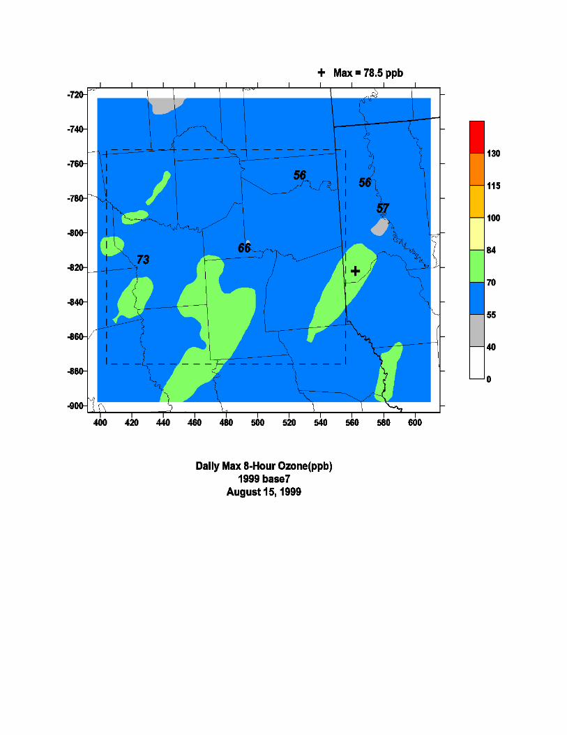


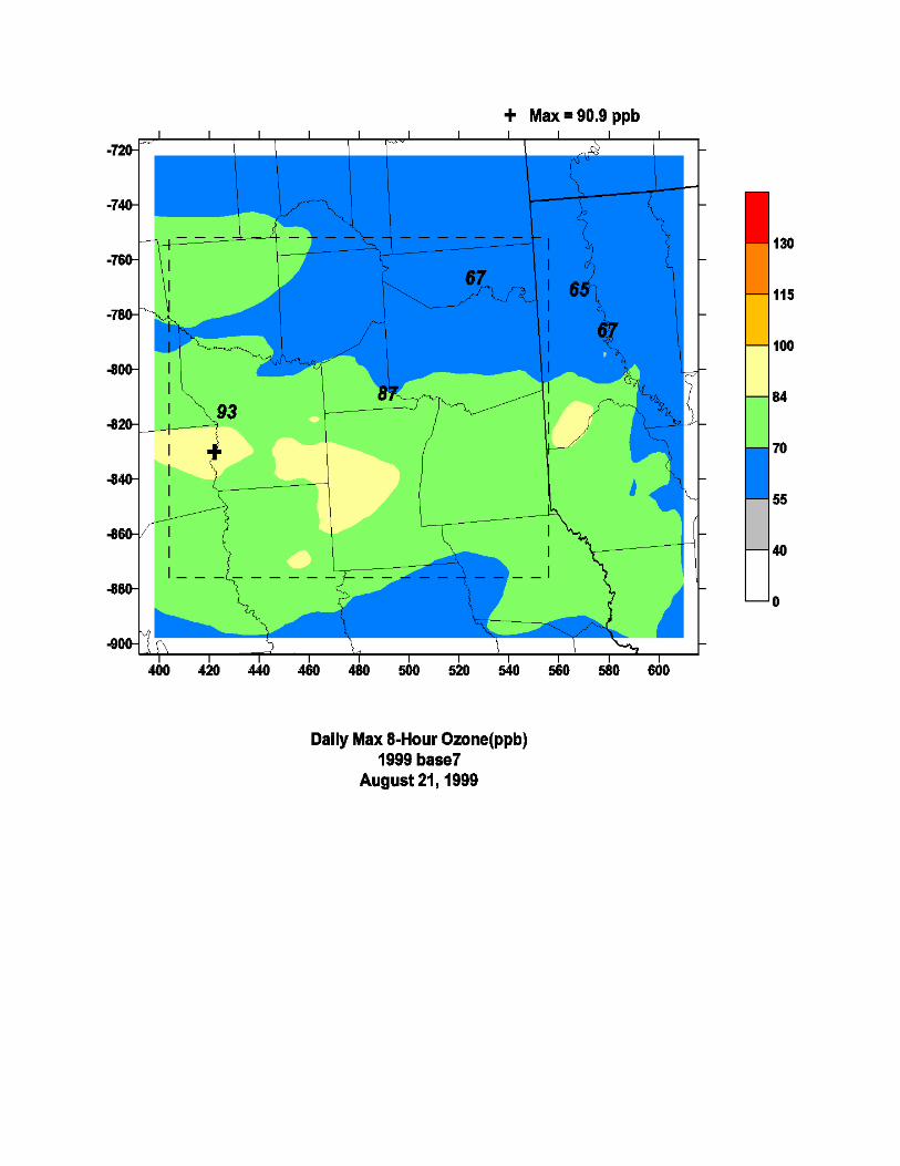


Appendix B
Spatial Maps of Estimated Daily Maximum 8-Hour Ozone (ppb)
in the 12-km Grid For the August 15–22, 1999 Episode:
1999 Base Case 7


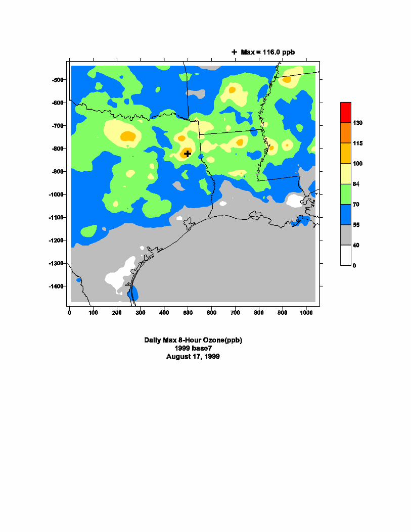


Appendix C
Spatial Maps of Estimated Daily Maximum 8-Hour Ozone (ppb)
in the 4-km Grid for the August 15–22, 1999 Episode:
2002 Base Case 3


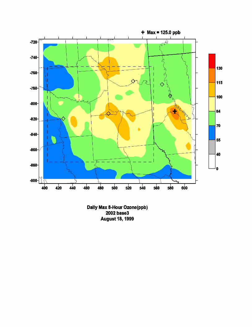


Appendix D
Spatial Maps of Estimated Daily Maximum 8-Hour Ozone (ppb)
In the 4-km Grid For the August 15–22, 1999 Episode:
2007 Base Case 5


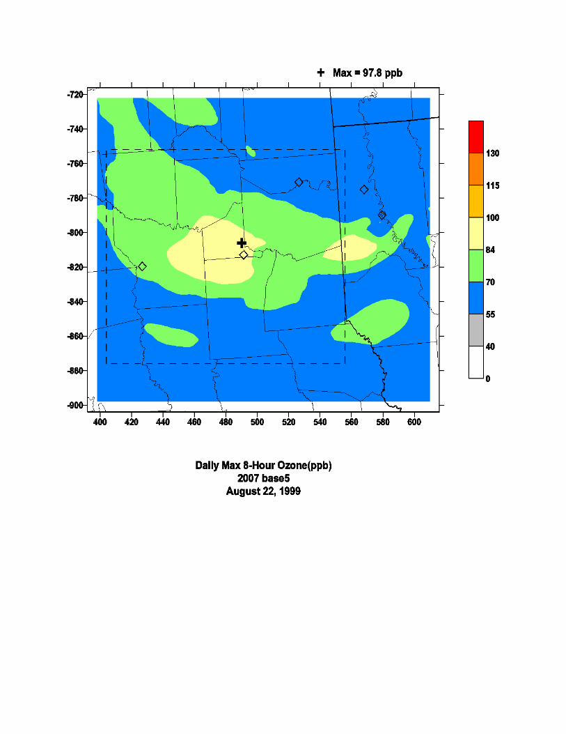

Appendix E
Time Series of Estimated and Observed 1-Hour and 8-Hour Ozone (ppb)
for AIRS Monitors in the 4-km Grid for the August 15-22, 1999 Episode:
1999 Base Case 7

ETCOG 4-km Grid: Base Case 7 1-Hour Ozone
220150008: Shreveport:A irport
0
50100
150
8/13/99 8/14/99 8/15/99 8/16/99 8/17/99 8/18/99 8/19/99 8/20/99 8/21/99 8/22/99Da te
O3
[ppb
] M inim um to Max imum Ra nge O bser ved P redic ted
220170001: Shreveport:North
0
50
100150
8/13/99 8/14/99 8/15/99 8/16/99 8/17/99 8/18/99 8/19/99 8/20/99 8/21/99 8/22/99Da te
O3
[ppb
] M inim um to Max imum Ra nge O bser ved P redic ted
481830001: CAMS_19:Longview
050
100
150
8/13/99 8/14/99 8/15/99 8/16/99 8/17/99 8/18/99 8/19/99 8/20/99 8/21/99 8/22/99Da te
O3
[ppb
] M inim um to Max imum Ra nge O bser ved P redic ted
483150050: CAMS_50:Marshall
0
50100
150
8/13/99 8/14/99 8/15/99 8/16/99 8/17/99 8/18/99 8/19/99 8/20/99 8/21/99 8/22/99Da te
O3
[ppb
] M inim um to Max imum Ra nge O bser ved P redic ted
484230004: CAMS_86:Tyler
050
100150
8/13/99 8/14/99 8/15/99 8/16/99 8/17/99 8/18/99 8/19/99 8/20/99 8/21/99 8/22/99Da te
O3
[ppb
] M inim um to Max imum Ra nge O bser ved P redic ted
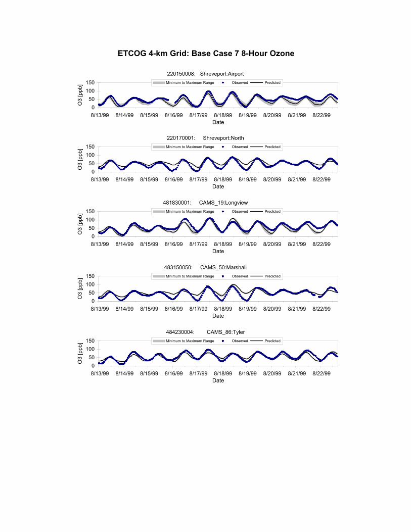
ETCOG 4-km Grid: Base Case 7 8-Hour Ozone
220150008: Shreveport:Airport
050
100150
8/13/99 8/14/99 8/15/99 8/16/99 8/17/99 8/18/99 8/19/99 8/20/99 8/21/99 8/22/99Date
O3
[ppb
] Minimum to Maximum Range Observed Predicted
220170001: Shreveport:North
050
100150
8/13/99 8/14/99 8/15/99 8/16/99 8/17/99 8/18/99 8/19/99 8/20/99 8/21/99 8/22/99Date
O3
[ppb
] Minimum to Maximum Range Observed Predicted
481830001: CAMS_19:Longview
050
100150
8/13/99 8/14/99 8/15/99 8/16/99 8/17/99 8/18/99 8/19/99 8/20/99 8/21/99 8/22/99Date
O3
[ppb
] Minimum to Maximum Range Observed Predicted
483150050: CAMS_50:Marshall
050
100150
8/13/99 8/14/99 8/15/99 8/16/99 8/17/99 8/18/99 8/19/99 8/20/99 8/21/99 8/22/99Date
O3
[ppb
] Minimum to Maximum Range Observed Predicted
484230004: CAMS_86:Tyler
050
100150
8/13/99 8/14/99 8/15/99 8/16/99 8/17/99 8/18/99 8/19/99 8/20/99 8/21/99 8/22/99Date
O3
[ppb
] Minimum to Maximum Range Observed Predicted

Appendix F
Time Series of Estimated and Observed 1-Hour Ozone (ppb)
for AIRS Monitors in the 12-km Grid for the August 15-22, 1999 Episode:
1999 Base Case 7

ETCOG 12-km Grid: Base Case 7
50350005: 50350005
050
100150
8/13/99 8/14/99 8/15/99 8/16/99 8/17/99 8/18/99 8/19/99 8/20/99 8/21/99 8/22/99Date
O3
[ppb
] Minimum to Maximum Range Observed Predicted
50970001: 50970001
050
100150
8/13/99 8/14/99 8/15/99 8/16/99 8/17/99 8/18/99 8/19/99 8/20/99 8/21/99 8/22/99Date
O3
[ppb
] Minimum to Maximum Range Observed Predicted
51190007: 51190007
050
100150
8/13/99 8/14/99 8/15/99 8/16/99 8/17/99 8/18/99 8/19/99 8/20/99 8/21/99 8/22/99Date
O3
[ppb
] Minimum to Maximum Range Observed Predicted
51191002: 51191002
050
100150
8/13/99 8/14/99 8/15/99 8/16/99 8/17/99 8/18/99 8/19/99 8/20/99 8/21/99 8/22/99Date
O3
[ppb
] Minimum to Maximum Range Observed Predicted
220050004: 220050004
050
100150
8/13/99 8/14/99 8/15/99 8/16/99 8/17/99 8/18/99 8/19/99 8/20/99 8/21/99 8/22/99Date
O3
[ppb
] Minimum to Maximum Range Observed Predicted
220110002: 220110002
050
100150
8/13/99 8/14/99 8/15/99 8/16/99 8/17/99 8/18/99 8/19/99 8/20/99 8/21/99 8/22/99Date
O3
[ppb
] Minimum to Maximum Range Observed Predicted

ETCOG 12-km Grid: Base Case 7
220150008: 220150008
0
50100
150
8/13/99 8/14/99 8/15/99 8/16/99 8/17/99 8/18/99 8/19/99 8/20/99 8/21/99 8/22/99Da te
O3
[ppb
] M inim um to Max imum Ra nge O bser ved P redic ted
220170001: 220170001
0
50
100150
8/13/99 8/14/99 8/15/99 8/16/99 8/17/99 8/18/99 8/19/99 8/20/99 8/21/99 8/22/99Da te
O3
[ppb
] M inim um to Max imum Ra nge O bser ved P redic ted
220190008: 220190008
050
100
150
8/13/99 8/14/99 8/15/99 8/16/99 8/17/99 8/18/99 8/19/99 8/20/99 8/21/99 8/22/99Da te
O3
[ppb
] M inim um to Max imum Ra nge O bser ved P redic ted
220190009: 220190009
0
50100
150
8/13/99 8/14/99 8/15/99 8/16/99 8/17/99 8/18/99 8/19/99 8/20/99 8/21/99 8/22/99Da te
O3
[ppb
] M inim um to Max imum Ra nge O bser ved P redic ted
220330003: 220330003
050
100150
8/13/99 8/14/99 8/15/99 8/16/99 8/17/99 8/18/99 8/19/99 8/20/99 8/21/99 8/22/99Da te
O3
[ppb
] M inim um to Max imum Ra nge O bser ved P redic ted
220330009: 220330009
0
50100
150
8/13/99 8/14/99 8/15/99 8/16/99 8/17/99 8/18/99 8/19/99 8/20/99 8/21/99 8/22/99Da te
O3
[ppb
] M inim um to Max imum Ra nge O bser ved P redic ted

ETCOG 12-km Grid: Base Case 7
220330013: 220330013
0
50100
150
8/13/99 8/14/99 8/15/99 8/16/99 8/17/99 8/18/99 8/19/99 8/20/99 8/21/99 8/22/99Da te
O3
[ppb
] M inim um to Max imum Ra nge O bser ved P redic ted
220331001: 220331001
0
50
100150
8/13/99 8/14/99 8/15/99 8/16/99 8/17/99 8/18/99 8/19/99 8/20/99 8/21/99 8/22/99Da te
O3
[ppb
] M inim um to Max imum Ra nge O bser ved P redic ted
220430001: 220430001
050
100
150
8/13/99 8/14/99 8/15/99 8/16/99 8/17/99 8/18/99 8/19/99 8/20/99 8/21/99 8/22/99Da te
O3
[ppb
] M inim um to Max imum Ra nge O bser ved P redic ted
220470002: 220470002
0
50100
150
8/13/99 8/14/99 8/15/99 8/16/99 8/17/99 8/18/99 8/19/99 8/20/99 8/21/99 8/22/99Da te
O3
[ppb
] M inim um to Max imum Ra nge O bser ved P redic ted
220470007: 220470007
050
100150
8/13/99 8/14/99 8/15/99 8/16/99 8/17/99 8/18/99 8/19/99 8/20/99 8/21/99 8/22/99Da te
O3
[ppb
] M inim um to Max imum Ra nge O bser ved P redic ted
220470009: 220470009
0
50100
150
8/13/99 8/14/99 8/15/99 8/16/99 8/17/99 8/18/99 8/19/99 8/20/99 8/21/99 8/22/99Da te
O3
[ppb
] M inim um to Max imum Ra nge O bser ved P redic ted

ETCOG 12-km Grid: Base Case 7
220511001: 220511001
050
100150
8/13/99 8/14/99 8/15/99 8/16/99 8/17/99 8/18/99 8/19/99 8/20/99 8/21/99 8/22/99Date
O3
[ppb
] Minimum to Maximum Range Observed Predicted
220550005: 220550005
050
100150
8/13/99 8/14/99 8/15/99 8/16/99 8/17/99 8/18/99 8/19/99 8/20/99 8/21/99 8/22/99Date
O3
[ppb
] Minimum to Maximum Range Observed Predicted
220570002: 220570002
050
100150
8/13/99 8/14/99 8/15/99 8/16/99 8/17/99 8/18/99 8/19/99 8/20/99 8/21/99 8/22/99Date
O3
[ppb
] Minimum to Maximum Range Observed Predicted
220630002: 220630002
050
100150
8/13/99 8/14/99 8/15/99 8/16/99 8/17/99 8/18/99 8/19/99 8/20/99 8/21/99 8/22/99Date
O3
[ppb
] Minimum to Maximum Range Observed Predicted
220710012: 220710012
050
100150
8/13/99 8/14/99 8/15/99 8/16/99 8/17/99 8/18/99 8/19/99 8/20/99 8/21/99 8/22/99Date
O3
[ppb
] Minimum to Maximum Range Observed Predicted
220730004: 220730004
050
100150
8/13/99 8/14/99 8/15/99 8/16/99 8/17/99 8/18/99 8/19/99 8/20/99 8/21/99 8/22/99Date
O3
[ppb
] Minimum to Maximum Range Observed Predicted

ETCOG 12-km Grid: Base Case 7
220770001: 220770001
050
100150
8/13/99 8/14/99 8/15/99 8/16/99 8/17/99 8/18/99 8/19/99 8/20/99 8/21/99 8/22/99Date
O3
[ppb
] Minimum to Maximum Range Observed Predicted
220870002: 220870002
050
100150
8/13/99 8/14/99 8/15/99 8/16/99 8/17/99 8/18/99 8/19/99 8/20/99 8/21/99 8/22/99Date
O3
[ppb
] Minimum to Maximum Range Observed Predicted
220890003: 220890003
050
100150
8/13/99 8/14/99 8/15/99 8/16/99 8/17/99 8/18/99 8/19/99 8/20/99 8/21/99 8/22/99Date
O3
[ppb
] Minimum to Maximum Range Observed Predicted
220930002: 220930002
050
100150
8/13/99 8/14/99 8/15/99 8/16/99 8/17/99 8/18/99 8/19/99 8/20/99 8/21/99 8/22/99Date
O3
[ppb
] Minimum to Maximum Range Observed Predicted
220950002: 220950002
050
100150
8/13/99 8/14/99 8/15/99 8/16/99 8/17/99 8/18/99 8/19/99 8/20/99 8/21/99 8/22/99Date
O3
[ppb
] Minimum to Maximum Range Observed Predicted
221010003: 221010003
050
100150
8/13/99 8/14/99 8/15/99 8/16/99 8/17/99 8/18/99 8/19/99 8/20/99 8/21/99 8/22/99Date
O3
[ppb
] Minimum to Maximum Range Observed Predicted

ETCOG 12-km Grid: Base Case 7
221210001: 221210001
0
50100
150
8/13/99 8/14/99 8/15/99 8/16/99 8/17/99 8/18/99 8/19/99 8/20/99 8/21/99 8/22/99Da te
O3
[ppb
] M inim um to Max imum Ra nge O bser ved P redic ted
280010004: 280010004
0
50
100150
8/13/99 8/14/99 8/15/99 8/16/99 8/17/99 8/18/99 8/19/99 8/20/99 8/21/99 8/22/99Da te
O3
[ppb
] M inim um to Max imum Ra nge O bser ved P redic ted
280110001: 280110001
050
100
150
8/13/99 8/14/99 8/15/99 8/16/99 8/17/99 8/18/99 8/19/99 8/20/99 8/21/99 8/22/99Da te
O3
[ppb
] M inim um to Max imum Ra nge O bser ved P redic ted
280330002: 280330002
0
50100
150
8/13/99 8/14/99 8/15/99 8/16/99 8/17/99 8/18/99 8/19/99 8/20/99 8/21/99 8/22/99Da te
O3
[ppb
] M inim um to Max imum Ra nge O bser ved P redic ted
280450001: 280450001
050
100150
8/13/99 8/14/99 8/15/99 8/16/99 8/17/99 8/18/99 8/19/99 8/20/99 8/21/99 8/22/99Da te
O3
[ppb
] M inim um to Max imum Ra nge O bser ved P redic ted
280490010: 280490010
0
50100
150
8/13/99 8/14/99 8/15/99 8/16/99 8/17/99 8/18/99 8/19/99 8/20/99 8/21/99 8/22/99Da te
O3
[ppb
] M inim um to Max imum Ra nge O bser ved P redic ted

ETCOG 12-km Grid: Base Case 7
280810005: 280810005
0
50100
150
8/13/99 8/14/99 8/15/99 8/16/99 8/17/99 8/18/99 8/19/99 8/20/99 8/21/99 8/22/99Da te
O3
[ppb
] M inim um to Max imum Ra nge O bser ved P redic ted
280890002: 280890002
0
50
100150
8/13/99 8/14/99 8/15/99 8/16/99 8/17/99 8/18/99 8/19/99 8/20/99 8/21/99 8/22/99Da te
O3
[ppb
] M inim um to Max imum Ra nge O bser ved P redic ted
281490004: 281490004
050
100
150
8/13/99 8/14/99 8/15/99 8/16/99 8/17/99 8/18/99 8/19/99 8/20/99 8/21/99 8/22/99Da te
O3
[ppb
] M inim um to Max imum Ra nge O bser ved P redic ted
400270049: 400270049
0
50100
150
8/13/99 8/14/99 8/15/99 8/16/99 8/17/99 8/18/99 8/19/99 8/20/99 8/21/99 8/22/99Da te
O3
[ppb
] M inim um to Max imum Ra nge O bser ved P redic ted
400310647: 400310647
050
100150
8/13/99 8/14/99 8/15/99 8/16/99 8/17/99 8/18/99 8/19/99 8/20/99 8/21/99 8/22/99Da te
O3
[ppb
] M inim um to Max imum Ra nge O bser ved P redic ted
400670670: 400670670
0
50100
150
8/13/99 8/14/99 8/15/99 8/16/99 8/17/99 8/18/99 8/19/99 8/20/99 8/21/99 8/22/99Da te
O3
[ppb
] M inim um to Max imum Ra nge O bser ved P redic ted
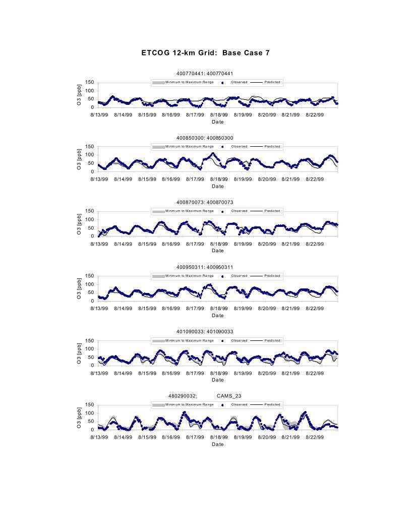
ETCOG 12-km Grid: Base Case 7
400770441: 400770441
0
50100
150
8/13/99 8/14/99 8/15/99 8/16/99 8/17/99 8/18/99 8/19/99 8/20/99 8/21/99 8/22/99Da te
O3
[ppb
] M inim um to Max imum Ra nge O bser ved P redic ted
400850300: 400850300
0
50
100150
8/13/99 8/14/99 8/15/99 8/16/99 8/17/99 8/18/99 8/19/99 8/20/99 8/21/99 8/22/99Da te
O3
[ppb
] M inim um to Max imum Ra nge O bser ved P redic ted
400870073: 400870073
050
100
150
8/13/99 8/14/99 8/15/99 8/16/99 8/17/99 8/18/99 8/19/99 8/20/99 8/21/99 8/22/99Da te
O3
[ppb
] M inim um to Max imum Ra nge O bser ved P redic ted
400950311: 400950311
0
50100
150
8/13/99 8/14/99 8/15/99 8/16/99 8/17/99 8/18/99 8/19/99 8/20/99 8/21/99 8/22/99Da te
O3
[ppb
] M inim um to Max imum Ra nge O bser ved P redic ted
401090033: 401090033
050
100150
8/13/99 8/14/99 8/15/99 8/16/99 8/17/99 8/18/99 8/19/99 8/20/99 8/21/99 8/22/99Da te
O3
[ppb
] M inim um to Max imum Ra nge O bser ved P redic ted
480290032: CAMS_23
0
50100
150
8/13/99 8/14/99 8/15/99 8/16/99 8/17/99 8/18/99 8/19/99 8/20/99 8/21/99 8/22/99Da te
O3
[ppb
] M inim um to Max imum Ra nge O bser ved P redic ted

ETCOG 12-km Grid: Base Case 7
480290052: CAMS_58
0
50100
150
8/13/99 8/14/99 8/15/99 8/16/99 8/17/99 8/18/99 8/19/99 8/20/99 8/21/99 8/22/99Da te
O3
[ppb
] M inim um to Max imum Ra nge O bser ved P redic ted
480290055: CAMS_678
0
50
100150
8/13/99 8/14/99 8/15/99 8/16/99 8/17/99 8/18/99 8/19/99 8/20/99 8/21/99 8/22/99Da te
O3
[ppb
] M inim um to Max imum Ra nge O bser ved P redic ted
480290059: CAMS_59
050
100
150
8/13/99 8/14/99 8/15/99 8/16/99 8/17/99 8/18/99 8/19/99 8/20/99 8/21/99 8/22/99Da te
O3
[ppb
] M inim um to Max imum Ra nge O bser ved P redic ted
480391003: CAMS_11
0
50100
150
8/13/99 8/14/99 8/15/99 8/16/99 8/17/99 8/18/99 8/19/99 8/20/99 8/21/99 8/22/99Da te
O3
[ppb
] M inim um to Max imum Ra nge O bser ved P redic ted
480550062: CAMS_62
050
100150
8/13/99 8/14/99 8/15/99 8/16/99 8/17/99 8/18/99 8/19/99 8/20/99 8/21/99 8/22/99Da te
O3
[ppb
] M inim um to Max imum Ra nge O bser ved P redic ted
480850005: CAMS_31
0
50100
150
8/13/99 8/14/99 8/15/99 8/16/99 8/17/99 8/18/99 8/19/99 8/20/99 8/21/99 8/22/99Da te
O3
[ppb
] M inim um to Max imum Ra nge O bser ved P redic ted

ETCOG 12-km Grid: Base Case 7
481130075: CAMS_63
0
50100
150
8/13/99 8/14/99 8/15/99 8/16/99 8/17/99 8/18/99 8/19/99 8/20/99 8/21/99 8/22/99Da te
O3
[ppb
] M inim um to Max imum Ra nge O bser ved P redic ted
481210034: CAMS_56
0
50
100150
8/13/99 8/14/99 8/15/99 8/16/99 8/17/99 8/18/99 8/19/99 8/20/99 8/21/99 8/22/99Da te
O3
[ppb
] M inim um to Max imum Ra nge O bser ved P redic ted
481390015: CAMS_94
050
100
150
8/13/99 8/14/99 8/15/99 8/16/99 8/17/99 8/18/99 8/19/99 8/20/99 8/21/99 8/22/99Da te
O3
[ppb
] M inim um to Max imum Ra nge O bser ved P redic ted
481670014: CAMS_34
0
50100
150
8/13/99 8/14/99 8/15/99 8/16/99 8/17/99 8/18/99 8/19/99 8/20/99 8/21/99 8/22/99Da te
O3
[ppb
] M inim um to Max imum Ra nge O bser ved P redic ted
481671002: CAMS_10
050
100150
8/13/99 8/14/99 8/15/99 8/16/99 8/17/99 8/18/99 8/19/99 8/20/99 8/21/99 8/22/99Da te
O3
[ppb
] M inim um to Max imum Ra nge O bser ved P redic ted
481830001: CAMS_19
0
50100
150
8/13/99 8/14/99 8/15/99 8/16/99 8/17/99 8/18/99 8/19/99 8/20/99 8/21/99 8/22/99Da te
O3
[ppb
] M inim um to Max imum Ra nge O bser ved P redic ted

ETCOG 12-km Grid: Base Case 7
482010024: CAMS_8
050
100150
8/13/99 8/14/99 8/15/99 8/16/99 8/17/99 8/18/99 8/19/99 8/20/99 8/21/99 8/22/99Date
O3
[ppb
] Minimum to Maximum Range Observed Predicted
482010029: CAMS_26
050
100150
8/13/99 8/14/99 8/15/99 8/16/99 8/17/99 8/18/99 8/19/99 8/20/99 8/21/99 8/22/99Date
O3
[ppb
] Minimum to Maximum Range Observed Predicted
482010055: CAMS_53
050
100150
8/13/99 8/14/99 8/15/99 8/16/99 8/17/99 8/18/99 8/19/99 8/20/99 8/21/99 8/22/99Date
O3
[ppb
] Minimum to Maximum Range Observed Predicted
482450009: CAMS_2
050
100150
8/13/99 8/14/99 8/15/99 8/16/99 8/17/99 8/18/99 8/19/99 8/20/99 8/21/99 8/22/99Date
O3
[ppb
] Minimum to Maximum Range Observed Predicted
482450011: CAMS_28
050
100150
8/13/99 8/14/99 8/15/99 8/16/99 8/17/99 8/18/99 8/19/99 8/20/99 8/21/99 8/22/99Date
O3
[ppb
] Minimum to Maximum Range Observed Predicted
482450102: CAMS_643
050
100150
8/13/99 8/14/99 8/15/99 8/16/99 8/17/99 8/18/99 8/19/99 8/20/99 8/21/99 8/22/99Date
O3
[ppb
] Minimum to Maximum Range Observed Predicted
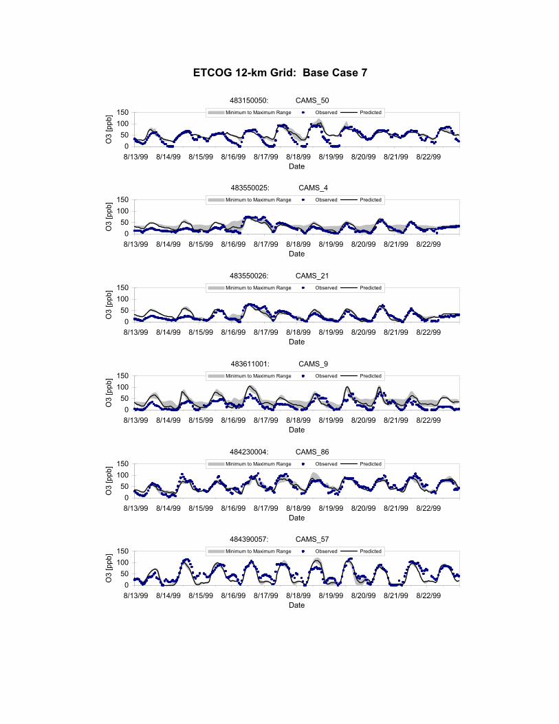
ETCOG 12-km Grid: Base Case 7
483150050: CAMS_50
050
100150
8/13/99 8/14/99 8/15/99 8/16/99 8/17/99 8/18/99 8/19/99 8/20/99 8/21/99 8/22/99Date
O3
[ppb
] Minimum to Maximum Range Observed Predicted
483550025: CAMS_4
050
100150
8/13/99 8/14/99 8/15/99 8/16/99 8/17/99 8/18/99 8/19/99 8/20/99 8/21/99 8/22/99Date
O3
[ppb
] Minimum to Maximum Range Observed Predicted
483550026: CAMS_21
050
100150
8/13/99 8/14/99 8/15/99 8/16/99 8/17/99 8/18/99 8/19/99 8/20/99 8/21/99 8/22/99Date
O3
[ppb
] Minimum to Maximum Range Observed Predicted
483611001: CAMS_9
050
100150
8/13/99 8/14/99 8/15/99 8/16/99 8/17/99 8/18/99 8/19/99 8/20/99 8/21/99 8/22/99Date
O3
[ppb
] Minimum to Maximum Range Observed Predicted
484230004: CAMS_86
050
100150
8/13/99 8/14/99 8/15/99 8/16/99 8/17/99 8/18/99 8/19/99 8/20/99 8/21/99 8/22/99Date
O3
[ppb
] Minimum to Maximum Range Observed Predicted
484390057: CAMS_57
050
100150
8/13/99 8/14/99 8/15/99 8/16/99 8/17/99 8/18/99 8/19/99 8/20/99 8/21/99 8/22/99Date
O3
[ppb
] Minimum to Maximum Range Observed Predicted

ETCOG 12-km Grid: Base Case 7
484391002: CAMS_13
050
100150
8/13/99 8/14/99 8/15/99 8/16/99 8/17/99 8/18/99 8/19/99 8/20/99 8/21/99 8/22/99Date
O3
[ppb
] Minimum to Maximum Range Observed Predicted
484392003: CAMS_17
050
100150
8/13/99 8/14/99 8/15/99 8/16/99 8/17/99 8/18/99 8/19/99 8/20/99 8/21/99 8/22/99Date
O3
[ppb
] Minimum to Maximum Range Observed Predicted
484530014: CAMS_3
050
100150
8/13/99 8/14/99 8/15/99 8/16/99 8/17/99 8/18/99 8/19/99 8/20/99 8/21/99 8/22/99Date
O3
[ppb
] Minimum to Maximum Range Observed Predicted
484530020: CAMS_38
050
100150
8/13/99 8/14/99 8/15/99 8/16/99 8/17/99 8/18/99 8/19/99 8/20/99 8/21/99 8/22/99Date
O3
[ppb
] Minimum to Maximum Range Observed Predicted
484690003: CAMS_87
050
100150
8/13/99 8/14/99 8/15/99 8/16/99 8/17/99 8/18/99 8/19/99 8/20/99 8/21/99 8/22/99Date
O3
[ppb
] Minimum to Maximum Range Observed Predicted
484790016: CAMS_44
050
100150
8/13/99 8/14/99 8/15/99 8/16/99 8/17/99 8/18/99 8/19/99 8/20/99 8/21/99 8/22/99Date
O3
[ppb
] Minimum to Maximum Range Observed Predicted

APPENDIX G
Scatter Plots of Estimated and Observed 1-Hour Ozone (ppb) for AIRS Monitors in the 4-km Grid for the
August 15-22, 1999 Episode: 1999 Base Case 7
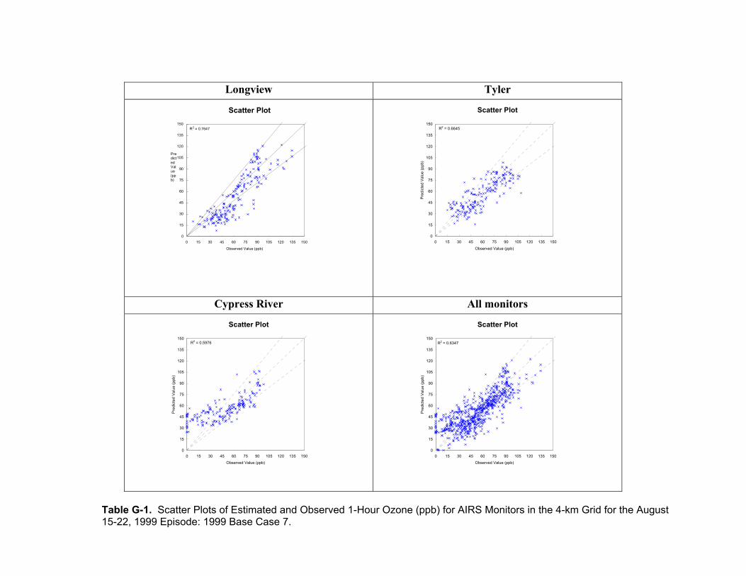
Longview Tyler
Scatter Plot
R 2 = 0.7647
0 15 30 45 60 75 90
105 120 135 150
0 15 30 45 60 75 90 105 120 135 150
Observed Value (ppb)
Predicted Value (ppb)
Scatter Plot
R2 = 0.6645
0
15
30
45
60
75
90
105
120
135
150
0 15 30 45 60 75 90 105 120 135 150
Observed Value (ppb)
Pre
dict
ed V
alue
(ppb
)
Cypress River All monitors
Scatter Plot
R2 = 0.5976
0
15
30
45
60
75
90
105
120
135
150
0 15 30 45 60 75 90 105 120 135 150Observed Value (ppb)
Pre
dict
ed V
alue
(ppb
)
Scatter Plot
R2 = 0.6347
0
15
30
45
60
75
90
105
120
135
150
0 15 30 45 60 75 90 105 120 135 150Observed Value (ppb)
Pre
dict
ed V
alue
(ppb
)
Table G-1. Scatter Plots of Estimated and Observed 1-Hour Ozone (ppb) for AIRS Monitors in the 4-km Grid for the August 15-22, 1999 Episode: 1999 Base Case 7.

APPENDIX H
Scatter Plots and Quantile-Quantile Plots of Daily Maximum 1-Hour Ozone (ppb) for AIRS Monitors in Northeast Texas for the
August 15-22, 1999 Episode: 1999 Base Case 7

Longview Tyler Nearest daily maximum 1-Hour ozone.Subregion = ETCOG FINE2 Longview
0
15
30
45
60
75
90
105
120
135
150
0 15 30 45 60 75 90 105 120 135 150Observed Ozone (ppb)
Pre
dict
ed O
zone
(ppb
)
r2=0.8727
Nearest daily maximum 1-Hour ozone.Subregion = ETCOG FINE2 Tyler
0
15
30
45
60
75
90
105
120
135
150
0 15 30 45 60 75 90 105 120 135 150Observed Ozone (ppb)
Pre
dict
ed O
zone
(ppb
)
r2=0.8419
Cypress River All monitors Nearest daily maximum 1-Hour ozone.
Subregion = ETCOG FINE2 Cypress River
0
15
30
45
60
75
90
105
120
135
150
0 15 30 45 60 75 90 105 120 135 150Observed Ozone (ppb)
Pre
dict
ed O
zone
(ppb
)
r2=0.9748
Nearest daily maximum 1-Hour ozone.Subregion = ETCOG FINE2 Txbox
0
15
30
45
60
75
90
105
120
135
150
0 15 30 45 60 75 90 105 120 135 150Observed Ozone (ppb)
Pre
dict
ed O
zone
(ppb
)
r2=0.9131O - - O shows quantiles
Table H-1. Scatter Plots and Quantile-Quantile Plots of daily Maximum 1-Hour Ozone (ppb) for AIRS Monitors in Northeast Texas for the August 15-22, 1999 Episode: 1999 Base Case 7. Quantiles are not shown for individual monitors because there are two few data.

APPENDIX I
Model Performance Statistics for 1-Hour Ozone (ppb) for AIRS Monitors in the 4-km Grid for the August 15-22,
1999 Episode: 1999 Base Case 7

Table I-1. Model performance statistics for 1-hour ozone for all AIRS monitors in Northeast Texas.
Stats 99/08/15 99/08/16 99/08/17 99/08/18 99/08/19 99/08/20 99/08/21 99/08/22Bias (normalized) -4.5% -18.0% -6.9% 12.6% -6.4% -12.3% -17.4% -4.0%Bias (fractional) -5.4% -21.6% -8.1% 11.1% -7.7% -13.6% -21.3% -6.1%Error (normalized) 9.5% 19.7% 13.4% 14.9% 12.2% 13.3% 18.6% 14.1%Error (fractional) 10.1% 23.1% 14.0% 13.4% 13.1% 14.5% 22.4% 15.5% Table I-2. Model performance statistics for 1-hour ozone by monitor over all days.
Stats Longview Cypress River Tyler Bias (normalized) -4.4% -6.8% -5.6%Bias (fractional) -7.5% -8.3% -6.9%Error (normalized) 17.3% 13.5% 12.4%Error (fractional) 19.3% 14.1% 13.2% A cutoff of 60ppb was used.

APPENDIX J
Scatter Plots of Estimated and Observed 8-Hour Ozone (ppb) for AIRS Monitors in the 4-km Grid for the
August 15-22, 1999 Episode: 1999 Base Case 7

Longview Tyler
Scatter Plot
R2 = 0.7864
0
15
30
45
60
75
90
105
120
135
150
0 15 30 45 60 75 90 105 120 135 150
Observed Value (ppb)
Pre
dict
ed V
alue
(ppb
)
Scatter Plot
R2 = 0.7023
0
15
30
45
60
75
90
105
120
135
150
0 15 30 45 60 75 90 105 120 135 150
Observed Value (ppb)
Pre
dict
ed V
alue
(ppb
)
Cypress River All monitors
Scatter Plots
R2 = 0.5513
0
15
30
45
60
75
90
105
120
135
150
0 15 30 45 60 75 90 105 120 135 150
Observed Value (ppb)
Pre
dict
ed V
alue
(ppb
)
Scatter Plot
R2 = 0.627
0
15
30
45
60
75
90
105
120
135
150
0 15 30 45 60 75 90 105 120 135 150
Observed Value (ppb)
Pre
dict
ed V
alue
(ppb
)
Table J-1. Scatter Plots of Estimated and Observed 1-Hour Ozone (ppb) for AIRS Monitors in the 4-km Grid for the August 15-22, 1999 Episode: 1999 Base Case 7.
Appendix K:
Quantile-Quantile Plots of 8-Hour Ozone (ppb) for AIRS Monitors in the 4-km Grid for the
August 15-22, 1999 Episode: 1999 Base Case 7

Longview Tyler
Nearest daily maximum 8-Hour ozone.Subregion = ETCOG FINE2 Longview
0
15
30
45
60
75
90
105
120
135
150
0 15 30 45 60 75 90 105 120 135 150Observed Ozone (ppb)
Pre
dict
ed O
zone
(ppb
)
r2=0.7672
Nearest daily maximum 8-Hour ozone.Subregion = ETCOG FINE2 Tyler
0
15
30
45
60
75
90
105
120
135
150
0 15 30 45 60 75 90 105 120 135 150Observed Ozone (ppb)
Pre
dict
ed O
zone
(ppb
)
r2=0.8936
Cypress River All monitors Nearest daily maximum 8-Hour ozone.
Subregion = ETCOG FINE2 Cypress River
0
15
30
45
60
75
90
105
120
135
150
0 15 30 45 60 75 90 105 120 135 150Observed Ozone (ppb)
Pre
dict
ed O
zone
(ppb
)
r2=0.9262
Nearest daily maximum 8-Hour ozone.Subregion = ETCOG FINE2 Txbox
0
15
30
45
60
75
90
105
120
135
150
0 15 30 45 60 75 90 105 120 135 150Observed Ozone (ppb)
Pre
dict
ed O
zone
(ppb
)
r2=0.8785O - - O shows quantiles
Table K-1. Scatter plots and Quantile-Quantile Plots of daily maximum 8-hour Ozone (ppb) for AIRS Monitors in Northeast Texas for the August 15-22, 1999 Episode: 1999 Base Case 7. Quantiles are not shown for individual monitors because there are two few data.

Appendix L:
Model Performance Statistics for 8-Hour Ozone (ppb) for AIRS Monitors in Northeast Texas for the
August 15-22, 1999 Episode: 1999 Base Case 7
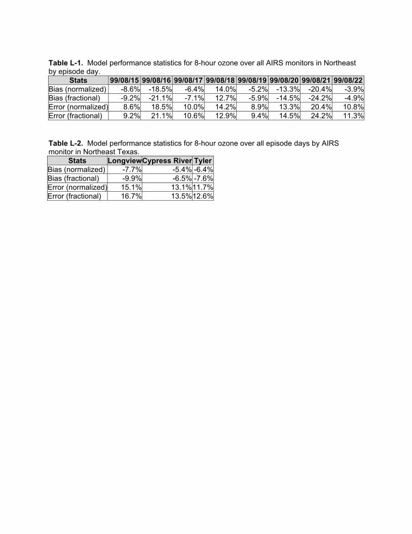
Table L-1. Model performance statistics for 8-hour ozone over all AIRS monitors in Northeast by episode day.
Stats 99/08/15 99/08/16 99/08/17 99/08/18 99/08/19 99/08/20 99/08/21 99/08/22Bias (normalized) -8.6% -18.5% -6.4% 14.0% -5.2% -13.3% -20.4% -3.9%Bias (fractional) -9.2% -21.1% -7.1% 12.7% -5.9% -14.5% -24.2% -4.9%Error (normalized) 8.6% 18.5% 10.0% 14.2% 8.9% 13.3% 20.4% 10.8%Error (fractional) 9.2% 21.1% 10.6% 12.9% 9.4% 14.5% 24.2% 11.3% Table L-2. Model performance statistics for 8-hour ozone over all episode days by AIRS monitor in Northeast Texas.
Stats LongviewCypress River TylerBias (normalized) -7.7% -5.4% -6.4%Bias (fractional) -9.9% -6.5% -7.6%Error (normalized) 15.1% 13.1%11.7%Error (fractional) 16.7% 13.5%12.6%