preliminaryinforumweb.umd.edu/papers/conferences/2002/thaipads.pdf · 2 consumption sectors i and...

THE DEMAND SYSTEM FOR PRIVATE CONSUMPTION OF THAILAND: AN EMPIRICAL ANALYSIS

- Preliminary -

By

Somprawin Manprasert

Department of Economics

University of Maryland

[email protected]

December, 2001

1

1. INTRODUCTION

The objective of this paper is to examine the demand system for the private consumption

of Thailand during 1961-1998 and to build the consumption part of the Interindustry

Dynamic Macroeconomic Model (INTERDYME) for Thai economy. The methodology is

to apply the Perhaps Adequate Demand System (PADS) suggested by Almon (1996) to

estimate 33 private consumption sectors of Thailand. The paper consists of four main

sections: In the second section, there will be a specification of the functional form. Data

source and the estimation procedure will also be mentioned. Next, the results of the

estimation and discussions will be in section 3. The last section will be a conclusion and

final remarks.

2. FUNCTIONAL FORM, DATA SOURCE, AND ESTIMATION PROCEDURE

In order to help readers to understand the results of the estimation, the functional form

and the meaning of its parameters are briefly discussed as follows:

( )

⋅ ⋅∏P

p

P

p

p

p

P

p(y/P)b+(t)a = (t)x

g

i

-

G

i

-

k

i

s-n

=1k

i

-

iii

gGkki

νµλλ

[1]

where;

∏∏∑

∏∑

=∈

∈

∈

∈ =

n

k

Sk

sk

gk

k

gk

1/

gsk

Gk

k

Gk

1/

Gkkk pPandp

s = P p

s = P

1

, [2]

Equation [1] above represents the PADS functional form. Dependent variable xi on the left-

hand-side is a private consumption in sector i. PG, Pg, and P in equation [2] refer to the price

index of group G, the price index of subgroup g, and a general price level, respectively. Sk is

an expenditure share of product k on total consumption expenditure. pi and pk are prices of

2

consumption sectors i and k , respectively. Finally, t and y are time trend and per capita

income.

ai, bi, λi, µG, and νg are all parameters. The number of λi’s to be estimated equals the

number of consumption sectors. Meanwhile, the numbers of µG and νg are estimated

equal to the numbers of groups and subgroups, respectively. Positive (negative) µG

implies a substitution (complementary) within group G and, similarly, positive (negative)

νg implies a substitution (complementary) within subgroup g.

According to the PADS functional form in equation [1], one may be able to derive its

properties of demand. The own-price elasticity and the cross-price elasticity can easily be

derived from the functional form. Each of these price elasticities will be a function of λi,

µG, and νg. For example, the own-price elasticity of consumption sector i is1;

∑=

−−−=n

kkkiiii ss

1, )21( λλε if i ∉ G and i ∉ g [3]

)1()21(1

, ∑∑∈

=∈

−−−−−=

Gkk

iG

n

kkkii

Giii s

sss µλλε if i ∈ G [4]

)1()1()21(1,

, ∑∑∑∈∈

=∈∈

−−−−−−−=

gkk

ig

Gkk

iG

n

kkkii

giGiii s

s

s

sss νµλλε if i ∈ G and i ∈ g [5]

1 One may derive these equations by taking log in equation [1], differentiating it with respect to ln(pi), and rearranging terms.

3

Equation [3] presents the price elasticity of a sector which is ungrouped. Equation [4]

refers to the price elasticity of a sector which is a member of a group, but not that of a

subgroup. On the other hand, equation [5] represents the price elasticity of a sector which

is member of a group, and that of a subgroup.

The estimates of λi and si are individual; however, µG and νg are common within the

same group and subgroup. Thus, the last two equations of price elasticities indicate that

price elasticities of grouped sectors share common parameters. This is worth mentioning

because it leads to the procedure of constraining the results in this research.

2.3 DATA SOURCE AND THE ESTIMATION PROCEDURE

Sectoral time series of private consumption expenditures and sectoral time series of

prices were obtained from the National Economic and Social Development Board

(NESDB) of Thailand. The time series for real disposable income and population were

also obtained at the same source. The estimation procedure follows the non-linear least

square estimation, using the Marquardt Algorithm to fit the non-linear system. A list of

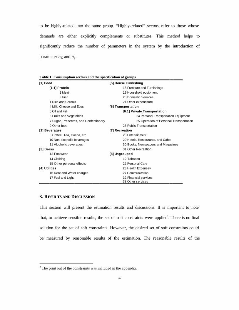
private consumption sectors and the specification of groups and subgroups is presented in

Table 1 below. The specification of the consumption group slightly differs from that of

the National Account, which primarily specifies groups that represent ‘types’ of goods.

Instead, in this study, groups and subgroups were specified such that they represent how

goods were consumed and were related. Certainly, there is a correlation between the

‘type’ of goods being consumed and ‘how’ they were consumed; however, there is not

always a correlation. Therefore, the new classification is similar to the National Account

version, but they are not exact. The intuition here is that we put those sectors which tend

4

to be highly-related into the same group. “Highly-related” sectors refer to those whose

demands are either explicitly complements or substitutes. This method helps to

significantly reduce the number of parameters in the system by the introduction of

parameter µG and νg.

Table 1: Consumption sectors and the specification of groups

[1] Food [5] House Furnishing [1.1] Protein 18 Furniture and Furnishings 2 Meat 19 Household equipment 3 Fish 20 Domestic Services 1 Rice and Cereals 21 Other expenditure 4 Milk, Cheese and Eggs [6] Transportation 5 Oil and Fat [6.1] Private Transportation 6 Fruits and Vegetables 24 Personal Transportation Equipment 7 Sugar, Preserves, and Confectionery 25 Operation of Personal Transportation 9 Other food 26 Public Transportation [2] Beverages [7] Recreation 8 Coffee, Tea, Cocoa, etc. 28 Entertainment 10 Non-alcoholic beverages 29 Hotels, Restaurants, and Cafes 11 Alcoholic beverages 30 Books, Newspapers and Magazines [3] Dress 31 Other Recreation 13 Footwear [8] Ungrouped 14 Clothing 12 Tobacco 15 Other personal effects 22 Personal Care [4] Utilities 23 Health Expenses 16 Rent and Water charges 27 Communication 17 Fuel and Light 32 Financial services 33 Other services

3. RESULTS AND DISCUSSION

This section will present the estimation results and discussions. It is important to note

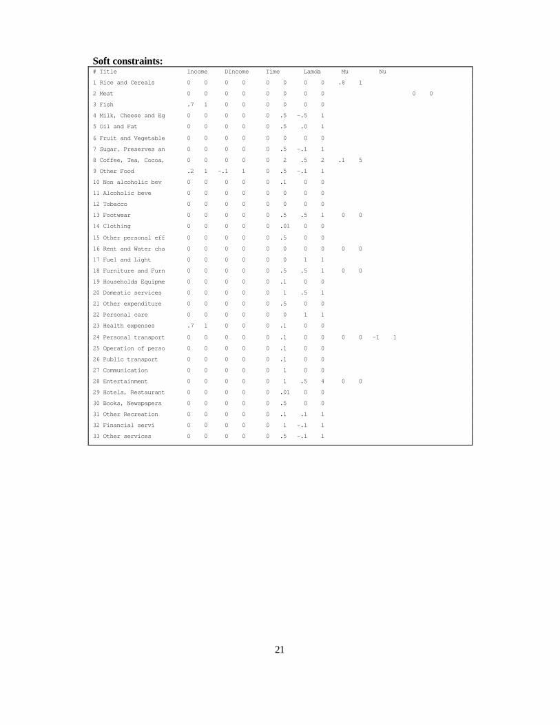
that, to achieve sensible results, the set of soft constraints were applied2. There is no final

solution for the set of soft constraints. However, the desired set of soft constraints could

be measured by reasonable results of the estimation. The reasonable results of the

2 The print out of the constraints was included in the appendix.

5

estimation refer to positive income elasticities in all sectors, negative own-price

elasticities in all sectors, and intuitive values of estimated DInc, µ, and ν.

In addition, the plausible relationship between an estimated income elasticity and a time

trend coefficient for each sector should be maintained. Generally, income variables are

closely related to time trend since they are normally growing through time. However, on

one hand, an estimation sometimes magnifies the effect from a growing income, and

undermines the effect from a time trend. This problem could be recognized by the result

that gives a very high income elasticity but, at the same time, delivers a very negative

time trend coefficient. On the other hand, income variables could also be undermined by

a time trend. This problem is implied by the result that has a low income elasticity and a

highly positive time trend coefficient3.

In order to arrive at the results presented below, soft constraints were applied to each

consumption sector, one-by-one. The constraining procedure started at sectors that seem

to have the least problem and the least complicated term of price elasticity. That is, I

began the process with ungrouped sectors. Soft constraints were applied, if any requires,

to each of those ungrouped sectors to deliver sensible results mentioned above. Then, the

process continued with sectors that are in a group which has no subgroup. Finally, soft

constraints were applied to sectors that are in a group that contains a subgroup. Certainly,

sectors in subgroups are the last ones that were constrained. This method is particularly

3 See unconstrained results in the appendix. It could be noticed that in the estimation with no soft constraints, there are many sectors exhibit highly positive income elasticities and highly negative time trend coefficients at the same time.

6

helpful for keeping track of how price elasticity of a sector would change after it has been

constrained because price elasticities of sectors that are in the same group are interrelated.

3.1 AN OVERVIEW: THE ANALYSIS AT GROUP LEVELS

The analysis begins with the relationship between demands for goods within each group.

Thirty-three private consumption sectors of Thailand were grouped into seven groups and

two subgroups. Six consumption sectors remained ungrouped. As implied by the PADS

functional form, values of µ and ν indicate whether goods in the group and subgroup,

respectively, are complements or substitutes. As a reminder, a positive µG implies

substitution within group G, while its negative value implies the complementarity. A

similar inference also applies for the value of νg at subgroup level. Table 2 below

presents the estimated values of µ and ν.

Table 2: Estimated values of µµ’s and νν’s

Group µµ Subgroup νν 1. Food 0.71 i. Protein 1.18 2. Beverages 0.27 3. Dress -0.10 4. Utilities -1.11 5. Housing Furnishing 0.85 6. Transportation 0.49 ii. Private Transportation -1.10 7. Recreation -0.23

Within the Food group, the result implies that demands for food are substitutes. The

value of µ1 is positive and equals to 0.71. Interestingly, as the sectors that give a similar

dietary source were further added into a subgroup, namely the Protein subgroup, the

estimated value of ν1 (1.18) shows a stronger substitution effect. According to Table 3

below, the Food group by far has accounted for the largest expenditure share.

7

Particularly, Thai people have spent 24.4% of the total consumption expenditure for their

consumption.

Table 3: Expenditure Shares by Group

Group Share Ungrouped Sectors Share Food 0.244 Tobacco 0.022 Protein (0.070) Personal Care 0.019 Beverages 0.074 Health Expenses 0.074 Dress 0.111 Communication 0.008 Utilities 0.098 Financial Services 0.009 House Furnishing 0.084 Other Services 0.009 Transportation 0.111 Private transportation (0.062) Recreation 0.137 Total 1.000

The second group is Beverages. Similar to those in the Food group, demands for

consumption in this group are also substitutes; however, µ2 (0.27) shows less

substitutions. The explanation could be that some sectors in the Beverages group, such as

alcoholic beverages and coffee, carry some degree of addictive property. Therefore, it

could be possible that substitutions are not as high. In contrast to the Food group, the

expenditure share in Table 3 shows that the Beverages group has accounted for the least

share.

The next group is the Dress group. µ3 (-0.10) shows that demands for consumption in this

group are indeed complements, implying that price decreases in Cloth, for example,

could lead to an increase in consumption in Footwear. Thai people have spent 11.1% of

their consumption share for this group.

Demands for consumption in the Utilities group, show a strong complementarity, in

which estimated µ4 is equivalent to -1.11. Intuitively, this group actually consists of Rent-

8

and-Water sector and Fuel-and-Light sector. A high rent may imply more space and more

luxury, which could cause a higher bill for lighting. Therefore, these sectors could show

high complementarity.

The value of µ5 for the House Furnishing group equals 0.85, which implies substitution

between demands for members of this group. For instance, a relatively higher price of the

Domestic service (a housemaid) could make the consumers buy more Household

equipment (such as electrical appliances, and etc.).

The next group is the Transportation. There is also a Private Transportation subgroup

specified in this group. The value of µ6, which equals to 0.49, implies that private

transportation and public transportation are substitutes. The higher the costs of using

private cars, the more likely that Thai consumers would travel by public transportation.

On the other hand, the value of v2 is negative and is equivalent to -1.10, which indeed

suggests a high complement between the cost of purchasing a car and the cost of running

a car. The last group specified is the Recreation group. The estimated µ7 (-0.23)

indicates a complementarity of demands within this group.

3.2 THE ANALYSIS OF 33 PRIVATE CONSUMPTION SECTORS

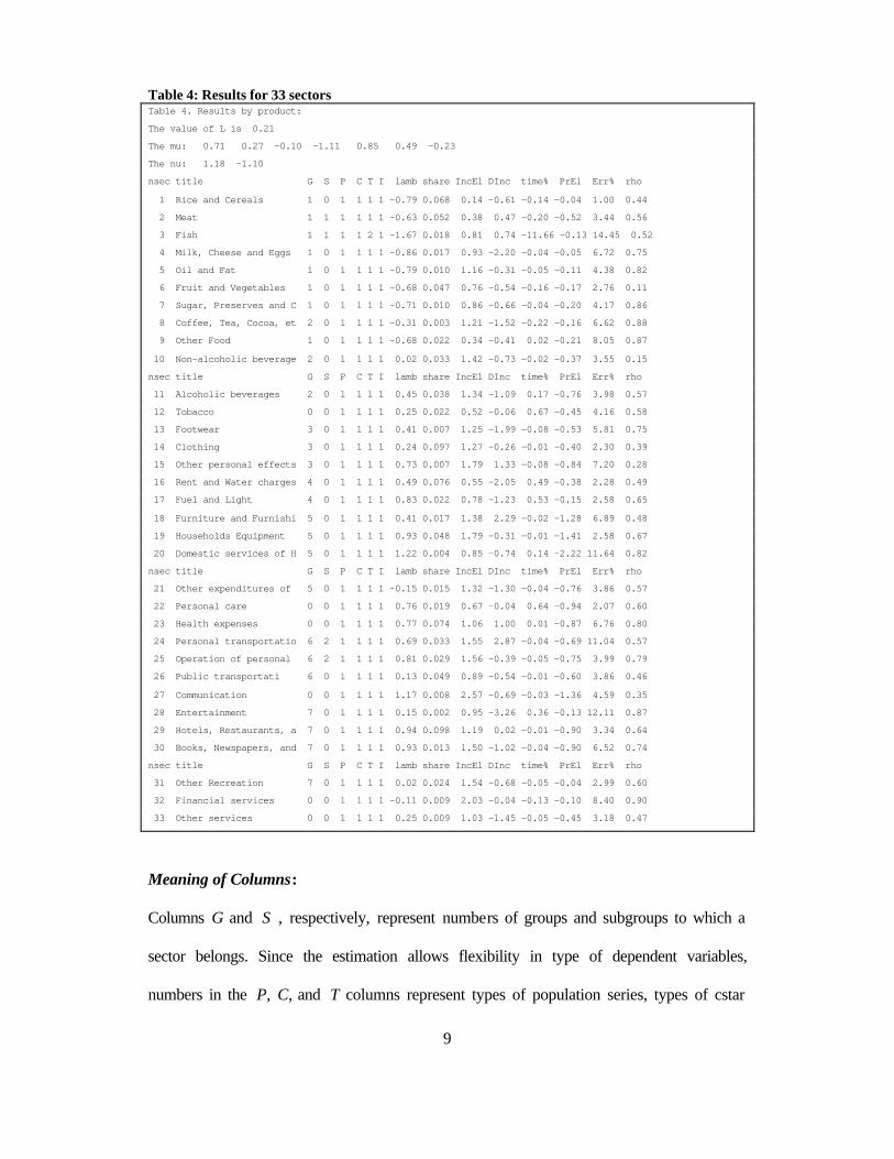
This section will present results of the estimation in detail. The results of all 33 private

consumption sectors will be presented and will be discussed. Table 4 below presents

results of all 33 Thai private consumption sectors:

9

Table 4: Results for 33 sectors Table 4. Results by product:

The value of L is 0.21

The mu: 0.71 0.27 -0.10 -1.11 0.85 0.49 -0.23

The nu: 1.18 -1.10

nsec title G S P C T I lamb share IncEl DInc time% PrEl Err% rho

1 Rice and Cereals 1 0 1 1 1 1 -0.79 0.068 0.14 -0.61 -0.14 -0.04 1.00 0.44

2 Meat 1 1 1 1 1 1 -0.63 0.052 0.38 0.47 -0.20 -0.52 3.44 0.56

3 Fish 1 1 1 1 2 1 -1.67 0.018 0.81 0.74 -11.66 -0.13 14.45 0.52

4 Milk, Cheese and Eggs 1 0 1 1 1 1 -0.86 0.017 0.93 -2.20 -0.04 -0.05 6.72 0.75

5 Oil and Fat 1 0 1 1 1 1 -0.79 0.010 1.16 -0.31 -0.05 -0.11 4.38 0.82

6 Fruit and Vegetables 1 0 1 1 1 1 -0.68 0.047 0.76 -0.54 -0.16 -0.17 2.76 0.11

7 Sugar, Preserves and C 1 0 1 1 1 1 -0.71 0.010 0.86 -0.66 -0.04 -0.20 4.17 0.86

8 Coffee, Tea, Cocoa, et 2 0 1 1 1 1 -0.31 0.003 1.21 -1.52 -0.22 -0.16 6.62 0.88

9 Other Food 1 0 1 1 1 1 -0.68 0.022 0.34 -0.41 0.02 -0.21 8.05 0.87

10 Non-alcoholic beverage 2 0 1 1 1 1 0.02 0.033 1.42 -0.73 -0.02 -0.37 3.55 0.15


11 Alcoholic beverages 2 0 1 1 1 1 0.45 0.038 1.34 -1.09 0.17 -0.76 3.98 0.57

12 Tobacco 0 0 1 1 1 1 0.25 0.022 0.52 -0.06 0.67 -0.45 4.16 0.58

13 Footwear 3 0 1 1 1 1 0.41 0.007 1.25 -1.99 -0.08 -0.53 5.81 0.75

14 Clothing 3 0 1 1 1 1 0.24 0.097 1.27 -0.26 -0.01 -0.40 2.30 0.39

15 Other personal effects 3 0 1 1 1 1 0.73 0.007 1.79 1.33 -0.08 -0.84 7.20 0.28

16 Rent and Water charges 4 0 1 1 1 1 0.49 0.076 0.55 -2.05 0.49 -0.38 2.28 0.49

17 Fuel and Light 4 0 1 1 1 1 0.83 0.022 0.78 -1.23 0.53 -0.15 2.58 0.65

18 Furniture and Furnishi 5 0 1 1 1 1 0.41 0.017 1.38 2.29 -0.02 -1.28 6.89 0.48

19 Households Equipment 5 0 1 1 1 1 0.93 0.048 1.79 -0.31 -0.01 -1.41 2.58 0.67

20 Domestic services of H 5 0 1 1 1 1 1.22 0.004 0.85 -0.74 0.14 -2.22 11.64 0.82


21 Other expenditures of 5 0 1 1 1 1 -0.15 0.015 1.32 -1.30 -0.04 -0.76 3.86 0.57

22 Personal care 0 0 1 1 1 1 0.76 0.019 0.67 -0.04 0.64 -0.94 2.07 0.60

23 Health expenses 0 0 1 1 1 1 0.77 0.074 1.06 1.00 0.01 -0.87 6.76 0.80

24 Personal transportatio 6 2 1 1 1 1 0.69 0.033 1.55 2.87 -0.04 -0.69 11.04 0.57

25 Operation of personal 6 2 1 1 1 1 0.81 0.029 1.56 -0.39 -0.05 -0.75 3.99 0.79

26 Public transportati 6 0 1 1 1 1 0.13 0.049 0.89 -0.54 -0.01 -0.60 3.86 0.46

27 Communication 0 0 1 1 1 1 1.17 0.008 2.57 -0.69 -0.03 -1.36 4.59 0.35

28 Entertainment 7 0 1 1 1 1 0.15 0.002 0.95 -3.26 0.36 -0.13 12.11 0.87

29 Hotels, Restaurants, a 7 0 1 1 1 1 0.94 0.098 1.19 0.02 -0.01 -0.90 3.34 0.64

30 Books, Newspapers, and 7 0 1 1 1 1 0.93 0.013 1.50 -1.02 -0.04 -0.90 6.52 0.74


31 Other Recreation 7 0 1 1 1 1 0.02 0.024 1.54 -0.68 -0.05 -0.04 2.99 0.60

32 Financial services 0 0 1 1 1 1 -0.11 0.009 2.03 -0.04 -0.13 -0.10 8.40 0.90

33 Other services 0 0 1 1 1 1 0.25 0.009 1.03 -1.45 -0.05 -0.45 3.18 0.47

Meaning of Columns:

Columns G and S , respectively, represent numbers of groups and subgroups to which a

sector belongs. Since the estimation allows flexibility in type of dependent variables,

numbers in the P, C, and T columns represent types of population series, types of cstar

10

series (income), and types of time trend series that were used for a sector. In this case,

there is only one type of series for each of population variable and cstar variable.

However, there are two types of time trend variables; a normal time trend variable, which

is simply a series of years, and a special time trend variable (dummy time trend) for the

Fish sector4. Column I indicates the inclusion code, where code ‘1’ refers to a situation

that a sector is price sensitive and price terms were included in the system estimation.

However, if a sector is price insensitive (for example, goods that are paid for by a third

party such as the government), the inclusion code would be ‘0’.

The Lamb and Share columns are estimated λi parameter and expenditure share si for the

consumption sector i. The IncEl column is an implied income elasticity; while, DInc

column represents a ratio of the coefficient on income change to the coefficient on

income variable. Value in the Time% column shows how consumers’ demands change,

with respect to time (1 year passage), holding income and price constant. In other words,

it simply represents changes in consumers’ taste. The next column, PrEl, refers to an

implied price elasticity for each consumption sector. The Err% column corresponds to a

percentage of standard error with respect to the average of the last 5 actual data. Finally,

the Rho is a autocorrelation of the residuals.

Discussion of the Results:

The discussion of results will be taken in the order of groups. The analysis will begin

with the Food group. Finally, some of those ungrouped sectors will be examined.

4 See the appendix for a graph of consumption on Fish and the specification of this special time trend.

11

I. Food Group

There are eight consumption sectors that were specified in the Food group. Two

consumption sectors that are likely to be closely substituted due to their dietary source,

namely Meat and Fish, were further specified into a Protein subgroup. As indicated in

section 3.1, demands for food are substitutes, where µ1 equals to 0.71. Furthermore, Meat

and Fish are highly substituted for each other, as ν1 equals to 1.18. Table 5 below

reproduces estimated results for consumption sectors in the Food group.

Table 5: Results for Food Group nsec title G S P C T I lamb share IncEl DInc time% PrEl Err% rho

1 Rice and Cereals 1 0 1 1 1 1 -0.79 0.068 0.14 -0.61 -0.14 -0.04 1.00 0.44

2 Meat 1 1 1 1 1 1 -0.63 0.052 0.38 0.47 -0.20 -0.52 3.44 0.56

3 Fish 1 1 1 1 2 1 -1.67 0.018 0.81 0.74 -11.66 -0.13 14.45 0.52

4 Milk, Cheese and Eggs 1 0 1 1 1 1 -0.86 0.017 0.93 -2.20 -0.04 -0.05 6.72 0.75

5 Oil and Fat 1 0 1 1 1 1 -0.79 0.010 1.16 -0.31 -0.05 -0.11 4.38 0.82



9 Other Food 1 0 1 1 1 1 -0.68 0.022 0.34 -0.41 0.02 -0.21 8.05 0.87

Note: This table was reproduced from table 4 above.

The expenditure share suggests that Thai people have spent their food budget share

primarily on Rice, Meat, and Fruit-and-vegetables. Particularly, their share are 0.068,

0.052, and 0.047, respectively. Expenditure shares of these three sectors account for more

than half of the share that has been spent on the Food group. Income elasticities also give

us intuitive results. With exception of the Oil-and-fat sector, every member of the Food

group has its income elasticity less than 1, which implies that food is necessary good.

Interestingly, only Meat and Fish have positive DInc values, which equal to 0.47 and

0.74, respectively. This means that Thai consumers would increase their consumption at

higher rate on these sectors, as their incomes increase.

12

Price elasticities also imply sensible results - that is, all price elasticities in these sectors

are less than 1 in absolute term. This property suggests that demands for food are

inelastic to price changes. Finally, time trend coefficients are, in general, close to 0.

However, the special time trend dummy was applied to Fish, and the estimated time trend

coefficient accounts for only a sharp decrease in its consumption during 1982-1991.

Therefore, the highly negative time trend coefficient of Fish is indeed unmistaken5.

II. Beverages Group

There are three consumption sectors specified in this group, namely, Coffee-tea-cocoa,

Non-alcoholic beverages, and Alcoholic beverages. As mentioned in the previous section,

the estimated µ2 suggests that beverages are substitutes. The results for the Beverages

group are presented in table 6 below:

Table 6: Results for Beverages Group nsec title G S P C T I lamb share IncEl DInc time% PrEl Err% rho

8 Coffee, Tea, Cocoa, et 2 0 1 1 1 1 -0.31 0.003 1.21 -1.52 -0.22 -0.16 6.62 0.88




As discussed earlier, Thai consumers have spent only 7.4% of their total consumption

expenditure on this group; however, examining the group in detail gives us a better

picture. Actually, the consumers have spent the least consumption share on the Coffee-

tea-cocoa sector - only 0.3% of the total consumption expenditure. However, Thai people

have spent a relatively large share on alcoholic beverages. The positive time trend

coefficient of this sector also suggests an increase of interest in alcoholic drinks. Income

5 See the plot of consumption on Fish and the technical note in the appendix.

13

elasticities are all greater than 1. Finally, all price elasticities are less than 1 in absolute

terms, implying that the demands for beverages are inelastic.

III. Dress Group

There are three consumption sectors specified in the Dress group: Footwear, Clothing,

and Other personal effects. According to table 2, estimated µ3 (-0.10) implies that these

goods are mild complements. Table 7 below presents the results of this group:

Table 7: Results for Dress Group nsec title G S P C T I lamb share IncEl DInc time% PrEl Err% rho

13 Footwear 3 0 1 1 1 1 0.41 0.007 1.25 -1.99 -0.08 -0.53 5.81 0.75

14 Clothing 3 0 1 1 1 1 0.24 0.097 1.27 -0.26 -0.01 -0.40 2.30 0.39



It is important to point out that Clothing has a very large expenditure share, and actually

it is the second largest share in all sectors. About 9.7% of the total consumption

expenditure has been allocated to Clothing. Indeed, income elasticities indicate that Dress

is a luxury good. Therefore, as per capita income increases, Thai people would

proportionally increase more expenditures on dress. However, the demand for these

sectors seems to be inelastic to prices change, as price elasticities are all less than 1 in

absolute terms. Lastly, time trend coefficients are close to zero.

IV. Utilities Group

Although the Utilities group contains only two consumption sectors, Rents-and-water

charges and Fuel-and-light, this group was specified since these two consumption sectors

share a similar characteristic: consumers must pay these bills monthly. By grouping them

14

together, I anticipated a significant complementarity within this group. This argument

was confirmed by table 2. The estimated µ4 equals to –1.11, which in fact suggests that

goods in this group are strong complements.

Table 8: Results for Utilities Group nsec title G S P C T I lamb share IncEl DInc time% PrEl Err% rho


17 Fuel and Light 4 0 1 1 1 1 0.83 0.022 0.78 -1.23 0.53 -0.15 2.58 0.65


The expenditure share of the Rent-and-water charges is almost four times larger than that

of the Fuel-and-light sector. This is, however, not a surprising outcome. Income

elasticities and price elasticities suggest sensible values. Income elasticities are less than

1 and are equivalent to 0.55 and 0.78, respectively. Therefore, these goods are certainly

necessary. Price elasticities also imply that demands for these goods are inelastic to prices

change. Interestingly, time trend coefficients are both positive. Hence, regardless of

income effect and price effect, Thai people tend to consume more in this group.

V. House Furnishing and Operation Group

There are four consumption sectors in this group: Furniture-and-furnishings, Households

equipment, Domestic services, and Other expenditures. The estimated µ5 presented in

table 2 indicates that consumption goods in this group are substitutes. The detail results

for each sector are shown below:

15

Table 9: Results for House Furnishing Group nsec title G S P C T I lamb share IncEl DInc time% PrEl Err% rho

18 Furniture and Furnishi 5 0 1 1 1 1 0.41 0.017 1.38 2.29 -0.02 -1.28 6.89 0.48


20 Domestic services of H 5 0 1 1 1 1 1.22 0.004 0.85 -0.74 0.14 -2.22 11.64 0.82

21 Other expenditures of 5 0 1 1 1 1 -0.15 0.015 1.32 -1.30 -0.04 -0.76 3.86 0.57


In general, with exception for the Domestic services, income elasticities in other sectors

are all greater than 1. Only price elasticity of the Other expenditures sector, which, in

fact, refers to expenditures on maintenance of other house furnishing goods, shows an

inelastic demand. This result is very intuitive since the demand for purchasing furniture

and equipment could be price elastic; however, once the goods are obtained, demand for

maintaining them could be relatively more inelastic.

Within this group, Thais have made a relatively large expenditure share on Household

equipment. On the other hand, they apportioned the least share to Domestic service (a

housemaid), although a positive time trend coefficient implies that Thais are more

interested in hiring housemaids. Ambiguously, the income elasticity suggests its

necessity, although its demand is rather price elastic.

VI. Transportation Group

There are three consumption sectors in this group: Personal transportation equipment,

Operation of personal transportation, and Public transportation. The subgroup of Private

Transportation was further specified in order to differentiate expenditures on private

cars, which includes the cost of a car and its operational costs, from expenditures on

public transportation. The intuition is that the expenditure on operational costs of a

private car could increase with the cost of a car. The more expensive a car is, the higher

16

its running cost. However, a consumer’s expenditure on public transportation could,

indeed, decrease his expenditure on a private car. For instance, a consumer may prefer to

travel by public bus instead of driving a car if the price of gasoline is relatively high. On

one hand, by specifying subgroup, results are expected to show a high complementarity

between Personal transportation equipment and Operation of the personal transportation.

On the other hand, Private transportation should be substituted for Public transportation.

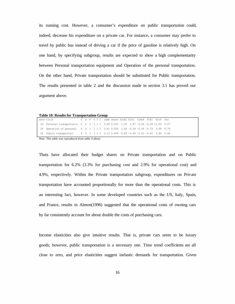
The results presented in table 2 and the discussion made in section 3.1 has proved our

argument above.

Table 10: Results for Transportation Group nsec title G S P C T I lamb share IncEl DInc time% PrEl Err% rho



26 Public transportati 6 0 1 1 1 1 0.13 0.049 0.89 -0.54 -0.01 -0.60 3.86 0.46


Thais have allocated their budget shares on Private transportation and on Public

transportation for 6.2% (3.3% for purchasing cost and 2.9% for operational cost) and

4.9%, respectively. Within the Private transportation subgroup, expenditures on Private

transportation have accounted proportionally for more than the operational costs. This is

an interesting fact, however. In some developed countries such as the US, Italy, Spain,

and France, results in Almon(1996) suggested that the operational costs of owning cars

by far consistently account for about double the costs of purchasing cars.

Income elasticities also give intuitive results. That is, private cars seem to be luxury

goods; however, public transportation is a necessary one. Time trend coefficients are all

close to zero, and price elasticities suggest inelastic demands for transportation. Given

17

this information, it could be inferred that a drastic increase in private transportation

expenditures since mid 90s may mainly come from the growing income per capita of the

Thai population.

VII. Recreation Group

Four consumption sectors were specified in this group: Entertainment, Hotels-restaurants-

cafes, Books-newspapers-magazines, and Other recreation. The primary reason that these

sectors were grouped because they might represent the same type of demand. That is,

they represent consumers’ activities which could lead to an extra utility to consumers.

Thus, they should be luxury goods and they are expected to have income elasticities

greater than 1.

Table 11: Results for Recreation Group nsec title G S P C T I lamb share IncEl DInc time% PrEl Err% rho

28 Entertainment 7 0 1 1 1 1 0.15 0.002 0.95 -3.26 0.36 -0.13 12.11 0.87

29 Hotels, Restaurants, a 7 0 1 1 1 1 0.94 0.098 1.19 0.02 -0.01 -0.90 3.34 0.64


31 Other Recreation 7 0 1 1 1 1 0.02 0.024 1.54 -0.68 -0.05 -0.04 2.99 0.60


Recall that demands for the goods within this group are complements, although not very

strong. Yet, one might question how this complementarity could be explained by real life

situations. The interpretation is straightforward. For example, one situation might be

where a person goes to a movie theater after dining out. It is also worth mentioning that

Hotels-restaurants-cafes has accounted for the highest consumption share in all sectors.

Income elasticities support the argument made earlier - recreation seems to be a luxury

good, and only Entertainment sector has income elasticity less than 1. Moreover, the time

18

trend coefficient suggests that Thais have been interested more in entertainment

activities. Lastly, all price elasticities are less than 1 in absolute terms.

Ungrouped Sectors

There are six consumption sectors that remain ungrouped: Tobacco, Personal care, Health

expenses, Communication, Financial services, and Other services. However, only some

interesting properties of these products will be discussed. First, income elasticity of

Tobacco equals 0.52. Therefore, Tobacco seems to be a necessary good, as it proves its

addictive property. Price elasticity also implies its inelastic demand. Sadly, the time trend

coefficient is positive and equals 0.67. Thus, the taste of Thai people has shifted toward

tobacco products.

Table 12: Results for Ungrouped Sectors nsec title G S P C T I lamb share IncEl DInc time% PrEl Err% rho

12 Tobacco 0 0 1 1 1 1 0.25 0.022 0.52 -0.06 0.67 -0.45 4.16 0.58

22 Personal care 0 0 1 1 1 1 0.76 0.019 0.67 -0.04 0.64 -0.94 2.07 0.60

23 Health expenses 0 0 1 1 1 1 0.77 0.074 1.06 1.00 0.01 -0.87 6.76 0.80

27 Communication 0 0 1 1 1 1 1.17 0.008 2.57 -0.69 -0.03 -1.36 4.59 0.35

32 Financial services 0 0 1 1 1 1 -0.11 0.009 2.03 -0.04 -0.13 -0.10 8.40 0.90

33 Other services 0 0 1 1 1 1 0.25 0.009 1.03 -1.45 -0.05 -0.45 3.18 0.47


Communication is also an interesting sector, although its expenditure share is relatively

small. This product seems to be a luxury good as its income elasticity shows a strong

positive value (2.57). The demand for communication products is also responsive to price

changes. Indeed, the time trend parameter is very close to zero. In fact, these results

suggest that a sharp decrease in communication prices during 1987-1990 and a growing

per capita income are responsible for a major explanation of the skyrocketing

expenditures on communication during past decades.

19

4. CONCLUSION AND FINAL REMARKS

This study gives an understanding of the demands for private consumption in Thailand

during 1961-1998. It conveys information about the trends of consumers’ tastes and their

reactions against income and price changes. In short, the Food group has accounted for

the largest consumption share over the past 38 years. However, for an individual sector,

Thai people have spent the largest proportions on Hotels-restaurants-cafes, Clothing, and

Rice, respectively. Whereas the smallest consumption sector, in terms of a size of the

share, is the Entertainment sector.

Most of sectors have income elasticities greater than 1; however, sectors that show low

income elasticities primarily are food products. The sector that is most sensitive to

income changes is Communication. Generally speaking, time trend coefficients are

negative and close to zero. Sadly, however, some positive time trend coefficients occur in

Alcoholic beverages and Tobacco consumption sectors. This implication should lead to a

revision of the government’s role in a public campaign, or even on a tax policy for these

consumption sectors.

Finally, further extensions could be made in order to gain more understanding of private

consumption behavior in Thailand. Particularly, usage of the total income series and

nation-wide consumption series could be misleading if income is not well-distributed

among the Thai population. It is of particular interest to conduct estimations regarding

different ranges of income classes. Certainly, availability of data would be the next major

constraint for the research.

20

APPENDIX

Unconstrained Results: Table 1. Results by product:

The value of L is 0.15

The mu: 0.84 -0.82 -0.67 -1.31 1.42 0.51 0.47

The nu: 1.81 -0.95


1 Rice and Cereals 1 0 1 1 1 1 -0.87 0.068 0.13 -1.07 -0.09 -0.00 1.09 0.53

2 Meat 1 1 1 1 1 1 -0.77 0.052 0.51 0.30 -0.96 -0.60 3.73 0.45

3 Fish 1 1 1 1 1 1 -2.94 0.018 0.76 -1.20 -6.03 0.57 18.87 0.58

4 Milk, Cheese and Eggs 1 0 1 1 1 1 -1.98 0.017 1.70 -0.89 -2.10 0.98 5.00 0.31

5 Oil and Fat 1 0 1 1 1 1 -1.38 0.010 2.08 -0.32 -2.40 0.40 5.00 0.68



8 Coffee, Tea, Cocoa, et 2 0 1 1 1 1 -0.24 0.003 2.65 -0.87 -4.58 0.87 7.81 0.76

9 Other Food 1 0 1 1 1 1 -1.41 0.022 0.28 -2.57 0.91 0.43 5.52 0.60




12 Tobacco 0 0 1 1 1 1 0.75 0.022 0.59 -1.34 -0.09 -0.87 3.33 0.56

13 Footwear 3 0 1 1 1 1 0.44 0.007 1.94 -1.64 -2.12 0.04 6.05 0.69

14 Clothing 3 0 1 1 1 1 0.31 0.097 1.21 -0.21 -0.00 -0.32 2.17 0.28



17 Fuel and Light 4 0 1 1 1 1 1.43 0.022 0.54 -0.96 1.01 -0.51 3.03 0.70

18 Furniture and Furnishi 5 0 1 1 1 1 -1.29 0.017 2.93 0.54 -4.36 -0.04 5.81 0.28


20 Domestic services of H 5 0 1 1 1 1 -1.78 0.004 -0.43 -1.33 3.37 0.26 9.04 0.79


21 Other expenditures of 5 0 1 1 1 1 1.41 0.015 1.06 -1.01 0.00 -2.70 3.53 0.39

22 Personal care 0 0 1 1 1 1 -1.50 0.019 1.76 -0.54 -1.30 1.28 3.54 0.68

23 Health expenses 0 0 1 1 1 1 1.21 0.074 1.43 0.49 -0.81 -1.19 5.91 0.81



26 Purchased transportati 6 0 1 1 1 1 0.22 0.049 0.97 -0.83 -0.14 -0.64 3.57 0.56

27 Communication 0 0 1 1 1 1 0.98 0.008 4.81 -0.76 -8.49 -1.12 3.34 0.24

28 Entertainment 7 0 1 1 1 1 1.23 0.002 0.45 -3.33 -4.06 -1.83 16.78 0.82

29 Hotels, Restaurants, a 7 0 1 1 1 1 0.64 0.098 1.19 0.21 0.09 -0.80 2.66 0.60



31 Other Recreation 7 0 1 1 1 1 -0.69 0.024 1.54 -0.59 -0.44 0.12 2.22 0.33

32 Financial services 0 0 1 1 1 1 3.21 0.009 3.48 -0.04 -5.25 -3.31 4.48 0.60

33 Other services 0 0 1 1 1 1 -0.10 0.009 0.93 -0.98 -0.05 -0.05 2.79 0.53

21

Soft constraints: # Title Income DIncome Time Lamda Mu Nu

1 Rice and Cereals 0 0 0 0 0 0 0 0 .8 1

2 Meat 0 0 0 0 0 0 0 0 0 0

3 Fish .7 1 0 0 0 0 0 0

4 Milk, Cheese and Eg 0 0 0 0 0 .5 -.5 1

5 Oil and Fat 0 0 0 0 0 .5 .0 1

6 Fruit and Vegetable 0 0 0 0 0 0 0 0

7 Sugar, Preserves an 0 0 0 0 0 .5 -.1 1

8 Coffee, Tea, Cocoa, 0 0 0 0 0 2 .5 2 .1 5

9 Other Food .2 1 -.1 1 0 .5 -.1 1

10 Non alcoholic bev 0 0 0 0 0 .1 0 0

11 Alcoholic beve 0 0 0 0 0 0 0 0

12 Tobacco 0 0 0 0 0 0 0 0

13 Footwear 0 0 0 0 0 .5 .5 1 0 0

14 Clothing 0 0 0 0 0 .01 0 0

15 Other personal eff 0 0 0 0 0 .5 0 0

16 Rent and Water cha 0 0 0 0 0 0 0 0 0 0

17 Fuel and Light 0 0 0 0 0 0 1 1

18 Furniture and Furn 0 0 0 0 0 .5 .5 1 0 0

19 Households Equipme 0 0 0 0 0 .1 0 0

20 Domestic services 0 0 0 0 0 1 .5 1

21 Other expenditure 0 0 0 0 0 .5 0 0

22 Personal care 0 0 0 0 0 0 1 1

23 Health expenses .7 1 0 0 0 .1 0 0

24 Personal transport 0 0 0 0 0 .1 0 0 0 0 -1 1

25 Operation of perso 0 0 0 0 0 .1 0 0

26 Public transport 0 0 0 0 0 .1 0 0

27 Communication 0 0 0 0 0 1 0 0

28 Entertainment 0 0 0 0 0 1 .5 4 0 0

29 Hotels, Restaurant 0 0 0 0 0 .01 0 0

30 Books, Newspapers 0 0 0 0 0 .5 0 0

31 Other Recreation 0 0 0 0 0 .1 .1 1

32 Financial servi 0 0 0 0 0 1 -.1 1

33 Other services 0 0 0 0 0 .5 -.1 1

22

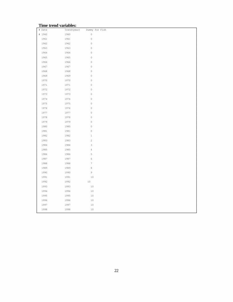
Time trend variables: # Date Trend(year) Dummy for Fish

# 1960 1960 0

1961 1961 0

1962 1962 0

1963 1963 0

1964 1964 0

1965 1965 0

1966 1966 0

1967 1967 0

1968 1968 0

1969 1969 0

1970 1970 0

1971 1971 0

1972 1972 0

1973 1973 0

1974 1974 0

1975 1975 0

1976 1976 0

1977 1977 0

1978 1978 0

1979 1979 0

1980 1980 0

1981 1981 0

1982 1982 1

1983 1983 2

1984 1984 3

1985 1985 4

1986 1986 5

1987 1987 6

1988 1988 7

1989 1989 8

1990 1990 9

1991 1991 10

1992 1992 10

1993 1993 10

1994 1994 10

1995 1995 10

1996 1996 10

1997 1997 10

1998 1998 10

23

Historical plot of Fish consumption per capita and its price:

3. Fish 3. Fish P r i c e v s . C o n s u m p t i o n p e r c a p i t a

8 0 5

5 4 2

2 7 9

1 .7

0 .9

0 .1

1 9 6 0 1 9 6 5 1 9 7 0 1 9 7 5 1 9 8 0 1 9 8 5 1 9 9 0 1 9 9 5

pcepc3 ppc3

Technical note: Fish sector has been using the special time trend variable. According to

the plot, it can be noticed that consumption per capita for Fish did not seem to have an

explicit relationship with its price. Using a normal time trend contributed to a strong

positive price elasticity. Therefore, resolve this problem, the special time trend that runs

only during 1982-1991 was specified.

24

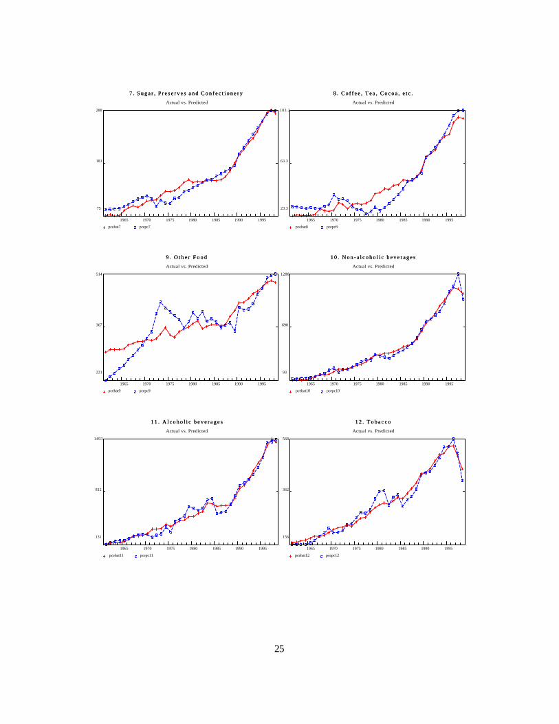
Graphs of fitted values:

1 . R i c e a n d C e r e a l s 1 . R i c e a n d C e r e a l s

Actual vs. Predicted

1244

1165

1086

1965 1970 1975 1980 1985 1990 1995

pcehat1 pcepc1

2 . M e a t 2 . M e a t


1071

796

520

1965 1970 1975 1980 1985 1990 1995

pcehat2 pcepc2

3 . F ish 3 . F ish


789

532

276

1965 1970 1975 1980 1985 1990 1995

pcehat3 pcepc3

4 . M i l k , C h e e s e a n d E g g s 4 . M i l k , C h e e s e a n d E g g s


597

373

150

1965 1970 1975 1980 1985 1990 1995

pcehat4 pcepc4

5 . O i l a n d F a t 5 . O i l a n d F a t


298

167

36

1965 1970 1975 1980 1985 1990 1995

pcehat5 pcepc5

6 . F r u i t a n d V e g e t a b l e s 6 . F r u i t a n d V e g e t a b l e s


1192

843

493

1965 1970 1975 1980 1985 1990 1995

pcehat6 pcepc6

25

7 . S u g a r , P r e s e r v e s a n d C o n f e c t i o n e r y 7 . S u g a r , P r e s e r v e s a n d C o n f e c t i o n e r y


288

181

75

1965 1970 1975 1980 1985 1990 1995

pcehat7 pcepc7

8 . C o f f e e , T e a , C o c o a , e t c . 8 . C o f f e e , T e a , C o c o a , e t c .


103.3

63.3

23.3

1965 1970 1975 1980 1985 1990 1995

pcehat8 pcepc8

9 . O t h e r F o o d 9 . O t h e r F o o d


514

367

221

1965 1970 1975 1980 1985 1990 1995

pcehat9 pcepc9

1 0 . N o n - a l c o h o l i c b e v e r a g e s 1 0 . N o n - a l c o h o l i c b e v e r a g e s


1288

690

93

1965 1970 1975 1980 1985 1990 1995

pcehat10 pcepc10

1 1 . A l c o h o l i c b e v e r a g e s 1 1 . A l c o h o l i c b e v e r a g e s


1493

812

131

1965 1970 1975 1980 1985 1990 1995

pcehat11 pcepc11

1 2 . T o b a c c o 1 2 . T o b a c c o


568

362

156

1965 1970 1975 1980 1985 1990 1995

pcehat12 pcepc12

26

1 3 . F o o t w e a r 1 3 . F o o t w e a r


258

156

54

1965 1970 1975 1980 1985 1990 1995

pcehat13 pcepc13

1 4 . C l o t h i n g 1 4 . C l o t h i n g


2684

1525

367

1965 1970 1975 1980 1985 1990 1995

pcehat14 pcepc14

1 5 . O t h e r p e r s o n a l e f f e c t s 1 5 . O t h e r p e r s o n a l e f f e c t s


501

257

12

1965 1970 1975 1980 1985 1990 1995

pcehat15 pcepc15

1 6 . R e n t a n d W a t e r c h a r g e s 1 6 . R e n t a n d W a t e r c h a r g e s


2122

1444

767

1965 1970 1975 1980 1985 1990 1995

pcehat16 pcepc16

1 7 . F u e l a n d L i g h t 1 7 . F u e l a n d L i g h t


690

430

171

1965 1970 1975 1980 1985 1990 1995

pcehat17 pcepc17

1 8 . F u r n i t u r e a n d F u r n i s h i n g s 1 8 . F u r n i t u r e a n d F u r n i s h i n g s


642

326

11

1965 1970 1975 1980 1985 1990 1995

pcehat18 pcepc18

27

1 9 . H o u s e h o l d s E q u i p m e n t 1 9 . H o u s e h o l d s E q u i p m e n t


2135

1077

18

1965 1970 1975 1980 1985 1990 1995

pcehat19 pcepc19

2 0 . D o m e s t i c s e r v i c e s o f H o u s e h o l d o p e r a t i o n 2 0 . D o m e s t i c s e r v i c e s o f H o u s e h o l d o p e r a t i o n


78.7

52.5

26.3

1965 1970 1975 1980 1985 1990 1995

pcehat20 pcepc20

2 1 . O t h e r e x p e n d i t u r e s o f H o u s e h o l d o p e r a t i o n 2 1 . O t h e r e x p e n d i t u r e s o f H o u s e h o l d o p e r a t i o n


524

297

70

1965 1970 1975 1980 1985 1990 1995

pcehat21 pcepc21

2 2 . P e r s o n a l c a r e 2 2 . P e r s o n a l c a r e


531

313

96

1965 1970 1975 1980 1985 1990 1995

pcehat22 pcepc22

2 3 . H e a l t h e x p e n s e s 2 3 . H e a l t h e x p e n s e s


1700

896

91

1965 1970 1975 1980 1985 1990 1995

pcehat23 pcepc23

2 4 . P e r s o n a l t r a n s p o r t a t i o n e q u i p m e n t 2 4 . P e r s o n a l t r a n s p o r t a t i o n e q u i p m e n t


1832

903

-27

1965 1970 1975 1980 1985 1990 1995

pcehat24 pcepc24

28

2 5 . O p e r a t i o n o f p e r s o n a l t r a n s p o r t a t i o n e q u i p m e n t 2 5 . O p e r a t i o n o f p e r s o n a l t r a n s p o r t a t i o n e q u i p m e n t


1235

626

16

1965 1970 1975 1980 1985 1990 1995

pcehat25 pcepc25

2 6 . P u b l i c t r a n s p o r t a t i o n 2 6 . P u b l i c t r a n s p o r t a t i o n


1289

914

539

1965 1970 1975 1980 1985 1990 1995

pcehat26 pcepc26

2 7 . C o m m u n i c a t i o n 2 7 . C o m m u n i c a t i o n


850

412

-26

1965 1970 1975 1980 1985 1990 1995

pcehat27 pcepc27

2 8 . E n t e r t a i n m e n t 2 8 . E n t e r t a i n m e n t


84.9

48.7

12.5

1965 1970 1975 1980 1985 1990 1995

pcehat28 pcepc28

2 9 . H o t e l s , R e s t a u r a n t s , a n d C a f e s 2 9 . H o t e l s , R e s t a u r a n t s , a n d C a f e s


2305

1312

319

1965 1970 1975 1980 1985 1990 1995

pcehat29 pcepc29

3 0 . B o o k s , N e w s p a p e r s , a n d M a g a z i n e s 3 0 . B o o k s , N e w s p a p e r s , a n d M a g a z i n e s


444

258

72

1965 1970 1975 1980 1985 1990 1995

pcehat30 pcepc30

29

3 1 . O t h e r R e c r e a t i o n 3 1 . O t h e r R e c r e a t i o n


814

419

23

1965 1970 1975 1980 1985 1990 1995

pcehat31 pcepc31

3 2 . F i n a n c i a l s e r v i c e s 3 2 . F i n a n c i a l s e r v i c e s


400

193

-15

1965 1970 1975 1980 1985 1990 1995

pcehat32 pcepc32

3 3 . O t h e r s e r v i c e s 3 3 . O t h e r s e r v i c e s


252

159

66

1965 1970 1975 1980 1985 1990 1995

pcehat33 pcepc33

preliminaryinforumweb.umd.edu/papers/conferences/2002/thaipads.pdf · 2 consumption sectors i and...

Documents