p nas: direct neural architecture s task and hardware

Published as a conference paper at ICLR 2019

PROXYLESSNAS: DIRECT NEURAL ARCHITECTURESEARCH ON TARGET TASK AND HARDWARE

Han Cai, Ligeng Zhu, Song HanMassachusetts Institute of Technology{hancai, ligeng, songhan}@mit.edu

ABSTRACT

Neural architecture search (NAS) has a great impact by automatically designingeffective neural network architectures. However, the prohibitive computationaldemand of conventional NAS algorithms (e.g. 104 GPU hours) makes it difficultto directly search the architectures on large-scale tasks (e.g. ImageNet). Differen-tiable NAS can reduce the cost of GPU hours via a continuous representation ofnetwork architecture but suffers from the high GPU memory consumption issue(grow linearly w.r.t. candidate set size). As a result, they need to utilize proxytasks, such as training on a smaller dataset, or learning with only a few blocks,or training just for a few epochs. These architectures optimized on proxy tasksare not guaranteed to be optimal on the target task. In this paper, we presentProxylessNAS that can directly learn the architectures for large-scale target tasksand target hardware platforms. We address the high memory consumption issueof differentiable NAS and reduce the computational cost (GPU hours and GPUmemory) to the same level of regular training while still allowing a large candi-date set. Experiments on CIFAR-10 and ImageNet demonstrate the effectivenessof directness and specialization. On CIFAR-10, our model achieves 2.08% testerror with only 5.7M parameters, better than the previous state-of-the-art architec-ture AmoebaNet-B, while using 6× fewer parameters. On ImageNet, our modelachieves 3.1% better top-1 accuracy than MobileNetV2, while being 1.2× fasterwith measured GPU latency. We also apply ProxylessNAS to specialize neuralarchitectures for hardware with direct hardware metrics (e.g. latency) and provideinsights for efficient CNN architecture design.1

1 INTRODUCTION

Neural architecture search (NAS) has demonstrated much success in automating neural network ar-chitecture design for various deep learning tasks, such as image recognition (Zoph et al., 2018; Caiet al., 2018a; Liu et al., 2018a; Zhong et al., 2018) and language modeling (Zoph & Le, 2017). De-spite the remarkable results, conventional NAS algorithms are prohibitively computation-intensive,requiring to train thousands of models on the target task in a single experiment. Therefore, directlyapplying NAS to a large-scale task (e.g. ImageNet) is computationally expensive or impossible,which makes it difficult for making practical industry impact. As a trade-off, Zoph et al. (2018)propose to search for building blocks on proxy tasks, such as training for fewer epochs, startingwith a smaller dataset (e.g. CIFAR-10), or learning with fewer blocks. Then top-performing blocksare stacked and transferred to the large-scale target task. This paradigm has been widely adoptedin subsequent NAS algorithms (Liu et al., 2018a;b; Real et al., 2018; Cai et al., 2018b; Liu et al.,2018c; Tan et al., 2018; Luo et al., 2018).

However, these blocks optimized on proxy tasks are not guaranteed to be optimal on the targettask, especially when taking hardware metrics such as latency into consideration. More importantly,to enable transferability, such methods need to search for only a few architectural motifs and thenrepeatedly stack the same pattern, which restricts the block diversity and thereby harms performance.

In this work, we propose a simple and effective solution to the aforementioned limitations, calledProxylessNAS, which directly learns the architectures on the target task and hardware instead of with

1Pretrained models and evaluation code are released at https://github.com/MIT-HAN-LAB/ProxylessNAS.

1

https://github.com/MIT-HAN-LAB/ProxylessNAS


Proxy Task Learner

Target Task &

Hardware

Transfer

(1) Previous proxy-based approach (2) Our proxy-less approach

Architecture

Updates

Architecture

Updates

Target Task &

HardwareLearner

Normal Train NAS Need Meta Controller

Need Proxy

DARTS & One-shotNo Meta Controller

Need Proxy

Proxyless (Ours)No Meta Controller

No Proxy

GPU Hours GPU Memory

Figure 1: ProxylessNAS directly optimizes neural network architectures on target task and hard-ware. Benefiting from the directness and specialization, ProxylessNAS can achieve remarkablybetter results than previous proxy-based approaches. On ImageNet, with only 200 GPU hours (200× fewer than MnasNet (Tan et al., 2018)), our searched CNN model for mobile achieves the samelevel of top-1 accuracy as MobileNetV2 1.4 while being 1.8× faster.

proxy (Figure 1). We also remove the restriction of repeating blocks in previous NAS works (Zophet al., 2018; Liu et al., 2018c) and allow all of the blocks to be learned and specified. To achievethis, we reduce the computational cost (GPU hours and GPU memory) of architecture search to thesame level of regular training in the following ways.

GPU hour-wise, inspired by recent works (Liu et al., 2018c; Bender et al., 2018), we formulateNAS as a path-level pruning process. Specifically, we directly train an over-parameterized networkthat contains all candidate paths (Figure 2). During training, we explicitly introduce architectureparameters to learn which paths are redundant, while these redundant paths are pruned at the end oftraining to get a compact optimized architecture. In this way, we only need to train a single networkwithout any meta-controller (or hypernetwork) during architecture search.

However, naively including all the candidate paths leads to GPU memory explosion (Liu et al.,2018c; Bender et al., 2018), as the memory consumption grows linearly w.r.t. the number of choices.Thus, GPU memory-wise, we binarize the architecture parameters (1 or 0) and force only one pathto be active at run-time, which reduces the required memory to the same level of training a compactmodel. We propose a gradient-based approach to train these binarized parameters based on Bina-ryConnect (Courbariaux et al., 2015). Furthermore, to handle non-differentiable hardware objectives(using latency as an example) for learning specialized network architectures on target hardware, wemodel network latency as a continuous function and optimize it as regularization loss. Addition-ally, we also present a REINFORCE-based (Williams, 1992) algorithm as an alternative strategy tohandle hardware metrics.

In our experiments on CIFAR-10 and ImageNet, benefiting from the directness and specialization,our method can achieve strong empirical results. On CIFAR-10, our model reaches 2.08% test errorwith only 5.7M parameters. On ImageNet, our model achieves 75.1% top-1 accuracy which is 3.1%higher than MobileNetV2 (Sandler et al., 2018) while being 1.2× faster. Our contributions can besummarized as follows:

• ProxylessNAS is the first NAS algorithm that directly learns architectures on the large-scale dataset (e.g. ImageNet) without any proxy while still allowing a large candidate setand removing the restriction of repeating blocks. It effectively enlarged the search spaceand achieved better performance.

• We provide a new path-level pruning perspective for NAS, showing a close connectionbetween NAS and model compression (Han et al., 2016). We save memory consumptionby one order of magnitude by using path-level binarization.

• We propose a novel gradient-based approach (latency regularization loss) for handlinghardware objectives (e.g. latency). Given different hardware platforms: CPU/GPU/Mobile,ProxylessNAS enables hardware-aware neural network specialization that’s exactly opti-mized for the target hardware. To our best knowledge, it is the first work to study special-ized neural network architectures for different hardware architectures.

• Extensive experiments showed the advantage of the directness property and the special-ization property of ProxylessNAS. It achieved state-of-the-art accuracy performances onCIFAR-10 and ImageNet under latency constraints on different hardware platforms (GPU,CPU and mobile phone). We also analyze the insights of efficient CNN models specializedfor different hardware platforms and raise the awareness that specialized neural networkarchitecture is needed on different hardware architectures for efficient inference.

2


2 RELATED WORK

The use of machine learning techniques, such as reinforcement learning or neuro-evolution, to re-place human experts in designing neural network architectures, usually referred to as neural archi-tecture search, has drawn an increasing interest (Zoph & Le, 2017; Liu et al., 2018a;b;c; Cai et al.,2018a;b; Pham et al., 2018; Brock et al., 2018; Bender et al., 2018; Elsken et al., 2017; 2018b; Ka-math et al., 2018). In NAS, architecture search is typically considered as a meta-learning process,and a meta-controller (e.g. a recurrent neural network (RNN)), is introduced to explore a givenarchitecture space with training a network in the inner loop to get an evaluation for guiding explo-ration. Consequently, such methods are computationally expensive to run, especially on large-scaletasks, e.g. ImageNet.

Some recent works (Brock et al., 2018; Pham et al., 2018) try to improve the efficiency of thismeta-learning process by reducing the cost of getting an evaluation. In Brock et al. (2018), a hy-pernetwork is utilized to generate weights for each sampled network and hence can evaluate thearchitecture without training it. Similarly, Pham et al. (2018) propose to share weights among allsampled networks under the standard NAS framework (Zoph & Le, 2017). These methods speedup architecture search by orders of magnitude, however, they require a hypernetwork or an RNNcontroller and mainly focus on small-scale tasks (e.g. CIFAR) rather than large-scale tasks (e.g.ImageNet).

Our work is most closely related to One-Shot (Bender et al., 2018) and DARTS (Liu et al., 2018c),both of which get rid of the meta-controller (or hypernetwork) by modeling NAS as a single trainingprocess of an over-parameterized network that comprises all candidate paths. Specifically, One-Shot trains the over-parameterized network with DropPath (Zoph et al., 2018) that drops out eachpath with some fixed probability. Then they use the pre-trained over-parameterized network toevaluate architectures, which are sampled by randomly zeroing out paths. DARTS additionallyintroduces a real-valued architecture parameter for each path and jointly train weight parametersand architecture parameters via standard gradient descent. However, they suffer from the large GPUmemory consumption issue and hence still need to utilize proxy tasks. In this work, we address thelarge memory issue in these two methods through path binarization.

Another relevant topic is network pruning (Han et al., 2016) that aim to improve the efficiency ofneural networks by removing insignificant neurons (Han et al., 2015) or channels (Liu et al., 2017).Similar to these works, we start with an over-parameterized network and then prune the redundantparts to derive the optimized architecture. The distinction is that they focus on layer-level pruningthat only modifies the filter (or units) number of a layer but can not change the topology of thenetwork, while we focus on learning effective network architectures through path-level pruning. Wealso allow both pruning and growing the number of layers.

3 METHOD

We first describe the construction of the over-parameterized network with all candidate paths, thenintroduce how we leverage binarized architecture parameters to reduce the memory consumptionof training the over-parameterized network to the same level as regular training. We propose agradient-based algorithm to train these binarized architecture parameters. Finally, we present twotechniques to handle non-differentiable objectives (e.g. latency) for specializing neural networks ontarget hardware.

3.1 CONSTRUCTION OF OVER-PARAMETERIZED NETWORK

Denote a neural network as N (e, · · · , en) where ei represents a certain edge in the directed acyclicgraph (DAG). Let O = {oi} be the set of N candidate primitive operations (e.g. convolution, pool-ing, identity, zero, etc). To construct the over-parameterized network that includes any architecturein the search space, instead of setting each edge to be a definite primitive operation, we set eachedge to be a mixed operation that has N parallel paths (Figure 2), denoted as mO. As such, theover-parameterized network can be expressed as N (e = m1

O, · · · , en = mnO).

Given input x, the output of a mixed operation mO is defined based on the outputs of its N paths. InOne-Shot,mO(x) is the sum of {oi(x)}, while in DARTS,mO(x) is weighted sum of {oi(x)}where

3


(1) Update weight parameters

Architecture ParametersBinary Gate (0:prune, 1:keep)

OUTPUT

α β σ … δ1 0 0 … 0

(2) Update architecture parameters

INPUT

α β σ … δ0 1 0 … 0

update

fmap not in memoryfmap in memory

INPUT

CONV 5x5

POOL 3x3

... Weight Parameters

CONV 3x3 Identity CONV

5x5POOL

3x3...Identity

update

CONV 3x3

OUTPUT

Table 1

MIT Red

Trainer Latency Model

Direct measurement:expensive and slow

Latency modeling:cheap, fast and differentiable

MIT Red-1

Learnable Block i - 1

Learnable Block i

……

Learnable Block i + 1

……

INPUT

OUTPUT

...

α β σ … ζCONV

5x5POOL

3x3...CONV

3x3Identity

E[latency] =X

i

E[latencyi]<latexit sha1_base64="lntrwtqgrPO1VSk1eaeyNufWf/Q=">AAACNXicfVDLSsNAFJ34rPUVdelmsAiuSiKCboSiCC5cVLAPaEKYTCft0JkkzEyEEPJTbvwPV7pwoYhbf8FJmoW24oGBwznnMvceP2ZUKst6MRYWl5ZXVmtr9fWNza1tc2e3K6NEYNLBEYtE30eSMBqSjqKKkX4sCOI+Iz1/cln4vXsiJI3CO5XGxOVoFNKAYqS05Jk3Dkdq7PvZVT7ISi54xpAiIU7z3IXn0JEJ9zKaw3+Sha/TntmwmlYJOE/sijRAhbZnPjnDCCechAozJOXAtmLlZkgoihnJ604iSYzwBI3IQNMQcSLdrLw6h4daGcIgEvqFCpbqz4kMcSlT7utksa2c9QrxL2+QqODMzWgYJ8Vx04+ChEEVwaJCOKSCYMVSTRAWVO8K8RgJhJUuuq5LsGdPnifd46ZtNe3bk0broqqjBvbBATgCNjgFLXAN2qADMHgAz+ANvBuPxqvxYXxOowtGNbMHfsH4+gbJva55</latexit><latexit sha1_base64="lntrwtqgrPO1VSk1eaeyNufWf/Q=">AAACNXicfVDLSsNAFJ34rPUVdelmsAiuSiKCboSiCC5cVLAPaEKYTCft0JkkzEyEEPJTbvwPV7pwoYhbf8FJmoW24oGBwznnMvceP2ZUKst6MRYWl5ZXVmtr9fWNza1tc2e3K6NEYNLBEYtE30eSMBqSjqKKkX4sCOI+Iz1/cln4vXsiJI3CO5XGxOVoFNKAYqS05Jk3Dkdq7PvZVT7ISi54xpAiIU7z3IXn0JEJ9zKaw3+Sha/TntmwmlYJOE/sijRAhbZnPjnDCCechAozJOXAtmLlZkgoihnJ604iSYzwBI3IQNMQcSLdrLw6h4daGcIgEvqFCpbqz4kMcSlT7utksa2c9QrxL2+QqODMzWgYJ8Vx04+ChEEVwaJCOKSCYMVSTRAWVO8K8RgJhJUuuq5LsGdPnifd46ZtNe3bk0broqqjBvbBATgCNjgFLXAN2qADMHgAz+ANvBuPxqvxYXxOowtGNbMHfsH4+gbJva55</latexit><latexit sha1_base64="lntrwtqgrPO1VSk1eaeyNufWf/Q=">AAACNXicfVDLSsNAFJ34rPUVdelmsAiuSiKCboSiCC5cVLAPaEKYTCft0JkkzEyEEPJTbvwPV7pwoYhbf8FJmoW24oGBwznnMvceP2ZUKst6MRYWl5ZXVmtr9fWNza1tc2e3K6NEYNLBEYtE30eSMBqSjqKKkX4sCOI+Iz1/cln4vXsiJI3CO5XGxOVoFNKAYqS05Jk3Dkdq7PvZVT7ISi54xpAiIU7z3IXn0JEJ9zKaw3+Sha/TntmwmlYJOE/sijRAhbZnPjnDCCechAozJOXAtmLlZkgoihnJ604iSYzwBI3IQNMQcSLdrLw6h4daGcIgEvqFCpbqz4kMcSlT7utksa2c9QrxL2+QqODMzWgYJ8Vx04+ChEEVwaJCOKSCYMVSTRAWVO8K8RgJhJUuuq5LsGdPnifd46ZtNe3bk0broqqjBvbBATgCNjgFLXAN2qADMHgAz+ANvBuPxqvxYXxOowtGNbMHfsH4+gbJva55</latexit><latexit sha1_base64="lntrwtqgrPO1VSk1eaeyNufWf/Q=">AAACNXicfVDLSsNAFJ34rPUVdelmsAiuSiKCboSiCC5cVLAPaEKYTCft0JkkzEyEEPJTbvwPV7pwoYhbf8FJmoW24oGBwznnMvceP2ZUKst6MRYWl5ZXVmtr9fWNza1tc2e3K6NEYNLBEYtE30eSMBqSjqKKkX4sCOI+Iz1/cln4vXsiJI3CO5XGxOVoFNKAYqS05Jk3Dkdq7PvZVT7ISi54xpAiIU7z3IXn0JEJ9zKaw3+Sha/TntmwmlYJOE/sijRAhbZnPjnDCCechAozJOXAtmLlZkgoihnJ604iSYzwBI3IQNMQcSLdrLw6h4daGcIgEvqFCpbqz4kMcSlT7utksa2c9QrxL2+QqODMzWgYJ8Vx04+ChEEVwaJCOKSCYMVSTRAWVO8K8RgJhJUuuq5LsGdPnifd46ZtNe3bk0broqqjBvbBATgCNjgFLXAN2qADMHgAz+ANvBuPxqvxYXxOowtGNbMHfsH4+gbJva55</latexit>

Loss = LossCE + �1||w||22 + �2E[latency]<latexit sha1_base64="UvM7E2w6lXtW50LPl18+gDN1T4k=">AAACSnicbVBNSxxBEO3ZaGJWTTbJ0UvjIgjCMrMEkktAIoKHHBRcFXbHoaanVht7Puiu0Sy98/ty8eTNH+HFQ0LwYs+4gtEUdPN4VY969eJCSUO+f+21Xs3Nv36z8La9uLT87n3nw8cDk5da4EDkKtdHMRhUMsMBSVJ4VGiENFZ4GJ9t1f3Dc9RG5tk+TQoMUzjJ5FgKIEdFHfiRG/ON139kt7YrvsFHyskTiAI+nV5Mp1H/2PYbnvAnNRutxqSyj3N9PkqBTuPYblfDBurUKiDMxKQKq6jT9Xt+U/wlCGagy2a1G3WuRkkuyhQzEgqMGQZ+QaEFTVIorNqj0mAB4gxOcOhgBima0DbGKr7mmISPc+1eRrxhnyospMZM0thN1k7N815N/q83LGn8NbQyK8r6sIdF41JxynmdK0+kRkFq4gAILZ1XLk5BgyCXftuFEDw/+SU46PcCvxfsfe5ufp/FscBW2CpbZwH7wjbZDttlAybYL3bDfrM/3qV36/317h5GW95M84n9U625e9C6tBw=</latexit><latexit sha1_base64="UvM7E2w6lXtW50LPl18+gDN1T4k=">AAACSnicbVBNSxxBEO3ZaGJWTTbJ0UvjIgjCMrMEkktAIoKHHBRcFXbHoaanVht7Puiu0Sy98/ty8eTNH+HFQ0LwYs+4gtEUdPN4VY969eJCSUO+f+21Xs3Nv36z8La9uLT87n3nw8cDk5da4EDkKtdHMRhUMsMBSVJ4VGiENFZ4GJ9t1f3Dc9RG5tk+TQoMUzjJ5FgKIEdFHfiRG/ON139kt7YrvsFHyskTiAI+nV5Mp1H/2PYbnvAnNRutxqSyj3N9PkqBTuPYblfDBurUKiDMxKQKq6jT9Xt+U/wlCGagy2a1G3WuRkkuyhQzEgqMGQZ+QaEFTVIorNqj0mAB4gxOcOhgBima0DbGKr7mmISPc+1eRrxhnyospMZM0thN1k7N815N/q83LGn8NbQyK8r6sIdF41JxynmdK0+kRkFq4gAILZ1XLk5BgyCXftuFEDw/+SU46PcCvxfsfe5ufp/FscBW2CpbZwH7wjbZDttlAybYL3bDfrM/3qV36/317h5GW95M84n9U625e9C6tBw=</latexit><latexit sha1_base64="UvM7E2w6lXtW50LPl18+gDN1T4k=">AAACSnicbVBNSxxBEO3ZaGJWTTbJ0UvjIgjCMrMEkktAIoKHHBRcFXbHoaanVht7Puiu0Sy98/ty8eTNH+HFQ0LwYs+4gtEUdPN4VY969eJCSUO+f+21Xs3Nv36z8La9uLT87n3nw8cDk5da4EDkKtdHMRhUMsMBSVJ4VGiENFZ4GJ9t1f3Dc9RG5tk+TQoMUzjJ5FgKIEdFHfiRG/ON139kt7YrvsFHyskTiAI+nV5Mp1H/2PYbnvAnNRutxqSyj3N9PkqBTuPYblfDBurUKiDMxKQKq6jT9Xt+U/wlCGagy2a1G3WuRkkuyhQzEgqMGQZ+QaEFTVIorNqj0mAB4gxOcOhgBima0DbGKr7mmISPc+1eRrxhnyospMZM0thN1k7N815N/q83LGn8NbQyK8r6sIdF41JxynmdK0+kRkFq4gAILZ1XLk5BgyCXftuFEDw/+SU46PcCvxfsfe5ufp/FscBW2CpbZwH7wjbZDttlAybYL3bDfrM/3qV36/317h5GW95M84n9U625e9C6tBw=</latexit><latexit sha1_base64="UvM7E2w6lXtW50LPl18+gDN1T4k=">AAACSnicbVBNSxxBEO3ZaGJWTTbJ0UvjIgjCMrMEkktAIoKHHBRcFXbHoaanVht7Puiu0Sy98/ty8eTNH+HFQ0LwYs+4gtEUdPN4VY969eJCSUO+f+21Xs3Nv36z8La9uLT87n3nw8cDk5da4EDkKtdHMRhUMsMBSVJ4VGiENFZ4GJ9t1f3Dc9RG5tk+TQoMUzjJ5FgKIEdFHfiRG/ON139kt7YrvsFHyskTiAI+nV5Mp1H/2PYbnvAnNRutxqSyj3N9PkqBTuPYblfDBurUKiDMxKQKq6jT9Xt+U/wlCGagy2a1G3WuRkkuyhQzEgqMGQZ+QaEFTVIorNqj0mAB4gxOcOhgBima0DbGKr7mmISPc+1eRrxhnyospMZM0thN1k7N815N/q83LGn8NbQyK8r6sIdF41JxynmdK0+kRkFq4gAILZ1XLk5BgyCXftuFEDw/+SU46PcCvxfsfe5ufp/FscBW2CpbZwH7wjbZDttlAybYL3bDfrM/3qV36/317h5GW95M84n9U625e9C6tBw=</latexit>

E[Latency] = ↵⇥ F (conv 3x3)+

� ⇥ F (conv 5x5)+

� ⇥ F (identity)+

......

⇣ ⇥ F (pool 3x3)<latexit sha1_base64="Lm2s03uPUYjMAPu22Qv9NriXYRM=">AAADIHicfVJNb9QwEHXCVwlfWzhysViBipBWSUuBC1IFAnHgUCS2rbSOVo4zm7Xq2JHtVBui8E+48Fe4cAAhuMGvwUnDV7vLSJaeZuZ53jw7KQQ3Ngy/e/6Zs+fOX1i7GFy6fOXqtcH69T2jSs1gzJRQ+iChBgSXMLbcCjgoNNA8EbCfHD5t6/tHoA1X8rWtCohzmkk+44xal5quew9IAhmXNRU8k5A2AcmpnSdJ/ayZdFDn9UtqQbKqifFjfOctsbCw3eQ6ESU0NaGimNMGE8tzMPj5xi8eU/KITLcWW81dfA8TEiwjJ2AddxV5e7H9P7LhWb5sMk9BOjeqP9xRF6vuebNCRKGU6DcICMj0t03TwTAchV3g0yDqwRD1sTsdfCOpYmXudDFBjZlEYWHjmmrLmQBne2mgoOyQZjBxUFInJK47kQ2+7TIpnintjrS4y/7NqGluTJUnrrMVbk7W2uSy2qS0s0dxzWVRti98PGhWCmwVbn8LTrkGZkXlAGWaO62YzammzLo/FTgTopMrnwZ7m6MoHEWv7g93nvR2rKGb6BbaQBF6iHbQC7SLxoh577wP3ifvs//e/+h/8b8et/pez7mB/gn/x09YVgHC</latexit><latexit sha1_base64="Lm2s03uPUYjMAPu22Qv9NriXYRM=">AAADIHicfVJNb9QwEHXCVwlfWzhysViBipBWSUuBC1IFAnHgUCS2rbSOVo4zm7Xq2JHtVBui8E+48Fe4cAAhuMGvwUnDV7vLSJaeZuZ53jw7KQQ3Ngy/e/6Zs+fOX1i7GFy6fOXqtcH69T2jSs1gzJRQ+iChBgSXMLbcCjgoNNA8EbCfHD5t6/tHoA1X8rWtCohzmkk+44xal5quew9IAhmXNRU8k5A2AcmpnSdJ/ayZdFDn9UtqQbKqifFjfOctsbCw3eQ6ESU0NaGimNMGE8tzMPj5xi8eU/KITLcWW81dfA8TEiwjJ2AddxV5e7H9P7LhWb5sMk9BOjeqP9xRF6vuebNCRKGU6DcICMj0t03TwTAchV3g0yDqwRD1sTsdfCOpYmXudDFBjZlEYWHjmmrLmQBne2mgoOyQZjBxUFInJK47kQ2+7TIpnintjrS4y/7NqGluTJUnrrMVbk7W2uSy2qS0s0dxzWVRti98PGhWCmwVbn8LTrkGZkXlAGWaO62YzammzLo/FTgTopMrnwZ7m6MoHEWv7g93nvR2rKGb6BbaQBF6iHbQC7SLxoh577wP3ifvs//e/+h/8b8et/pez7mB/gn/x09YVgHC</latexit><latexit sha1_base64="Lm2s03uPUYjMAPu22Qv9NriXYRM=">AAADIHicfVJNb9QwEHXCVwlfWzhysViBipBWSUuBC1IFAnHgUCS2rbSOVo4zm7Xq2JHtVBui8E+48Fe4cAAhuMGvwUnDV7vLSJaeZuZ53jw7KQQ3Ngy/e/6Zs+fOX1i7GFy6fOXqtcH69T2jSs1gzJRQ+iChBgSXMLbcCjgoNNA8EbCfHD5t6/tHoA1X8rWtCohzmkk+44xal5quew9IAhmXNRU8k5A2AcmpnSdJ/ayZdFDn9UtqQbKqifFjfOctsbCw3eQ6ESU0NaGimNMGE8tzMPj5xi8eU/KITLcWW81dfA8TEiwjJ2AddxV5e7H9P7LhWb5sMk9BOjeqP9xRF6vuebNCRKGU6DcICMj0t03TwTAchV3g0yDqwRD1sTsdfCOpYmXudDFBjZlEYWHjmmrLmQBne2mgoOyQZjBxUFInJK47kQ2+7TIpnintjrS4y/7NqGluTJUnrrMVbk7W2uSy2qS0s0dxzWVRti98PGhWCmwVbn8LTrkGZkXlAGWaO62YzammzLo/FTgTopMrnwZ7m6MoHEWv7g93nvR2rKGb6BbaQBF6iHbQC7SLxoh577wP3ifvs//e/+h/8b8et/pez7mB/gn/x09YVgHC</latexit><latexit sha1_base64="Lm2s03uPUYjMAPu22Qv9NriXYRM=">AAADIHicfVJNb9QwEHXCVwlfWzhysViBipBWSUuBC1IFAnHgUCS2rbSOVo4zm7Xq2JHtVBui8E+48Fe4cAAhuMGvwUnDV7vLSJaeZuZ53jw7KQQ3Ngy/e/6Zs+fOX1i7GFy6fOXqtcH69T2jSs1gzJRQ+iChBgSXMLbcCjgoNNA8EbCfHD5t6/tHoA1X8rWtCohzmkk+44xal5quew9IAhmXNRU8k5A2AcmpnSdJ/ayZdFDn9UtqQbKqifFjfOctsbCw3eQ6ESU0NaGimNMGE8tzMPj5xi8eU/KITLcWW81dfA8TEiwjJ2AddxV5e7H9P7LhWb5sMk9BOjeqP9xRF6vuebNCRKGU6DcICMj0t03TwTAchV3g0yDqwRD1sTsdfCOpYmXudDFBjZlEYWHjmmrLmQBne2mgoOyQZjBxUFInJK47kQ2+7TIpnintjrS4y/7NqGluTJUnrrMVbk7W2uSy2qS0s0dxzWVRti98PGhWCmwVbn8LTrkGZkXlAGWaO62YzammzLo/FTgTopMrnwZ7m6MoHEWv7g93nvR2rKGb6BbaQBF6iHbQC7SLxoh577wP3ifvs//e/+h/8b8et/pez7mB/gn/x09YVgHC</latexit>

Figure 2: Learning both weight parameters and binarized architecture parameters.

the weights are calculated by applying softmax to N real-valued architecture parameters {αi}:

mOne-ShotO (x) =

N∑

i=1

oi(x), mDARTSO (x) =

N∑

i=1

pioi(x) =

N∑

i=1

exp(αi)∑j exp(αj)

oi(x). (1)

As shown in Eq. (1), the output feature maps of all N paths are calculated and stored in the memory,while training a compact model only involves one path. Therefore, One-Shot and DARTS roughlyneed N times GPU memory and GPU hours compared to training a compact model. On large-scale dataset, this can easily exceed the memory limits of hardware with large design space. In thefollowing section, we solve this memory issue based on the idea of path binarization.

3.2 LEARNING BINARIZED PATH

To reduce memory footprint, we keep only one path when training the over-parameterized network.Unlike Courbariaux et al. (2015) which binarize individual weights, we binarize entire paths. We in-troduceN real-valued architecture parameters {αi} and then transforms the real-valued path weightsto binary gates:

g = binarize(p1, · · · , pN ) =

[1, 0, · · · , 0] with probability p1,· · ·

[0, 0, · · · , 1] with probability pN .(2)

Based on the binary gates g, the output of the mixed operation is given as:

mBinaryO (x) =

N∑

i=1

gioi(x) =

o1(x) with probability p1· · ·

oN (x) with probability pN .. (3)

As illustrated in Eq. (3) and Figure 2, by using the binary gates rather than real-valued path weights(Liu et al., 2018c), only one path of activation is active in memory at run-time and the memoryrequirement of training the over-parameterized network is thus reduced to the same level of traininga compact model. That’s more than an order of magnitude memory saving.

3.2.1 TRAINING BINARIZED ARCHITECTURE PARAMETERS

Figure 2 illustrates the training procedure of the weight parameters and binarized architecture pa-rameters in the over-parameterized network. When training weight parameters, we first freeze thearchitecture parameters and stochastically sample binary gates according to Eq. (2) for each batchof input data. Then the weight parameters of active paths are updated via standard gradient descenton the training set (Figure 2 left). When training architecture parameters, the weight parameters arefrozen, then we reset the binary gates and update the architecture parameters on the validation set(Figure 2 right). These two update steps are performed in an alternative manner. Once the train-ing of architecture parameters is finished, we can then derive the compact architecture by pruningredundant paths. In this work, we simply choose the path with the highest path weight.

Unlike weight parameters, the architecture parameters are not directly involved in the computationgraph and thereby cannot be updated using the standard gradient descent. In this section, we intro-duce a gradient-based approach to learn the architecture parameters.

4


In BinaryConnect (Courbariaux et al., 2015), the real-valued weight is updated using the gradientw.r.t. its corresponding binary gate. In our case, analogously, the gradient w.r.t. architecture param-eters can be approximately estimated using ∂L/∂gi in replace of ∂L/∂pi:

∂L

∂αi=

N∑

j=1

∂L

∂pj

∂pj∂αi≈

N∑

j=1

∂L

∂gj

∂pj∂αi

=

N∑

j=1

∂L

∂gj

∂(

exp(αj)∑k exp(αk)

)

∂αi=

N∑

j=1

∂L

∂gjpj(δij − pi), (4)

where δij = 1 if i = j and δij = 0 if i 6= j. Since the binary gates g are involved in the com-putation graph, as shown in Eq. (3), ∂L/∂gj can be calculated through backpropagation. However,computing ∂L/∂gj requires to calculate and store oj(x). Therefore, directly using Eq. (4) to updatethe architecture parameters would also require roughly N times GPU memory compared to traininga compact model.

To address this issue, we consider factorizing the task of choosing one path out of N candidatesinto multiple binary selection tasks. The intuition is that if a path is the best choice at a particularposition, it should be the better choice when solely compared to any other path.2

Following this idea, within an update step of the architecture parameters, we first sample two pathsaccording to the multinomial distribution (p1, · · · , pN ) and mask all the other paths as if they do notexist. As such the number of candidates temporarily decrease from N to 2, while the path weights{pi} and binary gates {gi} are reset accordingly. Then we update the architecture parameters ofthese two sampled paths using the gradients calculated via Eq. (4). Finally, as path weights arecomputed by applying softmax to the architecture parameters, we need to rescale the value of thesetwo updated architecture parameters by multiplying a ratio to keep the path weights of unsampledpaths unchanged. As such, in each update step, one of the sampled paths is enhanced (path weightincreases) and the other sampled path is attenuated (path weight decreases) while all other pathskeep unchanged. In this way, regardless of the value of N , only two paths are involved in eachupdate step of the architecture parameters, and thereby the memory requirement is reduced to thesame level of training a compact model.

3.3 HANDLING NON-DIFFERENTIABLE HARDWARE METRICS

Besides accuracy, latency (not FLOPs) is another very important objective when designing efficientneural network architectures for hardware. Unfortunately, unlike accuracy that can be optimizedusing the gradient of the loss function, latency is non-differentiable. In this section, we present twoalgorithms to handle the non-differentiable objectives.

3.3.1 MAKING LATENCY DIFFERENTIABLE

To make latency differentiable, we model the latency of a network as a continuous function of theneural network dimensions 3. Consider a mixed operation with a candidate set {oj} and each oj isassociated with a path weight pj which represents the probability of choosing oj . As such, we havethe expected latency of a mixed operation (i.e. a learnable block) as:

E[latencyi] =∑

j

pij × F (oij), (5)

where E[latencyi] is the expected latency of the ith learnable block, F (·) denotes the latency predic-tion model and F (oij) is the predicted latency of oij . The gradient of E[latencyi] w.r.t. architectureparameters can thereby be given as: ∂E[latencyi] / ∂p

ij = F (oij).

For the whole network with a sequence of mixed operations (Figure 3 left), since these operationsare executed sequentially during inference, the expected latency of the network can be expressedwith the sum of these mixed operations’ expected latencies:

E[latency] =∑

i

E[latencyi], (6)

2In Appendix D, we provide another solution to this issue that does not require the approximation.3Details of the latency prediction model are provided in Appendix B.

5


(1) Update weight parameters

Architecture ParametersBinary Gate (0:prune, 1:keep)

OUTPUT

α β σ … δ1 0 0 … 0

(2) Update architecture parameters

INPUT

α β σ … δ0 1 0 … 0

update

fmap not in memoryfmap in memory

INPUT

CONV 5x5

POOL 3x3

... Weight Parameters

CONV 3x3 Identity CONV

5x5POOL

3x3...Identity

update

CONV 3x3

OUTPUT

Table 1

MIT Red

Trainer Latency Model

Direct measurement:expensive and slow

Latency modeling:cheap, fast and differentiable

MIT Red-1

Learnable Block i - 1

Learnable Block i

……

Learnable Block i + 1

……

INPUT

OUTPUT

...

α β σ … ζCONV

5x5POOL

3x3...CONV

3x3Identity

E[latency] =X

i

E[latencyi]<latexit sha1_base64="lntrwtqgrPO1VSk1eaeyNufWf/Q=">AAACNXicfVDLSsNAFJ34rPUVdelmsAiuSiKCboSiCC5cVLAPaEKYTCft0JkkzEyEEPJTbvwPV7pwoYhbf8FJmoW24oGBwznnMvceP2ZUKst6MRYWl5ZXVmtr9fWNza1tc2e3K6NEYNLBEYtE30eSMBqSjqKKkX4sCOI+Iz1/cln4vXsiJI3CO5XGxOVoFNKAYqS05Jk3Dkdq7PvZVT7ISi54xpAiIU7z3IXn0JEJ9zKaw3+Sha/TntmwmlYJOE/sijRAhbZnPjnDCCechAozJOXAtmLlZkgoihnJ604iSYzwBI3IQNMQcSLdrLw6h4daGcIgEvqFCpbqz4kMcSlT7utksa2c9QrxL2+QqODMzWgYJ8Vx04+ChEEVwaJCOKSCYMVSTRAWVO8K8RgJhJUuuq5LsGdPnifd46ZtNe3bk0broqqjBvbBATgCNjgFLXAN2qADMHgAz+ANvBuPxqvxYXxOowtGNbMHfsH4+gbJva55</latexit><latexit sha1_base64="lntrwtqgrPO1VSk1eaeyNufWf/Q=">AAACNXicfVDLSsNAFJ34rPUVdelmsAiuSiKCboSiCC5cVLAPaEKYTCft0JkkzEyEEPJTbvwPV7pwoYhbf8FJmoW24oGBwznnMvceP2ZUKst6MRYWl5ZXVmtr9fWNza1tc2e3K6NEYNLBEYtE30eSMBqSjqKKkX4sCOI+Iz1/cln4vXsiJI3CO5XGxOVoFNKAYqS05Jk3Dkdq7PvZVT7ISi54xpAiIU7z3IXn0JEJ9zKaw3+Sha/TntmwmlYJOE/sijRAhbZnPjnDCCechAozJOXAtmLlZkgoihnJ604iSYzwBI3IQNMQcSLdrLw6h4daGcIgEvqFCpbqz4kMcSlT7utksa2c9QrxL2+QqODMzWgYJ8Vx04+ChEEVwaJCOKSCYMVSTRAWVO8K8RgJhJUuuq5LsGdPnifd46ZtNe3bk0broqqjBvbBATgCNjgFLXAN2qADMHgAz+ANvBuPxqvxYXxOowtGNbMHfsH4+gbJva55</latexit><latexit sha1_base64="lntrwtqgrPO1VSk1eaeyNufWf/Q=">AAACNXicfVDLSsNAFJ34rPUVdelmsAiuSiKCboSiCC5cVLAPaEKYTCft0JkkzEyEEPJTbvwPV7pwoYhbf8FJmoW24oGBwznnMvceP2ZUKst6MRYWl5ZXVmtr9fWNza1tc2e3K6NEYNLBEYtE30eSMBqSjqKKkX4sCOI+Iz1/cln4vXsiJI3CO5XGxOVoFNKAYqS05Jk3Dkdq7PvZVT7ISi54xpAiIU7z3IXn0JEJ9zKaw3+Sha/TntmwmlYJOE/sijRAhbZnPjnDCCechAozJOXAtmLlZkgoihnJ604iSYzwBI3IQNMQcSLdrLw6h4daGcIgEvqFCpbqz4kMcSlT7utksa2c9QrxL2+QqODMzWgYJ8Vx04+ChEEVwaJCOKSCYMVSTRAWVO8K8RgJhJUuuq5LsGdPnifd46ZtNe3bk0broqqjBvbBATgCNjgFLXAN2qADMHgAz+ANvBuPxqvxYXxOowtGNbMHfsH4+gbJva55</latexit><latexit sha1_base64="lntrwtqgrPO1VSk1eaeyNufWf/Q=">AAACNXicfVDLSsNAFJ34rPUVdelmsAiuSiKCboSiCC5cVLAPaEKYTCft0JkkzEyEEPJTbvwPV7pwoYhbf8FJmoW24oGBwznnMvceP2ZUKst6MRYWl5ZXVmtr9fWNza1tc2e3K6NEYNLBEYtE30eSMBqSjqKKkX4sCOI+Iz1/cln4vXsiJI3CO5XGxOVoFNKAYqS05Jk3Dkdq7PvZVT7ISi54xpAiIU7z3IXn0JEJ9zKaw3+Sha/TntmwmlYJOE/sijRAhbZnPjnDCCechAozJOXAtmLlZkgoihnJ604iSYzwBI3IQNMQcSLdrLw6h4daGcIgEvqFCpbqz4kMcSlT7utksa2c9QrxL2+QqODMzWgYJ8Vx04+ChEEVwaJCOKSCYMVSTRAWVO8K8RgJhJUuuq5LsGdPnifd46ZtNe3bk0broqqjBvbBATgCNjgFLXAN2qADMHgAz+ANvBuPxqvxYXxOowtGNbMHfsH4+gbJva55</latexit>

Loss = LossCE + �1||w||22 + �2E[latency]<latexit sha1_base64="UvM7E2w6lXtW50LPl18+gDN1T4k=">AAACSnicbVBNSxxBEO3ZaGJWTTbJ0UvjIgjCMrMEkktAIoKHHBRcFXbHoaanVht7Puiu0Sy98/ty8eTNH+HFQ0LwYs+4gtEUdPN4VY969eJCSUO+f+21Xs3Nv36z8La9uLT87n3nw8cDk5da4EDkKtdHMRhUMsMBSVJ4VGiENFZ4GJ9t1f3Dc9RG5tk+TQoMUzjJ5FgKIEdFHfiRG/ON139kt7YrvsFHyskTiAI+nV5Mp1H/2PYbnvAnNRutxqSyj3N9PkqBTuPYblfDBurUKiDMxKQKq6jT9Xt+U/wlCGagy2a1G3WuRkkuyhQzEgqMGQZ+QaEFTVIorNqj0mAB4gxOcOhgBima0DbGKr7mmISPc+1eRrxhnyospMZM0thN1k7N815N/q83LGn8NbQyK8r6sIdF41JxynmdK0+kRkFq4gAILZ1XLk5BgyCXftuFEDw/+SU46PcCvxfsfe5ufp/FscBW2CpbZwH7wjbZDttlAybYL3bDfrM/3qV36/317h5GW95M84n9U625e9C6tBw=</latexit><latexit sha1_base64="UvM7E2w6lXtW50LPl18+gDN1T4k=">AAACSnicbVBNSxxBEO3ZaGJWTTbJ0UvjIgjCMrMEkktAIoKHHBRcFXbHoaanVht7Puiu0Sy98/ty8eTNH+HFQ0LwYs+4gtEUdPN4VY969eJCSUO+f+21Xs3Nv36z8La9uLT87n3nw8cDk5da4EDkKtdHMRhUMsMBSVJ4VGiENFZ4GJ9t1f3Dc9RG5tk+TQoMUzjJ5FgKIEdFHfiRG/ON139kt7YrvsFHyskTiAI+nV5Mp1H/2PYbnvAnNRutxqSyj3N9PkqBTuPYblfDBurUKiDMxKQKq6jT9Xt+U/wlCGagy2a1G3WuRkkuyhQzEgqMGQZ+QaEFTVIorNqj0mAB4gxOcOhgBima0DbGKr7mmISPc+1eRrxhnyospMZM0thN1k7N815N/q83LGn8NbQyK8r6sIdF41JxynmdK0+kRkFq4gAILZ1XLk5BgyCXftuFEDw/+SU46PcCvxfsfe5ufp/FscBW2CpbZwH7wjbZDttlAybYL3bDfrM/3qV36/317h5GW95M84n9U625e9C6tBw=</latexit><latexit sha1_base64="UvM7E2w6lXtW50LPl18+gDN1T4k=">AAACSnicbVBNSxxBEO3ZaGJWTTbJ0UvjIgjCMrMEkktAIoKHHBRcFXbHoaanVht7Puiu0Sy98/ty8eTNH+HFQ0LwYs+4gtEUdPN4VY969eJCSUO+f+21Xs3Nv36z8La9uLT87n3nw8cDk5da4EDkKtdHMRhUMsMBSVJ4VGiENFZ4GJ9t1f3Dc9RG5tk+TQoMUzjJ5FgKIEdFHfiRG/ON139kt7YrvsFHyskTiAI+nV5Mp1H/2PYbnvAnNRutxqSyj3N9PkqBTuPYblfDBurUKiDMxKQKq6jT9Xt+U/wlCGagy2a1G3WuRkkuyhQzEgqMGQZ+QaEFTVIorNqj0mAB4gxOcOhgBima0DbGKr7mmISPc+1eRrxhnyospMZM0thN1k7N815N/q83LGn8NbQyK8r6sIdF41JxynmdK0+kRkFq4gAILZ1XLk5BgyCXftuFEDw/+SU46PcCvxfsfe5ufp/FscBW2CpbZwH7wjbZDttlAybYL3bDfrM/3qV36/317h5GW95M84n9U625e9C6tBw=</latexit><latexit sha1_base64="UvM7E2w6lXtW50LPl18+gDN1T4k=">AAACSnicbVBNSxxBEO3ZaGJWTTbJ0UvjIgjCMrMEkktAIoKHHBRcFXbHoaanVht7Puiu0Sy98/ty8eTNH+HFQ0LwYs+4gtEUdPN4VY969eJCSUO+f+21Xs3Nv36z8La9uLT87n3nw8cDk5da4EDkKtdHMRhUMsMBSVJ4VGiENFZ4GJ9t1f3Dc9RG5tk+TQoMUzjJ5FgKIEdFHfiRG/ON139kt7YrvsFHyskTiAI+nV5Mp1H/2PYbnvAnNRutxqSyj3N9PkqBTuPYblfDBurUKiDMxKQKq6jT9Xt+U/wlCGagy2a1G3WuRkkuyhQzEgqMGQZ+QaEFTVIorNqj0mAB4gxOcOhgBima0DbGKr7mmISPc+1eRrxhnyospMZM0thN1k7N815N/q83LGn8NbQyK8r6sIdF41JxynmdK0+kRkFq4gAILZ1XLk5BgyCXftuFEDw/+SU46PcCvxfsfe5ufp/FscBW2CpbZwH7wjbZDttlAybYL3bDfrM/3qV36/317h5GW95M84n9U625e9C6tBw=</latexit>

E[Latency] = ↵⇥ F (conv 3x3)+

� ⇥ F (conv 5x5)+

� ⇥ F (identity)+

......

⇣ ⇥ F (pool 3x3)<latexit sha1_base64="Lm2s03uPUYjMAPu22Qv9NriXYRM=">AAADIHicfVJNb9QwEHXCVwlfWzhysViBipBWSUuBC1IFAnHgUCS2rbSOVo4zm7Xq2JHtVBui8E+48Fe4cAAhuMGvwUnDV7vLSJaeZuZ53jw7KQQ3Ngy/e/6Zs+fOX1i7GFy6fOXqtcH69T2jSs1gzJRQ+iChBgSXMLbcCjgoNNA8EbCfHD5t6/tHoA1X8rWtCohzmkk+44xal5quew9IAhmXNRU8k5A2AcmpnSdJ/ayZdFDn9UtqQbKqifFjfOctsbCw3eQ6ESU0NaGimNMGE8tzMPj5xi8eU/KITLcWW81dfA8TEiwjJ2AddxV5e7H9P7LhWb5sMk9BOjeqP9xRF6vuebNCRKGU6DcICMj0t03TwTAchV3g0yDqwRD1sTsdfCOpYmXudDFBjZlEYWHjmmrLmQBne2mgoOyQZjBxUFInJK47kQ2+7TIpnintjrS4y/7NqGluTJUnrrMVbk7W2uSy2qS0s0dxzWVRti98PGhWCmwVbn8LTrkGZkXlAGWaO62YzammzLo/FTgTopMrnwZ7m6MoHEWv7g93nvR2rKGb6BbaQBF6iHbQC7SLxoh577wP3ifvs//e/+h/8b8et/pez7mB/gn/x09YVgHC</latexit><latexit sha1_base64="Lm2s03uPUYjMAPu22Qv9NriXYRM=">AAADIHicfVJNb9QwEHXCVwlfWzhysViBipBWSUuBC1IFAnHgUCS2rbSOVo4zm7Xq2JHtVBui8E+48Fe4cAAhuMGvwUnDV7vLSJaeZuZ53jw7KQQ3Ngy/e/6Zs+fOX1i7GFy6fOXqtcH69T2jSs1gzJRQ+iChBgSXMLbcCjgoNNA8EbCfHD5t6/tHoA1X8rWtCohzmkk+44xal5quew9IAhmXNRU8k5A2AcmpnSdJ/ayZdFDn9UtqQbKqifFjfOctsbCw3eQ6ESU0NaGimNMGE8tzMPj5xi8eU/KITLcWW81dfA8TEiwjJ2AddxV5e7H9P7LhWb5sMk9BOjeqP9xRF6vuebNCRKGU6DcICMj0t03TwTAchV3g0yDqwRD1sTsdfCOpYmXudDFBjZlEYWHjmmrLmQBne2mgoOyQZjBxUFInJK47kQ2+7TIpnintjrS4y/7NqGluTJUnrrMVbk7W2uSy2qS0s0dxzWVRti98PGhWCmwVbn8LTrkGZkXlAGWaO62YzammzLo/FTgTopMrnwZ7m6MoHEWv7g93nvR2rKGb6BbaQBF6iHbQC7SLxoh577wP3ifvs//e/+h/8b8et/pez7mB/gn/x09YVgHC</latexit><latexit sha1_base64="Lm2s03uPUYjMAPu22Qv9NriXYRM=">AAADIHicfVJNb9QwEHXCVwlfWzhysViBipBWSUuBC1IFAnHgUCS2rbSOVo4zm7Xq2JHtVBui8E+48Fe4cAAhuMGvwUnDV7vLSJaeZuZ53jw7KQQ3Ngy/e/6Zs+fOX1i7GFy6fOXqtcH69T2jSs1gzJRQ+iChBgSXMLbcCjgoNNA8EbCfHD5t6/tHoA1X8rWtCohzmkk+44xal5quew9IAhmXNRU8k5A2AcmpnSdJ/ayZdFDn9UtqQbKqifFjfOctsbCw3eQ6ESU0NaGimNMGE8tzMPj5xi8eU/KITLcWW81dfA8TEiwjJ2AddxV5e7H9P7LhWb5sMk9BOjeqP9xRF6vuebNCRKGU6DcICMj0t03TwTAchV3g0yDqwRD1sTsdfCOpYmXudDFBjZlEYWHjmmrLmQBne2mgoOyQZjBxUFInJK47kQ2+7TIpnintjrS4y/7NqGluTJUnrrMVbk7W2uSy2qS0s0dxzWVRti98PGhWCmwVbn8LTrkGZkXlAGWaO62YzammzLo/FTgTopMrnwZ7m6MoHEWv7g93nvR2rKGb6BbaQBF6iHbQC7SLxoh577wP3ifvs//e/+h/8b8et/pez7mB/gn/x09YVgHC</latexit><latexit sha1_base64="Lm2s03uPUYjMAPu22Qv9NriXYRM=">AAADIHicfVJNb9QwEHXCVwlfWzhysViBipBWSUuBC1IFAnHgUCS2rbSOVo4zm7Xq2JHtVBui8E+48Fe4cAAhuMGvwUnDV7vLSJaeZuZ53jw7KQQ3Ngy/e/6Zs+fOX1i7GFy6fOXqtcH69T2jSs1gzJRQ+iChBgSXMLbcCjgoNNA8EbCfHD5t6/tHoA1X8rWtCohzmkk+44xal5quew9IAhmXNRU8k5A2AcmpnSdJ/ayZdFDn9UtqQbKqifFjfOctsbCw3eQ6ESU0NaGimNMGE8tzMPj5xi8eU/KITLcWW81dfA8TEiwjJ2AddxV5e7H9P7LhWb5sMk9BOjeqP9xRF6vuebNCRKGU6DcICMj0t03TwTAchV3g0yDqwRD1sTsdfCOpYmXudDFBjZlEYWHjmmrLmQBne2mgoOyQZjBxUFInJK47kQ2+7TIpnintjrS4y/7NqGluTJUnrrMVbk7W2uSy2qS0s0dxzWVRti98PGhWCmwVbn8LTrkGZkXlAGWaO62YzammzLo/FTgTopMrnwZ7m6MoHEWv7g93nvR2rKGb6BbaQBF6iHbQC7SLxoh577wP3ifvs//e/+h/8b8et/pez7mB/gn/x09YVgHC</latexit>

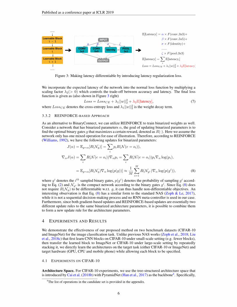
Figure 3: Making latency differentiable by introducing latency regularization loss.

We incorporate the expected latency of the network into the normal loss function by multiplying ascaling factor λ2(> 0) which controls the trade-off between accuracy and latency. The final lossfunction is given as (also shown in Figure 3 right)

Loss = LossCE + λ1||w||22 + λ2E[latency], (7)where LossCE denotes the cross-entropy loss and λ1||w||22 is the weight decay term.

3.3.2 REINFORCE-BASED APPROACH

As an alternative to BinaryConnect, we can utilize REINFORCE to train binarized weights as well.Consider a network that has binarized parameters α, the goal of updating binarized parameters is tofind the optimal binary gates g that maximizes a certain reward, denoted asR(·). Here we assume thenetwork only has one mixed operation for ease of illustration. Therefore, according to REINFORCE(Williams, 1992), we have the following updates for binarized parameters:

J(α) = Eg∼α[R(Ng)] =∑

i

piR(N (e = oi)),

∇αJ(α) =∑

i

R(N (e = oi))∇αpi =∑

i

R(N (e = oi))pi∇α log(pi),

= Eg∼α[R(Ng)∇α log(p(g))] ≈1

M

M∑

i=1

R(Ngi)∇α log(p(gi)), (8)

where gi denotes the ith sampled binary gates, p(gi) denotes the probability of sampling gi accord-ing to Eq. (2) and Ngi is the compact network according to the binary gates gi. Since Eq. (8) doesnot require R(Ng) to be differentiable w.r.t. g, it can thus handle non-differentiable objectives. Aninteresting observation is that Eq. (8) has a similar form to the standard NAS (Zoph & Le, 2017),while it is not a sequential decision-making process and no RNN meta-controller is used in our case.Furthermore, since both gradient-based updates and REINFORCE-based updates are essentially twodifferent update rules to the same binarized architecture parameters, it is possible to combine themto form a new update rule for the architecture parameters.

4 EXPERIMENTS AND RESULTS

We demonstrate the effectiveness of our proposed method on two benchmark datasets (CIFAR-10and ImageNet) for the image classification task. Unlike previous NAS works (Zoph et al., 2018; Liuet al., 2018c) that first learn CNN blocks on CIFAR-10 under small-scale setting (e.g. fewer blocks),then transfer the learned block to ImageNet or CIFAR-10 under large-scale setting by repeatedlystacking it, we directly learn the architectures on the target task (either CIFAR-10 or ImageNet) andtarget hardware (GPU, CPU and mobile phone) while allowing each block to be specified.

4.1 EXPERIMENTS ON CIFAR-10

Architecture Space. For CIFAR-10 experiments, we use the tree-structured architecture space thatis introduced by Cai et al. (2018b) with PyramidNet (Han et al., 2017) as the backbone4. Specifically,

4The list of operations in the candidate set is provided in the appendix.

6


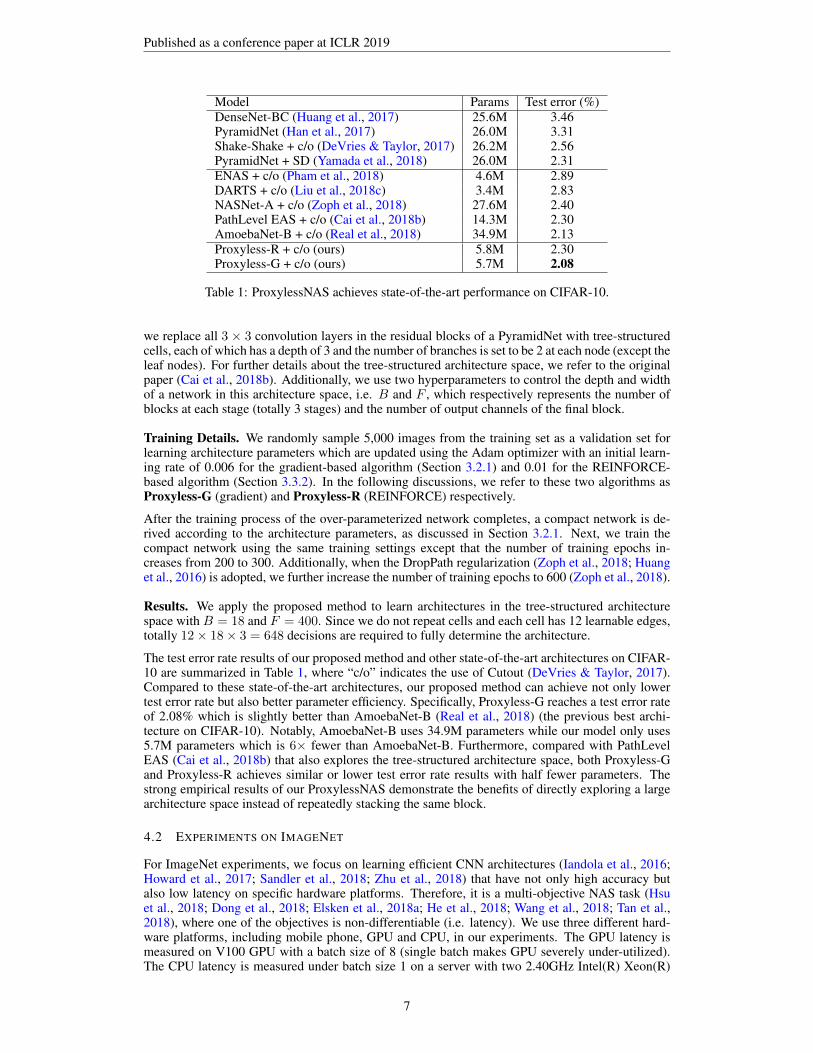
Model Params Test error (%)DenseNet-BC (Huang et al., 2017) 25.6M 3.46PyramidNet (Han et al., 2017) 26.0M 3.31Shake-Shake + c/o (DeVries & Taylor, 2017) 26.2M 2.56PyramidNet + SD (Yamada et al., 2018) 26.0M 2.31ENAS + c/o (Pham et al., 2018) 4.6M 2.89DARTS + c/o (Liu et al., 2018c) 3.4M 2.83NASNet-A + c/o (Zoph et al., 2018) 27.6M 2.40PathLevel EAS + c/o (Cai et al., 2018b) 14.3M 2.30AmoebaNet-B + c/o (Real et al., 2018) 34.9M 2.13Proxyless-R + c/o (ours) 5.8M 2.30Proxyless-G + c/o (ours) 5.7M 2.08

Table 1: ProxylessNAS achieves state-of-the-art performance on CIFAR-10.

we replace all 3 × 3 convolution layers in the residual blocks of a PyramidNet with tree-structuredcells, each of which has a depth of 3 and the number of branches is set to be 2 at each node (except theleaf nodes). For further details about the tree-structured architecture space, we refer to the originalpaper (Cai et al., 2018b). Additionally, we use two hyperparameters to control the depth and widthof a network in this architecture space, i.e. B and F , which respectively represents the number ofblocks at each stage (totally 3 stages) and the number of output channels of the final block.

Training Details. We randomly sample 5,000 images from the training set as a validation set forlearning architecture parameters which are updated using the Adam optimizer with an initial learn-ing rate of 0.006 for the gradient-based algorithm (Section 3.2.1) and 0.01 for the REINFORCE-based algorithm (Section 3.3.2). In the following discussions, we refer to these two algorithms asProxyless-G (gradient) and Proxyless-R (REINFORCE) respectively.

After the training process of the over-parameterized network completes, a compact network is de-rived according to the architecture parameters, as discussed in Section 3.2.1. Next, we train thecompact network using the same training settings except that the number of training epochs in-creases from 200 to 300. Additionally, when the DropPath regularization (Zoph et al., 2018; Huanget al., 2016) is adopted, we further increase the number of training epochs to 600 (Zoph et al., 2018).

Results. We apply the proposed method to learn architectures in the tree-structured architecturespace with B = 18 and F = 400. Since we do not repeat cells and each cell has 12 learnable edges,totally 12× 18× 3 = 648 decisions are required to fully determine the architecture.

The test error rate results of our proposed method and other state-of-the-art architectures on CIFAR-10 are summarized in Table 1, where “c/o” indicates the use of Cutout (DeVries & Taylor, 2017).Compared to these state-of-the-art architectures, our proposed method can achieve not only lowertest error rate but also better parameter efficiency. Specifically, Proxyless-G reaches a test error rateof 2.08% which is slightly better than AmoebaNet-B (Real et al., 2018) (the previous best archi-tecture on CIFAR-10). Notably, AmoebaNet-B uses 34.9M parameters while our model only uses5.7M parameters which is 6× fewer than AmoebaNet-B. Furthermore, compared with PathLevelEAS (Cai et al., 2018b) that also explores the tree-structured architecture space, both Proxyless-Gand Proxyless-R achieves similar or lower test error rate results with half fewer parameters. Thestrong empirical results of our ProxylessNAS demonstrate the benefits of directly exploring a largearchitecture space instead of repeatedly stacking the same block.

4.2 EXPERIMENTS ON IMAGENET

For ImageNet experiments, we focus on learning efficient CNN architectures (Iandola et al., 2016;Howard et al., 2017; Sandler et al., 2018; Zhu et al., 2018) that have not only high accuracy butalso low latency on specific hardware platforms. Therefore, it is a multi-objective NAS task (Hsuet al., 2018; Dong et al., 2018; Elsken et al., 2018a; He et al., 2018; Wang et al., 2018; Tan et al.,2018), where one of the objectives is non-differentiable (i.e. latency). We use three different hard-ware platforms, including mobile phone, GPU and CPU, in our experiments. The GPU latency ismeasured on V100 GPU with a batch size of 8 (single batch makes GPU severely under-utilized).The CPU latency is measured under batch size 1 on a server with two 2.40GHz Intel(R) Xeon(R)

7


Model Top-1 Top-5 Mobile Hardware No No Search costLatency -aware Proxy Repeat (GPU hours)

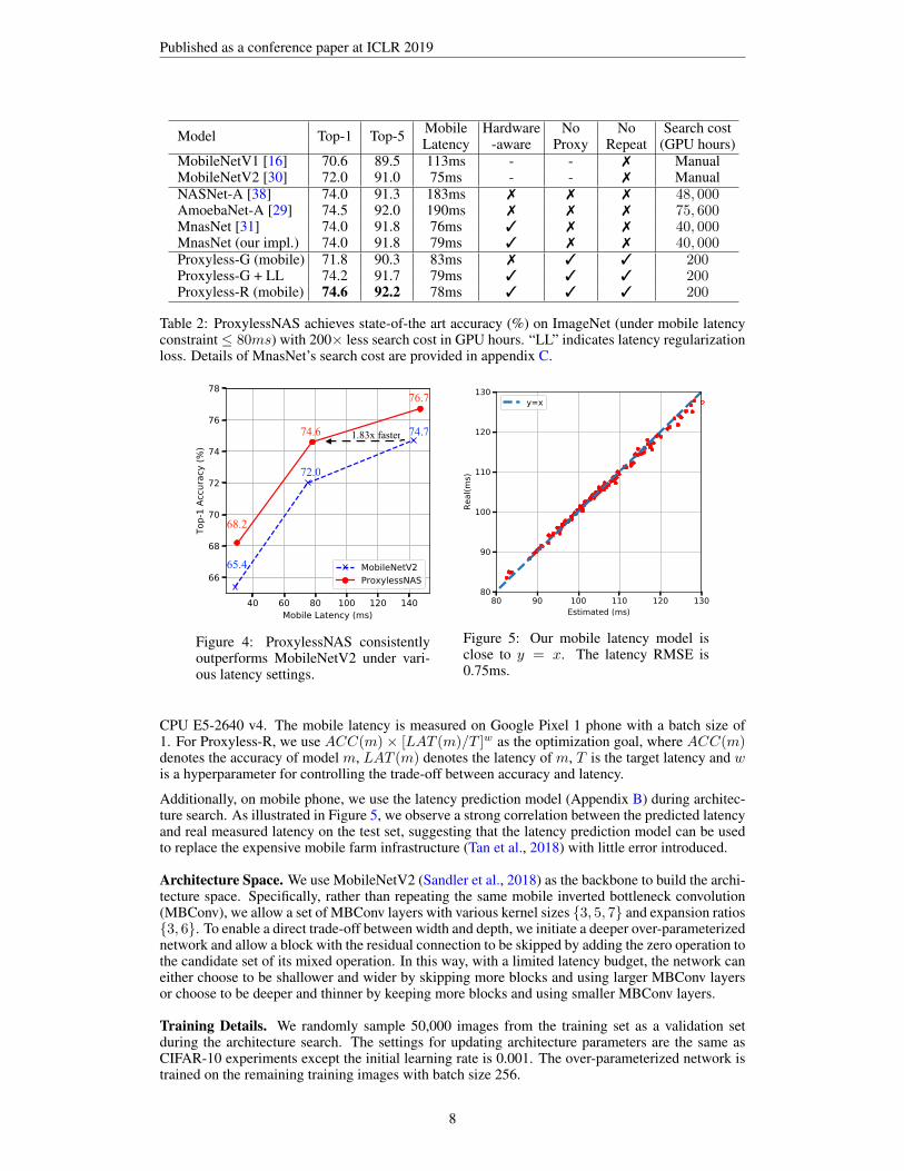
MobileNetV1 [16] 70.6 89.5 113ms - - 7 ManualMobileNetV2 [30] 72.0 91.0 75ms - - 7 ManualNASNet-A [38] 74.0 91.3 183ms 7 7 7 48, 000AmoebaNet-A [29] 74.5 92.0 190ms 7 7 7 75, 600MnasNet [31] 74.0 91.8 76ms 3 7 7 40, 000MnasNet (our impl.) 74.0 91.8 79ms 3 7 7 40, 000Proxyless-G (mobile) 71.8 90.3 83ms 7 3 3 200Proxyless-G + LL 74.2 91.7 79ms 3 3 3 200Proxyless-R (mobile) 74.6 92.2 78ms 3 3 3 200

Table 2: ProxylessNAS achieves state-of-the art accuracy (%) on ImageNet (under mobile latencyconstraint ≤ 80ms) with 200× less search cost in GPU hours. “LL” indicates latency regularizationloss. Details of MnasNet’s search cost are provided in appendix C.

74.6

76.7

68.2

65.4

72.0

74.71.83x faster

Figure 4: ProxylessNAS consistentlyoutperforms MobileNetV2 under vari-ous latency settings.

80 90 100 110 120 130Estimated (ms)

80

90

100

110

120

130

Real

(ms)

y=x

Figure 5: Our mobile latency model isclose to y = x. The latency RMSE is0.75ms.

CPU E5-2640 v4. The mobile latency is measured on Google Pixel 1 phone with a batch size of1. For Proxyless-R, we use ACC(m) × [LAT (m)/T ]w as the optimization goal, where ACC(m)denotes the accuracy of model m, LAT (m) denotes the latency of m, T is the target latency and wis a hyperparameter for controlling the trade-off between accuracy and latency.

Additionally, on mobile phone, we use the latency prediction model (Appendix B) during architec-ture search. As illustrated in Figure 5, we observe a strong correlation between the predicted latencyand real measured latency on the test set, suggesting that the latency prediction model can be usedto replace the expensive mobile farm infrastructure (Tan et al., 2018) with little error introduced.

Architecture Space. We use MobileNetV2 (Sandler et al., 2018) as the backbone to build the archi-tecture space. Specifically, rather than repeating the same mobile inverted bottleneck convolution(MBConv), we allow a set of MBConv layers with various kernel sizes {3, 5, 7} and expansion ratios{3, 6}. To enable a direct trade-off between width and depth, we initiate a deeper over-parameterizednetwork and allow a block with the residual connection to be skipped by adding the zero operation tothe candidate set of its mixed operation. In this way, with a limited latency budget, the network caneither choose to be shallower and wider by skipping more blocks and using larger MBConv layersor choose to be deeper and thinner by keeping more blocks and using smaller MBConv layers.

Training Details. We randomly sample 50,000 images from the training set as a validation setduring the architecture search. The settings for updating architecture parameters are the same asCIFAR-10 experiments except the initial learning rate is 0.001. The over-parameterized network istrained on the remaining training images with batch size 256.

8


Model Top-1 Top-5 GPU latencyMobileNetV2 (Sandler et al., 2018) 72.0 91.0 6.1msShuffleNetV2 (1.5) (Ma et al., 2018) 72.6 - 7.3msResNet-34 (He et al., 2016) 73.3 91.4 8.0msNASNet-A (Zoph et al., 2018) 74.0 91.3 38.3msDARTS (Liu et al., 2018c) 73.1 91.0 -MnasNet (Tan et al., 2018) 74.0 91.8 6.1msProxyless (GPU) 75.1 92.5 5.1ms

Table 3: ImageNet Accuracy (%) and GPU latency (Tesla V100) on ImageNet.

ImageNet Classification Results. We first apply our ProxylessNAS to learn specialized CNNmodels on the mobile phone. The summarized results are reported in Table 2. Compared to Mo-bileNetV2, our model improves the top-1 accuracy by 2.6% while maintaining a similar latency onthe mobile phone. Furthermore, by rescaling the width of the networks using a multiplier (San-dler et al., 2018; Tan et al., 2018), it is shown in Figure 4 that our model consistently outperformsMobileNetV2 by a significant margin under all latency settings. Specifically, to achieve the samelevel of top-1 accuracy performance (i.e. around 74.6%), MobileNetV2 has 143ms latency whileour model only needs 78ms (1.83× faster). While compared with MnasNet (Tan et al., 2018), ourmodel can achieve 0.6% higher top-1 accuracy with slightly lower mobile latency. More importantly,we are much more resource efficient: the GPU-hour is 200× fewer than MnasNet (Table 2).

Additionally, we also observe that Proxyless-G has no incentive to choose computation-cheap op-erations if were not for the latency regularization loss. Its resulting architecture initially has 158mslatency on Pixel 1. After rescaling the network using the multiplier, its latency reduces to 83ms.However, this model can only achieve 71.8% top-1 accuracy on ImageNet, which is 2.4% lowerthan the result given by Proxyless-G with latency regularization loss. Therefore, we conclude that itis essential to take latency as a direct objective when learning efficient neural networks.

Besides the mobile phone, we also apply our ProxylessNAS to learn specialized CNN models onGPU and CPU. Table 3 reports the results on GPU, where we find that our ProxylessNAS canstill achieve superior performances compared to both human-designed and automatically searchedarchitectures. Specifically, compared to MobileNetV2 and MnasNet, our model improves the top-1accuracy by 3.1% and 1.1% respectively while being 1.2× faster. Table 4 shows the summarizedresults of our searched models on three different platforms. An interesting observation is that modelsoptimized for GPU do not run fast on CPU and mobile phone, vice versa. Therefore, it is essential tolearn specialized neural networks for different hardware architectures to achieve the best efficiencyon different hardware.

Specialized Models for Different Hardware. Figure 6 demonstrates the detailed architectures ofour searched CNN models on three hardware platforms: GPU/CPU/Mobile. We notice that the ar-chitecture shows different preferences when targeting different platforms: (i) The GPU model isshallower and wider, especially in early stages where the feature map has higher resolution; (ii) TheGPU model prefers large MBConv operations (e.g. 7 × 7 MBConv6), while the CPU model wouldgo for smaller MBConv operations. This is because GPU has much higher parallelism than CPUso it can take advantage of large MBConv operations. Another interesting observation is that oursearched models on all platforms prefer larger MBConv operations in the first block within eachstage where the feature map is downsampled. We suppose it might because larger MBConv oper-ations are beneficial for the network to preserve more information when downsampling. Notably,such kind of patterns cannot be captured in previous NAS methods as they force the blocks to sharethe same structure (Zoph et al., 2018; Liu et al., 2018a).

5 CONCLUSION

We introduced ProxylessNAS that can directly learn neural network architectures on the target taskand target hardware without any proxy. We also reduced the search cost (GPU-hours and GPUmemory) of NAS to the same level of normal training using path binarization. Benefiting fromthe direct search, we achieve strong empirical results on CIFAR-10 and ImageNet. Furthermore,

9


April May June July

Region 1 Region 2

MB

1 3x

3

MB

3 5x

5

MB

3 7x

7

MB

6 7x

7

MB

3 5x

5

MB

6 5x

5

MB

3 3x

3

MB

3 5x

5

MB

6 7x

7

MB

6 7x

7

MB

6 7x

7

MB

6 5x

5

MB

6 7x

7

Con

v 3x

3

Poo

ling

FC

MB

3 3x

3 40x112x112

24x112x112

3x224x224

32x56x56

56x28x28

56x28x28

112x14x14

112x14x14

128x14x14

128x14x14

128x14x14

256x7x7

256x7x7

256x7x7

256x7x7

432x7x7

Con

v 3x

3

MB

1 3x

3

MB

3 5x

5

MB

3 3x

3

MB

3 7x

7

MB

3 3x

3

MB

3 5x

5

MB

3 5x

5

MB

6 7x

7 32x112x112

32x112x112

3x224x224

32x56x56

32x56x56

40x28x28

40x28x28

40x28x28

40x28x28

MB

3 5x

5

MB

3 5x

5

80x14x14

80x14x14

MB

6 5x

5

MB

3 5x

5

MB

3 5x

5

MB

3 5x

5

MB

6 7x

7

MB

3 7x

7

MB

6 7x

7

Poo

ling

FC

80x14x14

96x14x14

96x14x14

96x14x14

192x7x7

192x7x7

192x7x7

192x7x7

320x7x7

MB

3 5x

5

80x14x14

MB

6 7x

7

MB

3 7x

7

96x14x14

Con

v 3x

3

MB

1 3x

3

MB

6 3x

3

MB

3 3x

3

MB

3 3x

3

MB

3 3x

3

MB

6 3x

3

MB

3 3x

3

MB

3 3x

3 40x112x112

24x112x112

3x224x224

32x56x56

32x56x56

32x56x56

32x56x56

48x28x28

48x28x28

MB

6 3x

3

MB

3 5x

5

48x28x28

48x28x28

MB

6 5x

5

MB

3 3x

3

MB

3 3x

3

MB

3 3x

3

MB

6 5x

5

MB

3 3x

3

MB

6 5x

5

Poo

ling

FC

88x14x14

104x14x14

104x14x14

104x14x14

216x7x7

216x7x7

216x7x7

216x7x7

360x7x7

MB

3 3x

3

88x14x14

MB

3 5x

5

MB

3 5x

5

104x14x14

(1) Efficient mobile architecture found by ProxylessNAS.

(2) Efficient CPU architecture found by ProxylessNAS.

(3) Efficient GPU architecture found by ProxylessNAS.

MIT Red

(a) Efficient GPU model found by ProxylessNAS.

April May June July

Region 1 Region 2

MB

1 3x

3

MB

3 5x

5

MB

3 7x

7

MB

6 7x

7

MB

3 5x

5

MB

6 5x

5

MB

3 3x

3

MB

3 5x

5

MB

6 7x

7

MB

6 7x

7

MB

6 7x

7

MB

6 5x

5

MB

6 7x

7

Con

v 3x

3

Poo

ling

FC

MB

3 3x

3 40x112x112

24x112x112

3x224x224

32x56x56

56x28x28

56x28x28

112x14x14

112x14x14

128x14x14

128x14x14

128x14x14

256x7x7

256x7x7

256x7x7

256x7x7

432x7x7

Con

v 3x

3

MB

1 3x

3

MB

3 5x

5

MB

3 3x

3

MB

3 7x

7

MB

3 3x

3

MB

3 5x

5

MB

3 5x

5

MB

6 7x

7 32x112x112

32x112x112

3x224x224

32x56x56

32x56x56

40x28x28

40x28x28

40x28x28

40x28x28

MB

3 5x

5

MB

3 5x

5

80x14x14

80x14x14

MB

6 5x

5

MB

3 5x

5

MB

3 5x

5

MB

3 5x

5

MB

6 7x

7

MB

3 7x

7

MB

6 7x

7

Poo

ling

FC

80x14x14

96x14x14

96x14x14

96x14x14

192x7x7

192x7x7

192x7x7

192x7x7

320x7x7

MB

3 5x

5

80x14x14

MB

6 7x

7

MB

3 7x

7

96x14x14

Con

v 3x

3

MB

1 3x

3

MB

6 3x

3

MB

3 3x

3

MB

3 3x

3

MB

3 3x

3

MB

6 3x

3

MB

3 3x

3

MB

3 3x

3 40x112x112

24x112x112

3x224x224

32x56x56

32x56x56

32x56x56

32x56x56

48x28x28

48x28x28

MB

6 3x

3

MB

3 5x

5

48x28x28

48x28x28

MB

6 5x

5

MB

3 3x

3

MB

3 3x

3

MB

3 3x

3

MB

6 5x

5

MB

3 3x

3

MB

6 5x

5

Poo

ling

FC

88x14x14

104x14x14

104x14x14

104x14x14

216x7x7

216x7x7

216x7x7

216x7x7

360x7x7

MB

3 3x

3

88x14x14

MB

3 5x

5

MB

3 5x

5

104x14x14




MIT Red(b) Efficient CPU model found by ProxylessNAS.

April May June July

Region 1 Region 2

MB

1 3x

3

MB

3 5x

5

MB

3 7x

7

MB

6 7x

7

MB

3 5x

5

MB

6 5x

5

MB

3 3x

3

MB

3 5x

5

MB

6 7x

7

MB

6 7x

7

MB

6 7x

7

MB

6 5x

5

MB

6 7x

7

Con

v 3x

3

Poo

ling

FC

MB

3 3x

3 40x112x112

24x112x112

3x224x224

32x56x56

56x28x28

56x28x28

112x14x14

112x14x14

128x14x14

128x14x14

128x14x14

256x7x7

256x7x7

256x7x7

256x7x7

432x7x7

Con

v 3x

3

MB

1 3x

3

MB

3 5x

5

MB

3 3x

3

MB

3 7x

7

MB

3 3x

3

MB

3 5x

5

MB

3 5x

5

MB

6 7x

7 32x112x112

16x112x112

3x224x224

32x56x56

32x56x56

40x28x28

40x28x28

40x28x28

40x28x28

MB

3 5x

5

MB

3 5x

5

80x14x14

80x14x14

MB

6 5x

5

MB

3 5x

5

MB

3 5x

5

MB

3 5x

5

MB

6 7x

7

MB

3 7x

7

MB

6 7x

7

Poo

ling

FC

80x14x14

96x14x14

96x14x14

96x14x14

192x7x7

192x7x7

192x7x7

192x7x7

320x7x7

MB

3 5x

5

80x14x14

MB

6 7x

7

MB

3 7x

7

96x14x14

Con

v 3x

3

MB

1 3x

3

MB

6 3x

3

MB

3 3x

3

MB

3 3x

3

MB

3 3x

3

MB

6 3x

3

MB

3 3x

3

MB

3 3x

3 40x112x112

24x112x112

3x224x224

32x56x56

32x56x56

32x56x56

32x56x56

48x28x28

48x28x28

MB

6 3x

3

MB

3 5x

5

48x28x28

48x28x28

MB

6 5x

5

MB

3 3x

3

MB

3 3x

3

MB

3 3x

3

MB

6 5x

5

MB

3 3x

3

MB

6 5x

5

Poo

ling

FC

88x14x14

104x14x14

104x14x14

104x14x14

216x7x7

216x7x7

216x7x7

216x7x7

360x7x7

MB

3 3x

3

88x14x14

MB

3 5x

5

MB

3 5x

5

104x14x14




MIT Red

(c) Efficient mobile model found by ProxylessNAS.

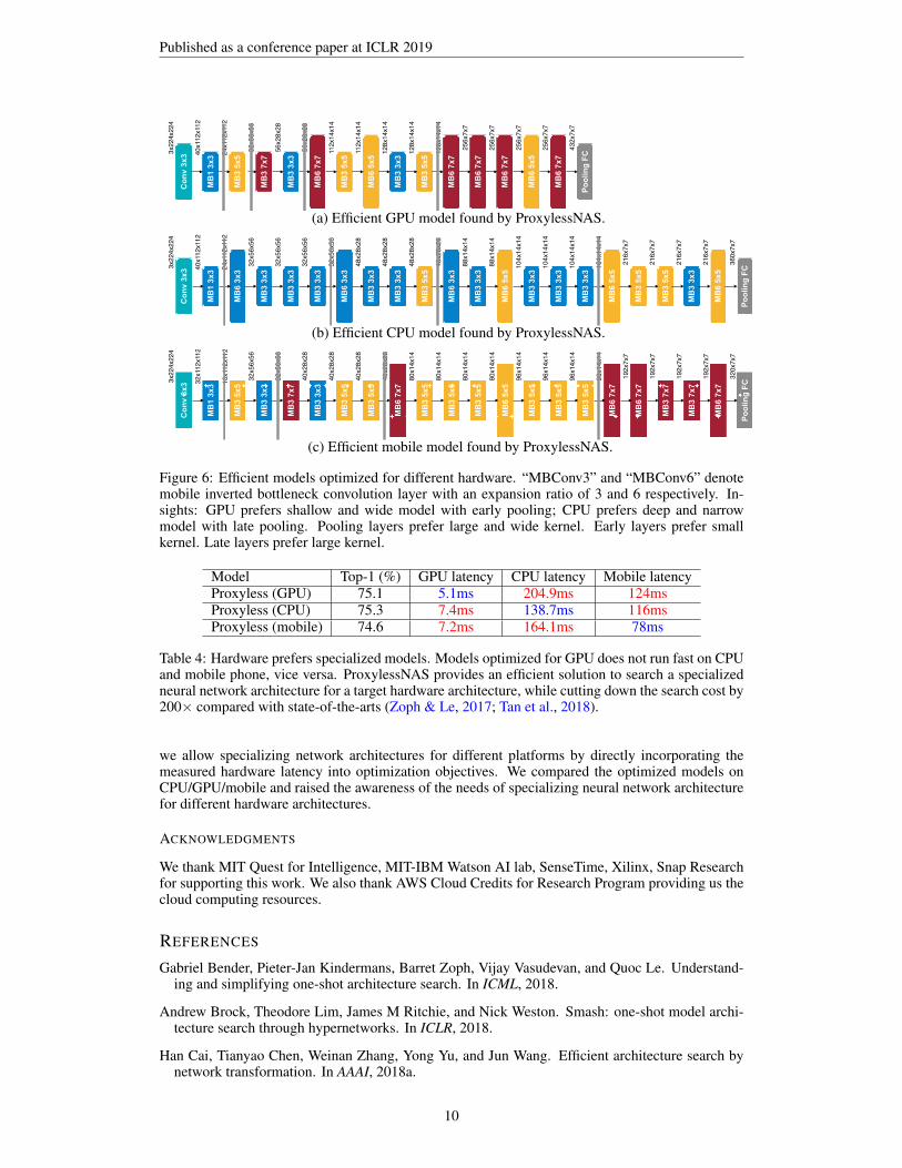
Figure 6: Efficient models optimized for different hardware. “MBConv3” and “MBConv6” denotemobile inverted bottleneck convolution layer with an expansion ratio of 3 and 6 respectively. In-sights: GPU prefers shallow and wide model with early pooling; CPU prefers deep and narrowmodel with late pooling. Pooling layers prefer large and wide kernel. Early layers prefer smallkernel. Late layers prefer large kernel.

Model Top-1 (%) GPU latency CPU latency Mobile latencyProxyless (GPU) 75.1 5.1ms 204.9ms 124msProxyless (CPU) 75.3 7.4ms 138.7ms 116msProxyless (mobile) 74.6 7.2ms 164.1ms 78ms

Table 4: Hardware prefers specialized models. Models optimized for GPU does not run fast on CPUand mobile phone, vice versa. ProxylessNAS provides an efficient solution to search a specializedneural network architecture for a target hardware architecture, while cutting down the search cost by200× compared with state-of-the-arts (Zoph & Le, 2017; Tan et al., 2018).

we allow specializing network architectures for different platforms by directly incorporating themeasured hardware latency into optimization objectives. We compared the optimized models onCPU/GPU/mobile and raised the awareness of the needs of specializing neural network architecturefor different hardware architectures.

ACKNOWLEDGMENTS

We thank MIT Quest for Intelligence, MIT-IBM Watson AI lab, SenseTime, Xilinx, Snap Researchfor supporting this work. We also thank AWS Cloud Credits for Research Program providing us thecloud computing resources.

REFERENCES

Gabriel Bender, Pieter-Jan Kindermans, Barret Zoph, Vijay Vasudevan, and Quoc Le. Understand-ing and simplifying one-shot architecture search. In ICML, 2018.

Andrew Brock, Theodore Lim, James M Ritchie, and Nick Weston. Smash: one-shot model archi-tecture search through hypernetworks. In ICLR, 2018.

Han Cai, Tianyao Chen, Weinan Zhang, Yong Yu, and Jun Wang. Efficient architecture search bynetwork transformation. In AAAI, 2018a.

10


Han Cai, Jiacheng Yang, Weinan Zhang, Song Han, and Yong Yu. Path-level network transformationfor efficient architecture search. In ICML, 2018b.

Matthieu Courbariaux, Yoshua Bengio, and Jean-Pierre David. Binaryconnect: Training deep neuralnetworks with binary weights during propagations. In NIPS, 2015.

Terrance DeVries and Graham W Taylor. Improved regularization of convolutional neural networkswith cutout. arXiv preprint arXiv:1708.04552, 2017.

Jin-Dong Dong, An-Chieh Cheng, Da-Cheng Juan, Wei Wei, and Min Sun. Dpp-net: Device-awareprogressive search for pareto-optimal neural architectures. In ECCV, 2018.

Thomas Elsken, Jan-Hendrik Metzen, and Frank Hutter. Simple and efficient architecture search forconvolutional neural networks. arXiv preprint arXiv:1711.04528, 2017.

Thomas Elsken, Jan Hendrik Metzen, and Frank Hutter. Multi-objective architecture search forcnns. arXiv preprint arXiv:1804.09081, 2018a.

Thomas Elsken, Jan Hendrik Metzen, and Frank Hutter. Neural architecture search: A survey. arXivpreprint arXiv:1808.05377, 2018b.

Dongyoon Han, Jiwhan Kim, and Junmo Kim. Deep pyramidal residual networks. In CVPR, 2017.

Song Han, Jeff Pool, John Tran, and William Dally. Learning both weights and connections forefficient neural network. In NIPS, 2015.

Song Han, Huizi Mao, and William J Dally. Deep compression: Compressing deep neural networkswith pruning, trained quantization and huffman coding. In ICLR, 2016.

Kaiming He, Xiangyu Zhang, Shaoqing Ren, and Jian Sun. Deep residual learning for image recog-nition. In CVPR, 2016.

Yihui He, Ji Lin, Zhijian Liu, Hanrui Wang, Li-Jia Li, and Song Han. Amc: Automl for modelcompression and acceleration on mobile devices. In ECCV, 2018.

Andrew G Howard, Menglong Zhu, Bo Chen, Dmitry Kalenichenko, Weijun Wang, Tobias Weyand,Marco Andreetto, and Hartwig Adam. Mobilenets: Efficient convolutional neural networks formobile vision applications. arXiv preprint arXiv:1704.04861, 2017.

Chi-Hung Hsu, Shu-Huan Chang, Da-Cheng Juan, Jia-Yu Pan, Yu-Ting Chen, Wei Wei, and Shih-Chieh Chang. Monas: Multi-objective neural architecture search using reinforcement learning.arXiv preprint arXiv:1806.10332, 2018.

Gao Huang, Yu Sun, Zhuang Liu, Daniel Sedra, and Kilian Q Weinberger. Deep networks withstochastic depth. In ECCV, 2016.

Gao Huang, Zhuang Liu, Laurens Van Der Maaten, and Kilian Q Weinberger. Densely connectedconvolutional networks. In CVPR, 2017.

Forrest N Iandola, Song Han, Matthew W Moskewicz, Khalid Ashraf, William J Dally, and KurtKeutzer. Squeezenet: Alexnet-level accuracy with 50x fewer parameters and¡ 0.5 mb model size.arXiv preprint arXiv:1602.07360, 2016.

Purushotham Kamath, Abhishek Singh, and Debo Dutta. Neural architecture construction usingenvelopenets. arXiv preprint arXiv:1803.06744, 2018.

Chenxi Liu, Barret Zoph, Jonathon Shlens, Wei Hua, Li-Jia Li, Li Fei-Fei, Alan Yuille, JonathanHuang, and Kevin Murphy. Progressive neural architecture search. In ECCV, 2018a.

Hanxiao Liu, Karen Simonyan, Oriol Vinyals, Chrisantha Fernando, and Koray Kavukcuoglu. Hi-erarchical representations for efficient architecture search. In ICLR, 2018b.

Hanxiao Liu, Karen Simonyan, and Yiming Yang. Darts: Differentiable architecture search. arXivpreprint arXiv:1806.09055, 2018c.

11


Zhuang Liu, Jianguo Li, Zhiqiang Shen, Gao Huang, Shoumeng Yan, and Changshui Zhang. Learn-ing efficient convolutional networks through network slimming. In ICCV, 2017.

Renqian Luo, Fei Tian, Tao Qin, and Tie-Yan Liu. Neural architecture optimization. arXiv preprintarXiv:1808.07233, 2018.

Ningning Ma, Xiangyu Zhang, Hai-Tao Zheng, and Jian Sun. Shufflenet v2: Practical guidelines forefficient cnn architecture design. In ECCV, 2018.

Hieu Pham, Melody Y Guan, Barret Zoph, Quoc V Le, and Jeff Dean. Efficient neural architecturesearch via parameter sharing. In ICML, 2018.

Esteban Real, Alok Aggarwal, Yanping Huang, and Quoc V Le. Regularized evolution for imageclassifier architecture search. arXiv preprint arXiv:1802.01548, 2018.

Mark Sandler, Andrew Howard, Menglong Zhu, Andrey Zhmoginov, and Liang-Chieh Chen. Mo-bilenetv2: Inverted residuals and linear bottlenecks. In CVPR, 2018.

Mingxing Tan, Bo Chen, Ruoming Pang, Vijay Vasudevan, and Quoc V Le. Mnasnet: Platform-aware neural architecture search for mobile. arXiv preprint arXiv:1807.11626, 2018.

Kuan Wang, Zhijian Liu, Yujun Lin, Ji Lin, and Song Han. Haq: Hardware-aware automated quan-tization. arXiv, 2018.

Ronald J Williams. Simple statistical gradient-following algorithms for connectionist reinforcementlearning. In Reinforcement Learning. 1992.

Yoshihiro Yamada, Masakazu Iwamura, and Koichi Kise. Shakedrop regularization. arXiv preprintarXiv:1802.02375, 2018.

Zhao Zhong, Junjie Yan, Wei Wu, Jing Shao, and Cheng-Lin Liu. Practical block-wise neuralnetwork architecture generation. In CVPR, 2018.

Ligeng Zhu, Ruizhi Deng, Michael Maire, Zhiwei Deng, Greg Mori, and Ping Tan. Sparsely aggre-gated convolutional networks. In Proceedings of the European Conference on Computer Vision(ECCV), pp. 186–201, 2018.

Barret Zoph and Quoc V Le. Neural architecture search with reinforcement learning. In ICLR, 2017.

Barret Zoph, Vijay Vasudevan, Jonathon Shlens, and Quoc V Le. Learning transferable architecturesfor scalable image recognition. In CVPR, 2018.

12


A THE LIST OF CANDIDATE OPERATIONS USED ON CIFAR-10

We adopt the following 7 operations in our CIFAR-10 experiments:

• 3× 3 dilated depthwise-separable convolution• Identity• 3× 3 depthwise-separable convolution• 5× 5 depthwise-separable convolution• 7× 7 depthwise-separable convolution• 3× 3 average pooling• 3× 3 max pooling

B MOBILE LATENCY PREDICTION

Measuring the latency on-device is accurate but not ideal for scalable neural architecture search.There are two reasons: (i) Slow. As suggested in TensorFlow-Lite, we need to average hundredsof runs to produce a precise measurement, approximately 20 seconds. This is far more slowerthan a single forward / backward execution. (ii) Expensive. A lot of mobile devices and softwareengineering work are required to build an automatic pipeline to gather the latency from a mobilefarm. Instead of direct measurement, we build a model to estimate the latency. We need only 1phone rather than a farm of phones, which has only 0.75ms latency RMSE. We use the latencymodel to search, and we use the measured latency to report the final model’s latency.

We sampled 5k architectures from our candidate space, where 4k architectures are used to build thelatency model and the rest are used for test. We measured the latency on Google Pixel 1 phone usingTensorFlow-Lite. The features include (i) type of the operator (ii) input and output feature map size(iii) other attributes like kernel size, stride for convolution and expansion ratio.

C DETAILS OF MNASNET’S SEARCH COST

Mnas (Tan et al., 2018) trains 8,000 mobile-sized models on ImageNet, each of which is trainedfor 5 epochs for learning architectures. If these models are trained on V100 GPUs, as done in ourexperiments, the search cost is roughly 40,000 GPU hours.

D IMPLEMENTAION OF THE GRADIENT-BASED ALGORITHM

A naive implementation of the gradient-based algorithm (see Eq. (4)) is calculating and storing oj(x)in the forward step to later compute ∂L/∂gj in the backward step:

∂L/∂gj = reduce sum(∇yL ◦ oj(x)), (9)

where∇yL denotes the gradient w.r.t. the output of the mixed operation y, “◦” denotes the element-wise product, and “reduce sum(·)” denotes the sum of all elements.

Notice that oj(x) is only used for calculating ∂L/∂gj when jth path is not active (i.e. not involvedin calculating y). So we do not need to actually allocate GPU memory to store oj(x). Instead, wecan calculate oj(x) after getting∇yL in the backward step, use oj(x) to compute ∂L/∂gj followingEq. (9), then release the occupied GPU memory. In this way, without the approximation discussedin Section 3.2.1, we can reduce the GPU memory cost to the same level of training a compact model.

13

p nas: direct neural architecture s task and hardware

Documents