p p u p t m s p u t m l o a z - gulf coast...

P P U P T M S P U T

M L O A

Hunter Berch1 and Jeffrey Nunn2 1Department of Geology and Geophysics, Louisiana State University,

E235 Howe-Russell Bldg., Baton Rouge, Louisiana 70803, U.S.A. Present address: Chevron Exploration and Production,

100 Northpark Blvd., Covington, Louisiana 70433, U.S.A. 2Department of Geology and Geophysics, Louisiana State University,

E235 Howe-Russell Bldg., Baton Rouge, Louisiana 70803, U.S.A. Present address: Chevron Energy Technology Company,

1500 Louisiana St., Houston, Texas 77002, U.S.A.

ABSTRACT The Tuscaloosa Marine Shale formation (TMS) of central Louisiana and southern Mississippi was suggested as a potential

hydrocarbon play with up to seven billion barrels of reserves in a 1997 study by Louisiana State University’s Basin Research Institute. The TMS is a Upper Cretaceous gray to black fissile marine shale and occurs at depths between 10,000 and 19,000 ft in the study area. Since 1997, horizontal drilling and hydraulic fracturing have enabled exploration and documentation of oil reserves in this play. In this study, information from sonic logs and resistivity logs from 43 wells were used to estimate thermal maturation. Model results indicate that TMS is in the oil to condensate–wet gas zones with vitrinite reflectance (%Ro) ranging from 0.6 to 1.2%Ro. Total organic carbon (TOC) was estimated using an overlay technique for sonic and resistivity logs. Esti-mated TOC in the study area ranges from 0.5 to 3% and has a complex spatial distribution. TOC results were calibrated using core and cuttings data provided by operators active in the TMS. This research has provided a technique to predict areas with higher concentrations of TOC that are thermally mature, which are commonly associated with areas of unconventional produc-tion potential.

69

INTRODUCTION Unconventional hydrocarbons are produced from geologic

media, such as shales or mudrocks that were thought to lack the porosity and permeability necessary to produce hydrocarbons (International Energy Agency, 2012). Whereas shale plays lack the permeability necessary to produce hydrocarbons, they do have sufficient porosity necessary to hold economic amounts of gases and liquids. The Tuscaloosa Marine Shale (TMS) of cen-tral Louisiana and southern Mississippi (Fig. 1) is considered a potentially prolific shale play because of its: (1) thermal matura-tion, (2) large lateral extent and thickness, and (3) close geo-

graphic and stratigraphic proximity to the notable Eagle Ford Shale play (John et al, 1997). Since 1997, multiple vertical and horizontal wells have been completed in the TMS. Horizontally drilled wells with completions involving multiple fracture stages have unconventionally produced economical amounts of hydro-carbons in the central portion of the play (Barrell, 2011).

In this study, publicly available well logs were used to deter-mine burial depth, lithology, and relative age of stratigraphy down to the TMS interval. This information is transferred to Schlumberger’s PetroMod® thermal modeling software, which calculates temperature and vitrinite reflectance (%Ro). %Ro indicates the thermal maturity of the TMS, thus specifying whether or not kerogen has been converted into oil and/or gas. %Ro is then converted to level of organic metamorphism (LOM) by inverting an equation developed by Lecompte and Hursan (2010). LOM values, resistivity logs, sonic logs, and correlation logs are then used to estimate total organic carbon (TOC) through log overlay analysis (Passey et al., 1990). The method used in this study effectively utilizes public data to identify thermally

Copyright © 2014. Gulf Coast Association of Geological Societies. All rights reserved. Manuscript received March 24, 2014; revised manuscript received July 3, 2014; manuscript accepted July 8, 2014. GCAGS Journal, v. 3 (2014), p. 69–78.

A Publication of the Gulf Coast Association of Geological Societies

www.gcags.org

70 Hunter Berch and Jeffrey Nunn

mature and organic-rich areas within the TMS play. This study was motivated by a group of operators who provided support for graduate student research to guide development of the TMS play.

The study area includes the following parishes in Louisiana: Vernon, Natchitoches, Rapides, Grant, Allen, Evangeline, Avoyelles, St. Landry, Point Coupee, West Feliciana, East Felici-ana, West Baton Rouge, East Baton Rouge, St. Helena, Living-ston, Tangipahoa, Washington, and St. Tammany (Fig. 2). In addition, the study area includes the following counties in Missis-sippi: Wilkinson, Adams, Amite, Pike, and Walthall (Fig. 2).

GEOLOGIC SETTING

The study area is located within the Gulf of Mexico (GOM) Basin (Fig. 1). The GOM Basin lies on a passive continental margin that is characterized by extensional deformation and wrench faulting (Mancini et al., 2008). Formation of northern GOM was caused by Early Jurassic rifting which thinned the lithosphere, followed by thermal subsidence through the Early Cretaceous (Mancini et al., 2008). Positive features in the region are the Sabine Uplift (northwest of the study area), Monroe Up-lift (north of the study area), LaSalle Arch (north of the study area), and Wiggins Arch (northeast of the study area). Nunn et al. (1984) suggested that the Sabine and Monroe uplifts are com-posed of continental lithosphere that experienced little to no ex-tensional deformation during the opening of the GOM, and Law-less and Hart (1990) concluded that the less prominent LaSalle Arch is also underlain by the same continental lithosphere. The LaSalle and Wiggins Arches have higher present day heat flow (SMU, 2011) presumably due to higher radiogenic heat produc-tion in the thicker crust.

The Tuscaloosa Group is composed of upper, middle, and lower units (John et al., 1997) (Fig. 3). The youngest sediments in the Tuscaloosa Group are Late Turonian in age, and the oldest sediments are Late Cenomanian. Sands and shales of the Tusca-loosa Group are approximately 1000 ft thick in the study area, and they are thought to represent a full depositional cycle (John et al., 1997). The lower Tuscaloosa represents the transgressive stage of the depositional cycle, and the upper Tuscaloosa repre-sents the regressive stage. In the study area, the Middle Tusca-

loosa is composed almost entirely of a grey to black, fissile, and sometimes sandy marine shale which thickens down-dip (John et al., 1997). This unit is commonly called the “Tuscaloosa Marine Shale,” and it represents the inundated stage of the depositional cycle, otherwise known as the transgressive systems tract.

DATA AND METHODS

Digital wireline and LWD logs from 43 wells with spontane-ous potential (SP) and resistivity (RES) curves were used in this study (Fig. 2, Appendix). Most well logs also contained gamma ray (GR) and sonic (DT) curves as well. Vitrinite reflectance, Tmax, and TOC data measured from conventional cores, sidewall cores, and drill cuttings from 8 wells were used for calibration purposes in this study (Fig. 2; Table 1). Five of these wells also had mineralogy determined from XRD.

Mapping using GeoGraphix®

43 well surface locations were loaded into Landmark/Haliburton’s Geographix® software and gridded using geographic latitude and longitude in the World–Mercator coordinate system. The NAD83 Louisiana–High Accuracy Reference Network da-tum was used as the reference geographic reference point. Shape files for Louisiana and Mississippi state outlines and parishes/counties were downloaded from the Strategic Online Natural Resources Information System (SONRIS) website (www.sonris.com) and the Mississippi Automated Resource In-formation System (MARIS) website (www.maris.state.ms.us), respectively, and imported into Geographix®. Digital log files were imported into Geographix® as LAS files.

Formations were correlated in the Landmark/Haliburton’s Prizm® log analysis module based on their respective log re-sponses in the study area (Fig. 3). The Selma Chalk (equivalent to the Austin Chalk in Texas) formation has low GR values of ~30 API units and a blocky RES signature peaking around 80 ohm-m. The Upper Tuscaloosa member has a relatively high and flat GR signature with values around 75 API units and RES val-ues between 2 and 20 ohm-m. The TMS was correlated from the base to the top, and its only consistently distinguishable log char-

Figure 1. Geologic map showing structural features of Louisiana and Mississippi. TMS in green and paleo-shelf edge in blue (modified after Barrell, 2013).

71 Predicting Potential Unconventional Production in the Tuscaloosa Marine Shale Play

acteristic is its high resistivity (20 ohm-m) interval at its base, which immediately terminates into the lower resistivity Lower Tuscaloosa Massive Sand beneath it. Generally, everything with-in a 50–150 ft range above the Lower Tuscaloosa Massive Sand is considered the TMS interval. Above the TMS is the less or-ganic-rich Upper Tuscaloosa. GR and SP signatures are not con-sistent across the TMS. Downsection, the Lower Tuscaloosa sands have low GR and RES values (refer to Fig. 3 for log signa-tures).

Maturation Calculations using PetroMod®

1–D numerical models were created using Schlumberger’s PetroMod® 2011 software in order to calculate subsidence, tem-perature, and %Ro as a function of time for 43 wells in the study area. Input information required to construct 1–D models in PetroMod® included thickness, deposition ages, and lithology for each distinguishable formation used in the model (Figs. 4–5). Lithology and approximate ages in million years ago (Ma) for each layer were adapted from Mancini et al. (2008). %Ro values are estimated using the EASY %Ro algorithm (Sweeney and

Burham, 1990) which is the default for PetroMod® 2011 soft-ware. Implications of using a different kinetic model for estimat-ing %Ro from temperature history are presented in the discussion section.

Basal heat flow, water depth, and surface temperature versus time are required to complete a thermal history model using PetroMod®. Paleo-heatflow is derived using the McKenzie mod-el (McKenzie, 1978). The model is based on an initial period of uniform extension of the lithosphere followed by a period of cooling associated with rejuvenation of the earlier thermal thick-ness of the lithosphere (Hantschel and Kauerauf, 2009). Rifting ages of 225 Ma to 160 Ma, and thermal subsidence ages of 160 Ma to 135 Ma were used in the McKenzie models. Beta factors between 1.8 and 2.3 were used in model calculations based on geographic location (Fig. 2). Models closest to the Sabine Uplift were given lower beta factors, while southerly models were given higher beta factors. Present day heat flow in model calculations is calibrated with the SMU (2011) heat flow map. Model heat flow is constant 41.5 million yr prior to TMS deposition, thus elevated heat flow associated with rifting and subsidence before TMS deposition does not affect the TMS thermal model.

Figure 2. Map of study area in Louisiana and Mississippi. Wells used in this study are shown as purple dots. Wells with geo-chemical data are circled in orange. Well names and locations given in the Appendix.

Well Core %Ro Model %Ro Core TOC Model

TOC Quartz (%) Calcite (%) Clay (%)

Ellis Estate 0.76–1.16 0.8 0.7–1.74 1.45 21–36 3–31 37–55 Deshotels 0.89–1.25 1.14 1.5–2.35 2.33 15–41 8–30 31–55 Bentley 32 0.94–1.26 1.04 0.12–2.13 1.21 25–64 0–39 1–60 Bentley 34 0.81–0.94 0.83 0.08–1.3 0.45 27–56 1–36 10–53 Spinks 0.67–0.81 0.7 0.41–1.36 2.0 25–45 8–39 30–45 Zap Minerals 0.74–0.98 0.78 0.64–1.19 0.83 N/A N/A N/A Richland 0.58–0.72 0.84 0.49–1.08 2.16 N/A N/A N/A Brian 0.17–0.72 1.34 0.09–0.44 1.34 N/A N/A N/A

Table 1. Geochemical and mineralogical data.

The oyster packstones and claystones of the TMS in South-west Alabama contain evidence of fauna that were typical of a Cretaceous open-marine shelf environment, so the TMS was most likely deposited on a shallow open-marine shelf (Mancini et al., 1987). A typical Cretaceous open-marine shelf in the GOM was estimated to have paleo-water depth (PWD) of 500 ft (Cardneaux, 2012). In PetroMod®, the sediment water interface temperature (SWIT) or water bottom temperature is the base temperature for the heat flow calculation (Hantschel and Kau-erauf, 2009). PetroMod® utilizes a SWIT model based on

Wygrala (1989) to get a mean air surface temperature, which is affected by latitude and global climate change throughout geo-logical history (Hantschel and Kauerauf, 2009). SWIT was cal-culated to be ~24°C during the time of TMS deposition, which is slightly lower than mean air surface temperature (27.5°C) be-cause of the presence of 500 ft water on the open-marine shelf. The study area was closer to the equator and mean global temper-atures were hotter during the Cretaceous.

PetroMod® software uses the above information to create a geohistory curve which is a simulation of subsidence and temper-

Figure 3. Stratigraphic column (modified after John et al., 1997) and type log from study area.

Figure 4. Temperature versus time computed by PetroMod® for the Deshotels 20H well (well 38 in Figure 2). Each black line represents the depth of a hori-zon top versus time. Colors are temperature: Blue (cold) to red (hot).


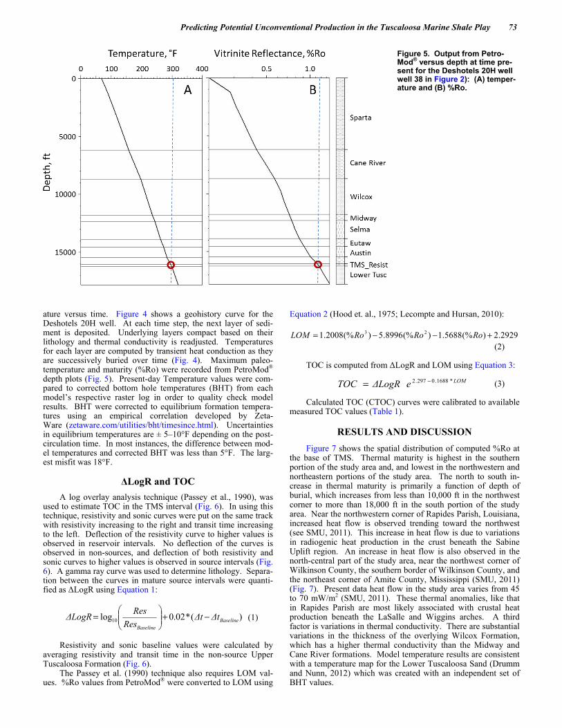
ature versus time. Figure 4 shows a geohistory curve for the Deshotels 20H well. At each time step, the next layer of sedi-ment is deposited. Underlying layers compact based on their lithology and thermal conductivity is readjusted. Temperatures for each layer are computed by transient heat conduction as they are successively buried over time (Fig. 4). Maximum paleo-temperature and maturity (%Ro) were recorded from PetroMod® depth plots (Fig. 5). Present-day Temperature values were com-pared to corrected bottom hole temperatures (BHT) from each model’s respective raster log in order to quality check model results. BHT were corrected to equilibrium formation tempera-tures using an empirical correlation developed by Zeta- Ware (zetaware.com/utilities/bht/timesince.html). Uncertainties in equilibrium temperatures are ± 5–10°F depending on the post-circulation time. In most instances, the difference between mod-el temperatures and corrected BHT was less than 5°F. The larg-est misfit was 18°F.

ΔLogR and TOC

A log overlay analysis technique (Passey et al., 1990), was used to estimate TOC in the TMS interval (Fig. 6). In using this technique, resistivity and sonic curves were put on the same track with resistivity increasing to the right and transit time increasing to the left. Deflection of the resistivity curve to higher values is observed in reservoir intervals. No deflection of the curves is observed in non-sources, and deflection of both resistivity and sonic curves to higher values is observed in source intervals (Fig. 6). A gamma ray curve was used to determine lithology. Separa-tion between the curves in mature source intervals were quanti-fied as ΔLogR using Equation 1:

(1) Resistivity and sonic baseline values were calculated by

averaging resistivity and transit time in the non-source Upper Tuscaloosa Formation (Fig. 6).

The Passey et al. (1990) technique also requires LOM val-ues. %Ro values from PetroMod® were converted to LOM using

Equation 2 (Hood et. al., 1975; Lecompte and Hursan, 2010):

(2) TOC is computed from ΔLogR and LOM using Equation 3:

(3) Calculated TOC (CTOC) curves were calibrated to available

measured TOC values (Table 1).

RESULTS AND DISCUSSION Figure 7 shows the spatial distribution of computed %Ro at

the base of TMS. Thermal maturity is highest in the southern portion of the study area and, and lowest in the northwestern and northeastern portions of the study area. The north to south in-crease in thermal maturity is primarily a function of depth of burial, which increases from less than 10,000 ft in the northwest corner to more than 18,000 ft in the south portion of the study area. Near the northwestern corner of Rapides Parish, Louisiana, increased heat flow is observed trending toward the northwest (see SMU, 2011). This increase in heat flow is due to variations in radiogenic heat production in the crust beneath the Sabine Uplift region. An increase in heat flow is also observed in the north-central part of the study area, near the northwest corner of Wilkinson County, the southern border of Wilkinson County, and the northeast corner of Amite County, Mississippi (SMU, 2011) (Fig. 7). Present data heat flow in the study area varies from 45 to 70 mW/m2 (SMU, 2011). These thermal anomalies, like that in Rapides Parish are most likely associated with crustal heat production beneath the LaSalle and Wiggins arches. A third factor is variations in thermal conductivity. There are substantial variations in the thickness of the overlying Wilcox Formation, which has a higher thermal conductivity than the Midway and Cane River formations. Model temperature results are consistent with a temperature map for the Lower Tuscaloosa Sand (Drumm and Nunn, 2012) which was created with an independent set of BHT values.

Figure 5. Output from Petro-Mod® versus depth at time pre-sent for the Deshotels 20H well well 38 in Figure 2): (A) temper-ature and (B) %Ro.

)(*02.0log10 BaselineBaseline

ΔtΔtRes

ResΔLogR −+

=

2929.2)(%5688.1)(%8996.5)(%2008.1 23 +−−= RoRoRoLOM

LOMe ΔLogRTOC *1688.0297.2 −=


http://www.zetaware.com/utilities/bht/timesince.html

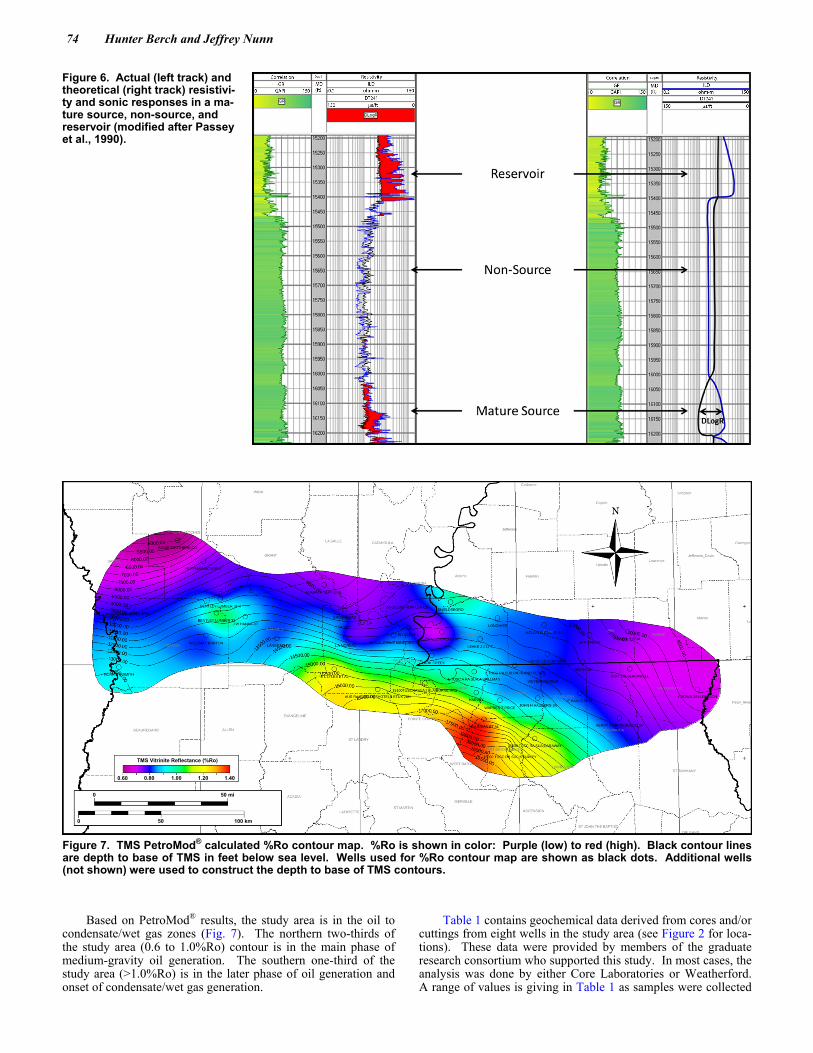
Based on PetroMod® results, the study area is in the oil to condensate/wet gas zones (Fig. 7). The northern two-thirds of the study area (0.6 to 1.0%Ro) contour is in the main phase of medium-gravity oil generation. The southern one-third of the study area (>1.0%Ro) is in the later phase of oil generation and onset of condensate/wet gas generation.

Table 1 contains geochemical data derived from cores and/or cuttings from eight wells in the study area (see Figure 2 for loca-tions). These data were provided by members of the graduate research consortium who supported this study. In most cases, the analysis was done by either Core Laboratories or Weatherford. A range of values is giving in Table 1 as samples were collected

Figure 6. Actual (left track) and theoretical (right track) resistivi-ty and sonic responses in a ma-ture source, non-source, and reservoir (modified after Passey et al., 1990).

Figure 7. TMS PetroMod® calculated %Ro contour map. %Ro is shown in color: Purple (low) to red (high). Black contour lines are depth to base of TMS in feet below sea level. Wells used for %Ro contour map are shown as black dots. Additional wells (not shown) were used to construct the depth to base of TMS contours.

0 50 mi

0 50 100 km

TMS Vitrinite Reflectance (%Ro)

0.60 0.80 1.00 1.20 1.40


across the entire TMS and in some cases above and/or below whereas model results are an average for the most resistive por-tion of the TMS which is in the middle of the TMS (Fig. 8). Thus, model results should fall between the maximum and mini-mum values of the core analyses.

The Ellis Estate well was the only instance where %Ro was directly measured. Values range from 0.76 and 1.16 and there was a bimodal distribution. The analysis concluded that the low-er mode was more representative of the thermal maturity and that higher values were due to oxidation of samples. Model results for the resistive TMS were 0.8. The other estimates of %Ro from core analysis comes from Tmax values from pyrolysis using an empirical formula derived by Jarvie et al. (2001) for the Barnett Shale (%Ro = 0.018 * Tmax – 7.16). For the Deshotels 20H, Bentley 32, Bentley 34, Spinks, and Zap Minerals wells, the model %Ro falls in between the core values. Usually it is closer to the minimum value. The model %Ro value for the Richland well is higher than the estimates from Tmax. The 3 samples used in the Richland analysis all had low S2 values which makes Tmax values unreliably low. Finally, the model %Ro value of 1.34 for the Brian well is dramatically higher than the values estimated from Tmax (<0.72). The TMS is at around 16,000 ft in the Brian well with a corrected BHT at that depth of 317°F, which is incompatible with a %Ro of 0.72 or less estimated from Tmax.

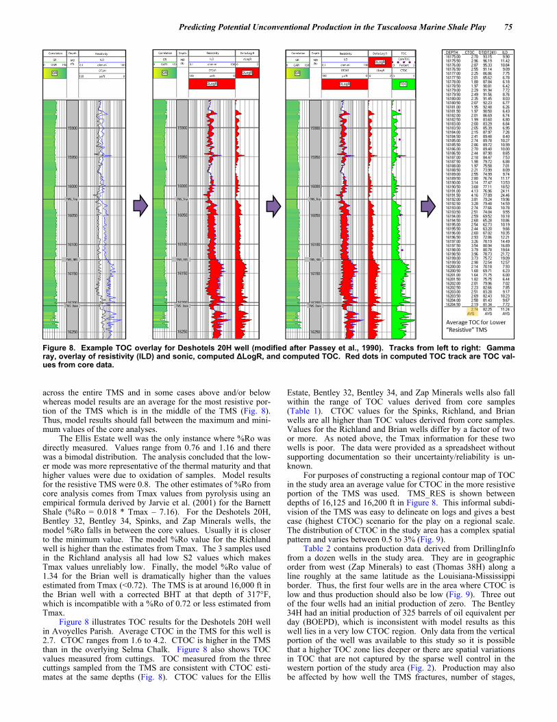
Figure 8 illustrates TOC results for the Deshotels 20H well in Avoyelles Parish. Average CTOC in the TMS for this well is 2.7. CTOC ranges from 1.6 to 4.2. CTOC is higher in the TMS than in the overlying Selma Chalk. Figure 8 also shows TOC values measured from cuttings. TOC measured from the three cuttings sampled from the TMS are consistent with CTOC esti-mates at the same depths (Fig. 8). CTOC values for the Ellis

Estate, Bentley 32, Bentley 34, and Zap Minerals wells also fall within the range of TOC values derived from core samples (Table 1). CTOC values for the Spinks, Richland, and Brian wells are all higher than TOC values derived from core samples. Values for the Richland and Brian wells differ by a factor of two or more. As noted above, the Tmax information for these two wells is poor. The data were provided as a spreadsheet without supporting documentation so their uncertainty/reliability is un-known.

For purposes of constructing a regional contour map of TOC in the study area an average value for CTOC in the more resistive portion of the TMS was used. TMS_RES is shown between depths of 16,125 and 16,200 ft in Figure 8. This informal subdi-vision of the TMS was easy to delineate on logs and gives a best case (highest CTOC) scenario for the play on a regional scale. The distribution of CTOC in the study area has a complex spatial pattern and varies between 0.5 to 3% (Fig. 9).

Table 2 contains production data derived from DrillingInfo from a dozen wells in the study area. They are in geographic order from west (Zap Minerals) to east (Thomas 38H) along a line roughly at the same latitude as the Louisiana-Mississippi border. Thus, the first four wells are in the area where CTOC is low and thus production should also be low (Fig. 9). Three out of the four wells had an initial production of zero. The Bentley 34H had an initial production of 325 barrels of oil equivalent per day (BOEPD), which is inconsistent with model results as this well lies in a very low CTOC region. Only data from the vertical portion of the well was available to this study so it is possible that a higher TOC zone lies deeper or there are spatial variations in TOC that are not captured by the sparse well control in the western portion of the study area (Fig. 2). Production may also be affected by how well the TMS fractures, number of stages,

Figure 8. Example TOC overlay for Deshotels 20H well (modified after Passey et al., 1990). Tracks from left to right: Gamma ray, overlay of resistivity (ILD) and sonic, computed ΔLogR, and computed TOC. Red dots in computed TOC track are TOC val-ues from core data.


and length of the lateral as well as TOC level. The remaining eight wells are in the high TOC area along the Louisiana-Mississippi border (Fig. 9). These wells all have initial produc-tion values between 192-1300 BOEPD. The highest levels of initial production are associated with estimated TOC of 2.5 or higher.

In this study, a simple kinetic model (Sweeney and Burn-ham, 1990) was used to compute %Ro for the TMS. This model does not distinguish between different types of kerogen and uses a single kinetic reaction equation. A more accurate kinetic model would have included information on kerogen type (type III to mixed type II/III) and Hydrogen Index (200 mg/g or less). Nev-ertheless, model results are consistent with the limited infor-mation available from cores and cuttings and provide a basis for determing maturity level on a regional scale.

Another limitation of this study is the Passey et al. (1990) method assumes that the sonic and resistivity log responses are dominated by the presence of hydrocarbons. Other factors also impact resistivity and sonic velocity. Clay minerals have lower resistivity than calcite or quartz. Sonic velocity also varies with mineralogy. Different minerals also compact at different rates so the porosity can vary with mineral composition. Finally, frac-tures can increase porosity and decrease sonic velocity.

XRD information from five wells (Table 1) indicates sub-stantial vertical and geographic variation in mineralogy which could impact estimates of TOC. Variations in mineralogy may also affect the brittleness of the TMS and thus negatively impact production even in areas of higher TOC.

Whereas some logging tools produce different log signatures from others, these differences are not significant enough to pro-duce the complex spatial pattern in CTOC (Fig. 9). Instead, the complex spatial distribution of TOC within the TMS is thought to be a function of the open marine shelf environment. We know from observing modern open marine shelf depositional environ-ments, like that of South Louisiana, that the landscape has a very complex geomorphology. While one area may be made up en-tirely of a sandy point bar with very little organic content, just a

few hundred feet away there could be an organic-rich swamp. Thus, it is the complex spatial distribution of chemically different geomorphology typical of open marine shelf environments that explains the complex spatial distribution of TOC within the Tus-caloosa Marine Shale. Based on the results shown in the CTOC map, it is evident that the eastern part of the study area has a higher average TOC than the western part of the study area.

Whereas the log overlay technique is useful for inexpensive evaluation of prospective shale plays for economic potential, it has its limitations. In order to properly employ this technique, there must be enough wells with sonic and resistivity logs to cov-er the area. Although not required, in order to quality check CTOC logs, measured TOC data should be available. Another limitation is that a thin layer of high TOC might not be resolved by sonic and resistivity logging tools.

CONCLUSIONS

Model results indicate that the TMS is in the oil to conden-sate/wet gas zones (0.6 to 1.2 %Ro) throughout the study area and %Ro roughly correlates with depth of burial. There are some deviations in thermal maturity owing to higher heat flow associ-ated with structural highs such as the Wiggins Arch and/or varia-tions in thermal conductivity.

Total Organic Carbon (TOC) was estimated using a log overlay technique. Estimated TOC in the study area ranges from 0.5% to 3% and has a complex spatial distribution. Computed TOC from the log overlay technique is consistent with measured TOC from limited core data.

This study has provided a technique that employs log data to predict areas with high concentrations of TOC that are thermally mature, which are commonly associated with unconventional production potential, in the Tuscaloosa Marine Shale Play.

ACKNOWLEDGMENTS

We thank Kirk Barrell and participants in the Tuscaloosa Marine Shale Graduate Research Consortium (TMSGRC) for

Figure 9. Lower “Resistive” TMS average calculated TOC contour map. TOC is shown in color: Blue (low) to dark brown (high). Black contour lines are depth to base of TMS in feet below sea level. Wells used for %Ro contour map are shown as black dots. Additional wells (not shown) were used to construct the depth to base of TMS contours.

0 50 mi

0 50 100 km

TMS Vitrinite Reflectance (%Ro)

0.60 0.80 1.60 2.40 2.90


providing the industry support and data donations needed to com-plete this study. Participants include Amelia Resources, Nelson Energy, BeUSA, Goodrich Petroleum, Anadarko, Indigo Miner-als, TGS, DrillingInfo, and Clint Moore.

We would like to acknowledge the late Alfred C. Moore, the wildcatter who first prospected the Tuscaloosa Marine Shale. His work and vision is what ultimately inspired this study.

Hunter Berch was supported by the Applied Depositional Geosystems Program in the Department of Geology and Geo-physics at Louisiana State University.

Ernie Mancini, Barry Katz, and Tucker Hertz provided de-tailed and constructive reviews which improved the quality and clarity of this manuscript. Steve Sears and Sam Bentley provided helpful comments on an earlier version of this manuscript.

REFERENCES CITED

Barrell, K. A., 2011, The Tuscaloosa Marine Shale, <http://www.ameliaresources.com/documents/tuscaloosatrend/Amelia%20Resources%20SONRIS%20to%20SUNSET%20CONFERENCE%20August%202011%20New%20Orleans.pdf> Accessed November 5, 2012.

Barrell, K. A., 2013, Play overview, <http://ameliaresources.com/documents/tuscaloosatrend/AMELIA%20RESOURCES%20LLC%20%20Play%20Overview%20JAN%202013.pdf> Accessed November 5, 2012.

Cardneaux, A. P., 2012, Mapping of the oil window in the Eagle Ford Shale play of southwest Texas using thermal modeling and log overlay analysis: Baton Rouge: M.S. thesis, Louisiana State University, Baton Rouge, p. 23–24.

Drumm, T., and J. A. Nunn, 2012, Geothermal and geopressure as-sessment with implications for carbon dioxide sequestration,

Lower Tuscaloosa Formation, Louisiana: Gulf Coast Associa-tion of Geological Societies Transactions, v. 62, p. 39–55.

Hantschel, T., and A. Kauerauf, 2009, Fundamentals of basin and petroleum systems modeling: Springer, Berlin, Germany, p. 131–148.

Hood, A., C. M. Gutjahr, and R. L. Heacock, 1975, Organic meta-morphism and the generation of petroleum: American Associa-tion of Petroleum Geologists Bulletin, v. 59, p. 986–995.

International Energy Agency, 2012, World energy outlook 2012—Executive summary: International Energy Agency Publications, Paris, France, 2 p.

Jarvie, D. M., B. L. Claxton, F. Henk, and J. T. Breyer, 2001, Oil and shale gas from the Barnett Shale, Ft. Worth Basin, Texas: American Association of Petroleum Geologists Bulletin, v. 85, no. 13 (supplement), p. A100.

John, C. J., B. L. Jones, J. E. Moncrief, R. Bourgeois, and B. J. Hard-er, 1997, An unproven unconventional seven billion barrel oil resource—The Tuscaloosa Marine Shale: Louisiana State Uni-versity Basin Research Institute Bulletin 7, Baton Rouge, p. 1–21.

Lawless, P. N., and G. F. Hart, 1990, The LaSalle Arch and its ef-fects on lower Paleogene genetic sequence stratigraphy, Nebo-Hemphill field, LaSalle Parish, Louisiana: Gulf Coast Associa-tion of Geological Societies Transactions, v. 40, p. 459–473.

Lecompte, B., and G. Hursan, 2010, Quantifying source rock maturi-ty from logs: How to get more than TOC from delta log R: Society of Petroleum Engineers Paper 133128, Richardson, Texas, unpaginated.

Mancini, E. A., R. M. Mink, W. Payton, and B. L. Bearden, 1987, Environments of deposition and petroleum geology of Tusca-loosa Group (Upper Cretaceous), South Carlton and Pollard fields, southwestern Alabama: American Association of Petro-leum Geologists Bulletin, v. 71, p. 1128–1142.

Mancini, E., P. Aharon, D. A. Goddard, M. Horn, and R. Barnaby, 2008, Basin analysis and petroleum system characterization and modeling, interior salt basins: Final report prepared for the U.S. Department of Energy, under contract DE–FC26–03NT15395, Washington, D.C., 465 p., <http://www.netl.doe.gov/File%20Library/Research/Oil-Gas/NT15395_FinalRpt.PDF> Last accessed July 8, 2014.

McKenzie, D., 1978, Some remarks on the development of sedimen-tary basins: Earth and Planetary Science Letters, v. 40, p. 25–32.

Nunn, J. A., A. D. Scardina, and R. H. Pilger, Jr., 1984, Thermal evolution of the north-central Gulf Coast: Tectonics, v. 3, p. 723–740.

Passey, Q. R., S. Creaney, J. B. Kulla, F. J. Moretti, and J. D. Stroud, 1990, A practical model for organic richness from porosity and resistivity logs: American Association of Petroleum Geologists Bulletin, v. 71, p. 1777–1794.

SMU (Southern Methodist University), 2011, Enhanced geothermal systems potential in Google Earth, <http://www.google.org/egs> Last accessed September 8, 2014.

Sweeney, J. J., and A. K. Burnham, 1990, Evaluation of a simple model of vitrinite reflectance based on chemical kinetics: American Association of Petroleum Geologists Bulletin, v. 74, p. 1559–1570.

Wygrala, B. P., 1989, Integrated study of an oil field in the southern Po Basin, northern Italy: Ph.D. thesis, University of Cologne, Germany, 217 p.

Name Parish/County Well Type

Initial Production (BOEPD)

Zap Minerals Sabine 5000’ Lateral 0 Bentley 34 Rapides 4400’ Lateral 325 Lambright H Rapides Vertical 0 Broadway Rapides Vertical 0 Murphy 63H W. Feliciana 4650’ Lateral 420 Horseshoe Hill 10H Wilkinson 4000’ Lateral 750

Crosby 12H Wilkinson 7000’ Lateral 1300 Jackson 4H Adams 2350’ Lateral 192 Richland 74 E. Feliciana 5000’ Lateral 320 Weyerhaeuser 73H St. Helena 5000’ Lateral 770

Anderson 18H1 Adams 8400’ Lateral 1010 Thomas 38H Tangipahoa 5000’ Lateral 505

Table 2. Production data.


APPENDIX: WELLS USED IN THIS STUDY

Well Label UWI Well Name Lat Long

1 17069202550000 BOISE SOUTHERN CO 31.680401 -93.151237

2 17117200050000 CROWN ZELLERBACH 30.844946 -89.866257

3 17117202300000 BURTON BLACKWELL 30.964787 -90.288994

4 23157211390000 OFALLON PLTN UN 31.180344 -91.474915

5 17069202330000 HUFFMAN-MCNEELY 31.567726 -92.988434

6 17079201330000 EDGAR R SLAY ETAL 31.439699 -92.220398

7 23113200720000 CONERLY ETAL 31.167103 -90.29911

8 17009202620000 BROADHEAD 31.303488 -92.08963

9 17105200170000 HENRY A CAPDEBOSCQ SR 30.699396 -90.360741

10 17029017350000 ANGELINA HDW LBR CO 31.357201 -91.690697

11 17085223930000 VUA;ZAP MINERALS ETAL 31.320157 -93.465193

12 23005204510000 NEI 34–10 31.005413 -90.586655

13 23113200200000 W P SPINKS 31.15275 -90.539482

14 17009000870000 L A MOREAU 31.1506 -92.084297

15 17029227740000 ELLIS EST 4 31.206707 -91.688805

16 17091200720000 E HANKS ETAL 30.83704 -90.607529

17 17091201290000 WEYERHAEUSER 30.945499 -90.838303

18 17009202240000 DUPUY 31.250551 -92.090416

19 17009205480000 BLACK STONE MINERALS C 31.164066 -91.779655

20 23005202520000 BD OF ED ETAL UNIT 31.05418 -90.808083

21 23005203170000 MCLAIN D ETAL 20–10 31.210272 -90.828186

22 17079202090000 LANGSTON 31.150499 -92.520103

23 17079205380000 BENTLEY LUMBER 34 H 31.363632 -92.877586

24 17115200200000 WILLIAM T BURTON 31.164 -92.968903

25 17037200750000 L TUSC RA SUB;RICHLAND PLTN A 30.993141 -91.014763

26 23157213050000 CLARK CREEK 31.053431 -91.538658

27 17037200310000 JOHN H HAUBERG JR 30.814861 -90.873131

28 23157214610000 LEAKE J J 17–7 31.139299 -91.23304

29 23157216310000 LONGMIER 31.251209 -91.120743

30 17037200070000 WARREN T PRICE 30.805908 -91.112877

31 17115200300000 NORRIS H SMITH 30.989656 -93.518486

32 17079203750000 J W HANNA JR 31.267738 -92.720192

33 17125201010000 L TUSC A RA SUA;A SPILLMAN 30.961679 -91.272629

34 17125200440000 HARVEY 30.849506 -91.262283

35 23001233350000 SHIELDSBORO 31.34206 -91.417717

36 17115202110000 BENTLEY LUMBER 32 31.286671 -92.902451

37 17077203500000 15100TUSCRASUA;I CLAIBORNE HRS 30.903641 -91.58567

38 17009206340000 AUS RA SUCC;DESHOTELS ETUX 20H 30.871279 -91.883003

39 17009202140000 E L LYLES ET AL 30.981899 -92.156303

40 17063200300000 15600 TUSC RA SUA;CARAWAY 30.59557 -90.898308

41 17033200960000 18000 TUSC RB SUC;STARKEY 30.538771 -91.054169

42 17033200860000 H M BRIAN ET AL 30.703625 -91.214119


p p u p t m s p u t m l o a z - gulf coast...

Documents