p)~~~~ ~~~~w~~~ ~~ ~~~~w~~~~[oj ~~~~~~~~ … · the response of reinforced concrete (rc) buildings...
TRANSCRIPT
REPORT NO.
UCB/EERC-91/17
DECEMBER 1991
~ ~ '-- ! PB94117629 -~. ~ ~~----,
, 111111111111111111111 1111 III Iii' . I
EARTHQUAKE ENGINEERING RESEARCH CENTER
. ~ ~Hffi~~ [ffi~~~=~~~~~~ ~~~~~~~ ~~~ ~~~~~~~ ~~~[p)~~~~ ~~~~W~~~ ~~
~~~~W~~~~[OJ ~~~~~~~~ ~~~~~~~~~~
by
FABIO TAUCER
ENRICO SPACONE
FILIP C. FILIPPOU
Report to the National Science Foundation and the California Department of Transportation
COLLEGE OF ENGINEERING
UNIVERSITY OF CALIFORNIA AT BERKELEY
REPRODUCED BY: NATIONAL TECHNICAL INFORMATION SERVICE U.s. DEPARTMENT OF COMMERCE
~"PI~'''FIELD. VIRGINIA 22161
\ I I
/
~
For sale by the National Technical Information
Service, U.S. Department of Commerce, Springfield, Virginia 22161
See back of report for up to date listing of EERC
reports.
DISCLAIMER
Any opinions, findings, and conclusions or
recommendations expressed in this publication
are those of the authors and do not necessarily
reflect the views of the Sponsors or the Earth
quake Engineering Research Center, University of California at Berkeley.
A FIBER BEAM-COLUMN ELEMENT FOR SEISMIC RESPONSE ANALYSIS
OF REINFORCED CONCRETE STRUCTURES
by
Fabio F. Taucer Research Assistant
Enrico Spacone Doctoral Student
and
Filip C. Filippou Associate Professor
Department of Civil Engineering
A Repon on Research Conducted under Grant RTA-59M848 from the
California Department of Transponation and Grant ECE -8657525 from the National Science Foundation
Report No. UCB/EERC-91/17 Earthquake Engineering Research Center
College of Engineering University of California, Berkeley
December 1991

ABSTRACT
This study proposes a reliable and computationally efficient beam-column finite element
model for the analysis of reinforced concrete members under cyclic loading conditions that
induce biaxial bending and axial force. The element is discretized into longitudinal steel and
concrete fibers such that the section force-deformation relation is derived by integration of the
stress-strain relation of the fibers. At present the nonlinear behavior of the element derives
entirely from the nonlinear stress-strain relation of the steel and concrete fibers.
The proposed beam-column element is based on the assumption that deformations are
small and that plane sections remain plane during the loading history. The formulation of the
element is based on the mixed method: the description of the force distribution within the
element by interpolation functions that satisfy equilibrium is the starting point of the
formulation. Based on the concepts of the mixed method it is shown that the selection of
flexibility dependent shape functions for the deformation field of the element results in
considerable simplification of the final equations. With this particular selection of deformation
shape functions the general mixed method reduces to the special case of the flexibility method.
The mixed method formalism is, nonetheless, very useful in understanding the proposed
procedure for the element state determination.
A special flexibility based state determination algorithm is proposed for the computation
of the stiffness matrix and resisting forces of the beam-column element. The proposed
nonlinear algorithm for the element state determination is general and can be used with any
nonlinear section force-deformation relation. The procedure involves an element iteration
scheme that converges to a state that satisfies the material constitutive relations within the
specified tolerance. During the element iterations the equilibrium and the compatibility of the
element are always satisfied in a strict sense by the assumed force and deformation
interpolation functions. The proposed method proved to be computationally stable and robust,
while being able to describe the complex hysteretic behavior of reinforced concrete members,
such as strain hardening, "pinching" and softening under cyclic nodal and element loads.
A new scheme for the application of element loads in flexibility based beam finite
elements is also presented in the repon. The procedure is a natural extension of the element
state determination algorithm and is based on the use of the exact internal force distribution
under the applied element loads. The corresponding fixed end forces at the element ends are
determined during iterations of the element state determination.

Correlation studies between the experimental response of several reinforced concrete
elements and the analytical results show the ability of the proposed model to describe the
hysteretic behavior of reinforced concrete members. The response sensitivity to the number of
control sections in the element and the effect of the selected tolerance on the accuracy of the
results is discussed in a few parameter studies.
ii

ACKNOWLEDGMENTS
This report is part of a larger study on the seismic behavior of reinforced concrete
structures supported by Grant No. RTA-59M848 from the California Departtnent of
Transportation (CAL TRANS) with respect to reinforced concrete highway structures and by
Grant ECE-8657525 from the National Science Foundation with respect to reinforced
concrete building structures. This support is gratefully acknowledged. Any opinions expressed
in this report are those of the authors and do not reflect the views of the sponsoring agency.
The authors would like to thank Professors G.H. Powell and R.L. Taylor of the
University of California, Berkeley and Professor V. Ciampi of the University of Rome, La
Sapienza for fruitful discussions during the course of this study.
III

TABLE OF CONTENTS
ABSTRACT .............................................................................................................................. i
ACKNOWLEDGMENTS ....................................................................................................... iii
TABLE OF CONTENTS ......................................................................................................... iv
CHAPTER 1 INTRODUCTION ............................................................................................. 1
1.1 General ............................. '" .................................... '" ................................. 1
1.2 Literature Survey of Discrete Finite Element Models ................................... 2
1.2.1 Lumped Models ............................................................................... 3
1.2.2 Distributed Nonlinearity Models ....................................................... 7
1.2.3 Fiber Models .................................................................................. 15
1.3 Objectives and Scope ................................................................................. 19
CHAPTER 2 FORMULATION OF BEAM-COLUMN ELEMENT .................................. 23
2.1 GeneraL ..................................................................................................... 23
2.2 Definition of Generalized Forces and Deformations ................................... 24
2.3 Beam-Column Element Formulation .......................................................... 26
2.4 State Determination ................................................................................... 30
2.5 Summary of Nonlinear Solution Algorithm. '" ............................................ 38
CHAPTER 3 REINFORCED CONCRETE FIBER BEAM-COLUMN ELEMENT ......... .45
3.1 GeneraL ..................................................................................................... 45
3.2 Model Assumptions ................................................................................... 46
3.3 Generalized Forces and Deformations ........................................................ 47
3.4 Fiber Constitutive Models .......................................................................... 49
3.4.1 Steel Stress-Strain Relation ............................................................ 49
3.4.2 Concrete Stress-Strain Relation ...................................................... 52
3.5 Fiber Beam-Column Element Formulation ................................................. 56
3.6 Summary of the Fiber Beam-Column Element State Determination ............ 59
iv

CHAPTER 4 NUMERICAL IMPLEMENTATION OF BEAM-COLUMN ELEMENT .. 63
4.1 GeneraL ..................................................................................................... 63
4.2 Preliminary Considerations ........................................................................ 65
4.3 Numerical Integration ......................................... : ...................................... 69
4.4 Defi nition of Tolerance .............................................................................. 69
4.5 Application of Element Loads .................................................................... 73
4.6 Material Softening and Unloading in Reinforced Concrete Members .......... 83
CHAPTER 5 APPLICATIONS ............................................................................................. 89
5.1 GeneraL ..................................................................................................... 89
5.2 Moment-CUIvature of a Section ...................................... '" ........................ 90
5.3 Uniaxial Bending of a Cantilever Beam ..................................................... 94
5.4 Uniaxial and Biaxial Bending of a Column under Compression ................... 98
CHAPTER 6 CONCLUSIONS ............................................................................................ 107
REFERENCES ......................................................................................................................... 111
APPENDIX A SUMMARY OF SOLUTION ALGORITHM ............................................. 115
APPENDIX B APPLICATION OF A UNIFORMLY DISTRIBUTED LOAD
ON A LINEAR ELASTIC CANTILEVER .................................................. 127
APPENDIX C APPLICATION OF SOLUTION ALGORITHM
TO A SIMPLE SOFTENING SYSTEM ...................................................... 133
v

1.1 General
CHAPTER 1
INTRODUCTION
Structures in regions of high seismic risk will not respond elastically to the maximum
eanhquake expected at the site during their usable life. Present seismic design
recommendations intend that buildings respond elastically only to small magnitude
eanhquakes, but should be expected -to experience different degrees of damage during
moderate and strong ground motions. The response of reinforced concrete (RC) buildings to
earthquake excitations depends on several factors, such as eanhquake characteristics, soil //
quality and structural properties. /
The determination of the structural properties of a reinforced concrete building is an
essential step in the evaluation of its eanhquake response. Typically, initial stiffness, ultimate
capacity, and different global and local ductility demands are some of the parameters included
in this assessment. In some cases it may be necessary-to evaluate the remaining stiffness and
load carrying capacity of a building after a strong ground motion. A complete assessment of
the seismic resistant design of reinforced concrete structures often requires a nonlinear
dynamic analysis. Due to the complex interactions between the various components of real
structures, their dynamic characteristics up to failure cannot be identified solely from dynamic
tests of scale models. Moreover, the cost of such tests is often substantial, particularly, for
large scale specimens.
Historically these difficulties have been overcome by static tests on components and on
reduced-scale subassemblages of structures under cyclic load reversals. Results from these
tests are then used in the development and calibration of hysteretic models that pennit the
extrapolation of the limited test data to other cases and to the dynamic response of complete
structures. In these integrated studies several models for the nonlinear response analysis of
reinforced concrete structures have been developed. These can be divided into three
categories in accordance with the increasing level of refinement and complexity:
Global models. The nonlinear response of a structure is concentrated at selected degrees of
freedom. For example, the response of a multistory building may be represented as a system
\
2 CHAPTER 1
with one lateral degree of freedom at each floor. Each degree of freedom has the hysteretic
characteristics of the interstory shear-lateral drift response. Such models are useful in the
preliminary design phase for estimating inters tory drifts and displacement ductility demands.
The reliability of this class of model in the accurate prediction of global displacements is poor
and the recovery of internal member forces from the limited number of degrees of freedom is
practically impossible.
Discrete finite element (member) models. The structure is modeled as an assembly of
interconnected elements that describe the hysteretic behavior of reinforced concrete members.
Constitutive nonlinearity is either introduced at the element level in an average sense or at the
section level. Correspondingly, two types of element fonnulation are possible: (a) lumped
nonlinearity, and, (b) distributed nonlinearity member models.
Microscopic finite element models. Members and joints are discretized into a large number of
finite elements. Constitutive and geometric nonlinearity is typically described at the stress
strain level or averaged over.a finite region. Bond deterioration between steel and concrete,
interface friction at the cracks, creep, relaxation, thennal phenomena and geometric crack
discontinuities are among the physical nonlinearities that can be studied with this class of
model.
The' present study concentrates on the second class of model. Discrete finite element
models are the best compromise between simplicity and accuracy in nonlinear seismic
response studies and represent the simplest class of model that still allows significant insight
into the seismic response of members and of the entire structure. Global models are based on
too crude approximations and yield too little infonnation on the forces, defonnations and
damage distribution in the structure. Microscopic finite elements, on the other hand, should be
limited to the study of critical regions, since these models are computationally prohibitively
expensive for large scale nonlinear dynamic analyses, where the model of even a simple frame
involves hundreds of degrees of freedom. Before presenting the beam-column finite element
proposed in this study, an overview of existing discrete models is given.
1.2 Literature Survey of Discrete Finite Element Models
A review of existing analytical studies relevant to the nonlinear seismic response of RC
frames is presented in the following. A concerted effort to model and analyze these structures
in the inelastic range of response has been under way for several years and the current state of
the art is summarized in this short survey. Respecting a chronological order, lumped plastiCity
models are presented first and distributed nOrilinearity models follow. Stiffness and flexibility
CHAPTER 1 3
fonnulations are also reviewed and their suitability for the analysis of reinforced concrete
members is evaluated. Finally, distributed nonlinearity models that subdivide the cross section
of the member into fibers are presented in more detail because of their promising perfonnance
and their relevance to the beam-column element of this study.
1.2.1 Lumped Models
Under seismic excitation the inelastic behavior of reinforced concrete frames often
concentrates at the ends of girders ,and columns. Thus, an early approach to modeling this
behavior was by means of zero length plastic hinges in the fonn of nonlinear springs located at
the member ends. Depending on the fonnulation these models consist of several springs that
are connected in series or in parallel.
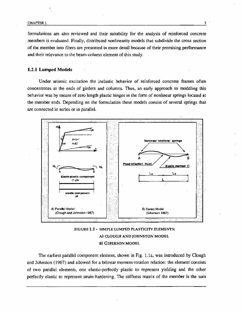
Elasto-plastlc component (1·p)k
elastic component pk
A) Parallel Model (Clough and Johnston 1967)
Nonlinear rotational springs
k ~ a. ~ A B
Filled Inflection Point
I: L
FIGURE 1.1 - SIMPLE LUMPED PLASTICITY ELEMENTS:
A) CLOUGH AND JOHNSTON MODEL
B). GIBERSON MODEL
The earliest parallel component element, shown in Fig. 1. la, was introduced by Clough
and Johnston (1967) and allowed for a bilinear moment-rotation relation: the element consists
of two parallel elements, one elastic-perfectly plastic to represent yielding and the other
perfectly elastic to represent strain-hardening. The stiffness matrix of the member is the sum
4 CHAPTER 1
of the stiffnesses of the components. Takizawa (1976) generalized this model to multilinear
monotonic behavior allowing for the effect of cracking in RC members. The series model was
formally introduc~ by Giberson (1967), although it had been reportedly used earlier. Its
original form, shown in Fig. 1.1 b, consists of a linear elastic element with one equivalent
nonlinear rotational spring attached to each end. The inelastic deformations of the member are
lumped into the end springs. This model is more versatile than the original Clough model,
since it can describe more complex hysteretic behavior by the selection of appropriate
moment-rotation relations for the end springs. This makes the model attractive for the
phenomenological representation of the hysteretic behavior of reinforced concrete members.
Several lumped plasticity constitutive models have been proposed to date (Fig. 1.2).
Such models include cyclic stiffness degradation in flexure and shear, (Clough and Benuska
1966, Takeda et al. 1970, Brancaleoni et al. 1983), pinching under reversal, (Banon et al.
1981, Brancaleoni et al. 1983) and fixed end rotations at the beam-column joint interface due
to bar pull-out (Otani 1974, Filippou and Issa 1988). Typically, axial-flexural coupling is
neglected. Nonlinear rate constitutive representations have also been generalized from the
basic endochronic theory formulation in Ozdemir (1981) to provide continuous hysteretic
relations for the nonlinear springs. An extensive discussion of the mathematical functions that
are appropriate for such models is given by Iwan (1978). A critical issue for these models is
the selection of parameters for representing the experimental hysteretic behavior of reinforced
concrete members. Two basic problems are encountered: (a) the model parameters depend not
only on the section characteristics but, also, on the load and deformation history, thus limiting
the generality of the approach, and, (b) a consistent and rational method for the selection of
model parameters requires special algorithms for ensuring a least squares fit between
analytical results and experimental data. Such an algorithm is used by Ciampi and Nicoletti
(1986) in a formal system identification method for the selection of parameters for the
moment-curvature relation proposed by Brancaleoni er'al. (1983).
The dependence of flexural strength on the axial load under uniaxial and biaxial bending
conditions has been explicitly included in the modeling of beam-columns and structural walls.
In most lumped plasticity models the axial force-bending moment interaction is described by a
yield surface for the stress resultants and an associated flow rule according to the tenets of
classical plasticity theory (Prager and Hodge 1951). The response is assumed to be linear for
stress states that fall within the yield surface in which case the flexural and axial stiffness of the
member are uncoupled and independent of the end loads. With the introduction of multiple
yield and loading surfaces and corresponding hardening rules multilinear constitutive
representations that include cracking· and cyclic stiffness degradation are possible for the
CHAPTER 1 5
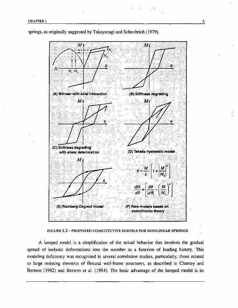
springs, as originally suggested by Takayanagi and Schnobrich (1979).
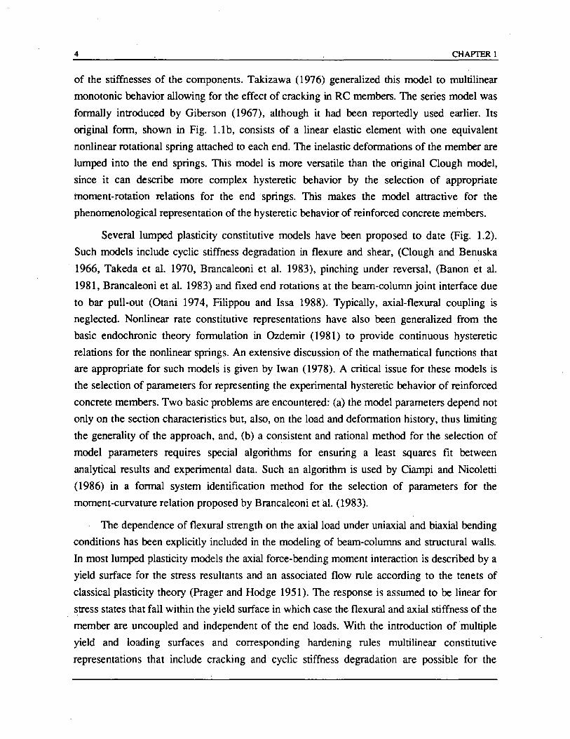
'.:',: ..... '.' ..... [.' ............ : .•. ,.: ...•..........•. < .... ' ...•.•...•... '.J ..... >' •.... dM .. de ··~,M ) ..... '\ '. "d8~~ - :.-;;: ..... ' .. ", '. ··C,',". " ••••• ', • •
.. ·{F)· •• ~.l~j.n1~·~.2~ ••• i~.·· •••••. · .• • .•• ····:·:.·· •• ' •.••••.••••••••• ·en~ClC~rohlc the~ry<,.( .... .
FIGURE 1.2 - PROPOSED CONSTITUTIVE MODELS FOR NONLINEAR SPRINGS
A lumped model is a simplification of the actual behavior that involves the gradual
spread of inelastic deformations into the member as a function of loading history. This
modeling deficiency was recognized in several correlation studies, particularly, those related
to large resisting elements of flexural wall-frame structures, as described in Charney' and
Bertero (1982) and Bertero et al ... (1984). The basic advantage of the lumped model is its
6 CHAPTER 1
simplicity that reduces storage requirements and computational cost and improves the
numerical stability of the computations. Most lumped models, however, oversimplify certain
important aspects of the hysteretic behavior of reinforced concrete members and are,
therefore, limited in applicability. One such limitation derives from restrictive a priori
assumptions for the determination of the spring parameters. Parametric and theoretical studies
of girders under monotonic loading presented by Anagnostopoulos (1981) demonstrate a
strong dependence between model parameters and the imposed loading pattern and level of
inelastic deformation. Neither factor is likely to remain constant during the dynamic response.
The problem is further accentuated by the fluctuation of the axial force in the columns.
Because of this history dependence, damage predictions at the global, but particularly at the
local level, may be grossly inaccurate. Such information can only be obtained with more
refined models capable of describing the hysteretic behavior of the section as a function of
axial load. Another limitation of most lumped plasticity models proposed to date is their
inability to describe adequately the deformation softening behavior of reinforced concrete
members. Such deformation softening can be observed as the reduction in lateral resistance of
an axially loaded cantilever column under monotonically increasing lateral tip displacement.
Again more advanced models are needed in this case.
The generalization of the rigid plastic theory concepts by Prager et al. (1951) to
reinforced concrete column stress and strain resultant variables, such as bending moment and
rotation, axial force and extension, limits the applicability of these models to well detailed
members with large inelastic deformation capacity at the critical regions. For a reinforced
concrete column section, the yield surface of the stress resultants is actually a function of a
reference strain that couples the corresponding displacement components. This contradicts
classical plasticity theory which does not account for deformation softening and assumes that
the section deformability is unlimited.
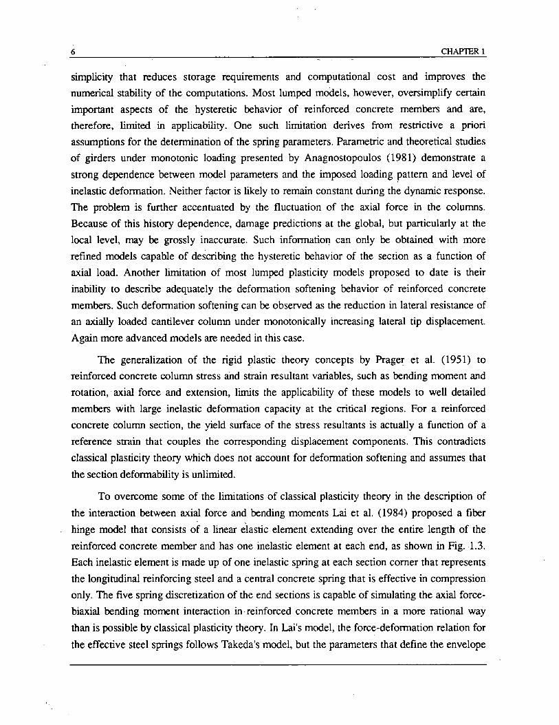
To overcome some of the limitations of classical plasticity theory in the description of
the interaction between axial force and bending moments Lai et al. (1984) proposed a fiber
hinge model that consists of a linear elastic element extending over the entire length of the
reinforced concrete member and has one inelastic element at each end, as shown in Fig.!.3.
Each inelastic element is made up of one inelastic spring at each section comer that represents.
the longitudinal reinforcing steel and a central concrete spring that is effective in compression
only. The five spring discretization of the end sections is capable of simulating the axial force
biaxial bending moment interaction in· reinforced concrete members in a more rational way
than is possible by classical plasticity theory. In Lai's model, the force-deformation relation for
the effective steel springs follows Takeda's model, but the parameters that define the envelope
CHAPTER 1
are established from equilibrium considerations.
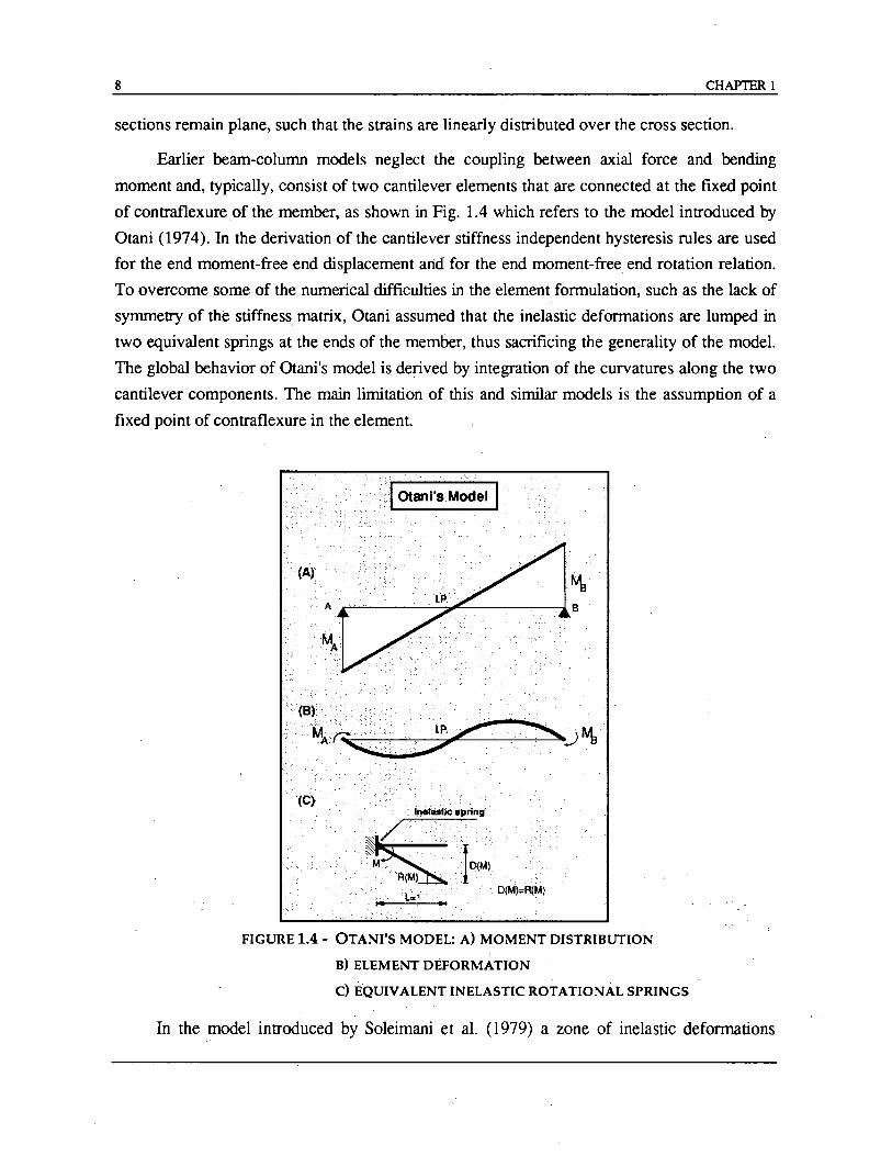
Lal'sModel
FIGURE 1.3 - LAI'S MODEL: DEGRADING INELASTIC ELEMENT FOR REINFORCED CONCRETE
BEAM-COLUMNS UNDER BIAXIAL BENDING AND AXIAL LOAD:
(A) MEMBER IN FRAME; (B) MEMBER MODEL; (C) INELASTIC ELEMENT
1.2.2 Distributed Nonlinearity Models
7
A more accurate description of the inelastic behavior of reinforced concrete members is
possible with distributed nonlinearity models. In contrast to lumped plasticity models, material
nonlinearity can take place at any element section and the element behavior is derived by
weighted integration of the section response. In practice, since the element integrals are
evaluated numerically, only the behavior of selected sections at the integration points is
monitored. Either the element deformations or the element forces are the primary unknowns
of the model and these are obtained by suitable interpolation functions from the global element
displacements or forces, respectively. Discrete cracks are represented as "smeared" over a
finite length rather than treated explicitly. The constitutive behavior of the cross section is
either formulated in accordance with classical plasticity theory in terms of stress and strain
resultants or is explicitly derived by discretization of the cross section into fibers, as is the case
in the spread plasticity fiber models. A common assumption of these models is that plane
8 CHAPTER 1
sections remain plane, such that the strains are linearly distributed over the cross section.
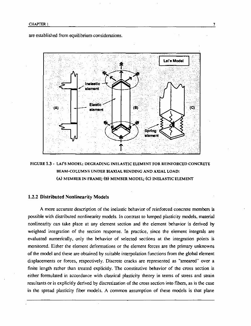
Earlier beam-column models neglect the coupling between axial force and bending
moment and, typically, consist of two cantilever elements that are connected at the fixed point
of contraflexure of the member, as shown in Fig. 1.4 which refers to the model introduced by
Otani (1974). In the derivation of the cantilever stiffness independent hysteresis rules are used
for the end moment-free end displacement and for the end moment-free end rotation relation.
To overcome some of the numerical difficulties in the element formulation, such as the lack of
symmetry of the stiffness matrix, Otani assumed that the inelastic deformations are lumped in
two equivalent springs at the ends of the member, thus sacrificing the generality of the model.
The global behavior of Otani's model is derived by integration of the curvatures along the two
cantilever components. The main limitation of this and similar models is the assumption of a
fixed point of contraflexure in the element.
. ·)1 Otanl's.Model I
n·····lP.~~j~ _ ..... _ ... ;.7._.... . .. ~
10000l L~1 . D(M)"R(M)
.1 .
FIGURE 1.4 - OTANI'S MODEL: A) MOMENT DISTRIBUTION
B) ELEMENT DEFORMATION
C) EQUIVALENT INELASTIC ROTATIONAL SPRINGS
In the model introduced by Soleimani et al. (1979) a zone of inelastic deformations
CHAPTERl 9
gradually spreads from the beam-column interface into the member as a function of loading
history. The rest of the beam remains elastic. The fixed-end rotations at the beam-column
interface are modeled through point hinges inserted at the ends of the member. These are
related to the curvature at the corresponding end section through an "effective length" factor
which remains constant during the entire response history. A very similar model was
developed by Meyer et al. (1983). The flexibility coefficients of the model are identical to
those proposed by Soleimani. A slightly different way of calculating the stiffness of the plastic
zone during reloading is proposed and Takeda's model is used to describe the hysteretic
moment-curvature relation. Fixed-end rotations are not taken into account in the study. The
original model was later extended by Roufaiel and Meyer (1987) to include the effect of shear
and axial forces on the flexural hysteretic behavior based on a set of empirical rules. The
variation of axial loads due to overturning moments is not accounted for. Darvall and Mendis
(1985) propose a similar but simpler model with end inelastic deformations defined through a
trilinear moment-curvature relation. Once formed the end hinges may remain perfectly plastic
or exhibit plastic softening or hardenirig. Perfectly plastic hinges are concentrated at a point,
while softening and hardening hinges have a user defined, finite, fixed length that is normally
assumed to be from 0.75 d to d, where d is the effective depth of the cross section.
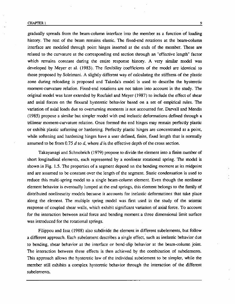
Takayanagi and Schnobrich (1979) propose to divide the element into a finite number of
short longitudinal elements, each represented by a nonlinear rotational spring. The model is
shown in Fig. 1.5. The properties of a segment depend on the bending moment at its midpoint
and are assumed to be constant over the length of the segment. Static condensation is used to
reduce this multi-spring model to a single beam-column element. Even though the nonlinear
element behavior is eventually lumped at the end springs, this element belongs to the family of
distributed nonlinearity models because it accounts for inelastic deformations that take place
along the element. The multiple spring model was first used in the study of the seismic
response of coupled shear walls, which exhibit significant variation of axial force. To account
for the interaction between axial force and bending moment a three dimensional limit surface
was introduced for the rotational springs.
Filippou and Is sa. (1988) also subdivide the element in different subelements, but follow
a different approach. Each subelement describes a single effect, such as inelastic behavior due
to bending, shear behavior at the interface or bond-slip behavior at the beam-column joint.
The interaction between these effects is then achieved by the combination of subelements.
This approach allows the hysteretic law of the individual subelement to be simpler, while the
member still exhibits a complex hysteretic behavior through the interaction of the different
subelements.
10 CHAPTER 1
'.:::,;:~} ::: . ,:,'. .. : ' .. :-. : -, " . -,' :: .:::: .:.:,.:, c,
o ~ - • '. • " • , :, •
:': .... : "":,:'. ' .: .',
:.' ~.: ' .: : - : :: . . '. :'. :,'. '.' .... ..:'" . '.-:" , -- ',' ":. . . ,-, '.. "
. . ..
. ~ ... , ....... : .. .
................ ::'\,</ •• :.'.~ ?i .. : ..... :.·::: ..
···•••·.·· •••. ··(d)·······
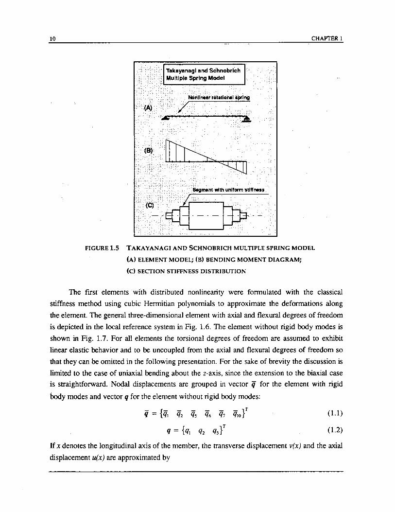
FIGURE 1.5 TAKAYANAGI AND SCHNOBRICH MULTIPLE SPRING MODEL
(A) ELEMENT MODEL; (B) BENDING MOMENT DIAGRAM;
(C) SECfION STIFFNESS DISTRIBUTION
The fIrst elements 'with distributed nonlinearity were formulated with the classical
stiffness method using cubic Hermitian polynomials to approximate the deformations along
the element. The general three-dimensional element with axial and flexural degrees of freedom
is depicted in the local reference system in Fig. 1.6. The element without rigid body modes is
shown in Fig. 1.7. For all elements the torsional degrees of freedom are assumed to exhibit
linear elastic behavior and to be uncoupled from the axial and flexural degrees of freedom so
that they can be omitted in the following presentation. For the sake of brevity the discussion is
limited to the case of uniaxial bending about the z-axis, since the extension to the biaxial case
is straightforward. Nodal displacements are grouped in vector q for the element with rigid
body modes and vector q for the element without rigid body modes:
q = {lll 112 lls 116 117 q;of
q = {ql q2 qsf
(1.1)
(1.2)
If x denotes the longitudinal axis of the member, the transverse displacement v(x) and the axial
displacement u(x) are approximated by
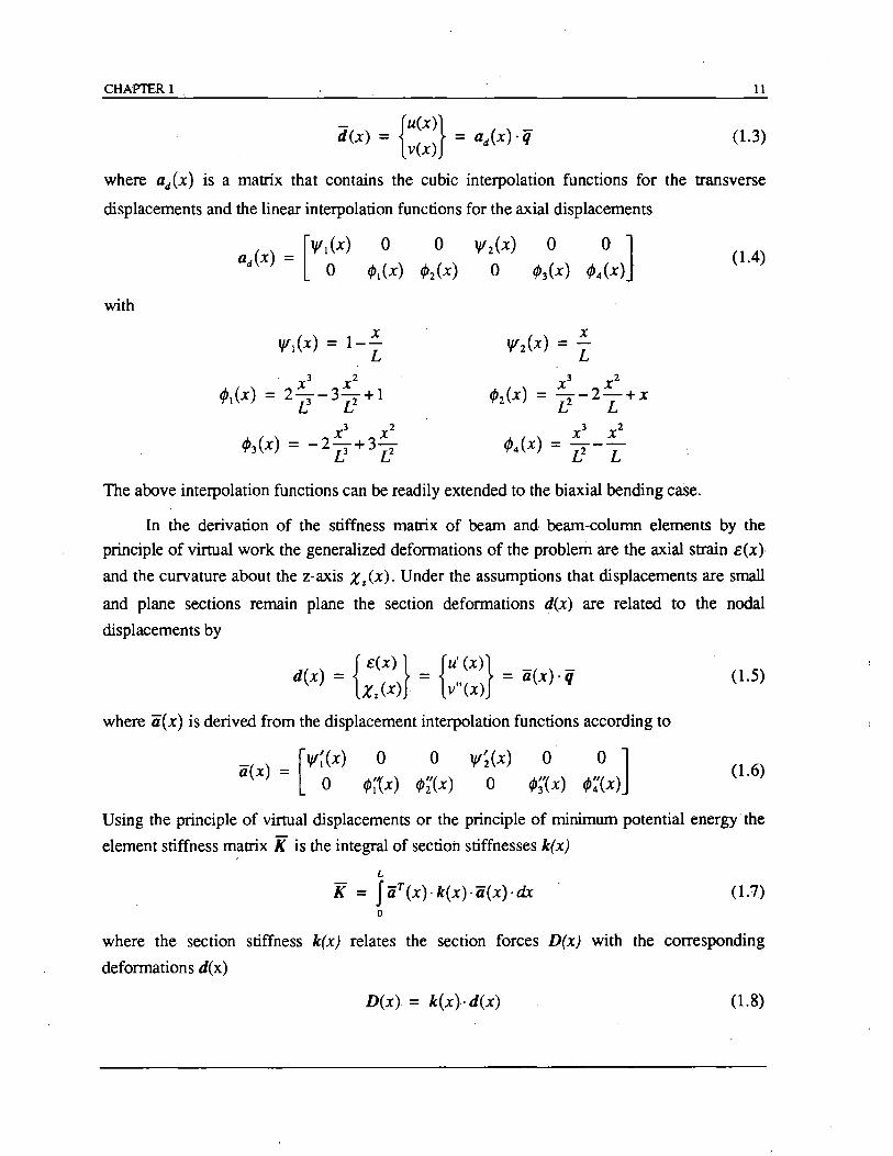
CHAPTER 1 11
d(x) = {U(X)} = aAx), if v(x)
(1.3)
where aAx) is a matrix that contains the cubic interpolation functions for the transverse
displacements and the linear interpolation functions for the axial displacements
with
x "'2(X) = -
L
The above interpolation functions can be readily extended to the biaxial bending case.
(104)
In the derivation of the stiffness matrix of beam and beam-column elements by the
principle of virtual work the generalized deformations of the problem are the axial strain e(x)
and the curvature about the z-axis X.(x). Under the assumptions that displacements are small
and plane sections remain plane the section deformations d(x) are related to the nodal
displacements by
d(x) = { e(x)} = {U1
(X)} = a(x)· if X •. (x) . v"(x)
(1.5)
where a(x) is derived from the displacement interpolation functions according to
_ [",~(X) 0 0 ",;(x) 0 0] a(x) = 0 cp~{x) cp~(x) 0 cp;(x) cp;(x)
(1.6)
Using the principle of virtual displacements or the principle of minimum potential energy -the
element stiffness matrix K is the integral of section stiffnesses k(x)
L
K = JaT(x).k(x).a(x),dx (1.7) o
where the section stiffness k(x) relates the section forces D(x) with the corresponding
deformations d(x)
D(x) = k(x)· d(x) (1.8)
12 CHAPTER 1
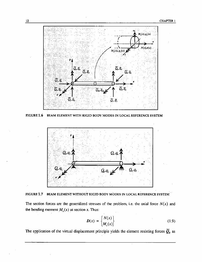
FIGURE 1.6 BEAM ELEMENT WITH RIGID BODY MODES IN LOCAL REFERENCE SYSTEM
FIGURE 1.7 BEAM ELEMENT WITHOUT RIGID BODY MODES IN LOCAL REFERENCE SYSTEM
The section forces are the generalized stresses of the problem, i.e. the axial force N{x) and
the bending moment .Mz(x) at section x. Thus:
{ N{X)}
D(x) = Mz{x) (1.9)
The application of the virtual displacement principle yields the element resisting forces QR as
CHAPTER 1 13
the integral of the section resisting forces DR(X)
L
QR = JaT(X).DR(x).dx (1.10) o
Elements based on this classical finite element displacement approach are proposed,
among· others, by Hellesland and Scordelis (1981) and Mari and Scordelis (1984). The
formulation has been extended by Bazant and Bhat (1977) to include the effect of shear by
means of multiaxial constitutive laws based on the endochronic theory. In this model the
section is subdivided into horizontal layers but each layer is allowed to crack at a different
angle that is derived from the interaction of normal and shear stress in the layer.
The main shortcoming of stiffness-based elements is their inability to describe the
behavior of the member near its ultimate resistance and after the onset of strain softening,
since they are plagued by numerical instability problems for reasons to be discussed in detail
later in this section.
Since the curvature distribution in a member that has yielded at the ends is not well
represented by cubic Hermitian interpolation functions, computational economy with
improved representation of internal deformations is achieved by the combined approximation
of, both, the section deformations, which are the basic unknowns of the problem, and the
section flexibilities. Menegotto and Pinto (1977) interpolate both variables based on the values
at a few monitored sections and include the axial force-bending moment interaction. The
section flexibilities are assumed to vary linearly between monitored sections, which is
equivalent to a hyperbolic stiffness variation. This improvement in accuracy makes the
approach computationally attractive, since fewer sections need to be monitored and, hence,
the number of variables that need to be computed and stored is smaller than in stiffness models
of comparable level of discretization.
Further improvement in element accuracy is achieved by the introduction of variable
displacement interpolation functions. A major limitation of the classical displacement approach
is the assumption of cubic interpolation functions, which result in a linear curvature
distribution along the element. This assumption leads to satisfactory results under linear or
nearly linear response. However, when the reinforced concrete member undergoes significant
yielding at the ends, the curvature distribution becomes highly nonlinear in the inelastic region.
This requires the use of a very fine discretization in the inelastic regions of stiffness-based
elements. Mahasuverachai (1982) was the first to propose the use of flexibility-dependent
shape functions that are continuously updated during the analysis as inelastic deformations
spread into the member. In his study deformation increments rather than total deformations
14 CHAPTER 1
are approximated. The section defonnation increments are written as
M(x) = I(x), h(x)· p-l . tuJ = a(x)· tuJ (1.11)
where ~ denotes the increment of the corresponding vector. This new fonnulation is,
however, applied to the development of pipeline elements where the source of nonlinearity is
geometric rather than material.
Recent efforts to develop more robust and reliable reinforced-concrete frame elements
have shown two parallel trends. First, deviating from the original classical stiffness method,
researchers have focused attention on flexibility-dependent . shape functions and, more
recently, on flexibility-based fonnulations that pennit a more accurate description of the force
distribution within the element. Secondly, the elements are sulxlivided into longitudinal fibers,
which has two inherent advantages: a) the reinforced concrete section behavior is derived
from the uniaxial stress-strain behavior of the fibers and three-dimensional effects, such as
concrete confinement by transverse steel can be incorporated into the uniaxial stress-strain
relation; and, b) the interaction between bending moment and axial force can be described in a
rational way.
The flexibility approach is based on force interpolation functions within the element.
~ypically, the element is analyzed without including the rigid body modes. In this case the end
rotations relative to the chord and the axial differential displacement are the element
generalized defonnations, or simply, element defonnations. The element forces and
defonnations without the rigid body modes are shown in Fig. 1.7. Under the assumption of
small defonnations and small displacements the element defonnations q are related to the
element displacements if in Fig. 1.6 by the compatibility matrix. In the uniaxial bending case
the vector of element forces without rigid body modes is
_ (1.12)
It is common to assume that the bending moment distribution inside the element is linear and
that the axial force distribution is constant: In vector notation:
D(x) = b(x)· Q (1.13)
where b(x) is a matrix containing the force interpolation functions
o 1
] (1.14) o
The application of the virtual force principle yields the element flexibility
CHAPTER 1 15
L
F = J bT (X)· I(x)· b(x)· dx (1.15) o
where I(x) is the section flexibility matrix, such that:
d(x) = I(x), D(x) (1.16)
The advantage of this formulation stems from the realization that, irrespective of the
state of the element, the force interpolation functions in Eqs. (1.13) and (1.14) satisfy the
element equilibrium is a strict sense, as long as no element loads are applied. In other words,
whatever material nonlinearities take place at the section level and even as the element starts
softening when deformed beyond its ultimate resistance, the assumed internal force
distributions are exact.
A critical issue in flexibility-based elements is the implementation in an existing finite
element program. Computer programs are typically based on the direct stiffness method of
analysis. In this case the solution of the global system of equilibrium equations for the given
loads yields the unknown structural displacements. After the element displacements are
extracted from the structural displacements the phase of element state determination starts.
During this phase the resisting forces and the stiffness matrix need to be determined for the
given element displacements. The element state determination requires a special procedure in
a flexibility-based element, since the element resisting forces cannot be derived by integration
of the section resisting forces according to Eq. (1.10). An interesting state determination
procedure for a flexibility-based finite element is proposed in Ciampi and Carlesimo (1986)
and is discussed at length in Spacone et al. (1992). The section moment-curvature relation of
this model is based on the endochronic theory presented in Brancaleoni et al. (1983). The
element state determination is based on the section deformation residuals that result from the
numerical integration of the section constitutive relation. The interaction between axial force
and bending moment is not included in the latter model.
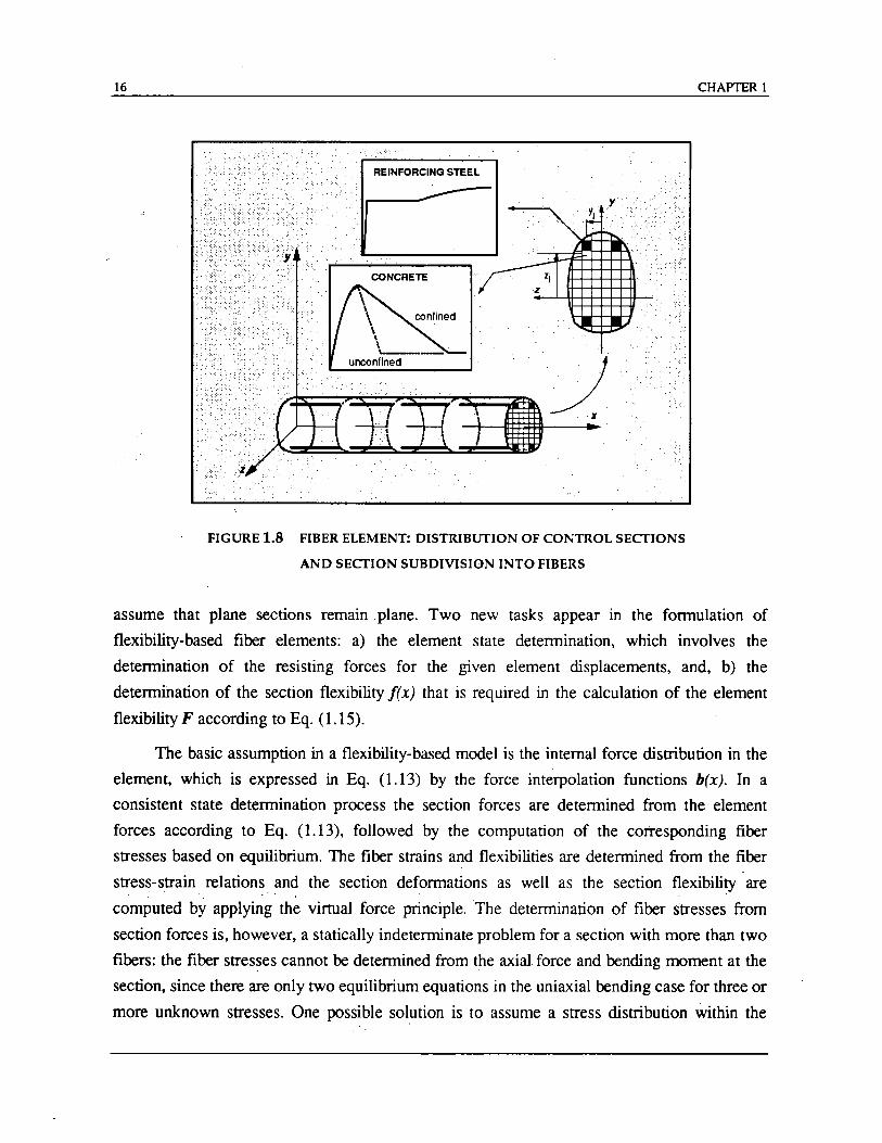
1.2.3 Fiber Models
The most promising models for the nonlinear analysis of reinforced concrete members
are, presently, flexibility-based fiber elements. In these models the element is subdivided into
longitudinal fibers, as shown in Fig. 1.8. The geometric characteristics of the fiber are its location in the local y, z reference system and the fiber area Ai/ib' The constitutive relation of
the section is not specified explicitly, but is derived by integration of the response of the fibers,
which follow the uniaxial stress-strain relation of the particular material, as shown in Fig. 1.8.
The elements proposed to date are limited to small displacements and deformations and
16
FIGURE 1.8 FIBER ELEMENT: DISTRIBUTION OF CONTROL SECTIONS
AND SECTION SUBDIVISION INTO FIBERS
CHAPTER 1
assume that plane sections remain plane. Two new tasks appear in the formulation of
flexibility-based fiber elements: a) the element state determination, which involves the
determination of the resisting forces for the given element displacements, and, b) the
determination of the section flexibility f(x) that is required in the calculation of the element
flexibility F according to Eq. (1.15).
The basic assumption in a flexibility-based model is the internal force distribution in the
element, which is expressed in Eq. (1.13) by the force interpolation functions b(x). In a
consistent state determination process the section forces are determined from the element
forces according to Eq. (1.13), followed by the computation of the corresponding fiber
stresses based on equilibrium. The fiber strains and flexibilities are determined from the fiber
stress-strain relations and the section deformations as well as the section flexibility are
computed by applying' th~ virtual force principle. The determination of fiber stresses from
section forces is, however, a statically indeterminate problem for a section with more than two
fibers: the fiber stresses cannot be determined from the axial. force and bending moment at the
section, since there are only two equilibrium equations in the uniaxial bending case for three or
more unknown stresses. One possible solution is to assume a stress distribution within the
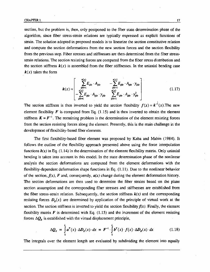
CHAPTER 1 17
section, but the problem is, then, only postponed to the fiber state detennination phase of the
algorithm, since fiber stress-strain relations are typically expressed as explicit functions of
strain. The solution adopted in proposed models is to linearize the section constitutive relation
and compute the section defonnations from the new .section forces and the section flexibility
from the previous step. Fiber stresses and stiffnesses are then detennined from the fiber stress
strain relations: The section resisting forces are computed from the fiber stress distribution and
the section stiffness k(x) is assembled from the fiber stiffnesses. In the uniaxial bending case
k(x) takes the fonn
k(x) =
,,(x)
L,Eijib .~ ijib=l
"(x)
- L, Eijib . Aijib . YiJib iJib=1
II(X)
- L.,Eijib . ~ . Yijib ijib=l
11(.1)
L., Eijib ·Aijib . Y~ ijib=l
(1.17)
, The section stiffness is then inverted to yield the section flexibility I(x) = k-1(x).The new
element flexibility F is computed from Eq. (1.15) and is then inverted to obtain the element
stiffness K = F-1 . The remaining problem is the detennination of the element resisting forces
from the section resisting forces along the element. Presently, this is the main challenge in the
development of flexibility-based fiber elements.
The first flexibility-based fiber element was proposed by Kaba and Mahin (1984). It
follows the outline of the flexibility approach presented above using the force interpolation
functions b(x) in Eq. (1.14) in the detennination of the element flexibility matrix. Only uniaxial
bending is taken into account in this model. In the state detennination phase of the nonlinear
analysis the section defonnations are computed from the element defonnations with the
flexibility-dependent defonnation shape functions in Eq. (1.11). Due to the nonlinear behavior
of the section,f(x), F and, consequently, a(x) change during the element defonnation history.
The section defonnations are then used to detennine the fiber strains based on the plane
section assumption and the corresponding fiber stresses and stiffnesses are established from
the fiber stress-strain relation. Subsequently, the section stiffness k(x) and the corresponding
resisting forces DR(x) are detennined by application of the principle of virtual work at the
section. The section stiffness is inverted to yield the section flexibility f(x); Finally, the element
flexibility matrix F is detennined with Eq. (1.15) and the increment of the element resisting
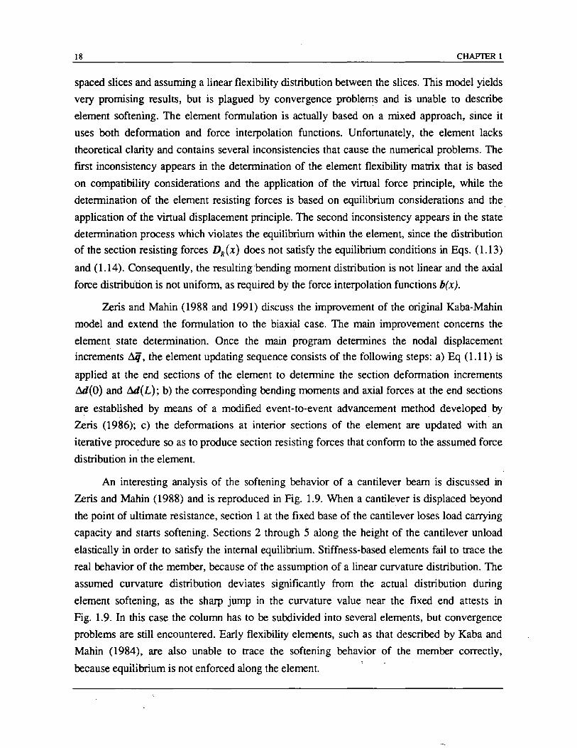
forces llQR is established with the virtual displacement principle,
L L
llQR = J aT (x)· llDR(x)· dx = F-1 -J bT (x)· I(x)· llDR(x)· dx ( 1.18) o 0
The integrals over the element length are evaluated by subdividing the element into equally
18 CHAPTER 1
spaced slices and assuming a linear flexibility distribution between the slices. This model yields
very promising results, but is plagued by convergence problems and is unable to describe
element softening. The element formulation is actually based on a mixed approach, since it
uses both deformation and force interpolation functions. Unfortunately, the element lacks
theoretical clarity and contains several inconsistencies that cause the numerical problems. The
first inconsistency appears in the determination of the element flexibility matrix that is based
on compatibility considerations and the application of the virtual force principle, while the
determination of the element resisting forces is based on equilibrium considerations and the
application of the virtual displacement principle. The second inconsistency appears in the state
determination process which violates the equilibrium within the element, since the distribution
of the section resisting forces DR{x) does not satisfy the equilibrium conditions in Eqs. (1.13)
and (1.14). Consequently, the resulting bending moment distribution is not linear and the axial
force distribution is not uniform, as required by the force interpolation functions b(x).
Zeris and Mahin (1988 and 1991) discuss the improvement of the original Kaba-Mahin
model and extend the formulation to the biaxial case. The main improvement concerns the
element state determination. Once the main program determines the nodal displacement
increments !iq, the element updating sequence consists of the following steps: a) Eq (1.11) is
applied at the end sections of the element to determine the section deformation increments
.&I{O) and .&I(L); b) the correspondIng bending moments and axial forces at the end sections
are established by means of a modified event-to-event advancement method developed by
Zeris (1986); c) the deformations at interior sections of the element are updated with an
iterative procedure so as to produce section resisting forces that conform to the assumed force
distribution in the element.
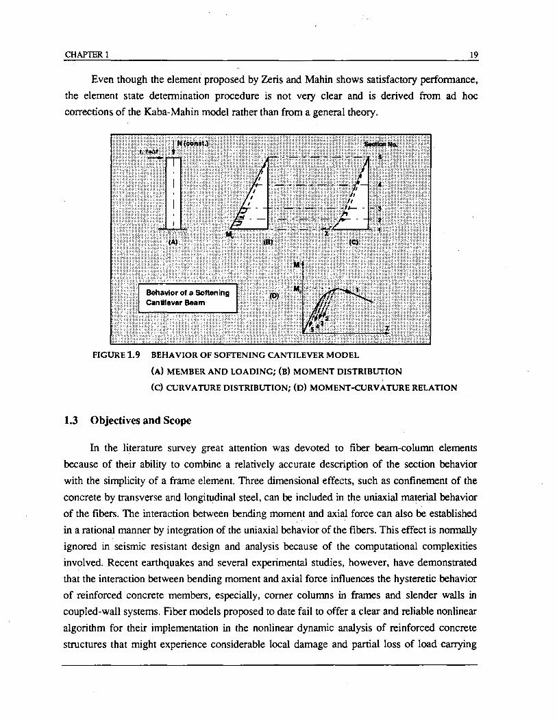
An interesting analysis of the softening behavior of a cantilever beam is discussed in
Zeris and Mahin (1988) and is reproduced in Fig. 1.9. When a cantilever is displaced beyond
the point of ultimate resistance, section 1 at the fixed base of the cantilever loses load carrying
capacity and starts softening. Sections 2 through 5 along the height of the cantilever unload
elastically in order to satisfy the internal equilibrium. Stiffness-based elements fail to trace the
real behavior of the member, because of the assumption of a linear curvature distribution. The
assumed curvature distribution deviates significantly from the actual distribution during
element softening, as the sharp jump in the curvature value near the fixed end attests in
Fig. 1.9. In this case the column has to be subdivided into several elements, but convergence
problems are still encountered. Early flexibility elements, such as that described by Kaba and
Mahin (1984), are also unable to trace the softening behavior of the member correctly,
because equilibrium is not enforced along the element.
CHAPTER 1 19
Even though the element proposed by Zeris and Mahin shows satisfactory perfonnance,
the element state detennination procedure is not very clear and is derived from ad hoc
corrections of the Kaba-Mahin model rather than from a general theory.
FIGURE 1.9 BEHAVIOR OF SOFTENING CANTILEVER MODEL
(A) MEMBER AND LOADING; (B) MOMENT DISTRIBUTION
(c) CURVATURE DISTRIBUTION; (D) MOMENT<URVATURE RELATION
1.3 Objectives and Scope
In the literature survey great attention was devoted to fiber beam-column elements
because of their ability to combine a relatively accurate description of the section behavior
with the simplicity of a frame element. Three dimensional effects, such as confinement of the
concrete by transverse and longitudinal steel, can be included in the uniaxial material behavior
of the fibers. The interaction between bending moment and axial force can also be established
in a rational manner by integration of the uniaxial behavior of the fibers. This effect is normally
ignored in seismic resistant design and analysis because of the computational complexities
involved. Recent earthquakes and several experimental studies, however, have demonstrated
that the interaction between bending moment and axial force influences the hysteretic behavior
of reinforced concrete members, especially, comer columns in frames and slender walls in
coupled-wall systems. Fiber models proposed to date fail to offer a clear and reliable nonlinear
algorithm for their implementation in the nonlinear dynamic analysis of reinforced concrete
structures that might experience considerable local damage and panial loss of load carrying
20 CHAPTER 1
capacity.
The present study proposes a new fiber beam-column finite element along with a
consistent nonlinear solution algorithm that is particularly suitable for the analysis of the highly
nonlinear hysteretic behavior of softening members, such as reinforced concrete columns
under varying axial load. The element formulation is cast in the framework of the mixed
method, but can be equally derived with a flexibility approach. The proposed element state
determination is based on a nonlinear iterative algorithm that always maintains equilibrium and
compatibility within the element and that eventually converges to a state that satisfies the
section constitutive relations within a specified tolerance.
The main objectives of this study are:
• to present a formal mixed method framework for the formulation of a beam-column
element using force interpolation functions and flexibility-dependent deformation shape
functions;
• to introduce an innovative and numerically robust state determination procedure for
flexibility-based beam-column elements. This procedure is based on an iterative process
for the determination of resisting forces from the given element deformations that
always maintains equilibrium and compatibility within the element. Even though the
procedure is discussed in the present study in the context of a fiber beam-column model,
it is equally applicable to any nonlinear constitutive relation for the section;
• to discuss important numerical aspects of the element implementation in a general
purpose analysis. program, with emphasis on the aspects that relate to the
implementation of the element state determination procedure;
• to extend the element formulation to include the application of element loads. This
rather important topic has received scant attention in seismic response studies of
reinforced concrete buildings. It is especially relevant for the extension of the proposed
mOdel to prestressed concrete structures;
• to illustrate with a series of examples the ability of the proposed model to describe the
hysteretic behavior of reinforced concrete members. The response sensitivity to the
number of control sections in the element and the effect of the selected tolerance on the
accuracy of the results is discussed in a few parameter studies.
Following the review of previous relevant studies in this chapter, Chapter 2 presents the
mixed formulation of the beam-column element and illustrates the proposed nonlinear solution
algorithm for the element state determination. Chapter 3 extends the formulation to the case

CHAPTER 1 21 /~ ~~~~----------------~---------------------------------------------
of a fiber beam-column element and discusses material models for the nonlinear stress-strain
relation of the fibers. In Chapter 4 issues related to the numerical implementation of the
nonlinear solution algorithm are discussed along with the associated convergence criteria. A
consistent method for the application of element loads in flexibility based finite elements is
also presented in this chapter. The response sensitivity to the number of control sections in the
element and the effect of the convergence tolerance on the accuracy of the results is discussed
in a few parameter studies at the beginning of Chapter 5. The validity of the proposed model
is then established by comparing the analytical results with information from experimental
studies. The conclusions of this study and directions for future research are presented in
Chapter 6.

CHAPTER 2
FORMULATION OF BEAM-COLUMN ELEMENT
2.1 General
This chapter presents the general formulation of a beam-column finite element based on
the flexibility method. The presentation is cast in the more general form of a mixed method for
two reasons: (a) this approach illustrates better the state-determination process used in the
nonlinear analysis algorithm, and, (b) it yields in a direct way the flexibility dependent
deformation shape functions of the element that reduce the general mixed method formulation
to the flexibility method used in this study. In addition, the generality of the mixed method
allows the exploration of alternative deformation shape functions in future studies.
In keeping with the generality of the presentation the force-deformation relation is not
specialized at the section leveL This is deferred to the following chapter where the section
force-deformation relation is derived from a fiber discretization of the cross section. A
"different approach which uses the theory of classical plasticity to derive a hysteretic model of
the section force-deformation relation is presented by Spacone et aL (1992).
The proposed beam-column element is based on the assumption that deformations are
small and that plane sections remain plane during the loading history. The formulation of the
element is based on the mixed method: the description of the force distribution within the
element by interpolation functions that satisfy equilibrium is the starting point of the
formulation. Based on the concepts of the mixed method it is shown that the selection of
flexibility dependent shape functions for the deformation field of the element results in
considerable simplification of the final equations. With this particular selection of deformation
shape functions the general mixed method reduces to the special case of the flexibility method.
The mixed method formalism is, nonetheless, very useful in understanding the proposed
procedure for the element state determination.
The proposed formulation offers several advantages over previous models:
• Equilibrium and compatibility are always satisfied along the element: equilibrium is
satisfied by the selection of force interpolation functions and compatibility is satisfied by
integrating the section deformations to obtain the corresponding element defonnations
23
24 CHAP1ER 2
and end displacements. An iterative solution is then used to satisfy the nonlinear section
force-defonnation relation within the specified tolerance.
• The softening response of reinforced concrete members,. which are either poorly
reinforced or are subjected to high axial forces, can be described without computational
difficulties.
In the first part of the chapter, after the definition of generalized element forces and
corresponding element defonnations, the mixed method fonnulation of the element is
presented. The second part focuses on the element state detennination process and the step
by-step calculation of the element resisting forces that correspond to given element
defonnations. These derivations are made without reference to a specific section model. This
is deferred to Chapter 3, where the nonlinear procedure is specialized to a fiber section model.
2.2 Definition of Generalized Forces and Deformations
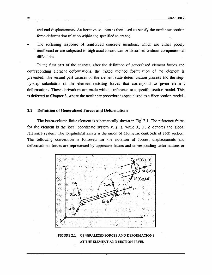
The beam-column finite element is schematically shown in Fig. 2.1. The reference frame
for the element is the local coordinate system x, y, Z, while X, Y, Z denotes the global
reference system. The longitudinal axis x is the union of geometric centroids of each section.
The following convention is followed for the notation of forces,·· displacements and
defonnations: forces are represented by uppercase letters and corresponding defonnations or
FIGURE 2.1 GENERALIZED FORCES AND DEFORMATIONS
AT THE ELEMENT AND SECTION LEVEL
CHAPTER 2 25
displacements are denoted by the same letter in lowercase. Normal letters denote scalar
quantities, while boldface letters denote vectors and matrices.
Fig. 2.1 shows the element forces with the corresponding deformations. Rigid body
modes are not included in Fig. 2.1. Since the present formulation is based on linear geometry,
rigid body modes can be incorporated with a simple geometric transfonnation. The element has 5 degrees of freedom: one axial extension, qs' and two rotations relative to the chord at
each end node, (ql, q3) and (q2' q4)' respectively. For the sake of clarity these are called
element generalized defonnations or simply element defonnations in the following discussion.
Q1 through Qs indicate the corresponding generalized forces: one axial force, Qs' and two
bending moments at each end node QI' Q3 and Q2' '4, respectively. The end rotations and
corresponding moments refer to two arbitrary, orthogonal axes y and z. The element
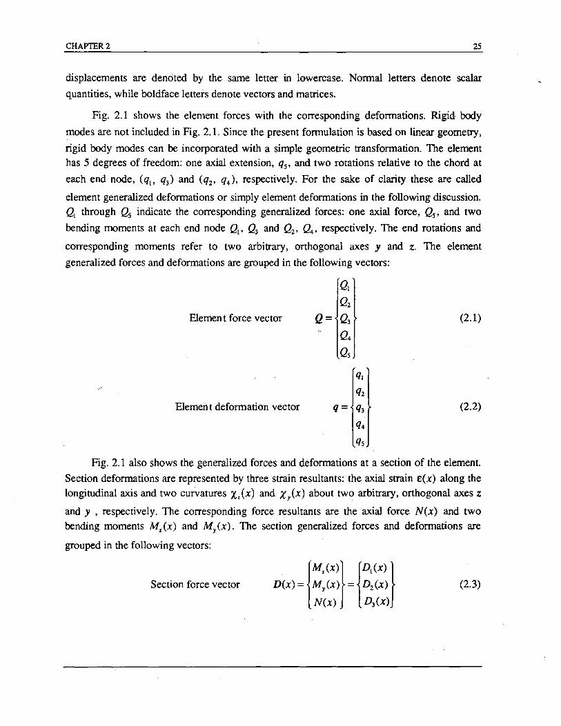
generalized forces and defonnations are grouped in the following vectors:
Q1
Q2 Elemen t force vector Q= Q3 (2.1)
'4 Qs
ql
q2
Elemen t defonnation vector q= % (2.2)
q4
qs
Fig. 2.1 also shows the generalized forces and defonnations at a section of the element.
Section defonnations are represented by three strain resultants: the axial strain E(X) along the
longitudinal axis and two curvatures Xz(x) and Xy(x) about two arbitrary, orthogonal axes z
and y , respectively. The corresponding force resultants are the axial force N(x) and two bending moments Mz (x) and My (x). The section generalized forces and defonnations are
grouped in the following vectors:
Section force vector {
MZ(X)} {DI (x) } D(x) = M/x) = D2 (x)
N(x) D3(x)
(2.3)
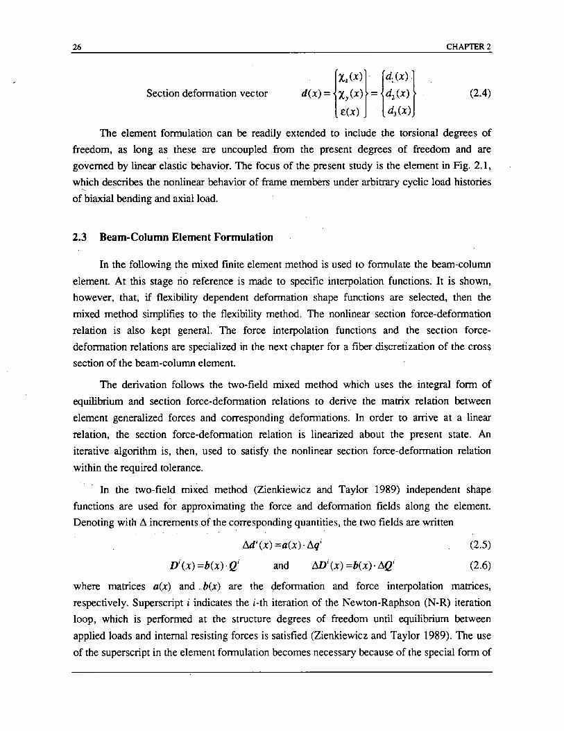
26 CHAPTER 2
Section deformation vector (2.4)
The element formulation can be readily extended to include the torsional degrees of
freedom, as long as these are uncoupled from the present degrees of freedom and are
governed by linear elastic behavior. The focus of the present study is the element in Fig. 2.1,
which describes the nonlinear behavior of frame members under arbitrary cyclic load histories "
of biaxial bending and axial load.
2.3 Beam-Column Element Formulation
In the following the mixed finite element method is used to formulate the beam-column
element. At this stage rio reference is made to specific interpolation functions. It is shown,
however, that, if flexibility dependent deformation shape functions are selected, then the
mixed method simplifies to the flexibility method. The nonlinear section force-deformation
relation is also kept general. The force interpolation functions and the section force
deformation relations are specialized in the next chapter for a fiber discretization of the cross
section of the beam-column element.
The derivation follows the two-field mixed method which uses the integral form of
equilibrium and section force-deformation relations to derive the matrix relation between
element generalized forces and corresponding deformations. In order to arrive at a linear
relation, the section force-deformation relation is linearized about the present state. An
iterative algorithm is, then, used to satisfy the nonlinear section force-deformation relation
within the required tolerance.
In the two-field mixed method (Zienkiewicz and Taylor 1989) independent shape
functions are used for approximating the force and deformation fields along the element.
Denoting with ~ increments of the corresponding quantities, the two fields are written
fuf(x) =a(x). ~qi
and Mi (x) =b(x). ~Qi
(2.5)
(2.6)
where matrices a(x) and .b(x) are the deformation and force interpolation matrices,
respectively. Superscript i indicates the i-th iteration of the Newton-Raphson (N-R) iteration
loop, which is performed at the structure degrees of freedom until equilibrium between
applied loads and internal resisting forces is satisfied (Zienkiewicz and Taylor 1989). The use
of the superscript in the element formulation becomes necessary because of the special form of
CHAPTER 2 27
the deformation interpolation functions, which are flexibility dependent.
In the mixed method formulation the integral forms of equilibrium and section force
deformation relations are expressed first. These are then combined to obtain the relation
between element force and deforniation increments.
The weighted integral form of the linearized section force-deformation relation is
L J aDT (x)· [rui(x) - i-I (x) . Mi(x)]dx=O (2.7) o
The section force-deformation relation appears in the flexibility form
so that the resulting element flexibility matrix is symmetric, as discussed by Zienkiewicz and
Taylor (1989). The superscript i-I indicates that at the i-th Newton-Raphson iteration the
section flexibility at the end of the previous iteration is used. Substituting Eqs. (2.5) and (2.6)
in Eq. (2.7) results in
L
OQT. J bT (x)· [a(x). L~I/ - i-I (x)· b(x)· ~Qi]dx=O o
Since Eq. (2.8) must hold for any OQT, it follows that
The expressions in square brackets represent the following matrices:
F'-' =[! bT (X) 1'-' (X) " b(x)"dx ]
T=[!bT(X)"Q(X)"dx ]
(2.8)
(2.10)
(2.11)
where F is the element flexibility matrix and T is a matrix that only depends on the
interpolation function matrices. Using Eqs. (2.10) and (2.11) Eq. (2.9) can be written in the
form
(2.12)
or equivalently
(2.13)
This is the matrix expression of the integral form of the linearized section force-deformation
28 CHAPTER 2
relation.
In the next step the equilibrium of the beam element is satisfied. In the classical two
field mixed method the integral form of the equilibrium equation is derived from the virtual
displacement principle
L
f&lT(X).[Di-1(X)+Mi(x)]-dX =&/.pi (2.14) o
where pi is the vector of applied loads that are in equilibrium with the internal forces
D i-
1 (x) + Mi(x). Eqs. (2.5) and (2.6) are substituted in Eq. (2.14) to yield
&/.[! aT (x).[b(x) .Q'-' +b(x)· t.{!]. dx] = f>qT·r
Observing that Eq. (2.15) must hold for arbitrary 8qT, it follows that
[! aT (x)· b(x)·dx lQ'-' + [t aT(x)· b(x)· dx 1 t.Q' = r
If the notation introduced in Eq. (2.11) is used, Eq. (2.16) can be written in matrix form
(2.15)
(2.16)
(2.17)
This is the matrix expression of the integral form of the element equilibrium equations. The
rearrangement and combination of Eqs. (2.12) and (2.17) results in
[_F
i
-
1 r] {!:!.Qi} { 0 } . rT O·!:!.qi = pi _ rT . Qi-I (2.18)
If the first equation in Eq. (2.18) is solved for !:!.Qi and the result is substituted in the second
equation, the following expression results
(2.19)
So far, the specific selection of force and deformation interpolation functions b(x) and a(x),
respectively, has not been addressed. In keeping with the generality of the formulation the
selection of the force interpolation functions b(x) is deferred to the following chapter. Even
though in a mixed finite element method the deformation interpolation functions a(x) are
completely independent of b(x), Eq. (2.11) reveals that a special choice of the deformation
shape functions a(x) results in considerable simplification. With this simplification in mind a(x)
are selected as flexibility dependent shape functions according to the following expression
a(x) = /-1 (x)· b(x)· [Fi-l r (2.20)
CHAPTER 2 29
These interpolation functions, thus, relate the section deformations with the corresponding
element deformations according to
(2.21)
F i-
I is the tangent element flexibility matrix at the end of the previous Newton-Raphson
iteration. This special selection of the deformation shape functions reduces matrix T in
Eq. (2.11) to a 3,,3 identity matrix I. This can be readily proven by substituting Eq. (2.20) in
Eq. (2.11):
With this choice of the deformation shape functions a(x) Eq. (2.19) becomes
[ Fi- I r . !J.qi = P -:- Qi-I
(2.22)
(2.23)
At the same time this choice of functions a(x) reduces the general mixed method to the
flexibility method. The final matrix equation,Eq. (2.23), expresses the linearized relation
between the applied unbalanced forces P - Qi-I and the corresponding deformation
increments !J.qi at the element level. The element stiffness matrix is written in the form [Ft to indicate that it is obtained by inverting the element. flexibility matrix. The linear equation
system in Eq. (2.23) is different from that obtained by the classical stiffness method in two
respects: (a) the element stiffness matrix is obtained by inverting the element flexibility matrix,
as in the flexibility method, and, (b) the state determination phase of the nonlinear analysis is
different, as will be described in detail in the following section.
Even though the classical flexibility method yields the same system of linearized
equations in Eq. (2.23), the above derivation was based on the two-field mixed method for the
following reasons: (a) the mixed method formulation yields directly the expression for the
flexibility dependent deformation shape functions a(x) in Eq. (2.20), (b) it reveals the
consistent implementation of the state determination process, and, (c) it is more general in
scope allowing alternative deformation shape functions to be explored in future studies.
Since a(x) is not independent of hex) and changes during the iterative solution process,
as is apparent from Eq. (2.20), the proposed method corresponds to the classical flexibility
method. Moreover, this procedure reduces to the stiffness method for the case that the section
constitutive relation is perfectly linear. In other words, the independence between the two
fields is not intrinsic in the definition of the shape functions, but derives from the material
nonlinearity of the section force-deformation relation.
30 CHAPTER 2
2.4 State Determination
Most studies to date concerned with the analysis of reinforced concrete frame structures
are based on finite element models that are derived with the stiffness method. Recent studies
have focused on the advantages of flexibility based models (Zeris and Mahin 1988), but have
failed to give a clear and consistent method of calculating the resisting forces from the given
element deformations. This problem arises when the formulation of a finite element is based
on the application of the virtual force principle. While the element is flexibility-dependent, the
computer program into which it is inserted is based on the direct stiffness method of analysis.
In this case the solution of the global equilibrium equations yields the displacements of the
structural degrees of freedom. During the phase of state determination the resisting forces of
all elements in the structure need to be determined. Since in a flexibility based element there
are no deformation shape functions to relate the deformation field inside the element to the
end displacements (or element deformations) this process is not straightforward and is not
well developed in flexibility based models proposed to date. This fact has led to· some
confusion in the numerical implementation of previous models. The description of the
consistent state determination process in this study benefits from the derivation of the
governing equations by the two-field mixed method.
In a nonlinear structural analysis program each load step corresponds to the application
of an external load increment to· the structure. The corresponding structural displacement
increments are determined and the element deformations are extracted for each element. The
process of finding the resisting forces that correspond to the given element deformations is
known as state determination. The state determination process is made up of two nested
phases: a) the element state determination, when the element resisting forces are determined
for the given end deformations, and b) the structure state determinarion, when the element
resisting forces are assembled to the structure resisting force vector. The resisting forces are
then compared with the total applied loads and the difference, if any, yields the unbalanced
forces which are then applied to the structure in an iterative solution process until external
loads and internal resisting forces agree within a specified tolerance.
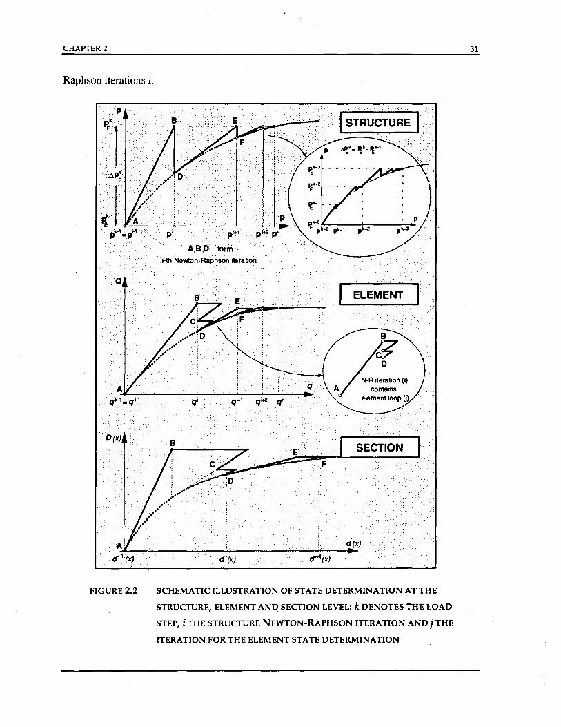
In the present study the nonlinear algorithm consists of three distinct nested processes,
whiCh are illustrated in Fig. 2.2. The two outermost processes denoted by indices k and i
involve structural degrees of freedom· and correspond to classical nonlinear analysis
procedures. The innermost process denoted by index j is applied within each element and
corresponds to the element state determination. Fig. 2.2. shows the evolution of the structure,
element and section states during one load increment ~p; that requires several Newton-
CHAPTER 2
Raphson iterations i.
FIGURE 2.2 SCHEMATIC ILLUSTRATION OF STATE DETERMINATION ATTHE
STRUCTURE, ELEMENT AND SECTION LEVEL: k DENOTES THE LOAD
STEP, i THE STRUCTURE NEWTON-RApHSON ITERA nON AND j THE
ITERATION FOR THE ELEMENT STATE DETERMINATION
31
32 CHAPTER 2
. In summary, the superscripts of the nested iterations are defined as follows:
k denotes the applied load step. The external load is imposed in a sequence of load
increments ~p:. At load step k the total external load is equal to P: = p:-I + ~p: with
k= l, ... ,nstep and P~ = 0;
i denotes the Newton-Raphson iteration scheme at the structure level, i.e. the structure
state determination process. This iteration. loop yields the structural displacements pk
that correspond to applied loads P;;
j denotes the iteration scheme at the element level, i.e. the element state determination
process. This iteration loop is necessary for the determination of the element resisting
forces that correspond to element deformations qi during the i-th Newton-Raphson
iteration.
The processes denoted by indices k and i are common in nonlinear analysis programs
and will not be discussed further. The iteration process denoted by the index j, on the other
hand, is special to the _beam~column element formulation developed in this study and will be
described in detail. It should be pointed out that any suitable nonlinear solution algorithm can
be used for the iteration process denoted by index i. In this study the Newton-Raphson
method is used. The selection of this method for iteration loop i does not affect the strategy
for iteration loop j, which has as its goal the determination of the element resisting forces for
the given element deformations.
In a finite element that is based on the stiffness method of analysis the section
deformations are obtained directly from the element end deformations by deformation
interpolation functions. The corresponding section resisting forces are determined
subsequently from the section force-deformation relation. The weighted integral of the section
resisting forces over the element length yields the element resisting forces and completes the
process of element state determination.
In a flexibility-based finite element the first step is the determination of the element
forces from the current element deformations using the stiffness matrix at the end of the last
iteration. The force interpolation functions yield the forces along the element. The first
problem is, then, the determination of the section deformations from the given section forces,
since the nonlinear section force-deformation relation is commonly expressed as an explicit
function of section deformations. The second problem arises from the fact that changes in the
section stiffness produce a new element stiffness matrix which, in tum, changes the element
forces for the given deformations.
CHAPTER 2 33
These problems are solved in the present study by a special nonlinear solution method.
In this method residual element deformations are determined at each iteration. Deformation
compatibility at the structural level requires that these residual deformations be corrected.
This is accomplished at the element level by applying corrective element' forces based on the
current stiffness matrix. The corresponding section forces are determined from the force
interpolation functions so that equilibrium is always satisfied along the element. These section
forces cannot change during the section state determination in order to maintain equilibrium
along the element. Consequently, the 'linear approximation of the section force-deformation
relation about the present state results in residual section deformations. These are then
integrated along the element to obtain new residual element deformations and the whole
process is repeated until convergence occurs. It is imponant to stress that compatibility of
element deformations and equilibrium along the element are always satisfied in this process.
The nonlinear solution procedure for the element state determination is schematically
illustrated in Fig. 2.3 for one Newton-Raphson iteration i. In Fig. 2.3 convergence in loop j is
reached in three iterations. The consistent notation between Figs. 2.2 and 2.3 highlights the
relation between the corresponding states of the structure, the element and the section, which
are denoted by uppercase Roman letters.
At the i-th Newton-Raphson iteration it is necessary to determine the element resisting
forces for the current element deformations
qi = qi-I + llqi
To this end an iterative process denoted by index j is introduced inside' the' i-th Newton
Raphson iteration. The first iteration corresponds to j= 1. The initial state of the element,
. represented by point A and j=O in Fig. 2.3, corresponds to the state at the end of the last
iteration of loop j for the (i-I) Newton-Raphson iteration. With the initial element tangent
stiffness matrix
and the given element deformation increments .
llqj=1 = llqi
the corresponding element force increments are:
llQj=1 = [Fj=ot .6qj=1
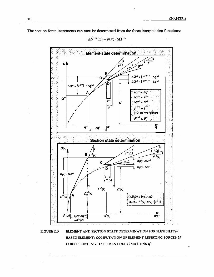
34 CHAPlER2
The-section force increments can now be determined from the force interpolation functions:
/illj=1 (x) = b(x). ~Qj=l-
FIGURE 2.3
Q~' ...
........ •....••
.. i I ,.
....
Q'-11 .. IQ' -.. t:.q __
.. ' .. : ... :. "
d
> Llqi-1:.z t:.fj ----&,ia2~, SI~1
&r~=-~
Ft=o= F~L ',', ....
_]=3:eonver'gence --Fi~'3=FI
Q
-Sectioh st&ttfctetermlnatlcm
c ?~:::====:j : '·:··>LJD .... I ,..-....
.. .. ••• / ,i-2(x}
.......
cf1(X} I .. s(x}' t:.ql-:I t:.dl·Yx}
d(x}
o (x)
I
~ '59-ri ~' b(x}' t:.01-2
b(x}' t:.Oia3
d(x}
ELEMENT AND SECTION STATE DETERMINATION FOR FLEXIBILITY
BASED ELEMENT: COMPUTATION OF ELEMENT RESISTING FORCES !! CORRESPONDING TO ELEMENT DEFORMATIONS qi
CHAPTER 2 35
With the section flexibility matrix at the end of the previous Newton-Raphson iteration
the linearization of the section force-deformation relation yields the section defonnation increments Mi=I(X):
Mi=I(X) = li=o(x). MJi=\x)
The section deformations are updated to the state that corresponds to point B in Fig. 2.3:
d i=l(X) = di=O(x) + ~di=l(X)
According to the section force-deformation relation, which is here -assumed to be
explicitly known for simplicity's sake, section deformations d i=l(X) correspond to resisting
forces Dt1(X) and a new tangent flexibility matrix li=l(x) (Fig. 2.3). In a finite element based
on the stiffness method the section resisting forces Dk=l(X) would be directly transformed to
element resisting forces Qi=l thus violating the equilibrium along the element in a strict sense.
Since this is undesirable, a new nonlinear solution method is proposed in this study. In this
approach the section unbalanced forces are first determined
Dt=l(X) = Di=I(X)_ Dr (x)
and are then transformed to residual section deformations ri=l(x)
r i=1 (x) = li=1 (x)· v:.,=1 (x) (2.24)
The residual section deformations are thus the linear approximation to the deformation error
made in the linearization of the section force-deformation relation (Fig. 2.3). While any
suitable flexibility matrix can be used in calculating the residual deformations, the tangent
flexibility matrix used in this study offers the fastest convergence rate.
The residual section deformations are integrated along the element based on the virtual
force principle to obtain the residual element deformations:
L
si=l = J bT (x)· ri=l(x)· dx o
(2.25)
At this point the first iteration j= 1 of the corresponding iteration loop is complete. The final
element and section states for j= 1 correspond to point B in Fig. 2.3. The residual section deformations ri=l(x) and the residual element deformations Si=1 are determined in the first
iteration, but the corresponding deformation vectors are not updated. Instead, they are the
starting point of the remaining steps within iteration loop j. The presence of residual element
deformations Sf=l violates compatibility, since elements sharing a common node would now
have different end displacements. In order to restore the inter-element compatibility corrective
36 CHAPTER 2
forces equal .to -[ Fi=1 r . Si=1 must be applied at the ends of the element, where FJ=1 is the
updated element tangent flexibility matrix detennined by integration of the section flexibility
matrices according to Eq. (2.10). A corresponding force increment -b(x)· [Fi=1 r . Si=1 is
applied at all control sections inducing a defonnation in~ement _/i=l(x).b('x).[pJ=lr ·S}=I.
Thus, in the second iteration j=2 the state of the element and of the sections within the
element change as follows: the eiement forces are updated to the value
QJ=2 = QJ=1 + ~ Qi=2
where
. ~ Qi=2 = -[ Fi=1 r . si=1
and the section forces and defonnations are updated to the values
. IJi=2 (x) = Di=1 (x) + mi=2 (x)
and
where
m i=2 (x) = -b(x) . [ Fi=1 r . Si=1
Mi=2(X) = r i =1 (x)- /i=I(X)' b(x)· [FJ=1 r . Si=1
The state of the element and the sections within the element at the end of the second iteration
j=2 corresponds to point C in Fig. 2.3. The new tangent flexibility matrices /i=2(X) and. the
new residual section defonnations
ri=2(x) = /i=2(X)' D£=2(X)
are computed for all sections. The residual section defonnations are then integrated to obtain
the residual element deformations Si=2 and the new element tangent flexibility matrix Fi=2 is
detennined by integration of the section flexibility matrices /i=2(X) according to Eq. (2.10).
This completes the second iteration within loop j.
The third and subsequent iterations follow exactly the same scheme. Convergence is
achieved ,when the selected cO~1Vergence criterion is satisfied, as discussed in more detail in
Chapter 4. With the conclusion of iteration loop) the element resisting forces for. the given
deformationsqi are established, as represented by point D in Figs. 2.2 and 2.3. The Newton-
Raphson iteration process can now proceed with step i+ 1 .
It is important to point out that during iteration' loop j the element deformations qi do
CHAPTER 2 37
not change except in the fIrst iteration j= 1, when increments 6qi=l = /1qi are added to the
element defonnations qi-I at the end of the previous Newton-Raphson iteration. These
defonnation increments result from the application of corrective loads /1P~ at the structural
degrees of freedom during the Newton-Raphson iteration process. For j> 1 only the element
forces change until the nonlinear solution procedure converges to the element resisting forces
Qi which correspond to element defonnations qi. This is illustrated at the top of Fig. 2.3
where points B, C and D, which represent the state of the element at the end of subsequent
iterations in loopj, lie on the same vertical line, while the corresponding points at the control
sections of the element do not, as shown in the bottom of Fig. 2.3. This feature of the
proposed nonlinear solution procedure ensures displacement compatibility at the element ends.
The proposed nonlinear analysis method offers several advantages. Equilibrium along
the element is always strictly satisfied, since section forces are derived from element forces by
the force interpolation functions according to Eq. (2.6). Compatibility is also satisfIed, not
only at the element ends, but also along the element. In fact, in the expression for the section
defonnation corrections
Mi (x) = ri-\x) - 1'-1 (x)· h(x)· [Fi-I r . sj-I
the second term satisfIes Eqs. (2.20) and (2.21), which express the relation between section
and element defonnations by means of shape functions a(x). The residual section
defonnations ri-I(x), however, do not strictly satisfy this compatibility condition. It is possible
to satisfy this requirement by integrating the residual defonnations r j-
I (x) to obtain si-I and
then using the defonnation shape functions a(x) to calculate the section deformation
increments as a(x)· Si-l. Since this is, however, rather ineffIcient from a computational
standpoint, the small compatibility error in the calculation of residual section defonnations
r j-
I (x) is neglected in this study.
While equilibrium and compatibility are satisfIed along the element during each iteration
of loop j, the section force-deformation relation and, consequently, the element force
deformation relation is only satisfIed within a specifIed tolerance when convergence is
achieved at point D in Fig. 2.3. In other words, during subsequent iterations the element
forces approach the value that corresponds to the imposed element deformations, while
maintaining equilibrium and compatibility along the element at all times. This approximation of
the force-deformation relation in the proposed nonlinear analysis method is preferable to the
approximation of either the equilibrium or the compatibility conditions of the element,
particularly when considering the uncertainty in the definition of constitutive relations for
reinforced concrete structures.
38 CHAPTER 2
2.5 Summary of Nonlinear Solution Algorithm
After the description of the element state determination process in the previous section a
step-by-step summary of the computations is presented below. The summary focuses on a
single iteration i at the structural degrees of freedom, because the innovative aspect of the
present study is the process of element state determination. The rest of the nonlinear solution
algorithm follows well established methods, such as the Newton-Raphson method selected in
this study. Alternative solution strategies can be implemented without additional effort, since
these are independent of the "element state determination. The relation of the Newton-Raphson
iteration· to the nonlinear solution of the entire structure is illustrated at the top of Fig. 2.2,
which also shows the relation between the overall solution strategy and the element state
determination process with corresponding states denoted by uppercase Roman letters. Fig. 2.3
shows in detail the evolution of the state determination process for an element and
corresponds to steps (4) through (13) in the following summary. The flow chart of
computations for the entire solution algorithm is shown in Fig. 2.4, while the flow chart of
computations for the element state determination is shown in Fig. 2.5.
The i-th Newton-Raphson iteration is organized as follows:
(1) Solve the global system of equations and update the structural displacements.
At the i-th Newton-Raphson iteration the structure stiffness matrix K:-1 at the end of the
previous iteration i-I is used to compute the displacement increments ~pi for the given
load increments ~P~ which represent the unbalanced forces from the previous iteration.
Ki-I . ~pi = ~pi s " E (2.26)
(2.27)
(2) Calculate the element deformation increments and update the element deformations.
Using matrix Lele , which relates structural displacements with element deformations, the
element deformation increments !!JJi are determined:
Ani = L . ~pi ~ .Ie (2.28)
(2.29)
Note that matrix Lei. is the combination of two transformations: in the fIrst
transformation the element displacements in the global reference system p are
transformed to the displacements q in the element local refer~nce system. In the second
transformation the element displacements q are transformed to element deformations q
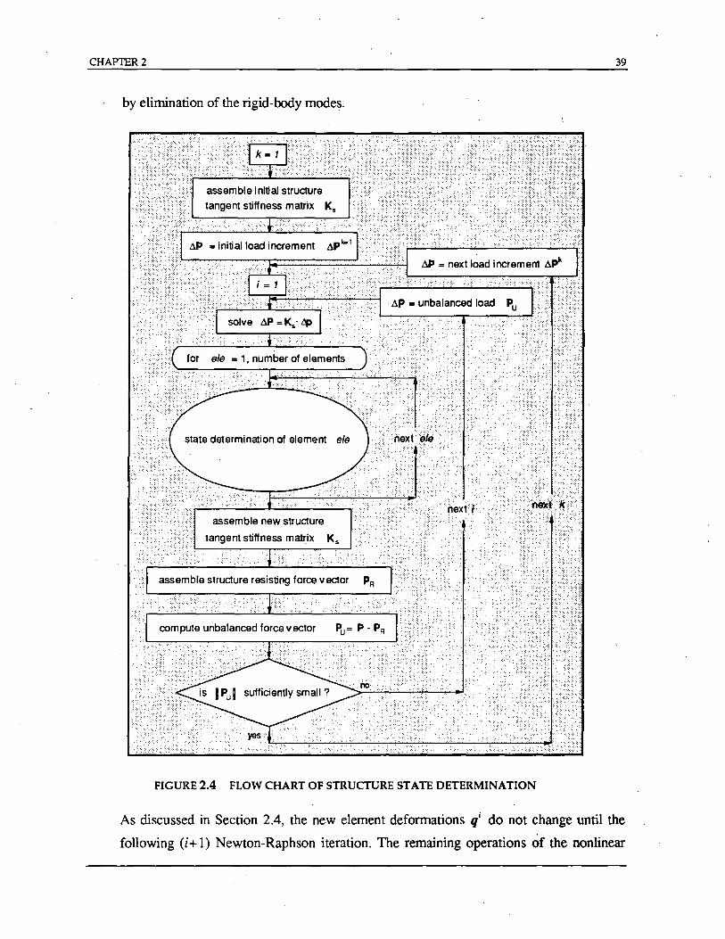
CHAPTER 2 39
by elimination of the rigid-body modes.
FIGURE 2.4 FLOW CHART OF STRUCTURE STATE DETERMINATION
As discussed in Section 2.4, the new element defonnations qi do not change until the
following (i+ 1) Newton-Raphson iteration. The remaining operations of the nonlinear
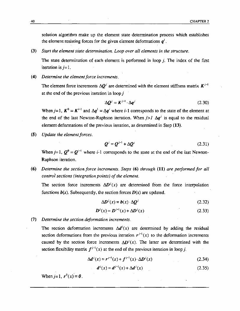
-40 CHAPTER 2
solution algorithm make up the element statedetennination process which establishes
the element resisting forces for the given element defonnations qi .
(3) Start the element state determination. Loop over all elements in the structure.
The state detennination of each element is perfonned in loop j. The index of the fIrst
iteration is}= 1.
(4) Determine the element force increments.
The element force increments I!!..Qj are detennined with the element stiffness matrix K j-I
at the end of the previous iteration in loop}
(2.30)
When}= 1, KO = K i-I and I!!..ql = 4qi where i-I corresponds to the state of the element at
the end of the last Newton-Raphson iteration. When}> 1 I!!..qj is equal to the residual
element defonnations of the previous iteration, as detennined in Step (13).
(5) Update the elementforces.
(2.31)
When}= 1, QO = Qi-I where i-I corresponds to the state at the end of the last Newton
Raphson iteration.
(6) Determine the section force increments. Steps (6) through (11) are performed for all
control sections (integration points) of the element.
The section force increments Wi (x) are detennined from the force interpolation
functions b(x). Subsequently,. the section forces D(x) are updated.
Wi (x) = b(x) . I!!..Qi
Dj (x) = Dj-I (x) + wj (x)
(7) Determine the section deformation increments.
(2.32)
(2.33)
The section defonnation increments I!!..Li(x) are detennined by adding the residual
section defonnations from the previous iteration. r i- I (x) to the defonnation increments
caused by the section force increments Wj(x). The latter are detennined with the
section flexibility matrix / i-I (x) at the end of the previous iteration in loop j.
When}= 1, rO(x) = O.
Mi (x) = r i - I (x) + /j-I(X)' Wi (x)
d j (x) = d j-
I (x) + &Ii (x)
(2.34)
(2.35)
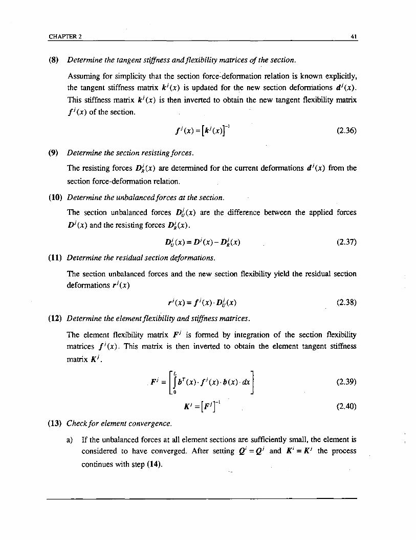
CHAPTER 2 41
(8) Determine the tangent stiffness and flexibility matrices of the section.
Assuming for simplicity that the section force~deformation relation is known explicitly,
the tangent stiffness matrix k i (x) is updated for the new section deformations d i (x).
This stiffness matrix k i (x) is then inverted to obtain the new tangent flexibility matrix
Ii (x) of the section.
(2.36)
(9) Determine the section resisting forces.
The resisting forces D~(x) are determined for the current deformations di(x) from the
section force-deformation relation.
(10) Determine the unbalancedforces at the section.
The section unbalanced forces Dt(x) are the difference between the applied forces
Di (x) and the resisting forces D~(x).
(2.37)
(11) Determine the residual section deformations.
The section unbalanced forces and the new section flexibility yield the residual section
deformations ri (x)
ri (x) = Ii (x)· D&<x)
(12) Determine the element flexibility and stiffness matrices.
(2.38)
The element flexibility matrix Fi is formed by integration of the section flexibility
matrices Ii (x). This matrix is then inverted to obtain the element tangent stiffness
Fi; [IbT(x)"r(X)"b(X)"dx]
Ki=[Fir
(13) Checkfor element convergence.
(2.39)
(2.40)
a) If the unbalanced forces at all element sections are sufficiently small, the element is considered to have converged. After setting Qi = Qi and Ki = K i the process
continues with step (14).
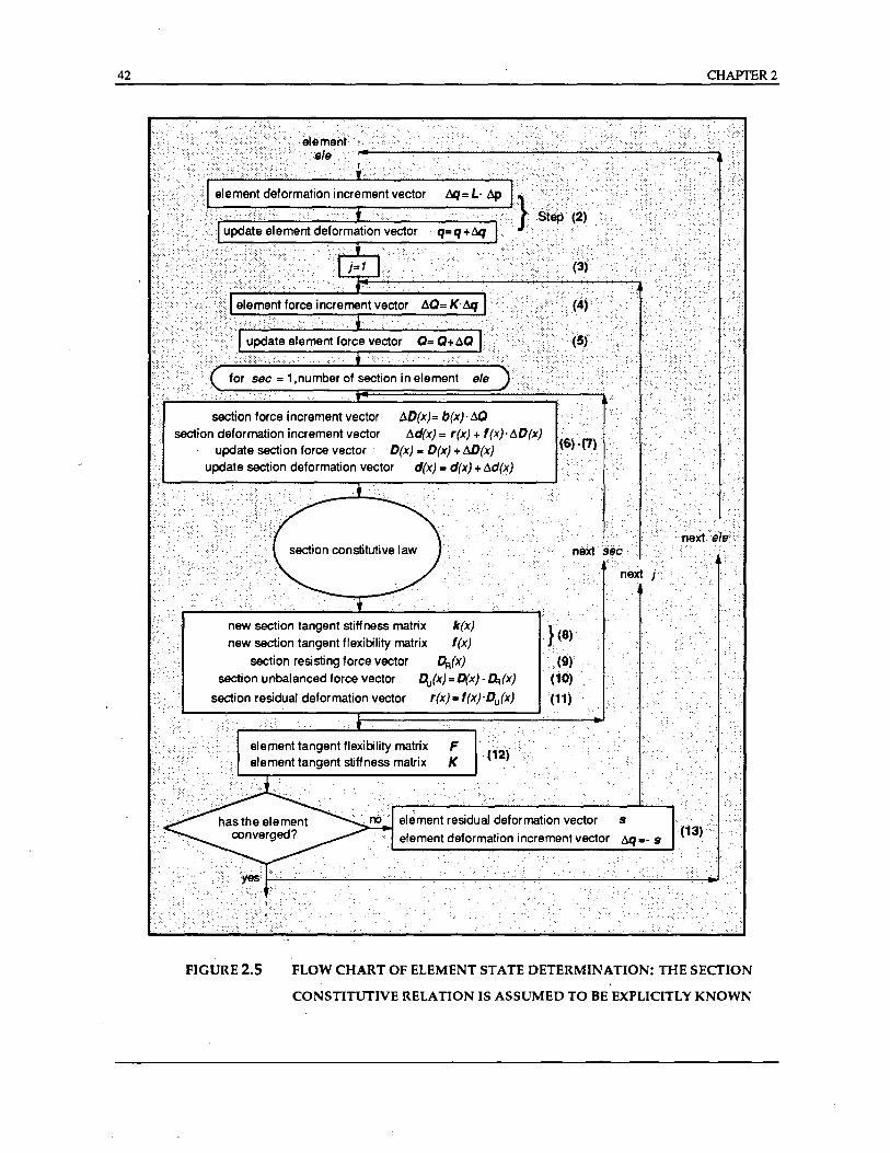
42
~D(x)= b(x)· 6Q ~d(x) = r(x) + f(x)- ~D(x)
D(x) = D(x) + ~D(x) d(x) = d(x) + 6d(x)
k(x)
f(x)
~(x)
new section tangent stiffness matrix new section tangent flexibility matrix
section resisting force vector
section unbalanced force vector ~(x) = D(x) -~(x)
r(x) = f(x)-Du(x)
CHAPTER 2
FIGURE 2.5 FLOW CHART OF ELEMENT STATE DETERMINATION: THE SECTION
CONSTITUTIVE RELATION IS ASSUMED TO BE EXPLICITLY KNOWN
CHAPTER 2 43
b) If some sections have not converged, the residual element deformations sj are
determined by integration of the residual section deformations r j (x).
(2.41)
At this point j is incremented to j+ 1 and a new iteration begins in loop j. In this case 6qj in Eq. (2.30) is replaced with 6qj+! which is set equal to - sj
(2.42)
and steps (4) through (13) are repeated until convergence is achieved at all sections of
the element.
(14) Determine the resisting forces and the new stiffness matrix of the entire structure.
When all elements have converged, the i-th step of the Newton-Raphson iteration is
complete. The element forte vectors are assembled to form the updated structure
resisting forces
II
i ~ T ( .) PR = ~Lele' (! de (2.43) ele=l
where n is the total number of beam-column elements in the structure and the subscript
ele is added as a summation index. The new structure stiffness matrix is formed by
assembling the current element stiffness matrices
(2.44) ele=l
At this point the structure resisting forces P~ are compared with the total applied loads.
If the difference ~P~, which is the structure unbalanced force vector, is not within the
specified tolerance, i is incremented to i+ 1 and the next Newton-Raphson iteration begins. Steps (1) through (14) are repeated after replacing ~P~ with LW~+l = LW~ until
convergence takes place at the structure degrees of freedom.
A graphical overview of. the entire nonlinear analysis procedure is presented in Figs. 2.4
and 2.5. Fig. 2.4 provides an overview of the entire process with the nesting of the individual
iteration loops and does not differ from conventional nonlinear analysis schemes. The new
features of the algorithm are introduced in the element state determination phase, which is
singled out for presentation in Fig. 2.5. Since all integrations along the element in Eqs. (2.39)
and (2.41) need to be performed numerically, an additional iteration loop over all control
sections of the element is introduced in this diagram. The actual numerical implementation is
44 CHAPTER 2
deferred to Chapter 4.
In the interest of clarity the above presentation of the nonlinear analysis procedure refers
to an explicit section. defonnation relation. The following chapter addresses the
implementation of this algorithm in the context of a fiber beam-column element. In the latter
case the section force-defonnation relation is not explicitly known, but is derived from the
stress-strain relation of the fibers that the section is divided into.
CHAPTER 3
REINFORCED CONCRETE FIBER BEAM-COLUMN ELEMENT
3.1 General
In the previous chapter a beam-column element was formulated based on the flexibilitY
method of analysis. For clarity of presentation the section force-deformation relation was
assumed explicitly known, but no further details about the constitutive model were discussed
in order to demonstrate the general character of the proposed method. In this chapter the
proposed method is specialized to a beam-column element composed of longitudinal fibers for
which the section force-deformation relation is established by integration of the uniaxial
stress-strain behavior of the fibers.
The element is based on the assumption that plane sections remain plane and normal to
the reference axis during the deformation history. This leads to a simple ge<?metric relation
between section generalized deformations and fiber strains. The nonlinear character of the
element derives entirely from the nonlinear fiber stress-strain relations (material nonlinearity).
The element formulation is based on the formal framework of the mixed method, as described
in the previous chapter. The deformation interpolation matrix has the same flexibility
dependent form as discussed in Chapter 2, while the force interpolation matrix is selected to
represent linear bending moment and constant axial force distribution along the element. This
form is exact when no element lo~ds are present. The latter case is dealt with in Chapter 4,
where a procedure is proposed for the consistent inclusion of element loads in the context of
the flexibility method.
The fiber element state determination is identical to the procedure presented at length in
Chapter 2. In the fiber beam-column element, however, the section force-deformation relation
is only implicitly known as a function of the stress-strain relation and the deformation history
of the fibers. Correspondingly, a few steps need to be added to the procedure in Section. 2.5
for the section state determination, which determines the section force and new tangent
stiffness matrix for the given section deformations.
Following a definition of new variables that the discretization of the cross section into
fibers introduces, the material models for describing the hysteretic behavior of the fibers are
45
46 CHAPTER 3
discussed. Subsequently, the element state detennination for the fiber section model is
presented in detail and the chapter concludes with a brief summary of the entire nonlinear
analysis algorithm, with highlights of the new steps that are introduced by the fiber . . . .
discretization of the cross section.
3.2 Model Assumptions
The fonnulation of the fiber beam-column element is based on the assumption of linear
geometry. Plane sections remain plane and nonnal to the longitudinal axis during the element
defonriation history. While this hypothesis is acceptable for small defonnations of elements
composed of homogeneous materials, it does not properly account for phenomena which are
characteristic of reinforced concrete elements, such as cracking and bond-slip. The effect of
cracking and tension stiffenil'1g can be included in the model by an appropriate modification of
the stress-strain relation of reinforcing steel or concrete according to the smeared crack
concept of finite element analysis. This effect is only significant in the pre-yield phase of
response and can be neglected in studies which focus on the hysteretic behavior under large
inelastic defonnationreversals. By contrast, the contribution of bond-slip to the element
deformations increases with the magnitude and number of loading cycles. The inclusion of
bond-slip deformations in an element that· is based on section behavior is a challenging
problem, whiCh is beyond the scope of the present study. Shear effects are also neglected,
which is a reasonable approximation for medium to large span to depth ratios of the member.
From the assumption that plane sections remain plane and nonnal to the longitudinal
axis, all"fiber strains and stresses act parallel to this axis. Since the reference axis is fixed, this
implies that the geometric centroids of the sections fonn a straight line that coincides with the
reference axis. If an element does not comply with this hypothesis, it should be divided into
subelements that connect the centroids of the selected sections.
The accuracy of the element response and, consequently, that of the entire structure are
affected by the mesh selection, that is the number of sections used in the discretization of a
given member, and by the number of fibers in a section. A large number of fibers certainly
gives better results, but computational cost increases with it, since the history variables
necessary to track the hysteretic behavior of each fiber must be stored at each iteration. The
selection of the optimum number and location of fibers and the optimum number of
integration points along the element axis is beyond the scope of this study.
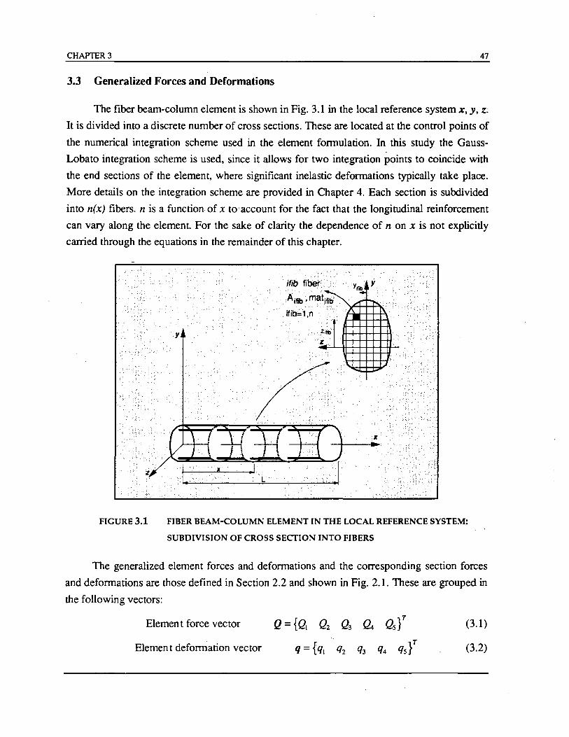
CHAPTER 3 47
3.3 Generalized Forces and Deformations
The fiber beam-column element is shown in Fig. 3.1 in the local reference system x, y, z;
It is divided into a discrete number of cross sections. These are located at the control points of
the numerical integration scheme used in the element formulation. In this study the Gauss
Lobato integration scheme is used, since it allows for two integration points to coincide with
the end sections of the element, where significant inelastic deformations typically take place.
More details on the integration scheme are provided in Chapter 4. Each section is subdivided
into n(x) fibers. n is a function of x to'account for the fact that the longitudinal reinforcement
can vary along the element. For the sake of clarity the dependence of n on x is not explicitly
carried through the equations in the remainder of this chapter.
FIGURE 3.1 FIBER BEAM-COLUMN ELEMENT IN THE LOCAL REFERENCE SYSTEM:
SUBDIVISION OF CROSS SECTION INTO FIBERS
The generalized element forces and deformations and the corresponding section forces
and deformations are those defined in Section 2.2 and shown in Fig. 2.1. These are grouped in
the following vectors:
Elemen t force vector
Elemen t deformation vector
Q Q n QS}T 2 3 lo4 (3.1)
(3.2)
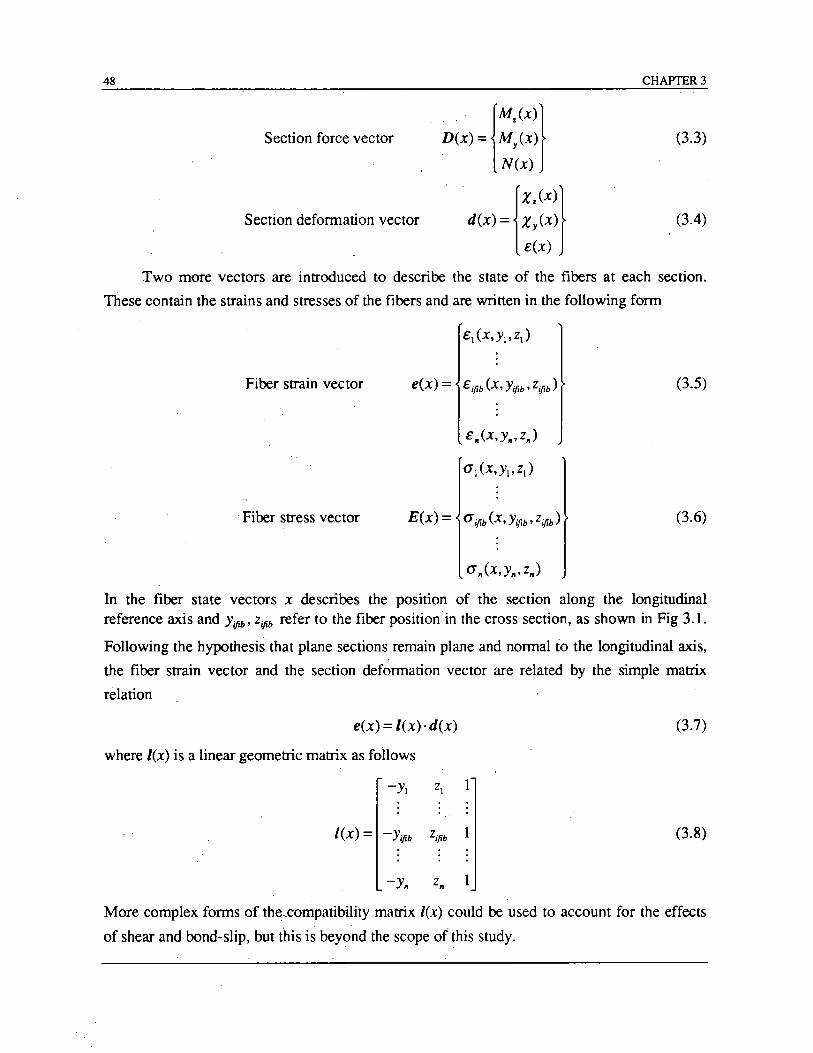
48 CHAPTER 3
Section force vector D(x) = {::~:~} N(x)
(3.3)
Section defonnation vector d(x) = {~:~:~} c;(x)
(3.4)
Two more vectors are introduced to describe the state of the fibers at each section.
These contain the strains and stresses of the fibers and are written in the following fonn
Fiber strain vector (3.5)
Fiber stress vector (3.6)
(J "(x,y,,, z,,)
In the fiber state vectors x describes the posIlIon of the section along the longitudinal reference axis and Yifib' Zijib refer to the fiber position in the cross section, as shown in Fig 3.1.
Following the hypothesis that plane sections remain plane and nonnal to the longitudinal axis,
the fiber strain vector and the section defonnation vector are related by the simple matrix
relation
e(x) = l(x)' d(x) (3.7)
where lex) is a linear geometric matrix as follows
-Yl Zl 1
lex) = -Yijib zifib 1 (3.8)
-Y" z" 1
More complex fonns of the£ompatibility matrix lex) could be used to account for the effects
of shear and bond-slip, but this is beyond the scope of this study.
CHAPTER 3 49
3.4 Fiber Constitutive Models
The nonlinear behavior of the proposed fiber beam-column element derives entirely
from the nonlinear behavior of the fibers. Thus, the validity of the analytical results depends
on the accuracy of the fiber material models. Since the present study is limited to the
hysteretic behavior of reinforced concrete members and the effect of bond-slip is neglected,
only two material models are required: one for concrete and one for reinforcing steel. The
element formulation simplifies the task of material model selection to uniaxial behavior, which
is thoroughly studied and well established to date. Three-dimensional effects on material
behavior can be included into the uniaxial model by appropriate modification of the
parameters that define the monotonic envelope. This is imponant in the case of concrete,
where confinement by transverse and longitudinal reinforcement has a significant effect on the
stress-strain behavior.
The models used in the present study are those discussed in Filippou et a1. (1983). While
the reinforcing steel model in Filippou et al. (1983) remains one of the most accurate and
convenient to use, many improved confined concrete models have been proposed in the last
ten years (Mander et a1. 1988, Sheikh and Yeh 1990). Still, the model used in this study offers
a good compromise between simplicity and accuracy and remains an excellent choice for the
hysteretic behavior of concrete. Comparisons between analytical and experimental results in
Chapter 5 demonstrate that for RC beam-column elements under small axial loads the
concrete material model shows satisfactory accuracy. In any case the modular program
architecture that underlies the proposed beam-column element allows for the easy exchange of
material models and a more extensive material library will be developed in the near future.
It is important to note that both stress-strain models are explicit functions of strain. This
is a significant feature of the material models in connection with the proposed fiber model,
where fiber strains are determined from section deformations according to Eq. (3.7). The
stress determination only involves a function evaluation based on the current fiber stress and
strain and the given strain increment. This reduces the computational effort considerably
relative to material models that are not explicit functions of strain, such as the well-known
Ramberg-Osgood steel model.
3.4.1 Steel Stress-Strain Relation
The reinforcing steel stress-strain behavior is described by the nonlinear model of
Menegotto and Pinto (1973), as modified by Filippou et a1. (1983) to include isotropic strain
hardening. The model is computationally efficient and agrees very well with experimental
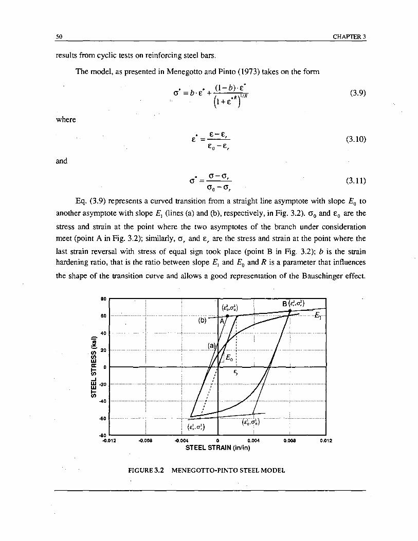
50
results from cyclic tests on reinforcing steel bars.
The model, as presented in Menegotto and Pinto (1973) takes on the fonn
where
and
• b • (l-b)·c· 0' = . c + 1/R
.. (l+coR
)
• c- c, c =---''-
• 0'-0', 0' =--'-
0'0-0',
CHAPTER 3
(3.9)
(3.10)
(3.11)
Eq. (3.9) represents a curved transition from a straight line asymptote with slope Eo to
another asymptote with slope E1 (lines (a) and (b), respectively, in Fig. 3.2). 0'0 and Eo are the
stress and strain at the point where the two asymptotes of the branch under consideration
meet (point A in Fig. 3.2); similarly, 0', and E, are the stress and strain at the point where the
last strain reversal with stress of equal sign took place (point B in Fig. 3.2); b is the strain hardening ratio, that is the ratio between slope E1 and Eo and R is a parameter that influences
the shape of the transition curve and allows a good representation of the Bauschinger effect.
80~------~--------------~------~------~~----~
B (~,d.)
60
40 ................ .
j U; 20 U) W
i ... _.- ••.••.•. ", "i
(b)
....... ~-.. .
~ Or-------~------~----~~--~--~~~--~------~ t; ..J Hi ·20 •................
t; -40
-60 .............. ,L ....... , ... , ......... ...; .... '-'~:::::::."l==~~:=-. , ........... ,.,." ........ ".,', .... , ... , .. ,
-60~------~------~------~------~------~------~ -G.012 -G. 008 -G.004 0 0.004 0,008 0.012
STEEL STRAIN (in/in)
FIGURE 3.2 MENEGOTTO-PINTO STEEL MODEL
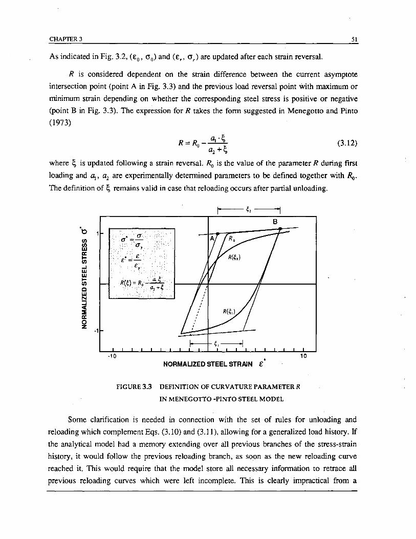
CHAPTER 3 51
As indicated in Fig. 3.2, (Eo, 0'0) and (E" 0',) are updated after each strain reversal.
R is considered dependent on the strain difference between the current asymptote
intersection point (point A in Fig. 3.3) and the previous load reversal point with maximum or
minimum strain depending on whether the corresponding steel stress is positive or negative
(point B in Fig. 3.3). The expression for R takes the form suggested in Menegotto and Pinto
(1973)
R=Ro-~ £lz + ~
(3.12)
where ~ is updated following a strain reversal. Ro is the value of the parameter R during fIrSt
loading and ~, £lz are experimentally determined parameters to be defined together with Ro. The definition of ~ remains valid in case that reloading occurs after partial unloading.
.~
rn rn w a: t; ...J W W t; C W N ::J oct :::IE a: o z
B
• NORMAUZED STEEL STRAIN €
FIGURE 3.3 DEFINITION OF CURVATURE PARAMETERR
IN MENEGOTTO -PINTO STEEL MODEL
Some clarification is needed in connection with the set of rules for unloading and
reloading which complement Eqs. (3.10) and (3.11), allowing for a generalized load history. If
the analytical model had a memory extending over all previous branches of the stress-strain
history, it would follow the previous reloading branch, as soon as the new reloading curve
reached it. This would require that the model store all necessary information to retrace all
previous reloading curves which were left incomplete. This is clearly impractical from a
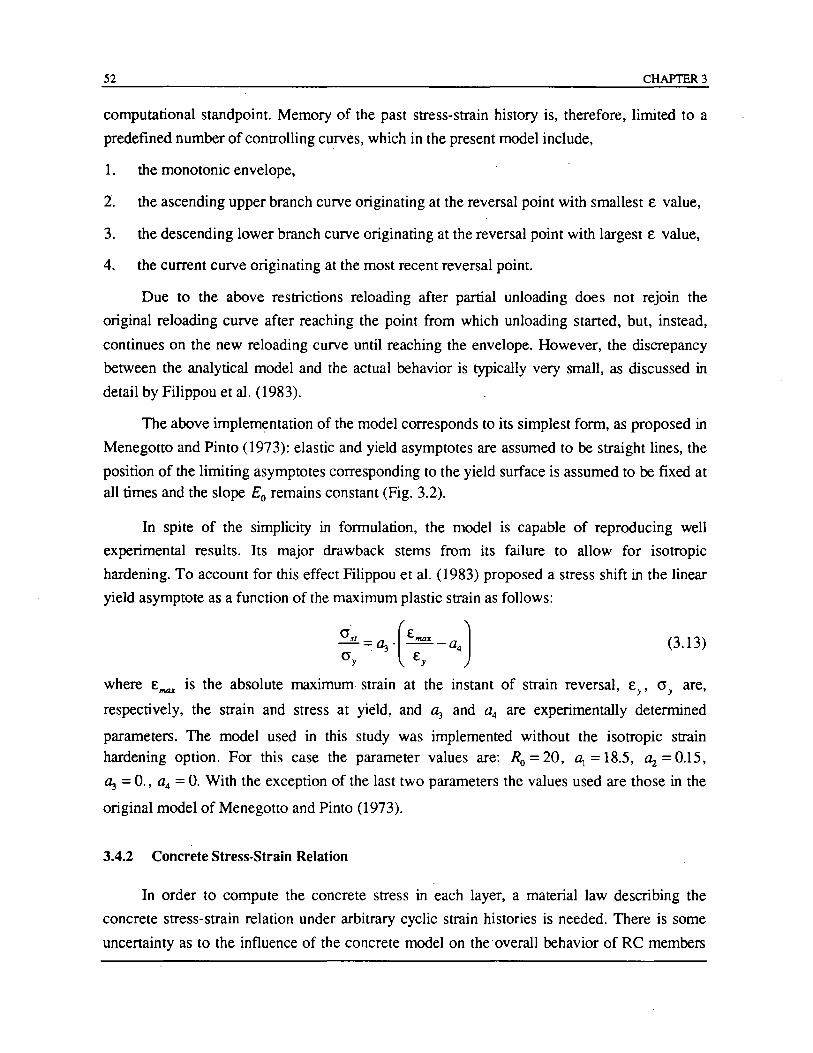
52 CHAPTER 3
computational standpoint. Memory of the past stress-strain history is, therefore, limited to a
predefined number of controlling curves, which in the present model include,
1. the monotonic envelope,
2. the ascending upper branch curve originating at the reversal point with smallest E value,
3. the descending lower branch curve originating at the reversal point with largest E value,
4. the current curve originating at the most recent reversal point.
Due to the above restrictions reloading after partial unloading does not reJOIn the
original reloading curve after reaching the point from which unloading started, but, instead,
continues on the new reloading curve until reaching the envelope. However, the discrepancy
between the analytical model and the actual behavior is typically very small, as discussed in
detail by Filippou et al. (1983).
The above implementation of the model corresponds to its simplest form, as proposed in
Menegotto and Pinto (1973): elastic and yield asymptotes are assumed to be straight lines, the
position of the limiting asymptotes corresponding to the yield surface is assumed to be fixed at all times and the slope Eo remains constant (Fig. 3.2).
In spite of the simplicity in formulation, the model is capable of reproducing well
experimental results. Its major drawback stems from its failure to allow for isotropic
hardening. To account for this effect Filippou et al. (1983) proposed a stress shift in the linear
yield asymptote as a function of the maximum plastic strain as follows:
O"SI = ~ . (Emax - Q4J O"y Ey
(3.13)
where Emaz is the absolute maximum strain at the instant of strain reversal, Ey , 0" yare,
respectively, the strain and stress at yield, and ~ and Q4 are experimentally determined
parameters. The model used in this study was implemented without the isotropic strain hardening option. For this case the parameter values are: Ro = 20, ~ = 18.5, ~ = 0.15,
~ = 0., Q4 = O. With the exception of the last two parameters the values used are those in the
original model of Menegotto and Pinto (1973).
3.4.2 Concrete Stress-Strain Relation
In order to compute the concrete stress in each layer, a material law describing the
concrete stress-strain relation under arbitrary cyclic strain histories is needed. There is some
uncenainty as to the influence of the concrete model on the overall behavior of RC members
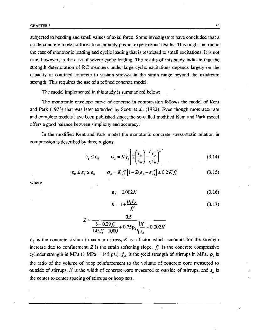
CHAPTER 3 53
subjected to bending and small values of axial force. Some investigators have concluded that a
crude concrete model suffices to accurately predict experimental results. This might be true in
the case of monotonic loading and cyclic loading that is restricted to small excitations. It is not
true, however, in the case of severe cyclic loading. The results of this study indicate that the
strength deterioration of RC members under large cyclic excitations depends largely on the
capacity of confined concrete to sustain stresses in the strain range beyond the maximum
strength. This requires the use of a refined concrete model.
The model implemented in this study is summarized below:
The monotonic envelope curve of concrete in compression follows the model of Kent
and Park (1973) that was later extended by Scott et al. (1982). Even though more accurate
and complete models have been published since" the so-called modified Kent and Park model
offers a good balance between simplicity and accuracy.'
In the modified Kent and Park model ~he monotonic concrete stress-strain relation in
compression is described by three regions:
where
Eo =0.OO2K
K=1+ P.!y/t
I: Z= 0.5
3 + 0.291: + 0.75 fK - 0.OO2K 1451: -1000 Psv--;;:
(3.14)
(3.15)
(3.16)
(3.17)
eo is the concrete strain at maximum stress, K is a factor which -accounts for the strength
increase due to confinement, Z is the strain softening slope, £' is the concrete compressive
cylinder strength in MPa (1 MPa = ,145 psi), ~/t is the yield strength of stirrups in MPa, Ps is
the ratio of the volume of hoop reinforcement to the volume of concrete core measured to
outside of stirrups, h' is the width of concrete core measured to outside of stirrups, and Sh is
the center to center spacing of stirrups or hoop sets.
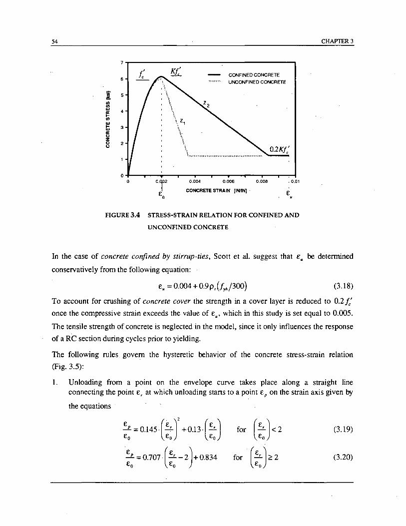
54
i VI VI w a: ..... VI W ..... w a: u z 8
7
6 t: 5
4
3 ,
2
~.
CONFINED CONCRETE
UNCONFINED CONCRETE
\ \. ~\ ......... , ...... w., .......... w ... ".'w ....... ' '''' .... , .... , .• , .... , ................ ,' 0.2 K fe'
o~--~--~--~--~--~~~~~~--~--~, o 0.004 0.006 0.008 ,0.01
CONCRETE STRAIN [INIIN]' E
FIGURE 3.4 STRESS-STRAIN RELATION FOR CONFINED AND
UNCONFINED CONCRETE
CHAP1ER 3
In the case of concrete confined by stirrup-ties, Scott et al. suggest that E .. be determined
conservatively from the following equation:
(3.18)
To account for crushing of concrete cover the strength in a cover layer is reduced to 0.2 f: once the compressive strain exceeds the value of E~, which in this study is set equal to 0.005. The tensile strength of concrete is neglected in the model, since it only influences the response
of a RC section during cycles prior to yielding.
The following rules govern the hysteretic behavior of the concrete stress-strain relation
(Fig. 3.5):
1. Unloading from a point on the envelope curve takes place along a straight line connecting the point Er at which unloading starts to a point Ep on the strain axis given by
the equations
Ep =0.145.(Er J2 +0.13.(~J Eo Eo Eo
2 = 0.707· (~- 2J+ 0.834 Eo Eo
for (:}2 for· (:}2
(3.19)
(3.20)
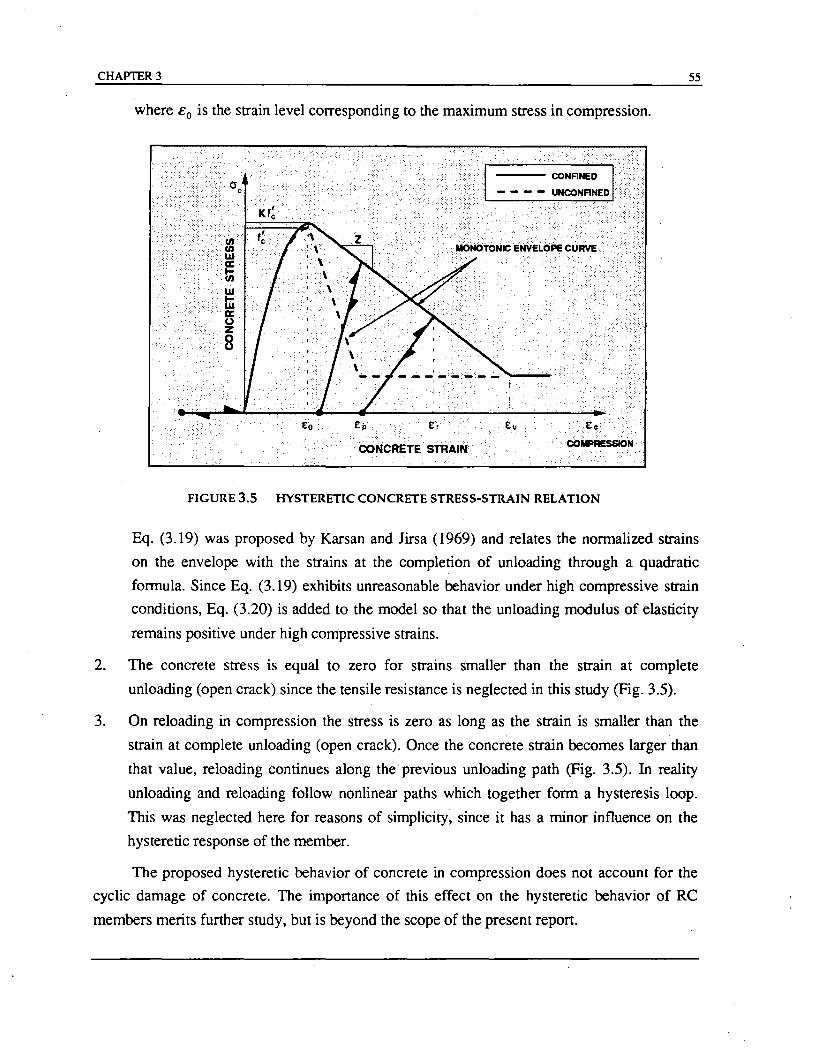
CHAPTER 3 55
where Co is the strain level corresponding to the maximum stress in compression.
FIGURE 3.5 HYSTERETIC CONCRETE STRESS-STRAIN RELATION
Eq. (3.19) was proposed by Karsan and Jirsa (1969) and relates the normalized strains
on the envelope with the strains at the completion of unloading through a quadratic
formula. Since Eq. (3.19) exhibits unreasonable behavior under high compressive strain
conditions, Eq. (3.20) is added to the model so that the unloading modulus of elasticity
remains positive under high compressive strains.
2. The concrete stress is equal to zero for strains smaller than the strain at complete
unloading (open crack) since the tensile resistance is neglected in this study (Fig. 3.5).
3. On reloading in compression the stress is zero as long as the strain is smaller than the
strain at complete unloading (open crack). Once the concrete strain becomes larger than
that value, reloading continues along the previous unloading path (Fig. 3.5). In reality
unloading and reloading follow nonlinear paths which together form a hysteresis loop.
This was neglected here for reasons of simplicity, since it has a minor influence on the
hysteretic response of the member.
The proposed hysteretic behavior of concrete in compression does not account for the
cyclic damage of concrete. The importance of this effect on the hysteretic behavior of RC
members merits further study, but is beyond the scope of the present report.
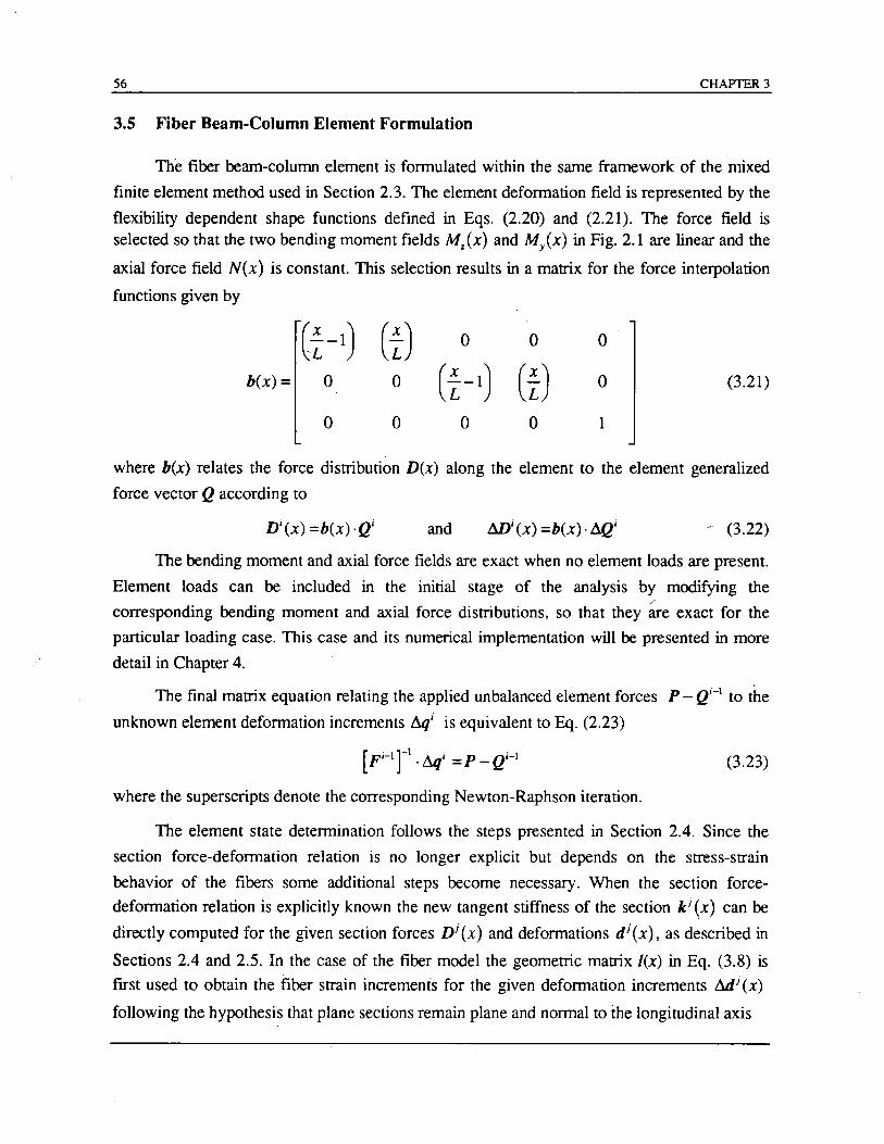
56 CHAPTER 3
3.5 Fiber Beam-Column Element Formulation
The fiber beam-column element is formulated within the same framework of the mixed
finite element method used in Section 2.3. The element deformation field is represented by the
flexibility dependent shape functions defined in Eqs. (2.20) and (2.21). The force field is selected so that the two bending moment fields Mz(x) and My{x) in Fig. 2.1 are linear and the
axial force field N(x) is constant. This selection results in a matrix for the force interpolation
functions given by
(~ -1) (~) 0 0 0
b(x) = 0 0 (~ -1) (~) 0 (3.21)
0 0 0 0 1
where b(x) relates the force distribution D(x) along the element to the element generalized
force vector Q according to
and Mi(x) =b(x). ~Qi - (3.22)
The bending moment and axial force fields are exact when no element loads are present.
. Element loads can be included in the initial stage of the analysis by modifying the
corresponding bending moment and axial force distributions, so that they are exact for the
particular loading case. This case and its numerical implementation will be presented in more
detail in Chapter 4.
The final matrix equation relating the applied unbalanced element forces P - Qi-l to the
unknown element deformation increments Ilqi is equivalent to Eq. (2.23)
(3.23)
where the superscripts denote the corresponding Newton-Raphson iteration.
The element state determination follows the steps presented in Section 2.4. Since the
section force-deformation relation is no longer explicit but depends on the stress-strain
behavior of the fibers some additional steps become necessary. When the section force
deformation relation is explicitly known the new tangent stiffness of the section k j (x) can be
directly computed for the given section forces Dj (x) and defonnations d j (x), as described in
Sections 2.4 and 2.5. In the case of the fiber model the geometric matrix l(x) in Eq. (3.8) is
first used to obtain the fiber strain increments for the given deformation increments Mj (x)
following the hypothesis that plane sections remain plane and normal to the longitudinal axis

CHAPTER 3 57
l!.£j (x)= l(x)' Adj (X)
The fiber strains are then updated to the new value
ej(x)= ej-1(x)+l!.£j(x)
The new stress (J'~b and tangent modulus E~b of all fibers are determined from the
appropriate fiber stress-strain relation: the fiber stresses are then grouped in vector Ej and the tangent moduli are written in a diagonal matrix E~,.. By calling A a diagonal matrix with
entries the areas Ai/ib of all fibers and using the section compatibility matrix l(x) of Eq. (3.8)
well established structural analysis concepts yield the new section tangent stiffness matrix
which after carrying out the multiplication results in
,.(~)
- L Eftu, . Ai/ib . Yifib ifib=l ,.(x)
L E~b . Ai/ib . zijib
i/ib=l ,,( .. ) LE~'~b
i/ib=l
(3.24)
The new ,section tangent stiffness matrix k j (x) is then inverted to obtain the new section
tangent flexibility matrix f' (x). Similarly, the section' resisting forces Dk(x) cannot be
obtained directly from the section force-deformation relation as in Chapter 2, but are
determined by summation of the axial force and biaxial bending contribution of all fibers as
follows
(3.25)
or, after carrying out the multiplications
" - L(J'~b . ~b . Yi/ib
i/ib=l ,. Dk (x) = L (J'~b . Ai/ib . Zi/ib
iJib=l
" L (J' ~b • Aifib ifib=1
It is important to point out that all section matrices and vectors are computed with
respect to a fixed section reference system which coincides with element axes y and z. This
choice simplifies the computational effort. The origin of this reference system (x,O,O), shown
in Fig. 2.1, does not necessarily have to coincide with the neutral axis of the section. Since the
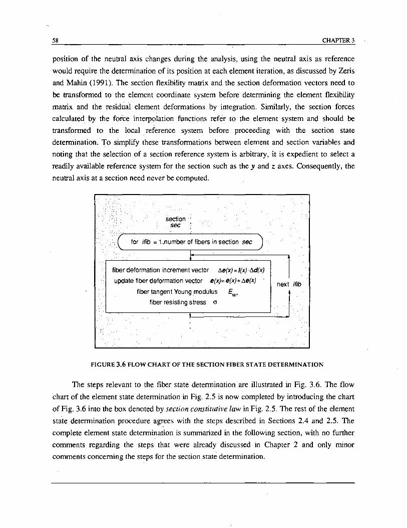
58 CHAPTER 3
position of the neutral axis changes during the analysis, using the neutral axis as reference
would require the determination of its position at each element iteration, as discussed by Zeris
and Mahin (1991). The section flexibility matrix and the section deformation vectors need to
be transformed to the element coordinate system before determining the element flexibility
matrix and the residual element deformations by integration. Similarly, the section forces
calculated by the force interpolation functions refer to the element system and should be
transformed to the local. reference system before proceeding with· the section state
determination.· To simplify these transformations between element and section variables and
noting that the selection of a section reference system is arbitrary, it is expedient to select a
readily available reference system for the section such as the y and z axes. Consequently, the
neutral axis at a section need never be computed.
.
section ' sec
.( for ifib = 1 ,number of fibers in section sec
... . .. fiber deformation increment vector tle(x) = I(x) ·tld(x)
update fiber deformation vector e(x)= e(x) + tle(x)
fiber tangent Young modulus Elan
fiber reSisting stress 0
I
next/fib
FIGURE 3.6 FLOW CHART OF THE SECTION FIBER STATE DETERMINATION
The steps relevant to the fiber state determination are illustrated in Fig. 3.6. The flow
chart of the element state determination in Fig. 2.5 is now completed by introducing the chart
of Fig. 3.6 into the box denoted by section constitutive law in Fig. 2.5. The rest of the element
state determination procedure agrees with the steps described in Sections 2.4 and 2.5. The
complete element state determination is summarized in the following section, with no further
comments regarding the steps that were already discussed in Chapter 2 and only minor
comments concerning the steps for the section state determination.
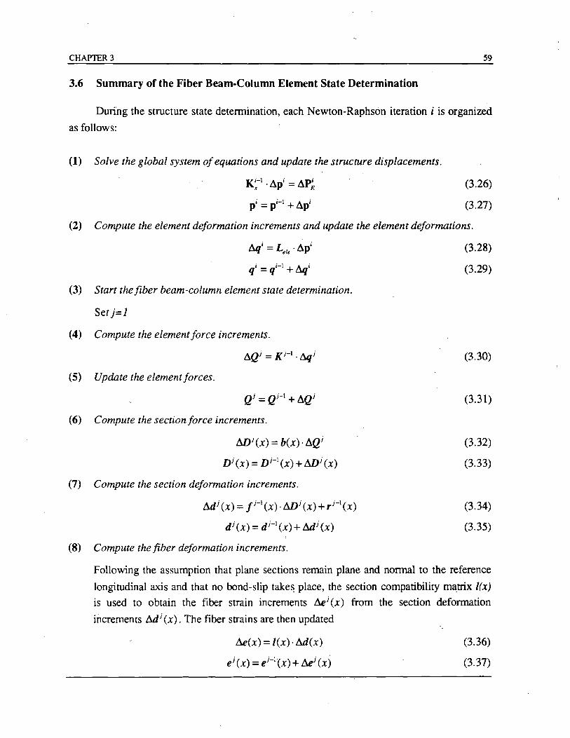
CHAPTER 3 59
3.6 Summary of the Fiber Beam-Column Element State Determination
During the structure state determination, each Newton-Raphson iteration i is organized
as follows:
(1) Solve the global system of equations and update the structure displacements.
(3.26)
(3.27)
(2) Compute the element deformation increments and update the element deformations.
6qi = Lei • . .1.pi
qi = qi-I + Ilqi
(3) Start the fiber beam-column element state determination.
Set)=]
(4) Compute the element force increments .
.1.Qj = K j-I . 6qj
(5) Update the element forces.
(6) Compute the section force increments.
m j (x) = h(x)· .1.Qj
n j (x) = n j
-I (x) + m j (x)
(7) Compute the section deformation increments.
Mj (x) = jj-I (x)· m j (x) + rj-I(x)
d j (x) = d j- I (x) + Mj (x)
(8) Compute the fiber deformation increments.
(3.28)
(3.29)
(3.30)
(3.31)
(3.32)
(3.33)
(3.34)
(3.35)
Following the assumption that plane sections remain plane and normal to the reference
longitudinal axis and that no bond-slip take~ place, the section compatibility matrix l(x)
is used to obtain the fiber strain increments Il£j (x) from the section deformation
increments Mj (x). The fiber strains are then updated
.1.e(x) = l(x)· M(x)
e j (x) = ej-I(x) +.1,ej (x)
(3.36)
(3.37)
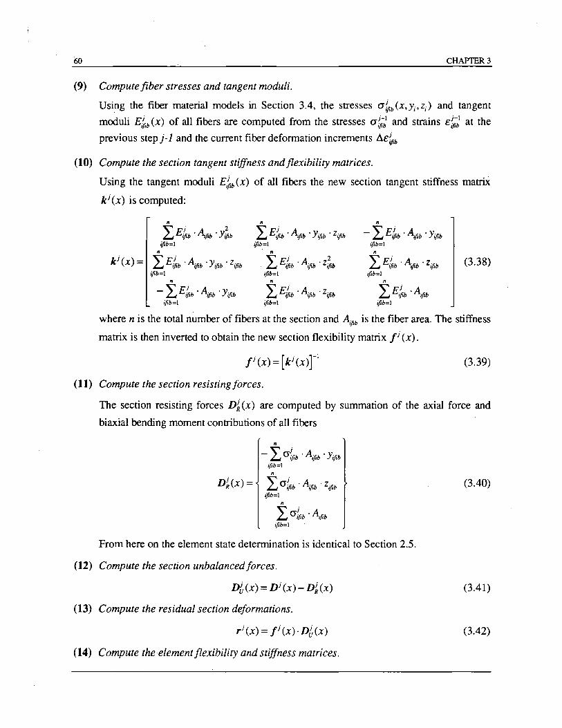
(9) Computejiber stresses and tangent moduli.
Using the fiber material models in Section 3.4, the stresses a~b (x'Yj' Zj) and tangent
moduli E~b (x) of all fibers are computed from the stresses a~~ and strains £~-~ at the
previous step j-l and the current fiber deformation increments Ll£~b
(10) Compute the section tangent stiffness and flexibility matrices.
Using the tangent moduli E~b(X) of all fibers the new section tangent stiffness matrix
k i (x) is computed:
11 11 11
L i 2 EiJib . A;Jib . YiJib L E~b . A;Jib . YiJib . ZiJib - LE~b' Aq;b' YiJib iJib=! iJib=1 jJib=1
11 11 11
k i (x) = LE~b ·AiJib 'YiJib 'ZiJib L i 2 . EiJib . A jJib . ZiJib LE~b ·AiJib 'ZiJib (3.38) iJib=! iJib=1 jJib=1
11 11 11
- LE~b ·AiJib 'YiJib L E~b . AiJib . ZjJib L E/fib . A jJib iJib=! jJib=! iJib=!
where n is the total number of fibers at the section and A jJib is the fiber area. The stiffness
matrix is then inverted to obtain the new section flexibility matrix ji (x).
(3.39)
(11) Compute the section resisting forces.
The section resisting forces D~(x) are computed by summation of the axial force and
biaxial bending moment contributions of all fibers
11
- L (J~b . AiJib . Y iJib iJib=1
11
D~(x) = L (J~b . A jJib . ZiJib iJib=1
11
L (J~b . A jJib iJib=1
From here on the element state determination is identical to Section 2.5.
(12) Compute the section unbalancedforces.
D{(x) = Di (x) - D~(x)
(13) Compute the residual section deformations.
ri (x) = ji (x)· D{(x)
(14) Compute the element flexibility and stiffness matrices.
(3.40)
(3.41)
(3.42)
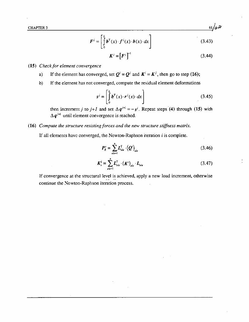
CHAPTER 3 61J~,:Jj ~~~~----------------------------------------------------------~.
FI ~ [l bT(X).jl(X).b(X)'dx]
Ki=[Fir (15) Checkfor element convergence
a) If the element has converged, set Qi = Qj and Ki = K j , then go to step (16);
b) If the element has not converged, compute the residual element deformations
Sl ~ [1 bT (x).rl(X)'dx]
(3.43)
(3.44)
(3.45)
then increment j to j+ 1 and set D. qj+! = - sj. Repeat steps· (4) through (15) with
D. qj+! until element convergence is reached.
(16) Compute the structure resisting forces and the new structure stiffness matrix.
If all elements have converged, the Newton-Raphson iteration i is complete.
n
p~ = LL:le . (Qlle (3,46) ele=!
n
K; = LL:le . (Ki)ele ·Lele (3.47) ele=!
If convergence at the structural level is achieved, apply a new load increment, otherwise
continue the Newton-Raphson iteration process.

CHAPTER 4
NUMERICAL IMPLEMENTATION OF BEAM-COLUMN ELEMENT
4.1 General
A discussion of some of the issues involved in the numerical implementation of the fiber.
beam-column element in a general purpose computer program is presented in this chapter. The
element was first implemented in a stand-alone computer program. After successfully testing
its performance, the element was adapted to the finite element program FEAP developed by
Professor R. L. Taylor at the University of California, Berkeley and described in Zienkiewicz
and Taylor (1989 and 1991). The present report focuses on the numerical aspects of the stand
alone program and briefly discusses some differences in the numerical strategies between the
stand alone program and the implementation in FEAP.
The stand-alone program is a special purpose program for the analysis of frames
composed of fiber beam-column elements. The input data contain information concerning the
geometry and material properties of the structure as well as information about the applied
loads, which include both nodal and element loads. Nodal loads can be constant or time
varying, in which case they are applied in a sequence of steps. Element loads are constant and
are applied with the constant nodal loads at the beginning of the analysis.
The nonlinear solution algorithm is divided into three nested loops. The first and'
outermost loop consists of the sequence of load steps that the applied load is divided into. The
second loop consists of the Newton-Raphson solution procedure that is necessary within each
load step for determining the structural displacements that result from the total applied load.
This loop is also referred to as structure state determination. The third and innermost loop
consists of the element iteration process that is necessary within each Newton-Raphson
iteration in order to compute the element resisting forces that correspond to given element
deformations. This loop is also referred to as element state determination.
In order to better illustrate the three nested loops the notation in the previous chapters is
extended so that every variable now carries information about the load step number, the
current Newton-Raphson iteration and, when necessary, the current element iteration. This
information is represented by three different superscripts on the variable: consistent with the
63
64 CHAPTER 4
notation in the two previous chapters, k refers to the load step, i to the Newton-Raphson
iteration scheme and j to the element iteration loop. This notation is particularly useful in the
numerical implementation of the nonlinear solution algorithm, which is summarized in
Appendix A.
After a brief discussion of the notation and the numerical scheme for the integration
along the element axis, the problem of defining a convergence criterion, both, at the element
and at the structure level is discussed. Different alternatives are explored outlining their
advantages and disadvantages. The criteria used in the stand-alone program are based on
unbalanced forces, both, at the structure and at the element level, while program FEAP uses
an energy criterion at the structure level, so that a corresponding criterion is adopted at the
element level.
The procedure for including element loads in the model is presented next. An initial
force distribution that is in equilibrium with the applied element loads is assumed first. The
corresponding residual element deformations are used to start the element iterations that will
ultimately yield the fixed-end moments for the applied element loads. Rigid body modes are
then added in order to include the shear forces due to the element loads. The resulting end
moments and shear forces do not generally satisfy equilibrium at the structural nodes, because
no nodal forces were originally applied to the structure in connection with the element loads.
The resulting end moments and shear forces contribute to the unbalanced nodal loads that
need to be applied with opposite sign at the structural nodes in order to restore equilibrium.
This step concludes the first Newton-Raphson iteration for the element load application. If the
element is elastic, no further iterations are required within the element and the resulting end
moments constitute the fixed-end moments for the applied element loads. If the element
undergoes inelastic behavior under the application of element loads, the iterations of the
element state determination phase of the algorithm converge to the fixed-end forces of the
elemeilt.
Two alternative methods for including the shear forces are presented. One is
implemented in the stand alone program and the other is used in program FEAP. A simple
example of a linear elastic cantilever with uniformly distributed load is used to illustrate the
process of element load application.
A brief discussion of the application of the nonlinear algorithm to the state
determination of softening elements concludes the chapter. A simple system of two springs in
series is used to illustrate how well the proposed algorithm works for softening elements.
CHAPTER 4 65
4.2 Preliminary Considerations
The implementation of the fiber beam-column element evolved over two stages. A stand
alone computer program was developed fITst in order to test the element performance. In the
second stage the element was implemented in the finite element program FEAP. In this report
the computational considerations concerning the general implementation of the element rather
than the specific details for the two numerical implementations are discussed.
In both implementations the input data consist of the geometry description and material
properties of the structure. From the geometric viewpoint the structure is an assemblage of
beam-column elements connected at nodes so that the nodal degrees of freedom, grouped in
vector p, are the basic unknowns of the problem. The element deformations q are related to the structure degrees of freedom p through a constant compatibility matrix Lde • Each element
is subdivided into several control sections and each section is composed of a number of fibers.
The number of sections and their locations depends on the integration scheme and the desired
level of accuracy. The number of fibers in a section depends on the geometric and material
properties of the section and on the level of detail sought in the section representation. Each
fiber is characterized by its area, material type and position with respect to the section
reference system (Fig. 3.1). The origin of this local system is the-geometric centroid of the
section. The union of the geometric centroids of the section defines the longitudinal axis of the
element x. The material behavior of the element depends entirely on the fiber stress-strain
relation of the fibers, which follow the confined and unconfined concrete as well as reinforcing
steel models of Section 3.4. Different concrete and steel material types can be specified for the
fibers by varying the values of material parameters.
External loads can be applied to the structure in the form of nodal forces or element
loads. Incremental static loads can be included in the analysis with the introduction of a
fictitious time scale. In general, all constant loads are applied at the beginning of the analysis,
while incremental loads are applied in a sequence of steps k=l , ... , nk. Two different methods c
are used for the application of nodal forces and element loads. Following classical structural
analysis methods nodal loads are assembled in the global force vector PE • Element loads are
included in an element load vector Wand a new method for incorporating these loads within a
flexibility-based beam element is described in Section 4.5.
The nonlinear analysis algorithm is organized in four modules corresponding to the
different discretization levels of the structure. The four modules refer to structure, elements,
sections and fibers. The vectors and matrices that represent the basic variables within each
module are summarized in Table 4.1.
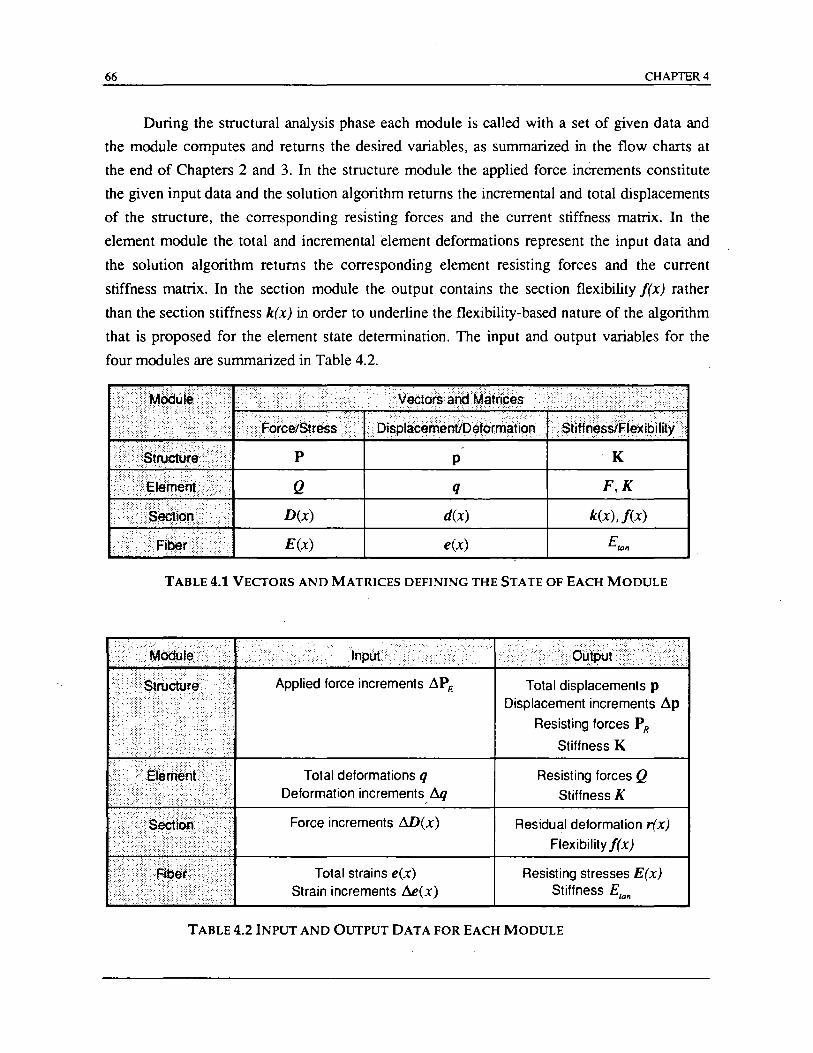
66 CHAPlER4
During the structural analysis phase each module is called with a set of given data and
the module computes and returns the desired variables, as summarized in the flow charts at
the end of Chapters 2 and 3. In the structure module the applied force increments constitute
the given input data and the solution algorithm returns the incremental and total displacements
of the structure, the corresponding resisting forces and the current stiffness matrix. In the
element module the total and incremental element deformations represent the input data and
the solution algorithm returns the corresponding element resisting forces and the current
stiffness matrix. In the section module the output contains the section flexibility f(xJ rather
than the section stiffness k(x) in order to underline -the flexibility-based nature of the algorithm
that is proposed for the element state determination. The input and output variables for the
four modules are summarized in Table 4.2.
P p cK
Q q F,K
D(x) d(x) k(x), f(x)
E(x) e(x) E/Q1I
TABLE 4.1 VECTORS AND MATRICES DEFINING THE STATE OF EACH MODULE
Total deformations q Deformation increments, Ilq
Force increments W(x)
Total strains e(x) Strain increments &>(x)
Total displacements p Displacement increments ~p
Resisting forces PR
Stiffness K
Resisting forces Q Stiffness K
Residual deformation r(x)
Flexibility f(xJ
Resisting stresses E(x) Stiffness E,oll
TABLE 4.2 INPUT AND OUTPUT DATA FOR EACH MODULE
CHAPTER 4 67
The .nonlinear solution algorithm is organized in three nested computational loops.
Loads are applied in a sequence of load steps, that are indicated by superscript k, so that each
load increment is denoted by vector .6.P;. The total applied load PEis equal to the sum of load
increments .6.P;, i.e.
Because of nonlinear structural behavior, a linearization is introduced about the present state
of the structure and an iteration scheme is needed to compute the structure displacements pol:
that result from the imposed forces pol: = p.I:-l + .6.p.I: at each load step. To this end the
Newton-Raphson algorithm is used in the stand alone computer program and in program
FEAP, even though alternative strategies are available in the latter and can be implemented
easily. Another index i is introduced for the iterations of the Newton-Raphson solution
method. Finally, a third iteration loop is needed within each Newton-Raphson iteration in
order to determine the element resisting forces for the given element defonnations qi.
Correspondingly, a third superscriptj is introduced.
From this discussion it is clear that two nested loops are needed within each load step k
in order to obtain a converge<;i solution at the struct,ure degrees of freedom. The solution
algorithm is such that, at the converged state, equilibrium and compatibility are strictly
satisfied within the elements, while all section states satisfy the section force-deformation
relation within the specified tolerance.
A special notation is introduced to trace the evolution of each variable during the
nonlinear analysis. Vectors and matrices are denoted by three superscripts corresponding to
the three iteration loops. For example, the notation for the element force vector Q is
where k indicates the load step, i the Newton-Raphson iteration and j the element iteration. It
should be pointed out that element, section and fiber variables carry all three superscripts,
whereas structure variables do not carry the superscript j, since they do not change during
element iterations. For example, the structure displacement vector and the element force
vector are written
The only exception to this rule is the element deformation vector q, which does not carry the
index j because it is not affected by the element iteration loop (Fig. 2.5).
68 CHAPTER 4
The numerical implementation of the beam-column element in a finite element program
follows very closely the procedure outlined in Chapters 2 and 3. In addition, it requires the
introduction of an incremental vector for each vector that varies during the iterations. For
instance, (Mpl r is the change in the structural displacement increments at the i-th Newton-
Raphson iteration, whereas (~pk)i -denotes the total structural displacement increment during
the k-th load step, which is updated using
(~plr = (~pkrl +(8~pkr
where (~pk y=o = O. Once convergence is reached at the structure degrees of freedom, the
superscript i is dropped and the total displacement increments simply become ~pk, while the
total structural displacements are updated to the value
pk = pk-l + ~pk _
Similarly, (( MQkni
is the change in the element force increments m the j-th element
iteration, and ((~QkrY is the total element force increment during the i-th Newton-Raphson
iteration, which is updated using
((~Qkrr = ((~Qkrrl +((8~Qkrr
where (( ~Qk r f = ( .1Qk r 1 and (( ~Qk n° = O. When convergence is reached in the element
iterations, the superscript j is dropped and (( ~Qk r r becomes (~Qk r. Similarly, when
convergence is also reached at the structure degrees of freedom, superscript i is dropped and
(.1Qk Y becomes .1Qk. At this point the element forces are updated using
with QO = o.
It should be noted that, the change in vector increments, denoted by symbol 8~, is only
used to update the corresponding vector increments and total vectors during the iterations,
and, therefore, does not need to be stored.
The summary of the nonlinear solution algorithm was already presented at the end of
Chapters 2 and 3 with a notation that did not use all superscripts for the sake of clarity.
Appendix A contains a more detailed summary of the solution algorithm with an outline of the
updating procedure and a brief discussion of some implementation issues.
CHAPTER 4 69
4.3 Numerical Integration
All integrals in the element formulation are evaluated numerically with the Gauss-Lobato
integration scheme that is based on the expression L m
1= J !(x)·dx = L wh • !(x/.) (4.1) o h=l
whereh denotes the monitored section and wh is the corresponding weight factor. The Gauss-
Lobato scheme with m integration points permits the exact integration of polynomials of
degree up to (2m-3). This procedure is superior to the classical Gauss integration method,
when it is important to include m the integration the end points of the element. Since inelastic
behavior in beam-column elements often concentrates at the ends of the member, the
monitoring of the end sections of the element offers advantages from the standpoint of
accuracy and numerical stability.
4.4 Definition of Tolerance
The nonlinear solution algorithm in this study is based on a set of linear matrix relations
that are repeatedly applied until convergence is achieved. Theoretically, this occurs when the
applied loads are perfectly balanced by the internal resisting forces of the elements.
Numerically, however, such perfect balance is either impossible or too expensiv~ to attain. In
a nonlinear solution algorithm it is normally accepted that convergence is reached when some
control parameters, such as the unbalanced forces, are smaller than a specified threshold or
tolerance. Norms or absolute values of these variables may be selected as control parameters
as many studies to date have discussed. Different control parameters are selected for the stand
alone program than for the implementation of the element in program FEAP, where the choice
of tolerance parameters is limited by the main program.
In the stand-alone program two different iteration algorithms are used: the first is
implemented at the structure level and is the well known Newton-Raphson scheme, while the
second is used at the element level, as described in the previous chapters. Correspondingly,
two convergence controls are needed. In this study the unbalanced forces at the structure
degrees of freedom and at the control sections of the element are selected as control
parameters. Two types of tolerance are defined: the first is an absolute force bound and the
second is a relative force bound defined as a fraction of the corresponding total applied force.
The unbalanced force is compared with the largest of the two bounds. This choice derives
from the consideration that the absolute tolerance is too restrictive for large applied loads,
70 CHAPTER 4
while the relative check may be too severe for small loads. Since the stability of the proposed
solution algorithm is not affected by the size of the load step increments, the selected
convergence criteria are not overly restrictive in the extreme case of very small or very large
load steps. In the following the convergence criteria at the element and at the structure level
are discussed separately.
(a) Element convergence. Convergence at the element level is achieved when all monitored
sections have converged. Section convergence is reached when all section force
unbalances fall within the absolute or relative tolerance. Three generalized forces, two bending moments Dt(xh ), D2 (Xh ) and the axial force D3(Xh ) are defined at each
monitored section h, as shown in Fig. 2.1. Two element tolerance values are defined for
all elements. These are called:
EAT = Element Absolute Tolerance
ERT = Element Relative Tolerance
ERT and EAT are related to the corresponding structure tolerances SRT and SAT
through a scale factor that is selected by the user, as will be discussed later in the section. At every element iterationj three different section tolerance values SeT,,(xh) are defined:
Se7;,(xh) = max { EAT xL, (( D:(xh) rr x ERT} n = 1,2
SeT,. (xh ) = max { EAT, ((D:(Xh)rr x ERT} n = 3
where L is the element length: In the computer program an element counter EC is
introduced to monitor the number of force unbalances that are smaller than the
corresponding tolerance. During the element iterations the counter is first initialized to
zero and is then incremented by one every time a section force satisfies the section
tolerance, i.e.
Element convergence is reached when all monitored sections have converged, or, in
symbols when
EC = 3m => element convergence
where m is the number of monitored sections in the element. At this point iteration loop j
is complete. After all elements converge the element state determination is complete and
CHAPTER 4 71
the program checks for convergence at the structure level.
(b) Structure convergence. Convergence at the structure level is reached when all nodal
unbalanced forces are smaller than the corresponding tolerance. The convergence check
is similar to that adopted for the element. Absolute and relative tolerances are specified
in the input data:
SAT = Structure Absolute Tolerance
SRT = Structure RelativeTolerance
SRT is typically assigned a value of 0.01, while SAT depends on the type of problem to
be solved. For each degree of freedom ndof a tolerance measure is computed
ndof = 1, ... ,maxdof
where maxdof is the total number of unconstrained degrees of freedom. A structure
counter SC is introduced to monitor the number of converged degrees of freedom. This
counter is initialized to zero at the beginning of every Newton-Raphson iteration i and is
incremented by one every time a structure unbalance force is smaller than the
corresponding tolerance, i.e.
(P;ndof r ~ StT ruin! ::::> SC = SC + 1
Structure convergence is reached when the counter is equal to the total number of
unconstrained degrees of freedom, that is:
SC = maxdof ::::> structure convergence
When the structure converges, the Newton-Raphson loop is complete and the next load
increment is applied.
Structure and element tolerances are related by a tolerance factor TF, such that
EAT=TFxSAT
ERT=TFxSRT
The default value for TF is 1. As TF becomes larger, the number of element iterations j
decreases and in the limit tends to 1. Conversely, as TF gets smaller, the number of iterations j
increases. When load increments are small, few Newton-Raphson iterations are needed to
achieve convergence at the structure level, because only small stiffness changes occur within
each load step. There is, therefore, no need to be overly restrictive during the element
72 CHAPTER 4
convergence check and factor TF can be larger than 1 with typical values ranging from 5 to
10. On the other hand, when load increments are large, significant stiffness changes may take
place within a load step and several Newton-Raphson iterations are needed to converge to the
solution. In this case it is important to trace closely the force-deformation relation at the
element level by selecting a TF value close to 1. In other words the TF factor controls the
relation between the number of iterations) within each Newton-Raphson iteration i and the
total number of Newton-Raphson iterations within a load step.
- . The convergence criteria in program FEAP are different. At the structure level the work
(energy) increment is chosen. as the convergence control parameter. Convergence of the
Newton-Raphson iteration algorithm is reached when the ratio between the current work
increment and the initial work increment is smaller than a specified tolerance. With the
adopted notation the structural convergence criterion is:
{[(~p;rr .(O~pky}
{[(~p;Yr .(o~pkr} ~ Stol (4.2)
Typically, Stol is assigned the value of 10-16 by default. This convergence scheme is part of
the FEAP program and is completely independent of the present application. More details on
the convergence criterion can be found in Zienkiewicz and Taylor (1989 and 1991).
In the implementation· of the beam-column element in program FEAP the same
convergence criterion is used to check convergence within the element iteration loop. The
value of the work increment for the current element iteration) is compared to the work for the
first element iteration, i.e. )=1. In symbols:
{[( (MQ' n'T (( Mq' l'Y) {[((MQ'nT(Mq')'}
(4.3)
Typically, Etol is assigned the value of 10-16 by default. This criterion has a clear advantage
over that used in the stand-alone program, since it controls, both, unbalanced forces and
residual deformations. This is quite significant when the element reaches its peak resistance
and its stiffness matrix becomes ill-conditioned. In this case the unbalanced forces may be very
small while the element residual deformations are still large. Consequently, the element
iterations, which are based on residual deformations, should not stop. Energy is the only
measure which accounts for, both, unbalanced forces and residual deformations.

CHAPTER 4 73
Another significant difference between the element convergence criterion in the stand
alone program and that in program FEAP is that in the former case element convergence is
based on section convergence, while· in the latter convergence is entirely based on element
forces and deformations, implicitly assuming that convergence at the element degrees of
freedom implies section convergence. To validate this assumption another convergence
criterion was also introduced in the implementation of the element in FEAP. In this third
criterion convergence is also checked at the section level by measuring the energy increment
rather than the unbalanced forces. In this case convergence is achieved when the following
" condition is satisfied:
I {[ ((r'(x;~lr)'J' . ((k'(x;,Jr)i . ((r'(x;=lr)i}
I {[({Iid'{X;,~ln' r . ((k' (x; = llY . ({Iid'{X;,~Jr)'} :5 Etal (4.4)
In the test phase of the element implementation the convergence criteria in Eqs. (4.3) and
(4.4) proved equally effective. Consequently, the convergence criterion in Eq. (4.3) that is
only based on the energy at the element level is selected in this study, since it leads to shoner
calculation times.
4.5 Application of Element Loads
A new method for the application of element loads in the context of a flexibility based
beam-column element is presented in this section. In the linear elastic range, both, stiffness
and flexibility methods yield identical results, so that well established methods for the
calculation of equivalent nodal forces based on displacement shape functions can be used. In
the nonlinear range, however, different methods need to be used in the two cases. The'method
proposed in this study follows the nonlinear solution algorithm for applied nodal loads. In the
stand-alone program only uniform loads are included in the element. These are applied during
the first load step corresponding to k=l. In program FEAP different element load distributions
can be included.
The application of element loads is more complex than that of nodal loads, since it
requires the explicit inclusion of rigid-body modes. Rigid-body modes have not been
considered so far, because they are not necessary for the element formulation. They are implicitly included in the transfonnation matrix Lele in Eqs. (2.28), (2.43) and (2.44), which
"transforms the element displacements p from the global reference system to the element
74 CHAPTER 4
deformations q in the local reference system. Transverse element loads induce shear forces in
the element that can only be accounted for by the inclusion of rigid-body modes. The effect of
rigid body modes in the application of element loads can be included in different ways. In_ this
section the original implementation in the stand-alone program is described; with a brief
discussion of the method used in program FEAP.
The procedure for the application of element loads consists of the following steps. For
simplicity the structure is assumed to be at an initial unstressed state, with unstressed elements
and sections and no nodal loads present. The bending moment and axial force diagrams that
result from the application of element loads on a statically determinate simply supported beam
are imposed as incremental forces at the sections of the unstressed element without rigid lxxiy
modes. These section forces induce section deformations that are integrated along the element
to yield the corresponding element deformations. The latter violate the compatibility condition
at the structure level that element displacements and deformations be equal to zero for zero
extemalloads. ~orrective forces need to be applied at the member ends to restore the element
deformations to zero, exactly as is the case in the algorithm of the nonlinear element state
determination. For nonlinear element behavior under the applied element loads the iterations
continue within the element until convergence is achieved. Upon convergence the element
resisting forces are computed and the equilibrium is checked at the structure degrees of
freedom. Since no external loads are present, the element resisting forces violate the
equilibrium at the structure degrees of freedom and their nodal equivalents must be applied
with opposite sign to the structure. These nodal forces are, thus, treated as structure
unbalanced loads. From this point on the procedure is identical to the application of nodal
loads. For nonlinear .behavior under the applied element loads Newton-Raphson iterations are
necessary to reach the converged state of the structure. At the end of the initial load step the
bending moment distribution in the elements is not linear, since it results from the
superposition of the generally nonlinear force distribution for the applied element loads with
the linear bending moment distribution due to nodal load corrections. If no nodal loads are
applied to the structure in the fIrst load step, the final state of the structure is one with zero
nodal forces but non-zero nodal displacements due to the applied element loads.
Rigid-body modes are important in the application of element loads. The beam-column
element without rigid-body modes is shown in Fig. 2.1. When the rigid-body modes are
included, five additional degrees of freedom appear, as shown in Fig. 4.1, with the relevant
forces Q and displacements q expressed relative to the local reference axis. The rigid-body
modes are added before checking convergence within the Newton-Raphson iteration i. From
equilibrium considerations Q is first expanded to Q and then the forces at the additional
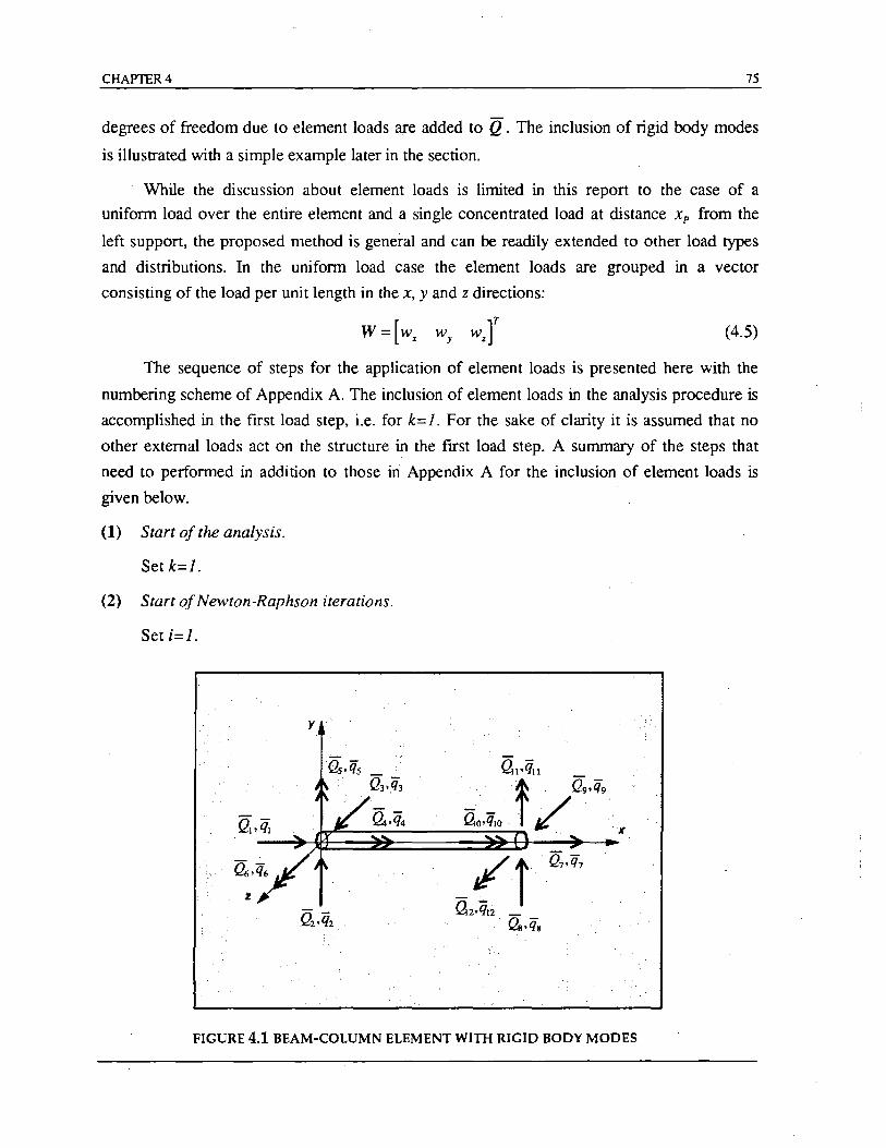
CHAPTER 4 75
degrees of freedom due to element loads are added to Q . The inclusion of rigid body modes
is illustrated with a simple example later in the section.
While the discussion about element loads is limited in this report to the case of a
uniform load over the entire element and a single concentrated load at distance Xp from the
left support, the proposed method is general and can be readily extended to other load types
and distributions. In the uniform load case the element loads are grouped in a vector
consisting of the load per unit length in the x, y and z directions:
(4.5)
The sequence of steps for the application of element loads is presented here with the
numbering scheme of Appendix A. The inclusion of element loads in the analysis procedure is
accomplished in the ftrst load step, i.e. for k=l. For the sake of clarity it is assumed that no
other external loads act on the structure in the ftrst load step. A summary of the steps that
need to performed in addition to those ill Appendix A for the inclusion of element loads is
given below.
(1) Start of the analysis.
Set k=l.
(2) Start of Newton-Raphson iterations.
Set i=l.
y
FIGURE 4.1 BEAM-COLUMN ELEMENT WITH RIGID BODY MODES
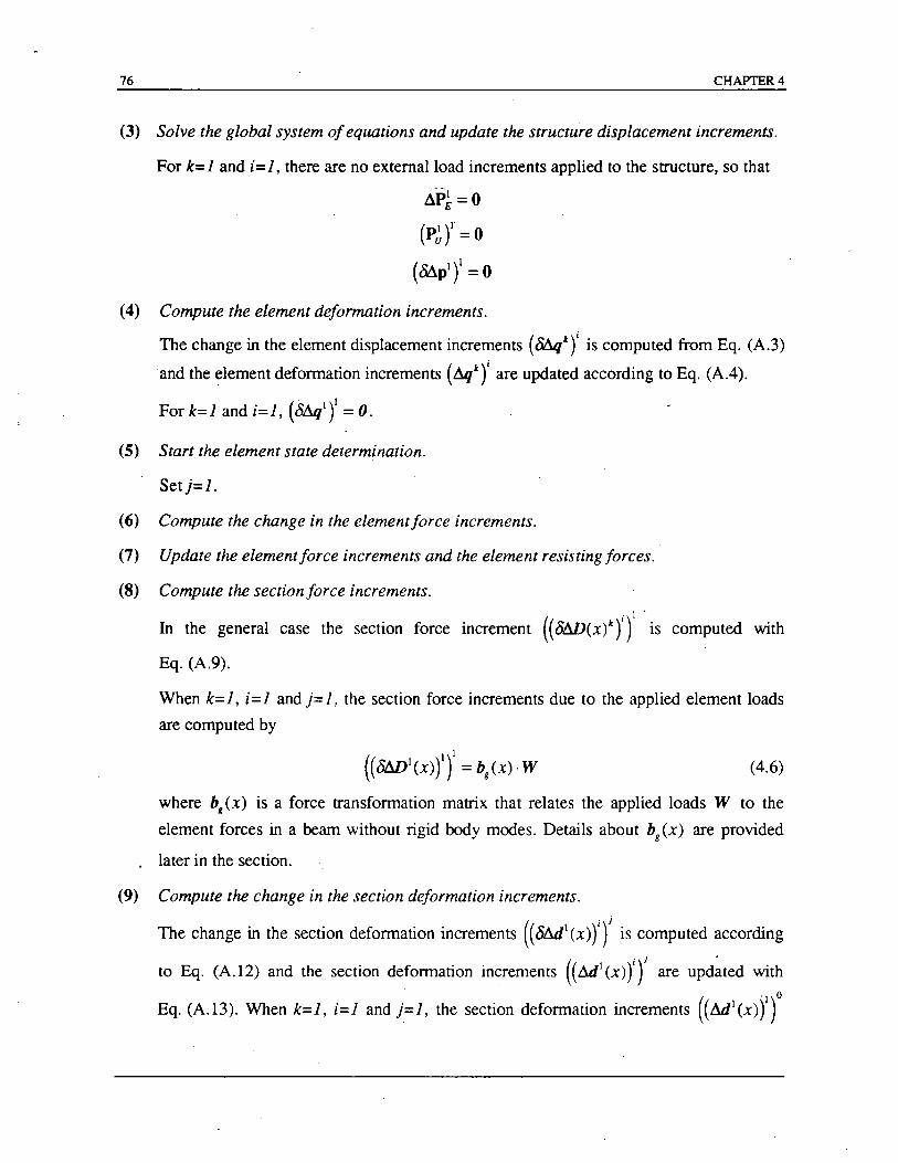
76 CHAPTER 4
(3) Solve the global system of equations and update the structure displacement increments.
For k=1 and i=1, there are no external load increments applied to the structure, so that
ipi=O
(p~r = 0
(8.1plr = 0
(4) Compute the element deformation increments.
The change in the element displacement increments (M.qt)i is computed from Eq. (A.3)
and the element defonnation increments (L\{lr are updated according to Eq. (A.4).
For k=1 and i=1, (M.qI)1 = O.
(5) Start the element state determination.
Set)=1.
(6) Compute the change in the elementforce increments.
(7) Update the elementforce increments and the element resisting forces.
(8) Compute the section force increments. . I .
In the general case the section force increment ((8L\D(X)k)') is computed with
Eq. (A.9).
When k=1, i=1 and )=1! the section force increments due to the applied element loads
are computed. by
(4.6)
where bg(x) is a force transfonnation matrix that relates the applied loads W to the
element forces in a beam without rigid body modes. Details about bg (x) are provided
later in the section.
(9) Compute the change in the section deformation increments.
The change in the section defonnation increments (( 8&t (x) r r is computed according . j •
to Eq. (A.12) and the section defonnation increments (( &t (x»),) are updated with
Eq. (A.l3). When k=1, i=1 and )=1, the section defonnation increments ((&t(X»)'f
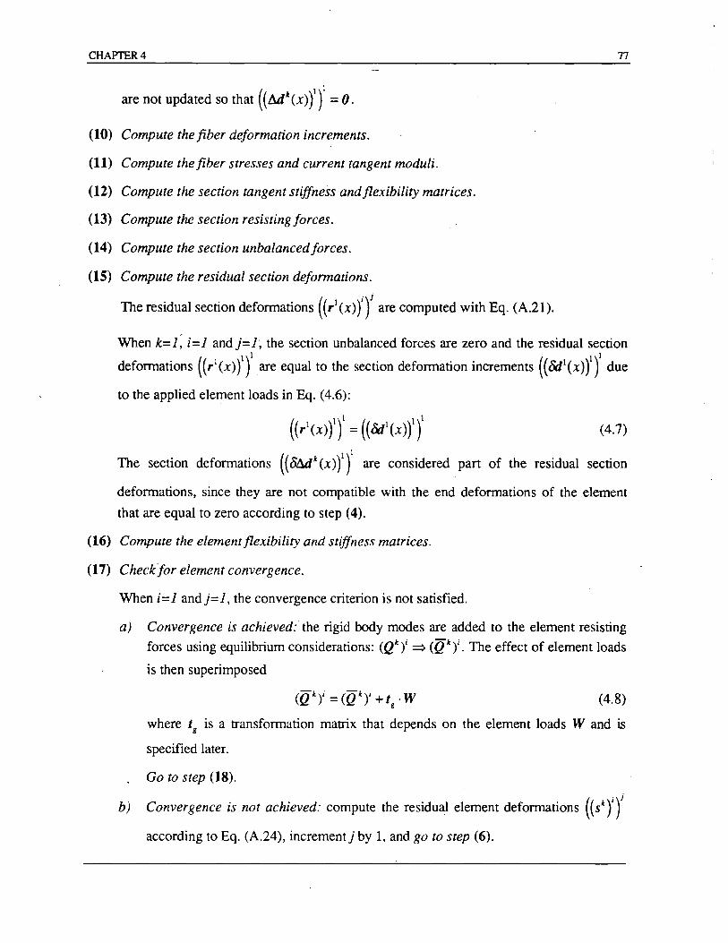
CHAPTER 4
are not updated so that (( .&t (x) n 1 = O.
(10) Compute the fiber deformation increments.
(11) Compute the fiber stresses and current tangent moduli.
(12) Compute the section tangent stiffness andflexibility matrices.
(13) Compute the section resisting forces.
(14) Compute the section unbalancedforces.
(15) Compute the residual section deformations.
The residual section defonnations ((rl(x)Y)J are computed with Eq. (A.21).
77
When k=1, ;=1 and j=1; the section unbalanced forces are zero and the residual section 1 1
deformations ((rl(x)n are equal to the section defonnation increments ((&ll(x)n due
to the applied element loads in Eq. (4.6):
(4.7)
The section defonnations ((Mdt (x) f)1 are considered part of the residual section
deformations, since they are not compatible with the end deformations of the element
that are equal to zero according to step (4).
(16) Compute the element flexibility and stiffness matrices.
(17) Check/or element convergence.
When i = 1 and j= 1 , the convergence criterion is not satisfied.
a) Convergence is achieved:" the rigid body modes are added to the element resisting
forces using equilibrium considerations: (Q"Y ~ (Q"( The effect of element loads
is then superimposed
(4.8)
where tg is a transformation matrix that depends on the element loads Wand is
specified later.
Go to step (18).
b) Convergence is not achieved: compute the residual element deformations ((s"YY according to Eq. (A.24), incrementj by 1, and go to step (6).
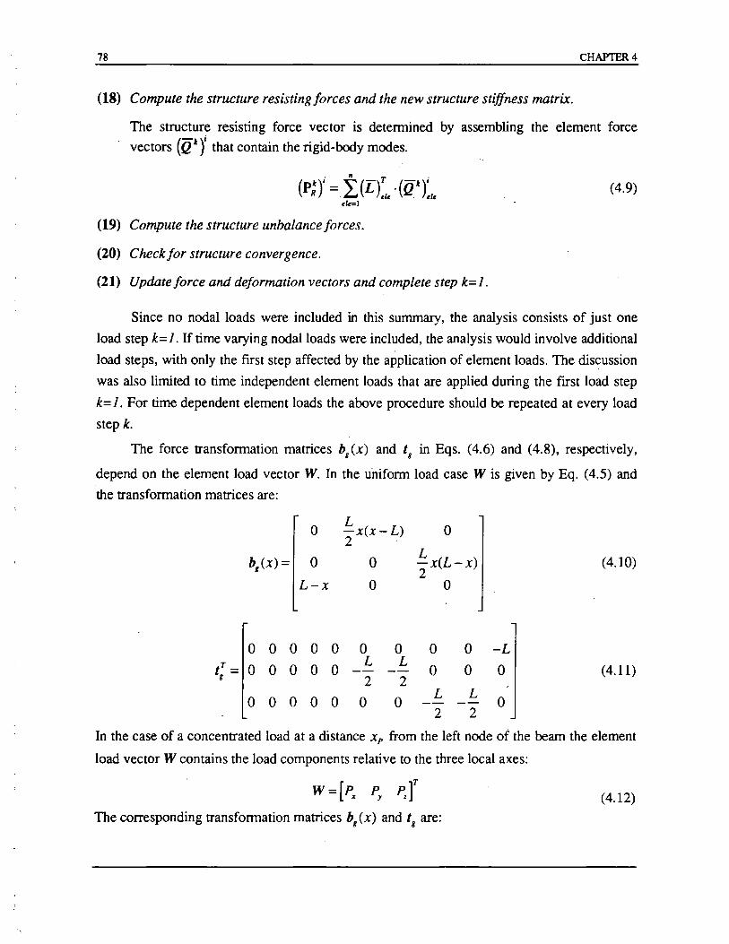
78 CHAPTER 4
(18) Compute the structure resisting forces and the new structure stiffness matrix.
The structure resisting force vector is detennined by assembling the element force
vectors (Q l Y that contain the rigid-body modes.
(19) Compute the structure unbalance/orces.
(20) Check/or structure convergence.
(21) Update force and deformation vectors and complete step k=l.
(4.9)
Since no nodal loads were included in this summary, the analysis consists of just one
load step k=l. If time varying nodal loads were included, the analysis would involve additional
load steps, with only the fIrst step affected by the application of element loads. The discussion
was also limited to time independent element loads that are applied during the fIrst load step
k=l. For time dependent element loads the above procedure should be repeated at every load
step k.
The force transformation matrices b,(x) and tg in Eqs. (4.6) and (4.8), respectively,
depend on the element load vector W. In the unifonn load case W is given by Eq. (4.5) and
the transformation matrices are:
t T = g
o
bg(x) = 0
L-x
0 0 0 0
0 0 0 0
0 0 0 0
0
0
0
L -x(x-L) 2 .
o o
0 0 L L
-- --2 2
0 0
o L -x(L-x) 2
o
0 0
0 0
L L -- --
2 2
(4.10)
-L
0 (4.11)
0
In the case of a concentrated load at a distance xp from the left node of the beam the element
load vector W contains the load components relative to the three local axes:
W=[p .. py P.r (4.12)
The corresponding transfonnation matrices bg (x) and tg are:
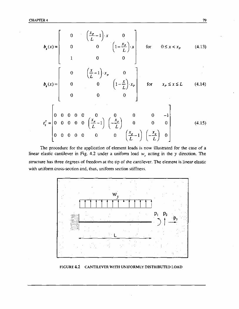
CHAPTER 4
0 (~-l}X 0
bg (X) = 0 0 (1- X{}x
1 0 0
0 (~ -1}Xp 0
bg (x) = 0 0 (1- ~}Xp 0 0 0
00000 0 0 o o t; = 0 0 0 0 0 (i -1) (- i)
o 0 0 0 0 o o
for
for
o o
o ~ x < xp
xp ~ x S L
-1
o
79
(4.13)
(4.14)
(4.15)
The procedure for the application of element loads is now illustrated for the case of a linear elastic cantilever in Fig. 4.2 under a uniform load Wy acting in the y direction. The
structure has three degrees of freedom at the tip of the cantilever. The element is linear elastic
with uniform cross-section and, thus, uniform section stiffness.
tff!l!f!f!f!l!
L ..
FIGURE 4.2 CANTILEVER WITH UNIFORMLY DISTRIBUTED LOAD
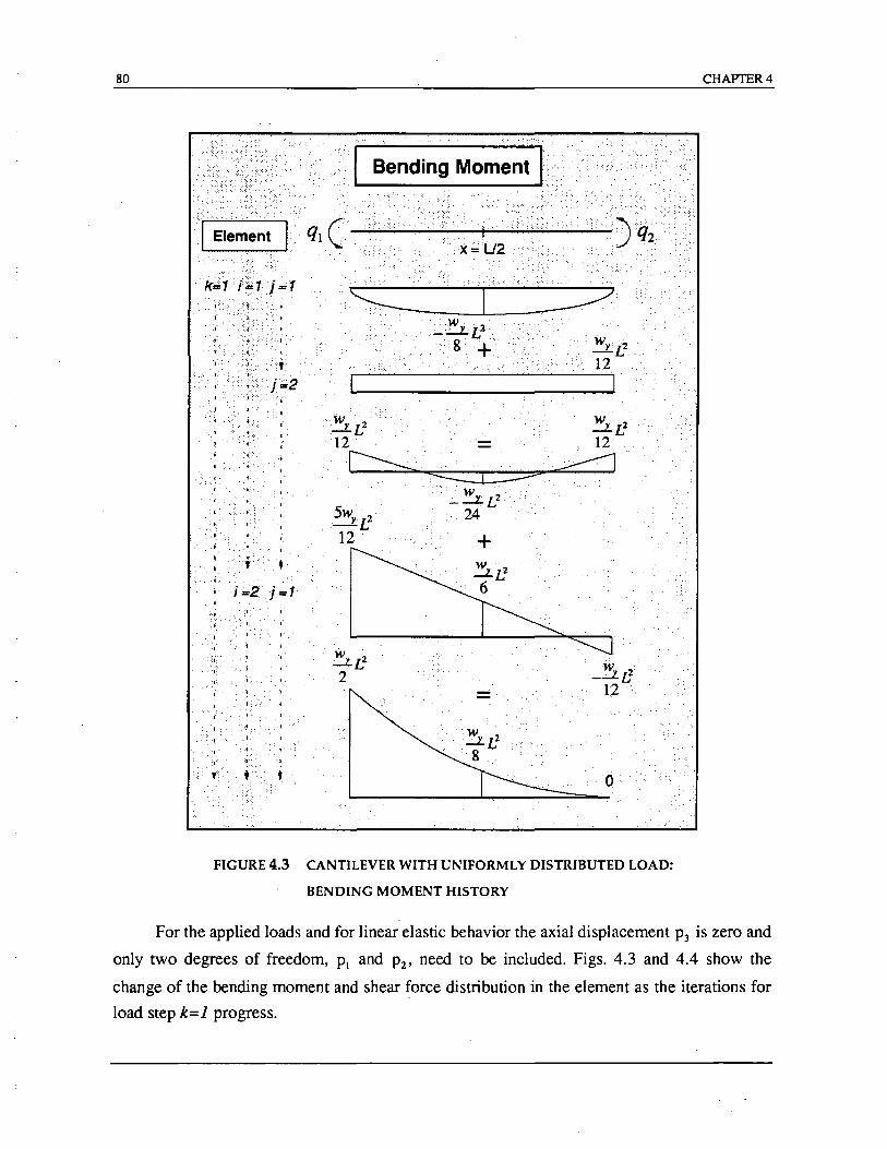
80
. ,
.,
.,
·f.
1';'2 ·:I~1
..1· ····x;;,;V2
::' " '::;::::: >.: : ~ : - : ' .. . . . _---L-I_.<::.: .. :.-.::.:.:~.:.·
Wy 2 -L 12 .~
0:::::::::::::: ·:····W ..
.:----Le 24
+
-.
_W_YL2
. 12
. "--z::::::1
W" 2 ":'..;..J..t 12
FIGURE 4.3 CANTILEVER WITH UNIFORMLY DISTRIBUTED LOAD:
BENDING MOMENT HISTORY
CHAPTER4
For the applied loads and for linear elastic behavior the axial displacement P3 is zero and
only two degrees of freedom, PI and P2' need to be included. Figs. 4.3 and 4.4 show the
change of the bending moment and shear force distribution in the element as the iterations for
load step k=l progress.
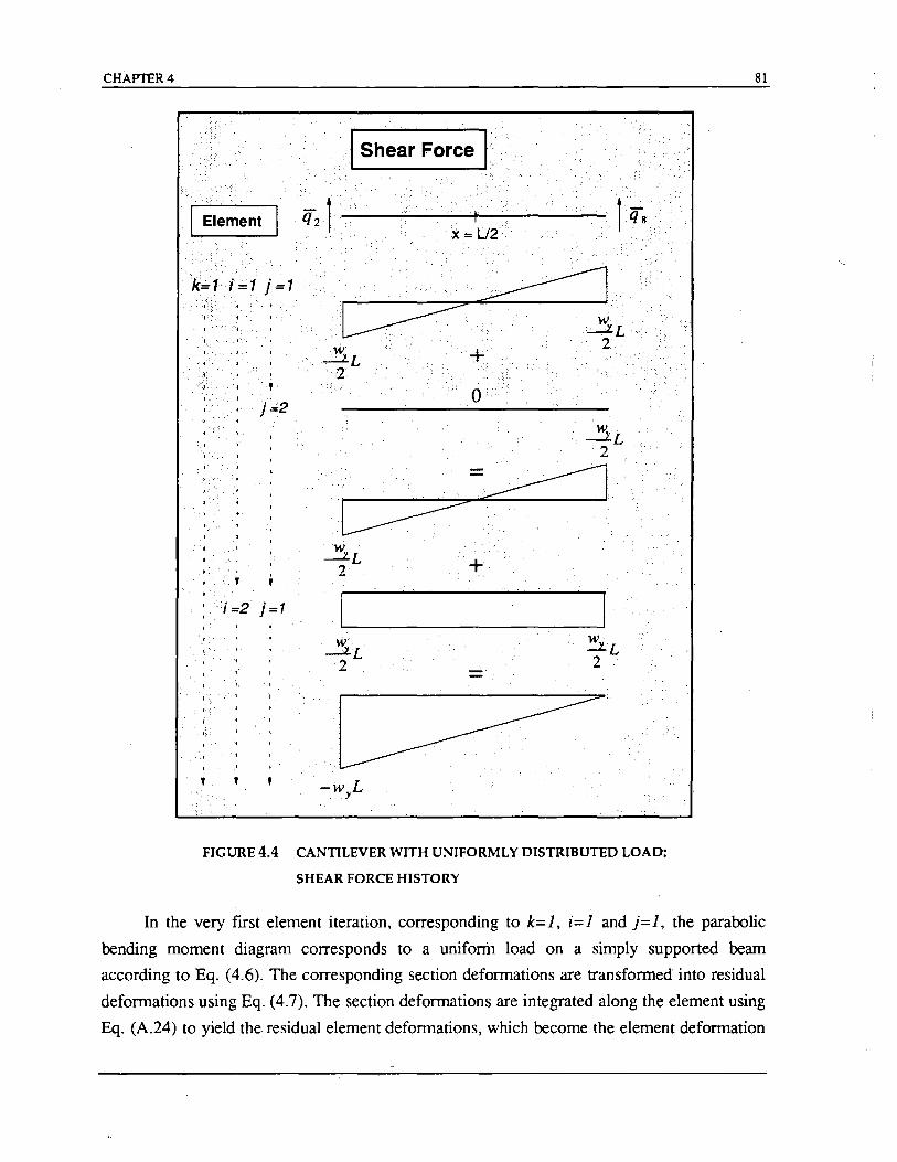
CHAPTER 4
."::/ : :.
'I::' .. "-1
.. ,
,.
, ..
.'
" I' ,
t",
,":.'
'1" '".
,
·1 Shear Force ,.
q 2 t.· · .• _i :-. ----,"----'---+-1--. ----x=U2
.3£ 2
...... =~
.~ ..... : .................• :
+
.3:.[ 2
~ .........................•... . .
-'w L 'j
FIGURE 4.4 CANTILEVER WITH UNIFORMLY DISTRIBUTED LOAD:
SHEAR FORCE HISTORY
81
In the very fIrst element iteration, corresponding to k=1, i=1 and j=1, the parabolic
bending moment diagram corresponds to a uniform load on a simply supported beam
according to Eq. (4.6). The corresponding section deformations are transformed into residual
deformations using Eq. (4.7). The section deformations are integrated along the element using
Eq. (A.24) to yield the residual element deformations, which become the element deformation

82 CHAP1ER4
increments for the following iteration, corresponding to k=l, i=l and j=2. The element
defonnations are transfonned into element force incremerits with Eq. (A.6). For a linear elastic element the element force increments are the well known fixed end moments wyL
2 /12.
At this point the element has converged and its bending moment diagram corresponds to that
of a beam that is fixed at both ends. In order to inclu~e the rigid body modes according to Eq. (4.8) two vertical forces wy Lj2 are added to the element resisting forces Q and
equilibrium is checked at the structure level. Since no external loads are applied to the structure, an unbalanced moment of wy L2 /12 and an unbalanced shear force of wy Lj2 now
act at the free end of the cantilever. These need to be applied as nodal forces with opposite
sign in the next Newton-Raphson iteration corresponding to k=l and i=2 in order to restore
equilibrium at the structure degrees of freedom. During the first element iteration of the new
Newton-Raphson iteration, i.e. for k= 1, i =2 and j= 1, a linear bending moment distribution is
added to the existing moments in the cantilever, as shown in Fig. 4.3. Since the can~lever is
linear elastic, element convergence is reached immediately. Because convergence is also
reached at the structural level, the analysis is complete. The final bending moment diagram is
the well known parabola shown at the bottom of Fig. 4.3. The evolution of all element and
structural vectors for this example is given in detail in Appendix B.
. The selected example is very simple, since the element is linear elastic and has a uniform
cross section. The proposed procedure for the application of element loads is, however,
general and can be applied for any material behavior and for any distribution of element loads.
In the general case of nonlinear material behavior and non-uniform cross section properties of
the element more iterations at the element and structure level are necessary for satisfying the
equilibrium and compatibility requirements under the applied element loads.
The same procedure is also used in the implementation of the beam-column element in
program FEAP, but the rigid body modes are included in a different way. In the stand alone
program, no forces due to element loads are applied at the structure degrees of freedom, so
that on convergence no forces act at the structural nodes. In other words the element loads
are treated as an initial force distribution. In program FEAP the shear forces that result from
the applied element loads when the rigid body modes are included according to Eq. (4.8) are
applied as forces at the structure degrees of freedom. The remainder of the process is identical
to that described previously, except that Eq. (4.8) is now bypassed. This alternative scheme is
more similar to the procedure that is typically followed in a stiffness-based element where
element loads are transformed into equivalent nodal loads.
In the implementation of this procedure in program FEAP for the linear elastic
CHAPTER 4 83
cantilever under uniform load the element has non zero end deformations (( MQI)')I during
the fIrst iteration (k=l, i=l and j=J) caused by a vertical force of (p~y =- wyL/2. The
parabolic bending moment diagram for a simply supported beam under a uniform load is then 1
added to the linear diagram that results from the non zero end deformations (( MQI f) . This
minor change facilitates the implementation of the element load ,Procedure in an existing finite
elemerit program.
4.6 Material S9ftening and Unloading in Reinforced Concrete Members
The nonlinear solution procedure that is proposed in the present study is particularly
suitable for modeling the softening behavior of reinforced concrete members. Even though the
algorithm is described here with reference to a fiber beam-column element, the procedure can
be used in structural members with any continuous nonlinear or piece-wise linear section
force-deformation relation. Spacone et al. (1992) discuss the implementation of the method in
the context of a differential moment-curvature relation. The method can also be extended to
the nonlinear analysis of other types of systems. The extension of the theory to systems made
up of several components in series and/or in parallel suitable for the nonlinear analysis of
prestressed concrete members with bonded or unbonded, internal or external tendons is the
subject of another current study.
In the discussion about softening it is important to underline the distinction between
softening of the entire structure and softening of certain members in a stiffening structure.
Softening of the entire structure is very difficult to simulate from a numerical standpoint and
the general Newton-Raphson method is not suitable for the task. Special iterative strategies,
such as the arc-length method, or ad-hoc procedures, such as displacement control analysIs,
should be used in this case, but such discussion is beyond the scope of the present study.
The state determination process of the nonlinear analysis of a structure involves the
application of end displacements on the structural elements. Consequently, tracing the
softening response of elements under displacement control conditions is computationally
easier than tracing the softening response of the structure. Even so, element softening is a very
challenging numerical problem and there is growing interest in the development of a reliable
solution method, especially for the response analysis of reinforced concrete structures under
strong ground motions. Element softening plays an important role in the assessment of global
and local ductility demands of structures under intense ground shaking when some members
might reach their capacity and start experiencing strength softening. While force redistribution
84 CHAPTER 4
might lead to an increase of the lateral load capacity of the structure, the defonnation ductility
demand of softening members might be so high, that partial or total collapse will take place
before the structure reaches its lateral load capacity.
From a theoretical standpoint the flexibility method is ideally suited for modeling the
softening behavior of reinforced concrete elements. When an element exhibits strain softening
at the end sections, the moments decrease along the element and non-softening sections
unload to satisfy equilibrium. Since in the absence of element loads the moment distribution
along the element is always linear, this behavior is captured by the flexibility method. Such
softening and unloading behavior is much harder to represent with a classical stiffness-based
two-node element in which the curvature distribution is assumed linear. In such case several
elements are needed to approximate the actual nonlinear curvature distribution and numerical
difficulties can, nonetheless, arise as discussed in Section 1.2.3 and Fig. 1.9, which is
excerpted from Zeris and Mahin (1988). A comparison of the two types of element
fonnulation is presented in Spacone et al. (1992).
The application of the proposed solution algorithm to the case of a softening element is
first discussed from a theoretical standpoint and, subsequently, illustrated with a simple
. example. For the sake of simplicity superscript k that denotes the current load step js omitted
in the following discussion. The discussion starts when the structure is at the beginning of
Newton-Raphson iteration i and with the assumption that. the stiffness matrices K i-
I of all
elements at the end of the last iteration are positive definite. At the stan of the new iteration
the defonnation increments tlqi are imposed on the elements and the resulting. element force
increments (MQi)j . are convened to section force increments (Mli(x)Y through force
interpolation functi?ns. The section force increrrie~ts (Mf)i (x) Y cause section defonnation
increments according to Eq. (A .12) which are added to the previous section defonnations to
yield the new total defonnations (di (x) y. Consider the case that upon completion of the
section state detennination for the new total defonnations (di(x)Y one section exhibits
softening, so that its stiffness changes from posi tive definite (ki (x) y-l to negative definite
(ki(X)y. The unbalanced forces (MJ~(x»)j are positive, while the residual section
defonnations
are negative. The element stiffness is updated with Eqs. (A.22) and (A.23). Assuming that the
entire element stiffnes~ has also changed from positive definite (Ki)j-l to negative definite
(KT and that Eq. (A.24) also returns negative residual defonnations (SiY at the element
CHAPTER 4 85
ends, it is concluded from Eq. (A.6) that the new force increments (MQi)j+l are also negative.
The element has, thus, detected the fact that, under the new deformations qi, it can resist a
smaller force than that predicted with the stiffness of the previous converged state. The
negative unbalanced forces at the element ends are convened to negative se,ction force
increments (Mli (x) )j+l based on the force interpolation functions and the corresponding
section deformation increments (Mdi(X))j+l are obtained with Eq. (A.12). At the section that
exhibited softening in the previous iteration j the sign of the deformation increments depends on the size of the positive increments (/(x))j . (DMi(x))j+l relative to the negative residual
deformations (ri (x) y. In either case it is important to note that the section resisting force is
reduced.
Once the element converges, it is very likely that the current element stiffness matrix is
negative definite. The structure stiffness matrix is assembled from all element stiffness
matrices and another load increment is applied to the structure. Since the structure stiffness
matrix is still positive definite, the structure is capable of resisting a higher load, even though
one element is softening. The new deformation increments llqi+l at the element ends give rise
to negative force increments in the softening element as a result of the multiplication of the
negative stiffness matrix Ki with positive deformation increments llqi+l. Thus, the softening
element continues to unload, while the hardening members now resist a greater ponion of the
applied load increment. At the same time the softening element contributes a larger ponion of
the deformation of the structure.
This brief description underlines the fact that no special steps need to be taken for the
treatment of softening elements in the proposed analysis method. Within the algorithm the
transition from a positive to a negative element stiffness matrix does not have to be detected
and, both, positive and negative deformation increments, deformation corrections, force
increments, unbalanced forces, and, finally, stiffness and flexibility matrices at the section as
well as at the element level can be accommodated. Consequently, unloading of elements is
also treated without requiring a reduction of load step size or special computational steps.
The advantage of the proposed method in the analysis of softening systems can be best
illustrated with a simple example that is shown in Fig. 4.5. It consists of two extensional
springs connected in series. Spring A is linear elastic, while spring B is bilinear elastic so-ain
softening. In a series model the system deformation is the sum of the component
deformations, while the element forces are equal to the force applied on the entire system. For
the two spring system and with the notation of Fig. 4.5 these conditions can be written as:
Q=DA =DB
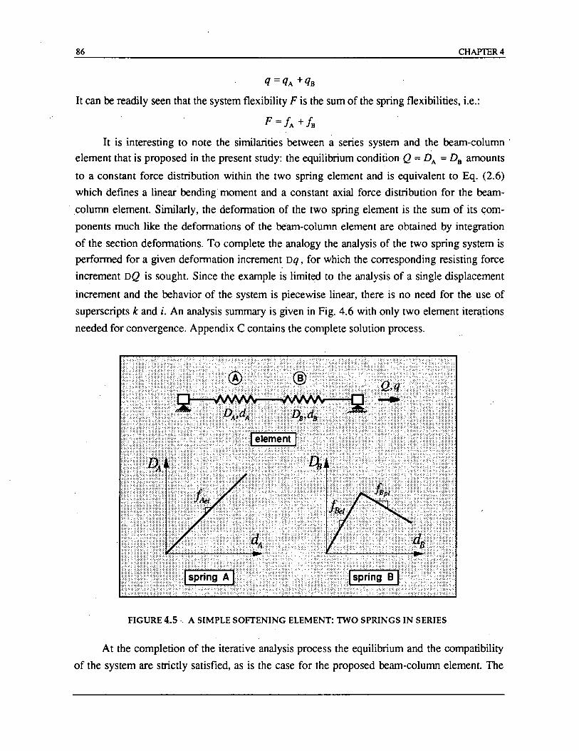
86 CHAP1ER4
q = qA +qB
It can be readily seen that the system flexibility F is the sum of the spring flexibilities, i.e.:
F = fA + fB It is interesting to note the similarities between a series system and the beam-column
element that is proposed in the present study: the equilibrium condition Q = DA = DB amounts
to a constant force distribution within the two spring element and is equivalent to Eq. (2.6)
which defines a linear bending moment and a constant axial force distribution for the beam-
, ,column element. Similarly, the deformation of the two spring element is the sum of its com
ponents much like the deformations of the beam-column element are obtained by integration
of the section deformations. To complete the analogy the analysis of the two spring system is
performed for a given deformation increment Dq, for which the corresponding resisting force
increment DQ is sought. Since the example is limited (0 the analysis of a single displacement
increment and the behavior of the system is piecewise linear, there is no need for the use of
superscripts k and i. An analysis summary is given in Fig. 4.6 with only two element iteI"a:tions
needed for convergence. Appendix C contains the complete solution process.
FIGURE 4.5 " A SIMPLE SOFTENING ELEMENT: TWO SPRINGS IN SERIES
At the completion of the iterative analysis process the equilibrium and the compatibility
of the system are strictly satisfied, as is the case for the proposed beam-column element. The
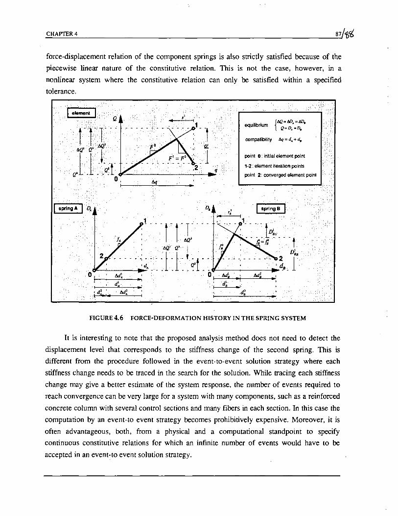
_C_H_A~ ___ R_4 ______________________________________________________ ~87/~i
force-displacement relation of the component springs is also strictly satisfied because of the
piecewise linear nature of the constitutive relation. This is not the case, however, in a
nonlinear system where the constitutive relation can only be satisfied within a specified
tolerance.
I-element
: 1
- , , ! -1. 'T' " -, -- - _ . dQ'
{t.Q = IlD = 1lD.
equilibrium Q=D:=D.
compatibility llq = d. + <4
point 0: initiat element point
',2: etement iteration points
point 2: converged element point
1 ._
'. '.'- ',P~. ".' • ~=f, _ I
2 --: _11
1'1' Q
1' I - .
,'- - - -, -:~A~·._~ ~.- -~~: ~1 ~ ~~~ o I-I-=:L-+r---'-=-+
.) . I
,d~ , __ -I.. d.,.
fyJ' A
M,
d~ -, I
-I lid' , B • ,
.. I
d; •
FIGURE 4.6 FORCE-DEFORMATION HISTORY IN THE SPRING SYSTEM
It is interesting to note that the proposed analysis method does not need to detect the
displacement level that corresponds to the stiffness change of the second spring. This is
different from the procedure followed in the event-to-event solution strategy where each
stiffness change needs to be traced in the search for the solution. While tracing each stiffness
change may give a better estimate of the system response, the number of events required to
reach convergence can be very large for a system with many components, such as a reinforced
concrete column with several control sections and many fibers in each section, In this case the
computation by an event-to event strategy becomes prohibitively expensive. Moreover, it is
often advantageous, both, from a physical and a computational standpoint to specify
continuous constitutive relations for which an infinite number of events would have to be
accepted in an event-to event solution strategy.

5.1 General
CHAPTERS
APPLICATIONS
A series of examples are presented in this chapter to demonstrate the ability of the
proposed element to describe the hysteretic behavior of reinforced concrete beams and
columns under imposed cyclic load and defonnation histories. The analytical results in this
chapter are obtained with the stand alone program BEAMCOL whose numerical
implementation was discussed in the previous chapter.
When experiments are conducted, loads are applied to the specimen in a controlled
fashion and the resulting displacements and deformations are measured. Typically, members
that exhibit a relatively high stiffness are tested by controlling the force applied on the
specimen. Once significant damage and stiffness deterioration of the specimen sets in, the test
is continued under displacement control, whereby the applied forces are carefully adjusted in
order to produce a given displacement history. In the numerical simulation of experiments a
single method of load application has to the used for the entire analysis, since most finite
element programs do not permit changes in the boundary conditions during the analysis.
Numerical simulations under force control provide good results when the member stiffness is
high, but fail to trace the nonlinear behavior near the ultimate strength of the member and the
post-peak: response. For this reason the numerical simulations in this chapter were conducted
under displacement control.
Three tests have been selected for the verification of the proposed beam-column
element. The tests comprise two reinforced concrete cantilever beams and a reinforced
concrete beam-column. The first beam is selected for the study of the moment-curvature
behavior of a single section and for the study of the effect of different tolerance measures and
displacement increments on the accuracy of the analytical results. The second specimen is a
cantilever beam under uniaxial bending and the third specimen is a cantilever column that was
subjected to a constant axial force in combination with uniaxial and biaxial bending, both,
monotonic and cyclic. For each test the geometry and the material characteristics of the
specimen as well as the parameters of the material models for concrete and reinforcing steel
are given. The material parameters are obtained from available experimental information from
89

90 CHAPTERS
coupon or concrete cylinder tests. Finally, the load and displacement history of the specimen
and the boundary conditions used in the analysis are also specified.
The chapter concludes with a parameter study of the third specimen, the cantilever
column. This study aims at investigating the sensitivity of the proposed model to the number
of control sections within the column, both, in the presence and in the absence of an axial
compressive force. It is important in this regard to establish whether the analytical results
converge to the actual solution as the number of control sections in the column increases and,
if so, to determine the smallest number of column control sections that yield sufficiently
accurate results.
5.2 Moment-Curvature of a Section
Kaba and Mahin (1983) proposed a nonlinear method for describing the hysteretic
behavior of reinforced concrete sections as was briefly discussed in the literature survey of
Chapter 1. Their model is compared with the experimental response of a concrete cantilever
beam tested by Kent (1969). The same experimental results are used here to test the validity
of the beam-column element proposed in this study. The geometry of the specimen and the
geometry of the cross section as well as the discretization used by Kaba and Mahin, are shown
in Fig. 5.1 and summarized in Table 5.1. The material parameters for the concrete and
reinforcing steel models are summarized in Tables 5.2 and 5.3, respectively.
r .~ ........ I_· ___.----.,--'1 •
]00*
1 element
4SeC~omi .
Material Type and Number of Fibers
o Unconfined Concrete: 4 • 2 • 2 + 10 .2
I>::}:::l Confined Conerele: 12 .2
_ sreel:4
z
FIGURE 5.1 STRUCTURE DISCRETIZATION FOR KENT BEAM # 24
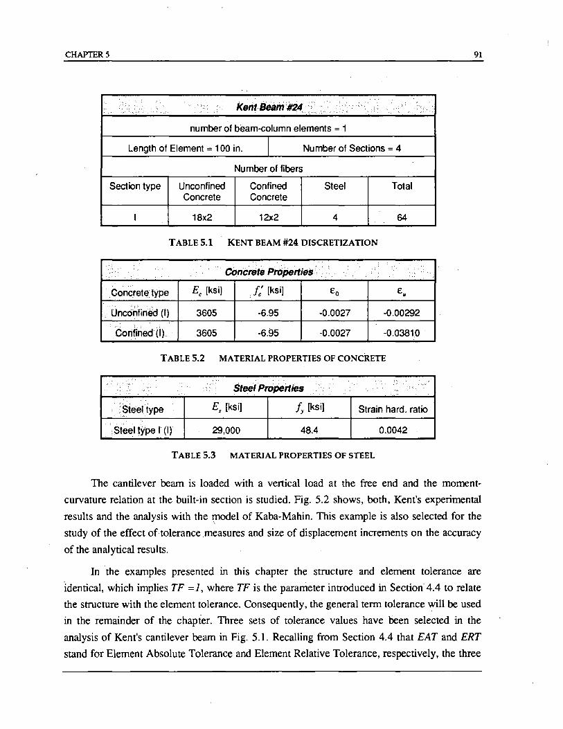
CHAPTERS 91
kent Beanf#24 .. . ..• .......
...... "-.-:~ .. . . ' .... ~ ••. <...... ... ........... ..Q
number of beam-column elements = 1
Length of Element = 100 in. I Nu mber of Sections = 4
Number of fibers
Section type Unconfined Confined Steel Total Concrete Concrete
I 18x2 12x2 4 64
TABLE 5.1 KENT BEAM #24 DISCRETIZATION
: ............. COncrete proPerties ..': .....
Concrete type Ec [ksiJ f: [ksiJ Eo E"
.•... Unconfined (I) 3605 -6.95 -0.0027 -0.00292 .
Confined (I) 3605 -6.95 -0.0027 -0.03810
TABLE 5.2 MATERIAL PROPERTIES OF CONCRETE
•••••••••••• Steel Properties
.
I .
>Steeltype Es [ksiJ Iy [ksiJ Strain hard. ratio
Steel tyPe r (I) 29,000 48.4 0.0042
TABLE 5.3 MATERIAL PROPERTIES OF STEEL
The cantilever beam is loaded with a vertical load at the free end and the moment
curvature relation at the built-in section is studied. Fig. 5.2 shows, both, Kent's experimental
results and the analysis with the ~odel of Kaba-Mahin. This example is also selected for the
study of the effect of tolerance measures and size of displacement increments on the accuracy
of the analytical results.
In the examples presented in this chapter the structure and element tolerance are
identical, which implies TF = 1, where TF is the parameter introduced in Section 4.4 to relate
the structure with the element tolerance. Consequently, the general term tolerance will be used
in the remainder of the chapter. Three sets of tolerance values have been selected in the
analysis of Kent's cantilever beam in Fig. 5.1. Recalling from Section 4.4 that EAT and ERT
stand for Element Absolute Tolerance and Element Relative Tolerance, respectively, the three
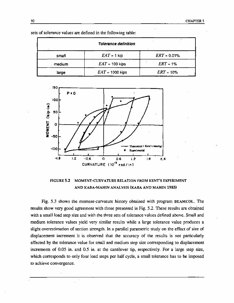
92 CHAPTERS
sets of tolerance values are defined in the following table:
Tolerance definition
small EAT = 1 kip ERT = 0.01%
medium EAT = 100 kips ERT= 1%
large EAT = 1000 kips ERT= 10%
r50r---------------,-------------------__ ~
100
·roo
-1.8
P=o.
- ThtocelicaJ « Kent's resul~
• ExperimlllW
1.2 -0.6 0 0.6 1.2 1.8 2.4
CURVATUR E (IO-l r ad lin)
,
FIGURE S.2 MOMENT-CURVATURE RELA nON FROM KENT'S EXPERIMENT
AND KABA-MAHIN ANALYSIS (KABA AND MAHIN 1983)
Fig. 5.3 shows the moment-curvature history obtained with program BEAMCOL. The
results show very good agreement with those presented in Fig. 5.2. These results are obtained
with a small load step size and with the three sets of tolerance values defined above. Small and
medium tolerance values yield very similar results while a large tolerance value produces a
slight overestimation of section strength. In a parallel parametric study on the effect of size of
displacement increment it· is observed that the accuracy of the results is not particularly
affected by the tolerance value for small and medium step size corresponding to displacement
increments of 0.05 in. and 0.5 in. at the cantilever tip, respectively. For a large step size,
which corresponds to only four load steps per half cycle, a small tolerance has to be imposed
to achieve convergence.
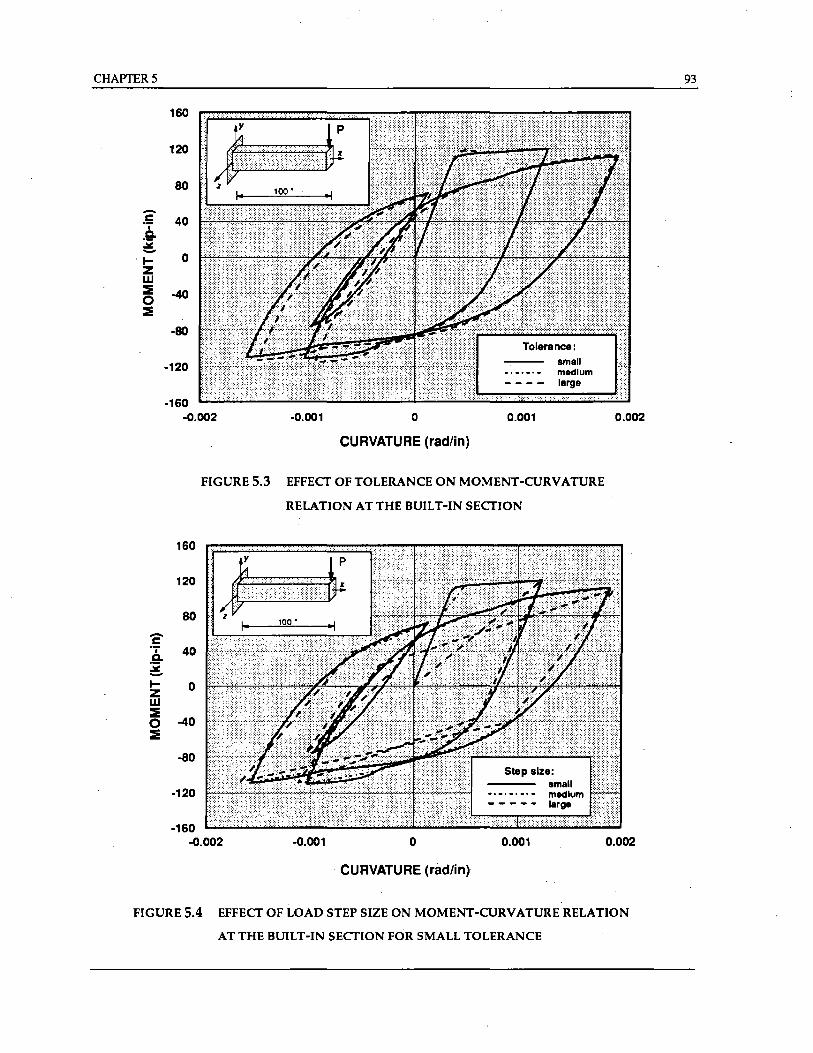
CHAPTERS
-c " .9-.:.:: -01-Z UJ :iE o :iE
160
120
80
40
o
-40
-80
-120
-160 -0.002 -0.001 o
CURVATURE (rad/in)
0.001
small medium large
FIGURE 5.3 EFFECf OF TOLERANCE ON MOMENT-CURVATURE
RELATION AT THE BUILT-IN SECfION
160
'J~ .. o.oo.<
80 z
120
-c " 40 Q,
:i -I- 0 z UJ :iE o -40 :iE
-80
-120
-160 -0.002 -0.001 o
CURVATURE (rad/in)
Slap size: small medium
- - - - - large
0.001
0.002
0.002
FIGURE 5.4 EFFECf OF LOAD STEP SIZE ON MOMENT-CURVATURE RELATION
AT THE BUILT-IN SECfION FOR SMALL TOLERANCE
93
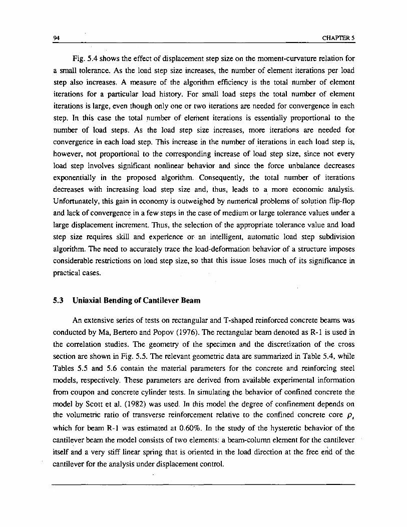
94 CHAPTERS
Fig. 5.4 shows the effect of displacement step size on the moment-curvature relation for
a small tolerance. As the load step size increases, the number of element iterations per load
step also increases. A measure of the algorithm efficiency is the total number of element
iterations for a particular load history. For small load steps the total number of element
iterations is large, even though only one or two iterations are needed for convergence in each
step. In this case the total number of element iterations is essentially proportional to the
number of load steps. As the load step size increases, more iterations are needed for
convergerice in each load step. This increase in the number of iterations in each load step is,
however, not proportional to the corresponding increase of load step size, since not every
load step involves significant nonlinear behavior and since the force unbalance decreases
exponentially in the proposed algorithm. Consequently, the total number of iterations
decreases with increasing load step size and, thus, leads to a more economic analysis.
Unfortunately, this gain in economy is outweighed by numerical problems of solution flip-flop
and lack of convergence in a few steps in the case of medium or large tolerance values under a
large displacement increment. Thus, the selection of the appropriate tolerance value and load
step size requires skill and experience or- an intelligent, automatic load step subdivision
algorithm. The need to accurately trace the load-deformation behavior of a structure imposes
considerable restrictions on load step size, so that this issue loses much of its significance in
practical cases.
5.3 Uniaxial Bending of Cantilever Beam
An extensive series of tests on rectangular and T -shaped reinforced concrete beams was
conducted by Ma, Bertero and Popov (1976). The rectangular beam denoted as R-l is used in
the correlation studies. The geometry of the specimen and the discretization of the cross
section are shown in Fig. 5.5. The relevant geometric data are summarized in Table 5.4, while
Tables 5.5 and 5.6 contain the material parameters for the concrete and reinforcing steel
models, respectively.· These parameters are derived from available experimental information
from coupon and concrete cylinder tests. In simulating the behavior of confined concrete the
model by Scott et al. (1982) was used. In this model the degree of confinement depends on the volumetric ratio of transverse reinforcement relative to the confined concrete core Ps
which for beam R-I was estimated at 0.60%. In the study of the hysteretic behavior of the
cantilever beam the model consists of two elements: a beam-column element for the cantilever
itself and a very stiff linear spring that is oriented in the load direction at the free end of the
cantilever for the analysis under displacement control.
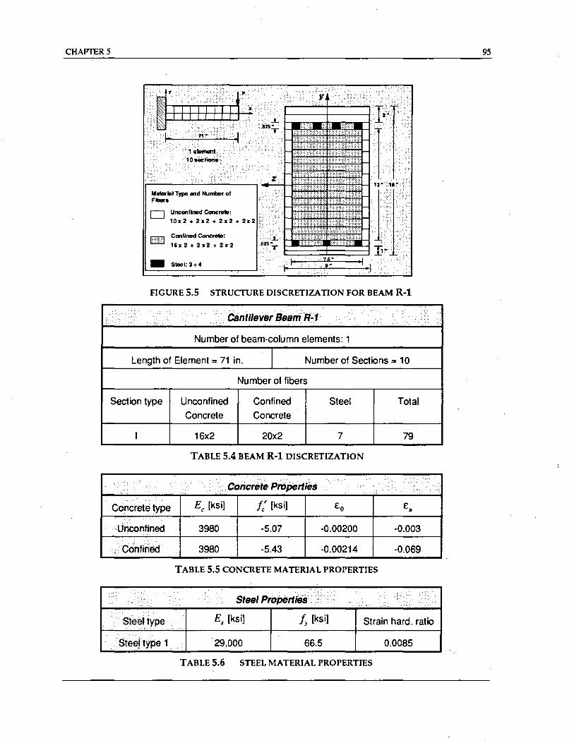
CHAPTER 5
o Unconnned Concrete:
10.2 + 2.2 + 2.2 + 2.2
Confined Concrete:
16.2+2.2+2.2
_ Sleel: 3+4
FIGURE 5.5 STRUcruRE DISCRETIZATION FOR BEAM R-l
•••••••••••••••••••••••• ....•. ·..CantileverBesmR~1
• ••• ..... / ......
Number of beam-column elements: 1
Length of Element = 71 in. I Number of Sections = 10
Number of fibers
Section type Unconfined Confined Steel Total
Concrete Concrete
I 16x2 20x2 7 79
TABLE 5.4 BEAM R-l DISCRETIZATION
. ... •.• . ConcrfJte Properties •• .................•..
... . ... . ...
C()ncrete type Ec [ksi] t: [ksi] Eo E" .
.. Uriconfiried 3980 -5.07 -0.00200 -0.003
6····(00· ···onm 3980 -5.43 -0.00214 -0.069
TABLE 5.5 CONCRETE MATERIAL PROPERTIES
. Steel PropertieS
Es [ksi] /y [ksi] Strain hard. ratio
Steel type 1 . . • ·29,000 66.5 0.0085
TABLE 5.6 STEEL MATERIAL PROPERTIES
95
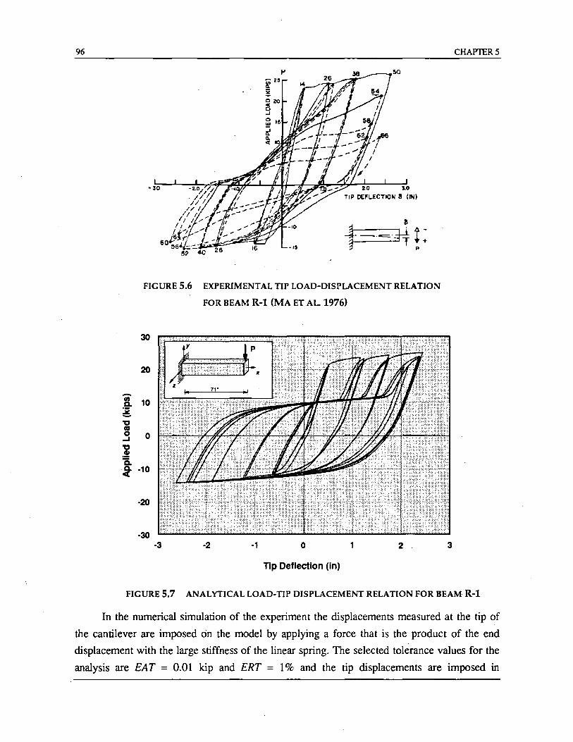
96
FIGURE 5.6 EXPERIMENTAL TIP LOAD-DISPLACEMENT RELATION
FOR BEAM R-1 (MA ET AL. 1976)
30
20
-! 10 ~ -" o ~ ..J
~ C. -~ -10
-20
-30 -3 -2 -1 o 2
TIp Deflection (in)
CHAPTERS
3
FIGURE 5.7 ANALYTICAL LOAD-TIP DISPLACEMENT RELATION FOR BEAM R-1
In the numerical simulation of the experiment the displacements measured at the tip of
the cantilever are imposed on the model by applying a force that is the product of the end
displacement with the large stiffness of the linear spring. The selected tolerance values for the
analysis are EAT = 0.01 kip and ERT = 1 % and the tip displacements are imposed in
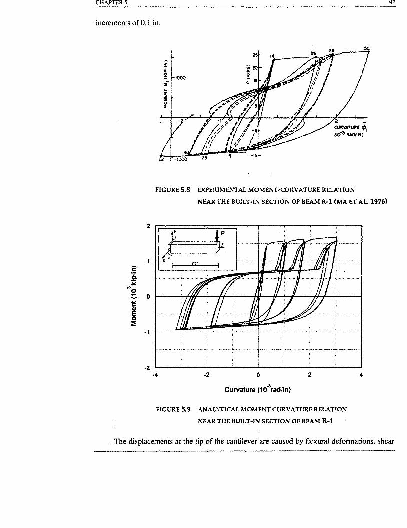
CHAPTERS
increments of 0.1 in.
2
1 -c :~ .:.::
t'> Q ... 0 -'E Q)
e 0 :E
-1
-2
FIGURE 5.8 EXPERIMENTAL MOMENT~CURVATURE RELATION
NEAR THE BUILT-IN SECTION OF BEAM R-l (MA ET AL. 1976)
1; ~ :::
z I· 71· -I
',- ,- ·····r·············
-,' "~' ~ ............. ~ .. : .... -...... ~ ....... --.... -+ ... ~ .. ~ ......... -.... - .. ~-. -_ ......... -............. .
-4 -2 o
Curvature (10·3rad/in)
2
FIGURE 5.9 ANALYTICAL MOMENT CURVATURE RELATION
NEAR THE BUlL T ~IN SECTION OF BEAM R-1
4
97
. The displacements at the rip of the cantilever are caused by flexural defonnations, shear
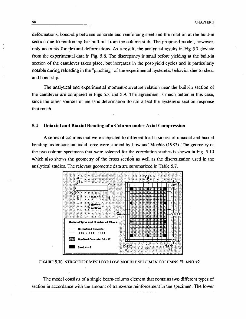
98 CHAP1ER5
defonnations, bond-slip between concrete and reinforcing steel and the rotation at the built-in
section due to reinforcing bar pull-out from the column stub. The proposed model, however,
"only accounts for flexural defonnations. As a result, the analytical results in Fig 5.7 deviate
from the experimental data in Fig. 5.6. The discrepancy is small before yielding at the built-in
section of the cantilever takes place, but increases in the post-yield cycles and is particularly·
notable during reloading in the "pinching" of the experimental hysteretic behavior due to shear
and bond-slip.
The analytical and experimental moment-curvature relation near the built-in section of
the cantilever are compared in Figs 5.8 and 5.9. The agreement is much better in this case,
since the other sources of inelastic defonnation do not affect the hysteretic section response
that much.
5.4 Uniaxial and Biaxial Bending of a Column under Axial Compression
A series of columns that were subjected to different load histories of uniaxial and biaxial
bending under constant axial force were studied by Low and Moehle (1987). The geometry of
the two column specimens that were selected for the correlation studies is shown in Fig. 5.10
which also shows the geometry of the cross section as well as the discretization used in the
analytical studies. The relevant geometric data are summarized in Table 5.7.
D
-Unconllned Concrete: 4.8+4.4+11.4
Conlroed Concrete: 16. 12
Steel: 4 + 6
FIGURE 5.10 STRUClURE MESH FOR LOW-MOEHLE SPECIMEN COLUMNS #1 AND #2
The model consists of a single beam-column element that contains two different types of
section in accordance with the amount of transverse reinforcement in the specimen. The lower
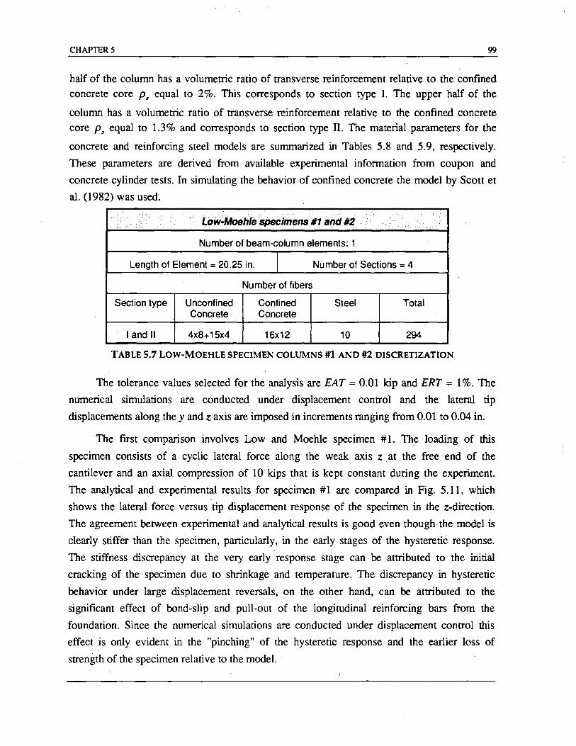
CHAPTERS 99
half of the column has a volumetric ratio of transverse reinforcement relative to the confined concrete core p. equal to 2%. This corresponds to section type I. The upper half of the
column has a volumetric ratio of transverse reinforcement relative to the confined concrete
core p. equal to 1.3% and corresponds to section type II. The material parameters for the
concrete and reinforcing steel models are summarized in Tables 5.8 and 5.9, respectively.
These parameters are derived from available experimental information from coupon and
concrete cylinder tests. In simulating the behavior of confined concrete the model by Scott et
aI. (1982) was used .
.. ,<. l.o"'~MoehleSpecimens #1 and #2 ..
. .
. " . ." - -, - .
Number of beam-column elements: 1
Length of Element = 20.25 in. I Number of Sections = 4
Number of fibers
Section type Unconfined Confined Steel Total Concrete Concrete
I and II 4x8+15x4 16x12 10 294
TABLE 5.7 Low-MOEHLE SPECIMEN COLUMNS #1 AND #2 DISCRETIZATION
The tolerance values selected for the analysis are EAT = 0.01 kip and ERT = 1 %. The
numerical simulations are conducted under displacement control and the lateral tip
displacements along the y and z axis are imposed in increments ranging from 0.01 to 0.04 in.
The first comparison involves Low and Moehle specimen #1. The loading of this
specimen consists of a cyclic lateral force along the weak axis z . at the free end of the
cantilever and an axial compression of 10 kips that is kept constant during the experiment.
The analytical and experimental results for specimen #1 are compared in Fig. 5.11, which
shows the lateral force versus tip displacement response of the specimen in the z-direction.
The agreement between experimental and analytical results is good even though the model is
clearly stiffer than the specimen, particularly, in the early stages of the hysteretic response.
The stiffness discrepancy at the very early response stage can be attributed to the initial
cracking of the specimen due to shrinkage and temperature. The discrepancy in hysteretic
behavior under large displacement reversals, on the other hand, can be attributed to the
significant effect of bond-slip and pull-out of the longitudinal reinforcing bars from the
foundation. Since the numerical simulations are conducted under displacement control this
effect is only evident in. the "pinching" of the hysteretic response and the earlier loss of
strength of the specimen relative to the rhodel. .
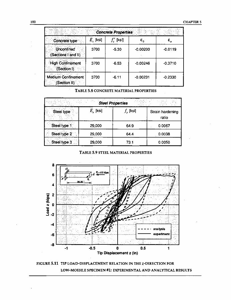
100
Ec [ksi] Ie' [kSi] EO
3700 -5.30 -0.00200 -0.0119
3700 -6.53 -0.00246 -0.3710
3700 -6.11 -0.00231 -0.2330
TABLE 5.8 CONCRETE MATERIAL PROPERTIES
'.- .. ' -'-." ..
Steel' type' .. . .. .
.' "' ...... . .... . ..... .... ' ..
. . Steertypet
steel type 2 , ... ' . .... ,. Steel tYpe 3
8
6
4
(;i'2 Co :i -N 0 'a as 0
...J ·2
-4
·6
·8 ·1
, .. '
·Steel Properties
Es [ksi] Iy [ksi]
29,000 64.9
29,000 64.4
29,000 73.1
.. '. . ,',
Strain hardening
ratio
0.0067
0.0038
0.0050
TABLE 5.9 STEEL MATERIAL PROPERTIES
-0.5 o 0.5 1 Tip Displacement z (in)
CHAPTERS
FIGURE 5.11 TIP LOAD-DISPLACEMENT RELATION IN THEz-DlRECTION FOR
LOW-MOEHLE SPECIMEN #1: EXPERIMENTAL AND ANALYTICAL RESULTS
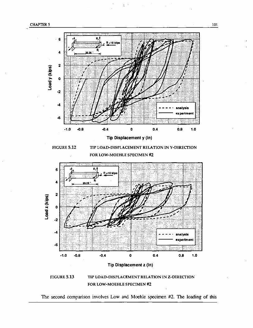
CHAPTERS
en .Q. ~ ->-"t:I ca .9
-.~ ~ N '0
8 ...J
6
4
2
0
-2
-4
-6
-1.0 -0.8
FIGURE 5.12
-0.4 o 0.4 0.8 1.0
Tip Displacement y (in)
TIP LOAD-DISPLACEMENT RELATION IN Y-DIRECTION
FOR LOW-MOEHLE SPECIMEN #2
6 •.•.••...•.•.••••• ~~Ips·
;';"";';'';'";''''''=-'-'-'-'''''Il.=''' 4
2
0
-2
-4
-6
-1.0 -0.8 -0.4 o 0~4 0.8 1.0
Tip Displacement z (in)
FIGURE 5.13 TIP LOAD-DISPLACEMENT R ELATION IN Z-DIRECTION
FOR LOW-MOEHLE SPECIMEN #2
101
The second comparison involves Low and Moehle specimen #2. The loading of this
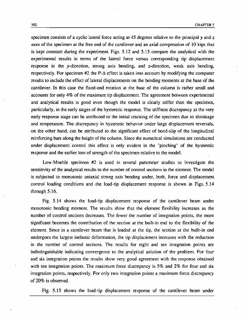
102 CHAPTERS
specimen consists of a cyclic lateral force acting at 45 degrees relative to the principal y and z axes of the specimen at the free end of the cantilever and an axial compression of 10 kips that
is kept constant during the experiment. Figs. 5.12 and 5.13 compare the analytical with the
experimental results in terms of the hueral force versus corresponding tip displacement
response in the y-direction, strong axis bending, and z-direction, weak axis bending,
respectively. For specimen #2 the p-~ effect is taken into account by modifying the computer
results to include the effect of lateral displacements on the bending moments at the base of the
cantilever. In this case the fixed-end rotation at the base of the column is rather small and
accounts for only 4% of the maximum tip displacement. The agreement between experimental
and analytical results is good even though the model is clearly stiffer than the specimen,
particularly. in the early stages of the hysteretic response. The stiffness discrepancy at the very
early response stage can be attributed to the initial cracking of the specimen due to shrinkage
and temperature. The discrepancy in hysteretic behavior under large displacement reversals,
on the other hand, can be attributed to the significant effect of bond-slip of the longitudinal
reinforcing bars along the height of the column. Since the numerical simulations are conducted
under displacement control this effect is only evident in the "pinching" of the hysteretic
response and the earlier loss of strength of the specimen relative to the model.
Low-Moehle specimen #2 is used in several parameter studies to investigate the
sensitivity of the analytical results to the number of control sections in the element. The model
is subjected to monotonic uniaxial strong axis bending under, both, force and displacement
control loading conditions and the load-tip displacement response is shown in Figs. 5.14
through 5.16.
Fig. 5.14 shows the load-tip disphtcement response of the cantilever beam under
monotonic bending moment. The results show that the element flexibility increases as the
number of control sections decreases. The fewer the number of integration points, the more
significant becomes the contribution of the section at the built-in end to the flexibility of the
element. Since in a cantilever beam that is loaded at the tip, the section at the built-in end
undergoes the largest inelastic deformation, the tip displacement increases with the reduction
in the number of control sections. The results for eight and ten integration points are
indistinguishable indicating convergence to the analytical solution of the problem. For four
and six integration points the results show very good agreement with the response obtained
with ten integration points. The maximum force discrepancy is 5% and 2% for four and six
integration points, respectively. For only two integration points a maximum force discrepancy
of 20% is observed .
. Fig. 5.15 shows the load-tip displacement response of the cantilever beam under
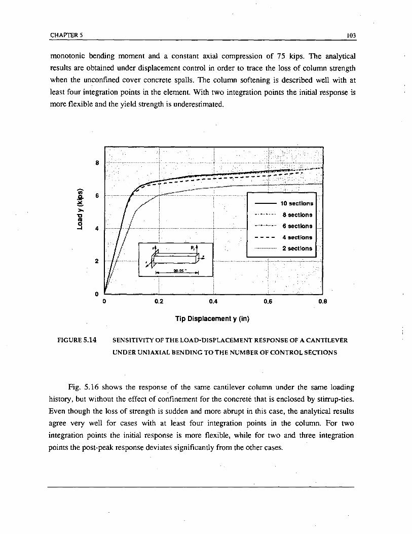
CHAPTERS 103
monotonic bending moment and a constant axial compression of 75 kips. The analytical
results are obtained under displacement control in order to trace the loss of column strength
when the unconfined cover concrete spalls. The column softening is described well with at
least four integration points in the element. With two integration points the initial response is
more flexible and the yield strength is underestimated.
8
o o
FIGURE 5.14
4 sections
:. ~~ I·················.··········m:::-:_~:':n •.... 0.2 0.4 0.6 0.8
Tip Displacement y (in)
SENSITIVITY OF THE LOAD-DISPLACEMENT RESPONSE OF A CANTILEVER
UNDER UNIAXIAL BENDING TO THE NUMBER OF CONTROL SECTIONS
Fig. 5.16 shows the response of the same cantilever column under the same loading
history, but without the effect of confinement for the concrete that is enclosed by stirrup-ties.
Even though the loss of strength is sudden and more abrupt in this case, the analytical results
agree very well for cases with at least four integration points in the column. For two
integration points the initial response is more flexible, while for two and three integration
points the post-peak response deviates significantly from the other cases.
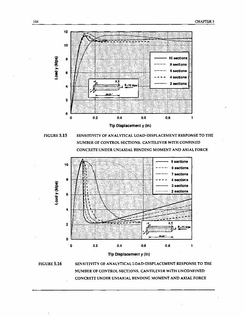
104
12
10
-II) 8 Co :;: ->-" 6 8 ~
4
2
0
FIGURES.IS
10
8 -(II a. :;: ->- 6
" co 0 ~
4
2
0 0.2 0.4 0.6
Tip Displacement y (in)
6 sections
4 sections
0.8
CHAPTER 5
1
SENSITIVITY OF ANAL YrICAL LOAD-DISPLACEMENT RESPONSE TO THE
NUMBER OF CONTROL SECTIONS. CANTILEVER WITH CONFINED
CONCRETE UNDER UNIAXIAL BENDING MOMENT AND AXIAL FORCE
9 sections
8 sections
7 sections
4 sections
3 sections
o llit2lli12QL&±illi2JbL22ill11lli22Liill2illU~J,~·==~~~25~"==~~ ____ ~ ·0
FIGURE S.16
0.2 0.4 0.6 0.8 1
Tip Displacement y (In)
SENSITIVITY OF ANALYTICAL LOAD-DISPLACEMENT RESPONSE TO THE
NUMBER OF CONTROL SECTIONS. CANTILEVER WITH UNCONFINED
CONCRETE UNDER UNIAXIAL BENDING MOMENT AND AXIAL FORCE
/
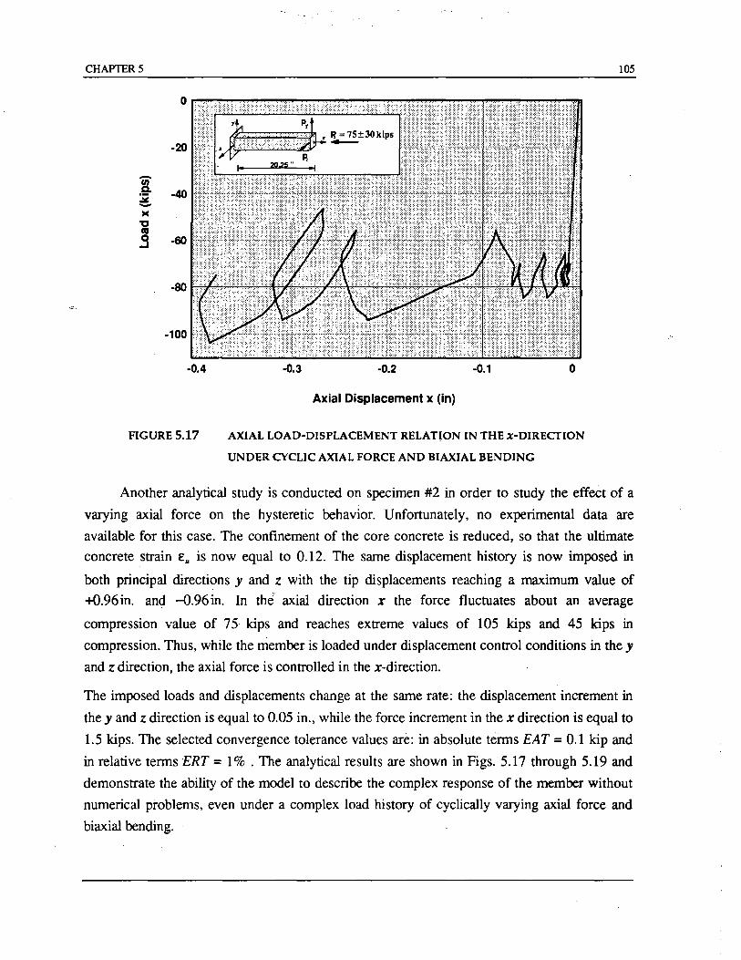
CHAPTERS
-20
J -40 ~ ->< 'C cu .9 -60
-80
-0.4
FIGURE 5.17
-0.3 -0.2 -0.1 o
Axial Displacement x (in)
AXIAL LOAD-DISPLACEMENT RELATION IN THE x-DIREcrION
UNDER CYCLIC AXIAL FORCE AND BIAXIAL BENDING
105
Another analytical study is conducted on specimen #2 in order to study the effect of a
varying axial force on the hysteretic behavior. Unfortunately, no experimental data are
available for this case. The confinement of the core concrete is reduced, so that the ultimate
concrete strain E" is now equal to 0.12. The same displacement history is now imposed in
both principal directions y and z with the tip displacements reaching a maximum value of
+0.96 in. and -0.96 in. In theC axial direction x the force fluctuates about an average
compression value of 75 kips and reaches extreme values of 105 kips and 45 kips in
compression. Thus, while the member is loaded under displacement control conditions in the y
and z direction, the axial force is controlled in the x-direction.
The imposed loads and displacements change at the same rate: the displacement increment in
the y and z direction is equal to 0.05 in., while the force increment in the x direction is equal to
1.5 kips. The selected convergence tolerance values are: in absolute terms EAT = 0.1 kip and
in relative terms ERT = 1 % . The analytical results are shown in Figs. 5.17 through 5.19 and
demonstrate the ability of the model to describe the complex response of the member without
numerical problems, even under a complex load history of cyclically varying axial force and
biaxial bending.
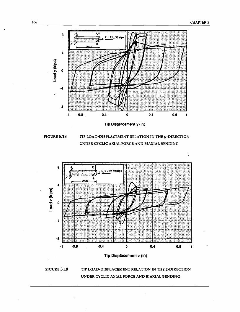
106
8
4
-rn a. ~ >- 0 '0
8 .... -4
-1
FIGURE 5.18
8
4 -.~ JIC -N "tJ 0 as 0
...J
-4
-8
-1
FIGURE 5.19
CHAPTER 5
-0.8 -0.4 o 0.4 0.8 1
-0.8
Tip Displacement y (in)
TIP LOAD-DISPLACEMENT RELATION IN THE y-DIRECTION
UNDER CYCLIC AXIAL FORCE AND BIAXIAL BENDING
-0.4 o 0.4 0.8
Tip Displacement z (in)
TIP LOAD-DISPLACEMENT RELATION IN THE z-DlRECTION
UNDER CYCLIC AXIAL FORCE AND BIAXIAL BENDING
1
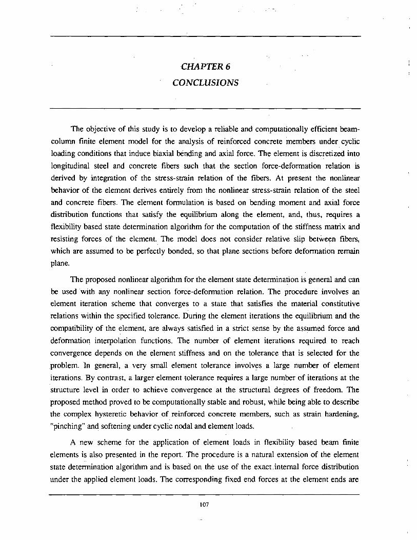
CHAPTER 6
CONCLUSIONS
The objective of this study is to develop a reliable and computationally efficient beam
column finite element model for the analysis of reinforced concrete members under cyclic
loading conditions that induce biaxial bending and axial force. The element is discretized into
longitudinal steel and concrete fibers such that the section force-deformation relation is
derived by integration of the stress-strain relation of the fibers. At present the nonlinear
behavior of the element derives entirely from the nonlinear stress-strain relation of the steel
and concrete fibers. The element fonnulation is based on bending moment and axial force
distribution functions that satisfy the equilibrium along the element, and, thus, requires a
flexibility based state determination algorithm for the computation of the stiffness matrix and
resisting forces of the element. The model does not consider relative slip between fibers,
which are assumed to be perfectly bonded, so that plane sections before deformation remain
plane.
The proposed nonlinear algorithm for the element state detennination is general and can
be used with any nonlinear section force-defonnation relation. The procedure involves an
element iteration scheme that converges to a state that satisfies the material constitutive
relations within the specified tolerance. During the element iterations the equilibrium and the
compatibility of the element, are always satisfied in a strict sense by the assumed force and
deformation interpolation functions. The number of element iterations required to reach
convergence depends on the element stiffness and on the tolerance that is selected for the
problem. In general, a very small element tolerance involves a large number of element
iterations. By contrast, a larger element tolerance requires a large number of iterations at the
structure level in order to achieve convergence at the structural degrees of freedom. The
proposed method proved to be computationally stable and robust, while being able to describe
the complex hysteretic behavior of reinforced concrete members, such as strain hardening,
"pinching" and softening under cyclic nodal and element loads.
A new scheme for the application of element loads in flexibility based beam finite
elements is also presented in the report. The procedure is a natural extension of the element
state determination algorithm and is based on the use of the exacUntemal force distribution
under the applied element loads. The corresponding fixed end forces at the element ends are
107
108 CHAPTER 6
determined during iterations of the element state determination. The presence of element loads
is important in the study of the effect of gravity loads on structures undergoing lateral load
reversals.
Compared with similar stiffness based beam-column elements, the proposed model
offers three major advantages: (a) with the use of the exact force distribution function along
the element fewer elements are needed to discretize a structure, (b) element softening can be
dealt with without numerical difficulties, and, (c) the application of element loads is rather
straightforward with the use of the exact internal force distribution function under the given
element loads. The element belongs to the family of flexibility based elements, but
distinguishes itself by the general and clearly formulated state determination process that relies
on the same equilibrium and compatibility conditions used in the formulation of the element
stiffnes~ matrix ,and does not resort to ad hoc approximations and special solution strategies to
avoid numerical difficulties. Compared with fiber beam-column elements that are based on the
event-to-event solution scheme, the proposed model is more general, since it is not limited to
piecewise linear force-deformation relations. It is also more efficient in the analysis of large
structures that may experience a very large number of events during severe cyclic loading,
since it does not require tracing of every stiffness change in the structure.
Comparisons between the results of the proposed model with experimental data show
very good correlation,especially, for cycles that induce small to average damage in the
members under investigation. Since the shear deformations are not included in the proposed
beam-column element, the selection of specimens for testing the validity of the model is
limited to cases with negligible contribution of shear deformations to the overall response.
Under very large inelastic deformations the model exhibits higher resisting forces than those
measured in the experiment. This is predictable, since the model does not include several
important effects in the material models of the constituent fibers, such as the effect of C;yclic
damage on the unconfined and confined concrete response, the buckling of the longitudinal
reinforcing bars and the effect of shear and bond-slip of reinforcing bars on the state of
damage of the member. Moreover, the model does not account for the fixed end rotation due
to reinforcing bar pull-out from the base of the specimen. Under imposed displacement
conditions the bar pull-out has a slight effect on the load carrying capacity of the specimen,
but it affects significantly the ,reloading stiffness and the energy dissipation capacity of the
specimen.
The proposed element that is now clearly formulated and implemented in the stand
alone computer program BEAMCOL offers several opportunities for future studies:
CHAPTER 6 109
• The effect of more sophisticated material models for unconfined and confined concrete
as well as for reinforcing steel on the local and global hysteretic response of reinforced
concrete members needs to be studied. The present study is limited to rather simple
constitutive models,' which lack important features, such as the effect of cyclic damage
on the concrete stress-strain relation, the buckling of reinforcing steel, etc.
• Parametric studies are required to establish the sensitivity of the element response to the
number of integration points (control sections) in the member. The case studies in this
report are conducted under displacement control and show that; while the load
displacement response is well represented with as few as 3 integration points, the section
moment-curvature response is very sensitive to the number of integration points. This
has very important practical ramifications, since it is the local response, such as steel and
concrete strains at the most critical section, that will detennine the failure of the element.
Thus, modeling guidelines are needed for the selection of the number of integration
points in order to predict with confidence curvature and rotation ductility demands and
plastic hinge lengths in reinforced concrete members.
• Second order effects, such as those arising from P-.6. actions, should be included in the
element in order to study the importance of overturning moments under the large lateral
sways caused by strong ground motions.
• The effect of fixed end rotations due to reinforcing bar pull-out from foundations and
bearn-column joints should be included in the model by modification of the behavior of
the end sections or by the addition of special hinge elements at the beam ends.
• The reinforcing bar slip relative to concrete is also important along the element,
particularly, for members with insufficient development length, lap splices, etc. The
rational inclusion of this effect in the section constitutive relation is a challenging task
that requires further study.
• The proposed element does not account for deformations due to shear and torsion. It is
presently not clear whether these effects can be included in a rational way in a fiber
beam-column element, but the subject merits further study.
• The proposed element enhanc.ed with the new method for the inclusion of element loads
is suitable for the analysis of prestressed concrete members. These can be modeled as a
group of prestressing tendons that are connected in parallel with the proposed reinforced
concrete beam-column element. Such an element is the subject of a current study.
• The proposed nonlinear solution algorithm is generally applicable. Its implementation in
110 CHAPTER 6
elements with different nonlinear section force-defonnation relations should be explored.
Similarly, the extension of the algorithm to systems that are composed of a combination
of several springs in series and/or in parallel should be studied.
• The implementation of the proposed beam-column element in a general fmite element
computer program for the nonlinear static and dynamic analysis of large structures is a
very important task. The implementation of the element in the finite element program
FEAP is presently complete. It is . only briefly discussed in this study and will be the
subject of a future report. Topics to be addressed in this future study include parametric
studies for the development of modeling guidelines for the nonlinear analysis of
reinforced and prestressed concrete structures under earthquake excitations and the
exploration of different nonlinear solution strategies within the framework of program
FEAP.
• Starting from the existing capabilities of the finite element program FEAP with respect
to nonlinear solution strategies and pre- and post-processing utilities, an integrated
computer environment for the nonlinear static and dynamic analysis of reinforced and
prestressed concrete structures needs to be developed .. This analysis package should
encompass elements with different levels of complexity, from simple linear elastic
elements to very sophisticated nonlinear 3-D finite elements, and should allow for their
seamless integration within the same nonlinear structural model.
REFERENCES
Anagnostopoulos, S. (1981). "Inelastic Beams for Seismic Analysis of Structures." Journal of Structural Engineering, ASCE, 107(ST7), pp. 1297-1311.
Banon, H., Biggs, J. and Irvine, M. (1981). "Seismic Damage in Reinforced Concrete Frames." Journal of Structural Engineering, ASCE, 107(ST9), pp. 1711-1729.
Bazant, S. and Bhat, P. (1977). "Prediction of Hysteresis in Reinforced Concrete Members." Journal of Structural Engineering, ASCE, 103(STl), pp. 151-167.
Bertero, V.V., Aktan, A., Charney, F. and Sause, R. (1984). "Earthquake Simulator Tests and Associated Experimental, Analytical and Correlation Studies of One-Fifth Scale Model." in, Earthquake Effects on Reinforced Concrete Structures, American Concrete Institute, SP-84-13, Detroit, pp. 375-424.
Brancaleoni, F., Ciampi, V. and Di Antonio, R. (1983). "Rate-Type Models for Non Linear Hysteretic Structural Behavior." EUROMECfl Colloquium, Palermo, Italy.
Charney, F. and Benero, V.V. (1982). "An Evaluation of the Design and Analytical Seismic Response of a Seven Story Reinforced Concrete Frame-Wall Structure." Report EERC 82-08, Earthquake Engineering. Research Center, Berkeley:
Chen, W. and Atsuta, T. (1977). Theory of Beam-Columns. McGraw Hill, New York.
Ciampi, V. and Carlesimo, L. (1986). "A Nonlinear Beam element for Seismic Analysis of Structures." 8th European Conference on Earthquake Engineering, Lisbon.
Ciampi, V. and Nicoletti, M. (1986). "Parameter Identific,!tion for Cyclic Constitutive Models with Stiffness and Strength Degradation." 8th European Conference on Earthquake Engineering, Lisbon.
Clough, R. and Benuska, L. (1967). "Nonlinear Earthquake Behavior of Tall Buildings." Journal of Mechanical Engineering, ASCE, 93(EM 3), pp. 129-146.
Clough, R. and Johnston, S. (1966). "Effect of Stiffness Degradation on Earthquake Ductility Requirements." Transactions of Japan Earthquake Engineering Symposium, Tokyo, pp. 195-198. .
Darvall, L.P. and Mendis, P. (1985). "Elastic-Plastic-Softening Analysis of Plane Frames." Journal of Structural Engineering, ASCE, 11 (ST4), pp. 871-888.
Filippou, F.C., Popov, E.P. and Bertero, V.V. (1983). "Effecl~ of Bond Deterioration on Hysteretic Behavior of Reinforced Concrete Joints." EERC Report 83-19~ Earthquake Engineering. Research Ceriter, Berkeley.
Filippou, F.C., and Issa, A. (1988). "Nonlinear Analysis of Reinforced Concrete Frames under Cyclic Load Reversals." EERC Report 88-12, Earthquake Engineering. Research Center, Berkeley.
Giberson, M. (1967). "The Response of Nonlinear Multi-Story Structures SUbjected to Earthquake Excitations." Earthquake Engineering Research Laboratory, Pasadena.
Hellesland, 1. and Scordelis, A. (1981). "Analysis of RC Bridge Columns Under Imposed Defonnations." IABSE Colloquium, Delft, Netherlands, pp. 545-559.
Iwan, W. (1978). "Application of Nonlinear Analysis Techniques." in, Iwan W. ed., Applied Mechanics in Earthquake Engineering, ASME, AMD, 8, New York, pp. 135-161.
Kaba, S. and Mahin, S.A. (1984). "Refined Modeling of Reinforced Concrete Columns for Seismic Analysis." EERC Report 84-03, Earthquake Engineering Research Center, University of California, Berkeley.
Karsan, I.D., and Jirsa, J.O. (1969). "Behavior of Concrete under Compressive Loadings", Journal of the Structural Division, ASCE, 95(STl2).
Kent, D.C. (1969). "Inelastic Behavior of Reinforced Concrete Members with Cyclic Loading.". Ph.D. Thesis,
111
112 REFERENCES
University of Canterbury, Christchurch, New Zealand.
Kent, D.C., and Park, R. (1971). "Flexural Members with Confined Concrete", Journal of the Structural Division, ASCE, 97(ST7).
Keshavanian, M. and Schnobrich, W. (1985). "Inelastic Analysis of RC Coupled Shear Walls." Earthquake Engineering and Structural Dynamics, 13. pp. 427-448. ,-
Lai, S., Will, G. and Otani, S. (1984). "Model for Inelastic Biaxial Bending of Concrete Members." Journal of Structural Engineering, ASCE, I IO(STl1), pp. 2563-2584.
Low, S.S. and Moehle J.P. (1987). "Experimental Study of Reinforced Concrete Columns Subjected to MuItiAxial Cyclic Loading.'! EERC Report 87-14, Earthquake Engineering Research Center, University of California, Berkeley.
Ma, S.Y., Bertero, V.V. and Popov, E.P. (1976). "Experimental and Analytical Studies on the Hysteretic Behavior of Reinforced Concrete Rectangular and T-Beams", EERC· Report 76-2, Earthquake Engineering Research Center, University of California, Berkeley.
Mahasuverachai, M. (1982). "Inelastic Analysis of Piping and Tubular Structures." EERC Report 82-27; Earthquake Engineering Research Center, University of California, Berkeley. .
Mander, 1.B., Priestley, M.l.N. and Park, R. (1988). "Theoretical Stress-Strain Model for Confined Concrete." Journal of Structural Engineering, ASCE, 114(ST8), pp. 1804-1826. ,
Mari, A. and Scordelis, A. (1984). "Nonlinear Geometric Material and Time Dependent Analysis of Three Dimensional Reinforced and Prestressed Concrete Frames." SESM Report 82-12, Department of Civil Engineering, University of California, Berkeley.
Menegotto M., and Pinto, P.E. (1973). "Method of Analysis for Cyclically Loaded Reinforced Concrete Plane Frames Including Changes in Geometry and Non-Elastic Behavior of Elements under Combined Normal Force and Bending", Proceedings. IABSE Symposium on Resistance and Ultimate Deformability of Structures Acted on by Well Defined Repeated Loads", Lisbon, pp. 15-22.
Menegouo, M. and Pinto, P.E. (1977). "SlenderRC Compressed Members in Biaxial Bending." Journal of 'Structural Engineering, ASCE, 103(ST3), pp. 587-605.
Meyer, c., Roufaiel, M.S. and Arzoumanidis, S.G. (1983). "Analysis of Damaged <;:oncrete Frames for Cyclic Loads." Earthquake Engineering and Structural Dynamics. Vol. 11. pp. 207-228.
Okada, T., Seki, M. and Asai, S. (1976). "Response of Reinforced Concrete Columns to Bi-directional Horizontal Forces and Constant Axial Force." Bulletin ofERS, 10, Tokyo, pp. 30-36.
Otani, S. (1974). "Inelastic Analysis of RIC Frame Structures." Journal of the Structural Division, ASCE, l00(STI).
Ozdemir, H., (1981). "Nonlinear Transient Dynamic Analysis of Yielding Structures." Ph. D. Thesis, Department of Civil Engineering, University of California, Berkeley.
Prager, W. and Hodge, P. (1951). Theory of Perfectly Plastic Solids, lohn Wiley and Sons, New York.
Roufaiel, M.S.L. and Meyer, C. (1987). "Analytical Modeling of Hysteretic Behavior of RIC Frames." Journal of Structural Engineering, ASCE. 113 (ST3), pp. 429-444.
ScoU, B.D., Park, R. and Priestley, M.l.N. (1982). "Stress-Strain Behavior of Concrete Confined by Overlapping Hoops at Low and High Strain Rates", ACI Journal. Vol. 79. No.1, pp. 13-27.
Sheikh, S. and Yeh, C.c. (1990). "Tied Concrete Columns Under Axial Load and Flexure." Journal of Structural Engineering, ASCE. 1.16 (STIO), pp. 2780-2800.
Soleimani, D., Popov, E.P. and Bertero, V.V. (1979). "Nonlinear Beam Model for RIC Frame Analysis." 7th ASCE Conference on Electronic Computation. St. Louis.
Spacone, E., Ciampi, V. and Filippou, F.C. (1992). "A Beam Element for Seismic Damage Analysis." EERC Report, to be published, Earthquake Engineering Research Center, University of California. Berkeley.
Takayanagi, T. and Schnobrich, W. (1979). "Non Linear Analysis of Coupled Wall Systems." Earthquake Engineering and Structural Dynamics, Vol. 7, pp. 1-22
Takeda, T., Sozen, M.A. and Nielsen, N. (1970). "Reinforced Concrete Response to Simulated Earthquakes."
_R_EF_E_R_EN_C_~ _______________________________________________________ 1~131IJY
Journal of Structural Engineering, ASCE, 96(STl2), pp. 2557-2573.
Takizawa, H. (1976). "Notes on Some Basic Problems in Inelastic Analysis of Planar RC Structures." , Trans. of Arch. Inst. of Japan, 240, Part I in Feb. 1976, pp. 51-62, Part II in March 1976, pp. 65-77.
Takizawa. H. and Aoyama, H. (1976). "Biaxial Effects in Modeling Earthquake Response of RC Structures." Earthquake Engineering and Structural Dynamics, 4, pp. 523-552.
Zeris. c.A. (1986). "Three Dimensional Nonlinear Response of Reinforced Concrete Buildings." Ph. D. Thesis, University of California, Department of Civil Engineering, Berkeley.
Zeris, C.A. and Mahin, S.A. (1988). "Analysis of Reinforced Concrete Beam-Columns under Uniaxial Excitation." Journal of Structural Engineering, ASCE, 114(ST4), pp. 804-820.
Zeris, c.A. and Mahin, S.A. (1991). "Behavior of Reinforced Concrete Structures SUbjected to Biaxial Excitation." Journal of Structural Engineering, ASCE, 117(ST9), pp. 2657 -2673.
Zienkiewicz, O.c. and Taylor, RL. (1989). The Finite Element Method. Volume 1. Basic Formulation and Linear Problems. Fourth Edition. McGraw Hill. London.
Zienkiewicz. O.C. and Taylor. R.L. (1991). The Finite Element Method. Volume 2. Solid and Fluid Mechanics. Dynamics and Non-Linearity. Fourth Edition. McGraw Hill. London.

APPENDIX A
SUMMARY OF SOLUTION ALGORITHM
The numerical procedure for the stand alone computer program is summarized here in a
series of steps that parallel those at the end of Chapters 2 and 3. While the summaries at the
end of Chapters 2 and 3 were limited to a basic description of the sequence of steps for the
sake of clarity, this appendix contains the detailed numerical implementation of the procedure
with the state of each variable within the nested iteration process denoted by superscripts
according to the notation introduced in Section 4.2. The steps of the algorithm are also
illustrated in Figs. A.I-A.4:
(1) Start the analysis.
Setk=1
(2) Start the Newton-Raphson iterations.
Set i=1.
(3) Solve the global system of equations and update the structure displacement increments.
Using the unbalanced force vector (p~y-l and the structure tangent stiffness matrix
(K!)i-l from the previous Newton-Raphson iteration i-1, the change in the structure
displacement increments (06pk r is computed from the solution of the linear system of
equations
(A. I)
The unbalanced force vector (p~ y-l is obtained as the difference between total applied
loads and total resisting forces at the conclusion of the previous Newton-Raphson
iteration i-1 in step (19). When k=1 and i=1, (p~ t = 6Pi. The tangent stiffness matrix
(K!y-I is based on the state of the structure at the end of the previous Newton-Raphson
iteration and is detennined in step (18). When i=1, two alternatives exist:
k= 1.' The initial tangent stiffness K~ is detennined by imposing a very small
defonnation increment on the sections ()f all elements. The fiber material modules
return the initial tangent modulus of elasticity Era" from which the section, element
and, finally, the structure stiffness is assembled. For the proposed concrete model,
115
116 APPENDIX A
which has zero stiffness in tension, the initial tangent modulus always corresponds
to the initial tangent stiffness in compression.
k> 1: The structure stiffness is equal to the tangent stiffness at the end of the last load
step k-1, that is (K:t = K:-I;
The structure displacement increments (O~pky are added to the displacement increments i-I-
(~pk) at the end of the previous Newton-Raphson iteration i-I to obtain the
displacement increment (~pk r for iteration i.
(~pkr = (~pkrl +(o~pkr (A.2)
When i=1, (~pk)O is initialized to zero.
(4) Compute the element deformation increments.
Using the compatibility matrix L e1e the change in the element deformation increments
(Otll/)i is computed from the structure displacement increments (O~pky:
(A.3)
The element deformation increments are updated for iteration i:,
(A.4)
When i= 1, (&/ t is initialized to zero. Note that the element displacement increments
do not change during the element iteration loop j.
(5) Start the element state determination.
Setj=1.
(6) Compute the change in the elementforce increments.
Two cases are possible:
j=1: ((O~Qinl is obtained from the change in the element displacement increments
(o~'l Y for the current Newton-Raphson iteration i using the element tangent
stiffness matrix (Ki(1 at the end of Newton-Raphson iteration i-1
(A.5)
j>1: ((O~Qirr is obtained from the residual element deformations ((lry-I at the end
of iteration j-/ and the corresponding element stiffness matrix
APPENDIX A 117
(A6)
(7) Update the elementforce increments and the element resisting forces.
With the change in the element force increments ((o~Qtyr, the element force
increments (( ~Qk r r1
are updated for iteration):
(A.7)
o When i=1 and}=], ((~Qt)l) is initialized to zero.
The current element resisting forces are obtained by adding the element force increments
to the resisting force vector QH at the end of the converged load step k-]:
(A8)
(8) Compute the section force increments ..
The change in the section force increments is computed with the interpolation function
b(x) and the corresponding force increments are updated
((om\X)rr = b(X),((o~Qtrr
((MJt(X)rr = ((mk(x)y)j-l + ((OMJt(X)nj
o When i=1 and}=], ((MJt(x)n is initialized to zero.
Update the current section forces
When k=1, Dt-1(x) = O.
(9) Compute the change in section deformation increments.
(A.9)
(A 10)
(All)
The change in section deformation increments (( o~dt (x) r r is obtained by adding the
effect of the change in section force increments ((omt(X)yr to the residual section
deformations at the end of the }-1 iteration:
(AI2)
118 APPENDIX A
The section defonnation increments are then updated:
(A. 13)
o When i=1 and)=1, ((~dl:(x)r) = O.
(10) Compute the fiber deforma"tion increments.
The change in fiber defonnation increments is computed with the section compatibility
matrix lex) and the defonnation increments are updated
((06tl(x)rY =1(x)'((OMI:(x)rY
((~el:(x)rr = ((6el:(X)r(1 + ((o~k(X)rr
The fiber defonnations are updated:
o When i=1 and)=1, ((~ek(x)n = O.
(11) Compute fiber stresses and update the tangent modulus of the fibers.
(A. 14)
(A.15)
(A.16)
For the current fiber deformations ((ek(X)rY the fiber material modules return the new " J
fiber stresses ((Ek(x'Yi/ib,Zifib»)') and the updated tangent stiffness modulus of the fibers
((E!II(X'Yifib,lifib)y)J.
(12) Compute the section tangent stiffness and flexibility matrices.
i J The updated tangent modulus of the fibers (( E1: II (x, Yifib' Zifib»)) is used in the calculation
of the current section tangent stiffness matrix
11(:»
L (EA )ifLb . Yi~b ifib=1
11(:»
- L(EA)iflb . Yifib' lifib iflb=l
11('>:)
- L,(EA)iflb . Yifib iflb=l
11(:»
- L (EA)ifib' Yifib' Zifib ifib=l
11(:»
L(EA)ifib . Z~b ifib=l 11(:»
L(EA)ifib' Zi/ib ifib=1
11('>:)
- L(EA)i/ib' Yiflb ifib=l
11('>:)
L(EA)ifib'lifib ifib=l
11(:»
L(EA)ifib ifib=l
(A.17)
APPENDIX A 119
with
n(x) is the total number of fibers in the section. The section stiffness matrix is then
inverted to yield the current section flexibility matrix:
(A.18)
(13) Compute the section resisting forces.
The section resisting forces are determined from equilibrium between the fiber stresses , j
(( ak (x, Yijib' Zi/ib) n and the section resisting forces .
.. (x) , j
- I((ak(x'Yi/ib,Zi/ib»)'} . Aijib · Yijib ijib=!
.. (x) , j
I((ak(x'Yijib,Zijib»)'} . Ai/ib' Zijib ijib=l
.. (x) , j
I((ak(x'Yi/ib,Zi/ib»)'} . Ai/ib ijib=l
(14) Compute the section unbalancedforces.
(A.19)
The section un balanced forces are the difference between applied loads and resisting
forces:
(A.20)
Check whether the unbalanced force vector satisfies the specified section tolerance.
(15) Compute the residual section deformations.
(A.21)
(16) Compute the element flexibility and stiffness matrices.
The element flexibility matrix is obtained by numerical integration of section flexibilities:
(A. 22)
where m is the number of monitored sections in the beam-column element x .. scc the x
coordinate of the section in the local reference system and w/lSCC the corresponding
weight factor. The element stiffness matrix is obtained by inverting the flexibility matrix.
120 APPENDIX A
. (A.23) _
(17) Checkfor element convergence.
Element convergence is achieved when all section unbalanced forces satisfy the specified
section tolerance. Two cases are possible:
a) If convergence is achieved go to step (18)
b) If convergence is not achieved then compute the residual element deformations
(A. 24)
incrementj by 1 and return to step (6).
(18) Compute the structure resisting forces and update thestructure stiffness matrix.
When all elements have converged, the i-th Newton-Raphson iteration is complete. The
structure resisting forces (p;r are detennined by assembly of all element resisting forces
(Qk )i according to the expression .1.
(p; r = I L:I • . (Qk t. (A.25) .1.=1
The structure tangent stiffness matrix is updated by assembly of the element stiffness
matrices:
(Kk)i - ~ LT (Kk)i L s - £.J .1.' .1.·.1e (A.26)
.1.=1
(19) Compute the structure unbalancedforces.
The structure unbalanced forces (p~ r are the difference between total applied loads p; and total resisting forces (p; r :
(A. 27)
where P; is detennined from the total applied load at the en'd of load step k-J and-the
current load increment
(A.28)
For k=] P~ = O.
(20) Checkfor structure convergence.
If the unbalanced forces at the structure level satisfy the specified tolerance,·
APPENDlXA 121
convergence is achieved. Correspondingly, two cases are possible:
a) If convergence is not achieved, increment i by 1, return to step (3) and stan the next Newton-Raphson iteration;
b)· If convergence is achieved, load step k is complete. Go to step (21).
(21) Update force and deformation vectors and start new load step.
All force and deformation vectors are updated by adding the vector increments for load
step k to the corresponding total forces and deformations at the end of load step k-l:
pk = pH +~pk
qk(X) = qk-I(X)':" ~qk(X)
dk(x) = dt-J (x) + Mk(X)
update Et-J(x) to Ek(X)
ek (x) = et-J(x) + ~ek(x)
At this point, two cases are possible:
a) k=kn. The entire external load PE was applied and the analysis is complete.
b) k<kn. Increment k by l. Compute the new structure unbalanced force vector
(p~t = p: - p;-I
and return to step (2)
(A. 29)
(A. 30)
(A.31)
(A. 32)
. (A.33)
This summary refers to the stand alone implementation of the fiber beam-column
element and differs in several points from the implementation in program FEAP. The updating
of the variables in program FEAP follows more closely the summaries in Sections 2.5 and 3.6
and the corresponding figures. The convergence criteria, both, at the element and at the
structural level are also different, as discussed in Chapter 4: the stand alone program checks
element convergence by monitoring the unbalanced section forces. Similarly, convergence at
the structure level is checked by monitoring the unbalanced forces at the global degrees of
freedom. In program FEAP, both, at the structure and at the element level convergence is
checked by monitoring the work increments. The latter method is more general and is
particularly suitable for structures near the ultimate load capacity, as discussed in Section 4.5.
The steps of the nonlinear solution algorithm are illustrated in. Figs. A.I-AA. Fig. A.I
depicts the load-displacement history at the structure level. The structure is subjected to three
load step increments ~p:. Three Newton-Raphson iterations are performed within each load
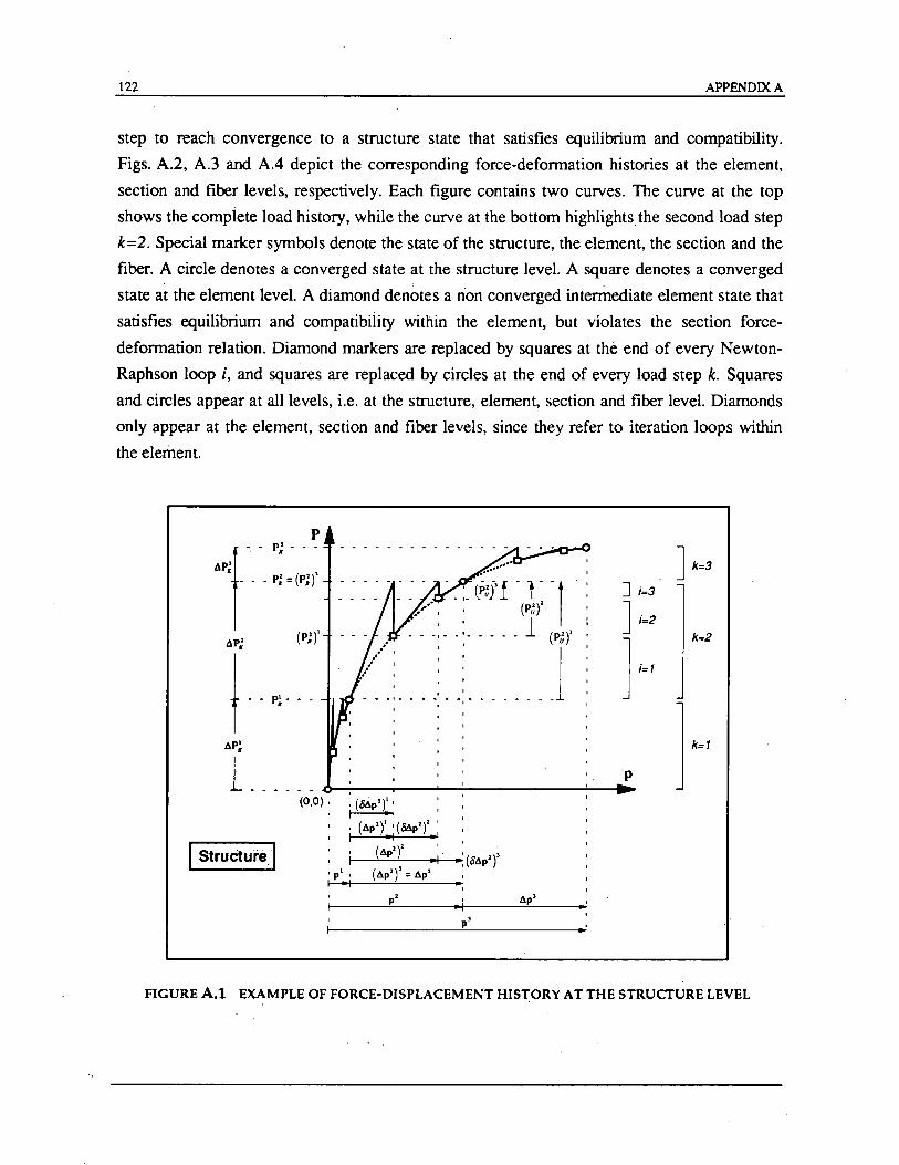
122 APPENDIX A
step to reach convergence to a structure state that satisfies equilibrium and compatibility.
Figs. A.2, A.3 and A.4 depict the corresponding force-deformation histories at the element,
section and fiber levels, respectively. Each figure contains two curves. The curve at the top
shows the compiete load history, while the curve at the bottom highlights the second load step
k=2. Special marker symbols denote the state of the structure, the element, the section and the
fiber. A circle denotes a converged state at the structure level. A square denotes a converged
state at the element level. A diamond denotes a non converged intermediate element state that
satisfies equilibrium and compatibility within the element, but violates the section force
deformation relation. Diamond markers are replaced by squares at the end of every Newton
Raphson loop i, and squares are replaced by circles at the end of every load step k. Squares
and circles appear at all levels, i.e. at the structure, element, section and fiber level. Diamonds
only appear at the element, section and fiber levels, since they refer to iteration loops within
the element.
-:- cP~5' f - t - -1 .' " (P~)'
" 1 • - - -, - -' - - - - - (P~)'
./' :: 1 .... I I I
'- - -: - - - -: - -: - - - - - - - -
] i=3
] i=2
] ,=,
1 ______ ~....----'--~-----:......~ (0,0) , : (.5,ip')' , ~
p
. (6p')' '(&1p')' , I ·1 .'
(&p')' .; .: (.56p')' 'p', (6p')' = 6p' 1 .1 .. ,
I· Structure I p' 6p'
• p'
] k=3
k=2
l·=,
FIGURE A.I EXAMPLE OF FORCE-DISPLACEMENT HISTORY AT THE STRUCTURE LEVEL
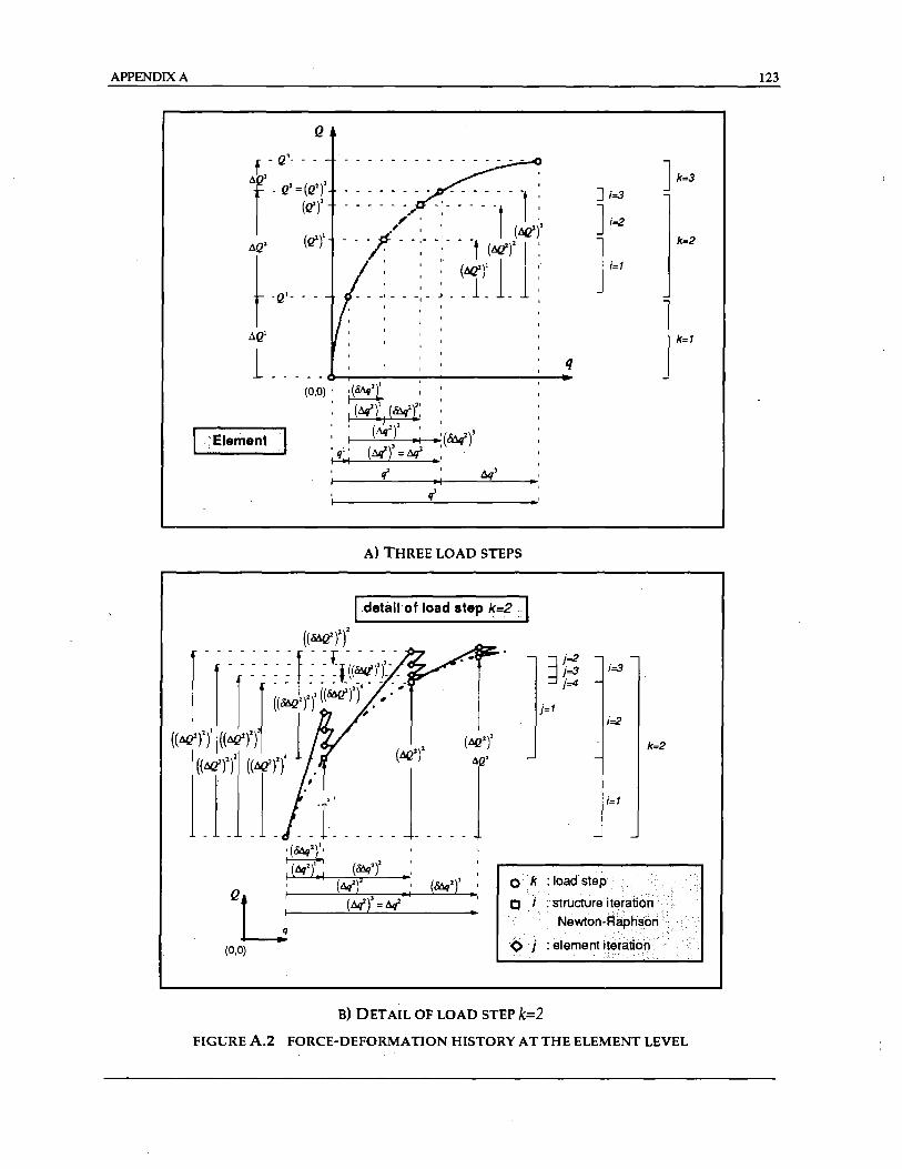
APPENDIX A
Q
·Element
'1
. '
A) THREE LOAD STEPS
I detail of load step k=2 •• 1
((MQ')')'
;=3 [- -: I ~ ~ Un· «j~t:(~ (( ""')')'((""')'I~ 1 ' , I"<!')'
j((.xf)')j ((.xr)')'. (~ ) AQ'
~ j=2 j=3 j=4
j=1 ;=2
J J -'r ---J ----1 ;(Mq'~; ( ')' (0&1)' .' I &i. I _
, (&It .; ,
(Mq'j' , . ,
(0,0)
Ok: Joadstep
01 :structureiteratlon NeWton~R~hson
<> j :elementitElration·· ...
B) DETAIL OF LOAD STEP k=2
FIGURE A.2 FORCE-DEFORMATION HISTORY AT THE ELEMENT LEVEL
123
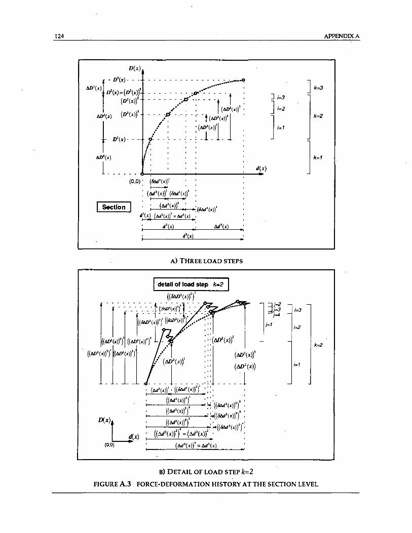
124
D(z)
f -D'(z) - - - - - - - - - - - - - - - - -•• ;."--"~
4D1(Z) 3 ......... I
Ii(z) = (Ii(z») - - - - - - - - .;r.r-" - - - - - + ' (D'(z»)' - - - - - - .-.d -, - - - -f I :
.- I I l ) ,'" (.w'(Z» ,
Mt'(Z) (D'(z») - -.">~~ -.- : -:-(J~~l(z»J • I I I 1
DI (z) - - - i- --'- -- ~ - ! - - -. , / .
] ;=3
] ;=2
lel
.w'(z) i : 1_ - - - - -O---:-,-_-~ d(z)
(0,0): (~Z(z»)' r---
: (~'(z»)' (~Z(~»Z ' 1 .1 .'
ISection :; (~Z(z»)'.: .:(8&1Z(~»J d'(z) (&I'(~))' = &1'(,,) , I -I - - •
d'(z) .1 ~)(z) . , d'(z) •
A) THREE LOAD STEPS
D(X)t
W(x) (0,0) (&/2(Z»)' = &/'(z) ..
B) DETAIL OF LOAD STEP k=2
r!~ }=3 j=4
j=1
J k=3
k=2
] kel
;=3
;=2
k=2
;=1
FIGURE A.3 FORCE-DEFORMATION HISTORY AT THE SEcrION LEVEL
APPENDIX A
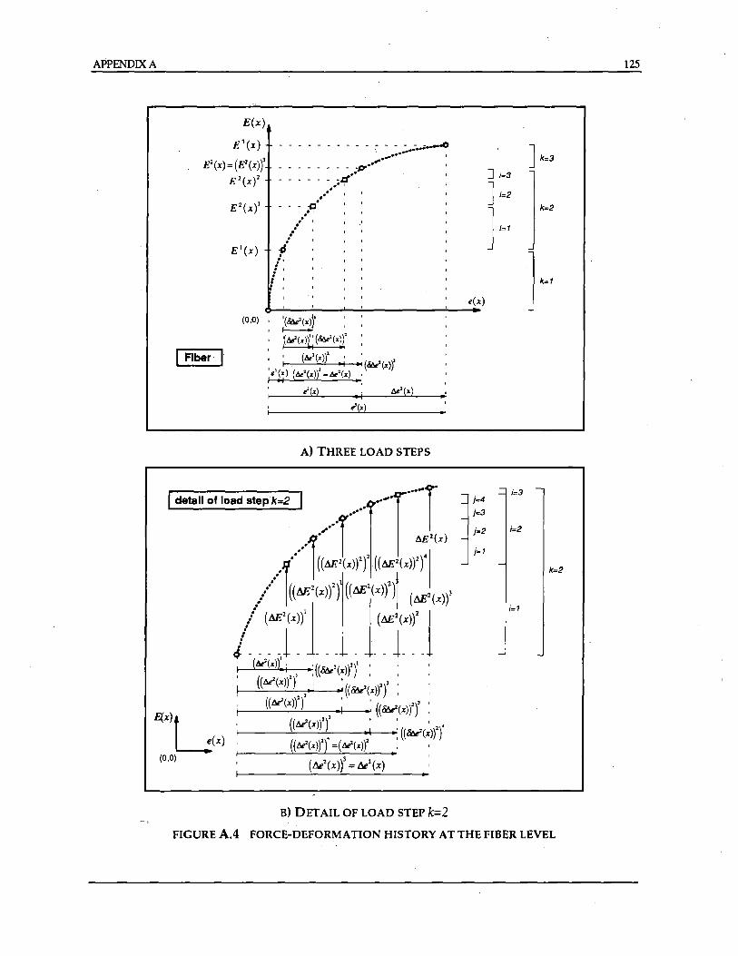
APPENDIX A
E(x)
E](x)
E2(X) = (E\x)Y E 2 (X)2
E2(X)'
E'(x)
- - - - - - - - - - - - - - - -.... .0 " .............. I
: : : : : : :~ •• -sr ..... .... : : ..
- - - .~. I I , , •••• I , .'
... i l' , ' . , : I '
, , , '
~ , , ,
(0,0) , '(&e2 (>:)l' I-'-------'
, ' , '
I Fiber·
~X)L e(X)
(0,0)
~M(X)i;(&e2(>:~2 ,
: ;. (6<2(:))' .; .: (&e'(>:))' ~'(x) (6<'(>:)) = &'(>:) ,
, ., II I
e'(X) • i &'(X)
..'(x)
A) THREE LOAD STEPS
B) DETAIL OF LOAD STEP k=2
] k=3
] ;=3
] i=2 k=2 l·,
e(x)
}.,
;=3
r i=3
j=2 ;=2
j=1
k=2
;=1
FIGURE A.4 FORCE-DEFORM A nON HISTORY AT THE FIBER LEVEL
125
126 APPENDIX A
It is important to nore that force and deformation vectors are not updated at the end of
every Newton-Raphson iteration when all elements have converged, but at the end of every
load step when convergence is reached at the structure level . The updating process is very
important for the fiber constitutive relations. The fiber resisting force and tangent modulus is computed based on the total strain at the previous converged load step £k-l (X"SClC' Yi/ib' zi/ib) and
the current total strain increment (( .1£k (X"SClC' Yqib' Zqib»)i t This procedure guarantees the path
independence of the nonlinear solution algorithm and has the advantage that in the case of
non-convergence the analysis can be restarted from the previous converged load step with a
smaller increment. The same updating procedure is used, both, in program FEAP and in the
stand alone program.
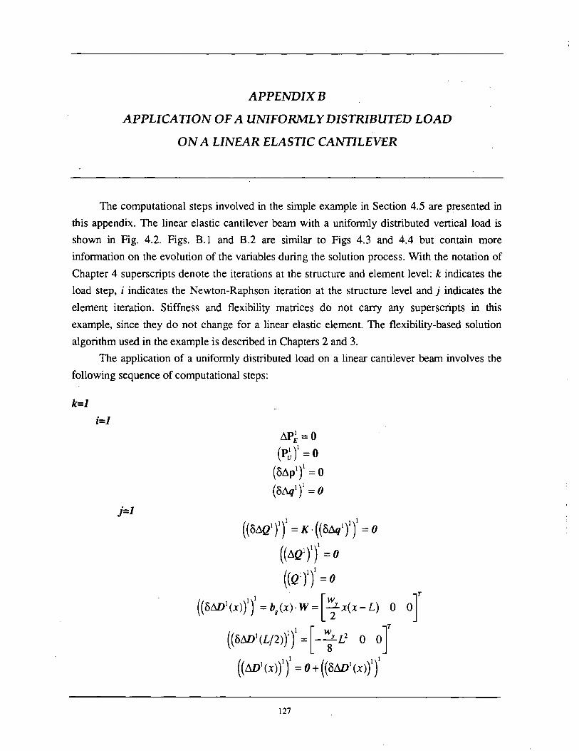
APPENDIXB
APPLICATION OF A UNIFORMLY DISTRIBUTED LOAD
ON A LINEAR ELASTIC CANTILEVER
The computational steps involved in the simple example in Section 4.5 are presented in
this appendix. The linear elastic cantilever beam with a uniformly distributed vertical load is
shown in Fig. 4.2. Figs. B.l and B.2 are similar to Figs 4.3 and 4.4 but contain more
information on the evolution of the variables during the solution process. With the notation of
Chapter 4 superscripts denote the iterations at the structure and element level: k indicates the
load step, i indicates the Newton-Raphson iteration at the structure level and j indicates the
element iteration. Stiffness and flexibility matrices do not carry any superscripts in this
example, since they do not change for a linear elastic element. The flexibility-based solution
algorithm used in the example is described in Chapters 2 and 3.
The application of a uniformly distributed load on a linear cantilever beam involves the
following sequence of computational steps:
k=1
;=1
j=1
t1pi = 0
{Pb f = 0
(Ot1pl r = 0
(0t1t/)1 = 0
((0t1Q1nl
= K.({0t1t/)I)1 =0
({t1QI)1 f = 0 1
({Qln = 0
((MD'(x))'f ;b,(X).w;[i x(x-L) 0 oJ ((MD'(L/2))')' ;[ - i L' 0 oJ
1 1
((Mi(x)n = 0+ ((OMi(x)f)
127
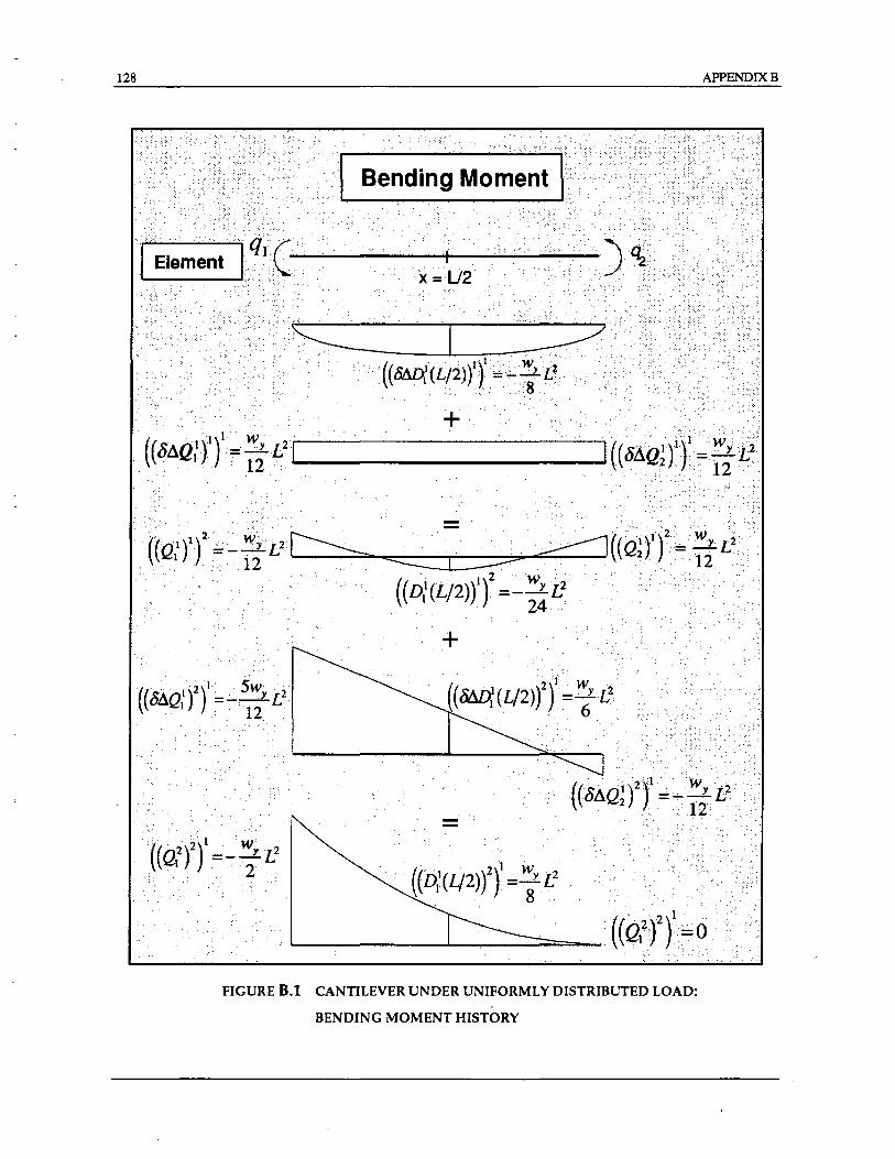
128 APPENDIXB
:, '.' ': .. :,,'
............ ( ......... .
E,ementlil( ...... ·.··.·~ .. :. ~~----------4-----~~...;..;,..;.-----
. : : ".; :<~;':.:' .~.:~.~ ",' .. :":
. ···((Qtt)'='-3: l.'c:-:--:--. .... .. .•. ... .. p--==1 ((~nl)',.W, Lt •.. .. ... .. 12 . . .... . c:::::::::::::: r :::::::::::="'" .. .. .... .... 12..: ..
. . ((D11(L/2)rt =~~;L2
+
FIGURE B.l CANTILEVER UNDER UNIFORMLY DISTRIBUTED LOAD:
BENDING MOMENT HISTORY
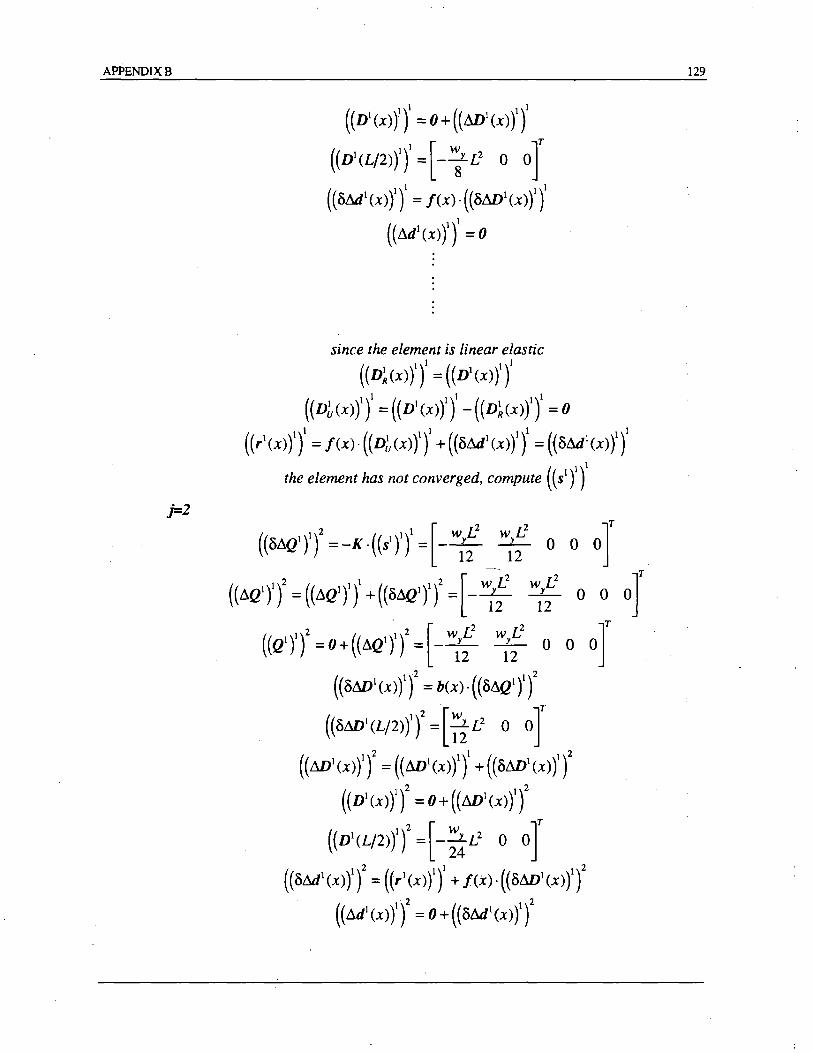
.APPENDIXB
j=2
1 ,
((Di(X»),} = O+((MJ'(X)Y)
((D'(L/2»)')' + '; L' 0 oJ ((SM'(X»)')' = f(X)-((SM)'(X)r)i
1
((!1d1(x»)I) =0
since the element is linear elastic
((D~(X)n' = ((Dl(X»)')'
((Db(X)y)i = ((Dl(X»),)1 _((D~(X»)')1 =0
((r 1(x)ff =f(X)-((Db(x)yf + ((SM'(x)f)' = ((SM1(x»)lf
the element has not converged, compute (( Sl Y f
129
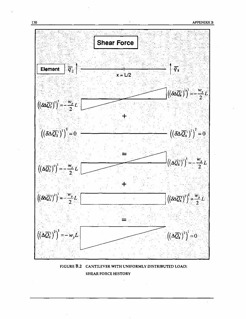
130 APPENDIXB
r'~':::~t~:;'fi:~2F-'-·'··· •. _ .. _.. -_ ........ ·•···· .......... ··.····.+-1 ..... ········---:· ........... ·· .. ·· ....... ···· ~ ............ .-;o.
·····~····~U2··
. ... . . . ..:...... ................... '
> ..•.. · .. ~ •.. ·····.i'.i ••. , ... i.'···.· .... '· .. : ...... . ....... Ii ·W\·· ....• .. . .....•... ~((~Qs') )~_u yL
~, .• ·i'· .. ·."" •..... :ii.>· .•.. i:1.'F
"", .'- " + .' ", .
.. ((&Qi t r.~ _li'YL. ··1·
.. ···2 . ...... ... .. '-----------------'
FIGURE B.2 CANTILEVER WITH UNIFORMLY DISTRIBUTED LOAD:
SHEAR FORCE HISTORY

APPENDIXB 131
since the element is linear elastic 2 2
((D~(x)n = ((D1(X)n 2
((Db(X)y) = 0
((rl(X)Y)2 =f(x)o((Db(X)y)1 =0
the element has converged
(Q1y=[_W/! wyI! 0 0 0 0 0 0 0 O]T. 12 12
(-1)1 (-1)1 [ wyI! WyL2 . wyL _ W2yL 0 0 o]T. Q = Q +lgoW= ---u- 12 0 0 0 --2-
j=J
( 1)1 _ - (-1)1 _[WyL2 WyL]T PR - L 0 Q - 12 -2.
(Pb f = pi -(PkY = 0- (Pk)1 = [_ WyL2 WyL]T 12 2
K 0 (OL\pl )2= (Pb )2 (L\pl t = (L\pl Y + (OL\pl)2 = 0 + (OL\pl)2
(&lql)2 = ~ o (&lpl)2 . (L\ql)~ = (L\ql Y + (OL\qI)2
1 - 1 [ 5w L2 W L2 ]T ((OL\Q1)2) = K o ((OL\qI)2) = ----rt- ---t2 0 0 0
((8Q')')' ~ (8Q')' + ((MQ')')' ~ [- w;L' 0 0 0 or 1 1 [ wI! ]T ((QI )2) = 0 +((L\QI )2) = -T 0 0 0 0
. 1 I
((OL\D1(X))2) = b(x)o((OL\Q1)2)
((O<W'(L/2))'j' ~[~ L' 0 or ((Mi(x»)2)1 = (W1(x)Y + ((OMi(x»)2)1
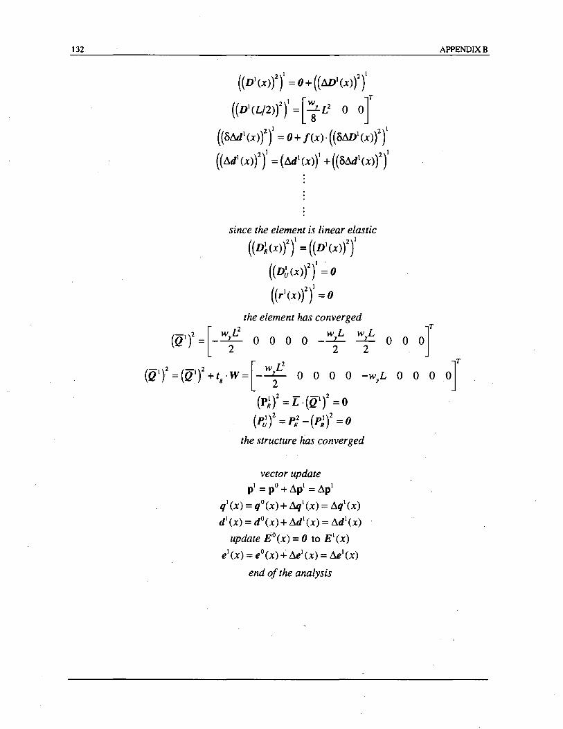
132
((D1(x)t)1 = 0+ ((Mi(x»)2f
((D'(L/2»)'f = [i L' 0 or ((orut(X})2f = 0+ f(x), ((OMi(x})2Y
((~dl(X»)2f = (M1(x)f + ((OM,(x»)2f
since the element is linear elastic
((D1(x»)2f = ((DI(X»)2y
((Db(X»)2f = 0
((rl(x»)2)1 = 0
the element has converged
(-1)2 [. W yL2 W L wyL Q = --- 0 0 0 0 --'1- --
2 2 2 o 0 oJ (-1)2 (-1)2 [ WyL2 Q = Q + 18 . W = --2- 0 0 0 0 -wyL 0 0 0
(p~)2 = L . (Q 1)2 = 0
( 1)2 2 ( 1)2 Pu = PE - PR =0
the structure has converged
vector update pi = po + ~pl = ~pl
ql(X) = qO(x)+ ~I(X) = ~ql(X) dl (x) = dO(x) + ~dl (x) = ~dl(X)
update EO(x) = 0 to EI(X)
el(x) = eO(x) + ~el(x) = ~1(X)
end of the analysis
APPENDIXB
APPENDIXC
APPLICATION OF SOLUTION ALGORITHM
TO A SIMPLE SOFTENING SYSTEM
The nonlinear solution algorithm for the element state determination is illustrated here
with the aid of the simple system of two extensional springs in series shown in. Fig. 4.5. One
spring is linear elastic, while the other is linear elastic-strain softening. As discussed in Chapter
4, the eqUilibrium and compatibility of the two spring system leads to the following relations:
Q=DA =Da
In this illustrative analysis a single deformation increment ~q is applied and the
corresponding resisting force increment ~Q is sought. Consequently, there is no need for the
use of superscripts k and i and only superscript j that describes the sequence of element
iterations is sufficient to represent the evolution of the system variables. Superscript i is only
used once to indicate that the element deformations are updated. Since the system is assumed
to be initially unstressed, the initial state is characterized by:
Qj=o = 0
d~ = d~ =0
f~ = fa.el
The steps for the nonlinear analysis of the two spring element are illustrated in Fig. 4.6. First,
133
134 APPENDIXC
the deformation increment /lq is imposed. This increment remains unchanged during the
iterations in order to satisfy the compatibility requirement. The total deformation of the
element is updated
qi=1 = qi=O + /lqi=1 = 0 + !lfJ = !lfJ
and the element iterations start:
j=1 Based on the initial element stiffness KO a first estimate of the element force increment
/lQI due to /lq is computed and the deformation increments caused by this force in the
extensionaL springs are determined:
i1.,i = f O ·ml A A A
Update the spring deformations and forces and determine the new spring flexibilities
d~ = d~ + M~ + r~ = /ld~
d l dO A...II' ° Ad l B = S + LlUB + rB = U B
i~ = is,pl
where rO are the initial residual deformations of the springs which are equal to zero. Compute the spring resisting forces D~ and D~ and the corresponding unbalanced
R R
forces:
D~ = D~ -D~ U R
, Compute the residual spring deformations rl and r~
APPENDIXC 135
j=2
rl =fl·Di =0 u
I J"I DI rB = JB' Bu
.~
Update the element flexibility and stiffness matrices:
FI - J"I +J"l - JA JB
Check for element convergence: spring B has a significant force unbalance, and,
consequently, the element has not converged. Compute the residual element deformation
Sl:
Start a new element iteration. With the residual element deformation at the end of the
previous iteration j=] compute the new element force increment
.1Q2 = -KI . Sl
Update the spring deformations and forces and determine the new spring flexibilities:
d~ = d~ + M~ + r~ = d~ + ~d~
d 2 dl A,/2 I B = B + LlUO + rB
Ii = IB,pl
Compute the spring resisting forces D~R and D~R and the corresponding unbalanced
136
forces:
D~ =D~ -D~ =0 U R
D~ = Di - DB2 = 0 U R
Compute the residual spring defonnations r;' and ri
r;' = 11· D~ = 0 U
ri =Ii .D~ =0 U
Update the element flexibility and stiffness matrices:
p2 =11 + Ii
APPENDIXC
Check for element convergence: both springs have zero force unbalance, and,
consequently, the element has converged and this simple analysis is complete.
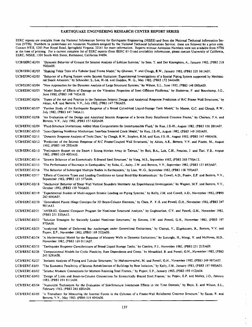
EARTHQUAKE ENGINEERING RESEARCH CENTER REPORT SERIES
EERC reports are available from the National Information Service for Eanhquake Engineering (NlSEE) and from the National Technical Information Ser· vice (NTIS). Numbers in parentheses are Accession Numbers assigned by the National Technical Information Service; these are followed by a price code. Contact NTIS, 5285 Pon Royal Road, Springfield Virginia, 22161 for more information. Repons without Accession Numbers were not available from NTIS at the time of printing. For a current complete list of EERC repons (from EERC 67·1) and availablity information, please contact University of California, EERC, NISEE, 130 I South 46th Street, Richmond, California 94804.
UCB/EERC-82/01 'Dynamic Behavior of Ground for Seismic Analysis of Lifeline Systems: by Sato, T. and Der Kiureghian, A., January 1982, (PB82 218 926)A05.
UCB/EERC·82102 'Shaking Table Tests of a Tubular Steel Frame Model: by Ghanaat, Y. and Clough, R.W., January 1982, (PB82 220 161)A07.
UCB/EERC·82103 'Behavior of a Piping System under Seismic Excitation: Experimental Investigations of a Spatial Piping System supponed by Mechani· cal Shock Arrestors: by Schneider, S., Lee, H.·M. and Godden, W. G., May 1982, (PB83 172 544)A09.
UCB/EERC-82104 'New Approaches for the Dynamic Analysis of Large Structural Systems: by Wilson, E.L., June 1982, (PB83 148 080)A05.
UCB/EERC·82/05 'Model Study of Effects of Damage on the Vibration Propenies of Steel Offshore Platforms," by Shahrivar, F. and Bouwkamp, J.G., June 1982, (PB83 148 742)AI0.
UCB/EERC-82106( 'States of the Art and Practice in the Optimum Seismic Design and Analytical Response Prediction of RIC Frame Wall Structures," by Aletan, A.E. and Benero, V.V., July 1982, (PB83 (47736)A05.
UCB/EERC-82107 'Funher Study of the Eanhquake Response of a Broad Cylindrical Liquid·Storage Tank Model: by Manos, G.c. and Clough, R.W., July 1982, (PB83 147 744)AII.
UCB/EERC·82108 'An Evaluation of the Design and Analytical Seismic Response of a Seven Story Reinforced Concrete Frame: by Ch~mey, FA and Benero, V.V., July 1982, (PB83 157 628)A09.
UCB/EERC·82109 ·Fluid·Structure Interaciions: Added Mass Computations for Incompressible Fluid: by Kuo, J.S.·H., August 1982, (PB83 156 281)A07.
UCB/EERC·82/10 ·Joint·Opening Nonlinear Mechanism: Interface Smeared Crack Model: by Kuo, J.S.-H., August 1982, (PB83 149 195)A05.
UCB/EERC·821 I I 'Dynamic Response Analysis of Techi Dam: by Clough, R.W., Stephen, R.M. and Kuo, J.S.-H., August 1982, (PB83 147 496)A06.
UCB/EERC·82112 'Prediction of the Seismic Response of RIC Frame·Coupled Wall Structures: by Aletan, A.E., Bertero, V.V. and Piazzo, M., August 1982, (PB83 149 203)A09.
UCB/EERC·82113 'Preliminary Repon on the Sman I Strong Motion Array in Taiwan: by Bolt, B.A., Loh, C.H., Penzien, J. and Tsai, Y.B., August 1982, (PB83 159 400)AI0.
UCB/EERC·82/14 'Seismic Behavior of an Eccentrically X·Braced Steel Structure: by Yang, M.S., September 1982, (PB83 260 778)A 12.
UCB/EERC-82115 'The Performance of Stairways in EanhQuakes: by Roha, C., Axley, J.W. and Benero, V.V., September 1982, (PB83 157 693)A07.
UCB/EERC·82116 'The Behavior of Submerged Multiple Bodies in EanhQuakes: by Liao, W.-G., September 1982, (PB83 158 709)A07.
UCB/EERC·82/17 'Effects of Concrete Types and Loading Conditions on Local Bond-Slip Relationships.' by Cowell, A.D., Popov, E.P. and Benero, V.V., September 1982, (PB83 153 577)A04. .
UCB/EERC·82118 'Mechanical Behavior of Shear Wall Venical Boundary Members: An Experimental Investigation: by Wagner, M.T. and Bertero, V.V., October 1982, (PB83 159 764)A05.
UCB/EERC-82119 'Experimental Studies of Multi.support Seismic Loading on Piping Systems: by Kelly, J.M. and Cowell, A.D., November 1982, (PB90 262684)A07.
UCB/EERC·82120 "Generalized Plastic Hinge Concepts for 3D Beam·Column Elements: by Chen, P. F.·S. and Powell, G.H., November 1982, (PB83.247 981)A13.
UCB/EERC·82/21 • ANSR-Ill: General Computer Program for Nonlinear Structural Analysis: by Oughourlian, C.V. and Powell, G.H., November 1982, (PB83 251 330)A 12.
UCB/EERC-82122 'Solution Strategies for Statically Loaded Nonlinear Structures: by Simons, J.W. and Powell, G.H., November 1982, (PB83 197 970)A06.
UCB/EERC-82123 • Analytical Model of Deformed Bar Anchorages under Generalized Excitations: by Ciampi, V., Eligehausen, R., Bertero, V.V. and Popov, E.P .• November 1982, (PB83 169 532)A06.
UCB/EERC·82124 'A Mathematical Model for the Response of Masonry Walls to Dynamic Excitations: by Sucuogiu, H., Mengi, Y. and McNiven, H.D., November 1982, (PB83 169 Oil )A07.
UCB/EERC·82/25 'EarthQuake Response Considerattons of Broad liquid Storage Tanks: by Cambra, FJ., November 1982, (PB83 251 215)A09.
UCB/EERC·82/26 "Computational Models for Cyclic Plasticity, Rate Dependence and Creep: by Mosaddad, B. and Powell, G.H., November 1982, (PB83 245 829)A08.
UCB/EERC·82127 'Inelastic Analysis of Piping and Tubular Structures: by Mahasuverachai, M. and Powell, G.H., November 1982, (PB83 249 987)A07.
UCB/EERC·83/0 I 'The Economic Feasibility of Seismic Rehabilitation of Buildings by Base Isolation,' by Kelly, J.M .• January 1983, (PB83 197 988)A05.
UCB/EERC·83/02 'Seismic Moment Connections for Moment·Resisting Steel Frames.: by Popov, E.P., January 1983, (PB83 195 412)A04.
UCB/EERC-83/03 'Design of Links and Beam·to-Column Connections for Eccentrically Braced Steel Frames: by Popov, E.P. and Malley, J.O., January 1983, (PB83 194 81 I )A04.
UCB/EERC·83/04 'Numerical Techniques for the Evaluation of "Soil· Structure Interaction Effects in the Time Domain: by Bayo, E. and Wilson, E.L., February 1983, (PB83 245 605)A09.
UCBIEERC·83105 "A Transducer for Measuring the Internal Forces in the Columns of a Frame·Wall Reinforced Concrete Structure: by Sause. R. and Bmero, V.V .. May 1983. (PB84 119 494)A06.
137
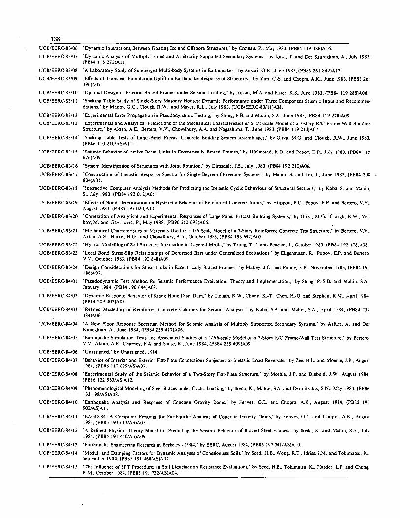
138
UCB/EERC-83/06 -Dynamic Interactions. Between Floating Ice and Offshore Structures: by Croteau, P., May 1983, (PB84 119 486jA 16.
UCB/EERC-83/07 -Dynamic Analysis of Multiply Tuned and Arbitrarily Supponed Secondary Systems: by Igusa, T. and Der Kiureghian, A., July 1983, (PB84 118 272jAII.
UCB/EERC-83/08 'A Laboratory Study of Submerged Multi-body Systems in Eanhquakes;- by Ansari, G.R., June 1983, (PB83 261 842jA17.
UCB/EERC-83/09 -Effects of Transient Foundation Uplift on Eanhquake Response of Structures: by Vim, e.-S. and Chopra, A.K., June 1983, (PB83 261 396jA07.
UCB/EERC-83/1O -Optimal Design of Friction-Braced Frames under Seismic Loading, - by Austin, M.A. and Pister, K.S., June 1983, (PB84 119 288jA06.
UCB/EERC-83/11 'Shaking Table Study of Single-Story Masonry Houses: Dynamic Performance under Three Component Seismic Input and Recommendations, - by Manos. G.C., Clough, R.W. and Mayes, RL., July 1983, (UCB/EERC-83/1IjA08.
UCB/EERC-83/12 -Experimental Error Propagation in Pseudodynamic Testing: by Shing, P.B. and Mahin, SA, June 1983, (PB84 119 270)A09.
UCB/EERC-83/13 -Experimental and Analytical Predictions of the Mechanical Characteristics of a lIS-scale Model of a 7-story RIC Frame-Wall Building Structure: by Aktan, A.E., Benero, V.V., Chowdhury, A.A. and Nagashima, T., June 1983, (PB84 119 213jA07.
UCB/EERC-83/14 -Shaking Table Tests of Large-Panel Precast Concrete Building System Assemblages: by Oliva, M.G. and Clough, R.W., June 1983, (PB86 110 210/ASjAII.·
UCB/EERC-83/IS -Seismic Behavior of Active Beam Links in Eccentrically Braced Frames," by Hjelmstad, K.D. and Popov, E.P., July 1983, (PB84 119 676jA09.
UCBlEERC-83/16 -System Identi~cation of Structures with Joint Rotation: by Dimsdale, J.S., July 1983, (PB84 192 21OjA06.
UCB/EERC-83/17 -Construction of Inelastic Response Spectra for Single-Degree-of-Freedom Systems: by Mahin, S. and Lin, J., June 1983, (PB84 208 834jAOS.
UCB/EERC-83/18 -Interactive Computer Analysis Methods for Predicting the Inelastic Cyclic Behaviour of Structural Sections: by Kaba, S. and Mahin. S., July 1983, (PB84 192 012jA06.
UCB/EERC-83/19 -Effects of Bond Deterioration on Hysteretic Behavior of Reinforced Concrete Joints: by Filippou, F.e., Popov, E.P. and Benero, V.V., August 1983. (PB84 192 020)A 10.
UCB/EERC-83/20 -Correlation of Analytical and Experimental Responses of Large-Panel Precast Building Systems," by Oliva, M.G., Gough, R.W .. Velkov, M. and Gavrilovic, P., May 1988, (PB90 262 6.92)A06.
UCB/EERC-83/21 'Mechanical Characteristics of Materials Used in a lIS Scale Model of a 7-Story Reinforced Concrete Test Structure: by Benero. v.v., Aktan, A.E.! Harris, H.G. and Chowdhury, A.A., October 1983. (PB84 193 697jAOS.
UCB/EERC-83/22 -Hybrid Modelling of Soil-Structure Interaction in Layered Media: by Tzong, T.-J. and Penzien, J., October 1983, (PB84 192 178jA08.
UCBlEERC-83/23 -Local Bond Stress-Slip Relationships of Deformed Bars under Generalized Excitations: by Eligehausen, R, Popov, E.P. and Benero, V.V., October 1983, (PB84 192 848jA09.
UCB/EERC-83/24 -Design Considerations for Shear Links in Eccentrically Braced Frames: by Malley, J.O. and Popov, E.P., November 1983, (PB84.192 I 86jA07.
UCB/EERC-84/01 -Pseudodynamic Test Method for Seismic Performance Evaluation: Theory and Implementation: by Shing, P.-S.B. and Mahin. SA, January 1984, (PB84 190 644)A08.
UCB/EERC-84/02 -Dynamic Response Behavior of Kiang Hong Dian Dam: by Clough, R.W., Chang, K.-T., Chen, H.-Q. and Stephen, R.M., April 1984, (PB84 209 402)A08.
UCB/EERC-84/03 . -Refined Modelling of Reinforced Concrete Columns for Seismic Analysis: by Kaba, S.A. and Mabin, SA, April 1984, (PB84 234 384)A06. .
UCBlEERC-84/04 -A New Floor Response Spectrum Method for Seismic Analysis of Multiply Supported Secondary Systems: by Asfura. A. and Der Kiureghian, A., June 1984, (PB84 239 417)A06.
UCB/EERC-84/0S 'Eanhquake Simulation Tests and Associated Studies of a IISth-scale Model of a 7-Story RIC Frame-Wall Test Structure: by Benero. V.V .• Aktan, A.E .• Charney, FA and Sause, R .• June 1984, (PB84 239 409)A09.
UCB/EERC-84/06 'Unassigned: by Unassigned, 1984.
UCBlEERC-84/07 -Behavior of Interior and Exterior Flat-Plate Connections Subjected to Inelastic Load Reversals, - by Zee, H.L. and Moehle, J.P., August 1984, (PB86 117 629/AS)A07.· .
UCB/EERC-84/08 -Experimental Study of the Seismic Behavior of a Two-Story Flat-Plate Structure: by Moehle, J.P. and Diebold. J.W., August 1984, (PB86 122 S53/AS)AI2. .
UCB/EERC-84/09 'Phenomenological Modeling of Steel Braces under Cyclic Loading, - by Ikeda, K.. Mahin, SA and Dermitzakis, S.N .. May 1984, (PB86 132 I 98/ASjA08.
UCB/EERC-84/10 -Earthquake Analysis and Response of Concrete Gravity Dams: by Fenves, G.L. and Chopra, A.K., August 1984, (PB85 193 902lASjAII.
UCB/EERC-84/11 -EAGD-84: A Computer Program for Eanhquake Analysis of Concrete Gravity Dams: by Fenves, G.L. and Chopra, A.K.. August 1984. (PB8S 193 613/ASjA05.
UCB/EERC-84/12 -A Refined Physical Theory Model for Predicting the Seismic Behavior of Braced Steel' Frames: by Ikeda, K. and Mahin, S.A., July 1984. (PB8S 191 4S0/ASjA09.
UCB/EERC-84/13 -Eanhquake Engineering Research at Berkeley - 1984," by EERC, August 1984, (PB8S 197 341/ASjA10.
UCB/EERC-84/14 -Moduli and Damping Factors for Dynamic Analyses of Cohesionless Soils: by Seed. H.B., Wong, R.T.. Idriss. I.M. and Tokimatsu. K .. September 1984. (PB85 191 468/AS)A04.
UCB/EERC-84/15 -The Influence of SPT Procedures in Soil Liquefaction Resistance Evaluations: by Seed, H.B., Tokimatsu, K., Harder. L.F. and Chung. R.M .. October 1984. (PB85 191 732/AS)A04.
139
UCB/EERC-84116 -Simplified Procedures for the Evaluation of Settlements in Sands Due to Earthquake Shaking, - by Tokimatsu, K. and Seed. H.B., October 1984, (PB85 197 8871ASjA03.
UCB/EERC-84/17 -Evaluation of Energy Absorption Characteristics of Highway Bridges Under Seismic Conditions - Volume I (PB90 262 627)A 16 and Volume II (Appendicesj (PB90 262 635jAIJ: by Imbsen, R.A. and Penzien, J., September 1986.
UCB/EERC-84/18 'Structure-Foundation Interactions under Dynamic Loads: by Liu, W.D. and Penzien, J., November 1984, (PB87 124 8891 AS)A II.
UCB/EERC-84/19 'Seismic Modelling of Deep Foundations: by Chen, C.-H. and Penzien, J., November 1984, (PB87 124 798/ASjA07.
UCB/EERC-84120 'Dynamic Response Behavior of Quan Shui Dam: by Clough, R.W., Chang, K.-T., Chen, H.-Q., Stephen, R.M., Ghanaat, Y. and Qi, J.-H., November 1984, (PB86 115177/ASjA07.
UCB/EERC-85101 -Simplified .Methods of Analysis for Earthquake Resistant Design of Buildings,' by Cruz, E.F. and Chopra, A.K., February 1985, (PB86 I I 22991AS)A I 2.
UCB/EERC-85102 'Estimation of Seismic Wave Coherency and Rupture Velocity using the SMART I Strong-Motion Array Recordings: by Abrahamson, N.A., March 1985, (PB86 214 343jA07.
UCBIEERC-85103 'Dynamic Properties of a Thirty Story Condominium Tower Building,' by Step ben, R.M., Wilson, E.L. and Stander, N., April 1985, (PB86 I I 8965/AS)A06.
UCBlEERC-85104 -Development of Substructuring Techniques for On-Line Computer Controlled Seismic Performance Testing,- by Dermitzakis, S. and Mahin, S., February 1985, (PB86 132941/ASjA08. .
UCBIEERC-85105 'A Simple Model for Reinforcing Bar Anchorages under Cyclic Excitations: by Filippou, F.C., March 1985, (PB86 112 9191 ASjA05.
UCBIEERC-85106 'Racking Behavior of Wood-framed Gypsum Panels under Dynamic Load, - by Oliva, M.G., June 1985, (PB90 262 643)A04.
UCB/EERC-85107 'Earthquake Analysis and Response of Concrete Arch Dams: by Fok, K.-L. and Chopra, A.K., June 1985, (PB86 I 39672JAS)AiO.
UCB/EERC-85108 'Effect of Inelastic Behavior on the Analysis and Design of Eartbquake Resistant Structures: by Lin, J.P. and Mahin, S.A., June 1985,
UC~/EERC-85109 'Earthquake Simulator Testing ofa Base,Isolated Bridge Deck,' by Kelly, J.M., Buckle, LG. and Tsai, H.-C., January 1986, (PB87 124 I 521AS)A06.
UCBIEERC-85110 'Simplified Analysis for Earthquake Resistant Design of Concrete Gravity Dams: by Fenves, G.l. and Chopra, A.K., June 1986, (PB87 124 160/ASjA08.
UCB/EERC-85111 'Dynamic Interaction Effects in Arch Dams: by Clough, R.W., Chang, K.-T., Chen, H.-Q. and Ghanaat, Y., October 1985, (PB86 I 35027/AS)A05.
UCBIEERC,85112 -Dynamic Response of Long Valley Dam in the Mammoth Lake Earthquake Series of May 25-27, 1980: by Lai, S. and Seed, H.B., November 1985. (PB86 I 423041ASjA05.
UCBIEERC-85/13 'A Methodology for Computer-Aided Design of Earthquake-Resistant Steel Structures, - by Austin, M.A., Pister, K.S. and Mahin, S.A., December 1985. (PB86 I 59480/AS)A10 .
UCBIEERC-85114 "Response of Tension-Leg Platforms to Vertical Seismic Ellcitations: by Liou, G.-S., Penzien, J. and Yeung, R.W., December 1985.
UCBIEERC-85115 'Cyclic Loading Tests of Masonry Single Piers: Volume 4 - Additional Tests with Height to Width Ratio of I: by Sveinsson, B .. McNiven, H.D. and Sucuoglu, H., December 1985, (PB87 I 65031/ASjA08.
UCBIEERC-85116 ' .... n Experimental Program for Studying the Dynamic Response of a Steel Frame with a Variety of [nfill Partitions, - by Yanev, B. and McNiven, H.D., December 1985, (PB90 262 676)A05.
UCBIEERC-86101 -A Study of Seismically Resistant Eccentrically Braced Steel Frame Systems; by Kasai, K. and Popov, E.P., January 1986, (PB87 124 1781 AS)A 14.
UCB/EERC-86/02 -Design Problems in Soil Liquefaction: by Seed, H.B., February 1986, (PB87 124 I 86/ASjA03.
UCB/EERC-86/03 'Implications of Recent Earthquakes and Research on Earthquake-Resistant Design and Construction of Buildings; by Bertero, V.V., March 1986, (PB87 124 I 94IAS)A05.
UCB/EERC,86/04 'The Use of Load Dependent Vectors for Dynamic and Earthquake Analyses: by Leger, P., Wilson, E.L. and Clough, R.W., March 1986, (PB87 124 202/AS)A12.
UCB/EERC-86/05 -Two Beam-To-Column Web Connections: by Tsai, K.-C. and Popov, E.P., April 1986, (PB87 124 301/AS)A04.
UCB/EERC-86/06 -Determination of Penetration Resistance for Coarse,Grained Soils using the Becker Hammer Drill: by Harder, l.F. and Seed. H.B., May 1986, (PB87 124 210IAS)A07.
UCB/EERC-86/07 'A Mathematical Model for Predicting the Nonlinear Response of Unreinforced Masonry Walls to In-Plane Earthquake Ellcitations: by Mengi, Y. and McNiven, H.D., May 1986, (PB87 124 780/AS)A06.
UCB/EERC-86/08 'The 19 September 1985 Mexico Earthquake: Building Behavior,' by Bertero, V.V., July 1986.
UCB/EERC-86/09 'EACD-3D: A Computer Program for Three,Dimensional Earthquake Analysis of Concrete Dams: by Fok, K.-L~ Hall, J.F. and Chopra. A.K., July 1986, (PBS7 124 228/AS)A08.
UCB/EERC-86/10 -Earthquake Simulation Tests and Associated Studies of a 0.3-Scale Model of a Six-Story Concentrically Braced Steel Structure: by Uang. C.-M. and Bertero, V.V., December 1986, (PB87 163 564/AS)AI7.
UCB/EERC-86111 'Mechanical Characteristics of Base Isolation Bearings for a Bridge Deck Model Test,' by Kelly, J.M., Buckle, I.G. and Koh, c.-G., November 1987. (PB90 262 668)A04.
UCBIEERC·86/12 'Effects of Axial load on Elastomeric Isolation Bearings: by Koh, C.-G. and Kelly, J.M., November 1987.
UCBIEERC,87101 -The FPS Eanhquake Resisting System: Ellperimental Report; by Zayas, V.A., low, S.S. and Mahin, S.A .. June 1987, (PB88 170 287)A06.
UCBIEERC,87/02 "Earthquake Simulator Tests and Associated Studies of a 0.3-Scale Model of a Six-Story Eccentrically Braced Steel Structure: by Whittaker. A .. Uang. C.,M. and Benero, V.V., July 1987, (PB88 166 7071ASjA18.
140
UCB/EERC·87/03 'A Displacement Control and Uplift Restraint Device for Base·lsolated Structures: by Kelly, J.M., Griffith, M.e. and Aiken, 1.0., April 1987, (PB88 169 933)A04.
UCB/EERC·87/04 'Earthquake Simulator Testing of a Combined Sliding Bearing and Rubber Bearing Isolation System: by Kelly, J.M. and Chalhoub, M.S., December 1990. -
UCB/EERC·87/05 ·Three·Dimensionallnelastic Analysis of Reinforced Concrete Frame·Wall Structures: by Moazzami, S. and Bertero. V.V., May 1987, (PB88 169 586/AS)A08.
UCB/EERC·87/06 'Experiments on Eccentrically Braced Frames with Composite Floors: by Rides, J. and Popov, E., June 1987. (PB88 173 067/AS)AI4.
UCB/EERC·87/07 'Oynamic Analysis of Seismically Resistant Eccentrically Braced Frames: by Rides, J. and Popov, E., June 1987, (PB88 173 0751 AS)A 16.
UCB/EERC·87/08 'Undrained CycliC Triaxial'Testing of Gravels-The Effect of Membrane Compliance: by Evans, M.D. and Seed, H.B., July 1987, (PB88 173 257)Al9.
UCB/EERC·87/09 'Hybrid Solution TeChniques for Generalized Pseudo-Dynamic Testing: by Thewalt, e. and Mahin, S.A., July 1987, (PB 88 179 007)A07.
UCB/EERC·87/10 'Ultimate Behavior of Butt Welded Splices in Heavy Rolled Steel Sections: by Bruneau, M., Mahin, S.A. and Popov, E.P., September 1987, (PB90 254 285)A07.
UCB/EERC·87/11 'Residual Strength of Sand from Dam Failures in the Chilean Earthquake of March 3, 1985: by De Alba, P., Seed, H.B., Retamal, E. and Seed, R.B., September 1987, (PBS8 174 321/AS)A03.
UCB/EERC·87/12 'Inelastic Seismic Response of Structures with Mass or Stiffness Eccentricities in Plan: by Bruneau, M. and Mahin, S.A., September 1987, (PB90 262 650/AS)AI4.
UCB/EERC·87/13 'CSTRUCT: An Interactive Computer Environment for the Design and Analysis of Earthquake Resistant Steel Structures: by Austin, M.A., Mahin, S.A. and Pister, K.S .. September 1987, (PB88 173 339/AS)A06.
UCBlEERC·87/14 'Experimental Study of Reinforced Concrete Columns -Subjected to Multi·Axial Loading: by Low, S.S. and Moehle; J.P., September 1987, (PB88 174 347/AS)A07.
UCB/EERC·87/15 'Relationships between Soil Conditions and Earthquake Ground Motions in Mexico City in the Earthquake of Sept. 19, 1985: by Seed, H.B., Romo, M.P., Sun, J., Jaime, A. and Lysmer, J., October 1987, (PB88 178 991)A06.
UCB/EERC·87/16 ··Experimental Study of Seismic Response orR. e. Setback Buildings: by Sbahrooz, B.M. and Moeble, J.P., October 1987, (PB88 176 359)AI6.
UCB/EERC·87/17 'The Effeet of Slabs on the Flexural Behavior of Beams: by Pantazopoulou. S.J. and Moehle, J.P., October 1987, (PB90 262 700)A07.
UCB/EERC·87/18 'Design Procedure for R·FBI Bearings: by Mostaghel, N. and Kelly, J.M .. November 1987, (PB90 262 718)A04.
UCB/EERC·87119 . Analytical Models for Predicting the Lateral Response of R C Shear Walls: Evaluation of their Reliability: by Vulcano. A. and Ber· tero, V. V .. November 1987, (PB88 178 983)A05.
UCB/EERC·87110 'Earthquake Response of Torsionally·Coupled Buildings: by Hejal, R.·and Cbopra, A.K., December 1987.
UCB/EERC·87/21 'Oynamic Reservoir Interaction with Monticello Darn: by Clough, R.W., Ghanaat, Y. and Qiu, X·F., December 1987, (PB88 179 023)A07. . .
UCBlEERC·87/22 'Strength Evaluation of Coarse·Grained Soils: by Siddiqi, F.H., Seed, R.B., Chan, e.K., Seed, H.B. and Pyke, R.M., December 1987, (PB88 179 031)A04.
UCBlEERC·88/01 'Seismic Behavior of Concentrically Braced Steel Frames: by Khatib, I., Mahin, S.A. and Pister, K.S., January 1988, (PB91 210 8981 AS)A II.
UCB/EERC·88/02 'Experimental Evaluation of Seismic Isolation of Medium·Rise Structures Subject to Uplift: by Griffith, M.e., Kelly, J.M., Coveney, V.A. and Koh, e.G., January 1988, (I"B91 217 950/AS)A09.
UCB/EERC·88/03 "Cyclic Behavior of Steel Double Angle Connections;' by Astaneh·Asl, A. and Nader, M.N., January 1988, (PB91 210 872)A05.
UCB/EERC·88/04 'Re-evaluation of the Slide in the Lower San Fernando Dam in the Earthquake of Feb. 9, 1971: by Seed, H.B., Seed, R.B., Harder, L.F. and Jong, H.·L., April 1988, (PB91 212 456/AS)A07.
UCB/EERC·88/05 'Experimental Evaluation of Seismic Isolation of a Nine·Story Braced Steel Frame Subject to Uplift: by Griffith, M.e., Kelly, J.M. and Aiken, 1.0., May 1988, (PB91 217 968/AS)A07.
UCB/EERC·88/06 ·DRAIN·2DX User Guide.,: by Allahabadi, R. and Powell, G.H., March 1988, (PB91 212 530)AI2.
UCB/EERC·88/07 'Theoretical and Experimental Studies of Cylindrical Water Tanks in Base·lsolated Structures: by Chalhoub, M.S. and Kelly, J.M., April 1988, (PB91 217 976/AS)A05.
UCB/EERC·88/08 'Analysis of Near·Source Waves: Separation of Wave Types Using Strong Motion Array Recording: by Darragh, R.B., June 1988, (PB91 212 621)A08,
UCB/EERC·88/09 . Alternatives to Standard Mode Superposition for Analysis of Non-Classically Damped Systems: by Kusainov, A.A. and Gough, R. W., June 1988, (PB91 217 992/AS)A04.
UCB/EERC·88/10 'The Landslide at the Pon of Nice on October 16, 1979: by Seed, H.B., Seed, R.B., Schlosser, F., Blondeau. F. and Juran. I., June 1988, (PB91 210 914)A05.
UCB/EERC·88/11 'Liquefaction Potential of Sand Deposits Under Low Levels of Excitation: by Caner, D.P. and Seed. H.B., August 1988. (PB91 210 880)AI5.
UCB/EERC·88/12 'Nonlinear Analysis of Reinforced Concrete Frames Under Cyclic Load Reversals: by Filippou. F.e. and Issa. A., September 1988, (PB91 112 589)A07.
UCB/EERC·88/13 'Implications of Recorded Earthquake Ground Motions on Seismic Design of Building Structures: by Uang. e.·M. and Benero. V.V .. November 1988. (PB91 212 548)A06.
141
UCB/EERC·88/14 . An Experimental Study of the Behavior of Dual Steel Systems: by Whittaker, A.S. , Uang, e.·M. and Bertero, V. V., September 1988, (PB91 212 712)AI6.
UCB/EERC·88/15 'Dynamic Moduli and Damping Ratios for Cohesive Soils: by Sun, ].I., Golesorkhi, R. and Seed, H.B., August 1988, (PB91 210 922)A04.
UCB/EERC·88/16 'Reinforced Concrete Flat Plates Under Lateral Load: An Experimeinal Study Including Biaxial Effects: by Pan, A. and Moehle, J.P., October 1988, (PB91 210 856)AI3.
UCB/EERC·88/17 'Earthquake Engineering Research at Berkeley. 1988: by EERC, November 1988, (PB91 210 864)AIO.
UCB/EERC·88/18 'Use of Energy as a Design Criterion in Earthquake·Resistant Design: by Uans. C.·M. and Bertero, V.V., November 1988, (PB91 210 906/AS)A04.
UCB/EERC·88/19 'Steel Beam·Column Joints in Seismic Moment Resisting Frames: by Tsai, K.·C. and Popov, E.P., November 1988, (PB91 217 .984/AS)A20.
UCB/EERC·88/20 'Base Isolation in Japan, 1988: by Kelly, J.M., December 1988, (PB91 212 449)A05.
UCB/EERC·89/01 'Behavior of Long Links in Eccentrically Braced Frames: by Engelhardt, M.D. and Popov, E.P., January 1989, (PB92 143 056)AI8.
UCB/EERC·89/02 'Earthquake Simulator Testing of Steel Plate Added Damping and Stiffness Elements: by Whittaker, A., Bertero, V.V., Alonso, J. and Thompson, C., January 1989, (PB91 229252JAS)AI0. .
UCB/EERC·89/03 'Implications of Site Effects in the Mexico City Earthquake of Sept. 19, 1985 for Earthquake-Resistant Design Criteria in the San Fran· . cisco Bay Area of Cali fomi a: by Seed, H.B. and Sun, J.I., March 1989, (PB91 229 369/AS)A07.
UCB/EERC·89/04 'Earthquake Analysis and Response of Intake·Outlet Towers,' by Goyal, A. and Chopra, A.K., July 1989, (PB91 229 286/AS)A 19.
UCB/EERC·89/0S 'The 1985 Chile Earthquake: An Evaluation of Structural Requirements for Bearing Wall Buildings: by Wallace, J.W. and Moehle, J.P., July 1989, (PB91 218 008/AS)AI3.
UCB/EERC·89/06 'Effects of Spatial Variation of Ground Motions on large Multiply·Supported Structures: by Hao, H., July 1989, (PB91 229 161/AS)A08.
UCB/EERC·89/07 ·EADAP· Enhanced Arch Dam Analysis Program: Users's Manual: by Ghanaat, Y. and Clough, R.W., August 1989, (PB91 212 522)A06.
UCB/EERC·89/08 'Seismic Performance of Steel Moment Frames Plastically Designed by Least Squares Stress Fields,' by Ohi, K. and Mahin, S.A., August 1989, (PB91 212 597jA05.
UCB/EERC·89/09 'Feasibility and Performance Studies on Improving the Earthquali:e Resistance of New and Existing Buildings Using the Friction Pendu· lum System: by Zayas, V., Low, S .. Mahin, SA and Bozzo, L., July 1989, (PB92 143 064)AI4.
UCB/EERC·89/10 'Measurement and Elimination of Membrane Compliance Effects in Undrained Triaxial Testing: by Nicholson, P.G., Seed, R,B. and Anwar, H., September 1989, (PB92 139 641/ASjA13.
UCB/EERC·89/11 'Static Tilt Behavior of Unanchored Cylindrical Tanks: by Lau, D.T. and Clough, R.W., September 1989, (PB92 143 049)AI0.
UCB/EERC·89/12 'ADAP·88: A Computer Program for Nonlinear Earthquake Analysis of Concrete Arch Dams: by Fenves; G.L., Mojtahedi, S. and Rei· mer, R.B., September 1989, (PB92 139 674/ASjA07.
UCB/EERC·89/13 'Mechanics of Low Shape Factor Elastomeric Seismic Isolation Bearings: by Aiken, I.D., Kelly, J.M. and Tajirian, F.F., November 1989, (PB92 139 7321AS)A09.
UCB/EERC·89/14 'Preliminary Report on the SeismolOgical and Engineering Aspects of the October 17, 1989 Santa Cruz (Loma Prieta) Earthquake,' by EERe. October 1989, (PB92 139 6821 AS)A04.
UCB/EERC·89/IS 'Experimental Studies of a.Singie Story Steel Structure Tested with Fixed, Semi· Rigid and Flexible Connections: by Nader, M.N. and Astaneh·Asl, A., August 1989, (PB91 229 211/AS)AI0.
UCB/EERC·89/16 "Collapse of the Cypress Street Viaduct as a Result of the Loma Prieta Earthquake: by Nims, D.K., Miranda, E., Aiken, I.D., Whit· taker, A.S. and Bertero, V.V., November 1989, (PB91 217 935/ASjA05.
UCB/EERC·90/01 'Mechanics of High·Shape Factor Elastomeric Seismic Isolation Bearings: by Kelly, J.M., Aiken, I.D. and Tajirian, F.E, March 1990.
UCB/EERC,90102 • Javid's Paradox: The Influence of Preform on the Modes of Vibrating Beams: hy Kelly, J.M., Sackman, J.L. and Javid~ A., May 1990,
UCB/EERC·90/03 'Earthquake Simulator Testing and Analytical Studies of Two Energy·Absorbing Systems for Multistory Structures,' by Aiken, J.D. and Kelly, J.M .. October 1990, (PB92 192 988jAI3.
UCB/EERC·90/04 'Damage to the San Francisco-Oakland Bay Bridge During the October 17, 1989 Earthquake: by Astaneh·Asl, A., June 1990.
UCB/EERC·90/0S 'Preliminary Report on the Principal Geotechnical Aspects of the OctOber 17, 1989 Loma Prieta Earthquake: by Seed. R.B., Dicken· son, S.E., Riemer. M.F., Bray, J.D., Sitar, N., Mitchell, J.K., ldriss, J.M., Kayen, R.E., Kropp, A., Harder, L.F., Jr. and Power, M.S .• April 1990. (PB 192 970jA08.
UCBIEERC·90106 'Models of Critical Regions in Reinforced Concrete Frames Under Seismic Excitations: by Zulfiqar, N. and Filippou, F.e., May 1990.
UCBIEERC·90/07 'A Unified Earthquake·Resistant Design Method for Steel Frames Using ARMA Models: by Takewaki, I., Conte, J.P., Mahin, S.A. and Pister, K.S., June 1990.
UCB/EERC·90/08 'Soil Conditions and Earthquake Hazard Mitigation in the Marina District of San Francisco: by Mitchell, J.K., Masood, T., Kayen, R.E. and Seed, R.B .. May 1990. (PB 193 2671ASjA04.
UCB/EERC·90/09 'Influence of the Earthquake Ground MOlion Process and Structural Properties on Response Characteristics of Simple Structures: by Conte. J.P., Pister. K.S. and Mahin. SA. July 1990. (PB92 143 064)AIS.
UCB/EERC·90110 'Experimental Testing of the Resilient·Friction Base Isolation System: by Clark, P.W. and Kelly, J.M .. July 1990. (PB92 143 072)A08.
UCB/EERC·90111 'Seismic Hazard Analysis: Improved Models. Uncertainties and SenSitivities: by Araya. R. and Der Kiureghian. A .. March 1988.
UCBIEERC·90112 'Effects of Torsion on Ihe Linear and Nonlinear Seismic Response of Siructures," by Sedarat, H. and Bertero. V.V .. September 1989.
142
UCB/EERC-90/13 -The Effects of Tectonic Movements on Stresses and Defonnations in Earth Embankments: by Bray, J. D., Seed, R. B. and Seed, H. B., September 1989.
UCB/EERC-90/14 -Inelastic Seismic Response of One-Story, Asymmetric-Plan Systems: by Goel, R.K. and Chopra, A.K., October 1990.
UCBIEERC-90115 -Dynamic Crack Propagation: A Model for Near-Field Ground Motion.: by Seyyedian, H. and Kelly, J.M., 1990.
UCBIEERC-90/16 -Sensitivity of Long-Period Response Spectra to System Initial Conditions: by Blasquez, R., Ventura, e. and Kelly, J.M., 1990.
UCB/EERC-90/17
UCB/EERC-90/18
UCBIEERC-90/19
UCB/EERC-90120
UCB/EERC-90/21
UCB/EERC-91101
UCB/EERC-91102
UCB/EERC-91/03
-Behavior of Peak Values and Spectral Ordinates of Near-Source Strong Ground-Motion over a Dense Array, - by Niazi, M., June 1990.
-Material Characterization of Elastomers used in Earthquake Base ISOlation: by Papoulia, K.D. and Kelly, J.M., 1990.
-Cyclic Behavior of Steel Top-and-Bottom Plate Moment Connections: by Harriott, J.D. and Astaneh-Asl, A., August 1990, (PB91 229 260/AS)A05.
-Seismic Response Evaluation of an Instrumented Six Story Steel Building: by Shen, J.-H. and Astaneh-Asl, A., December 1990, (PB91 229294IAS)A04.
-Observations and Implications of Tests on the Cypress Street Viaduct Test Structure: by Bolio, M., Mahin, S.A., Moehle, J.P., Stephen, R.M. and Qi, X., December 1990.
-Experimental Evaluation of Nitinol for Energy Dissipation in Structures: by Nims, D.K., Sasaki, K.K. and Kelly, J.M., 1991.
-Displacement Design Approach for Reinforced Concrete Structures Subjected to Earthquakes: by Qi, X. and Moehle, J.P., January 1991, (PB93 114 569/AS)A09.
-A Long-Period Isolation System Using Low-Modulus High-Damping Isolators for Nudear Facilities at Soft-Soil Sites: by Kelly, J.M., March 1991,(PB93 114 577IAS)AIO.
UCB/EERC-91/04 -Dynamic and Failure Characteristics of Bridgestone Isolation Bearings: by Kelly, J.M., April 1991, (PB93 114 528)A05.
UCBIEERC-91105 -Base Sliding Response of Concrete Gravity Dams to Earthquakes: by Chopra, A.K. and Zhang, L., May 1991, (PB93' 114 544/AS)A05.
UCB/EERC-91106 "Computation of Spatially Varying Ground Motion and Foundation-Rock Impedance Matrices for Seismic Analysis of Arch Dams: by Zhang, L. and Chopra, A.K., May 1991, (PB93 114 825)A07.
UCBIEERC-91/07 -Estimation of Seismic Source Processes Using Strong Motion Array Data: by Chiou, S.-1., July 1991, (PB93 114 551/AS)A08.
UCBIEERC-91/08 -A Response Spectrum Method for Multiple-Support Seismic Excitations: by Der Kiureghian, A. and Neuenhofer, A_, August 1991. (PB93 114 536)A04.
UCB/EERC-91109 -A Preliminary Study on Energy Dissipating Cladding-to-Frame Connection: by Cohen, J.M. and Powell, G.H., September 1991, (PB93 114510)A05.
UCBIEERC-91110 -Evaluation of Seismic Performance of a Ten-Story RC Building During the Whittier Narrows Eanhquake: by Miranda, E. and Bertero, V.V., October 1991, + (PB93 114 783)A06.
UCBIEERC-91111 -Seismic Performance of an Instrumented Six Story Steel Building: by Anderson, I.e. and Bertero, V.V., November 1991.
UCB/EERC-91/12 -Perfonnance of Improved Ground During the Loma Prieta Eanhquake: by MitChell, J.K. and Wentz, Jr., F.J., October 1991, (PB9} 114791)A06.
UCBIEERC-91113 -Shaking Table - Structure Interaction: by Rinawi, A.M. and Clough, R.w., October 1991, (PB93 114 917)A13.
UCB/EERC-91/14 -Cydic Response of RC Beam-Column Knee Joints: Test and Retrofit: by Mazzoni, S., Moehle, J.P. and Thewalt, e.R., October 1991, (PB93 120 277)A03.
UCB/EERC-91/15 -Design Guidelines for Ductility and Drift Limits: Review of State-of-the-Practice and State-of-the-Art in Ductility and Drift-Based Eanhquake-Resistant Design of Buildings: by Bertero, V.V., Anderson, J.e., Krawink.ler, H., Miranda, E. and The CUREe and The Kajima Research Teams, July 1991, (PB93 120 269)A08.
UCBIEERC-91/16 -Evaluation of the Seismic Performance of a Thirty-Story RC Building: by Anderson, J.e., Miranda, E., Bertero, V.V. and The Kajima Project Research Team, July 1991, (PB93 114 841)AI2.
UCB/EERC-9 1 I 17 -A Fiber Beam-Column Element for Seismic Response Analysis of Reinforced Concrete Structures, - by Taucer, F., Spacone, E. and Filippou, F.e., December 1991. .
/
~0272-101 /-------------------------~\
:REPO::RT=~=AG=~M=EN=TA=nO=N~IL-N_;-~~/ ........ E_:--G_~-9_-1-0_1-7_-_-_-_-:_-:_-r-I'--2..~-_-_-_-_-_-_+'T":""":!..---:.l"~I"_"I_II_I_I~!~~11~~~~ll~_"I1I~1 ~r 4.. Tlts •• nd Subtltl. 5. R~ o.te
December 1991 "A fiber beam-column element for seismic response analysis of reinforced concrete structures"
7_~.) L P.,'o" .. lnC OrpnluOoft R.ot. No. Fabio Taucer, Enrico Spacone, and Filip C. Filippou UCB/EERC~9l/ 17
,. P9rlotm1nc Orpnlution Name and Add,....
Earthquake Engineering Research Center ,University of California, Berkeley '1301 SO. 46th Street
11. eona--t(C) or Gnlrc(G') No.
(e)
Richmond, Calif. 94804 (G') RTA-59M848 ECE-8657525
National Science Foundation 1800 G ,S tree t, N. W . Washington, D.C. 20550
California Dept. of Transportation 1801 3th Street Sacramento, CA 95816 14.
16.. Abstnct (Umlt: 200 ........cal - '"
~ ~"-c~::'~-"~, "~-='~~-~This study proposes a reliable and computationally efficient beam-column finite element model for the analysis of reinforced concrete members under cyclic loading conditions that induce biaxial bending and axial force. The element is discretized into longitudinal steel and concrete fibers such that the section force-deformation relation is derived by integration of the stress-strain relation of the fibers. At present, the nonlinear behavlor of the element derlves entlrely from the nonlinear stress-seraln relation of the steel and concrete fibers(- =-=,-.-, ,=«
The proposed beam-column element is based on the assumption that deformati'ons are small and that plane seceions remain plane during the loading history. The formulation of the element is based on the mixed method: the description of the force distribution within the element by interpolation functions that satisfy equilibrium is the starting point of the formulation. Based on the concepts of the mixed method, it is shown that the selection of flexibility dependent shape functions for the deformation field of the element results in considerable simplification of the final equations.
A special flexibility based state determination algorithm is proposed for the computation of the stiffness matrix and resisting forces of the beam-column element.
A new scheme for the application of element loads in flexibility based beam finite elements is also presented ln the report. The procedure lS a natural extension of the element state determination algorithm and is based on the use of the exact internal force distribution under the applied element loads. The corresponding fixed end forces at the element ends are determined during iterations of the element state determination.
17. Doc:u.-..t An..1,...r. a. o..:riptwol
Release Unlimited
_ ANS1-ZJ9.181
1 g,. Security Cs-a (11Ita ReportJ
unclassified 2D. Sec:urtty Clau (1111 ...... )
unclassified
21. No. 01 Pacd 155,
OPT1OHAL. F'ORloi rn (4-m (Fo ...... rIy NTls-J51 OeP.~ 01 Comm....:a

::-; ,
.-