pacific earthquake engineering research center...richard o. zerbe anthony falit-baiamonte university...
TRANSCRIPT

Richard O. ZerbeAnthony Falit-Baiamonte
University of Washington
The Use of Benefit-Cost Analysis for Evaluation ofPerformance-Based Earthquake Engineering Decisions
Pacific Earthquake EngineeringResearch Center
PEER 2002/06SEPTEMBER 2001
A report on research conducted undergrant no. CMS-9812531 from the National Science Foundation:
U.S.-Japan Cooperative Research in Urban Earthquake Disaster Mitigation

The Use of Benefit-Cost Analysis for Evaluation of Performance-Based Earthquake Engineering
Decisions
Richard O. Zerbe Evans School of Public Affairs
University of Washington
and
Anthony Falit-Baiamonte Department of Geography University of Washington
A report on research conducted under grant no. CMS-98121531 from the National Science Foundation:
U.S.-Japan Cooperative Research in Urban Earthquake Disaster Mitigation
PEER Report 2002/06 Pacific Earthquake Engineering Research Center
College of Engineering University of California, Berkeley
September 2001

iii
ABSTRACT
This report provides an overview of benefit-cost analysis (BCA); an application of benefit-cost
analysis to the performance-based earthquake engineering (PBEE) framework; consideration of
critical issues in using benefit-cost analysis for PBEE; and a discussion of issues, criticism, and
limitations of benefit-cost analysis. Our objective is to provide an understanding of the
economic dimensions of PEER’s framework equation. A focus on economic evaluation will
broaden the framework so that facility damage in earthquakes can be related to functionality,
business interruption and revenue loss, and to repair costs. Such an analysis needs to consider
issues such as the time value of money, uncertainty, and the perspectives of different
stakeholders.
The application of BCA to PBEE has produced a number of important findings. First, an
example is developed that illustrates the way in which performance criteria can be
operationalized in an economic context. Next, a number of benefit categories are identified (cost
of emergency response and loss of long-term revenue) that have not been previously considered
in studies of seismic mitigation decision making. Additionally, several critical issues are
examined, most notably multiple stakeholders and uncertainty, that need to be considered when
carrying out a benefit-cost analysis in a performance-based engineering context.
Throughout the report, particular attention is paid to issues of concern to PEER
researchers and the seismic-mitigation community, most notably, the differences between BCA
and life cycle cost analysis (LCCA). These differences are extensively discussed and illustrated.
Finally the ways in which the value of human life can be economically evaluated are examined.

iv
ACKNOWLEDGMENTS
This work was supported in part by the Pacific Earthquake Engineering Research Center through
the Earthquake Engineering Research Centers Program of the National Science Foundation
under Award number EEC-9701568.
We would like to thank Stephanie Chang, Peter May, and Mary Comerio for their useful
comments.

v
PREFACE
The Pacific Earthquake Engineering Research Center (PEER) is an Earthquake Engineering
Research Center administered under the National Science Foundation Engineering Research
Center program. The mission of PEER is to develop and disseminate technology for design and
construction of buildings and infrastructure to meet the diverse seismic performance needs of
owners and society. Current approaches to seismic design are indirect in their use of information
on earthquakes, system response to earthquakes, and owner and societal needs. These current
approaches produce buildings and infrastructure whose performance is highly variable, and may
not meet the needs of owners and society. The PEER program aims to develop a performance-
based earthquake engineering approach that can be used to produce systems of predictable and
appropriate seismic performance.
To accomplish its mission, PEER has organized a program built around research,
education, and technology transfer. The research program merges engineering seismology,
structural and geotechnical engineering, and socio-economic considerations in coordinated
studies to develop fundamental information and enabling technologies that are evaluated and
refined using test beds. Primary emphases of the research program at this time are on older
existing concrete buildings, bridges, and highways. The education program promotes
engineering awareness in the general public and trains undergraduate and graduate students to
conduct research and to implement research findings developed in the PEER program. The
technology transfer program involves practicing earthquake professionals, government agencies,
and specific industry sectors in PEER programs to promote implementation of appropriate new
technologies. Technology transfer is enhanced through a formal outreach program.
PEER has commissioned a series of synthesis reports with a goal being to summarize
information relevant to PEER’s research program. These reports are intended to reflect progress
in many, but not all, of the research areas in which PEER is active. Furthermore, the synthesis
reports are geared toward informed earthquake engineering professionals who are well versed in
the fundamentals of earthquake engineering, but are not necessarily experts in the various fields
covered by the reports. Indeed, one of the primary goals of the reports is to foster cross-
discipline collaboration by summarizing the relevant knowledge in the various fields. A related
purpose of the reports is to identify where knowledge is well developed and, conversely, where

vi
significant gaps exist. This information will help form the basis to establish future research
initiatives within PEER.

vii
CONTENTS
ABSTRACT.................................................................................................................................. iii
ACKNOWLEDGMENTS ........................................................................................................... iv
PREFACE.......................................................................................................................................v
TABLE OF CONTENTS ........................................................................................................... vii
LIST OF FIGURES ..................................................................................................................... xi
LIST OF TABLES ..................................................................................................................... xiii
1 OVERVIEW OF BENEFIT-COST ANALYSIS................................................................1
1.1 Introduction.....................................................................................................................1
1.2 Theoretical Foundations..................................................................................................3
1.2.1 Benefit-Cost Analysis as Economic Evaluation ...............................................4
1.2.2 Efficiency Criteria ............................................................................................5
1.3 Current Use of BCA in the United States .......................................................................7
1.3.1 Federal Government .........................................................................................7
1.3.2 State Governments............................................................................................8
1.3.3 Municipal Governments ...................................................................................8
1.3.4 Seismic Decision Making .................................................................................9
1.4 Understanding the Role of Benefit-Cost Analysis ..........................................................9
1.5 Steps of Benefit-Cost Analysis .....................................................................................10
1.5.1 Clarifying the Perspective...............................................................................10
1.5.2 Set Out the Assumptions ................................................................................10
1.5.3 Determine Benefits and Costs, Relevant Data, and Cash Flows ....................10
1.5.4 Present Value and Discount Rate ...................................................................14
1.5.5 Treatment of Inflation.....................................................................................14
1.5.6 Choosing a Criterion.......................................................................................15
1.5.7 Applying the Criterion....................................................................................16
1.5.8 Dealing with Uncertainty................................................................................16
1.5.9 Decision ..........................................................................................................17
1.5.10 Feedback .........................................................................................................17
1.5.11 General Equilibrium .......................................................................................17
viii
1.6 Summary of BCA Framework ......................................................................................18
1.7 Performing BCA: A Simplified Earthquake Example ..................................................18
1.7.1 Make Clear for Whom Analysis Is Performed ...............................................19
1.7.2 Set Out Assumptions ......................................................................................19
1.7.3 Determine Relevant Data and Set Out Cash Flows ........................................20
1.8 Life-Cycle Cost Analysis ..............................................................................................21
1.9 Contributions of BCA ...................................................................................................23
1.10 Gains from Further Application of BCA ......................................................................24
1.11 Limitations of Benefit-Cost Analysis............................................................................25
2 APPLICATION OF BENEFIT-COST ANALYSIS TO PERFORMANCE- BASED EARTHQUAKE ENGINEERING FRAMEWORK .........................................27
2.1 Economic Evaluation of Seismically Vulnerable Systems ...........................................28
2.2 Economic Evaluation of Performance Criteria .............................................................28
2.3 Earthquake Mitigation Costs and Benefits for Ports.....................................................30
3 CRITICAL ISSUES IN USING BENEFIT-COST ANALYSIS FOR PBEE ................33
3.1 Scale/Multiple Stakeholder Analysis ............................................................................33
3.2 Uncertainty ....................................................................................................................33
4 ISSUES, CRITICISM, AND LIMITATIONS OF BENEFIT-COST ANALYSIS........35
4.1 Foundational Issues for BCA........................................................................................35
4.2 Criticism Explained.......................................................................................................35
4.2.1 Technical Limitations .....................................................................................35
4.2.2 Moral Criticism...............................................................................................37
4.3 Foundational Criticism Resolved..................................................................................37
4.3.1 KHZ Criterion as an Answer to Moral and Technical Criticism....................37
4.3.2 KHZ Characteristics .......................................................................................38
4.3.3 Missing Values ...............................................................................................39
4.4 Process Issues and Criticism .........................................................................................43
4.5 Process Criticism Addressed: Suggestions for Improving Process..............................44
4.6 Issues of Practice...........................................................................................................45

ix
4.6.1 Discount Rate..................................................................................................45
4.7 Limitations of Benefit-Cost Analysis............................................................................47
4.8 Conclusions...................................................................................................................47
APPENDIX A DISCOUNT RATE ........................................................................................50
APPENDIX B BENEFIT-COST PROTOCOL FOR EVALUATING PERFORMANCE-BASED EARTHQUAKE ENGINEERING DECISIONS AT MARINE PORTS.............................................................57
REFERENCES ..........................................................................................................................79

xi
LIST OF FIGURES
2.1 Earthquake Mitigation Costs and Benefits for Ports ...................................................... 31
B.2.1 Earthquake Mitigation Costs and Benefits for Ports ...................................................... 64
B.2.2 Probabilistic Valuation Model ........................................................................................ 74

xiii
LIST OF TABLES
1.1 Benefits and Costs in Relation to Gains and Losses.........................................................11
1.2 Quality of Life Ratings .....................................................................................................13
1.3 Advantages and Disadvantages of Evaluation Criteria ....................................................15
1.4 Cash Flows and Present Values........................................................................................20
1.5 Net Present Value .............................................................................................................21
1.6 Summary of Benefit-Cost Analysis ..................................................................................22
1.7 Life-Cycle Costs ...............................................................................................................22
2.1 Hypothetical Seismic Hazards Curve ...............................................................................29
4.1 The Discount Rate Problem Resolved..............................................................................42
A.1 SRTP and Shadow Price of Capital ..................................................................................53
A.2 Variable Ranges................................................................................................................54
A.3 Ferat Trials........................................................................................................................54
A.4 Frequency Distribution .....................................................................................................55
B.2.1 Hypothetical Seismic Hazards Curve ...............................................................................62
B.2.2 Hypothetical Seismic Construction Cost for Each Mitigation Option .............................65
B.2.3 Hypothetical Outputs of Component Vulnerability Analysis...........................................67
B.2.4 Hypothetical Cost of Response for Each Mitigation Option ............................................68
B.2.5 Short-Term Loss of Revenue Associated with Each Mitigation Option ..........................71
B.2.6 Long-Term Loss of Revenue Associated with Each Mitigation Option ..........................72
B.2.7 Calculation of Expected Value of Benefits of Each Mitigation Option ...........................75
B.2.8 Calculation of Present Value for the M1 Mitigation Option ............................................76
B.2.9 Distribution of NPVs for Each Mitigation Option ...........................................................77

1
1 Overview of Benefit-Cost Analysis
1.1 INTRODUCTION
This report considers the use of benefit-cost analysis (BCA) for the evaluation of performance-
based earthquake engineering (PBEE) decisions. Our objective is to provide an understanding of
the economic dimensions of PEER’s framework equation, which relates measures of ground
motion to measures of damage and system performance. For the most part, research that utilizes
this or similar frameworks tends to focus on physical damage and the resultant financial and life-
safety losses (Cornell and Krawinkler 2000). A more explicit economic analysis will broaden
the framework so that facility damage in earthquakes can be related to functionality, business
interruption and revenue loss, and to repair costs. Such an analysis needs to consider issues such
as the time value of money, uncertainty, and the perspective of different stakeholders.
The report provides an overview of benefit-cost analysis; an application of benefit-cost
analysis to the performance-based earthquake engineering framework; consideration of critical
issues in using benefit-cost analysis for PBEE, and a discussion of issues, criticism, and
limitations of benefit-cost analysis. This report should prove useful to a wide variety of PEER
researchers and industry and government partners, including those who are not experts. In
addition to providing a theoretical and methodological primer on the use of BCA, we explicitly
consider how BCA can be adapted to the performance-based earthquake engineering framework.
The application of benefit-cost analysis to a hypothetical PBEE scenario provides a clear
illustration of how to implement this type of analysis. It also demonstrates the types of
parameters (inputs and outputs) required in order to incorporate a benefit-cost component into an
integrated computer application.
The application of BCA to PBEE has produced a number of important findings. First, an
example is developed that illustrates the way in which performance criteria can be
operationalized in an economic context. A number of benefit categories are identified (cost of
2
emergency response and loss of long-term revenue) that have not been previously considered in
studies of seismic mitigation decision making. Additionally, several critical issues are examined,
most notably multiple stakeholders and uncertainty, that are essential to carrying out a benefit-
cost analysis in a performance-based engineering context. Throughout the report, areas are
suggested for further development and coordination with other PEER researchers.
Chapter 1 of the report provides an overview of benefit-cost analysis. We begin by
offering a brief review of the theoretical underpinnings of BCA that focuses on BCA as a method
to economically evaluate seismic mitigation decisions. We then provide a more practical view
of BCA, with a step-by-step procedure for applying the BCA framework and by explaining key
concepts (time value of money, present value, discount rate, treatment of inflation, evaluation
criteria, and uncertainty). A simplified example is used to illustrate the steps of the BCA
framework. Additionally, we discuss the current use of BCA in governmental agencies and the
seismic mitigation community. Throughout this introductory section, particular attention is paid
to issues of concern to PEER researchers and the seismic mitigation community, most notably to
the differences between BCA and life-cycle cost analysis (LCCA), a commonly used method of
evaluation for seismic mitigation decisions. The ways in which the value of human life can be
economically evaluated are also discussed and illustrated.
Chapter 2 demonstrates how BCA can be adapted to accommodate the performance-
based earthquake engineering framework. For the most part this section provides an overview of
a protocol developed by the PEER Zerbe and Chang project. This protocol, complete with a
hypothetical example, is attached as an appendix to the report. Although the specifics of the
protocol and hypothetical example focus on marine ports, both the conceptual framework and
methodological approach can be generalized to other types of seismically vulnerable systems.
Currently, the protocol is being developed into a booklet for distribution to various port agencies.
The application of BCA to PBEE provides a clear illustration of how to implement this type of
analysis. More important, it has produced a number of significant findings. The analysis that is
undertaken in Appendix B utilizes performance standards provided by the Port of Oakland. We
operationalize the criteria in order to specify the benefits and costs of seismic mitigation options
in performance-based terms. While we do not claim to have developed a definitive methodology
for operationalizing and specifying performance criteria, our effort can serve as the basis of
discussion among PEER research and industry and government partners. Our research with the
Port of Oakland, supplemented by reviews of seismic decision making, benefit-cost analysis, and

3
ports literature, also identified a number of benefit categories not previously considered. We
define benefits as savings on costs that would not have occurred without mitigation.
Traditionally, seismic BCA considers only benefits associated with savings on facility repair
costs. We demonstrate that the cost of measures taken in order to respond to a seismic
emergency are not insignificant and should be considered as part of the analysis. Additionally,
loss of revenue needs to be considered with respect to both the structure of the economic market
in which the facility operates and the time value of money. Consequently, we distinguish
between short-term revenue loss (that lost during repair to a facility) and long-term revenue loss
(permanent revenue loss due to loss of customers). In terms of BCA, these categories are
“discounted” differently in order to correctly account for the time value of money.
Our analysis of the application of BCA to PBEE indicates that several critical issues need
to be considered further. These are discussed in Chapter 3. At this time, many of these issues
are being addressed by research in progress. While traditional BCA considers only the
perspective of the “primary” stakeholder, a variety of groups are differentially affected by the
benefits and costs associated with performance-based earthquake engineering decisions. The
Zerbe-Chang PEER project is developing a new framework that will theoretically and
methodologically incorporate the perspective of multiple stakeholders — the owner of the
structure, the user(s)/tenant(s) of the structure, the local economy, the regional economy, and
“society.” This type of analysis will provide the opportunity for collaboration with a number of
PEER researchers and partners. A second critical issue that needs to be addressed is uncertainty.
Wilkie's PEER project (Caltech) is considering the probabilistic aspects of uncertainty in terms
of performance-based mitigation options, while the Zerbe-Chang project is addressing the proper
use of other techniques for considering uncertainty.
Chapter 4, the final substantive section of the report, considers criticism and limitations
of BCA. Both technical and ethical issues are outlined, discussed, and in some cases resolved.
Additionally, several suggestions are made for improving the BCA process.
1.2 THEORETICAL FOUNDATIONS
Benefit-cost analysis (BCA) is a subset of policy analysis. It involves an accounting framework
in which benefits and costs associated with decisions are set out for purposes of information and
4
discussion.1 The details of the framework are of course important and while there is significant
agreement about them, there is room for improvement. BCA attempts to provide decision makers
with preferred policy alternatives, including the alternative of doing nothing.
Life-cycle cost analysis (LCCA), which is commonly used in the evaluation of seismic
mitigation decisions, may be properly viewed as a subcategory of benefit-cost analysis. It is
simply another way of expressing the results of a benefit-cost analysis. LCCA involves the
determination of the costs of all options. When these options are compared the results are
similar to the results of benefit-cost analysis.
Another subcategory of BCA is cost-effectiveness analysis. Cost-effectiveness analysis
presumes that a policy decision about the goal or objective to be reached has already been made
and that the only matter to resolve is the best way of meeting the specific policy chosen. For
example, consider a policy discussion about whether to dam a river to produce electricity or to
leave it alone to provide recreation benefits. A BCA would consider all of the alternatives.
However, if a decision already had been made in favor of the dam, then a cost-effectiveness
analysis would determine the most economically efficient dam to build (i.e., the one providing
the greatest net benefits). Other important examples of cost-effectiveness analyses are air and
water pollution standards. Normally, the question that arises with these standards is how to
achieve them at the least cost.
1.2.1 Benefit-Cost Analysis as Economic Evaluation
BCA provides a means of economically evaluating a project that involves seismic mitigation
decisions. Economic evaluation is performed in order to determine the most economically
efficient mitigation option, the option that maximizes the difference between benefits and costs.
In terms of seismic mitigation decisions, this simply involves the maximization of net revenues.
The economic theory perspective is that such analysis should be done from a national
perspective that comprises the values of all affected. This view has a certain naiveté when
compared with practice, where the cost of considering all affected may limit the extent of values
and people considered. Drawing upon current issues, difficult questions arise: Should a policy
affecting the costs of abortions count the costs to fetuses? Should the public education benefits
1 Benefit-Cost Analysis and Cost-Benefit analysis are used identically. We prefer the former term as closer to its
theoretical roots in economics and as implying perhaps a less mechanistic version.

5
to the children of illegal aliens be included in an analysis of the educational policies? Should the
benefits criminals receive from crime be counted in considering policies affecting criminal
behavior? Should the existence value of environmental amenities be counted? Should harm to
animals receive economic weight? These types of questions are called “issues of economic
standing” (Whittington and Macrae 1986; Zerbe 2002). Although some types of BCAs are
usually done from the perspective of a single entity, such as a public utility district or the owner
of a building, without any pretense of a national perspective, the benefits and costs associated
with performance-based earthquake engineering decisions will differentially affect a wide variety
of parties, or stakeholders. Traditionally, BCA considers only the perspective of the “primary”
stakeholder. The new framework under development in the Zerbe-Chang PEER project will in
theory and methodology incorporate the perspective of multiple stakeholders — the owner(s) of
the site, the user(s)/tenant(s) of the site, the local economy, the regional economy, and “society”
(see Chapter 3.1).
1.2.2 Efficiency Criteria
BCA is based on a normative standard that economists call the Kaldor-Hicks (KH) criteria, or the
potential Pareto criteria. The latter is derived from the notion of Pareto efficiency but is
fundamentally different in that only a potential Pareto improvement is required. According to
Pareto efficiency a policy is justified when someone gains and no one loses. According to the
KH criteria it is sufficient if the losers can be compensated, even if they are not, so that in
principle the Pareto requirement can be met while ignoring the costs of actually making income
transfers.2 A policy is then said to be KH efficient when the winner from the project could
potentially compensate the project loser.3 The KH efficiency criteria have existed as an important
concept in both economics and law for more than 60 years. A computerized search of law
reviews and legal journals finds nearly 2,000 citations to Kaldor-Hicks or its synonyms.4 Thus
2 Pareto efficiency is more or less useless for practical policy work as examples of policies that met the criterion are
not generally to be found. 3 For a more precise definition see Zerbe 2001. The Kaldor and Hicks are actually slightly different criteria. 4 I found 425 references to “Kaldor-Hicks” directly; 92 more are found under the rubric “potential Pareto,” and
1416 cites are to some form of “wealth maximization.” The numbers reported here were generated by three Westlaw searches on October 29, 1997, all of which were conducted using the “Journals of Law Reviews” database.
6
not only has BCA contributed to project evaluation but also to legal reasoning both in the United
States and in Europe.
The criteria arose out of discussions in the late 1930s among prominent British
economists concerning whether or not repeal of the Corn Laws was good.5 Lionel Robbins
(1938, p. 640) had asserted that economists could not claim that policies that had losers were
desirable, as would be created by repeal of the Corn Laws, as this claim was necessarily based on
interpersonal comparisons.
Kaldor (1939, pp. 549–50) acknowledged Robbins’s point about the inability to make
interpersonal utility comparisons, but suggested its irrelevance. He suggested that where a
policy led to an increase in aggregate real income:
the economist’s case for the policy is quite unaffected by the question of the comparability of individual satisfaction, since in all such cases it is possible to make everybody better off than before, or at any rate to make some people better off without making anybody worse off.
Kaldor goes on to note (1939, p. 550) that whether such compensation should take place “is a
political question on which the economist, qua economist, could hardly pronounce.” Kaldor then
proposed a potential compensation test and Hicks followed with a similar test. 6
These two tests are known as the Kaldor-Hicks compensation tests,7 or, alternatively, as
the potential compensation — or potential Pareto — tests.8 They represent what economists and
5 These are Robbins, Hicks, and Kaldor all writing in the Economic Journal.
6 Kaldor’s (1939) suggestion was later formalized as the proposition that:
“state a is preferable to another state if, in state a, it is hypothetically possible to undertake costless (lump-sum) redistribution and achieve an allocation that is superior to the other state according to the Pareto criterion” ( Boadway and Bruce 1984, p. 96). Hicks (1939) suggested a parallel test, which is formally stated as: “state A is preferable to another state if, in the other state, it is not possible, hypothetically, to carry out lump-sum
redistribution so that everyone could be made as well off as in state A.” See Boadway and Bruce (1984, p. 97). 7 Chipman (1987, p. 524) suggests that the compensation principle may be traced back to Dupuit in 1844, and, later,
to Marshall (1890). Marshall used the concept of consumer surplus to compare losses of consumers to gains to the government. Hotelling (1938) anticipated the KH test by suggesting that a new public investment is justified, given its benefits, if its costs could — in theory — be distributed in order to make everyone better off. Anticipating issues of distribution, Hotelling (1938) noted that where extreme hardship resulted from a policy, actual compensation was needed.
8 The term “Kaldor-Hicks” was used at least as early as 1951, by Arrow (1951, p. 928), and in 1952, by Mishan (1952, p. 312).

7
lawyers mean by “economic efficiency.”9 Posner (1985, pp. 88–89; 1986, pp. 12–13; 1987, p.
16) as indicated that a term of his creation, “wealth maximization,” is identical to KH. Although
he has not always been consistent, this definition is assumed here.10
1.3 CURRENT USE OF BCA IN THE UNITED STATES
1.3.1 Federal Government
BCA rose to prominence at the federal level with the analysis of water projects during the 1940s
and became more widespread in use under Presidents Carter and especially Reagan and Bush.
President Clinton reaffirmed a commitment to BCA.11 For example, as a response to Executive
Order No. 12291 and subsequent orders, federal executive agencies are required to use BCA as
part of the regulatory process. Under these executive orders, the Office of Management and the
Budget (OMB) has created a set of guidelines that should be the starting point for any
governmental unit considering adopting benefit-cost guidelines. 12 Recent attempts to pass
benefit-cost legislation show the continuing appeal of a methodology that holds out the promise
of introducing greater rationality into the regulatory process.13 In terms of earthquake mitigation,
FEMA has issued a set of BCA guidelines. Our final draft will summarize and comment upon
these guidelines.
9 The other concept, of course, is that of Pareto optimality, but this is a concept ill suited to discussion of economic
changes and is, therefore, of limited practical application. 10 “Wealth maximization” appears to have an imprecise meaning. Posner (1987) sometimes uses wealth
maximization to mean KH, but at other times seems to use it to mean an increase in GDP or the maximization of monetary wealth. In this regard, Posner uses it to support his tastes in favor of a work ethic and the importance of production as compared with consumption. This is, however, a different meaning from KH. The fact that economic efficiency is not the same as national income was shown by Harberger (1971, p. 785). Economic efficiency is the opposite of common but narrow concepts, such as workplace efficiency in which people are to be managed as machines (Kanigel 1997).
11 See Executive Order No. 12,866, 3 C.F.R. 638 (1994) reprinted in 5 U.S.C. s 601 (1994) ; Executive Order No. 12,498, 3 C.F.R. 323 (1986) reprinted in 5 U.S.C. s 601 (1988); Executive Order 12291, 3 C.F.R. 127 (1982) reprinted in 5 U.S.C s 601 (1988) (revoked in 1993). For a delineation of the criticism of these orders and a discussion, see Pildes and. Sunstein 1995.
12Circular A-94.
131995 US HB. 1022 (SN). The House bill was called “The Risk Assessment and Cost Benefit Act of 1995.” According to the statute, the purpose of the legislation is to “reform regulatory agencies and focus national economic resources...through scientifically objective and unbiased risk assessments and through the consideration of costs and benefits in major rules.” The floor debate suggests that an implication of this requirement is that a criterion would be adopted so that only those regulations with a net positive outcome would be promulgated. This is an example of attempting to use the result of a BCA as the decision itself.

8
1.3.2 State Governments
The extent to which BCA is used among state governments is not wholly known. Eight states
have statutes requiring the application of some cost analysis, economic impact analysis, or BCA.
These are Arizona, California, Colorado, Florida, Illinois, Oregon, Virginia, Washington, and
Wisconsin. The State of Washington, for example, requires nine enumerated agencies to14
Determine that the probable benefits of the rule are greater than its probable costs, taking into account both the qualitative and quantitative benefits and costs and the specific directives of the statute being implemented.15
The rulemaking criteria section of the act requires that the mandated agencies also consider
alternatives to the rule, including the consequences of not adopting the rule. The agency is
required to adopt the “least burdensome” rule that gives positive net benefits.
1.3.3 Municipal Governments
Dively and Zerbe (1991) conducted a survey of the practices of municipal governments to make
investment and policy decisions. This survey used telephone and written questionnaires for a
randomly selected sample of 72 American cities with populations over 100,000 in the fall of
1990 and the spring of 1991. The authors found that almost 60% of the cities surveyed did not
use discount rates; in fact, in some of these cities, officials did not understand the meaning of the
term. The use of the discount rate shows an appreciation for the time value of money (see section
1.5.4 and Appendix A), this concept is critical to BCA.
By examining the effects of city age, population, growth in population, presence of
municipally owned utilities, bond rating, presence of independently elected officials, and
geographical location, Dively and Zerbe (1991) attempted to explain why some cities but not
others use discount rates. The only variable that showed statistical significance in prediction was
“independently-elected financial officials”; cities with such officials are more likely to use
discount rates. Officials in older cities also appear more likely to use discount rates although this
variable did not quite reach statistical significance.
14
Chapter 403, Washington Law, 1995 (Engrossed Substitute House Bill 1010, partially vetoed) effective July 23, 1995.
15This requirement applies only to those rules that are not procedural or interpretive.
9
The importance of independently elected financial officials was found to be consistent
with answers provided by city officials after informal questioning about why program budgeting
and discount rates were not used. The most common answer was that the use of these techniques
imposed a constraint on decisions that were based primarily on political considerations. That
result is also consistent with the finding of Rauch (1995) that the professionalism of the state
bureaucracy during the Progressive Era had a positive effect on the share of municipal
expenditure allocated to investment in infrastructure (probably greater efficiency in allocation).
These results suggest that increasing the number of cities with independently elected financial
officials would increase the use of discount rates and associated capital budgeting techniques,
with a probable increase in economic efficiency.16
1.3.4 Seismic Decision Making
As was noted above, FEMA has issued a set of BCA guidelines. Additionally, many entities
concerned with seismic mitigation decisions, especially public agencies, often use some type of
BCA in the decision-making process. However, this analysis is often performed in a way that
does not consider critical issues in a structured and systematic manner. The following sections
will provide a framework that outlines, considers, and illustrates a number of issues that we
consider to be crucial to the benefit-cost analysis.
1.4 UNDERSTANDING THE ROLE OF BENEFIT-COST ANALYSIS
BCA is an accounting framework that provides an understanding of the ways in which the
benefits and costs associated with seismic mitigation will affect the revenue of a particular entity
over time. However, the particular way in which BCA is performed can affect the context in
which decisions will be discussed and made. While BCA does not directly determine decisions,
it sets the framework for the decision-making process. Politics also plays a role in this process.
In addition, benefit-cost analysis, as every rational decision process, has limitations because it
necessarily deals with uncertainty, measurement problems, and limited funds for evaluation.
Given these considerations, it should be recognized that within a policy context, BCA provides
information for decision makers and not just the decision itself.
16
Our hypothesis is that the presence of such officials leads to a higher standard of review. Interestingly, the use of

10
1.5 STEPS OF BENEFIT-COST ANALYSIS
While BCA is often performed in an ad hoc manner, it is most useful when the process follows a
set of well-defined steps. Adherence to these steps ensures that all assumptions, calculations,
and criteria are clearly acknowledged.
1.5.1 Clarifying the Perspective
The results of a benefit-cost analysis will depend on the perspective from which it is performed.
Although in its most economically supportable use the analysis is done from a national
perspective, more often than not the perspective used is that of the agency performing the
analysis or the perspective of the particular branch of government. Given the sensitivity of
results to the perspective, this should be made clear at the outset.
1.5.2 Set Out Assumptions
The precepts of good policy analysis require that assumptions be set out early. This is especially
the case with BCA, where one purpose is to contribute information to the discussion. Among the
assumptions that need to be addressed are (1) the perspective from which the analysis is done
(step 1.5.1 above); (2) what parties, values, and interests are included and which are excluded;
(3) the discount rate used; (4) how robust the results are with respect to other assumptions; and
(5) uncertainty.
1.5.3 Determine Benefits and Costs, Relevant Data, and Cash Flows
Benefits and costs have traditionally been based on the willingness to pay (WTP) and the
willingness to accept (WTA). These concepts have been related in turn to measures of welfare
changes that use either final (after-project) prices or initial (before-project) prices and are
referred to as “compensating variation” and “equivalent variation measures.” These complex
relationships will not be explored here. Table 1.1 relates benefits-costs to gains and losses and to
WTP and WTA measures. In the tradition of pure benefit-cost analysis, the WTP and WTA of all
parties affected are to be counted with legal rights to determine whether or not the WTP (for
non-owners) or WTA (for owners) is more appropriate. As previously stated, because benefit-
discount rates by cities with independently elected officials is double the rate for a sample of cities as a whole.

11
cost analyses are often done from particular perspectives, in terms of performance-based
earthquake engineering, gains and losses will likely depend on whose perspective is being
addressed. From the perspective of a public utility district, for example, efficiency might be
defined in terms of changes in net revenues.
Table 1.1 Benefits and Costs in Relation to Gains and Losses
Benefit: Gain
WTP: amount one is willing to pay for
positive change—limited by income (a
positive amount)
Example: the amount an entity would pay to
reduce the probability of earthquake damage
Cost: Loss
WTA: minimum amount one is willing to
accept as compensation for a negative
change—could be infinite (a negative
amount)
Example: the amount an entity spends to
reduce the probability of earthquake damage.
According to Table 1.1, gains should be measured by the willingness to pay for them
(WTP) and losses by the willingness to accept payment (WTA) for them.17 Where goods are
valued only for their ability to create revenues, the WTP and WTA measures will be the same.
Such goods have been called “commercial goods” (Zerbe 2001). For commercial goods the
value of the good is essentially the present value of the commercial cash flows. For example, the
value of a truck to an entity concerned with seismic mitigation will be the same whether or not
one uses WTP or WTA. For other goods, however, ownership or rights matters. As valued by
environmentalists, the value of a pristine park that might be damaged by an earthquake would be
quite different if measured by the WTP instead of the WTA. If an environmental group were
given the right to be compensated for loss of a park, for example, the relevant measure would be
the group's WTA, which in principle could be infinite. If the group had no such right, the correct
measure would be the WTP, which would be limited by what the group could pay.
17 A loss restored is a benefit, but in psychological terms is not a gain but a restoration to some status quo. A gain
forgone can be a cost, but again it is not a loss from a psychological reference point.
12
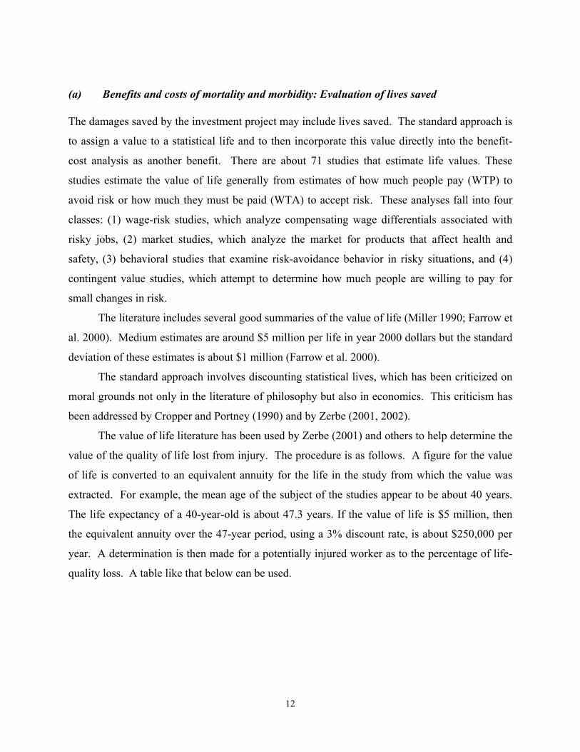
(a) Benefits and costs of mortality and morbidity: Evaluation of lives saved
The damages saved by the investment project may include lives saved. The standard approach is
to assign a value to a statistical life and to then incorporate this value directly into the benefit-
cost analysis as another benefit. There are about 71 studies that estimate life values. These
studies estimate the value of life generally from estimates of how much people pay (WTP) to
avoid risk or how much they must be paid (WTA) to accept risk. These analyses fall into four
classes: (1) wage-risk studies, which analyze compensating wage differentials associated with
risky jobs, (2) market studies, which analyze the market for products that affect health and
safety, (3) behavioral studies that examine risk-avoidance behavior in risky situations, and (4)
contingent value studies, which attempt to determine how much people are willing to pay for
small changes in risk.
The literature includes several good summaries of the value of life (Miller 1990; Farrow et
al. 2000). Medium estimates are around $5 million per life in year 2000 dollars but the standard
deviation of these estimates is about $1 million (Farrow et al. 2000).
The standard approach involves discounting statistical lives, which has been criticized on
moral grounds not only in the literature of philosophy but also in economics. This criticism has
been addressed by Cropper and Portney (1990) and by Zerbe (2001, 2002).
The value of life literature has been used by Zerbe (2001) and others to help determine the
value of the quality of life lost from injury. The procedure is as follows. A figure for the value
of life is converted to an equivalent annuity for the life in the study from which the value was
extracted. For example, the mean age of the subject of the studies appear to be about 40 years.
The life expectancy of a 40-year-old is about 47.3 years. If the value of life is $5 million, then
the equivalent annuity over the 47-year period, using a 3% discount rate, is about $250,000 per
year. A determination is then made for a potentially injured worker as to the percentage of life-
quality loss. A table like that below can be used.

13
Table 1.2 Quality of Life Ratings
Distress Rating⇒
Disability Rating⇓
A. No distress
B. Mild C. Moderate D. Severe
1. No disability 0.995 0.990 0.967
2. Slight social
disability
1.00 0.986 0.973 0.932
3. Severe social
disability and/or
slight physical
impairment
0.980 0.972 0.956 0.912
4. Physical ability
severely limited (e.g.
light housework only)
0.964 0.956 0.942 0.870
5. Unable to take paid
employment or
education, largely
housebound
0.946 0.935 0.900 0.700
6. Confined to chair
or wheelchair but
able to move around
in house with
assistance
0.875 0.845 0.680 0.00
7. Confined to bed 0.677 0.564 0.000 -1.468
8. Unconscious -1.028 n/a n/a n/a Source: Kind et al., 1982. Notes: healthy = 1; dead = 0.00; n/a = not applicable; the negative figures indicate a life worse than death.
The numbers in Table 1.2 are the percentage of normal quality of life (1.00). Thus, a
rating of 0.70 suggests that a person unable to take paid employment who is largely housebound
and who suffers from severe distress has about 70% of the quality of life of a normal person.
Thus with a potential injury lasting for 5 years and during which time one-half of the quality of
life is lost, then the calculation would show a loss of 0.5 (the quality of life lost) times the value
of life of $250,000 per year.

14
1.5.4 Present Value and Discount Rate
Many of the evaluation criteria for BCA require that future benefits and costs be reduced to a
present value so that comparisons between different projects or alternatives will be consistent.
The present value of a given cash flow is just the sum of money that if invested today at some
relevant interest rate will yield that cash flow. For example, $100 invested today at a 10% will
yield $10 each year forever. Thus, the present value of a cash flow of $10 per year forever,
discounted at 10%, is just $100. (To find the present value of a cash flow that continues forever,
called a perpetuity, the amount of the cash flow is divided by the interest rate. In this case we
have $10/(0.10) = $100. When the interest rate is used in this fashion we call it the discount rate.
The larger the interest rate or discount rate, the smaller will be the present value of
positive cash flows. For example, the present value of $100 to be received in 20 years is $81.95
at a 1% discount rate but is $14.86 at a 10% rate. The choice of discount rate can have a major
impact on the present value of a cash flow.
While an extensive technical literature discusses the appropriate choice of discount rate
(See Appendix A),18 there is nevertheless a growing expectation that the appropriate discount rate
will reflect the cost of capital for a term similar to the life of the project for the government
organization considering a project. This rate is approximately the rate on government bonds that
mature at about the time the project is to be completed. Thus, in the above example, 7% is used
as the nominal (not adjusted for inflation) discount rate.
1.5.5 Treatment of Inflation
The cash flows (constant dollars) listed in Table 1.2 do not account for inflation, but cash flows
adjusted for inflation are also used in a BCA. Whichever type of discount rate is used must be
consistent with the type of dollars represented by the cash flows. A discount rate reflecting
constant or inflation-adjusted dollars is called a real discount rate; one that reflects current or
nominal dollars is called the market or nominal discount rate.
Since the current example uses constant dollars, we would use a discount rate of 7% (i.e.,
10% – 3%) as the discount rate for the cash flows listed in Table 1.2; that is, the difference
18
A comprehensive discussion of discounting can also be found in Lind (1982).

15
between 10% and 3% gives the inflation-adjusted discount rate of 7%. Using the current dollar
amounts, 7% would be the discount rate. The results would be the same.19
1.5.6 Choosing a Criterion
After setting out the cash flows, benefits and costs need to be compared. Several different
evaluative criteria in widespread use (Zerbe and Dively, 1994) include the net present value
(NPV), benefits-costs (B/C) ratios, the internal rate of return (IRR), payback period, and the
wealth maximizing rate (WMR). Each has certain advantages and disadvantages, shown below
in Table 1.3, and discussed in greater length by Zerbe and Dively (1994).
Table 1.3 Advantages and Disadvantages of Evaluation Criteria*
NPV B/C PAYBACK IRR WMR
always gives right answer for
a single project
X X 0 0 X
gives right answer when
comparing projects
X 0 0 0 0
widely used X
(econ)
X
(business)
X
(elect.
industry)
X 0
(newly
developed)
answer is easily understood 0 X X X X
easily adjusted to give
right answer for single or
multiple projects
NA X 0 0 X
can be adjusted to give right
answer
NA NA 0 X NA
*NA= not applicable; X= yes and 0= no
All of these criteria can be used efficiently except that the payback period is inappropriate
where time periods are very different or cash flows uneven. The NPV can be used generally
without adjustments or special attention. Note that the benefit-cost ratio may not rank projects
correctly when comparing them.
19
They will be approximately the same where subtraction is used to find the real rate. They will be exactly the same where the more accurate approach of division, as shown in the previous footnote, is used to find the real discount rate.

16
1.5.7 Applying the Criterion
Once a criterion is chosen, the benefits and costs are compared by calculations.
1.5.8 Dealing with Uncertainty
Uncertainty addresses the ways in which the costs and benefits would differ if the conditions or
circumstances of analysis were altered. In general, uncertainty analysis requires realistic
estimates of benefit and cost categories as well as variance around these estimates. While
traditional approaches to uncertainty analysis are important components of any BCA, PEER
research is currently exploring uncertainty analysis in the context of PBEE. More specifically,
Wilkie's project is considering the probabilistic aspects of uncertainty in terms of mitigation
options, and the Zerbe-Chang project is addressing the relationship between risk and uncertainty
(see Chapter 3.2).
(a) Methods of approach
While several standard techniques consider uncertainty, such as sensitivity analysis, stochastic
dominance, and risk-adjusted interest rates, there are no clear guidelines for when to use a
particular technique. This raises a particularly egregious issue in considering risk-adjusted
interest rates. The risk-adjusted interest rates technique is commonly used by businesses for
evaluating projects, but is less often used by governments. This issue will be addressed further
in connection with a protocol we developed that also provides guidelines for the proper use of
other techniques for considering uncertainty.
(b) Sensitivity analysis
Uncertainty is of particular concern given the probabilistic nature of natural disasters. A useful
and straightforward way to handle uncertainty is to perform a sensitivity analysis. Such an
analysis gives some insight into how the project would perform were conditions or
circumstances different from those anticipated, for example, the effect if the capital costs were
higher by 20% and the probability of a seismic event were lower by 10%. The result of this
would be to reduce the benefits and to increase the costs.

17
1.5.9 Decision
The BCA should be regarded as information relevant to the decision process, and not just the
decision (Zerbe and Dively 1994; Zerbe 1998b; Hahn 1986). Even though the financial analysis
may suggest that the project is a good one, there may be factors not captured by this analysis. For
example, an entity considering seismic mitigation may be concerned with environmental
objections to the proposed project.
Sometimes benefits or costs can not be quantified. In these cases the analyst should point
to this out and stress that these uncertainties should be part of the decision-making process.
1.5.10 Feedback
Once a project is complete it is uncommon but quite helpful to reevaluate the benefit-cost
predictions in terms of what actually happened so that the analyst can improve the BCA
technique in the future.
1.5.11 General Equilibrium
Most benefit-cost analyses are “partial equilibrium,” that is, they examine the effects on supply
and demand in one or few markets. “General equilibrium” analyses model the interactions
between markets and account for the simultaneous determination of prices and incomes
throughout an economy. For example, a 50-cent-per-gallon gas tax nationwide will have an
economic impact far beyond the gasoline market. First, it will affect the demand for related
goods such as automobiles. Second, it will affect the demand for productive resources such as
automobile workers, which might in turn affect the supply of workers for related industries.
Finally, how the government spends tax money will in turn affect various markets. A BCA that
considers the effects of an earthquake can account for the effects on a region or the nation. Each
might be either partial or general equilibrium. Within a region there will be many goods; an
analysis that accounts for them just within the region would be a “limited general equilibrium
analysis.” In examining the effects on the nation, just a single good might be considered and not
account for effects from markets that would otherwise be affected. In this case the analysis might
bear more resemblance to partial equilibrium.
It is possible to account for general equilibrium welfare effects by examining only those
markets directly affected and those indirectly affected that have distortions. A distortion is an

18
effect that drives a wedge between supply and demand. The primary examples are taxes and
monopoly power, so indirectly affected markets with these distortions need to be examined.
1.6 SUMMARY BCA FRAMEWORK
1. The role of BCA is to provide information and structure to the decision process, not just
to provide the decision.
2. When analyzing even simple projects, a number of questions must be answered. These
include the choice of interest or discount rate, treatment of inflation and uncertainty, and
the choice of evaluation criteria.
3. The following steps are required as a minimum as part of BCA:
• Make clear the client for whom the analysis is being performed.
• Set out the assumptions of the analysis.
• Set out relevant data and the cash flows (benefits and costs).
• Choose the appropriate discount rate appropriately adjusted for inflation.
• Choose an appropriate evaluation criterion, e.g., NPV.
• Apply the chosen criterion, e.g., reduce to NPV.
• Allow for uncertainty: Perform a sensitivity analysis.
• Make a decision.
• Provide feedback: Perform a post-perspective analysis.
1.7 PERFORMING BCA: A SIMPLIFIED EARTHQUAKE EXAMPLE
A simple use of BCA might the case of a building owner who is considering a seismic retrofit.
The owner wishes to determine whether the investment would be wise from a financial
standpoint.
Even with this seemingly straightforward problem, a number of important issues are
present, including the treatment of uncertainty, the determination of relevant cash flows, the
appropriate discount rate, the data assumptions, and the choice of evaluation criteria.
Suppose that the improvement costs $1 million. One way to pose the question of the
improvement is to ask, “Will the investment of $1 million yield more for the building owner than
an alternative investment?” Another is, “Will the savings the owner expects from buying the
19
improvement represent a return greater than what it could otherwise earn, for example, by
putting the money in the bank?”20 To answer these questions, consider the basic steps of a BCA.
1.7.1 Make Clear for Whom the Analysis Is Performed (Who is the Client/Stakeholder?)
In this case the client is the owner of the building in question.
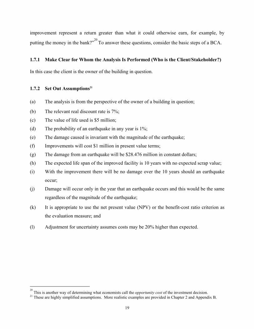
1.7.2 Set Out Assumptions21
(a) The analysis is from the perspective of the owner of a building in question;
(b) The relevant real discount rate is 7%;
(c) The value of life used is $5 million;
(d) The probability of an earthquake in any year is 1%;
(e) The damage caused is invariant with the magnitude of the earthquake;
(f) Improvements will cost $1 million in present value terms;
(g) The damage from an earthquake will be $28.476 million in constant dollars;
(h) The expected life span of the improved facility is 10 years with no expected scrap value;
(i) With the improvement there will be no damage over the 10 years should an earthquake
occur;
(j) Damage will occur only in the year that an earthquake occurs and this would be the same
regardless of the magnitude of the earthquake;
(k) It is appropriate to use the net present value (NPV) or the benefit-cost ratio criterion as
the evaluation measure; and
(l) Adjustment for uncertainty assumes costs may be 20% higher than expected.
20
This is another way of determining what economists call the opportunity cost of the investment decision. 21 These are highly simplified assumptions. More realistic examples are provided in Chapter 2 and Appendix B.

20
1.7.3 Determine Relevant Data and Set Out Cash Flows
By purchasing the improvement, the owner will not have to incur expenditures to repair damage
from an earthquake. Should an earthquake occur, the damage is expected to be $28.476 million
in the year of the event and zero thereafter. This amount is expected to increase with inflation, as
measured by the Gross Domestic Product Implicit Price Deflator. The real discount estimate is
based on an estimate of 10% for the cost of capital and a foreseeable expected inflation of 3%
annually; this is accounted for by the 7% real discount rate (10%–3%).
The second part of this step is to determine the annual cash flows associated with each
alternative. These are shown in Table 4 (below). We make the conventional assumption that the
cash flows are received at the end of each time period (here years) except for the initial
expenditure. (If one has information to the contrary such as, for example, that benefits will be
received in the middle of the period, this can be accounted for in setting out the cash flows.)
Table 1.4 Cash Flows and Present Values (Adjusted for Inflation)
YEAR COST
(in millions)
DAMAGE
(in millions)
PROBABILITY OF
DAMAGE
SAVINGS IN
DAMAGE
(millions)
PRESENT
VALUE OF
SAVINGS
(millions)
0 -1.0000
1 28.4755 1% 0.2848 0.2661
2 28.4755 1% 0.2848 0.2487
3 28.4755 1% 0.2848 0.2324
4 28.4755 1% 0.2848 0.2172
5 28.4755 1% 0.2848 0.2030
6 28.4755 1% 0.2848 0.1897
7 28.4755 1% 0.2848 0.1773
8 28.4755 1% 0.28476 0.1657
9 28.4755 1% 0.28476 0.1548
10 28.4755 1% 0.28476 0.1447
Table 1.5 summarizes the results of Table 1.4 into two summary criteria, the NPV and the
benefit-cost ratio.

21
Table 1.5 Net Present Value PRESENT VALUE
OF BENEFITS
(Sum from Table 1.4
(millions))
PRESENT VALUE
OF COSTS
(millions)
BENEFITS
MINUS
COSTS
(NPV)
BENEFIT-
COST RATIO
(B/C)
2.000 1.000 1.000 2.00
One source of confusion is the distinction between constant and current dollars. Benefits
and costs are listed in constant dollars, that is adjusted for the effects of inflation. Current
dollars, are not adjusted for inflation. The benefits from avoiding earthquake damage are listed
in constant dollars. The actual amounts will increase with inflation. By listing the constant
dollar amount and adjusting the discount rate for inflation, the results are the same as if inflation
were included and a 10% rather than a 7% discount rate were used.
1.8 LIFE-CYCLE COST ANALYSIS
Life-cycle cost analysis (LCCA) has received much attention in recent years within the
earthquake engineering community and as a potential framework for use by PEER in evaluating
increased performance of earthquake engineering measures. Illustrations of the potential
applicability of this decision framework for seismic risk reduction include discussion of
applicability to port facilities (e.g., Taylor and Werner 1995; Werner et al. 1997) bridges, (e.g.,
Chang and Shinozuka 1996), water systems (e.g., Chang et al. 1998), and buildings.
More generally, the U.S. Department of Transportation has encouraged states to employ
life-cycle cost analysis for evaluating major transportation projects in keeping with federal
highway legislation and executive orders (see U.S. Federal Highway Administration 1996).
Life-cycle cost analysis has also been heavily promoted by the federal government as a tool for
evaluating investments in energy-efficient devices.
The above problem is considered as a simple example of the relation between BCA and
LCCA. For a particular structural design, life-cycle costs consist of the present value of expected
costs from construction of the facility to the end of the structural life-span (Chang and
Shinozuka, 1996). Life-cycle costs include construction, maintenance and, when done from a
broader perspective, user costs. User costs for a transportation project, for example, might
include increased travel time, increased accident costs, and increased vehicle-operating costs.

22
Items that in one case might appear as costs, such as increased travel time, might in another
appear as benefits, such as decreased travel time.
LCCA is simply another way of expressing the results of a benefit-cost analysis and
generally involves the determination of costs of all options. When these options are compared,
the result is the same as that of a benefit-cost analysis. Consider the following example of a
performance standard to reduce earthquake damage. Table 1.6 gives a summary BCA analysis
of the Port of Seattle performance standard project; Table 1.7 uses life-cycle costs.
Table 1.6 Summary of Benefit-Cost Analysis Net Present Value (NPV) +$1. 00
Table 1.7 Life-Cycle Costs
Performance
Standard A
Do Nothing
Option
Value of
Performance
Standard A over
Do Nothing
Costs of Construction -$1.00 $0 -$1.00
Costs of Earthquake -$0.00 -$2.00 +$2.00
Total Life Cycle Costs -$1.00 -$200. +$1.00
Life-cycle cost approach is another way of presenting the results of a benefit-cost
analysis. No information is lost in LCCA; one need simply keep in mind that benefits are the
costs of options forgone.
One problem that can arise with LCCA that is more easily avoided with benefit-cost
analysis is that economic measures of benefits are generally different from those for costs.
Benefits are measured by WTP and costs by WTA. In some cases these measures can diverge
significantly. Thus, in benefit-cost analysis issues arise about what count as benefits or costs.
Life-cycle cost analysis can obscure this distinction.
Where benefits and costs are considered for commercial goods—goods for which there is
no divergence between the WTP and the WTA, such as occurs when gains and losses are borne
by corporations, this issue is not likely to arise. It is most likely to be an issue when gains and
losses involve important non-market goods such as an environmental good.
23
One advantage of LCCA over benefit-cost analysis lies in its emphasis of comparison of
alternatives. LCCA may make it more likely that alternative courses of action are actually
considered. In addition, many analysts favor LCCA because it more clearly sets out the future
maintenance cost implications of an investment decision.
The life-cycle and benefit-cost decision frameworks are appealing for a number of
reasons. First, they draw attention to long-run costs. This makes it possible to consider trade-
offs such as higher up-front costs and reduced downstream repair costs or costs of business
disruption. Second, they provide a single metric — dollars, appropriately discounted, for
evaluating choice outcomes. This overcomes the difficulties of comparing outcomes with
respect to discrete, incommensurate objectives (e.g., lives lost, business interrupted, injuries).
But there is still the problem of how to monetarize lives lost, etc. This also provides a continuous
scale for making relative comparisons of value of different choices. Third, the frameworks are
flexible enough to allow for incorporation of different time horizons, discounting factors, and
changing components for benefit or cost streams.
1.9 CONTRIBUTIONS OF BCA
Over the years, the quality of BCA has improved: the government uses more appropriate interest
or discount rates; values such as environmental values that once were not considered are now
included; assumptions are made clearer. These improvements have arisen from the structure of
BCA. A principal advantage of BCA is that it provides a framework for rational discussion and
allows for a critique of information relevant for the decision-making process. Similarly, the use
of efficiency analysis in legal reasoning has contributed to an understanding of law and allowed
a critique of efficiency reasoning in the law (Zerbe 1998b). A careful student of the use of BCA
(Lave 1996, p. 130) notes that “...I praise it for forcing analysts to think systematically about
social issues, collect data, and do analyses to clarify the implication of decisions.” Farrow (2000,
p. 2) notes that the use of BCA as part of executive office review is associated with rejecting
some regulations that would have been economically inefficient.
Nevertheless, the extent to which BCAs have improved the policy process remains
somewhat unclear. What is clear is that improvement is possible.

24
1.10 GAINS FROM FURTHER APPLICATION OF BCA
Consensus among prominent commentators suggests that substantial gains exist from further
application of BCA at every level of government. BCA has been used to stop a number of
unappealing projects. Criticism by economists of project analyses done by the U.S. Army Corps
of Engineers, the Bureau of Reclamation, and the Tennessee Valley Authority, for example, has
prevented the funding of inefficient projects but has also improved the quality of the benefit-cost
analyses done by these organizations.
Work by Graham (1995) and Tengs et al. (1996) suggests that even in the United States a
reallocation of resources to more cost-effective programs could save 60,000 lives per year at no
increased cost to taxpayers or to industry.22 The use of BCA, just beginning at the state level, is
used by less than one half of the municipal governments with populations over 100,000. Thus
one may conclude that there is substantial room for expanding the use of BCA in the U.S (and
even more so in Europe).23
Hahn (1996, p. 239) finds that about one half of the regulatory rules in the U.S. would not
pass a benefit-cost test, even using numbers provided by government agencies, which he finds
overstate benefits. According to Hahn (p. 231), EPA regulations are relatively poor in terms of
their cost-effectiveness as measured by the cost per life saved.
He finds further that “. . .agencies could improve regulations by implementing a strategic
planning process that uses net economic benefits as a criterion in deciding how to allocate
agency resources.” Hahn (p. 243) concludes that “performed well and taken seriously cost-
benefit analysis can and should aid in the selection and design of more economically efficient
policies.”
22
Graham 1995, 62. 23
This is not to suggest that all regulations should be based strictly on benefit-cost tests. It makes little sense to subject policies whose primary goals are non-economic, e.g., the improvement of human rights or the rights of nature, to strict economic analysis. Of course, in a secondary sense, any such policies should be implemented as efficiently as possible.
25
1.11 LIMITATIONS OF BENEFIT-COST ANALYSIS
(a) Expensive and data-intensive
Sometimes benefit-cost analysis may be done simply and informatively. Often, however, formal
benefit-cost analysis, particularly from a national perspective, requires considerable data and
extensive analysis that can be both time consuming and expensive. As with any problem, a
correspondence must exist between the analytic technique and expected answers. Sometimes a
simpler technique may be adequate. In many cases the benefit-cost contribution is to furnish a
way of thinking about a problem even if the full formal technique is not used.
(b) Analysis may be manipulated
Lies or biases can occur in many forms as shown by the history of benefit-cost analysis. The best
safeguard against abuse is a formal technique, such as BCA, that better lends itself to outside and
public review than does an informal technique.
(c) May be intimidating or opaque
A formal technique may be intimidating especially if the presentation method is not clear and
overly complex.
(d) Hard numbers may drive out soft
Benefit-cost analysis tends to quantify only what may easily be quantified. As a result values
that may be important but difficult to quantify may be ignored. For example, the value of
reducing fear of an earthquake may be important but we are unaware of any attempt to provide it.
Sometimes such unquantified values should be an important part of public discussion before the
benefit-cost analysis is complete because once done, the hard numbers tend to exclude anything
unquantified. This problem can be overcome by a sensitive treatment within the benefit-cost
analysis, but unfortunately this rarely occurs.
(e) The problem of uncertainty should focus on a single number such as NPV
A formal benefit-cost analysis provides a decision criterion such as NPV. If this is positive the
project is said to be desirable; if negative then undesirable. But the reality is that the results of a

26
benefit-cost analysis more properly resemble those of a weather forecast, or an earthquake
prediction: they are probability estimates with variances. This feature of benefit-cost analysis is
often missed.
27
2 Application of Benefit-Cost Analysis to the Performance-Based Earthquake Engineering Framework
A detailed protocol has been developed complete with a hypothetical example that demonstrates
how benefit-cost analysis can be applied to performance-based earthquake engineering (see
Appendix B). This chapter provides an overview of that protocol. While the protocol utilizes
the BCA framework outlined and illustrated in Chapter 1, it has been adapted in order to
accommodate the performance-based earthquake engineering framework. Although the specifics
of the protocol and hypothetical example presented in Appendix B focus on marine ports, both
the conceptual framework and methodological approach can be generalized to other types of
seismically vulnerable systems. The protocol and integrated hypothetical example are being
provided, in booklet form, to various port agencies.
As previously discussed, benefit-cost analysis is simply an accounting framework;
therefore applications can be easily carried out using basic spreadsheet packages. Computer
programs and applications that are able to interface with spreadsheets can easily integrate a
benefit-cost component. Alternatively, benefit-cost analysis can be performed using any
language or application that allows for easy and straightforward algebraic manipulation of
variables.
The following subsections provide an overview of the framework and procedures that
have been developed in order to evaluate the economic efficiency of earthquake risk mitigation
decisions made within a performance-based earthquake engineering environment. For each step,
the information needed to carry out the procedure is described as well as the information that will
be produced by the analysis.

28
2.1 ECONOMIC EVALUATION OF SEISMICALLY VULNERABLE SYSTEMS
In order to apply benefit-cost analysis to the performance-based earthquake engineering
framework, seismically vulnerable facilities (ports, bridges, roadways, and buildings) are
conceptualized as economic systems made up of various components, some or all of which are
seismically vulnerable. For example, wharfs and cranes are the most seismically vulnerable
components of the port system; therefore our analysis focuses on decisions related to these
components.
Benefit-cost analysis also involves the specification of all parties (stakeholders) who will
be affected by the cost and benefits of the proposed project. While interviews with port officials
and a review of the literature on ports identified a number of stakeholders that would be directly
affected by seismic safety decisions at the port (the port, port tenants, laborers, citizens, regional
industries, etc), our analysis focuses exclusively on the perspective of the port itself.
Our interviews with Port of Oakland officials revealed that in addition to identifying the
components and stakeholders to be included in an analysis, a benefit-cost analysis of marine
ports also needs to specify the types of cargo handled at the port facility, and the cargo territory
served by the facility. After further research with these officials, it was decided to focus the
analysis on the decision to build a new wharf that, for the most part, handles non-local
containerized cargo.
While the specification of the systems and stakeholders included in an analysis does not
require any data to be input into a benefit-cost model, data are essential to the process for
determining the relevant cash flows (streams of benefits and costs) that will be considered.
Information pertaining to the system and stakeholders under consideration can be obtained from
a variety of sources including relevant management officials and academic literature.
2.2 ECONOMIC EVALUATION OF PERFORMANCE CRITERIA
In order to evaluate the economic efficiency of earthquake risk mitigation decisions, benefit-cost
analysis involves the identification of all options under consideration, including the option to
retain the status quo. When this framework is applied to PBEE, options are defined in
performance-based terms. The analysis undertaken in Appendix B utilizes performance
standards provided by the Port of Oakland (1999). These standards specify the expected level of
damage and capacity to operate following various levels of earthquakes.

29
The Port of Oakland provided the following performance levels:
“Minor damage” = The facility suffers only minor repairable damage and remains fully functional.
“Repairable damage” = The facility suffers economically repairable damage and operations may be limited and/or interrupted for up to 8 months.
The port then defined the following performance criteria:
Performance criterion 1 = In the case of a relatively common seismic event, or “Operating Level Earthquake” (OLE), damage to the facility does not exceed “minor damage.” An OLE is defined as a seismic event that has a 50% probability of exceedance in 50 years.
Performance criterion 2 = In the case of a relatively rare seismic event, or “Contingency Level Earthquake” (CLE), damage to the facility does not exceed “repairable damage.” A CLE is defined as a seismic event that has a 10% probability of exceedance in 50 years.
Table 2.1 indicates that the OLE event (50% exceedance probability in 50 years) corresponds to
a PGA level of 0.15g. The CLE event (10% in 50 years) corresponds to a PGA level of 0.40g. It
should be noted that the performance criteria are minimum standards that could be exceeded.
Table 2.1 Hypothetical Seismic Hazards Curve
Damage Threshold
(PGA Level)
Annualized Probability of
Exceeding Damage Threshold
(P1)
50-Year Probability of Exceeding
Damage Threshold (P50)24
.15g .01390 .503353
.25g .00630 .270938
.40g .00217 .102927
.50g .00167 .080173
24 50-year probability of exceedance was calculated using the following formula: P50 = 1- (1- P1)50. This assumes that earthquakes occur randomly according to a Poisson process, where the seismic events are independent and the average number of events over a given time period is a known constant.

30
The following seismic mitigation options are defined with reference to the performance criteria
and the hypothetical seismic hazards curve:
(M0) status quo: do nothing. (M1) 0.15g used to determine the lateral design force for performance criterion 1. (M2) 0.20g used to determine the lateral design force for performance criterion 1. (M3) 0.40g used to determine the lateral design force for performance criterion 2. (M4) 0.75g used to determine the lateral design force for performance criterion 2. This example is provided for illustrative purposes only. The precise manner in which
performance criteria and mitigation options are defined will vary from project to project. We
envision that this information, which structures the entire benefit-cost analysis, will be provided
by the client for which the project is being performed.
2.3 EARTHQUAKE MITIGATION COSTS AND BENEFITS FOR PORTS
Seismic mitigation has associated costs and therefore, in the short term, negatively impacts the
revenue flow of the system. However, in the event of an earthquake the cost of implementing
seismic mitigation may be substantially outweighed by the savings on costs that would have
occurred without mitigation. These cost savings are referred to as benefits. The framework that
has been developed specifies the ways in which the benefits and costs associated with each
mitigation alternative for each seismic component affects the revenue flow of the system being
examined.
The analysis presented in Appendix B specifies the benefits and costs associated with
each of the above mitigation options (M0–M4). Costs, for the most part, are determined by the
construction cost associated with each option. Three types of benefits were also considered:
facility repair cost, cost of response, and loss of revenue. These categories were determined by
analyzing the relationship between the component being considered (wharf-crane) and the
revenue structure of the system in question (the port).
The way in which our framework considers the relationship between the benefits and
costs of seismic mitigation decisions and the revenue flow for marine ports is illustrated in
Figure 2.1:

31
Dis
aste
r Im
pact
Seq
uen c
ePo
rt M
anag
emen
tEx
tern
al E
nvir
on.
Performance Standards (1)
(status quo v. mitigation A, B,...)
Performance Standards (1)
(status quo v. mitigation A, B,...)
Seismic hazard (3)
Seismic hazard (3)
Operations Response (6)
Operations Response (6)
Functionality of Facilities (4)
Functionality of Facilities (4)
Port Net Profits
(revenues minus costs) (14)
Port Net Profits
(revenues minus costs) (14)
Functionality of System (5)(% , duration)
Functionality of System (5)(% , duration)
Damage Repair Cost (13)
Loss Reductionfrom Higher Perf.
Standards (15)
Loss Reductionfrom Higher Perf.
Standards (15)
Mitigation BENEFITS
Market Structure(discretionary traffic,
competition) (7)
Market Structure(discretionary traffic,
competition) (7)
Response Cost (labor,...) (12)
Port Revenues (9)Port Revenues (9)Port Cargo Traffic (8)
Port Cargo Traffic (8)
Port Revenue Structure (fees,...) (10)
Port Revenue Structure (fees,...) (10)
Mitigation COSTS
Damage to Facilities (2)
Damage to Facilities (2)
Cost Recovery (11)
(insurance,FEMA)
Cost Recovery (11)
(insurance,FEMA)
Fig 2.1 Earthquake Mitigation Costs and Benefits for Ports
In this model, costs represent the construction cost associated with each mitigation option
(Box 1). Damage to a particular component of a system (Box 2), in this case the wharf-crane
facility of the port system, is a function of both the mitigation decision undertaken (Box 1) and
the extent of the seismic event (Box 3). The cost of repairing this damage (Box 13) will reduce
the port's net profits (Box 14). The magnitude of the damage to a component is measured in
terms of functionality or capacity to operate (Box 4), which in turn affects the functionality of
the entire system (Box 5). This can be mitigated, to some extent, through measures that can
compensate for the damaged facility (Box 6). Such measures represent a cost in that
implementation will negatively impact port profits (Box 14). In terms of a marine port,
reduction in system functionality may lead to a reduction in cargo traffic (Box 8) and a loss in
port revenue (Box 9) and profits (Box 14). The extent of this reduction is, in part, determined by
external forces, such as the market structure within which the specific port operates (Box 7) and
the particular ways in which the port derives its revenue (Box 10). Some of these financial
losses may be recouped through insurance and federal disaster assistance (Box 11).
The first benefit category that is considered is the facility repair costs. These are costs
required to either restore a facility to full functionality or to make it structurally sound. The

32
second benefit category, cost of response, considers the way in which emergency measures and
administrative restructuring of port operations can compensate for the damages facility. The cost
of response is proportional to the number of days needed to repair a facility. The third category
of benefits takes into account loss of revenue at the port as a result of reduced operations. Once
again, this is determined in large part by the number of days needed to repair damaged facilities.
We distinguish between short-term revenue loss (revenue lost while a facility is being repaired)
and long-term revenue loss (permanent revenue loss that results from loss of customers). In
terms of BCA, these categories are “discounted” differently in order to correctly account for the
time value of money.

33
3 Critical Issues in Using Benefit- Cost Analysis for PBEE
In this section, we identify several critical issues that need to be considered when performing a
benefit-cost analysis in a performance-based engineering context. Currently, many of these
issues are being addressed by ongoing PEER research projects, i.e., Zerbe and Chang, and
Wilkie.
3.1 SCALE / MULTIPLE STAKEHOLDER ANALYSIS
In most cases, a variety of groups are differentially affected by the benefits and costs associated
with performance-based earthquake engineering decision. However, traditional BCA considers
only the perspective of the “primary” stakeholder. The PEER Year 5 Zerbe-Chang project is
developing a new framework that will in theory and methodology incorporate the perspective of
multiple stakeholders — the owner(s) of the site, the user(s)/tenant(s) of the site, the local
economy, the regional economy, and “society.” A multiple-stakeholder BCA framework will
provide a new way of approaching the seismic mitigation decision-making process. We are
interested in understanding how the results of a multiple stakeholder analysis differ from those of
a more traditional BCA analysis, what kinds of data a multiple stakeholder analysis will require,
what new types of questions it will address, and how it will change the decision-making process.
3.2 UNCERTAINTY
As explained in Section 1.5.8, uncertainty addresses the ways in which the costs and benefits
would differ if the conditions or circumstances of analysis were altered. We will discuss the
traditional ways that uncertainty is handled (i.e., sensitivity analysis and Monte Carlo
simulation). In general, uncertainty analysis requires realistic estimates of the benefit and cost
categories as well as variance among these estimates. For example, in the case of the marine
34
port, described in Appendix B, the cost of seismic mitigation and the cost of facility repair are
both highly variable. The treatment of uncertainty incorporates these variations in the benefit-
cost analysis. In addition to the overview presented of traditional types of uncertainty analysis
and the associated data needs, we will draw on both Wilkie's PEER project, which is considering
the probabilistic aspects of uncertainty in terms of mitigation options, and the Zerbe and Chang
project, which is addressing the relationship between risk and uncertainty.

35
4 Issues, Criticism, and Limitations of Benefit-Cost Analysis
The aggregate criticism of the foundations of BCA is substantial. It comprises technical and
ethical criticism, criticism about the process, and about issues of practice. We shall briefly
consider these.
4.1 FOUNDATIONAL ISSUES FOR BCA
Technical Limitations:
• Scitovsky reversals
• Failure to pass a potential compensation test
• Status quo bias
• The inability to allocate goods or rights under uncertainty
Moral or Ethical Limitations
• The foundation of benefit-cost is utilitarianism, which is outdated.
• The allegation that BCA does not take into account rights.
• The allegation that BCA misses important values in its calculations.
4.2 CRITICISM EXPLAINED
4.2.1 Technical Limitations
(a) Scitovsky reversals
In a famous article in 1942, Scitovsky pointed out that the benefit-cost criteria (the Kaldor-Hicks
criteria) could give inconsistent results. For example, the Kaldor criteria could indicate that a
move from state A to state B was desirable on the grounds of economic efficiency. But having
36
arrived at state B, the criterion could indicate that a move back to A was cost beneficial. Some
commentators, e.g., Coleman (1980), assert that this issue is sufficient to justify abandoning the
benefit-cost criteria.
(b) Potential compensation test
The justification for the Kaldor-Hicks criteria has long been the supposition that it ensures that a
project meeting its standards will pass a potential compensation test. This means that a
desirable project would be one in which the winners from the project could compensate the
losers from the project and still retain some gains. Boadway and Bruce (1984), however, showed
that the usual measure of the Kaldor criterion (the sum of compensating variations) was a
necessary condition to pass a potential compensation test but not a sufficient condition. The
usual measure of the Hicks criterion (the sum of the equivalent variations) was a sufficient but
not a necessary condition. This meant that a project that satisfies both (neither) criteria would
pass (fail) a potential compensation test. However, for those projects that passed one test but not
both, one would remain uncertain whether or not they were good projects by the potential
compensation criteria. This issue becomes important only when the difference between the two
measures of efficiency is liable to be fairly different, and this will occur when the goods in
question are non-commercial goods that are expensive or unique.
(c) Status quo bias
There are two sorts of status quo bias. When the two measures, compensating and equivalent
variations differ, the bias is deemed to be a status quo in that no move is justified by benefit-cost
standards even though it is possible that such a move would improve economic welfare. This is
in fact another variation of the difference between the necessary and sufficient conditions
mentioned above.
The second form of status quo bias rests on the fact that the measures of gains and
losses depend on the status quo allocation of income, wealth, and rights.
(d) Inability to allocate goods or rights under uncertainty
Where rights are uncertain, it has been held that the efficient allocation of resources can also be
unclear because the efficient outcome will depend on who is allocated the right, which begs the
question under consideration.
37
4.2.2 Moral Criticism
(a) Foundation of benefit-cost analysis is utilitarianism
To some the absence of moral considerations in benefit-cost analysis means that it is an
unsatisfactory criteria. Examples are given in which benefit-cost analysis is alleged to give an
efficient but immoral result.
(b) Benefit-cost analysis does not take into account rights
The usual sort of example here is one in which it appears efficient to take property from one
party and give it to another. When under law such transfer is held to be theft or immoral, the
benefit-cost analysis is held to recommend an immoral result.
(c) Benefit-cost analysis misses important values in its calculations
This criticism is essentially the same as number 4.2.2(a) but without the reference to
utilitarianism. The widespread, trenchant, and important criticism here is that benefit-cost
analysis fails to take into account the effects of projects on income distribution and fails to
consider the importance of compensating losers under some conditions. It is held that moral
values, such as personal integrity or concern for others, are missing from the standard BCA
analysis.
4.3 FOUNDATIONAL CRITICISM RESOLVED
Zerbe (2001) has provided a response and perhaps a resolution to this criticism by creating a
variation of the Kaldor-Hicks criteria, called “KHZ.” Zerbe shows that much of the foundational
criticism is implicitly of KH criteria and only by extension of benefit-cost analysis. The
grounding of KH he proposes appears to eliminate most technical and moral but not process
criticism.
4.3.1 KHZ Criterion as an Answer to Moral and Technical Criticism
In BCA an action or decision is defined as efficient if (1) there is a positive sum for the
willingness to pay (WTP) for gains and the willingness to accept payment (WTA) for losses; (2)
gains and losses are measured from psychological reference points (Kahneman and Tversky

38
1979) which will mean that they are in the main to be measured from established legal rights; (3)
all goods for which there is a WTP are economic goods; and (4) the transaction costs of
operating within a state of the world are included in costs for purposes of determining efficiency,
but the political transaction costs of changing from one state of the world to another to are not to
be included. 25 An approach based on these axioms creates a new paradigm called KHZ
(Zerbe 2001).
4.3.2 KHZ Characteristics
KHZ efficiency recognizes that any normative criterion is necessarily a moral and ethical
concept. Its justification rests, therefore, only on its acceptance as a moral criterion. Such
acceptance is enhanced if the role of determining efficient action is seen as providing valuable
information to decision makers. Thus the determination of the efficient action is not in itself the
decision but rather information relevant to the decision (Zerbe 1998).
KHZ efficiency has the following characteristics: (1) it is not subject to preference
reversals; (2) it satisfies a compensation criterion; (3) it defines all goods for which there is a
WTP as economic goods (Zerbe 1998b);26 (4) thus, it includes income distribution as well
compensation or its lack, as economic goods, so that a project that provides compensation may
be valued differently in efficiency from one that does not (Zerbe 1998a); (5) it obviates
important ethical objections that have been made to KH (Zerbe 1998b, 2001); and (6) by
incorporating transactions costs, it eliminates the practice of finding market failure or
inefficiency in situations in which there is no superior alternative (Zerbe and McCurdy 1999)27.
It is beyond the scope of this paper to consider fully the extent to which KHZ puts to rest moral
and technical criticism. In Section 4.3.3a, however, KHZ is considered as it affects the problem
of missing values and the discount rate question. This topic has relevance for discounting future
values, which is of concern to earthquake mitigation analysts.
25 It seems obvious that to require economists to include the costs of persuasion in their pronouncements of what is
efficient would be stupefying at best. 26 For additional requirements that apply to KHZ, see Zerbe 2001. 27 For a full elaboration of these characteristics, see Zerbe 2001.
39
4.3.3 Missing Values
Examples of missing values are legion (Zerbe 1998a). Among the most prominent are the
absence of consideration of compensation or of effects on income distribution. Since these are,
however, goods for which there is a WTP, these are economic goods. For example, consider a
BCA of the efficient location of a municipal incinerator. Typically an analysis will be done
without considering the sentiments of those not directly affected by the decision. The decision to
locate the incinerator in the poorest neighborhood will then typically not take into account the
sentiments of those who care about equity effects but are not otherwise involved. Since these
sentiments about equity are part of KHZ, and logically part of KH also, they should in principle
be considered. Hence under KHZ a project to locate the incinerator in a poor neighborhood
without compensation to the residents who will suffer as a result is a different project from that
when the residents are to be compensated.
(a) Missing values and the discount rate problem28
In BCA, future benefits and costs are discounted using an interest rate referred to by economists
as the discount rate. This rate is traditionally used to reflect the preferences of those affected by
a decision. A widespread criticism of the use of the discount rate and, by implication of BCA, is
that the use of a discount rate is unethical (e.g., Parfit 1992, 1994; Schultze et al. 1981). The
discount rate is held to be unethical because it discounts the benefits to be gained and the costs to
be borne by future generations whereby the utility to future generations counts equally to that of
the present generation (Schultze et al. 1981; Pearce 1989). For example, Parfit (1992, p. 86)
argues that “the moral importance of future events does not decline at n% per year. . . . .” This
sort of criticism has been noted with favor by economists (e.g., Schultze et al. 1981; Pearce et al.
1989), lawyers (Plater et al. 1998, pp. 107–9), and philosophers (Parfit 1992, 1994).
The following example is a typical shortcoming of this kind:
A project would produce substantial benefits of about $50 billion, at a cost of about $20 billion
but, in addition, would also produce a toxic time-bomb that would cause enormous
28 The use of the terms “missing values” here refers to moral values that are not taken into account. This term is also
used in econometrics as a technical term referring to missing data points.
40
environmental costs in the distant future.29 (Questions of uncertainty are omitted from this
example.) Suppose that current waste-disposal technology will contain this waste for 400 years
but that the material will remain toxic for 10,000 years. Sometime after 400 years the waste will
leak from its container. If the waste leaks in 500 years, the estimated cost of future
environmental damage in constant, year 2000 dollars will be about $8 trillion, about the size of
the current U.S. GDP. The present value of this damage discounted at a 3% real social rate of
time preference (SRTP), assuming that the waste leaks earlier, after 400 years, is about $59
million, not insignificant, but far less than the damage that will occur in 500 years and far too
small to affect the results of the BCA. Discounting this damage then still results in the project
going forward. The benefits exceed the cost by almost $30 billion.
The project is then said to be justified by BCA but leading to a bad result and therefore
making the BCA deficient. Since this result would be unfair to future generations, and on this
basis it is argued that the use of BCA of the discount rate is inappropriate, unfair, or unethical.
A commonly proposed solution (e.g., Schulze et al. 1981) is to argue that lower, or
possibly zero (or even negative), discount rates should be used, as they can avoid such time-
bomb results. Another suggested solution is to not use discount rates at all (Parfit 1994). This
sort of argument is often a moral plea about what our sentiments should be toward future
generations but not an effective statement about whether discount rates should be used and what
their value should be. The proposed solution of using no or low discount rates is ad hoc and, if
generally applied, will lead to other ethical problems — for example, the adoption of projects
that give fewer benefits to both present and future generations.
To arrive at a correct approach, consider why we find the result in the earlier time-bomb
example unacceptable. The argument for unacceptability is not based on the preferences of future
generations, which we cannot know exactly, but on our own preferences, based on our empathy
with future generations. There are, then, missing values —our own — in the form of our regard
for others.
A solution (Lesser and Zerbe 1995) is inherent in the criteria for KHZ. What is missing
from the traditional analysis is our regard for others. The current generation will have a WTP or
a WTA to prevent this unfair result. The missing values incorporated in the regard for others can
29 Cases in which this sort of issue has risen include Baltimore Gas & Electric vs. Natural Resources Defense
Council, Inc. 462 U.S. 87, 1983, and Pacific Gas and Electric Co et al. v. State Energy Resources Conservation and Development Commission et al. 461 U.S. 190, 1991.

41
be expressed in terms of the willingness to accept (or pay) and are, therefore, a required part of a
KHZ analysis.
By applying KHZ analysis to the above example the use of the discount rate might
suggest that if we invest $59 million today, we create sufficient wealth to compensate all harm
inflicted 500 years from now. It might also suggest that we expect future generations to be richer
than we are. If we were to invest the $20 billion benefits today, the net wealth creation in 400
years would be about $2.7 quadrillion, or about 330 times the current U.S. GDP. This
information about the future amount that could be available for compensation is useful but not
definitive.
The economic efficiency of the project will depend upon the sentiments of the present
generation. For example, the present generation may feel that future generations should be free
of problems caused by the current generation. An unfair result is a loss to those who expect and
care about fairness. Thus, in a caring society, harm to future generations would be a loss to the
present generation, and the WTA would be the correct measure of value of this loss. Evidence
from Kunreuther and Easterling (1992, p. 255) and from Svenson and Karlsson (1989) suggests
that at least as regards nuclear waste disposal, individuals tend to place a high weight on future
consequences.
KHZ departs from KH with respect to the issue of whether future generations will, in
fact, be compensated. For KH, only potential compensation is considered. All that the traditional
BCA shows is that the future generations could, in principle, be more than compensated. They
may, of course, not be actually compensated. On the other hand, given a likelihood that future
generations will be richer, for this reason, the present generation may find that compensation for
the environmental harm is unwarranted. By KHZ standards, then, a project in which future
generations are compensated is different from one in which they are not. KHZ requires that we
consider two projects, one in which future generations are compensated and one in which they
are not.
The value to be attached to the current generation's consideration of future generations
will depend on whether or not the provision of compensation is a gain to the current generation,
in which case the WTP is to be used, or whether the failure to provide compensation is regarded
by the current generation as a loss, in which case the WTA, which could be infinite, should be
used.

42
Suppose that present individuals care little about fairness or ethical outcomes—their
WTA is so small that, as a result, the non-compensated project passes the benefit-cost test. One
can view this as an unethical result, but the result arises not from the use of the discount rate but
from the sentiments of society. The task of the critic of discount rates is to reform the sentiments
of society, not to suggest that using the discount rate is improper.
Table 4.1 shows the KHZ solution to the discount rate problem. The relevant choice set
includes a project with compensation and one without. The moral issue is not the discount rate or
the use of BCA, but what people care about.
Table 4.1 The Discount Rate Problem Resolved If People Care About Harming Future
Generations If People Don’t Care About Harming
Future Generations A. The Project
With Compensation
(billions)
B. The Project Without
Compensation (billions)
C. The Project With Compensation
(billions)
D. The Project Without
Compensation (billions)
Present Value of Benefits
$50 $50 $50 $50
Present Value of Ordinary Costs
-$20 -$20 -$20 -$20
Present Value of Harm to Future Generations
-$0 -$0.058 -$0 -$0.006 (standing)
$0.00 (no
standing)
Present Value Required to Compensate Future Generations
-$0.058 -$0 -$0.058 -$0
Present Value of Ethical Harm to Present Generation
0 -X 0 0
Net Present Value (billions)
$29.94 <$29.94 $29.94 $29.94 (standing) $30 (no standing)
When people care about harming future generations, project A is always superior to
project B. If people of the current generation do not care about future generations, then it raises
an issue of standing as to whether the values of the future generations should be counted at all
(Whittington and Macrae 1986). Thus, if the current generation cares nothing about future

43
generations, then the project without compensations, project D, is never inferior and could be
superior.30
A number of often elegant approaches to calculating future value involve manipulation of
the discount rate. These are often suggested in connection with protecting current environmental
assets for future generations (Portney and Weyant 1999). Yet all of these admirable suggestions
are attempts to incorporate the sentiments of their authors into a discount rate approach. Ethical
concerns, however, are better incorporated directly, as KHZ suggests. This keeps the accounting
clear. Ethical concerns about future consequences can be treated by giving value to these ethical
concerns, rather than by adjusting the discount rate.
The solution to the ethical dilemma of the discount rate problem is to acknowledge
ethical concerns and to seek ethical solutions, while acknowledging the values that commend the
use of a discount rate. To not use the discount rate is simply to ignore a fact arising from the
productive aspect of nature. To use a discount rate that is below the rate at which people will
trade off present for future consumption, i.e., a rate of time preference, will lead to economic
inefficiency, by justifying investment with insufficient returns. To use a rate that is too low
attempts to cope with inequity by adjusting prices. The result is that an inequity appears to be an
inefficiency.
4.4 PROCESS ISSUES AND CRITICISM
Process criticism may be divided into two groups of critics, those that seek to improve the use of
current benefit-cost analysis and those that find the use of benefit-cost analysis inherently biased
and wish to abandon it.
The first group cites in order of severity (1) a lack of uniformity of treatment in BCA
even within the federal government and little or no uniformity among different governments; (2)
the less objectionable criticism that sometimes benefit-cost analysis is treated as the answer
rather than as part of the decision and discussion process. One variant of this criticism is the
argument that the results of any benefit-cost study should be subject to public process and
decision. (3) Quantification of values as part of BCA removes attention from non-quantified
values (hard numbers drive out soft).
30 It would be superior as long as future individuals have no standing. See Whittington and Macrae 1986.
44
Those critics who argue for abandoning or for significantly limiting use of BCA assert
that BCA ignores values that are difficult to quantity and that BCA tends to be an inferior
substitute for the political process.
4.5 PROCESS CRITICISM ADDRESSED: SUGGESTIONS FOR IMPROVING PROCESS
There is substantial consensus that BCA should be improved if it is to play a greater role in
agency decision making (Hahn 1996, p. 240; Lave 1996, p. 108f). At a practical level, the
greatest need is for standardization of analyses. There is probably rough agreement among
benefit-cost analysts about the appropriate standardization. An outline of the standardization
might include the following five requirements:
1. Agencies should use common practices where possible; among these are the following:
• All assumptions should be made explicit and placed at the beginning of analyses.
• The social discount rate used should be common to different agencies.
• WTP should be used for gains and WTA for losses.
• Assumptions about legal rights should be made clear.
• Agreement should be reached on common treatment for variables that are not quantified.
• Sensitivity analysis should be used as a matter of course.
2. Outside peer review should be used as a matter of course (see Hahn 1996, p. 241).
3. Regulatory review should be expanded and should involve a specialized, technically
competent agency other than the proposing agency or the agency that performed the
BCA.
4. The burden of proof should reside with the results of the BCA, so that to carry forward a
project that does not satisfy a BCA test should require special dispensation.

45
5. Interested parties should be allowed legal standing to participate in the BCA evaluation
process if they can provide evidence that some alternative to the proposed regulation is
superior.
6. Where non-quantified values are apt to be important, the BCA should treat them seriously
and should attempt to determine whether these would be likely to reverse the BCA
conclusion.
7. Every important BCA should have provision for public discussion of the draft results.
Benefit-cost analysis is not a substitute but a part of the political process.
4.6 ISSUES OF PRACTICE
A number of technical challenges exist for extending the life-cycle cost or benefit-cost
framework to evaluating seismic improvements, particularly for application to buildings. These
include incorporation of different levels of tolerance for risk among decision makers; the
uncertainties associated with the incidence, timing, and magnitude of earthquake damage and its
impact, valuing impact (especially injuries and deaths); and projecting timing and costs of repairs
or other responses. (These considerations are identified, and considered to varying degrees, in the
discussions cited above.) The most salient point about these technical challenges for this
discussion is that such calculations are very imprecise. Thus one research area is figuring out
ways to measure and report the degree of confidence in results (Cullen and Frey 1999).
4.6.1 Discount Rate
Very often the discount rate is not an issue from an agency perspective because most agencies
have a discount rate they use as a matter of practice. The same is true for private firms.31
31 There is a well-developed finance literature that explains in considerable detail the discount rate to be used by
private firms (Breeley and Myers 1988). The answer given is that firms should use the cost of capital as the discount rate. A discussion of this issue is beyond the scope of this paper.

46
The issue arises when benefit-cost analysis is considered from the social perspective, the
welfare of many different parties. For many years there has been controversy about the correct
discount rate to use for government projects where the social perspective was to be sought.
There were two primary schools of thought.
(a) Opportunity Cost of Capital School (OCC)
The reasoning of this school of thought is generally that government investing will use funds that
could have been used for private investing. Therefore the government discount rate should be the
same as the private rate, because otherwise the wealth of society is not maximized because of a
failure to invest in the most profitable projects.
To this argument can be added a second that is mainly implicit in the literature. If the
government is considering investing in projects that could be performed by the private sector and
the government is using a lower discount, the government may appear to be the more efficient
provider of the project even though it may not be, since the net present value of the projects will
appear higher when the government performs it rather than the private sector.
(b) Rate of Time Preference School
The rate at which consumers are willing to trade off present for future consumption is called the
rate of time preference. This rate is usually considered to be lower than the opportunity cost of
capital. The reasoning in this school is that as long as a project has a rate of return greater than
the time preference rate it will if undertaken provide gains to consumers. To ensure that such
projects are carried out, the government should use the time preference rate as its discount rate.
(c) Shadow Price of Capital: Discount Rate Issue Resolved
Bradford (1975) resolved the debate showing that considerations of both the OCC and time
preference schools of thought can be properly taken into account. From Bradford's work it is
possible to derive discounting equations for benefits and costs in which the time preference rate
is the discount rate (e.g., 3% real) but the ordinary benefits and costs are adjusted to take into
account the extent to which costs raise interest rates in the capital market or the extent to which
benefits may lower such rates. Lesser and Zerbe (1998) show that in an open economy, such as
that of the U.S., in which capital flows are international, almost any project is too small in the
context of the capital market to have an effect on interest rates, so that the adjustments can be

47
ignored. The bottom line then is that time preference rates should be used for government
projects from a public policy perspective. These rates can be reasonably said to be between 2%
and 4% in real (inflation-adjusted) terms.
4.7 LIMITATIONS OF BENEFIT-COST ANALYSIS
Even if we eliminate or overlook the foundational questions of benefit-cost analysis on both the
moral and technical sides and even if we improve the process, the question remains: When is this
the appropriate technique? No technique, including benefit-cost analysis, is completely
satisfactory in all circumstances. In general benefit-cost analysis is more appropriate where (1)
rights are clear, (2) where relevant data are available, (3) where most goods under consideration
are commercial goods, and (4) where fundamental moral concerns are not at issue. Where BCA
is used a number of practical issues remain:
• from what perspective should the analysis be performed?
• how should non-quantitative values be treated?
• what is the role of moral sentiments?
• what is the best way to treat uncertainty and variability?
Despite the above, our judgment is that if used according to its best principles, greater use of
benefit-cost analysis has the potential to materially improve existing decision making.
4.8 CONCLUSIONS
Benefit-cost analysis has a substantial history in the United States as a tool for decision making.
BCA reasoning has also played an important role in legal reasoning in the U.S. and in Europe.
Although BCA appears to improve the decision process a definitive answer to when if is most
appropriate question is not yet available.
Criticism of both the practice and theoretical foundations of BCA and BCA reasoning
have accumulated. Criticism of practice can primarily be addressed by process changes that
incorporate the best practice suggestions of the literature and that increase uniformity of practice
and allow for greater review. Criticism of theory can best be addressed by some modification to
the basic paradigm. The modification we have proposed is called KHZ.

49
Appendix A Discount Rate
Benefit-cost analyses require that future benefits and costs be reduced to present values for
comparisons by use of an interest rate called a discount rate by which the present value of a
project or proposal is the worth of that project in today’s terms. For example, a project that
grants a one-time benefit of $100 at the end of 10 years discounted at 10% yields $38.55 (PV =
FV/(1 + DR)^T = $100/(1 + .10)^10 = $38.55). This $38.55 equates to the amount that one
could invest today to yield $100 in ten years at a 10% interest rate. A large discount rate places
more weight on the present versus future benefits and costs. The financial evaluation of a project
is sensitive to the choice of discount rate. Thus choice of discount rate is important. A discount
rate that reflects inflation-adjusted dollars is called a real discount rate and a discount rate that
reflects nominal dollars is called the nominal discount rate.32 A large body of literature discusses
the appropriate choice of discount rates; further readings are listed at the end of this section.
A.1 STANDARD PRACTICE
The following assumptions are consistent with standard practice:
1. Use the same discount rate for benefits as for costs.
2. Use sensitivity analysis by evaluating the effect of using a range of discount rates.
3. Use the same rate regardless of project length.
4. For government projects do not adjust the rate for risk or uncertainty.
32 Lesser, Jonathan and Zerbe, Richard O. Jr., “A Practitioner’s Guide To Benefit-Cost Analysis,” in Handbook of Public Finance, by Thompson, Fred and Green, Mark T. (eds.), Marcel Dekker, Inc., 1998.

50
A.1.1 Rates for Private Firms
Private firms generally use discount rates based on their cost of capital. The cost of capital is the
rate set by the firm as a “hurdle,” or “trigger,” rate required. These terms signify the rate by
which a project’s future payoffs surpass comparable investment alternatives. The return forgone
by investing in the project rather than investing in securities is called the opportunity cost of
capital (OCC).33 The OCC has been approximately at a 7% real rate in recent years.34 Standard
practice is for firms to adjust the rate to reflect market risk (covariance risk). Although this is
not done generally when analysis is by federal agencies, it would be consistent with standard
private practice. The adjustments are commonly done using the Capital Asset Pricing Model
(CAPM).
A.1.2 Rates for Government Agencies
Government agencies use different rates even within the same level and branch of government,
and the rate used by a single agency may change over time. For example, the rates used by the
U.S. Army Corp of Engineers have varied from as low as 2.5% to as high as 10% from 1950
through 1980. The Office of Management and the Budget (OMB) for many years used a real
rate of 10%, but lowered this to 7% in 1992 (See OMB circular A-94 revised 1972–1992). This
rate approximates the marginal pretax rate of return on an average investment in the private
sector in recent years.35 The Congressional Budget office uses a rate of 2%36 (Thompson and
Green 1998). Municipal governments generally use a rate in the 2.5% – 3.5% range.37 There
also have been very peculiar practices required of the Army Corps and the Bureau of
Reclamation by which real rates are used with nominal benefits and costs. In general little
analysis is available to different government agencies for the selection of different rates.
Additionally there is a lack of consistency as well as rationale for most government use of
discount rates; therefore the range of federal rates used by these agencies is anywhere from
2% to 7% in real terms. The justification for government rates has ranged from using the rate on
33 Office of Management and Budget, Circular A-94. 34 Brealey, Richard A., and Myers, Stewart C., “Principles of Corporate Finance,” 3d ed., McGraw-Hill, Inc., 1988. 35 See Footnote 34. 36 See Footnote 32. 37 Dively, Dwight D., Zerbe, Richard O., “Benefit Cost Analysis in Theory and Practice,” Harper Collins College
Publishers, 1994.

51
government bonds (the government cost of capital) to using the rate on private capital to using
the social rate of time preference.)
A.1.3 Recommendations
1. Use the standard practice assumptions.
2. Use a discount rate ranging from 2.5% to 7% in real terms.
3. Adjust the rate for market risk using the CAPM.
A.2 A BETTER APPROACH38
A.2.1 Rates for Government Agencies
There is growing acceptance that the appropriate discount value for government projects is the
social rate of time preferences which, practically speaking, is approximated by the cost of
capital. Thus we suggest using the cost of capital for both private and public projects. The cost
of capital for government is approximately given by the rate of return of long-term government
bonds. This rate, in real or inflation-adjusted terms, has varied between about 2.5% and 5% per
year.39
The justification for the simple approach of using the rate on long-term government
bonds comes from the sophisticated social rate of the time preference approach. The social rate
of time preference (STRP) is widely accepted as the correct approach after adjusting for the
effect on private capital.40 (For a derivation and a rationale for this approach, see Zerbe and
Dively 1994, Chapter 13.) The SRTP is the rate at which society is willing to trade off present
for future consumption. Although the discounting equation using the SRTP is somewhat
complex, it reduces to an ordinary discounting equation when public investment does not affect
the dollars available for private investment. It has been argued that this is in fact the case.41 We
adopt this assumption here. Nevertheless a fuller treatment is given in the following section.
38 There is literature that would support some alteration in all of the standard assumptions except for the use of
sensitivity analysis—which is just good methodology. For the user who wishes to explore additional complexity with respect to these assumptions see further readings.
39 See Footnote 32. 40 See Footnote 37, for a derivation and a rationale for this approach see Zerbe and Dively, 1994, Chapter 13. 41 See Footnote 37.

52
A.3 DISCOUNT RATES: TECHNICAL TREATMENT
There is growing acceptance that the appropriate discount value for government projects as for
private projects is the cost of capital so long as the project investment funds do not substitute for
private funds. This rate is equal to the rate of return for government bonds. In real terms the
discount rate yields on long-term government bonds are between 3% and 5%.42 The use of the
cost of capital as a discount rate is based upon the correct rate being the social opportunity cost
of capital, which takes into account time preferences and the displacement of private capital.43
The justification for the simple approach of using the rate on long-term government
bonds comes from the sophisticated social rate of time preference approach. The Social Rate of
Time Preference (STRP) is widely accepted as the correct approach after adjusting for the effect
on private capital.44 (For a derivation and a rationale for this approach see Zerbe and Dively
1994, Chapter 13.) The SRTP is the rate at which society is willing to trade off present for future
consumption. Although the discounting equation using the SRTP is somewhat complex, it
reduces to an ordinary discounting equation when public investment does not affect the dollars
available for private investment. It has been argued that this is in fact the case.45
The SRTP approach yields the following discounting equation with Bt and Ct
representing the benefits and costs of year t:
Net PV = (Bt [θcVt + (1- θc)] – Ct[θb Vt + (1- θb)] ) / (1+i)t (A.1)
Where:
Shadow Price of Capital = Vt = (1 - s)r / (i - sr) (A.2)
Vt is the present consumption value of $1.00 of private investment. In other words, Vt
converts those public investments that displace private funds to consumption equivalents
(“crowding out”).46 The $1.00 public investment yields future benefits and may also return funds
42 Thompson, Fred and Green, Mark T. (editors), “Handbook of Public Finance”, Marcel Dekker, Inc., 1998. References used in this analysis are from Zerbe, Richard O. Jr., and Lesser, Jonathan, “A Practitioner’s Guide To Benefit-Cost Analysis,” Chapter 7. 43 See Footnote 32. 44 See Footnote 37. 45 See Footnote 32. 46 See Footnote 37.

53
used in private investment, so Vt applies to benefits of public projects as well as to the costs. Vt
incorporates both benefits and costs of an investment in consumption terms.
When, however, the θc and θb are zero or, practically small, then no adjustment need be
made to ordinary benefits and costs and the use of the SRTP, i.e., i is the correct discount rate.
When θc and θb are zero, the above equation reduces to the following:
Net PV = (Bt– Ct ) / (1+i)t (with sum from t = 0 to T) (A.3)
The term Vt drops out. This is just the ordinary equation for discounting at rate i, which is
the social rate of time preference.
Vt arises because of the possibility that a government project might affect the interest rate
at which private capital is available. Lind (1982) and Lesser and Zerbe (1994) have argued that
for most projects investment amounts will be small relative to financial markets and that,
therefore, crowding out and crowding in are not factors in most project evaluation.47 This is
particularly the case now that financial markets are worldwide. The conclusion then is that θc and
θb are essentially zero so that no adjustment is necessary to ordinary costs and benefits.
To provide additional background into the shadow price of capital and the SRTP, the
formulas and a derivation of its value will be provided. Table A.1 provides the five variables
used to calculate the SRTP and the shadow price of capital.
TABLE A.1 SRTP and Shadow Price of Capital48
r = the private investment rate of return, the Opportunity Cost Rate (OCR)
s = the fraction of the proceeds of an investment that are reinvested in the excess of
the amount needed to maintain capital
i = the social rate of time preference (SRTP)
θc = the fraction of a dollar of public spending that displaces private investments; i.e.,
the extent to which government project crowded out private capital
θb = the fraction of a dollar of public spending returned to private capital; i.e., the
extent to which government projects crowded in private capital (Include
references with formulas etc for these variables)
47 See Footnote 32. 48 See Footnote 37.

54
The following table shows estimates of the ranges for i, r, and s.
TABLE A.2 Variable Ranges49
Variables Expected Values Bounds (2 std. dev.)
i 3% 2.5%-4.2% r 7% 6.0% - 10% s 7.2% 5.5%-10%
To approximate the shadow price of capital, Monte Carlo simulations were employed using
Crystal Ball. The variables presented in Table 2 were represented with triangular distributions.
For example, the minimum and maximum for R were set at 6% and 10% and the peak at 8%.
With θc and θb set at zero, t set at 50 years, and Bt and Ct set at one, the Crystal Ball simulation
yielded after 500 trials the characteristics for Vt comparable to the discount rate on long-term
government bonds between 3% and 5%, thus supporting the Best Practice approach advocated by
Ferat.
TABLE A.3 Ferat Trials
Trials 500
Mean 2.88
Median 2.85
Mode ---
Standard Deviation 0.55
Variance 0.31
Skewness 0.52
Kurtosis 3.17
Coeff. of Variability 0.19
Range Minimum 1.67
Range Maximum 4.85
Range Width 3.17
Mean Std. Error .02
49 See Footnote 37.

55
TABLE A.4 Vt Frequency Distribution
A.4 FURTHER READINGS ON DISCOUNT RATES
Brealey, R., and Myers, S. “Principles of Corporate Finance,” Third Edition, McGraw-Hill, Inc., 1988. Cropper, M.L. and P.R. Portney, “Discounting and the Evaluation of Lifesaving Programs,” Journal of Risk and Uncertainty, 3:369-379, No 4 (December 1990). Dively, Dwight D., Zerbe, Richard O., “Benefit Cost Analysis In Theory and Practice,” Harper Collins College Publishers, 1994. Environmental Protection Agency, “Project User’s Manual,” Multimedia Enforcement Division, Office of Regulatory Enforcement, Office of Enforcement and Compliance Assurance, April 1999. Lind, R.C., “A Primer on the Major Issues Relating to the Discount Rate for Evaluating National Energy Options,” in R.C. Lind, ed., Discounting for Time and Risk in Energy Policy, John Hopkins Press for Resources for the Future, Baltimore, MD (1982). Marglin, S.A., “The Social Rate of Discount and the Optimal Rate of Investment,” Quarterly J. of Economics, 77:95-111 (1963a). Mendelsohn, R., “The Choice of Discount Rates for Public Projects,” American Economic Review, 71:239-241 (1981). Office of Management and Budget, Circular A-11. Office of Management and Budge, Circular A-94. Parfit, Derek, “An Attack on the Social Discount Rate,” in Claudia Mills ed., Values and Public Policy, Harcourt Brace Jovanovich College Publishers, Fort Worth, 1992.
Frequency Chart
.000
.009
.017
.026
.034
0
4.25
8.5
12.75
17
1.50 2.25 3.00 3.75 4.50
500 Trials 3 Outliers
Forecast: VT

56
Revesz, L. Richard, “Environmental Regulation, Cost-Benefit Analysis, and The Discounting of Human Lives,” Columbia Law Review, Vol. 99, No. 4, May 1999. Zerbe, Richard O. Jr., and Lesser, Jonathan, “A Practitioner’s Guide To Benefit-Cost Analysis,” Published within “Handbook of Public Finance,” Thompson, Fred and Green, Mark T. (editors), Marcel Dekker, Inc., 1998.

57
Appendix B A Benefit-Cost Protocol for Evaluating Performance-Based Earthquake Engineering Decisions at Marine Ports
B.1 INTRODUCTION
This document provides a set of guidelines for evaluating earthquake risk mitigation decisions
made within a performance-based earthquake engineering framework. More specifically, a
benefit-cost analysis protocol is presented for evaluating performance-based earthquake
engineering decisions at marine ports. From the perspective of a marine port, this protocol can
help to answer questions such as, What is the most cost-efficient level of seismic safety design?
In approaching this question we consider not only the cost of implementing various mitigation
measures, but also the ways in which different levels of mitigation will defray the costs
associated with a seismic event. In general, three types of loss savings are considered: facility
repair costs, the cost of responding to the seismic emergency, and loss of port revenue due to
business interruption and long-term loss of traffic.
The guidelines that have been developed involve a five-step procedure:
1. identify systems and parties that will be affected by the proposed mitigation options;
2. identify alternative mitigation options under consideration;
3. specify the benefits and costs of each of the proposed mitigation options;
4. valuate the benefits and costs of each of the proposed mitigation options; and
5. choose among the alternative mitigation options.

58
Most other research that has approached this problem has focused almost exclusively on
the benefits and costs associated with individual facilities within the port (Taylor et al. 1995;
Werner et al. 1997; Werner 1998). In contrast, the primary contribution of this work centers on
the relationship between various performance standards and business interruption loss at the port.
To this end, our interviews with both academic port experts and port executives at the Port of
Oakland have focused on the relationship between damage to particular facilities, the
functionality of the port, and business interruption loss at the port. Such a focus is consistent
with recent experience at marine ports, which has shown that the greatest risk posed by a seismic
event is an interruption of the port’s business and the resultant loss of traffic to competitor ports.
For example, as a result of the 1995 Great Hanshin earthquake in Japan, the Port of Kobe
suffered such severe damage that it was forced to curtail its business activity for more than two
years. As a result, it dropped from the sixth largest container port worldwide, in terms of
container throughput, to the seventeenth (Chang 2000).
In addition to the interviews at the Port of Oakland, our conceptual framework also draws
upon literature on risk perception and conflict, port economics, port politics, seismic mitigation
of port structures, and benefit-cost analysis (Slovic et al. 1980; Hershman 1988; FEMA 1994;
Zerbe and Dively 1994; Eidinger and Avila 1998).
B.2 PROCEDURAL GUIDELINES FOR EVALUATING PERFORMANCE-BASED EARTHQUAKE ENGINEERING DECISIONS AT MARINE PORTS
B.2.1 Step 1: Identify Systems and Parties That Will Be Affected by Proposed Mitigation Options
The first step in the analysis involves specification of the components of the system to be
evaluated for seismic reinforcement. It is also necessary to identify all parties who will be
affected by the costs and benefits of the proposed project.
B.2.1.1 Identify and Define Systems Affected by Mitigation Decisions
All systems that will be affected by seismic mitigation decisions must be identified and the
components of these systems must be defined.

59
(a) Identify port facilities included in the analysis
While many facilities are necessary for the operations of a marine port, some facilities are more
critical than others. Additionally, our research at the Port of Oakland has revealed that some
components, such as the storage yard, can be easily and quickly repaired after a seismic event,
while others, i.e., wharves and cranes, will involve costly and time-consuming repairs. Given
these considerations, our analysis focuses on the “wharf system.” Wharves and cranes are
considered to constitute an interdependent unit within this system; consequently, damage to
either component may result in a loss of functionality.
Example: Port Risky has decided to build a new wharf, Wharf X, and is concerned with implementing the most cost-efficient seismic mitigations.
(b) Identify cargo type(s) included in the analysis
Since the analysis is concerned with loss of revenue as a function of business interruption loss
and long-term loss of traffic, it is necessary to specify what type of cargo is being considered.
The port earns different revenue rates from different types of cargo. We focus here on one of the
most important cargo types for many ports, containerized cargo.
Example: The new wharf, Wharf X, which Port Risky has decided to build, will handle containerized cargo.
(c) Identify cargo territory considered in the analysis
Cargo is considered either local or non-local. Local cargo consists of containerized goods that
are trucked within approximately a 400-mile radius. Such cargo is regarded as non-discretionary,
meaning that it is “tied” to the local port in question. While loss of port functionality may cause
these goods to be diverted to a competing port for a time, this cargo will return as soon as it can
be accommodated at the affected port.
Non-local cargo originates from and is destined for areas outside the port’s immediate
territory. This includes containerized goods that are trans-shipped or moved intermodally via
railroad and ship. This type of cargo is considered discretionary, meaning that it is not tied to the
local port in question. Loss of port functionality that causes these goods to be diverted to a

60
competing port is associated with the risk of losing this cargo permanently. We assume that the
longer the time period of diversion, the greater the risk of long-term loss of business.
Example: Port Risky serves a relatively small hinterland area, consequently 70% of the cargo passing through Wharf X will be non-local or discretionary cargo. Given such a high volume of discretionary cargo, Port Risky is particularly vulnerable to the loss of traffic to competitors that may accompany business interruption.
B.2.1.2 Identify Stakeholders Affected by Mitigation Decisions
All parties that will be affected by seismic mitigations decisions must be identified. Our research
indicates that the following stakeholders are directly affected by seismic safety decisions at
ports: the port, port tenants, laborers directly employed by the port, citizens of the political
jurisdiction that comprises the port, businesses that provide the goods shipped through the port,
businesses that provide services to the port, regional laborers and businesses indirectly related to
the port via economic multiplier effects, and extra-regional firms for whom the port is the least
cost/most efficient trans-shipment point.
While each of these stakeholders will be affected by decisions made as a result of the
benefit-cost analysis, at this time our analysis is limited to the perspective of the port itself.
However, much of our analytic framework can easily be extended in order to include the other
stakeholders.
Example: Port Risky is concerned with identifying the various parties who will be affected by seismic mitigation decisions at Wharf X; however, it is most interested in the ways in which these decisions will affect its own future costs and revenues.
B.2.2 STEP 2: IDENTIFY ALTERNATIVE MITIGATION OPTIONS UNDER CONSIDERATION
The next step in the analysis involves identifying all relevant options, including the option to
retain the status quo. Each option is defined in performance-based engineering terms, that is,
with reference to the expected level of damage and operationality for a specified level of
earthquake.
While the performance standards used in these guidelines are based on information
provide by the Port of Oakland, the actual design levels, performance criterion, and associated

61
damage levels should be considered as illustrative examples. In order to perform an actual
benefit-cost analysis of performance-based earthquake engineering at a marine port, the port
must provide specific information concerning design levels, performance criterion, and
associated repair times.
It should be noted that the manner in which this analysis is structured is most appropriate
when analyzing the benefits and costs of a project in which an a priori decision has been made to
either build a new facility or upgrade an existing one. However, in some cases it may be
necessary to compare the benefits and costs of upgrading an existing facility to the benefits and
costs of building a new facility. Throughout these guidelines we suggest ways in which the
analysis can be modified in order to accommodate the latter case.
B.2.2 PERFORM PROBABILISTIC SEISMIC HAZARD ANALYSIS
A probabilistic seismic hazard analysis is performed in order to establish the range of possible
seismic events to which the region is vulnerable. The output of this analysis should indicate the
probability that a given PGA (Peak Ground Acceleration) level or other measure of ground
motion will be exceeded within a given number of years. This actual information, for a given
region, is commonly available from the United States Geological Society or a local state
geological society.
Example: Port Risky's probabilistic seismic hazard analysis has produced the following information:

62
Table B.2.1 Hypothetical Seismic Hazards Curve
Ground Motion Threshold
(PGA)
Annualized Probability of
Exceeding Ground Motion
Threshold (P1)
50-Year Probability of
Exceeding Ground Motion
Threshold (P50)50
.15g .01390 .50335
.25g .00630 .27094
.40g .00217 .10293
.50g .00167 .08017
B.2.2.2 Define Performance Criteria
The expected performance of the facility is defined in terms of the damage the facility will
sustain during a seismic event and the resultant operationality.
Example: Port Risky first defined the following performance levels51:
“Minor damage” = The facility suffers only minor repairable damage and remains fully functional.
“Repairable damage” = The facility suffers economically repairable damage and operations may be limited and/or interrupted for up to 8 months.
The port then defined the following performance criteria:
Performance criterion 1 = In the case of a relatively common seismic event, or “Operating Level Earthquake” (OLE), damage to the facility does not exceed “minor damage.” An OLE is defined as a seismic event that has a 50% probability of exceedance in 50 years.
50 50-year probability of exceedance was calculated using the following formula: P50 = 1 – (1–P1)50. This assumes
that earthquakes occur randomly according to a Poisson process, where the seismic events are independent and the average number of events over a given time period is a known constant.
51 These performance criteria were defined following the guidelines set forth by the Port of Oakland (Port of
Oakland 1999).

63
Performance criterion 2 = In the case of a relatively rare seismic event, or “Contingency Level Earthquake” (CLE), damage to the facility does not exceed “repairable damage.” A CLE is defined as a seismic event that has a 10% probability of exceedance in 50 years.
Table B.2.1 indicates that for Port Risky, the OLE event (50% exceedance probability in
50 years) corresponds to a PGA level of 0.15g. The CLE event (10% in 50 years) corresponds to
a PGA level of 0.40g. It should be noted that the performance criteria are minimum standards
that could be exceeded.
B.2.2.3 Define Seismic Mitigation Options
Seismic mitigation options are defined with reference to the performance criteria specified in
Section B.2.2.2 and the probabilistic hazard analysis performed in Section B.2.2.1.
Example: Port Risky has defined 5 mitigation alternatives52 for Wharf X:
(M0) status quo: do nothing
(M1) 0.15g used to determine the lateral design force for performance criterion 1.
(M2) 0.20g used to determine the lateral design force for performance criterion 1.
(M3) 0.40g used to determine the lateral design force for performance criterion 2.
(M4) 0.75g used to determine the lateral design force for performance criterion 2.
B.2.3 STEP 3: SPECIFY THE BENEFITS AND COSTS OF EACH OF THE PROPOSED MITIGATION OPTIONS
Figure B.2.1 presents a graphical representation of the relationship between the costs and
benefits of seismic mitigation at marine ports. The damage that a facility sustains (Box 2) during
a seismic event is a function of the magnitude of the seismic event (Box 3) and the level of
mitigation employed by the port (Box 1). This relationship is considered in Step 2 of the five-
step procedure, identify all relevant options under consideration. The specific facilities and
52 Following the guidelines set forth by the Port of Oakland (Port of Oakland 1999), we have associated four increasing levels of design with two performance criteria.

64
systems (Box 4 and Box 5) affected by seismic mitigation are defined in Step 1 of the guidelines.
This step, Step 3, specifies the costs and benefits of various mitigation measures. The costs of
implementing different levels of mitigation are largely capital costs due to additional necessary
construction (Box 1). Benefits are savings, or loss reductions, on costs that would have occurred
without mitigation (Box 15). The areas of loss reduction are facility repair costs (Box 13), the
costs of responding to the seismic emergency (Box 12), and loss of port revenue due to business
interruption and long-term loss of traffic (Box 9).
Dis
aste
r Im
p act
Seq
uenc
ePo
rt M
a nag
emen
tEx
ter n
al E
nvir
on.
Performance Standards (1)
(status quo v. mitigation A, B,...)
Performance Standards (1)
(status quo v. mitigation A, B,...)
Seismic hazard (3)
Seismic hazard (3)
Operations Response (6)
Operations Response (6)
Functionality of Facilities (4)
Functionality of Facilities (4)
Port Net Profits
(revenues minus costs) (14)
Port Net Profits
(revenues minus costs) (14)
Functionality of System (5)(% , duration)
Functionality of System (5)(% , duration)
Damage Repair Cost (13)
Loss Reductionfrom Higher Perf.
Standards (15)
Loss Reductionfrom Higher Perf.
Standards (15)
Mitigation BENEFITS
Market Structure(discretionary traffic,
competition) (7)
Market Structure(discretionary traffic,
competition) (7)
Response Cost (labor,...) (12)
Port Revenues (9)Port Revenues (9)Port Cargo Traffic (8)
Port Cargo Traffic (8)
Port Revenue Structure (fees,...) (10)
Port Revenue Structure (fees,...) (10)
Mitigation COSTS
Damage to Facilities (2)
Damage to Facilities (2)
Cost Recovery (11)
(insurance,FEMA)
Cost Recovery (11)
(insurance,FEMA)
Figure B.2.1 Earthquake Mitigation Costs and Benefits for Ports
B.2.3.1 Identify Mitigation Costs
Each alternative option defined in Section B.2.2.3 is associated with a different cost of
mitigation. These costs are a function of the cost of designing to meet a
given performance criterion. Costs are considered with respect to the life span
of the facility and the expected rate of return on the investment.

65
(a) Determine the seismic construction cost associated with each mitigation alternative
The major cost associated with earthquake mitigation is the seismic construction cost associated
with each alternative option. The seismic construction cost is defined as the cost over and above
the “base” construction cost in order to design to a certain level. The seismic construction cost
for the status quo option is $0, since this alternative involves building a new facility without any
seismic safety measures.
As was discussed in Section B.2, the analysis will need to be modified if it is necessary to
compare the benefits and costs of upgrading an existing facility to the benefits and costs of
building a new facility. In this case, a portion of the base (non-seismic) construction cost needs
to be included in the analysis when the option to build a new facility is considered. The amount
included is a function of how much earlier the structure is being built than without seismic
considerations.
The costs specified in the following example, which are for illustrative purposes only,
refer to the options defined in Section B.2.2.3.
Example: Port Risky has determined that the following seismic construction costs are associated with each mitigation alternative (defined in Section B.2.2.3):
Table B.2.2 Hypothetical Seismic Construction Cost for Each Mitigation Option(1)
Alternative Options Estimated Seismic Construction Cost
($ million)
(M0) status quo: do nothing 0.0 (M1) 0.15g used to determine lateral design of
performance criterion 1 0.4
(M2) 0.20g used to determine lateral design of performance criterion 1
2.0
(M3) 0.40g used to determine lateral design of performance criterion 2
2.1
(M4) 0.75g used to determine lateral design of performance criterion 2
6.5
Note: (1) Costs are loosely based on an example in Taylor and Werner (1995).
(b) Determine other costs associated with each mitigation alternative
In addition to the seismic construction costs identified in the section above, each mitigation
alternative may involve other costs.
66
B.2.3.2 Identify Mitigation Benefits
Each mitigation option is also associated with a different benefit level. Benefits are savings on
costs that would have occurred without mitigation (Figure B.2.1, Box 15). In general three types
of loss savings are considered: facility repair costs (Box 13), cost of response (Box 12), and loss
of revenue (Box 9).
(a) Determine reduction in property damage associated with each mitigation alternative
Property damage here refers to the costs required to either restore a facility to full functionality
or to make it structurally sound. Estimates of damage level, costs of repair, and expected federal
assistance are needed in order to calculate the net cost of property damage. Damage estimates
and corresponding repair costs should be calculated for a range of plausible regional events.
Since there is a good deal of uncertainty associated with repair costs, it is necessary to calculate
mean and standard deviation of these costs. It may be decided that the repair costs should take
into account risk transfer arrangements and FEMA reimbursement. In this case, repair costs
included in the analysis are net repair costs that reduce the port’s out-of-pocket payments for
repairs.
The damage level and associated repair costs and repair time can be estimated through a
component vulnerability analysis. Such analysis takes as input both the range of possible
seismic events that may occur in the region, i.e., probabilistic seismic hazard analysis (see
Section B.2.2.1), and the proposed design level of the facility. The results of the model indicate
the damage state of the facility, repair costs, and time needed for repair.
Example: Component vulnerability analysis conducted by Port Risky has produced the following results:

67
Table B.2.3 Hypothetical Outputs of Component Vulnerability Analysis(1)
Mitigation
Option
Seismic Event Repair Cost
($ million)
Cost Savings
($ million)
Repair Time
(work days)
M0 OLE(2) 4.10 0 365
CLE(3) 6.60 0 365
M1 OLE 0 4.10 0
CLE 3.79 2.81 365
M2 OLE 0 4.10 0
CLE 2.85 3.75 365
M3 OLE 0 4.10 0
CLE 2.60 4.00 200
M4 OLE 0 4.10 0
CLE 0 6.60 0
Note: (1) Cost estimates are loosely based on Taylor and Werner (1995); (2) OLE = operating level earthquake; (3) CLE = contingency level earthquake.
Cost Savings are benefits, or savings, accrued as a result of implementing a certain level of earthquake mitigation (M1~M4) for a given seismic event (OLE or CLE), as opposed to M0 (do nothing). For example, if no mitigation measures are taken (M0), repair cost will be $4.1 million in the event of an OLE. However, for the same event, given the M1 level of mitigation, repair cost would be $0. Therefore, implementing the M1 mitigation would result in a savings of $4.1 million for the OLE event.
(b) Determine cost of response
As illustrated in Figure B.2.1, these costs (Box 12) result from measures taken by the port in
order to respond to a seismic emergency (Box 6). While the operations response has an
associated cost, measures taken by port officials as part of this response can compensate for
damaged facilities (Box 2). The way in which such costs affect the net profits of the port (Box
14) is a function of the structure of the port under consideration (Box 10). For example, at a
landlord port, costs resulting from a substitution of labor for damaged capital are assumed by
tenants. However, under the same structure, the costs associated from an intensified use of
capital, e.g., accommodating two tenants within one facility, may be borne directly by the port.
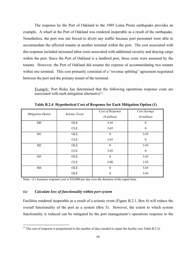
68
The response by the Port of Oakland to the 1989 Loma Prieta earthquake provides an
example. A wharf at the Port of Oakland was rendered inoperable as a result of the earthquake.
Nonetheless, the port was not forced to divert any traffic because port personnel were able to
accommodate the affected tenants at another terminal within the port. The cost associated with
this response included increased labor costs associated with additional security and draying cargo
within the port. Since the Port of Oakland is a landlord port, these costs were assumed by the
tenants. However, the Port of Oakland did assume the expense of accommodating two tenants
within one terminal. This cost primarily consisted of a “revenue splitting” agreement negotiated
between the port and the primary tenant of the terminal.
Example: Port Risky has determined that the following operations response costs are associated with each mitigation alternative53:
Table B.2.4 Hypothetical Cost of Response for Each Mitigation Option (1)
Mitigation Option Seismic Event Cost of Response
($ million)
Cost Savings
($ million)
M0 OLE 3.65 0
CLE 3.65 0
M1 OLE 0 3.65
CLE 3.65 0
M2 OLE 0 3.65
CLE 3.65 0
M3 OLE 0 3.65
CLE 2.00 1.65
M4 OLE 0 3.65
OLE 0 3.65
Note: (1) Assumes response cost is $10,000 per day over the duration of the repair time.
(c) Calculate loss of functionality within port system
Facilities rendered inoperable as a result of a seismic event (Figure B.2.1, Box 4) will reduce the
overall functionality of the port as a system (Box 5). However, the extent to which system
functionality is reduced can be mitigated by the port management’s operations response to the
53 The cost of response is proportional to the number of days needed to repair the facility (see Table B.2.3).

69
emergency (Box 6), for instance, by “doubling up” cargo at wharves that remain functional.
Thus, effective system functionality loss may be considerably smaller than initial system
functionality loss. This step requires estimating the loss of system functionality that would occur
in each of the seismic events identified in Section B.2.2.2 above for each of the mitigation
options identified in Section B.2 2.3 above.
Initial system functionality loss for the seismic events can be estimated as the normal
annual cargo volume handled at the damaged facility relative to the normal annual cargo volume
handled at the port as a whole. It should be measured in percentage terms.
Effective system functionality loss should be estimated by port managers after taking into
account the port’s ability to handle extra cargo at undamaged facilities in the event of a disaster.
This ability will be constrained by factors such as the physical layout of facilities at the port,
contractual arrangements with port tenants, current capacity of the port, and excess capacity at
the time of the disaster. While this ability will vary across facilities, ports, and situations, it is
interesting to note that based on its experiences in the 1989 Loma Prieta earthquake, the Port of
Oakland estimates that it could handle up to roughly 20% loss of initial functionality by
“doubling up” or implementing similar responses. If data and models are available, effective
system functionality loss can be more rigorously evaluated by developing a queuing model that
could simulate the absorption of displaced cargo by undamaged facilities at the port.
Example: Port Risky handles 2 million TEU (twenty-foot equivalent units) of container cargo each year. Some 10% of this cargo will be handled at Wharf X. Since Port Risky operates 365 days a year, this amounts to 200,000 TEU/year or 548 TEU/day handled at Wharf X. If Wharf X were rendered inoperable in an earthquake, initial system functionality loss would be 10%. However, port management believes that in an emergency situation, up to 5% of cargo at the port could be accommodated by “doubling-up” at an undamaged wharf in an adjacent berth. Therefore, if Wharf X were rendered inoperable, effective functionality loss would be 5% (= 10% - 5%). The effective daily loss of cargo in this situation would be 274 TEU/day. Note that in this example, in the interest of simplicity, it is assumed that no other facilities at the port are damaged in an earthquake. However, a complete analysis would evaluate port system functionality by expanding the scope of analysis to include the seismic vulnerability of other facilities at the port.

70
(d) Calculate short-term loss of revenue
Reduction in port functionality (Figure B.2.1, Box 5) will lead to a reduction in cargo traffic at
the port (Box 8). However, the extent of traffic reduction will also be determined by the external
business environment, specifically, by market structure factors such as the prevalence of
discretionary traffic at the port and competition with other ports (Box 7). Reduction in cargo
traffic at the port will lead to loss of port revenues (Box 9), the extent of which will depend upon
the port’s revenue structure (Box 10), that is, its contractual agreements with its users or tenants.
For example, if the majority of a port’s revenue derives from wharfage fees, assessed on a per-
container basis, then loss of cargo could have a direct and significant impact on port revenue.
It is also important to account for sources of new revenue deriving from disaster cost
recovery (Box 11), in particular, insurance claims and disaster assistance from government
agencies such as the Federal Emergency Management Agency (FEMA). There may be
considerable uncertainty associated with the extent of disaster assistance and the time lag before
it becomes available.
We distinguish between short-term and long-term loss of revenue. The latter is discussed
in the next step, below. For present purposes, short-term revenue losses are those experienced
during the time that repairs are being made. Long-term loss consists of business that does not
return to the port even after repairs are completed. Short-term loss is estimated as the effective
loss of traffic multiplied by unit revenue.
Example: Analysis in Section B.2.3.2 (c) above has indicated that Port Risky would lose 5% of its cargo while Wharf X is inoperable, or 274 TEU per day. Port Risky earns $40 per TEU of container cargo that it handles. For mitigation option M0 (no mitigation) in an OLE event, Wharf X would be inoperable for 365 days, whereas with option M1 in the same event, it would be down for 0 days. Accordingly, short-term revenue loss for M0 and M1, respectively, is calculated as follows:
M0: Loss = (365 days) x (274 TEU/day) x (40 $/TEU) = $4.0 million
M1: Loss = (0 days) x (274 TEU/day) x (40 $/TEU) = $0
Cost savings = $4.0 million

71
Table B.2.5 Short-Term Loss of Revenue Associated with Each Mitigation Option
Mitigation Option Seismic Event Short-Term Loss of
Revenue ($ million) Cost Savings($ million)
M0 OLE 4.0 0
CLE 4.0 0
M1 OLE 0 4.0
CLE 4.0 0
M2 OLE 0 4.0
CLE 4.0 0
M3 OLE 0 4.0
CLE 2.2 1.8
M4 OLE 0 4.0
CLE 0 4.0
(e) Calculate long-term loss of business
Loss of port functionality that cannot be compensated for by operations response will cause
cargo to be diverted to a competing port for a time. Generally, local or non-discretionary cargo,
as identified in Section B.2.1.1(c) above, will return as soon as it can be accommodated at the
port. However, non-local or discretionary cargo is at risk of being permanently lost to a
competitor. It is assumed that the longer the period of diversion (i.e., downtime at the damaged
facility), the greater the risk of long-term loss of port business. The actual relationship between
estimated repair time and long-term business loss is an empirical relationship that the port will
need to specify. Similarly, the rate at which lost business is regained after repairs are completed
will also need to be specified by the port. The port’s marketing division may be helpful in
arriving at these estimates.
Example: As noted earlier, 70% of the container cargo handled at Port Risky is discretionary and consists of intermodal cargo that is transported by rail and sea. It is assumed here that this same percentage applies to Wharf X alone. Based on experiences of ports in other recent disasters, port management estimates that where damage is severe enough to put Wharf X out of operation for over 3 months, shipping lines may decide to invest in new arrangements with a competing port and not return. However, if damage is less severe and they can be assured that Wharf X will be functional in 90 days or less, the shippers will agree to interim arrangements at Port Risky, such as berth sharing. Thus in

72
an OLE event, mitigation option M0 (no mitigation), with a 365-day estimated downtime at Wharf X. Long-term loss of revenue could be estimated as follows:
M0: Long-term loss of revenue
= (274 TEU/day) x (40 $/TEU) x (70% discretionary) x (365 days/year)
= $2.8 million per year
M1: Long-term loss of revenue = $0
Cost savings = $2.8 million per year
Table B.2.6 Long-Term Loss of Revenue Associated with Each Mitigation Option
Mitigation
Option
Seismic
Event
Gross Long-
Term Loss of
Revenue
($ million/year)
Gross Annual
Savings
($ million/year)
Total Gross
Savings(1)
($ million)
Total Net
Savings(2)
($ million)
M0 OLE 2.8 0 0 0
CLE 2.8 0 0 0
M1 OLE 0 2.8 40.0 36.0
CLE 2.8 0 0 0
M2 OLE 0 2.8 40.0 36.0
CLE 2.8 0 0 0
M3 OLE 0 2.8 40.0 36.0
CLE 2.8 0 0 0
M4 OLE 0 2.8 40.0 36.0
CLE 0 2.8 0 36.0
Notes: (1) Present value of total stream of annual savings (indefinitely into the future); (2) Total gross savings (for long-term revenue loss) less savings for short-term revenue loss.
The fourth column of Table B.2.6 indicates savings in long-term revenue loss on an annual basis. In order to reflect revenue losses in future years, the fifth column of the table converts annual savings to total savings in present value terms. This is done by dividing the long-term loss of revenue by the discount rate, in this case, 7% (discussed below). Here, it is assumed that long-term revenue losses would never be recovered. The final column of the table adjusts gross long-term savings to net savings by subtracting short-term revenue loss savings (Table B.2.5). This is to avoid double-counting.
73
B.2.4 STEP 4: VALUATE THE BENEFITS AND COSTS OF EACH OF THE PROPOSED MITIGATION OPTIONS
In general, benefits and costs in a social analysis consist of (1) consumer and producer surpluses
through changes in prices; (2) changes in these surpluses through changes in amounts of
unpriced goods (externality effects); and (3) changes in net government revenues. Since we
adopt, for present purposes, the perspective of the port, the analysis may be simplified. We
simply examine changes in the cash flows to the port deriving from implementing a particular
mitigation measure and implementing no mitigation measure. Where they are positive, such as
reductions in future losses, they are benefits; where negative, such as expenditures for mitigation,
they are costs.
The cash flows associated with benefits and costs will occur over time. For example,
benefits will occur sometime in the future after the mitigation costs are incurred. A comparison
can be made by taking into account the time value of money as determined by the discount rate.
This requires the choice of a discount rate and a treatment of how far in the future the benefits
will be realized. (See Appendix A: Discount Rate). The relevant discount rate from the port’s
perspective is simply the rate the port itself uses for financial evaluation.
In this analysis, benefits are considered probabilistic for two reasons. First, the
probability of a seismic event will determine the probability of there being benefits, and this will
vary by the expected magnitude of the seismic event. Therefore, the benefits from mitigation
will, in part, depend on the life span of the proposed facility. The greater the life span, the
greater the probability of a seismic event and the greater the expected value of benefits. Second,
even for a specific level of seismic event and a given level of mitigation, there will also be
uncertainty associated with the magnitude of each benefit category, such as facility repair costs.
For example, each future year will have some probabilistic benefit. This probabilistic benefit will
itself be the mean of a probability distribution that depends on the distribution of repair costs.
One approach is to discount the probabilistic benefits for each year. A simpler approach is to
take the median value of the probability distribution and treat all benefits as occurring at that
point with a cumulative probability representing the total probability of the event over the life of
the facility.
The process described in Sections B.2.3 and B.2.4 can be illustrated and illuminated
through use of a decision tree (Figure B.2.2). A decision tree shows decisions points (decision
nodes) and probable consequences (probability nodes). For a given mitigation decision (Mi),

74
there will be probabilities associated with various levels of seismic events (Ei). The probabilities
sum to one, since “no earthquake” (E0), is part of the probable outcomes. For each given level of
mitigation (Mi) and magnitude of seismic event (Ei), there will be several probable levels of
damage to facilities54 (Di). Again, these probabilities sum to one, since no damage (D0) is a
possibility. For each given level of damage (Di), there will be repair costs (Ri). The repair costs
themselves are also probabilistic, depending on the time value of money and expected unit cost.
A Monte Carlo simulation procedure can be used to handle the required calculations.
M1
M2
M3M4 etc.
E2
E1
E0*M0*
p0e
p1e
p2e
p0d=1
p1d
p2d
D0*
D1
D2
p3d
p4d
D3
D4
p0r R0*
etc.
p1r
p2r
R1
R2
Mi = ith level of mitigationEi = ith magnitude of earthquakeDi = ith magnitude of damageRi = ith magnitude of repair cost
Mi = ith level of mitigationEi = ith magnitude of earthquakeDi = ith magnitude of damageRi = ith magnitude of repair cost
*M0=no mitigation, E0=no earthquake, D0=no damage, R0=no repair cost
Mitigation
Figure B.2.2 Probabilistic Valuation Model
Example: Port Risky uses a 7% nominal discount rate, and assumes a 50-year facility life span, in order to value the benefits and costs of the seismic mitigation options being considered for Wharf X.
54This analysis uses the damage state in order to assess the number of days needed to repair the facility (see Table
B.2.3).

75
In order to calculate the present value of the benefits, the total amount of accrued savings needs to be calculated. This simple procedure is accomplished by adding together the cost savings (Tables B.2.3-B.2.36) for each mitigation option for each seismic event. For example, for mitigation M1, in the event of an OLE, the total cost saving is the sum of the cost savings for repair cost (Table B.2.3), cost of response (Table 4), short-term revenue loss (Table B.2.5) and long term revenue loss (Table B.2.6). Therefore, the total savings accrued in the OLE event as a result of implementing M1 is $47.75 million, which is equal to $4.1 million (repair savings) plus $3.65 million (cost of response savings) plus $4.0 million (short-term revenue loss savings) plus $36.0 million (net long-term loss of revenue savings). This assumes that lost business will never return or be replaced. If it is determined that business will return or be replaced within a specified time period, this calculation can be easily modified. Total benefits are shown in the third column of Table B.2.7 below.
Table B.2.7 Calculation of Expected Value of Benefits of Each Mitigation Option
Mitigation Option Seismic Event Total Benefits
($ million)
Probability of
Event(1)
Expected Value of
Benefits ($)
M0 OLE 0 .01173 0
CLE 0 .00217 0
M1 OLE 47.75 .01173 559,000
CLE 2.81 .00217 6,000
M2 OLE 47.75 .01173 559,000
CLE 3.75 .00217 8,000
M3 OLE 47.75 .01173 559,000
CLE 7.46 .00217 16,000
M4 OLE 47.75 .01173 559,000
CLE 50.25 .00217 111,000
Note: (1) Probability of exceedance. In the case of the OLE, this is net of the probability of exceedance for the CLE.
In Table B.2.7, total benefits are converted to expected values by multiplying by the respective probabilities of exceedance for the event. As shown in Table B.2.1 above, the annual probability of exceedance for the CLE (0.40g) is 0.00217. For the OLE (0.15g), the Table 1 probability is 0.01390. The CLE probability is subtracted from this value to yield a net exceedance probability for the OLE for use in Table B.2.7 (0.01173 = 0.01390 – 0.00217). This is done to avoid double-counting.
The next step involves calculating the present value of the expected benefits. This is done dividing the expected value of the benefits by (1+r)n, where r is the discount rate and n is the year in which the benefit is realized. As was discussed above, the discount

76
rate is .07. The calculation is carried out over the entire life span of the proposed facility, in this case 50 years. For example, for the M1 event:
Table B.2.8 Calculation of Present Value for the M1 Mitigation Option
Year (n)
Expected
Value OLE
($)
Expected
Value CLE
($)
(1+r)n
Present
Value OLE
($)
Present
Value CLE
($)
Sum PV ($)
1 559,000 6,000 1.07 522,430 5,607 528,037
2 559,000 6,000 1.14 488,252 5,241 493,493
3 559,000 6,000 1.23 456,311 4,898 461,208
4 559,000 6,000 1.31 426,458 4,577 431,036
5 559,000 6,000 1.40 398,559 4,278 402,837
6 ........... … … … … … …
.............. 50 … … … … … …
Sum PV Year
1-50
7,797,422
Costs - 400,000
NPV
7,397,422
The present value of the benefits associated with each event, OLE and CLE, is summed in order to obtain the present value of the benefits for each year.
B.2.5 STEP 5: CHOOSE BETWEEN ALTERNATIVE MITIGATION OPTIONS
Several different criteria are used in financial evaluation. These include (1) net-present value,
(2) benefit-cost ratios, (3) internal rates of return, and (4) pay-back periods. Our treatment will
proceed in terms of net present value (NPV) and the internal rate of return (IRR). The NPV is
most widely used in academic analysis and the IRR is commonly used in the private sector. Due
to deficiencies in the IRR, occasionally it produces an incorrect result, which is different from
the result obtained from the NPV.
Example: The net present value is calculated by summing the present value of the benefits for each year of the life of the facility and then subtracting out the cost of the mitigation (see Table B.2.8 above). Performing this calculation for each of the mitigation options produces the following distribution of NPVs:

77
Table B.2.9 Distribution of NPVs for Each Mitigation Option
Mitigation Option NPV
($ million)
Meets Performance
Criterion 1?
Meets Performance
Criterion 2?
M0 0 No No
M1 7.4 Yes No
M2 5.7 Yes No
M3 5.8 Yes Yes
M4 2.7 Yes Yes
The option that maximizes the net present value is M1. If the port’s objective is to select the most cost-effective option, it would choose M1. However, as indicated in Table B.2.9, while option M1 meets Performance Criterion 1 (Section B.2.2.2 above), it does not meet Performance Criterion 2. The mitigation option that maximizes net present value while meeting both performance criteria is option M3.

78
References for Appendix B
Chang, S. 2000. Disasters and transport systems: Loss, recovery, and competition at the Port of Kobe after the 1995 earthquake. Journal of Transport Geography 8(1): 53-65. Eidinger, J., and E. Avila (Eds.). 1998. Guidelines for the Seismic Upgrade of Existing Water Transmission Facilities. ASCE: Reston, VA.
FEMA. 1994. Seismic Rehabilitation of Federal Buildings: A Benefit/Cost Model, Volumes 1 and 2. FEMA: Sacramento, CA.
Hershman, M. (Ed). 1988. Urban Ports and Harbor Management. Taylor and Francis: New York, NY.
Port of Oakland. 1999. Request for Proposals for Wharf and Embankment Strengthening Program. Port of Oakland: Oakland, CA.
Slovic, P., B. Fishoff, and S. Lichtenstein. 1980. Facts and fear: Understanding perceived risk, in Schwing and Albers (Eds.), Social Risk Assessment: How Safe is Safe Enough?, 181-214. Plenum Press: New York, NY. Taylor, C., S. Werner, et al. 1995. Proposed POLA 2020 Acceptable Seismic Risk Procedure with Demonstration Application to Pier 300 Wharf. Dames and Moore: San Francisco, CA. Werner. S. (ed.) 1998. Seismic Guidelines for Ports. ASCE: Reston, VA. __________, and S. Dickenson, and C. Taylor. 1997. Seismic risk reduction at ports: Case studies and acceptable risk evaluation. Journal of Waterway, Port, Coastal, and Ocean Engineering 123(6): 337-346. Zerbe, R., and D. Dively. 1994. Benefit-Cost Analysis In Theory and Practice. Harper Collins: New York, NY.
79
References
Arrow, Kenneth. 1951. “Little’s Critique of Welfare Economics.” American Economic Review 41(5): 923-934. Baltimore Gas & Electric Co. v. Natural Resources Defense Council, Inc., 462 U.S. 87, 76 L. Ed. 2d 437, 103 S. Ct. 2246, 1983 U.S. LEXIS 48, 51 U.S.L.W. 4678. Pub. Util. Rep.4th (PUR) 501. Boadway, Robin W. and N. Bruce. 1984. Welfare Economics. New York: Basil Blackwell. Bradford, D.F., 1975. “Constraints on Government Investment Opportunities and the Choice of Discount Rate.” American Economic Review 65: 887-899. Brealey, R. and Myers, S. 1988. Principles of Corporate Finance, Third Edition, New York: McGraw-Hill, Inc Chang, SE, M. Shinozuka, and D.B. Ballantyne. 1998. “Life Cycle Cost Analysis with Natural Hazard Risk: A Framework and Issues for Water Systems,” in Optimal Performance of Civil Infrastructure Systems: 58-73. Edited by D. Frangopol. Reston, VA: American Society of Civil Engineers. Chang, S.E. and M. Shinozuka. 1996. “Life-Cycle Cost Analysis with Natural Hazard Risk, ” ASCE Journal of Infrastructure Systems 2 (3): 118-126. Chipman, John. 1987. “Compensation Principle” in The New Palgrave: A Dictionary of Economics: 524-531. Edited by John Eatwell, Murrary Milgate, Peter Newman. Vol. 1. Coleman, Jules 1980. “Efficiency, Utility, and Wealth Maximization.” Hofstra Law Review. 8(3): 509-551. Cornell, C.A. and H. Krawinkler. 2000. “Progress and Challenges in Seismic Performance Assessment,” PEER Center News 3(2). Cropper, M.L. and P.R. Portney. 1990. “Discounting and the Evaluation of Lifesaving Programs”, Journal of Risk and Uncertainty, 3: 369-379. Cullen, A.C., Frey, H.C., 1999. Probabilistic Techniques in Exposure Assessment: A Handbook for Dealing with Variability and Uncertainty in Models and Inputs. Plenum Press: New York.
80
Dively, Dwight, and Richard Zerbe, 1991. “The Discount Rate Policy for Municipalities.” Working Paper. Dupuit, Arsene J.E., 1844. “On the Measurement of the Utility of Public Works.” (trans., 1952, IEP) Annales des Ponts et Chaussees 8: 332-375. Farrow, Scott, 2000. “Using Risk Assessment, Benefit-Cost Analysis, and Real Options to Implement a Precautionary Principle.” Working Paper. Farrow, Scott, R. Ponce, E. Wong, E. Faustman, and R. Zerbe, 2001. “Facilitating Regulatory Design and Stakeholder Participation: The FERET Template with an Application to the Clean Air Act,” in Improving Regulation: Cases in Environment, Health, and Safety. Edited by P. Fischbeck and S. Farrow. Resources for the Future Press: Washington D.C. “Federal Regulation.” Code of Federal Regulations. Title 2, 3, Pt. 128, 1981 ed. Graham, JD (1995). “Edging towards sanity on regulatory risk reform.” Issues in Science and Technology. 61-66. Hahn, Robert W., editor, 1996. Risks, Cost, and Lives Saved: Getting Better Results from Regulation. Oxford University Press: New York. Harberger, Arnold, 1971. “Three Basic Postulates For Applied Welfare Economics Interpretative Essay.” Journal of Economic Literature 9: 785. Hicks, John R. 1939. “The Foundations of Welfare Economics.” Economic Journal 49: 696. Hotelling, Harold, 1938. “The General Welfare in Relation to Problems of Taxation and of Railway and Utility Rates,” Econometrica 6, 242-269. Kind, P., P. Rosser, and A. Williams 1982. “Valuation of Quality of Life: Some Psychometric Evidence. ” in The Value of Life and Safety: 159-170. Edited by. M. W. Jones-Lee. Amsterdam: Elsevier/North Holland, 159-170. Kahneman, Daniel and Amos Tversky. 1979. “Prospect Theory: An Analysis Of Decision Under Uncertainty.” Econometrica 47 (2): 263-91. Kaldor, Nicholas. 1939. “Welfare Propositions In Economics and Inter-Personal Comparisons Of Utility.” Economic Journal 49: 549. Kunreuther, Howard and Douglas Easterling. 1992. “Are Risk-Benefit Tradeoffs Possible In Siting Hazardous Facilities?” American Economic Review 80(2): 252-256 Lave, Lester, 1996. “BCA: Do the Benefits Exceed the Costs,” in Risks, Costs and Lives Saved. Edited by R. Hahn. New York: Oxford University Press Lesser, Jon and R. O. Zerbe Jr., 1998. “A Practitioner’s Guide To BCA” in The Handbook of Public Finance. Edited by Fred Thompson and Mark Green. New York: Marcel Drekker.

81
Lind, R.C. 1982. “A Primer on the Major Issues Relating to the Discount Rate for Evaluating National Energy Options,” in Discounting for Time and Risk in Energy Policy. Edited by R.C. Lind John Hopkins Press for Resources for the Future, Baltimore, MD. Marshall, A., 1890. Principles of Economics. 8th Edition 1920, Macmillan: London. Mishan, Ezra J., 1952. “The Principle of Compensation Reconsidered.” The Journal of Political Economy 60(4): 312-322. Office of Management and Budget, 1992. “Guidelines and Discount Rates for Benefit-Cost Analysis of Federal Programs.” Circular No. A-94. Pacific Gas & Electric Co. v. State Energy Resources Conservation & Dev. Com., 461 U.S. 190, 75 L. Ed. 2d 752, 103 S. Ct. 1713, 1983 U.S. LEXIS 25, 51 U.S.L.W. 4449. Parfit, Derek. 1992. “An Attack On The Social Discount Rate.” in Values and Public Policy. Edited by Claudia Mills. Fort Worth: Harcourt Brace Javanovich. Parfit, Derek. 1994. “The Social Discount Rate” in Politics Of The Environment. Edited by R. E. Goodwin. Aldershot: Edward Elgar. Pearce, David, A. Markandya and E. Barbier, 1989. Blueprint for a Green Economy. Earthscan Publications: London Pildes, Richard and Cass Sunstein (1995). “Reinventing the Regulatory State.” University of Chicago Law Review. 62: 1-129. Plater, Zgymunt, J. B. Robert, H. Abrams, W. Goldfarb and R. L. Graham. 1998. Environmental Law and Policy: Nature, Law, and Society. St. Paul: West Publishing Co. Port of Oakland. 1999. Request for Proposals for Wharf and Embankment Strengthening Program. Port of Oakland: Oakland, CA. Portney, Paul and John P. Weyant. (editors) 1999. Discounting and Intergenerational Equity. Washington D. C.: Resources For The Future. Posner, Richard. 1985. “An Economic Theory of the Criminal Law.” Columbia Law Review 85: 1193. Posner, Richard. 1987. “The Justice of Economics.” Economic Delle Schelte Pubbliche. 1: 1. Rauch, James E., 1995. “Bureaucracy, Infrastructure, and Economic Growth: Evidence from U.S. Cities During the Progressive Era.” American Economic Review 85: 968-979. “Regulatory Planning and Review.” Code of Federal Regulations. Title 3, Pt. 638, 649, 1993 ed. “Regulatory Planning Process.” Code of Federal Regulations. Title 3, Pt. 323, 1985 ed.

82
Robbins, Lionel .1938. “Interpersonal Comparisons of Utility: a Comment.” Economic Journal 48: 635 Schultze, William D., D. S. Brookshire and T. Sandler. 1981. “The Social Rate of Discount For Nuclear Waste Storage: Economics of Ethics.” Natural Resources Journal 21: 811-832. Scitovsky, Tibor, 1941, “A Note on Welfare Propositions in Economics.” Review of Economic Studies 9: 77-88. Svenson, Ola and G. Karlsson, 1989. “Decision-Making, Time Horizons, and Risk in the Very Long Term Perspective.” Risk Analysis 9: 385-398. Taylor, C., S. Werner, et al. 1995. Proposed POLA 2020 Acceptable Seismic Risk Procedure with Demonstration Application to Pier 300 Wharf. Dames and Moore: San Francisco, CA. Tengs, Tammy O., and JD Graham, 1996. “The Opportunity Costs of Haphazard Social Investments in Life-Saving” in Risks, Costs, and Lives Saved. Edited by Robert W. Hahn. Oxford University Press: New York. United States Congress. 1995 US HB. 1022 (SN). “The Risk Assessment and Cost Benefit Act of 1995.” Passed House on February 28, 1995. Wasankari, Brian, Richard O. Zerbe Jr. and Steven Vinyard, 2000. “On Distributive Justice and Economic Efficiency: An Integrated Theory of the Common Law.” Research in Law and Economics 19, pp. 139-222. Werner, S., S. Dickenson, and C. Taylor. 1997. Seismic risk reduction at ports: Case studies and acceptable risk evaluation. Journal of Waterway, Port, Coastal, and Ocean Engineering 123(6): 337-346. Whittington, Dale and Duncan Macrae Jr. 1986 “The Issue of Standing in BCA.” Journal of Policy Analysis and Management, 9(2) pp. 201-218. Zerbe, Richard O. Jr. 2002, “Whose Values Count in Economic Analysis? ” Research in Law and Economics. __________. 2001. Efficiency in Law and Economics, Aldershot England: Edward Elgar. __________. 2000. “What is Economic Efficiency: A New Paradigm,” working paper. __________. 1998a. “An Integration of Equity and Efficiency.” Washington Law Review 73(April): 349-361. __________. 1998b. “Is Cost-Benefit Analysis Legal? Three Rules.” Journal of Policy Analysis and Management 17(3): 419-456.

83
_________. 1991. “Comment: Does BCA Stand Alone? Rights and Standing.” Journal of Policy Analysis and Management 10(1): 96-105. __________. and D. Dively, 1994. Benefit Cost Analysis in Theory and Practice. Harper Collins: New York. __________. and H. McCurdy 1999. “The Failure of Market Failure.” Journal of Policy Analysis and Management. 18(4): 558-578.