package ‘cna’ - r · package ‘cna ’ june 13, 2018 type ... ness, and a test for structural...

Package ‘cna’June 13, 2018

Type Package

Title Causal Modeling with Coincidence Analysis

Version 2.1.1

Date 2018-06-13

Description Provides comprehensive functionalities for causal modeling with Coincidence Analy-sis (CNA), which is a configurational comparative method of causal data analysis that was first in-troduced in Baumgartner (2009) <doi:10.1177/0049124109339369>. CNA is related to Qualita-tive Comparative Analysis (QCA), but contrary to the latter, it is custom-built for uncover-ing causal structures with multiple outcomes and it builds causal models from the bot-tom up by gradually combining single factors to complex dependency structures until the re-quested thresholds of model fit are met. The new functionalities provided by this package ver-sion include various new parameters of model fit, as exhaustiveness and faithful-ness, and a test for structural redundancies in multi-outcome models with a corresponding func-tion that eliminates such redundancies. Also, the algorithmic efficiency has been significantly in-creased. Finally, the package now comes with an extensive vignette.

License GPL (>= 2)

URL https://CRAN.R-project.org/package=cna

Depends R (>= 3.2.0)

Imports Rcpp, utils, stats, matrixStats

LinkingTo Rcpp

Suggests dplyr

NeedsCompilation yes

LazyData yes

Author Mathias Ambuehl [aut, cre, cph],Michael Baumgartner [aut, cph],Ruedi Epple [ctb],Alrik Thiem [ctb]

Maintainer Mathias Ambuehl <[email protected]>

Repository CRAN

Date/Publication 2018-06-13 10:02:55 UTC

1

https://CRAN.R-project.org/package=cna

2 cna-package

R topics documented:cna-package . . . . . . . . . . . . . . . . . . . . . . . . . . . . . . . . . . . . . . . . . 2allCombs . . . . . . . . . . . . . . . . . . . . . . . . . . . . . . . . . . . . . . . . . . 4cna . . . . . . . . . . . . . . . . . . . . . . . . . . . . . . . . . . . . . . . . . . . . . . 5coherence . . . . . . . . . . . . . . . . . . . . . . . . . . . . . . . . . . . . . . . . . . 17condition . . . . . . . . . . . . . . . . . . . . . . . . . . . . . . . . . . . . . . . . . . 19condTbl . . . . . . . . . . . . . . . . . . . . . . . . . . . . . . . . . . . . . . . . . . . 24d.autonomy . . . . . . . . . . . . . . . . . . . . . . . . . . . . . . . . . . . . . . . . . 27d.educate . . . . . . . . . . . . . . . . . . . . . . . . . . . . . . . . . . . . . . . . . . 28d.irrigate . . . . . . . . . . . . . . . . . . . . . . . . . . . . . . . . . . . . . . . . . . . 29d.jobsecurity . . . . . . . . . . . . . . . . . . . . . . . . . . . . . . . . . . . . . . . . . 30d.minaret . . . . . . . . . . . . . . . . . . . . . . . . . . . . . . . . . . . . . . . . . . 30d.pacts . . . . . . . . . . . . . . . . . . . . . . . . . . . . . . . . . . . . . . . . . . . . 31d.pban . . . . . . . . . . . . . . . . . . . . . . . . . . . . . . . . . . . . . . . . . . . . 32d.performance . . . . . . . . . . . . . . . . . . . . . . . . . . . . . . . . . . . . . . . . 32d.volatile . . . . . . . . . . . . . . . . . . . . . . . . . . . . . . . . . . . . . . . . . . 33d.women . . . . . . . . . . . . . . . . . . . . . . . . . . . . . . . . . . . . . . . . . . . 34makeFuzzy . . . . . . . . . . . . . . . . . . . . . . . . . . . . . . . . . . . . . . . . . 34minimalizeCsf . . . . . . . . . . . . . . . . . . . . . . . . . . . . . . . . . . . . . . . . 36selectCases . . . . . . . . . . . . . . . . . . . . . . . . . . . . . . . . . . . . . . . . . 38some . . . . . . . . . . . . . . . . . . . . . . . . . . . . . . . . . . . . . . . . . . . . . 40truthTab . . . . . . . . . . . . . . . . . . . . . . . . . . . . . . . . . . . . . . . . . . . 42tt2df . . . . . . . . . . . . . . . . . . . . . . . . . . . . . . . . . . . . . . . . . . . . . 46

Index 48

cna-package cna: A Package for Causal Modeling with Coincidence Analysis

Description

The cna package implements the method of Coincidence Analysis (CNA), which was first intro-duced in Baumgartner (2009a, 2009b, 2013). CNA is a configurational comparative method relatedto Qualitative Comparative Analysis (QCA) (Ragin 1987, 2008). Like QCA, CNA processes con-figurational data, i.e. data consisting of observed cases featuring different factor configurations, itsearches for redundancy-free sufficient and necessary conditions of causally modeled outcomes, itplaces a Boolean ordering over causally relevant factors (instead of quantifying effect sizes in thevein of regression analytic methods), and it draws on the same regularity theoretic notion of causa-tion as QCA, i.e. the notion first introduced by Mackie (1974). Contrary to QCA, however, CNA iscustom-built to treat multiple factors as outcomes, and it does not generate causal models from thetop down by first building maximal Boolean dependency structures and then gradually eliminatingredundant elements (using e.g. Quine-McCluskey optimization; cf. Quine 1959, McCluskey 1965);rather, CNA builds causal models from the bottom up by gradually combining single factors tocomplex dependency structures until the requested thresholds of model fit are met, such that the re-sulting models are automatically redundancy-free. As a consequence of these differences, CNA canidentify common-cause and causal-chain structures and it can avoid the task of redundancy elim-ination (which creates various problems for QCA). Moreover, the algorithm does not require an

cna-package 3

input identifying the endogenous factors; it can infer that from the data. Finally, data fragmentation(limited diversity) does not force CNA to resort to counterfactual reasoning.

The new functionalities provided by this version of the cna package include various model fit pa-rameters measuring, for instance, the degree of correspondance between the configurations that are,in principle, compatible with causal models and the configurations actually contained in the data.Moreover, multi-outcome models are now tested for structural redundancies and a new function hasbeen added that eliminates such redundancies. Also, algorithmic efficiency has been significantlyincreased. Finally, the package now comes with an extensive vignette that presents the theoreticalbackground of CNA and introduces to causal modeling with cna on the basis of many concreteexamples.

Details

Package: cnaType: PackageVersion: 2.1.1Date: 2018-06-13License: GPL (>= 2)

Author(s)

Authors:Mathias Ambuehl<[email protected]>

Michael BaumgartnerDepartment of PhilosophyUniversity of Bergen<[email protected]>

Maintainer:Mathias Ambuehl

References

Baumgartner, Michael. 2009a. “Inferring Causal Complexity.” Sociological Methods & Research38(1):71-101.

Baumgartner, Michael. 2009b. “Uncovering Deterministic Causal Structures: A Boolean Ap-proach.” Synthese 170(1):71-96.

Baumgartner, Michael. 2013. “Detecting Causal Chains in Small-n Data.” Field Methods 25 (1):3-24.

Baumgartner, Michael, and Ruedi Epple. 2014. “A Coincidence Analysis of a Causal Chain: TheSwiss Minaret Vote.” Sociological Methods & Research 43(2):280-312.

Baumgartner, Michael and Alrik Thiem. 2015. “Identifying Complex Causal Dependencies inConfigurational Data with Coincidence Analysis”, The R Journal 7:176-184.

4 allCombs

Mackie, John L. 1974. The Cement of the Universe: A Study of Causation. Oxford: OxfordUniversity Press.

McCluskey, Edward J. 1965. Introduction to the Theory of Switching Circuits. Princeton: PrincetonUniversity Press.

Quine, Willard v. O. 1959. “On Cores and Prime Implicants of Truth Functions.” The AmericanMathematical Monthly 66:755-760.

Ragin, Charles C. 1987. The Comparative Method. Berkeley: University of California Press.

Ragin, Charles C. 2008. Redesigning Social Inquiry: Fuzzy Sets and Beyond. Chicago: Universityof Chicago Press.

allCombs Generate all possible value configurations of a given set of factors

Description

Generates a data frame of all possible value configurations of length(x) multi-valued factors, thefirst factor having x[1] values, the second x[2] values etc. The factors are labeled using capitalletters.

Usage

allCombs(x)

Arguments

x integer vector with values >0

Details

In combination with selectCases and makeFuzzy, allCombs is useful for simulating data, whichare needed for inverse search trials that assess the correctness of models output by cna. In a nutshell,allCombs generates the space of all logically possible configurations of the factors in an analyzedfactor set, selectCases selects those configurations from this space that are compatible with agiven data-generating causal structure, and makeFuzzy introduces noise into that data.

Value

A data frame.

See Also

selectCases, makeFuzzy

cna 5

Examples

# Generate all logically possible configurations of 5 dichotomous factors named "A", "B",# "C", "D", and "E".allCombs(c(2, 2, 2, 2, 2)) - 1# allCombs(c(2, 2, 2, 2, 2)) generates the value space for values 1 and 2, but as it is# conventional to use values 0 and 1 for Boolean factors, 1 must be subtracted from# every value output by allCombs(c(2, 2, 2, 2, 2)) to yield a Boolean data frame.

# Generate all logically possible configurations of 5 multi-value factors named "A", "B",# "C", "D", and "E", such that A can take on 3 values {1,2,3}, B 4 values {1,2,3,4},# C 3 values etc.dat0 <- allCombs(c(3, 4, 3, 5, 3))head(dat0)nrow(dat0) # = 3*4*3*5*3

# Generate all configurations of 5 dichotomous factors that are compatible with the causal# chain (A*b + a*B <-> C)*(C*d + c*D <-> E).dat1 <- allCombs(c(2, 2, 2, 2, 2)) - 1(dat2 <- selectCases("(A*b + a*B <-> C)*(C*d + c*D <-> E)", dat1))

# Generate all configurations of 5 multi-value factors that are compatible with the causal# chain (A=2*B=1 + A=3*B=3 <-> C=1)*(C=1*D=2 + C=4*D=4 <-> E=3).dat1 <- allCombs(c(3, 3, 4, 4, 3))dat2 <- selectCases("(A=2*B=1 + A=3*B=3 <-> C=1)*(C=1*D=2 + C=4*D=4 <-> E=3)", dat1,

type = "mv")nrow(dat1)nrow(dat2)

# Generate all configurations of 5 fuzzy-set factors that are compatible with the causal# structure A*b + C*D <-> E, such that con = .8 and cov = .8.dat1 <- allCombs(c(2, 2, 2, 2, 2)) - 1dat2 <- makeFuzzy(dat1, fuzzvalues = seq(0, 0.45, 0.01))(dat3 <- selectCases1("A*b + C*D <-> E", con = .8, cov = .8, dat2))

# Inverse search for the data generating causal structure A*b + a*B + C*D <-> E from# fuzzy-set data with non-perfect consistency and coverage scores.dat1 <- allCombs(c(2, 2, 2, 2, 2)) - 1dat2 <- makeFuzzy(dat1, fuzzvalues = 0:4/10)set.seed(3)dat3 <- selectCases1("A*b + a*B + C*D <-> E", con = .8, cov = .8, dat2)fscna(dat3, ordering = list("E"), strict = TRUE, con = .8, cov = .8)

cna Perform Coincidence Analysis

Description

The cna function performs Coincidence Analysis to identify atomic solution formulas (asf) consist-ing of minimally necessary disjunctions of minimally sufficient conditions of all outcomes in the

6 cna

data and combines the recovered asf to complex solution formulas (csf) representing multi-outcomestructures, e.g. common-cause and/or causal-chain structures.

Usage

cna(x, type, ordering = NULL, strict = FALSE, con = 1, cov = 1, con.msc = con,notcols = NULL, rm.const.factors = TRUE, rm.dup.factors = TRUE,maxstep = c(3, 3, 9), inus.only = FALSE, only.minimal.msc = TRUE,maxSol = 1e6, suff.only = FALSE, what = if (suff.only) "m" else "ac",cutoff = 0.5, border = c("down", "up", "drop"), details = FALSE)

cscna(...)mvcna(...)fscna(...)

## S3 method for class 'cna'print(x, what = x$what, digits = 3, nsolutions = 5,

details = x$details, show.cases = NULL, ...)

Arguments

x A data frame or an object of class “truthTab” (as output by truthTab).

type A character vector specifying the type of x: "cs" (crisp-set), "mv" (multi-value),or "fs" (fuzzy-set).

ordering A list of character vectors specifying the causal ordering of the factors in x.

strict Logical; if TRUE, factors on the same level of the causal ordering are not potentialcauses of each other; if FALSE, factors on the same level are potential causes ofeach other.

con Numeric scalar between 0 and 1 to set the minimum consistency threshold ev-ery minimally sufficient condition (msc), atomic solution formula (asf), andcomplex solution formula (csf) must satisfy. (See also the argument con.mscbelow).

cov Numeric scalar between 0 and 1 to set the minimum coverage threshold everyasf and csf must satisfy.

con.msc Numeric scalar between 0 and 1 to set the minimum consistency threshold everymsc must satisfy. Allows for imposing a consistency threshold on msc thatdiffers from the value con imposes on asf and csf. Defaults to con.

maxstep Vector of three integers; the first specifies the maximum number of conjuncts ineach disjunct of an asf, the second specifies the maximum number of disjunctsin an asf, the third specifies the maximum complexity of an asf. The complexityof an asf is an integer defined to be the sum of the number of conjuncts in all ofits disjuncts, i.e. the total number of exogenous factors in the asf.

inus.only Logical; if TRUE, only disjunctions satisfying the INUS criteria are retained asasf. Defaults to FALSE.

only.minimal.msc

Logical; if TRUE (the default), only minimal conjunctions are retained as msc.If FALSE, sufficient conditions are not required to be minimal, in which case thenumber of msc will usually be much greater.

cna 7

maxSol Maximum number of asf calculated.

suff.only Logical; if TRUE, the function only searches for msc and does not search for asfand csf.

notcols A character vector of factors to be negated in x. If notcols = "all", all factorsin x are negated.

rm.const.factors, rm.dup.factors

Logical; if TRUE (default), factors with constant values are removed and all butthe first of a set of duplicated factors are removed. These parameters are passedto truthTab.

what A character string specifying what to print; "t" for the truth table, "m" for msc,"a" for asf, "c" for csf, and "all" for all. Defaults to "ac" if suff.only = F,and to "m" otherwise.

cutoff Minimum membership score required for a factor to count as instantiated in thedata and to be integrated in the analysis. Value in the unit interval (0,1). Thedefault cutoff is 0.5. Only meaningful if type="fs".

border A character vector specifying whether factors with membership scores equal tocutoff are rounded up ("up"), rounded down ("down") or dropped from theanalysis ("drop"). Only meaningful if type="fs".

details Either TRUE/FALSE, or a character vector with possible elements "inus","exhaustiveness", "faithfulness", "coherence", "redundant". The stringscan also be abbreviated, e.g. "i" for "inus", "e" or "exh" for "exhaustiveness",etc.

digits Number of digits to print in consistency, coverage, exhaustiveness, faithfulness,and coherence scores.

nsolutions Maximum number of msc, asf, and csf to print. Alternatively, nsolutions="all"will print all solutions.

show.cases Logical; if TRUE, the truthTab’s attribute “cases” is printed. See print.truthTab

... In cscna, mvcna, fscna: any formal argument of cna except type. In print.cna:arguments passed to other print-methods.

Details

The first input x of the cna function is a data frame or an object of class “truthTab” as issued bytruthTab. To ensure that no misinterpretations of returned asf and csf can occur, users are advisedto use only upper case letters as factor (column) names. Column names may contain numbers, butthe first sign in a column name must be a letter. Only ASCII signs should be used for column androw names.

cna must be told what type of data x contains, unless x is a truthTab. In the latter case, the typeof x is already defined. Data that feature factors taking values 1 or 0 only are called crisp-set, inwhich case the type argument takes its default value "cs". If the data contain at least one factorthat takes more than two values, e.g. {1,2,3}, the data count as multi-value, which is indicated bytype = "mv". Data featuring at least one factor taking real values from the interval [0,1] countas fuzzy-set, which is specified by type = "fs". (Note that mixing multi-value and fuzzy-setfactors in one analysis is not (currently) supported). To abbreviate the specification of the data typeusing the type argument, the functions cscna(x, ...), mvcna(x, ...), and fscna(x, ...)

8 cna

are available as shorthands for cna(x, type = "cs", ...), cna(x, type = "mv", ...), andcna(x, type = "fs", ...), respectively.

A data frame or truth table x with a corresponding type specification is the only mandatory input ofthe cna function. If no causal ordering is provided (see below), all factors in x are treated as potentialoutcomes; more specifically, in case of "cs" and "fs" data, cna tests for all factors whether theirpresence (i.e. them taking the value 1) can be modeled as an outcome, and in case of "mv" data,cna tests for all factors whether any of their possible values can be modeled as an outcome. That isdone by, first, searching all minimally sufficient conditions (msc) that meet the threshold given bycon.msc (resp. con, if con.msc = con) for each factor in x. Then, cna disjunctively combines thesemsc to minimally necessary conditions that meet the threshold given by cov such that the wholedisjunction meets the threshold given by con. The resulting expressions are the atomic solutionformulas (asf) for every factor that can be modeled as outcome. The default value for con.msc,con, and cov is 1.

[Consistency and coverage measures have originally been introduced into the QCA protocol byRagin (2006). Informally put, consistency reproduces the degree to which the behavior of an out-come obeys a corresponding sufficiency or necessity relationship or a whole causal model, whereascoverage reproduces the degree to which a sufficiency or necessity relationship or a whole modelaccounts for the behavior of the corresponding outcome. As the implication operator underlyingthe notions of sufficiency and necessity is defined differently in classical and in fuzzy logic, the twomeasures are defined differently for crisp-set and multi-value data, on the one hand, and fuzzy-setdata, on the other. For details cf. Ragin (2006).]

cna builds msc and asf from the bottom up. That is, in a first phase, cna checks whether singlefactor values A, b, C, (where "A" stands for "A=1" and "b" for "B=0") or D=3, E=2, etc. (whosemembership scores, in case of "fs" data, meet cutoff in at least one case) are sufficient for anoutcome (where a factor value counts as sufficient iff it meets the threshold given by con.msc).Next, conjuncts of two factor values A*b, A*C, D=3*E=2 etc. (whose membership scores, in caseof "fs" data, meet cutoff in at least one case) are tested for sufficiency. Then, conjuncts of threefactors, and so on. Whenever a conjunction (or a single factor value) is found to be sufficient,all supersets of that conjunction contain redundancies and are, thus, not considered for the furtheranalysis. The result of that first phase is a set of msc for every outcome. To recover certain targetstructures in cases of noisy data, it may be useful to allow cna to also consider sufficient conditionsfor further analysis that are not strictly speaking minimal. This can be accomplished by settingonly.minimal.msc to FALSE. A concrete example illustrating the purpose of only.minimal.mscis provided in the example section below.

In the next phase, minimally necessary disjunctions are built for each outcome by first testingwhether single msc are necessary, then disjunctions of two msc, then of three, etc (where a disjunc-tion of msc counts as necessary iff it meets the threshold given by cov). Whenever a disjunction ofmsc (or a single msc) is found to be necessary, all supersets of that disjunction contain redundanciesand are, thus, excluded from the further analysis. Finally, all and only those disjunctions of mscthat meet both cov and con are issued as redundancy-free asf.

As the combinatorial search space for asf is potentially too large to be exhaustively scanned inreasonable time, the argument maxstep allows for setting an upper bound for the complexity ofthe generated asf. maxstep takes a vector of three integers c(i,j,k) as input, entailing that thegenerated asf have maximally j disjuncts with maximally i conjuncts each and a total of maximallyk factors (k is the maximal complexity). The default is maxstep = c(3,3,9).

Note that the default con and cov thresholds of 1 will often not yield any asf because real-lifedata tend to feature noise due to uncontrolled background influences. In such cases, users should

cna 9

gradually lower con and cov (e.g. in steps of 0.05) until cna finds solution formulas—for the aimof a CNA is to find solutions with the highest possible consistency and coverage scores. con andcov should only be lowered below 0.75 with great caution. If thresholds of 0.75 do not result insolutions, the corresponding data feature such a high degree of noise that there is a severe risk ofcausal fallacies.

If cna finds asf, it combines them to complex solution formulas (csf). Asf with identical outcomesare not combined, for they do not represent a complex causal structure but model ambiguities withrespect to one outcome. Asf with different outcomes can be concatenated to csf using two differentsigns: "*" and ",". If asf1 and asf2 have at least one factor in common, they are combined to "asf1* asf2"; if they have no common factor, they are combined to "asf1, asf2". That is, csf with "*"as main operator represent cohering complex causal structures and the degree of coherence in theanalyzed data is issued as coherence score (cf. coherence). Csf with "," as main operator representnon-cohering structures. For instance, the two asf (D + U <-> L) and (G + L <-> E) can be combinedto the cohering csf "(D + U <-> L) * (G + L <-> E)", which represents a causal chain from D + Uvia L to E, whereas (D + U <-> L) and (G + F <-> E) yield the non-cohering csf "(D + U <-> L),(G + F <-> E)".

The default output of cna lists asf and csf with consistency, coverage, and complexity scores. Butcna can calculate a number of further solution attributes: inus, exhaustiveness, faithfulness,coherence, and redundant, all of which are recovered by setting details to its non-default valueTRUE. These attributes require explication (see also the package vignette).

complexity: Complexity corresponds to the number of exogenous factors in a solution. inus: Thetheory of causation underlying cna is called INUS-theory (Mackie 1974, ch. 3; Baumgartner 2008).Very roughly, it says that X is causally relevant to Y iff X is contained in a minimally necessarydisjunction of minimally sufficient conditions of Y. It was originally designed for noise-free datathat can be modeled with con = cov = 1. It turns out, however, that at consistency and coveragescores below 1 expressions can count as minimally necessary disjunctions of minimally sufficientconditions that, for mere logical reasons, could not possibly count as such at con = cov = 1. inusthus indicates whether or not a solution counts as an INUS solution relative to the strict criteriaimposed by the INUS-theory for the case of con = cov = 1. If the user is only interested in INUSsolutions, the argument inus.only is available; if inus.only = TRUE, only INUS solutions arebuilt.

Exhaustiveness and faithfulness are two measures of model fit that quantify the degree of corre-spondence between the configurations that are, in principle, compatible with a solution and theconfigurations contained in the data from which that solution is derived. Roughly, exhaustivenessis high when all or most configurations compatible with a solution are in the data, whereas faithful-ness is high when no or only few configurations that are incompatible with a solution are in the data.More specifically, exhaustiveness amounts to the ratio of the number of configurations in the datathat are compatible with a solution to the number of configurations in total that are compatible witha solution. faithfulness amounts to the ratio of the number of configurations in the data that arecompatible with a solution to the total number of configurations in the data. High exhaustivenessand faithfulness means that the configurations in the data are all and only the configurations that arecompatible with the solution. Low exhaustiveness and/or faithfulness means that the data do notcontain all configurations compatible with the solution and/or the data contain many configurationsnot compatible with the solution. In general, solutions with higher exhaustiveness and faithfulnessscores are preferable over solutions with lower scores.

For details on coherence scores see coherence. Finally, redundant, which is only attributed tocsf, determines whether a csf contains redundant proper parts. That is the case if the csf has a proper

10 cna

part that is logically equivalent with itself. A csf with redundant = TRUE should not be causallyinterpreted. Rather, it must be further processed by minimalizeCsf, which eliminates redundanciesfrom csf.

cna does not need to be told which factor(s) are endogenous, it can infer that from the data.Still, when prior causal knowledge about an investigated process is available, cna can be prohib-ited from treating certain factors as potential causes of other factors by means of the argumentordering. If specified, that argument defines a causal ordering for the factors in x. For example,ordering = list(c("A", "B"), "C") determines that C is causally located after A and B,meaning that C is not a potential cause of A and B. In consequence, cna only checks whether val-ues of A and B can be modeled as causes of values of C; the test for a causal dependency in theother direction is skipped. If the argument ordering is not specified or if it is given the NULL value(which is the argument’s default value), cna searches for dependencies between all factors in x. Anordering does not need to explicitly mention all factors in an analyzed data frame. If only a subsetof the factors are included in the ordering, the non-included factors are entailed to be causallybefore the included ones. Hence, ordering = list("C"), for instance, means that C is causallylocated after all other factors in the data, meaning that C is the ultimate outcome of the structureunder scrutiny.

The argument strict determines whether the elements of one level in an ordering can be causallyrelated or not. For example, if ordering = list(c("A", "B"), "C") and strict = TRUE,then A and B—which are on the same level of the ordering—are excluded to be causally relatedand cna skips corresponding tests. By contrast, if ordering = list(c("A", "B"), "C") andstrict = FALSE, then cna also searches for dependencies among A and B. The default is strict= FALSE. If the user knows prior to the analysis that the data contain exactly one endogenous factorE and that the remaining exogenous factors are mutually causally independent, the appropriatefunction call should feature cna(..., ordering = list("E"), strict = TRUE,...).

The argument notcols is used to calculate asf and csf for negated factors (negative outcomes) indata of type "cs" and "fs" (in "mv" data notcols has no meaningful interpretation and, corre-spondingly, issues an error message). If notcols = "all", all factors in x are negated, i.e. theirmembership scores i are replaced by 1-i. If notcols is given a character vector of factors in x, onlythe factors in that vector are negated. For example, notcols = c("A", "B") determines that onlyfactors A and B are negated. The default is no negations, i.e. notcols = NULL.

suff.only is applicable whenever a complete cna analysis cannot be performed for reasons ofcomputational complexity. In such a case, suff.only = TRUE forces cna to stop the analysis afterthe identification of msc, which will normally yield results even in cases when a complete analysisdoes not terminate. In that manner, it is possible to shed at least some light on the dependenciesamong the factors in x, in spite of an incomputable solution space.

rm.const.factors and rm.dup.factors are used to determine the handling of constant factors,i.e. factors with constant values in all cases (rows) listed in x, and of duplicated factors, i.e.factors that take identical value distributions in all cases in x. If rm.const.factors = TRUE,which is the default value, constant factors are removed from the data prior to the analysis, and ifrm.dup.factors = TRUE (the default) all but the first of a set of duplicated factors are removed.From the perspective of configurational causal modeling, factors with constant values in all casescan neither be modeled as causes nor as outcomes; therefore, they can be removed prior to theanalysis. Factors that take identical values in all cases cannot be distinguished configurationally,meaning they are one and the same factor as far as configurational causal modeling is concerned.Therefore, only one factor of a set of duplicated factors is standardly retained by cna.

The argument what can be specified both for the cna and the print function. It regulates what

cna 11

items of the output of cna are printed. If what is given the value “t”, the truth table is printed; if itis given an “m”, the msc are printed; if it is given an “a”, the asf are printed; if it is given a “c”, thecsf are printed. what = "all" or what = "tmac" determine that all output items are printed. Notethat what has no effect on the computations that will be performed when executing cna; it onlydetermines how the result will be printed. The default output of cna is what = "ac". It first returnsthe implemented ordering. Second, the asf and, third, the csf are reported. If csf are the same as asf,this is indicated by "Same as asf". In case of suff.only = TRUE, what defaults to "m".

cna only includes factor configurations in the analysis that are actually instantiated in the data. Theargument cutoff determines the minimum membership score required for a factor or a combinationof factors to count as instantiated. It takes values in the unit interval [0,1] with a default of 0.5.border specifies whether factor combinations with membership scores equal to cutoff are roundedup (border = "up"), rounded down (border = "down"), which is the default, or dropped from theanalysis (border = "drop").

The arguments digits, nsolutions, and show.cases apply to the print function, which takes anobject of class “cna” as first input. digits determines how many digits of consistency, coverage,coherence, exhaustiveness, and faithfulness scores are printed, while nsolutions fixes the numberof conditions and solutions to print. nsolutions applies separately to minimally sufficient condi-tions, atomic solution formulas, and complex solution formulas. nsolutions = "all" recovers allminimally sufficient conditions, atomic and complex solution formulas. show.cases is applicableif the what argument is given the value “t”. In that case, show.cases = TRUE yields a truth tablefeaturing a “cases” column, which assigns cases to configurations.

The option “spaces” controls how the conditions are rendered. The current setting is queried bytyping getOption("spaces"). The option specifies characters that will be printed with a spacebefore and after them. The default is c("<->","->","+"). A more compact output is obtainedwith option(spaces = NULL).

Value

cna returns an object of class “cna”, which amounts to a list with the following components:

call: the executed function callx: the processed data frame or truth table

ordering: the implemented orderingtruthTab: the object of class “truthTab”, as input to cna

truthTab_out: the object of class “truthTab”, after modification according to notcolssolution: the solution object, which itself is composed of lists exhibiting msc, asf, and csf for

all factors in xwhat: the values given to the what argument

details: the calculated solution attributes

Contributors

Epple, Ruedi: development, testingThiem, Alrik: testing

12 cna

Note

In the first example described below (in Examples), the two resulting complex solution formulasrepresent a common cause structure and a causal chain, respectively. The common cause structureis graphically depicted in figure (a) below, the causal chain in figure (b).

References

Basurto, Xavier. 2013. “Linking Multi-Level Governance to Local Common-Pool Resource Theoryusing Fuzzy-Set Qualitative Comparative Analysis: Insights from Twenty Years of BiodiversityConservation in Costa Rica.” Global Environmental Change 23(3):573-87.

Baumgartner, Michael. 2008. “Regularity Theories Reassessed.” Philosophia 36:327-354.

Baumgartner, Michael. 2009a. “Inferring Causal Complexity.” Sociological Methods & Research38(1):71-101.

Baumgartner, Michael. 2009b. “Uncovering Deterministic Causal Structures: A Boolean Ap-proach.” Synthese 170(1):71-96.

Hartmann, Christof, and Joerg Kemmerzell. 2010. “Understanding Variations in Party Bans inAfrica.” Democratization 17(4):642-65. DOI: 10.1080/13510347.2010.491189.

Krook, Mona Lena. 2010. “Women’s Representation in Parliament: A Qualitative ComparativeAnalysis.” Political Studies 58(5):886-908.

Mackie, John L. 1974. The Cement of the Universe: A Study of Causation. Oxford: OxfordUniversity Press.

Ragin, Charles C. 2006. “Set Relations in Social Research: Evaluating Their Consistency andCoverage”. Political Analysis 14(3):291-310.

Wollebaek, Dag. 2010. “Volatility and Growth in Populations of Rural Associations.” Rural Soci-ology 75:144-166.

See Also

truthTab, condition, condTbl, selectCases, makeFuzzy, some, coherence, minimalizeCsf,d.educate, d.women, d.pban, d.autonomy

Examples

# Ideal crisp-set data from Baumgartner (2009a) on education levels in western democracies#---------------------------------------------------------------------------------------# Exhaustive CNA without constraints on the search space; print atomic and complex

cna 13

# solution formulas (default output).cna.educate <- cna(d.educate)cna.educate# The two resulting complex solution formulas represent a common cause structure# and a causal chain, respectively. The common cause structure is graphically depicted# in (Note, figure (a)), the causal chain in (Note, figure (b)).

# Print only complex solution formulas.print(cna.educate, what = "c")

# Print only atomic solution formulas.print(cna.educate, what = "a")

# Print only minimally sufficient conditions.print(cna.educate, what = "m")

# Print only the truth table.print(cna.educate, what = "t")

# CNA with negations of the factors E and L.cna(d.educate, notcols = c("E","L"))

# CNA with negations of all factors.cna(d.educate, notcols = "all")

# Print msc, asf, and csf with all solution attributes.cna(d.educate, what = "mac", details = TRUE)

# Add only the non-standard solution attributes "inus" and "faithfulness".cna(d.educate, details = c("i", "f"))

# Print solutions without spaces before and after "+".options(spaces = c("<->", "->" ))cna(d.educate, details = c("i", "f"))

# Print solutions with spaces before and after "*".options(spaces = c("<->", "->", "*" ))cna(d.educate, details = c("i", "f"))

# Restore the default of the option "spaces".options(spaces = c("<->", "->", "+"))

# Crisp-set data from Krook (2010) on representation of women in western-democratic parliaments# -------------------------------------------------------------------------------------------# This example shows that CNA can infer which factors are causes and which ones# are effects from the data. Without being told which factor is the outcome,# CNA reproduces the original QCA of Krook (2010).ana1 <- cna(d.women, maxstep = c(3, 4, 9), details = c("e", "f"))ana1

# The two resulting asf only reach an exhaustiveness score of 0.438, meaning that# not all configurations that are compatible with the asf are contained in the data

14 cna

# "d.women". Here is how to extract the configurations that are compatible with# the first asf but are not contained in "d.women":library(dplyr)setdiff(tt2df(selectCases(asf(ana1)$condition[1],

cna:::full.tt(d.women))),d.women)

# Highly ambiguous crisp-set data from Wollebaek (2010) on very high volatility of# grassroots associations in Norway# --------------------------------------------------------------------------------# csCNA with ordering from Wollebaek (2010) [Beware: due to massive ambiguities, this analysis# will take about 20 seconds to compute.]cna(d.volatile, ordering = list("VO2"), maxstep = c(6, 6, 16))

# Using suff.only, CNA can be forced to abandon the analysis after minimization of sufficient# conditions. [This analysis terminates quickly.]cna(d.volatile, ordering = list("VO2"), maxstep = c(6, 6, 16), suff.only = TRUE)

# Similarly, by using the default maxstep, CNA can be forced to only search for asf and csf# with reduced complexity. [This analysis also terminates quickly.]cna(d.volatile, ordering = list("VO2"))

# Multi-value data from Hartmann & Kemmerzell (2010) on party bans in Africa# ---------------------------------------------------------------------------# mvCNA with causal ordering that corresponds to the ordering in Hartmann & Kemmerzell# (2010); coverage cutoff at 0.95 (consistency cutoff at 1), maxstep at (6, 6, 10).cna.pban <- mvcna(d.pban, ordering = list(c("C","F","T","V"),"PB"), cov = .95,

maxstep = c(6, 6, 10), what = "all")cna.pban

# The previous function call yields a total of 14 asf and csf, only 5 of which are# printed in the default output. Here is how to extract all 14 asf and csf.asf(cna.pban)csf(cna.pban)

# [Note that all of these 14 causal models reach considerably better consistency and# coverage scores than the one model Hartmann & Kemmerzell (2010) present in their paper,# which they generated using the TOSMANA software, version 1.3:# T=0 + T=1 + C=2 + T=1*V=0 + T=2*V=0 <-> PB=1mvcond("T=0 + T=1 + C=2 + T=1*V=0 + T=2*V=0 <-> PB = 1", d.pban)

# That is, not only does TOSMANA fail to recover model ambiguities in this case, it# also issues a model whose fit is significantly below the models this data set would# warrant.]

# Extract all minimally sufficient conditions.msc(cna.pban)

# Alternatively, all msc, asf, and csf can be recovered by means of the nsolutions# argument of the print function.print(cna.pban, nsolutions = "all")

cna 15

# Print the truth table with the "cases" column.print(cna.pban, what = "t", show.cases = TRUE)

# Build solution formulas with maximally 4 disjuncts.mvcna(d.pban, ordering = list(c("C","F","T","V"),"PB"), cov = .95, maxstep = c(4, 4, 10))

# Only print 2 digits of consistency and coverage scores.print(cna.pban, digits = 2)

# Build all but print only two msc for each factor and two asf and csf.print(mvcna(d.pban, ordering = list(c("C","F","T","V"),"PB"), cov = .95,

maxstep = c(6, 6, 10), what = "all"), nsolutions = 2)

# Lowering the consistency instead of the coverage threshold yields further models with# excellent fit scores; print only asf.mvcna(d.pban, ordering = list(c("C","F","T","V"),"PB"), con = .93, what = "a",

maxstep = c(6, 6, 10))

# Importing an ordering from prior causal knowledge is unnecessary for d.pban. PB# is the only factor in that data that could possibly be an outcome.mvcna(d.pban, cov = .95, maxstep = c(6, 6, 10))

# Fuzzy-set data from Basurto (2013) on autonomy of biodiversity institutions in Costa Rica# ---------------------------------------------------------------------------------------# Basurto investigates two outcomes: emergence of local autonomy and endurance thereof. The# data for the first outcome is contained in rows 1-14 of d.autonomy, the data for the second# outcome in rows 15-30. For each outcome, the author distinguishes between local ("EM",# "SP", "CO"), national ("CI", "PO") and international ("RE", "CN", "DE") conditions. Here,# we first apply fsCNA to replicate the analysis for the local conditions of the endurance of# local autonomy.dat1 <- d.autonomy[15:30, c("AU","EM","SP","CO")]fscna(dat1, ordering = list("AU"), strict = TRUE, con = .9, cov = .9)

# The fsCNA model has significantly better consistency (and equal coverage) scores than the# model presented by Basurto (p. 580): SP*EM + CO <-> AU, which he generated using the# fs/QCA software.fscond("SP*EM + CO <-> AU", dat1) # both EM and CO are redundant to account for AU

# If we allow for dependencies among the conditions by setting strict = FALSE, CNA reveals# that SP is a common cause of both AU and EM:fscna(dat1, ordering = list("AU"), strict = FALSE, con = .9, cov = .9)

# Here is the analysis for the international conditions of autonomy endurance, which# yields the same model presented by Basurto (plus one model Basurto does not mention):dat2 <- d.autonomy[15:30, c("AU","RE", "CN", "DE")]fscna(dat2, ordering = list("AU"), con = .9, con.msc = .85, cov = .85)

# But there are other models (here printed with all solution attributes)# that fare equally well.fscna(dat2, ordering = list("AU"), con = .85, cov = .9, details = TRUE)

16 cna

# Finally, here is an analysis of the whole data set, showing that across the whole period# 1986-2006, the best causal model of local autonomy (AU) renders that outcome dependent# only on local direct spending (SP):fscna(d.autonomy, ordering = list("AU"), strict = TRUE, con = .85, cov = .9,

maxstep = c(5, 5, 11), details = TRUE)

# Only build INUS solutions.asf(fscna(d.autonomy, ordering = list("AU"), strict = TRUE, con = .85, cov = .9,

maxstep = c(5, 5, 11), details = TRUE, inus.only = TRUE))

# Highly ambiguous artificial data to illustrate exhaustiveness# -------------------------------------------------------------dat <- allCombs(c(2,2,2,2,2,2)) - 1mycond <- "(D + C*f <-> A)*(C*d + c*D <-> B)*(B*d + D*f <-> C)*(c*B + B*f <-> E)"dat1 <- selectCases(mycond, dat)ana1 <- cna(dat1, details = TRUE)# There are almost 2M csf. This is how to build the first 360 of them:csf360 <- csf(ana1, 360)# Most of these csf are compatible with more configurations than are contained in# dat1. Only 32 of csf360 are perfectly exhaustive (i.e. all compatible# configurations are contained in dat1):subset(csf360, exhaustiveness == 1)

# Eliminate structural redundancies.minimalizeCsf(subset(csf360, exhaustiveness == 1)$condition, dat1)

# Inverse search trials to assess the correctness of cna# ------------------------------------------------------# 1. ideal mv data, i.e. perfect consistencies and coverages, without data fragmentation.

dat1 <- allCombs(c(4, 4, 4, 4, 4))dat2 <- selectCases("(A=1*B=2 + A=4*B=3 <-> C=1)*(C=4*D=1 + C=2*D=4 <-> E=4)", dat1,

type = "mv")mvcna(dat2)

# with data fragmentation: only 100 of 472 observable configurations are actually# observed. [Repeated runs will generate different data frames.]dat1 <- allCombs(c(4, 4, 4, 4, 4))dat2 <- selectCases("(A=1*B=2 + A=4*B=3 <-> C=1)*(C=4*D=1 + C=2*D=4 <-> E=4)", dat1,

type = "mv")dat3 <- some(dat2, n = 100, replace = TRUE)mvcna(dat3)

# 2. fs data with imperfect consistencies (con = 0.8) and coverages (cov = 0.8); about# 150 cases (depending on the seed). [Repeated runs will generate different data frames.]dat1 <- allCombs(c(2, 2, 2, 2, 2)) - 1dat2 <- some(truthTab(dat1), n = 200, replace = TRUE)dat3 <- makeFuzzy(tt2df(dat2), fuzzvalues = seq(0, 0.45, 0.01))dat4 <- selectCases1("a*B + c*D + b*d <-> E", con = .8, cov = .8, type = "fs", dat3)fscna(dat4, ordering = list("E"), strict = TRUE, con = .8, cov = .8)

coherence 17

# data fragmentation: only 80 of about 150 possible cases are actually observed.# [Repeated runs will generate different data frames.]dat1 <- allCombs(c(2, 2, 2, 2, 2)) - 1dat2 <- some(truthTab(dat1), n = 200, replace = TRUE)dat3 <- makeFuzzy(tt2df(dat2), fuzzvalues = seq(0, 0.45, 0.01))dat4 <- selectCases1("a*B + c*D + b*d <-> E", con = .8, cov = .8, type = "fs", dat3)dat5 <- some(dat4, n = 80, replace = TRUE)fscna(dat5, ordering = list("E"), strict = TRUE, con = .8, cov = .8)

# Illustration of only.minimal.msc = FALSE# ----------------------------------------# Simulate noisy data on the causal structure "a*B*d + A*c*D <-> E"set.seed(1324557857)mydata <- allCombs(rep(2, 5)) - 1dat <- makeFuzzy(mydata, fuzzvalues = seq(0, 0.5, 0.01))dat <- tt2df(selectCases1("a*B*d + A*c*D <-> E", con = .8, cov = .8, dat))

# In dat, "a*B*d + A*c*D <-> E" has the following con and cov scores:as.condTbl(fscond("a*B*d + A*c*D <-> E", dat))

# The standard algorithm of cna will, however, not find this structure with# con = cov = 0.8 because one of the disjuncts (a*B*d) does not meet the con# threshold:as.condTbl(fscond(c("a*B*d <-> E", "A*c*D <-> E"), dat))fscna(dat, ordering=list("E"), strict = TRUE, con = .8, cov = .8)

# With the argument con.msc we can lower the con threshold for msc, but this does not# recover "a*B*d + A*c*D <-> E" either:cna2 <- fscna(dat, ordering=list("E"), strict = TRUE, con = .8, cov = .8, con.msc = .7)cna2msc(cna2)

# The reason is that "a*B -> E" and "c*D -> E" now also meet the con.msc threshold and,# therefore, neither "a*B*d -> E" nor "A*c*D -> E" are contained in the msc---# because of violated minimality. In a situation like this, lifting the minimality# requirement via only.minimal.msc = FALSE allows cna to find the intended target:fscna(dat, ordering=list("E"), strict=TRUE, con = .8, cov = .8, con.msc = .7,

only.minimal.msc = FALSE)

coherence Calculate the coherence of complex solution formulas

Description

Calculates the coherence measure of complex solution formulas.

Usage

coherence(cond, tt, type)

18 coherence

Arguments

cond Character vector specifying an asf or csf.

tt A truthTab or data frame.

type A character vector specifying the type of tt: "cs" (crisp-set), "mv" (multi-value), or "fs" (fuzzy-set). Defaults to the type of tt, if tt is a truthTab or to"cs" otherwise.

Details

Coherence is a measure for model fit that is custom-built for complex solution formulas (csf). Itmeasures the degree to which the atomic solution formulas (asf) combined in a csf cohere, i.e. areinstantiated together in tt rather than independently of one another. More concretely, coherence isthe ratio of the number of cases satisfying all asf contained in a csf to the number of cases satisfyingat least one asf in the csf. For example, if the csf contains the three asf asf1, asf2, asf3, coherenceamounts to | asf1 * asf2 * asf3 | / | asf1 + asf2 + asf3 |, where |...| expresses the cardinality of theset of cases instantiating the corresponding expression. For asf, coherence returns 1. For booleanconditions (see condition), the coherence measure is not defined and coherence hence retunsNA. For multiple csf that do not have a factor in common, coherence returns the minimum of theseparate coherence scores.

Value

Numeric vector of coherence values.

See Also

cna, condition, selectCases, allCombs, condTbl

Examples

# Perfect coherence.dat1 <- allCombs(rep(2, 6))-1dat2 <- selectCases("(A*b <-> C)*(C+D <-> E)", dat1)coherence("(A*b <-> C)*(C + D <-> E)", dat2)csf(cna(dat2, details = "c"))

# Non-perfect coherence.dat3 <- allCombs(rep(2, 8)) -1dat4 <- selectCases("(a*B <-> C)*(C + D<->E)*(F*g <-> H)", dat3)dat5 <- rbind(tt2df(dat4), c(0,1,0,1,1,1,0,1))coherence("(a*B <-> C)*(C + D <-> E)*(F*g <-> H)", dat5)csf(cna(dat5, con=.88, details = "c"))

condition 19

condition Uncover relevant properties of msc, asf, and csf in a data frame ortruthTab

Description

Provides assistance to inspect the properties of msc, asf, and csf (as returned by cna) in a data frameor truthTab, but also of any other Boolean function. condition reveals which configurations andcases instantiate a given msc, asf, or csf and lists consistency and coverage scores.

Usage

condition(x, ...)

## Default S3 method:condition(x, tt, type, add.data = FALSE,

force.bool = FALSE, rm.parentheses = FALSE, ...)## S3 method for class 'condTbl'condition(x, tt, ...)cscond(...)mvcond(...)fscond(...)

## S3 method for class 'condList'print(x, ...)## S3 method for class 'condList'summary(object, ...)

## S3 method for class 'cond'print(x, digits = 3, print.table = TRUE,

show.cases = NULL, add.data = NULL, ...)

group.by.outcome(condlst, cases = TRUE)

Arguments

x A character vector specifying a Boolean expression as "A + B*C -> D", where"A","B","C","D" are column names in tt.

tt A truth table as produced by truthTab or a data frame.

type A character vector specifying the type of tt: "cs" (crisp-set), "mv" (multi-value), or "fs" (fuzzy-set). Defaults to the type of tt, if tt is a truthTab or to"cs" otherwise.

add.data Logical; if TRUE, tt is attached to the output. Alternatively, the tt can be speci-fied as the add.data argument in print.cond.

force.bool Logical; if TRUE, x is interpreted as a mere Boolean function, not as a causalmodel.

20 condition

rm.parentheses Logical; if TRUE, parantheses around x are removed prior to evaluation.

digits Number of digits to print in consistency and coverage scores.

print.table Logical; if TRUE, the table assigning configurations and cases to conditions isprinted.

show.cases In print.cond: logical; if TRUE, the attribute “cases” of the truthTab is printed.Same default behavior as in print.truthTab.

object An object of class “condList”, as returned by condition.

condlst A list of objects, each of them of class “cond”, as returned by condition.

cases Logical; if TRUE, the returned data frame has a column named “cases”.

... In cscond, mvcond, fscond: any formal argument of condition except type.

Details

Depending on the processed data frame or truth table, the solutions output by cna are often am-biguous; that is, it can happen that many solution formulas fit the data equally well. In such cases,the data alone are insufficient to single out one solution. While cna simply lists the possible solu-tions, the condition function is intended to provide assistance in comparing different minimallysufficient conditions (msc), atomic solution formulas (asf), and complex solution formulas (csf) inorder to have a better basis for selecting among them.

Most importantly, the output of the condition function highlights in which configurations andcases in the data an msc, asf, and csf is instantiated. Thus, if the user has independent causal knowl-edge about particular configurations or cases, the information received from condition may behelpful in selecting the solutions that are consistent with that knowledge. Moreover, the conditionfunction allows for directly contrasting consistency and coverage scores or frequencies of differentconditions contained in asf.

The condition function is independent of cna. That is, any msc, asf, or csf—irrespective ofwhether they are output by cna—can be given as input to condition. Even Boolean expressionsthat do not have the syntax of CNA solution formulas can be fed into condition. This makesit possible to also assess the properties of Boolean functions that are interesting or of relevanceindependently of cna.

The first required input x of condition is a character vector consisting of Boolean formulas com-posed of factor names that are column names of the truth table tt as produced by truthTab, whichis the second required input. Instead of a truth table, it is also possible to give condition a dataframe as second input. In this case, condition must be told what type of data tt contains, and thedata frame will be converted to a truth table with truthTab. Data that feature factors taking values1 or 0 only are called crisp-set, in which case the type argument takes its default value "cs". Ifthe data contain at least one factor that takes more than two values, e.g. {1,2,3}, the data countas multi-value, which is indicated by type = "mv". Data featuring at least one factor taking realvalues from the interval [0,1] count as fuzzy-set, which is specified by type = "fs". To abbreviatethe specification of the data type, the functions cscond(x, tt, ...), mvcond(x, tt, ...), andfscond(x, tt, ...) are available as shorthands for condition(x, tt, type = "cs", ...),condition(x, tt, type = "mv", ...), and condition(x, tt, type = "fs", ...), respec-tively.

Compared to previous versions of the cna package, the admissible syntax for x has become moreflexible. Conjunction can be expressed by “*” or “&”, disjunction by “+” or “|”, negation can be

condition 21

expressed by “-” or “!” or, in case of crisp-set or fuzzy-set data, by changing upper case into lowercase letters and vice versa, implication by “->”, and equivalence by “<->”. Examples are

• A*b -> C, A+b*c+!(C+D), A*B*C + -(E*!B), C -> A*B + a*b

• (A=2*B=4 + A=3*B=1 <-> C=2)*(C=2*D=3 + C=1*D=4 <-> E=3)

• (A=2*B=4*!(A=3*B=1)) | !(C=2|D=4)*(C=2*D=3 + C=1*D=4 <-> E=3)

Three types of conditions are distinguished:

• The type boolean comprises Boolean expressions that do not have the syntactic form of causalmodels, meaning the corresponding character strings in the argument x do not have an “->”or “<->” as main operator. Examples: "A*B + C" or "-(A*B + -(C+d))". The expressionis evaluated and written into a data frame with one column. Frequency is attached to this dataframe as an attribute.

• The type atomic comprises expressions that have the syntactic form of atomic causal models,i.e. asf, meaning the corresponding character strings in the argument x have an “->” or “<->”as main operator. Examples: "A*B + C -> D" or "A*B + C <-> D". The expressions onboth sides of “->” and “<->” are evaluated and written into a data frame with two columns.Consistency and coverage are attached to these data frames as attributes.

• The type complex represents complex causal models, i.e. csf. Example:"(A*B + a*b <-> C)*(C*d + c*D <-> E)". Each component must be a causal modelof type atomic. These components are evaluated separately and the results stored in a list.Consistency and coverage of the complex expression are then attached to this list.

The types of the character strings in the input x are automatically discerned and thus do not need bespecified by the user.

If force.bool = TRUE, expressions with “->” or “<->” are treated as type boolean, i.e. only theirfrequencies are calculated. Enclosing a character string representing a causal model in parenthe-ses has the same effect as specifying force.bool = TRUE. rm.parentheses = TRUE removesparentheses around the expression prior to evaluation, and thus has the reverse effect of settingforce.bool = TRUE.

If add.data = TRUE, the truth table or data frame tt is appended to the output such as to facilitatethe analysis and evaluation of a model on the case level.

The digits argument of the print function determines how many digits of consistency and cov-erage scores are printed. If print.table = FALSE, the table assigning conditions to configura-tions and cases is omitted, i.e. only frequencies or consistency and coverage scores are returned.row.names = TRUE also lists the row names in tt. If rows in a tt are instaniated by many cases,those cases are not printed by default. They can be recovered by show.cases = TRUE.

group.by.outcome takes a condlist as input, i.e. a list of “cond” objects, as it is returned bycondition, and combines the entries in that lists into a data frame with a larger number of columns.The additional attributes (consistencies etc.) are thereby removed.

Value

condition returns a list of objects, each of them corresponding to one element of the input vector x.The list has a class attribute “condList”, the list elements (i.e., the individual conditions) are of class“cond” and have a more specific class label “booleanCond”, “atomicCond” or “complexCond”,

22 condition

according to the condition type. The components of class “booleanCond” or “atomicCond” areamended data frames, those of class “complexCond” are lists of amended data frames.

group.by.outcome returns a list of data frames, one data frame for each factor appearing as anoutcome in condlst.

print and summary methods

print.condList essentially executes print.cond successively for each list element/condition.All arguments in print.condList are thereby passed to print.cond, i.e. digits, print.table,show.cases, add.data can also be specified when printing the complete list of conditions.

The summary method for class “condList” is identical to printing with print.table = FALSE.

The option “spaces” controls how the conditions are rendered in certain contexts. The currentsetting is queried by typing getOption("spaces"). The option specifies characters that will beprinted with a space before and after them. The default is c("<->","->","+"). A more compactoutput is obtained with option(spaces = NULL).

References

Emmenegger, Patrick. 2011. “Job Security Regulations in Western Democracies: A Fuzzy SetAnalysis.” European Journal of Political Research 50(3):336-64.

Lam, Wai Fung, and Elinor Ostrom. 2010. “Analyzing the Dynamic Complexity of DevelopmentInterventions: Lessons from an Irrigation Experiment in Nepal.” Policy Sciences 43 (2):1-25.

Ragin, Charles. 2008. Redesigning Social Inquiry: Fuzzy Sets and Beyond. Chicago, IL: Universityof Chicago Press.

See Also

cna, truthTab, condTbl, d.irrigate

Examples

# Crisp-set data from Lam and Ostrom (2010) on the impact of development interventions# ------------------------------------------------------------------------------------# Build a truth table for d.irrigate.irrigate.tt <- truthTab(d.irrigate)

# Any Boolean functions involving the factors "A", "R", "F", "L", "C", "W" in d.irrigate# can be tested by condition.condition("A*r + L*C", irrigate.tt)condition(c("A*r + !(L*C)", "A*-(L | -F)", "C -> A*R + C*l"), irrigate.tt)condition(c("A*r + L*C -> W", "!(A*L*R -> W)", "(A*R + C*l <-> F)*(W*a -> F)"),

irrigate.tt)

# Group expressions with "->" by outcome.irrigate.con <- condition(c("A*r + L*C -> W", "A*L*R -> W", "A*R + C*l -> F", "W*a -> F"),

irrigate.tt)group.by.outcome(irrigate.con)

# Input minimally sufficient conditions inferred by cna into condition.

condition 23

irrigate.cna1 <- cna(d.irrigate, ordering = list(c("A","R","L"),c("F","C"),"W"), con = .9)condition(msc(irrigate.cna1)$condition, irrigate.tt)

# Input atomic solution formulas inferred by cna into condition.irrigate.cna1 <- cna(d.irrigate, ordering = list(c("A","R","L"),c("F","C"),"W"), con = .9)condition(asf(irrigate.cna1)$condition, irrigate.tt)

# Group by outcome.irrigate.cna1.msc <- condition(msc(irrigate.cna1)$condition, irrigate.tt)group.by.outcome(irrigate.cna1.msc)

irrigate.cna2 <- cna(d.irrigate, con = .9)irrigate.cna2a.asf <- condition(asf(irrigate.cna2)$condition, irrigate.tt)group.by.outcome(irrigate.cna2a.asf)

# Add data.(irrigate.cna2b.asf <- condition(asf(irrigate.cna2)$condition, irrigate.tt,

add.data = TRUE))

# No spaces before and after "+".options(spaces = c("<->", "->" ))irrigate.cna2b.asf

# No spaces at all.options(spaces = NULL)irrigate.cna2b.asf

# Restore the default spacing.options(spaces = c("<->", "->", "+"))

# Print only consistency and coverage scores.print(irrigate.cna2a.asf, print.table = FALSE)summary(irrigate.cna2a.asf)

# Print only 2 digits of consistency and coverage scores.print(irrigate.cna2b.asf, digits = 2)

# Instead of a truth table as output by truthTab, it is also possible to provide a data# frame as second input.condition("A*r + L*C", d.irrigate, type = "cs")condition(c("A*r + L*C", "A*L -> F", "C -> A*R + C*l"), d.irrigate, type = "cs")condition(c("A*r + L*C -> W", "A*L*R -> W", "A*R + C*l -> F", "W*a -> F"), d.irrigate,

type = "cs")

# Fuzzy-set data from Emmenegger (2011) on the causes of high job security regulations# ------------------------------------------------------------------------------------# Compare the CNA solutions for outcome JSR to the solution presented by Emmenegger# S*R*v + S*L*R*P + S*C*R*P + C*L*P*v -> JSR (p. 349), which he generated by fsQCA as# implemented in the fs/QCA software, version 2.5.jobsecurity.cna <- fscna(d.jobsecurity, ordering=list("JSR"), strict = TRUE, con = .97,

cov= .77, maxstep = c(4, 4, 15))compare.sol <- fscond(c(asf(jobsecurity.cna)$condition, "S*R*v + S*L*R*P + S*C*R*P +

C*L*P*v -> JSR"), d.jobsecurity)

24 condTbl

summary(compare.sol)print(compare.sol, add.data = d.jobsecurity)group.by.outcome(compare.sol)

# There exist even more high quality solutions for JSR.jobsecurity.cna2 <- fscna(d.jobsecurity, ordering=list("JSR"), strict = TRUE, con = .95,

cov= .8, maxstep = c(4, 4, 15))compare.sol2 <- fscond(c(asf(jobsecurity.cna2)$condition, "S*R*v + S*L*R*P + S*C*R*P +

C*L*P*v -> JSR"), d.jobsecurity)summary(compare.sol2)group.by.outcome(compare.sol2)

# Simulated multi-value data# --------------------------dat1 <- allCombs(c(3, 3, 2, 3, 3))dat2 <- selectCases("(A=2*B=1 + A=3*B=3 <-> C=1)*(C=1*D=2 + C=2*D=3 <-> E=3)", dat1,

type = "mv")dat3 <- rbind(tt2df(dat2), c(2,1,2,3,2), c(1,1,1,1,3)) # add some inconsistent rowsdat4 <- some(mvtt(dat3), n = 300, replace = TRUE)condition("(A=2*B=1 + A=3*B=3 <-> C=1)*(C=1*D=2 + C=2*D=3 <-> E=3)", dat4, type = "mv")mvcond("(A=2*B=1 + A=3*B=3 <-> C=1)*(C=1*D=2 + C=2*D=3 <-> E=3)", dat4)mvcond("A=2*B=1 + A=3*B=3 <-> C=1", dat4)condition("A=2*B=1 + A=3*B=3 <-> C=1", dat4, force.bool = TRUE)mvcond("(C=1*D=2 + C=2*D=3 <-> E=3)", dat4)mvcond("(C=1*D=2 + C=2*D=3 <-> E=3)", dat4, rm.parentheses = TRUE)mvcond("(C=1*D=2 +!(C=2*D=3 + A=1*B=1) <-> E=3)", dat4)# Manually calculate unique coverages, i.e. the ratio of an outcome's instances# covered by individual msc alone (for details on unique coverage cf.# Ragin 2008:63-68).summary(mvcond("A=2*B=1 * -(A=3*B=3) <-> C=1", dat4)) # unique coverage of A=2*B=1summary(mvcond("-(A=2*B=1) * A=3*B=3 <-> C=1", dat4)) # unique coverage of A=3*B=3

condTbl Extract conditions and solutions from an object of class “cna”

Description

Given an object x produced by cna, msc(x) extracts all minimally sufficient conditions, asf(x)all atomic solution formulas, and csf(x, n) extracts at least n complex solution formulas. Allsolution attributes (details) that are saved in x are recovered as well. The three functions return adata frame with the additional class attribute condTbl.

as.condTbl reshapes the output produced by condition in such a way as to make it identical tothe output returned by msc, asf, and csf.

condTbl executes condition and returns a concise summary table featuring consistencies and cov-erages.

condTbl 25

Usage

msc(x, details = x$details)asf(x, details = x$details, warn_details = TRUE)csf(x, n = 20, tt = x$truthTab, details = x$details,

asfx = asf(x, details, warn_details = FALSE))

## S3 method for class 'condTbl'print(x, digits = 3, quote = FALSE, row.names = TRUE, ...)

condTbl(...)as.condTbl(x, ...)

Arguments

x An object of class “cna”. In as.condTbl, x is a list of evaluated conditions asreturned by condition.

details Either TRUE/FALSE or a character vector specifying which solution attributesto print (see cna). Note that msc and asf can only display attributes that aresaved in x, i.e. those that have been requested in the details argument withinthe call of cna.

warn_details Logical; if TRUE, a warning is issued when some attribute requested in detailsis not available in x (parameter for internal use).

n The minimal number of csf to be calculated.

tt A truthTab.

asfx An object of class “condTbl” resulting from asf.

digits Number of digits to print in consistency, coverage, exhaustiveness, faithfulness,and coherence scores.

quote, row.names

As in print.data.frame

... All arguments in condTbl are passed on to condition.

Details

Depending on the processed data, the solutions output by cna are sometimes ambiguous, that is,it can happen that many atomic and complex solutions fit the data equally well. To facilitate theinspection of the cna output, however, the latter standardly returns only 5 minimally sufficientconditions and 5 atomic and complex solution formulas for each outcome. msc can be used toextract all minimally sufficient conditions from an object x of class “cna”, asf to extract all atomicsolution formulas, and csf to extract at least n complex solution formulas from x. All solutionattributes (details) that are saved in x are recovered as well. The outputs of msc, asf, and csf canbe further processed by the condition function.

The argument digits applies to the print function. It determines how many digits of consistency,coverage, exhaustiveness, faithfulness, and coherence scores are printed. The default value is 3.

The function as.condTbl takes a list of objects of class “cond” that are returned by the conditionfunction as input, and reshapes these objects in such a way as to make them identical to the outputreturned by msc, asf, and csf.

26 condTbl

condTbl(...) is identical with as.condTbl(condition(...)).

Value

msc, asf, csf, and as.condTbl return objects of class “condTbl”, a data.frame which feature thefollowing components:

outcome: the outcome factorscondition: the relevant conditions or solutions

consistency: the consistency scorescoverage: the coverage scores

complexity: the complexity scoresinus: whether the solutions are inus

exhaustiveness: the exhaustiveness scoresfaithfulness: the faithfulness scores

coherence: the coherence scoresredundant: whether the csf contain redundant proper parts

The latter five measures are optional and will be appended to the table according to the setting ofthe argument details.

References


See Also

cna, truthTab, condition, minimalizeCsf, d.irrigate

Examples

# Crisp-set data from Lam and Ostrom (2010) on the impact of development interventions# ------------------------------------------------------------------------------------# CNA with causal ordering that corresponds to the ordering in Lam & Ostrom (2010); coverage# cut-off at 0.9 (consistency cut-off at 1).cna.irrigate <- cna(d.irrigate, ordering = list(c("A","R","F","L","C"),"W"), cov = .9,

maxstep = c(4, 4, 12), details = TRUE)cna.irrigate

# The previous function call yields a total of 12 complex solution formulas, only# 5 of which are returned in the default output.# Here is how to extract all 12 complex solution formulas along with all# solution attributes.csf(cna.irrigate)# With only the standard attributes plus exhaustiveness and faithfulness.csf(cna.irrigate, details = c("e", "f"))

# Extract all atomic solution formulas.asf(cna.irrigate)

d.autonomy 27

# Extract all minimally sufficient conditions.msc(cna.irrigate)

# Extract only the conditions (solutions).csf(cna.irrigate)$conditionasf(cna.irrigate)$conditionmsc(cna.irrigate)$condition

# A CNA of d.irrigate without a presupposed ordering is even more ambiguous.cna2.irrigate <- cna(d.irrigate, cov = .9, maxstep = c(4,4,12), details = TRUE)

# To speed up the construction of complex solution formulas, first extract atomic solutions# and then feed these asf into csf.cna2.irrigate.asf <- asf(cna2.irrigate)# By default, at least 20 csf are generated.csf(cna2.irrigate, asfx = cna2.irrigate.asf, details = FALSE)# Generate the first 191 csf.csf(cna2.irrigate, asfx = cna2.irrigate.asf, 191, details = FALSE)# Also extract exhaustiveness scores.csf(cna2.irrigate, asfx = cna2.irrigate.asf, 191, details = "e")# Generate all 684 csf.csf(cna2.irrigate, asfx = cna2.irrigate.asf, 684)

# Return solution attributes with 5 digits.print(cna2.irrigate.asf, digits = 5)

# Another example to the same effect.print(csf(cna(d.irrigate, ordering = list(c("A","R","F","L","C"),"W"),

maxstep = c(4, 4, 12), cov = 0.9)), digits = 5)

# Feed the outputs of msc, asf, and csf into the condition function to further inspect the# properties of minimally sufficient conditions and atomic and complex solution formulas.condition(msc(cna.irrigate)$condition, d.irrigate)condition(asf(cna.irrigate)$condition, d.irrigate)condition(csf(cna.irrigate)$condition, d.irrigate)

# Reshape the output of the condition function in such a way as to make it identical to the# output returned by msc, asf, and csf.as.condTbl(condition(msc(cna.irrigate)$condition, d.irrigate))as.condTbl(condition(asf(cna.irrigate)$condition, d.irrigate))as.condTbl(condition(csf(cna.irrigate)$condition, d.irrigate))

condTbl(csf(cna.irrigate)$condition, d.irrigate) # Same as preceding line

d.autonomy Emergence and endurance of autonomy of biodiversity institutions inCosta Rica

28 d.educate

Description

This dataset is from Basurto (2013), who analyzes the causes of the emergence and endurance ofautonomy among local institutions for biodiversity conservation in Costa Rica between 1986 and2006.

Usage

d.autonomy

Format

The data frame contains 30 rows (cases), which are divided in two halfs: rows 1 to 14 comprisedata on the emergence of local autonomy between 1986 and 1998, rows 15 to 30 comprise data onthe endurance of local autonomy between 1998 and 2006. The data has the following 9 columnsfeaturing fuzzy-set factors:

[ , 1] AU local autonomy (ultimate outcome)[ , 2] EM local communal involvement through direct employment[ , 3] SP local direct spending[ , 4] CO co-management with local or regional stakeholders[ , 5] CI degree of influence of national civil service policies[ , 6] PO national participation in policy-making[ , 7] RE research-oriented partnerships[ , 8] CN conservation-oriented partnerships[ , 9] DE direct support by development organizations

Contributors

Thiem, Alrik: collection, documentation

Source

Basurto, Xavier. 2013. “Linking Multi-Level Governance to Local Common-Pool Resource Theoryusing Fuzzy-Set Qualitative Comparative Analysis: Insights from Twenty Years of BiodiversityConservation in Costa Rica.” Global Environmental Change 23 (3):573-87.

d.educate Artifical data on education levels and left-party strength

Description

This artifical dataset of macrosociological factors on high levels of education is from Baumgartner(2009).

Usage

d.educate

d.irrigate 29

Format

The data frame contains 8 rows (cases) and the following 5 columns featuring Boolean factorstaking values 1 and 0 only:

[ , 1] U existence of strong unions[ , 2] D high level of disparity[ , 3] L existence of strong left parties[ , 4] G high gross national product[ , 5] E high level of education

Source

Baumgartner, Michael. 2009. “Inferring Causal Complexity.” Sociological Methods & Research38(1):71-101.

d.irrigate Data on the impact of development interventions on water adequacyin Nepal

Description

This dataset is from Lam and Ostrom (2010), who analyze the effects of an irrigation experiment inNepal.

Usage

d.irrigate

Format

The dataset contains 15 rows (cases) and the following 6 columns featuring Boolean factors takingvalues 1 and 0 only:

[ , 1] A continual assistance on infrastructure improvement[ , 2] R existence of a set of formal rules for irrigation operation and maintenance[ , 3] F existence of provisions of fines[ , 4] L existence of consistent leadership[ , 5] C existence of collective action among farmers for system maintenance[ , 6] W persistent improvement in water adequacy at the tail end in winter

Source


30 d.minaret

d.jobsecurity Job security regulations in western democracies

Description

This dataset is from Emmenegger (2011), who analyzes the determinants of high job security regu-lations in Western democracies using fsQCA.

Usage

d.jobsecurity

Format

The data frame contains 19 rows (cases) and the following 7 columns featuring fuzzy-set factors:

[ , 1] S statism ("1" high, "0" not high)[ , 2] C non-market coordination ("1" high, "0" not high)[ , 3] L labour movement strength ("1" high, "0" not high)[ , 4] R Catholicism ("1" high, "0" not high)[ , 5] P religious party strength ("1" high, "0" not high)[ , 6] V institutional veto points ("1" many, "0" not many)[ , 7] JSR job security regulations ("1" high, "0" not high)

Contributors


Note

The row names are the official International Organization for Standardization (ISO) country codeelements as specified in ISO 3166-1-alpha-2.

Source

Emmenegger, Patrick. 2011. “Job Security Regulations in Western Democracies: A Fuzzy SetAnalysis.” European Journal of Political Research 50(3):336-64.

d.minaret Data on the voting outcome of the 2009 Swiss Minaret Initiative

Description

This dataset is from Baumgartner and Epple (2014), who analyze the determinants of the outcomeof the vote on the 2009 Swiss Minaret Initative.

d.pacts 31

Usage

d.minaret

Format

The data frame contains 26 rows (cases) and the following 6 columns featuring raw data:

[ , 1] A rate of old xenophobia[ , 2] L left party strength[ , 3] S share of native speakers of Serbian, Croatian, or Albanian[ , 4] T strength of traditional economic sector[ , 5] X rate of new xenophobia[ , 6] M acceptance of Minaret Initiative

Contributors

Ruedi Epple: collection, documentation

Source

Baumgartner, Michael, and Ruedi Epple. 2014. “A Coincidence Analysis of a Causal Chain: TheSwiss Minaret Vote.” Sociological Methods & Research 43 (2):280-312.

d.pacts Data on the emergence of labor agreements in new democracies be-tween 1994 and 2004

Description

This dataset is from Aleman (2009), who analyzes the causes of the emergence of tripartite la-bor agreements among unions, employers, and government representatives in new democracies inEurope, Latin America, Africa, and Asia between 1994 and 2004.

Usage

d.pacts

Format

The data frame contains 78 rows (cases) and the following 5 columns listing membership scores in5 fuzzy sets:

[ , 1] PACT development of tripartite cooperation (ultimate outcome)[ , 2] W regulation of the wage setting process[ , 3] E regulation of the employment process[ , 4] L presence of a left government[ , 5] P presence of an encompassing labor organization (labor power)

32 d.performance

Contributors


Source

Aleman, Jose. 2009. “The Politics of Tripartite Cooperation in New Democracies: A Multi-levelAnalysis.” International Political Science Review 30 (2):141-162.

d.pban Party ban provisions in sub-Saharan Africa

Description

This dataset is from Hartmann and Kemmerzell (2010), who, among other things, analyze the causesof the emergence of party ban provisions in sub-Saharan Africa.

Usage

d.pban

Format

The data frame contains 48 rows (cases) and the following 5 columns, some of which feature multi-value factors:

[ , 1] C colonial background ("2" British, "1" French, "0" other)[ , 2] F former regime type competition ("2" no, "1" limited, "0" multi-party)[ , 3] T transition mode ("2" managed, "1" pacted, "0" democracy before 1990)[ , 4] V ethnic violence ("1" yes, "0" no)[ , 5] PB introduction of party ban provisions ("1" yes, "0" no)

Source

Hartmann, Christof, and Joerg Kemmerzell. 2010. “Understanding Variations in Party Bans inAfrica.” Democratization 17(4):642-65. DOI: 10.1080/13510347.2010.491189.

d.performance Data on combinations of industry, corporate, and business-unit effects

Description

This dataset is from Greckhammer et al. (2008), who analyze the causal conditions for superior(above average) business-unit performance of corporations in the manufacturing sector during theyears 1995 to 1998.

d.volatile 33

Usage

d.performance

Format

The data frame contains 214 rows featuring configurations, one column reporting the frequenciesof each configuration, and 8 columns listing the following Boolean factors:

[ , 1] MU above average industry munificence[ , 2] DY high industry dynamism[ , 3] CO high industry competitiveness[ , 4] DIV high corporate diversification[ , 5] CRA above median corporate resource availability[ , 6] CI above median corporate capital intensity[ , 7] BUS large business-unit size[ , 8] SP above average business-unit performance (in the manufacturing sector)

Source

Greckhamer, Thomas, Vilmos F. Misangyi, Heather Elms, and Rodney Lacey. 2008. “Using Quali-tative Comparative Analysis in Strategic Management Research: An Examination of Combinationsof Industry, Corporate, and Business-Unit Effects.” Organizational Research Methods 11 (4):695-726.

d.volatile Data on the volatility of grassroots associations in Norway between1980 and 2000

Description

This dataset is from Wollebaek (2010), who analyzes the causes of disbandings of grassroots asso-ciations in Norway.

Usage

d.volatile

Format


[ , 1] PG high population growth[ , 2] RB high rurbanization (i.e. people moving to previously sparsely populated areas that are

not adjacent to a larger city)[ , 3] EL high increase in education levels

34 makeFuzzy

[ , 4] SE high degree of secularization[ , 5] CS existence of Christian strongholds[ , 6] OD high organizational density[ , 7] PC existence of polycephality (i.e. municipalities with multiple centers)[ , 8] UP urban proximity[ , 9] VO2 very high volatility of grassroots associations

Source

Wollebaek, Dag. 2010. “Volatility and Growth in Populations of Rural Associations.” Rural Soci-ology 75:144-166.

d.women Data on high percentage of women’s represention in parliaments ofwestern countries

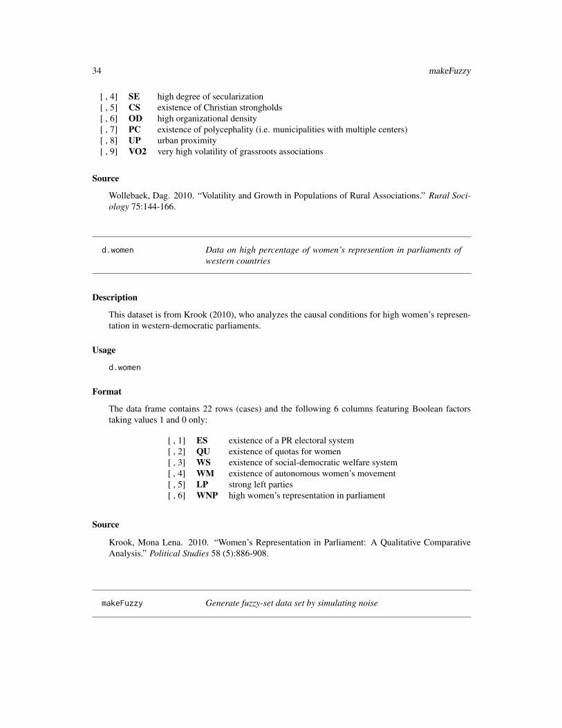
Description

This dataset is from Krook (2010), who analyzes the causal conditions for high women’s represen-tation in western-democratic parliaments.

Usage

d.women

Format


[ , 1] ES existence of a PR electoral system[ , 2] QU existence of quotas for women[ , 3] WS existence of social-democratic welfare system[ , 4] WM existence of autonomous women’s movement[ , 5] LP strong left parties[ , 6] WNP high women’s representation in parliament

Source

Krook, Mona Lena. 2010. “Women’s Representation in Parliament: A Qualitative ComparativeAnalysis.” Political Studies 58 (5):886-908.

makeFuzzy Generate fuzzy-set data set by simulating noise

makeFuzzy 35

Description

Generates fuzzy-set data by simulating the addition of random noise from the uncontrolled causalbackground to a data frame featuring Boolean factors only.

Usage

makeFuzzy(x, fuzzvalues = c(0, 0.05, 0.1), ...)

Arguments

x A data frame featuring Boolean factors with values 1 and 0 only.

fuzzvalues Values to be added to the 0’s and subtracted from the 1’s.

... Additional arguments are passed to truthTab.

Details

In combination with allCombs and selectCases, makeFuzzy is useful for simulating noisy data,which are needed for inverse search trials that assess the correctness of models output by cna.makeFuzzy transforms a data frame consisting of binary factors into a fuzzy-set truthTab by addingvalues selected at random from the argument fuzzvalues to the 0’s and subtracting them from the1’s in the data frame. This transformation simulates the introduction of background noise into thedata. selectCases can subsequently be applied to draw those fuzzy-set configurations from theresulting data that are compatible with a given data generating causal structure.

Value

A truthTab of type "fs".

See Also

selectCases, allCombs, truthTab, cna, tt2df, condition

Examples

# Fuzzify a binary 6x3 matrix with default fuzzvalues.X <- matrix(sample(0:1, 18, replace = TRUE), 6)makeFuzzy(X)

# ... and with customized fuzzvalues.makeFuzzy(X, fuzzvalues = 0:5/10)makeFuzzy(X, fuzzvalues = seq(0, 0.45, 0.01))

# Generate all configurations of 5 fuzzy-set factors that are compatible with the causal# structure A*b + C*D <-> E, such that con = .8 and cov = .8.dat1 <- allCombs(c(2, 2, 2, 2, 2)) - 1dat2 <- makeFuzzy(dat1, fuzzvalues = seq(0, 0.45, 0.01))(dat3 <- selectCases1("A*b + C*D <-> E", con = .8, cov = .8, dat2))condition("A*b + C*D <-> E", dat3)

# First, generate all configurations of 5 dichotomous factors that are compatible with

36 minimalizeCsf

# the causal chain (A*b + a*B <-> C)*(C*d + c*D <-> E) and, second, introduce background# noise.dat1 <- allCombs(c(2, 2, 2, 2, 2)) - 1dat2 <- selectCases("(A*b + a*B <-> C)*(C*d + c*D <-> E)", dat1)(dat3 <- makeFuzzy(tt2df(dat2), fuzzvalues = seq(0, 0.45, 0.01)))condition("(A*b + a*B <-> C)*(C*d + c*D <-> E)", dat3)

# Inverse search for the data generating causal structure A*b + a*B + C*D <-> E from# fuzzy-set data with non-perfect consistency and coverage scores.dat1 <- allCombs(c(2, 2, 2, 2, 2)) - 1set.seed(5)dat2 <- makeFuzzy(dat1, fuzzvalues = 0:4/10)dat3 <- selectCases1("A*b + a*B + C*D <-> E", con = .8, cov = .8, dat2)fscna(dat3, ordering = list("E"), strict = TRUE, con = .8, cov = .8)

minimalizeCsf Reduce csf by eliminating redundant parts

Description

minimalizeCsf reduces csf by recursively testing their component asf for redundancy and elimi-nating the redundant ones.

Usage

minimalizeCsf(x, ...)

## Default S3 method:minimalizeCsf(x, data, verbose = FALSE, ...)## S3 method for class 'cna'minimalizeCsf(x, n = 20, verbose = FALSE, ...)## S3 method for class 'minimalizeCsf'print(x, subset = 1:5, ...)

Arguments

x In the default method, x is a character vector specifying csf. The cna methoduses the strings representing the csf contained in an output object of cna.

data A truthTab, data.frame or matrix with the data.

verbose Logical, if TRUE additional messages on the number of csf that are found to bereducible are printed.

n Minimal number of csf to use.

subset Integer vector specifying the numbers of csf to be displayed.

... Further arguments passed to the methods.

minimalizeCsf 37

Details

The core criterion that Boolean dependency structures must satisfy in order to be causally inter-pretable is redundancy-freeness. In atomic solution formulas (asf), both sufficient and necessaryconditions are completely free of redundant elements. However, when asf are conjunctively com-bined to complex solution formulas (csf), new redundancies may arise. A csf may contain redundantparts. To illustrate, assume that a csf is composed of three asf: asf1 * asf2 * asf3. It can happen thatasf1 * asf2 * asf3 is logically equivalent to a proper part of itself, say, to asf1 * asf2. In that case,asf3 is redundant in asf1 * asf2 * asf3 and must not be causally interpreted.

minimalizeCsf recursively tests the asf contained in a csf for redundancy and eliminates theredundant ones. More specifically, it takes a character vector x specifying csf as input and builds allredundancy-free csf that can be inferred from x. The function is especially useful in combinationwith cna, which builds csf by conjunctively concatenating asf. One of the cna solution attributes,which is accessed via details = TRUE or details = "r", is called "redundant". If a csf output bycna has the attribute redundant = TRUE, that csf has at least one redundant part. The cna function,however, does not identify those redundant parts. For this purpose, the cna object must be passedon to minimalizeCsf.

Value

minimalizeCsf returns an object of class "minimalizeCsf", essentially a data.frame.

Contributors

Falk, Christoph: identification of the problem of structural redundancies

See Also

csf, cna.

Examples

myData <- allCombs(rep(2, 6))-1minimalizeCsf("(f + a*D <-> C)*(C + A*B <-> D)*(c + a*E <-> F)",

myData)minimalizeCsf("(f + a*D <-> C)*(C + A*B <-> D)*(c + a*E <-> F)",

myData, verbose = TRUE) # Same result, but with some messages.

# cna method.dat1 <- selectCases("(C + A*B <-> D)*(c + a*E <-> F)", myData)ana1 <- cna(dat1, details = c("r"))csf(ana1)# The attribute "redundant" taking the value TRUE in ana1 shows that this csf contains# at least one redundant element. Only the application of minimalizeCsf() identifies# the redundant element.minimalizeCsf(ana1)

# Real data entailing a large number of csf with many redundancies.tt.js <- fstt(d.jobsecurity)cna.js <- cna(tt.js, con = .8, cov = .8)minim100 <- minimalizeCsf(cna.js, n = 100) # may take a couple of seconds...

38 selectCases

minim100 # By default the first 5 solutions are displayed.

# With mv data.tt.pban <- mvtt(d.pban)cna.pban <- cna(tt.pban, con = .75, cov = .75)csf.pban <- csf(cna.pban, 100)sol.pban <- csf.pban$condition

minim.pban <- minimalizeCsf(sol.pban, tt.pban)minim.pban

# Alternatively, a more direct replication of the above using the method of# minimalizeCsf for class cna.minim.pban <- minimalizeCsf(cna.pban, n = 100)print(minim.pban, 1:50) # print the first 50 redundancy-free csf

selectCases Select the cases/configurations that are compatible with a data gener-ating causal structure

Description

Selects the cases/configurations that are compatible with a function, in particular (but not exclu-sively), a data generating causal structure, from a data frame or truth table.selectCases1 allows to set consistency (con) and coverage (cov) thresholds. It then selectscases/configurations that are compatible with the data generating structure to degrees con and cov.

Usage

selectCases(cond, x, type, cutoff = 0.5,rm.dup.factors = FALSE, rm.const.factors = FALSE)

selectCases1(cond, x, type, con = 1, cov = 1,rm.dup.factors = FALSE, rm.const.factors = FALSE)

Arguments

cond A character string specifying the Boolean function for which compatible casesare to be selected.

x A data frame or truthTab.type A character vector specifying the type of x: "cs" (crisp-set), "mv" (multi-value),

or "fs" (fuzzy-set). Defaults to the type of x, if x is a truthTab or to "cs"otherwise.

cutoff Cutoff value in case of "fs" data.rm.dup.factors Logical; if TRUE, all but the first of a set of factors with identical value distribu-

tions are eliminated.rm.const.factors

Logical; if TRUE, constant factors are eliminated.con, cov Numeric scalars between 0 and 1 to set the minimum consistency and coverage

thresholds.

selectCases 39

Details

In combination with allCombs and makeFuzzy, selectCases is useful for simulating data, whichare needed for inverse search trials that assess the correctness of models output by cna.

selectCases draws those cases/configurations from a given data frame or truthTab that are com-patible with a data generating causal structure (or any other Boolean or set-theoretic function),which is given to selectCases as a character string cond. cond can be a condition of any of thethree types of conditions, boolean, atomic or complex (see condition). To illustrate, if the datagenerating structure is "A + B <-> C", then a case featuring A=1, B=0, and C=1 is selected byselectCases, whereas a case featuring A=1, B=0, and C=0 is not (because according to the datagenerating structure, A=1 must be associated with C=1, which is violated in the latter case). Thetype of the data frame is specified by the argument type taking "cs" (crisp-set), "mv" (multi-value),and "fs" (fuzzy-set) as values.

selectCases1 allows for providing consistency (con) and coverage (cov) thresholds, such thatsome cases that are incompatible with cond are also drawn, as long as con and cov remain satisfied.The solution is identified by an algorithm aiming at finding a subset of maximal size meeting thecon and cov requirements. In contrast to selectCases, selectCases1 only accepts a condition oftype atomic as its cond argument, i.e. an atomic solution formula. Data drawn by selectCases1can only be modeled with consistency = con and coverage = cov.

Value

A truthTab.

See Also

allCombs, makeFuzzy, truthTab, condition, cna, d.jobsecurity

Examples

# Generate all configurations of 5 dichotomous factors that are compatible with the causal# chain (A*b + a*B <-> C) * (C*d + c*D <-> E).dat1 <- allCombs(c(2, 2, 2, 2, 2)) - 1(dat2 <- selectCases("(A*b + a*B <-> C) * (C*d + c*D <-> E)", dat1))condition("(A*b + a*B <-> C) * (C*d + c*D <-> E)", dat2)

# Generate all configurations of 5 multi-value factors that are compatible with the causal# chain (A=2*B=1 + A=3*B=3 <-> C=1) * (C=1*D=2 + C=4*D=4 <-> E=3).dat1 <- allCombs(c(3, 3, 4, 4, 3))(dat2 <- selectCases("(A=2*B=1 + A=3*B=3 <-> C=1) * (C=1*D=2 + C=4*D=4 <-> E=3)", dat1,

type = "mv"))condition("(A=2*B=1 + A=3*B=3 <-> C=1) * (C=1*D=2 + C=4*D=4 <-> E=3)", dat2)

# Generate all configurations of 5 fuzzy-set factors that are compatible with the causal# structure A*b + C*D <-> E, such that con = .8 and cov = .8.dat1 <- allCombs(c(2, 2, 2, 2, 2)) - 1dat2 <- makeFuzzy(dat1, fuzzvalues = seq(0, 0.45, 0.01))(dat3 <- selectCases1("A*b + C*D <-> E", con = .8, cov = .8, dat2))condition("A*b + C*D <-> E", dat3)

# Inverse search for the data generating causal structure A*b + a*B + C*D <-> E from

40 some

# fuzzy-set data with non-perfect consistency and coverage scores.dat1 <- allCombs(c(2, 2, 2, 2, 2)) - 1set.seed(9)dat2 <- makeFuzzy(dat1, fuzzvalues = 0:4/10)dat3 <- selectCases1("A*b + a*B + C*D <-> E", con = .8, cov = .8, dat2)fscna(dat3, ordering = list("E"), strict = TRUE, con = .8, cov = .8)

# Draw cases satisfying specific conditions from real-life fuzzy-set data.tt.js <- fstt(d.jobsecurity)selectCases("S -> C", tt.js) # Cases with higher membership scores in C than in S.selectCases("S -> C", d.jobsecurity, type = "fs") # Same.selectCases("S <-> C", tt.js) # Cases with identical membership scores in C and in S.selectCases1("S -> C", con = .8, cov = .8, tt.js) # selectCases1 makes no distinction

# between "->" and "<->".condition("S -> C", selectCases1("S -> C", con = .8, cov = .8, tt.js))

# selectCases not only draws cases compatible with Boolean causal models. Any Boolean or# set-theoretic function can be given as cond.selectCases("C > B", allCombs(2:4), type = "mv")selectCases("C=2 | B!=3", allCombs(2:4), type = "mv")selectCases("A=1 * !(C=2 + B!=3)", allCombs(2:4), type = "mv")

some Randomly select configurations from a data frame or truthTab

Description

Randomly select configurations from a data frame or truthTab with or without replacement.

Usage

some(x, ...)

## S3 method for class 'data.frame'some(x, n = 10, replace = TRUE, ...)## S3 method for class 'truthTab'some(x, n = 10, replace = TRUE, ...)

Arguments

x A truthTab

n Sample size

replace Logical; if TRUE, configurations are sampled with replacement.

... Not used

some 41

Details

some randomly samples configurations from x. Such samples can, for instance, be used to simulatedata fragmentation (limited diversity), i.e. the failure to observe/measure all configurations that arecompatible with a data generating causal structure. They can also be used to simulate large-N datafeaturing multiple cases instantiating each configuration.

Value

A data frame or truthTab.

Note

The some generic function and the method for data frames are adopted from the car package. Inparticular, our data.frame-method has an additional argument replace, which is TRUE by default.It will by default not apply the same sampling scheme as the method in car.

References

Krook, Mona Lena. 2010. “Women’s Representation in Parliament: A Qualitative ComparativeAnalysis.” Political Studies 58(5):886-908.

See Also

truthTab, selectCases, allCombs, makeFuzzy, cna, d.women

Examples

# Randomly sample configurations from the dataset analyzed by Krook (2010).tt.women <- truthTab(d.women)some(tt.women, 20)some(tt.women, 5, replace = FALSE)some(tt.women, 5, replace = TRUE)

# Simulate limited diversity in data generated by the causal structure# A=2*B=1 + C=3*D=4 <-> E=3.dat1 <- allCombs(c(3, 3, 4, 4, 3))dat2 <- selectCases("A=2*B=1 + C=3*D=4 <-> E=3", dat1, type = "mv")(dat3 <- some(dat2, 150, replace = TRUE))mvcna(dat3)

# Simulate large-N fuzzy-set data generated by the common-cause structure# (A*b*C + B*c <-> D) * (A*B + a*C <-> E).dat1 <- allCombs(c(2, 2, 2, 2, 2)) - 1dat2 <- selectCases("(A*b*C + B*c <-> D) * (A*B + a*C <-> E)", dat1)dat3 <- some(dat2, 250, replace = TRUE)dat4 <- makeFuzzy(tt2df(dat3), fuzzvalues = seq(0, 0.45, 0.01))fscna(dat4, ordering = list(c("D", "E")), strict = TRUE, con = .8, cov = .8)

42 truthTab

truthTab Assemble cases with identical configurations in a truth table

Description

This function assembles cases with identical configurations from a crisp-set (cs), multi-value (mv),or fuzzy-set (fs) data frame in a table called a truth table (which is a very different type of objectfor CNA than for the related method of QCA).

Usage

truthTab(x, type = c("cs", "mv", "fs"), frequency = NULL,case.cutoff = 0, rm.dup.factors = TRUE, rm.const.factors = TRUE,.cases = NULL, verbose = TRUE)

cstt(...)mvtt(...)fstt(...)

## S3 method for class 'truthTab'print(x, show.cases = NULL, ...)

Arguments

x A data frame or matrix.

type A character vector specifying the type of x: "cs" (crisp-set), "mv" (multi-value),or "fs" (fuzzy-set).

frequency Numeric vector of length nrow(x). All elements must be non-negative.

case.cutoff Minimum number of occurrences (cases) of a configuration in x. Configurationswith fewer than case.cutoff occurrences (cases) are not included in the truthtable.

rm.dup.factors Logical; if TRUE, all but the first of a set of factors with identical values in x areeliminated.

rm.const.factors

Logical; if TRUE, factors with constant values in x are eliminated.

.cases Set case labels (row names): optional character vector of length nrow(x).

verbose Logical; if TRUE, some informative messages on the truth table are printed.

show.cases Logical; if TRUE, the attribute “cases” is printed.

... In cstt, mvtt, fstt: any formal argument of truthTab except type. Inprint.truthTab: arguments passed to print.data.frame.

truthTab 43

Details

The first input x of the truthTab function is a data frame. To ensure that no misinterpretationsof issued asf and csf can occur, users are advised to use only upper case letters as factor (column)names. Column names may contain numbers, but the first sign in a column name must be a letter.Only ASCII signs should be used for column and row names.

The truthTab function merges multiple rows of x featuring the same configuration into one row,such that each row of the resulting table, which is called a truth table, corresponds to one determi-nate configuration of the factors in x. The number of occurrences (cases) and an enumeration ofthe cases are saved as attributes “n” and “cases”, respectively. The attribute “n” is always printed inthe output of truthTab, the attribute “cases” is printed if the argument show.cases is TRUE in theprint method.

The argument type specifies the type of data. "cs" stands for crisp-set data featuring factors thatonly take values 1 and 0; "mv" stands for multi-value data with factors that can take any non-negative integers as values; "fs" stands for fuzzy-set data comprising factors taking real valuesfrom the interval [0,1], which are interpreted as membership scores in fuzzy sets. To abbreviate thespecification of the data type using the type argument, the functions cstt(x, ...), mvtt(x, ...),and fstt(x, ...) are available as shorthands for truthTab(x, type = "cs", ...),truthTab(x, type = "mv", ...), and truthTab(x, type = "fs", ...), respectively.

Instead of multiply listing identical configurations in x, the frequency argument can be used toindicate the frequency of each configuration in the data frame. frequency takes a numeric vectorof length nrow(x) as value. For instance, truthTab(x, frequency = c(3,4,2,3)) determinesthat the first configuration in x is featured in 3 cases, the second in 4, the third in 2, and the fourthin 3 cases.

The case.cutoff argument is used to determine that configurations are only included in the truthtable if they are instantiated at least as many times in x as the number assigned to case.cutoff.Or differently, configurations that are instantiated less than the number given to case.cutoff areexcluded from the truth table. For instance, truthTab(x, case.cutoff = 3) entails that config-urations with less than 3 cases are excluded.

rm.dup.factors and rm.const.factors allow for determining whether all but the first of a set ofduplicated factors (i.e. factors with identical value distributions in x) are eliminated and whetherconstant factors (i.e. factors with constant values in all cases (rows) in x) are eliminated. From theperspective of configurational causal modeling, factors with constant values in all cases can neitherbe modeled as causes nor as outcomes; therefore, they can be removed prior to the analysis. Factorswith identical value distributions cannot be distinguished configurationally, meaning they are oneand the same factor as far as configurational causal modeling is concerned. Therefore, only onefactor of a set of duplicated factors is standardly retained by truthTab.

.cases can be used to set case labels (row names). It is a character vector of length nrow(x).

The row.names argument of the print function determines whether the case labels of x are printedor not. By default, row.names is TRUE unless the (comma-separated) list of the cases exceeds 20characters in one row at least.

Value

A “truthTab”, i.e. a data.frame with additional attributes “type”, “n” and “cases”.

44 truthTab

Note

For those users of cna that are familiar with Qualitative Comparative Analysis (QCA), it must beemphasized that a truth table is a very different type of object in the context of CNA than it isin the context of QCA. While a QCA truth table is a list indicating whether a minterm (i.e. aconfiguration of all exogenous factors) is sufficient for the outcome or not, a CNA truth table issimply an integrated representation of the input data that lists all configurations in the data exactlyonce. A CNA truth table does not express any relations of sufficiency whatsoever.

References

Aleman, Jose. 2009. “The Politics of Tripartite Cooperation in New Democracies: A Multi-levelAnalysis.” International Political Science Review 30 (2):141-162.

Greckhamer, Thomas, Vilmos F. Misangyi, Heather Elms, and Rodney Lacey. 2008. “Using Quali-tative Comparative Analysis in Strategic Management Research: An Examination of Combinationsof Industry, Corporate, and Business-Unit Effects.” Organizational Research Methods 11 (4):695-726.

Thiem, Alrik. 2018. “QCApro: Advanced Functionality for Performing and Evaluating QualitativeComparative Analysis.” R Package Version 1.1-2. URL: http://www.alrik-thiem.net/software/.

See Also

cna, condition, allCombs, d.performance, d.pacts

Examples

# Manual input of cs data# -----------------------dat1 <- data.frame(

A = c(1,1,1,1,1,1,1,1,1,1,1,1,1,1,1,1,0,0,0,0,0,0,0,0,0,0,0,0,0,0,0,0,0,0,0,0),B = c(1,1,1,1,1,1,1,1,0,0,0,0,0,0,0,0,1,1,1,1,1,1,1,1,1,1,1,1,1,1,0,0,0,0,0,0),C = c(1,1,1,1,1,1,1,1,1,1,1,1,1,1,1,1,1,1,1,1,1,1,1,1,1,1,1,1,1,1,0,0,0,0,0,0),D = c(1,1,1,1,0,0,0,0,1,1,1,0,0,0,0,0,1,1,1,1,1,1,1,1,1,1,1,0,0,0,1,1,1,0,0,0),E = c(1,1,1,1,1,1,1,0,1,1,1,1,1,1,1,0,1,1,1,1,1,1,1,1,1,1,0,1,1,1,1,1,1,0,0,0)

)

# Default return of the truthTab function.truthTab(dat1)

# Recovering the cases featuring each configuration by means of the print function.print(truthTab(dat1), show.cases = TRUE)

# The same truth table as before can be generated by using the frequency argument while# listing each configuration only once.dat1 <- data.frame(

A = c(1,1,1,1,1,1,0,0,0,0,0),B = c(1,1,1,0,0,0,1,1,1,0,0),C = c(1,1,1,1,1,1,1,1,1,0,0),D = c(1,0,0,1,0,0,1,1,0,1,0),E = c(1,1,0,1,1,0,1,0,1,1,0)

)

truthTab 45

truthTab(dat1, frequency = c(4,3,1,3,4,1,10,1,3,3,3))

# Set (random) case labels.print(truthTab(dat1, .cases = sample(letters, nrow(dat1), replace = FALSE)),

show.cases = TRUE)

# Truth tables generated by truthTab can be input into the cna function.dat1.tt <- truthTab(dat1, frequency = c(4,3,1,3,4,1,4,1,3,3,3))cna(dat1.tt, con = .85, details = TRUE)

# By means of the case.cutoff argument configurations with less than 2 cases can# be excluded (which yields perfect consistency and coverage scores for dat1).dat1.tt <- truthTab(dat1, frequency = c(4,3,1,3,4,1,4,1,3,3,3), case.cutoff = 2)cna(dat1.tt, details = TRUE)

# Simulating multi-value data with biased samples (exponential distribution)# --------------------------------------------------------------------------dat1 <- allCombs(c(3,3,3,3,3))set.seed(32)m <- nrow(dat1)wei <- rexp(m)dat2 <- dat1[sample(nrow(dat1), 100, replace = TRUE, prob = wei),]truthTab(dat2, type = "mv") # 100 cases with 46 configurations instantiated only once.dat3 <- mvtt(dat2, case.cutoff = 2) # removing the single instances.mvcna(dat3)

# Duplicated factors are not eliminated, constant factors are not eliminated.dat4 <- selectCases("(A=1+A=2+A=3 <-> C=2)*(B=3<->D=3)*(B=2<->D=2)*(A=2 + B=1 <-> E=2)",

dat1, type = "mv")mvtt(dat4, rm.dup.factors = FALSE, rm.const.factors = FALSE)

# truthTab with fuzzy-set data from Aleman (2009)# -----------------------------------------------# Include all cases.tt.pacts <- fstt(d.pacts)fscna(tt.pacts, con = .93, cov = .86, details = TRUE)

# Only include configurations with at least 3 cases.tt.pacts2 <- fstt(d.pacts, case.cutoff = 3)fscna(tt.pacts2, con = .93, cov = .86, details = TRUE)

# Large-N data with crisp sets from Greckhamer et al. (2008)#-----------------------------------------------------------truthTab(d.performance[1:8], frequency = d.performance$frequency)

# Eliminate configurations with less than 5 cases.truthTab(d.performance[1:8], frequency = d.performance$frequency, case.cutoff = 5)

# Various large-N CNAs of d.performance with varying case cut-offs.cna(truthTab(d.performance[1:8], frequency = d.performance$frequency, case.cutoff = 4),

ordering = list("SP"), con = .75, cov = .6)cna(truthTab(d.performance[1:8], frequency = d.performance$frequency, case.cutoff = 5),

ordering = list("SP"), con = .75, cov = .6)

46 tt2df

cna(truthTab(d.performance[1:8], frequency = d.performance$frequency, case.cutoff = 10),ordering = list("SP"), con = .75, cov = .6)

print(cna(truthTab(d.performance[1:8], frequency = d.performance$frequency, case.cutoff = 15),ordering = list("SP"), con = .75, cov = .6, what = "a"), nsolutions = "all")

tt2df Transform a truth table into a data frame

Description

Transform a truth table into a data frame. This is the converse function of truthTab.

Usage

tt2df(tt)

Arguments

tt A truthTab

Details

Rows in the truthTab corresponding to several cases are rendered as multiple rows in the resultingdata frame.

Value

A data frame.

See Also

truthTab

Examples

tt.educate <- truthTab(d.educate[1:2])tt.educatett2df(tt.educate)

dat1 <- some(truthTab(allCombs(c(2, 2, 2, 2, 2)) - 1), n = 200, replace = TRUE)dat2 <- selectCases("(A*b + a*B <-> C)*(C*d + c*D <-> E)", dat1)dat2tt2df(dat2)

dat3 <- data.frame(A = c(1,1,1,1,1,1,0,0,0,0,0),B = c(1,1,1,0,0,0,1,1,1,0,0),C = c(1,1,1,1,1,1,1,1,1,0,0),D = c(1,0,0,1,0,0,1,1,0,1,0),

tt2df 47

E = c(1,1,0,1,1,0,1,0,1,1,0))

tt.dat3 <- truthTab(dat3, frequency = c(4,3,5,7,4,6,10,2,4,3,12))tt2df(tt.dat3)

Index

∗Topic datasetsd.autonomy, 27d.educate, 28d.irrigate, 29d.jobsecurity, 30d.minaret, 30d.pacts, 31d.pban, 32d.performance, 32d.volatile, 33d.women, 34

∗Topic packagecna-package, 2

allCombs, 4, 18, 35, 39, 41, 44as.condTbl (condTbl), 24asf (condTbl), 24

cna, 5, 18–20, 22, 24–26, 35, 37, 39, 41, 44cna-package, 2coherence, 9, 12, 17condition, 12, 18, 19, 24–26, 35, 39, 44condTbl, 12, 18, 22, 24cscna (cna), 5cscond (condition), 19csf, 37csf (condTbl), 24cstt (truthTab), 42

d.autonomy, 12, 27d.educate, 12, 28d.irrigate, 22, 26, 29d.jobsecurity, 30, 39d.minaret, 30d.pacts, 31, 44d.pban, 12, 32d.performance, 32, 44d.volatile, 33d.women, 12, 34, 41

fscna (cna), 5

fscond (condition), 19fstt (truthTab), 42

group.by.outcome (condition), 19

makeFuzzy, 4, 12, 34, 39, 41minimalizeCsf, 10, 12, 26, 36msc (condTbl), 24mvcna (cna), 5mvcond (condition), 19mvtt (truthTab), 42

print.cna (cna), 5print.cond (condition), 19print.condList (condition), 19print.condTbl (condTbl), 24print.data.frame, 25, 42print.minimalizeCsf (minimalizeCsf), 36print.truthTab, 7, 20print.truthTab (truthTab), 42

selectCases, 4, 12, 18, 35, 38, 41selectCases1 (selectCases), 38some, 12, 40summary.condList (condition), 19

truthTab, 6, 7, 12, 19, 20, 22, 26, 35, 36, 39,41, 42, 46

tt2df, 35, 46

48

package ‘cna’ - r · package ‘cna ’ june 13, 2018 type ... ness, and a test for structural...

Documents