package ‘ecovirtual’ - the comprehensive r …...package ‘ecovirtual’ october 11, 2018 type...

Package ‘EcoVirtual’October 11, 2018

Type Package

Title Simulation of Ecological Models

Version 1.1

Date 2018-10-10

Author Alexandre Adalardo de Oliveira and Paulo Inacio Prado

<[email protected]>

Maintainer Alexandre Adalardo de Oliveira <[email protected]>

Description Computer simulations of classical ecological models as alearning resource.

Depends tcltk

License GPL (>= 2)

URL http//ecovirtual.ib.usp.br

LazyLoad yes

RoxygenNote 5.0.1

NeedsCompilation no

Repository CRAN

Date/Publication 2018-10-11 04:20:07 UTC

R topics documented:anima . . . . . . . . . . . . . . . . . . . . . . . . . . . . . . . . . . . . . . . . . . . . 2animaColExt . . . . . . . . . . . . . . . . . . . . . . . . . . . . . . . . . . . . . . . . 3archip . . . . . . . . . . . . . . . . . . . . . . . . . . . . . . . . . . . . . . . . . . . . 4bioGeoIsl . . . . . . . . . . . . . . . . . . . . . . . . . . . . . . . . . . . . . . . . . . 6comCompete . . . . . . . . . . . . . . . . . . . . . . . . . . . . . . . . . . . . . . . . 7compLV . . . . . . . . . . . . . . . . . . . . . . . . . . . . . . . . . . . . . . . . . . . 8dynPop . . . . . . . . . . . . . . . . . . . . . . . . . . . . . . . . . . . . . . . . . . . 9extGame . . . . . . . . . . . . . . . . . . . . . . . . . . . . . . . . . . . . . . . . . . . 12metaComp . . . . . . . . . . . . . . . . . . . . . . . . . . . . . . . . . . . . . . . . . . 13metaPop . . . . . . . . . . . . . . . . . . . . . . . . . . . . . . . . . . . . . . . . . . . 14randWalk . . . . . . . . . . . . . . . . . . . . . . . . . . . . . . . . . . . . . . . . . . 16

1

2 anima

regNicho . . . . . . . . . . . . . . . . . . . . . . . . . . . . . . . . . . . . . . . . . . 17rich . . . . . . . . . . . . . . . . . . . . . . . . . . . . . . . . . . . . . . . . . . . . . 19simHub . . . . . . . . . . . . . . . . . . . . . . . . . . . . . . . . . . . . . . . . . . . 19sucMatrix . . . . . . . . . . . . . . . . . . . . . . . . . . . . . . . . . . . . . . . . . . 21

Index 23

anima Internal EcoVirtual Graphics and Animations

Description

Internal functions for graphics and animations of the simulations results.

Usage

grColExt(E, I, P, area)

Arguments

E extinction rate

I colonization rate

P species available in mainland

area islands sizes

Details

The list below relates each function graphical and its primary functions:

animaCena - regNicho

animaGame - extGame

animaHub - simHub1, simHub2, simHub3

animaIsl - archip

animaMeta2 - metaPop, metaCi, metaEr, metaCiEr

animaMetaComp - metaComp

animaRandWalk - randWalk

grColExt - animaColExt, bioGeoIsl

grFim - metaPop, metaCi, metaEr, metaCiEr

Value

Show simulation in a graphic device.

Author(s)

Alexandre Adalardo de Oliveira <[email protected]>

animaColExt 3

See Also

http://ecovirtual.ib.usp.br

Examples

## Not run:grColExt(E = 0.5 , I = 0.5 , P = 100, area=1:10)

## End(Not run)

animaColExt Colonization and Extinction balance in the Island Biogeography Equi-librium model

Description

Simulate the balance between extinction and colonization rates given the equilibrium number ofspecies in a island, based on the Island Biogeography Equilibrium model.

Usage

animaColExt(min = 0.01, max = 1, cycles = 100, Ext = "crs",Col = "dcr")

Arguments

min between 0-1. The minimum value of the extinction and colonization rates.

max between 0-1. The maximum value of the extinction and colonization rates.

cycles number of cycles in the simulation.

Ext a string representing the extinction rate. This can be ’crs’ for an increasingextinction rate, ’fix’ for a fixed extinction rate in 0.5, or ’dcr’ for a decreasingextinction rate.

Col a string representing the colonization rate. This can be ’crs’ for an increasingcolonization rate, ’fix’ for a fixed colonization rate in 0.5, or ’dcr’ for a decreas-ing colonization rate.

Details

The number of species is the balance between extinction and colonization rates at the equilibrium.

Value

’animaColExt’ returns a graph of the extinction and colonization rates varying one or both rates inrelation with the number of species of an island.


4 archip

Author(s)


References

Gotelli, N.J. 2008. A primer of Ecology. 4th ed. Sinauer Associates, 291pp.

See Also

archip bioGeoIsl http://ecovirtual.ib.usp.br

Examples

## Not run:animaColExt(Ext='fix', Col="fix")

## End(Not run)

archip Species Colonization and Species-Area Relationship in Archipelagos

Description

Simulate species colonization from mainland to islands with different sizes.

Usage

archip(n.isl, ar.min, ar.max, S, seed.rain, abund, tmax = 100, anima = TRUE)

Arguments

n.isl numeric, number of islands.

ar.min numeric, area of the smallest island.

ar.max numeric, area of the biggest island.

S numeric, number of species (species richness from mainland).

seed.rain numeric, seed rain. Number of seeds colonizing islands on each time.

abund numeric, abundance of each species in the seed rain.

tmax numeric, maximum time for the simulations.

anima logical; if TRUE, show simulation frames.


archip 5

Details

The mainland has richness (S) and the evenness can be controled argument abund. The ’abund’argument can be one of these 3 options:

1. a vector with the same length of the species richness, meaning the proportion of each speciespopulation;

2. a single value more than 1 representing equal abundance of each species (maximum evenness);

3. a single value between 0 and 1, meaning the model of geometric species rank-abundancedistribution. The model is: abund*(1-abund)*((1:S)-1), where S is the number of species.

Value

’archip’ returns 3 graphics:

• The species-area relationship: number of species x island area at the end of the simulation. Italso returns the coefficients c and z from species-area relationship S = cAz .

• Colonization rate curves: colonization (number of species per cycle) x number of species foreach island.

• Passive colonization: number of species x time for each island.’archip’ also returns an invisible array with the simulation results.

Author(s)


References


See Also

animaColExt, bioGeoIsl, http://ecovirtual.ib.usp.br

Examples

## Not run:archip(n.isl=10,ar.min=10, ar.max=100, S=1000, seed.rain=100, abund=10, tmax=100, anima=TRUE)

archip(n.isl=10,ar.min=10, ar.max=100, S=1000, seed.rain=100, abund=0.5, tmax=100, anima=TRUE)

## End(Not run)


6 bioGeoIsl

bioGeoIsl Island Biogeographical Model

Description

Simulates island biogeographical models, with rates of colonization and extinction for islands ofdifferent sizes and distances to the mainland.

Usage

bioGeoIsl(area, dist, P, weight.A = 0.5, a.e = 1, b.e = -0.01, c.i = 1,d.i = -0.01, e.i = 0, f.i = 0.01, g.e = 0, h.e = 0.01)

Arguments

area a vector with the sizes of the island areas. It must have the same length as ’dist’

dist a vector with the distances of the islands to the mainland. It must have the samelength as ’areas’

P the number of species in the mainland (species richness of the pool).

weight.A ratio between the area and distance effects. Should be a number between 0 to1. When the ration is 1 the extinction is only affected by size and colonizationonly by distance. The default ratio is 0.5, meaning that distance and size equallyinfluence colonization and extinction.

a.e basal extiction coefficient for area.

b.e extinction/area coefficient.

c.i basal colonization coefficient for distance.

d.i numeric, colonization/distance coefficient.

e.i basal colonization coefficient for area.

f.i colonization/area coefficient.

g.e basal extinction coefficient for distance.

h.e extinction/distance coefficient.

Value

’bioGeoIsl’ returns a graph with the rates of colonization and extinction in relation with the speciesrichness for each island.

’bioGeoIsl’ also returns a invisible data frame with the values for area, distance and species richness(S) for each island.

Author(s)


comCompete 7

References


See Also

animaColExt archip, http://ecovirtual.ib.usp.br

Examples

## Not run:bioGeoIsl(area=c(5,10,50,80), dist=c(10,100,100,10), P=100, weight.A=.5, a=1,b=-0.01, c=1, d=-0.01, e=0, f=.01, g=0, h=.01)

## End(Not run)

comCompete Multispecies competition-colonization tradeoff

Description

Simulates the trade-off between colonization and competition abilities in a multispecies system.

Usage

comCompete(rw, cl, S, fi, fsp1, pe, fr = 0, int = 0, tmax)

Arguments

rw number of rows for the simulated landscape.

cl number of columns for the simulated landscape.

S number of species.

fi initial fraction of patchs occupied

fsp1 superior competitor abundance.

pe mortality rate.

fr disturbance frequency.

int disturbance intensity.

tmax maximum simulation time.

Details

In the system, the competitive abilities are inversely proportional to the colonization abilities.

The number of patches in the simulated landscape is defined by rw*cl.


8 compLV

Value

’comCompete’ returns a graph with the proportion of patches occupied in time by each species andthe trade-off scale, the superior competitor in one side and the superior colonizator in the other.

Author(s)


References

Tilman. R. 1994. Competition and biodiversity in spatially structured habitats. Ecology,75:2-16.

Stevens, M.H.H. 2009. A primer in ecology with R. New York, Springer.

See Also

metaComp, http://ecovirtual.ib.usp.br

Examples

## Not run:comCompete(tmax=1000, rw=100, cl=100, S=10, fi=1, fsp1=0.20, pe=0.01, fr=0, int=0)

## End(Not run)

compLV Lotka-Volterra Competition Model

Description

Simulate the Lotka-Volterra competition model for two populations.

Usage

compLV(n01, n02, tmax, r1, r2, k1, k2, alfa, beta)

Arguments

n01 initial population for the superior competitor species.n02 initial population for the inferior competitor species.tmax maximum simulation time.r1 intrinsic growth rate for the superior competitor species.r2 intrinsic growth rate for the inferior competitor species.k1 carrying capacity for the superior competitor species.k2 carrying capacity for the inferior competitor species.alfa alfa coefficient.beta beta coefficient


dynPop 9

Details

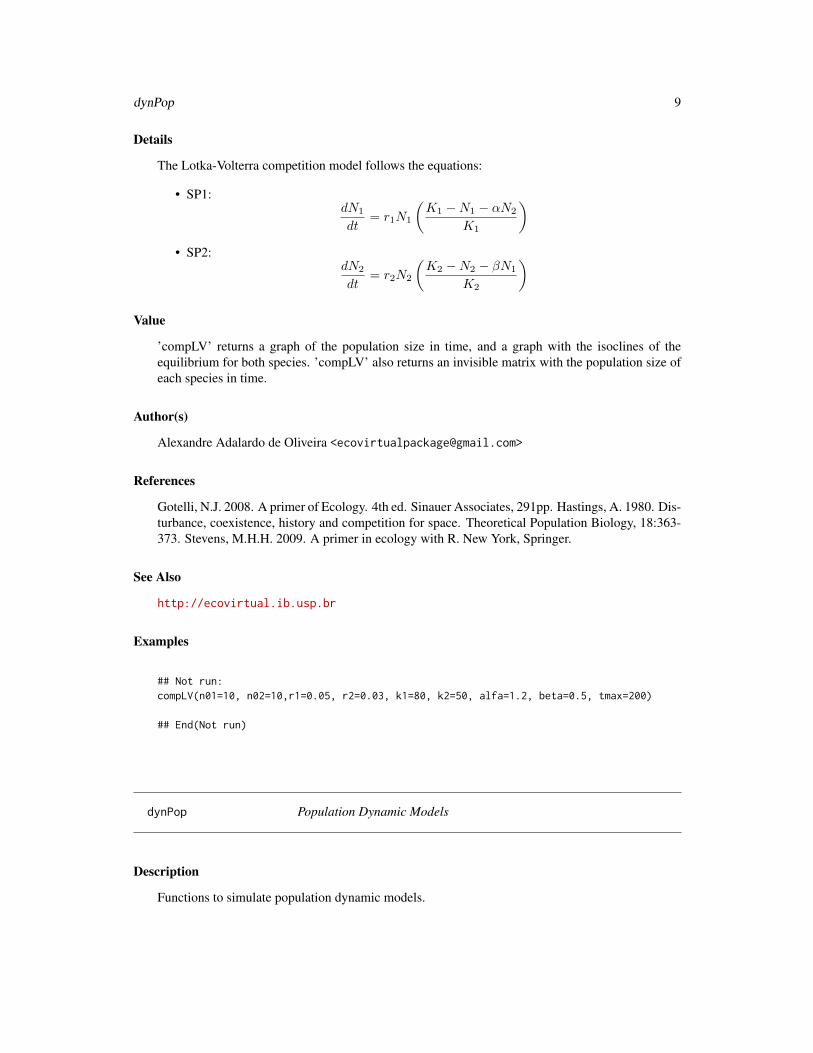
The Lotka-Volterra competition model follows the equations:

• SP1:dN1

dt= r1N1

(K1 −N1 − αN2

K1

)• SP2:

dN2

dt= r2N2

(K2 −N2 − βN1

K2

)

Value

’compLV’ returns a graph of the population size in time, and a graph with the isoclines of theequilibrium for both species. ’compLV’ also returns an invisible matrix with the population size ofeach species in time.

Author(s)


References

Gotelli, N.J. 2008. A primer of Ecology. 4th ed. Sinauer Associates, 291pp. Hastings, A. 1980. Dis-turbance, coexistence, history and competition for space. Theoretical Population Biology, 18:363-373. Stevens, M.H.H. 2009. A primer in ecology with R. New York, Springer.

See Also


Examples

## Not run:compLV(n01=10, n02=10,r1=0.05, r2=0.03, k1=80, k2=50, alfa=1.2, beta=0.5, tmax=200)

## End(Not run)

dynPop Population Dynamic Models

Description

Functions to simulate population dynamic models.


10 dynPop

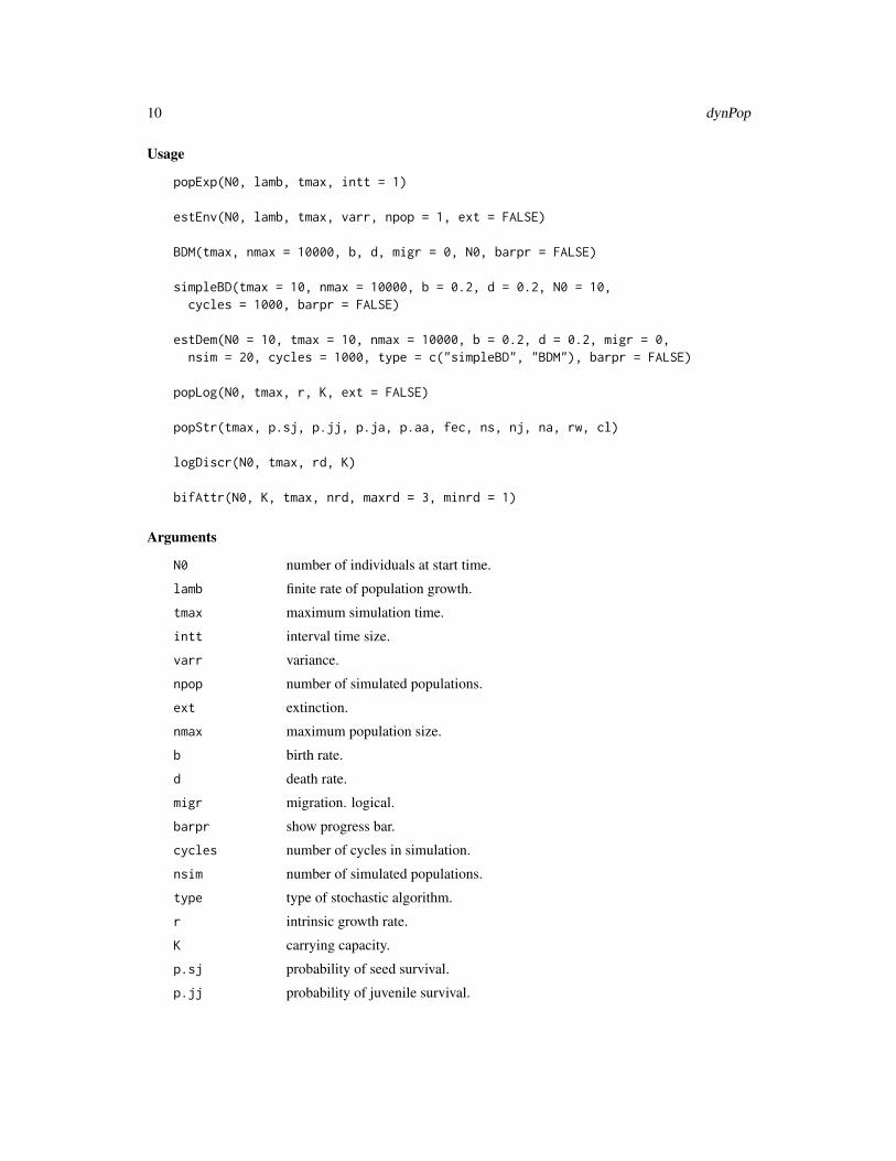
Usage

popExp(N0, lamb, tmax, intt = 1)

estEnv(N0, lamb, tmax, varr, npop = 1, ext = FALSE)

BDM(tmax, nmax = 10000, b, d, migr = 0, N0, barpr = FALSE)

simpleBD(tmax = 10, nmax = 10000, b = 0.2, d = 0.2, N0 = 10,cycles = 1000, barpr = FALSE)

estDem(N0 = 10, tmax = 10, nmax = 10000, b = 0.2, d = 0.2, migr = 0,nsim = 20, cycles = 1000, type = c("simpleBD", "BDM"), barpr = FALSE)

popLog(N0, tmax, r, K, ext = FALSE)

popStr(tmax, p.sj, p.jj, p.ja, p.aa, fec, ns, nj, na, rw, cl)

logDiscr(N0, tmax, rd, K)

bifAttr(N0, K, tmax, nrd, maxrd = 3, minrd = 1)

Arguments

N0 number of individuals at start time.

lamb finite rate of population growth.


intt interval time size.

varr variance.

npop number of simulated populations.

ext extinction.

nmax maximum population size.

b birth rate.

d death rate.

migr migration. logical.

barpr show progress bar.

cycles number of cycles in simulation.

nsim number of simulated populations.

type type of stochastic algorithm.

r intrinsic growth rate.

K carrying capacity.

p.sj probability of seed survival.

p.jj probability of juvenile survival.

dynPop 11

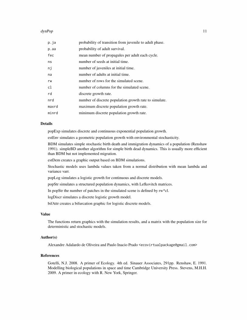
p.ja probability of transition from juvenile to adult phase.

p.aa probability of adult survival.

fec mean number of propagules per adult each cycle.

ns number of seeds at initial time.

nj number of juveniles at initial time.

na number of adults at initial time.

rw number of rows for the simulated scene.

cl number of columns for the simulated scene.

rd discrete growth rate.

nrd number of discrete population growth rate to simulate.

maxrd maximum discrete population growth rate.

minrd minimum discrete population growth rate.

Details

popExp simulates discrete and continuous exponential population growth.

estEnv simulates a geometric population growth with environmental stochasticity.

BDM simulates simple stochastic birth death and immigration dynamics of a population (Renshaw1991). simpleBD another algorithm for simple birth dead dynamics. This is usually more efficientthan BDM but not implemented migration.

estDem creates a graphic output based on BDM simulations.

Stochastic models uses lambda values taken from a normal distribution with mean lambda andvariance varr.

popLog simulates a logistic growth for continuous and discrete models.

popStr simulates a structured population dynamics, with Lefkovitch matrices.

In popStr the number of patches in the simulated scene is defined by rw*cl.

logDiscr simulates a discrete logistic growth model.

bifAttr creates a bifurcation graphic for logistic discrete models.

Value

The functions return graphics with the simulation results, and a matrix with the population size fordeterministic and stochastic models.

Author(s)

Alexandre Adalardo de Oliveira and Paulo Inacio Prado <[email protected]>

References

Gotelli, N.J. 2008. A primer of Ecology. 4th ed. Sinauer Associates, 291pp. Renshaw, E. 1991.Modelling biological populations in space and time Cambridge University Press. Stevens, M.H.H.2009. A primer in ecology with R. New York, Springer.

12 extGame

See Also

metaComp, http://ecovirtual.ib.usp.br

Examples

## Not run:popStr(p.sj=0.4, p.jj=0.6, p.ja=0.2, p.aa=0.9, fec=0.8, ns=100,nj=40,na=20, rw=30, cl=30, tmax=20)

## End(Not run)

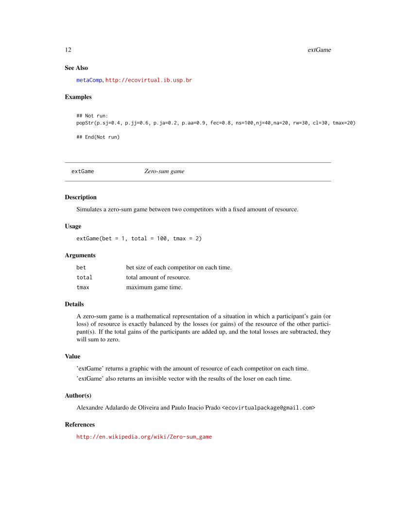
extGame Zero-sum game

Description

Simulates a zero-sum game between two competitors with a fixed amount of resource.

Usage

extGame(bet = 1, total = 100, tmax = 2)

Arguments

bet bet size of each competitor on each time.

total total amount of resource.

tmax maximum game time.

Details

A zero-sum game is a mathematical representation of a situation in which a participant’s gain (orloss) of resource is exactly balanced by the losses (or gains) of the resource of the other partici-pant(s). If the total gains of the participants are added up, and the total losses are subtracted, theywill sum to zero.

Value

’extGame’ returns a graphic with the amount of resource of each competitor on each time.

’extGame’ also returns an invisible vector with the results of the loser on each time.

Author(s)


References

http://en.wikipedia.org/wiki/Zero-sum_game


http://en.wikipedia.org/wiki/Zero-sum_game

metaComp 13

See Also

simHub, randWalk, http://ecovirtual.ib.usp.br

Examples

## Not run:extGame(bet=1,total=20)extGame(bet=1,total=100)

## End(Not run)

metaComp Metapopulation Competition Model

Description

Simulate a metapopulation dynamics with two competing species, a superior and an inferior com-petitor. Includes the possibility of habitat destruction in the model.

Usage

metaComp(tmax, rw, cl, f01, f02, i1, i2, pe, D = 0, anima = TRUE)

Arguments


rw number of rowns for the simulated landscape.


f01 initial fraction of patches occupied by the superior competitor.

f02 initial fraction of patches occupied by the inferior competitor.

i1 colonization coefficient for the superior competitor.

i2 colonization coefficient for the inferior competitor.

pe probability of extinction (equal for both species).

D proportion of habitat destroyed.

anima logical; if TRUE, show simulation frames.

Details

This function uses the metapopulationa model with internal colonization (see function metaCi inmetapopulation) for the superior competitor. The inferior competitor can only occupy emptypatches and is displaced by the superior competitor if it occupies the same patch.

The argument ’D’ inserts the influences of habitat destruction in the model.



14 metaPop

Value

’metaComp’ returns a graphic with the simulated landscapes and the results of the proportion ofpatch occupied by both species.

This function also return an invisible array with the simulation results.

Author(s)


References

Stevens, M.H.H. 2009. A primer in ecology with R. New York, Springer.

Gotelli, N.J. 1991. Metapopulation models: the rescue effect, the propagule rain, and the core-satellite hypothesis. The American Naturalist 138:768-776.

See Also

comCompete, http://ecovirtual.ib.usp.br

Examples

## Not run:metaComp(tmax=100,cl=20,rw=20,f01=0.1,f02=0.4,i1=0.4,i2=0.5,pe=0.25)metaComp(tmax=100,cl=20,rw=20,f01=0.1,f02=0.4,i1=0.4,i2=0.5,pe=0.25, D=0.1)

## End(Not run)

metaPop Metapopulation Models

Description

Simulate metapopulation dynamics with propagules seed rain, internal colonization and rescue ef-fect.

Usage

metaPop(cl, rw, f0, pi, pe, tmax, anima = TRUE)

metaCi(cl, rw, f0, ci, pe, tmax, anima = TRUE)

metaEr(cl, rw, f0, pi, ce, tmax, anima = TRUE)

metaCiEr(cl, rw, f0, ci, ce, tmax, anima = TRUE)


metaPop 15

Arguments



f0 initial proportion of occupied patches.

pi probability of colonization.

pe probability of extinction.


anima show animation frames.

ci colonization coefficient, represents the maximum probability of colonization(when f=1) and should be a number between 0 and 1.

ce coefficient of extinction, represents the maximum probability of extinction (whenf=0) and should be a number between 0 and 1.

Details

’metaPop’ is the seed rain metapopulation model, including only propagules seed rain from a ex-ternal pool (no extinction).

’metaCi’ is the Internal Colonization model, where number of propagules depends on number ofoccupied patches, there is no external pool.

’metaEr’ is the Rescue Effect model, where extinction probability is negatively associated withnumber of occupied patches.

’metaCiEr’ includes both effects: Rescue Effect and Internal Colonization.


Value

Metapopulation functions return graphics with the simulation results. These functions also returnan invisible array with the simulation data.

Author(s)


References

Gotelli, N.J. 1991. Metapopulation models: the rescue effect, the propagule rain, and the core-satellite hypothesis. The American Naturalist 138:768-776.


See Also



16 randWalk

Examples

## Not run:metaPop(cl=10,rw=10,f0=0.5,pi=0.3,pe=0.15, tmax=100)metaCi(cl=10,rw=10,f0=0.1,ci=1,pe=0.5, tmax=100)metaEr(cl=10, rw=10, f0=0.2, pi=0.2, ce=0.15, tmax=100)metaCiEr(cl=10, rw=10, f0=0.2, ci=0.2, ce=0.15, tmax=100)

## End(Not run)

randWalk Random Walk Simulations

Description

Simulates random walk models.

Usage

randWalk(S = 1, step = 1, tmax = 1e+05, x1max = 200, alleq = FALSE)

Arguments

S number of individuals.

step step size (number of steps on each time)


x1max maximum initial distance from absorption surface.

alleq logical; if TRUE, all initial distance are equal. if FALSE, initial distances foreach individual is a sample between 1 and maximum initial distance(x1max).

Details

Random walk is a stochastic process of a succession of random steps.

Zero is the absorption surface. When an individual simulation reaches zero, it means that the indi-vidual is dead.

See http://en.wikipedia.org/wiki/Random_walk.

Value

’randWalk’ returns a graphic with the simulated trajectories of each individual.

’randWalk’ also returns an invisible matrix with the distance from de edge for each individual oneach time.

Author(s)


http://en.wikipedia.org/wiki/Random_walk

regNicho 17

References


See Also

extGame, simHub, http://ecovirtual.ib.usp.br

Examples

## Not run:randWalk(S=100,step=2,tmax=2e5)randWalk(S=10,step=1,tmax=1e4, x1max=300, alleq=TRUE)

## End(Not run)

regNicho Successional Niche Model

Description

Simulates the process of niche succession by successional stages in a community with 2 species (asuperior and an inferior competitor), following the model of Pacala and Rees (1998).

Usage

regNicho(tmax, rw, cl, c1, c2, ec, dst, er, sc, mx, rs, anima = TRUE)

Arguments




c1 colonization rate for the late successional species (superior competitor).

c2 colonization rate for the early successional species (inferior competitor).

ec rate of competitive exclusion.

dst disturbance rate.

er inicial proportion of patches in early stage.

sc inicial proportion of patches in susceptible stage.

mx initial proportion of patches in mixed stage.

rs initial proportion of pathces in resistant stage.

anima show animation frames.



18 regNicho

Details

There are five possible states of this model:

• free - open, unoccupied space;

• early - occupied by only the early successional species;

• susceptible - occupied by only the late succesional species and susceptible to invasion by theearly succesional species;

• mixed - occupied by both species;

• resistant - occupied by only the late successional species.

The early successional species is the inferior competitor in the model, and the later successionalspecies is the superior competitor.


’dst’ is the proportion of patches in any stage that turns empty, it represents a disturbance in thelandscape.

’ec’ is the probability of succeptible and mixed stages turns resistant stage.

Value

’regNicho’ returns the simulation results of patch occupancy in time for each successional stage.

’regNicho’ also returns an invisible array with the simulation results per time.

Author(s)


References

Pacala, S & Rees, M. 1998. Models suggesting field experiments to test two hypotheses explainingsuccessional diversity. The American Naturalist 152(2): 729:737.

Stevens, MHH. 2009. A primer in ecology with R. New York, Springer.

See Also

comCompete, http://ecovirtual.ib.usp.br

Examples

## Not run:regNicho(tmax=50, rw=100, cl=100, c1=0.2, c2=0.8, ec=0.5, dst=0.04, er=0.08, sc=0.02, mx=0, rs=0)

## End(Not run)


rich 19

rich Number of Species

Description

Count the number of species (species richness) from a vector with a species list.

Usage

rich(x)

Arguments

x a vector with names.

Details

This function is used internally in the functions ’simHub1’, simHub2’, and ’simHub3’.

Value

returns the number of species (species richness).

Author(s)


Examples

lsp <- sample(LETTERS,50,replace=TRUE)lsprich(lsp)

simHub Neutral Theory of Biogeography

Description

Simulates Community Dynamics as in the Neutral Theory of Biogeography

20 simHub

Usage

simHub1(S = 100, j = 10, D = 1, cycles = 10000, m.weights = 1,anima = TRUE)

simHub2(S = 100, j = 10, D = 1, cycles = 10000, m = 0.01,anima = TRUE)

simHub3(Sm = 200, jm = 20, S = 100, j = 10, D = 1, cycles = 10000,m = 0.01, nu = 0.001, anima = TRUE)

Arguments

S number of species in the community.

j individuals per species in the metacommunity.

D number of deaths per cycle.

cycles number of cycles in the simulation.

m.weights Mortality weights for each species. Mortality rates of individuals of each speciesis proportional to species’ abundances multiplied by these weights as in Yu etal. (1998). In neutral dynamics all weigths are equal. If length(m.weights)<Sthen species are divided in groups of (approximately) S/length(m.weights) andspecies of each group have a value in m.weights. This allows to create groupsof species with different mortality probabilities and compare to the neutral dy-namics.

anima logical; if TRUE, the simulation frames of the metacommunity are shown.

m colonization/immigration rate.

Sm number of species in the metacommunity.

jm individuals per species in the metacommunity.

nu speciation rate.

Details

’simHub1’ is the model without immigration.

’simHub2’ incorporates immigration rate from the metacommunity

’simHub3’ incorporates immigration and speciation rates in the metacommunity.

Value

These functions returns a graph with the number of species in time (cycles) in the metacommunity.

They also return an invisible matrix with the results of species richness on each community pertime.

Author(s)


sucMatrix 21

References

Hubbell, S.P. 2001. The Unified Neutral Theory of Biodiversity and Biogeography. PrincetonUniversity Pres, 448p.

Yu, D. W., Terborgh, J. W., and Potts, M. D. 1998. Can high tree species richness be explained byHubbell’s null model?. Ecology Letters, 1(3): 193–199.

See Also

extGame, randWalk, http://ecovirtual.ib.usp.br

Examples

## Not run:simHub1(S=10,j=10, D=1, cycles=5e3)simHub2(j=2,cycles=2e4,m=0.1)simHub3(Sm=200, jm=20, S= 10, j=100, D=1, cycles=1e4, m=0.01, nu=0.001, anima=TRUE)

## End(Not run)

sucMatrix Successional Stages Matrix

Description

Simulates a successional model based on a transitional matrix of stages and its initial proportion ofoccurence in the landscape.

Usage

sucMatrix(mat.trans, init.prop, rw, cl, tmax)

Arguments

mat.trans a matrix of stage transition probabilites.

init.prop a vector with the initial proportions of each stage.

rw number of rows to build the simulated landscape.

cl number of columns to build the simulated landscape.


Details



22 sucMatrix

Value

’sucMatrix’ return a simulation graphic with the proportions of stages in the landscape in time, anda stage distribution graphic with the results of the simulation with the number o patches in time foreach stage.

’sucMatrix’ also return an invisible array with the simulation results.

Author(s)


References


Examples

## Not run:sucMatrix(mat.trans=matrix(data=c(0.5,0.5,0.5,0.5), nrow=2),init.prop=c(0.5,0.5),rw=20,cl=20, tmax=100)

## End(Not run)

Index

∗Topic BiogeographyanimaColExt, 3

∗Topic Functionsrich, 19

∗Topic Internalrich, 19

∗Topic IslandanimaColExt, 3

∗Topic NeutralrandWalk, 16rich, 19simHub, 19

∗Topic NicheregNicho, 17

∗Topic Species-areaarchip, 4

∗Topic TheoryrandWalk, 16rich, 19simHub, 19

∗Topic biogeographyarchip, 4bioGeoIsl, 6

∗Topic competitioncompLV, 8

∗Topic dynamicsdynPop, 9

∗Topic ecologicalsucMatrix, 21

∗Topic islandarchip, 4bioGeoIsl, 6

∗Topic metacompetitioncomCompete, 7

∗Topic metapopulationmetaComp, 13metaPop, 14

∗Topic neutralextGame, 12

∗Topic populationdynPop, 9

∗Topic relationshiparchip, 4

∗Topic simulationanima, 2animaColExt, 3archip, 4bioGeoIsl, 6comCompete, 7compLV, 8dynPop, 9extGame, 12metaComp, 13metaPop, 14randWalk, 16regNicho, 17rich, 19simHub, 19sucMatrix, 21

∗Topic successionsucMatrix, 21

∗Topic sucessionregNicho, 17

∗Topic theoryextGame, 12

anima, 2animaCena (anima), 2animaColExt, 3, 5, 7animaGame (anima), 2animaHub (anima), 2animaIsl (anima), 2animaMeta2 (anima), 2animaMetaComp (anima), 2animaRandWalk (anima), 2archip, 4, 4, 7

BDM (dynPop), 9bifAttr (dynPop), 9

23

24 INDEX

bioGeoIsl, 4, 5, 6

comCompete, 7, 14, 18compLV, 8

dynPop, 9

estDem (dynPop), 9estEnv (dynPop), 9extGame, 12, 17, 21

gr.toff (anima), 2grColExt (anima), 2grFim (anima), 2

logDiscr (dynPop), 9

metaCi (metaPop), 14metaCiEr (metaPop), 14metaComp, 8, 12, 13metaEr (metaPop), 14metaPop, 14metapopulation, 13metapopulation (metaPop), 14

popExp (dynPop), 9popLog (dynPop), 9popStr (dynPop), 9

randWalk, 13, 16, 21regNicho, 17rich, 19

simHub, 13, 17, 19simHub1 (simHub), 19simHub2 (simHub), 19simHub3 (simHub), 19simpleBD (dynPop), 9sucMatrix, 21

package ‘ecovirtual’ - the comprehensive r …...package ‘ecovirtual’ october 11, 2018 type...

Documents