package ‘landscapemetrics’ - cran.r-project.org · 6 calculate_lsm augusta_nlcd augusta nlcd...

Package ‘landscapemetrics’April 25, 2019

Type Package

Title Landscape Metrics for Categorical Map Patterns

Version 1.1

Maintainer Maximillian H.K. Hesselbarth <[email protected]>

Description Calculates landscape metrics for categorical landscape patterns ina tidy workflow. 'landscapemetrics' reimplements the most common metrics from'FRAGSTATS' (<https://www.umass.edu/landeco/research/fragstats/fragstats.html>)and new ones from the current literature on landscape metrics.This package supports 'raster' spatial objects and takesRasterLayer, RasterStacks, RasterBricks or lists of RasterLayer from the'raster' package as input arguments. It further provides utility functionsto visualize patches, select metrics and building blocks to develop newmetrics.

License GPL-3

URL https://r-spatialecology.github.io/landscapemetrics/

BugReports https://github.com/r-spatialecology/landscapemetrics/issues

Depends R (>= 3.1)

Imports cli, crayon, ggplot2, methods, raster, Rcpp, sp, stats, tibble

Suggests covr, dplyr, knitr, rgeos, rmarkdown, testthat

Enhances stars, sf

LinkingTo Rcpp, RcppArmadillo

ByteCompile true

Encoding UTF-8

LazyData true

RoxygenNote 6.1.1

SystemRequirements C++11

VignetteBuilder knitr

NeedsCompilation yes

1

https://r-spatialecology.github.io/landscapemetrics/

https://github.com/r-spatialecology/landscapemetrics/issues

2 R topics documented:

Author Maximillian H.K. Hesselbarth [aut, cre](<https://orcid.org/0000-0003-1125-9918>),Marco Sciaini [aut] (<https://orcid.org/0000-0002-3042-5435>),Jakub Nowosad [aut] (<https://orcid.org/0000-0002-1057-3721>),Sebastian Hanss [aut] (<https://orcid.org/0000-0002-3990-4897>),Laura J. Graham [ctb] (Input on package structure),Jeffrey Hollister [ctb] (Input on package structure),Kimberly A. With [ctb] (Input on package structure),Florian Privé [ctb] (Original author of underlying C++ code forget_nearestneighbour() function),Jeremy VanDerWal [ctb] (Original author of underlying C code forget_patches() function),Matt Strimas-Mackey [ctb] (Bugfix in sample_metrics())

Repository CRAN

Date/Publication 2019-04-25 13:50:03 UTC

R topics documented:augusta_nlcd . . . . . . . . . . . . . . . . . . . . . . . . . . . . . . . . . . . . . . . . 6calculate_lsm . . . . . . . . . . . . . . . . . . . . . . . . . . . . . . . . . . . . . . . . 6check_landscape . . . . . . . . . . . . . . . . . . . . . . . . . . . . . . . . . . . . . . 9extract_lsm . . . . . . . . . . . . . . . . . . . . . . . . . . . . . . . . . . . . . . . . . 10fragstats_class_augusta_nlcd . . . . . . . . . . . . . . . . . . . . . . . . . . . . . . . . 12fragstats_class_landscape . . . . . . . . . . . . . . . . . . . . . . . . . . . . . . . . . . 12fragstats_class_podlasie . . . . . . . . . . . . . . . . . . . . . . . . . . . . . . . . . . . 13fragstats_landscape_augusta_nlcd . . . . . . . . . . . . . . . . . . . . . . . . . . . . . 13fragstats_landscape_landscape . . . . . . . . . . . . . . . . . . . . . . . . . . . . . . . 14fragstats_landscape_podlasie . . . . . . . . . . . . . . . . . . . . . . . . . . . . . . . . 14fragstats_patch_augusta_nlcd . . . . . . . . . . . . . . . . . . . . . . . . . . . . . . . . 15fragstats_patch_landscape . . . . . . . . . . . . . . . . . . . . . . . . . . . . . . . . . 15fragstats_patch_podlasie . . . . . . . . . . . . . . . . . . . . . . . . . . . . . . . . . . 16get_adjacencies . . . . . . . . . . . . . . . . . . . . . . . . . . . . . . . . . . . . . . . 16get_boundaries . . . . . . . . . . . . . . . . . . . . . . . . . . . . . . . . . . . . . . . 18get_circumscribingcircle . . . . . . . . . . . . . . . . . . . . . . . . . . . . . . . . . . 19get_nearestneighbour . . . . . . . . . . . . . . . . . . . . . . . . . . . . . . . . . . . . 20get_patches . . . . . . . . . . . . . . . . . . . . . . . . . . . . . . . . . . . . . . . . . 21get_unique_values . . . . . . . . . . . . . . . . . . . . . . . . . . . . . . . . . . . . . 23landscape . . . . . . . . . . . . . . . . . . . . . . . . . . . . . . . . . . . . . . . . . . 25landscapemetrics . . . . . . . . . . . . . . . . . . . . . . . . . . . . . . . . . . . . . . 25list_lsm . . . . . . . . . . . . . . . . . . . . . . . . . . . . . . . . . . . . . . . . . . . 26lsm_abbreviations_names . . . . . . . . . . . . . . . . . . . . . . . . . . . . . . . . . . 27lsm_c_ai . . . . . . . . . . . . . . . . . . . . . . . . . . . . . . . . . . . . . . . . . . . 28lsm_c_area_cv . . . . . . . . . . . . . . . . . . . . . . . . . . . . . . . . . . . . . . . 29lsm_c_area_mn . . . . . . . . . . . . . . . . . . . . . . . . . . . . . . . . . . . . . . . 31lsm_c_area_sd . . . . . . . . . . . . . . . . . . . . . . . . . . . . . . . . . . . . . . . . 32lsm_c_ca . . . . . . . . . . . . . . . . . . . . . . . . . . . . . . . . . . . . . . . . . . 34lsm_c_cai_cv . . . . . . . . . . . . . . . . . . . . . . . . . . . . . . . . . . . . . . . . 35

R topics documented: 3

lsm_c_cai_mn . . . . . . . . . . . . . . . . . . . . . . . . . . . . . . . . . . . . . . . . 37lsm_c_cai_sd . . . . . . . . . . . . . . . . . . . . . . . . . . . . . . . . . . . . . . . . 38lsm_c_circle_cv . . . . . . . . . . . . . . . . . . . . . . . . . . . . . . . . . . . . . . . 40lsm_c_circle_mn . . . . . . . . . . . . . . . . . . . . . . . . . . . . . . . . . . . . . . 42lsm_c_circle_sd . . . . . . . . . . . . . . . . . . . . . . . . . . . . . . . . . . . . . . . 43lsm_c_clumpy . . . . . . . . . . . . . . . . . . . . . . . . . . . . . . . . . . . . . . . . 45lsm_c_cohesion . . . . . . . . . . . . . . . . . . . . . . . . . . . . . . . . . . . . . . . 46lsm_c_contig_cv . . . . . . . . . . . . . . . . . . . . . . . . . . . . . . . . . . . . . . 48lsm_c_contig_mn . . . . . . . . . . . . . . . . . . . . . . . . . . . . . . . . . . . . . . 49lsm_c_contig_sd . . . . . . . . . . . . . . . . . . . . . . . . . . . . . . . . . . . . . . 51lsm_c_core_cv . . . . . . . . . . . . . . . . . . . . . . . . . . . . . . . . . . . . . . . 53lsm_c_core_mn . . . . . . . . . . . . . . . . . . . . . . . . . . . . . . . . . . . . . . . 54lsm_c_core_sd . . . . . . . . . . . . . . . . . . . . . . . . . . . . . . . . . . . . . . . 56lsm_c_cpland . . . . . . . . . . . . . . . . . . . . . . . . . . . . . . . . . . . . . . . . 58lsm_c_dcad . . . . . . . . . . . . . . . . . . . . . . . . . . . . . . . . . . . . . . . . . 59lsm_c_dcore_cv . . . . . . . . . . . . . . . . . . . . . . . . . . . . . . . . . . . . . . . 61lsm_c_dcore_mn . . . . . . . . . . . . . . . . . . . . . . . . . . . . . . . . . . . . . . 63lsm_c_dcore_sd . . . . . . . . . . . . . . . . . . . . . . . . . . . . . . . . . . . . . . . 65lsm_c_division . . . . . . . . . . . . . . . . . . . . . . . . . . . . . . . . . . . . . . . 66lsm_c_ed . . . . . . . . . . . . . . . . . . . . . . . . . . . . . . . . . . . . . . . . . . 68lsm_c_enn_cv . . . . . . . . . . . . . . . . . . . . . . . . . . . . . . . . . . . . . . . . 70lsm_c_enn_mn . . . . . . . . . . . . . . . . . . . . . . . . . . . . . . . . . . . . . . . 71lsm_c_enn_sd . . . . . . . . . . . . . . . . . . . . . . . . . . . . . . . . . . . . . . . . 73lsm_c_frac_cv . . . . . . . . . . . . . . . . . . . . . . . . . . . . . . . . . . . . . . . . 75lsm_c_frac_mn . . . . . . . . . . . . . . . . . . . . . . . . . . . . . . . . . . . . . . . 76lsm_c_frac_sd . . . . . . . . . . . . . . . . . . . . . . . . . . . . . . . . . . . . . . . . 78lsm_c_gyrate_cv . . . . . . . . . . . . . . . . . . . . . . . . . . . . . . . . . . . . . . 79lsm_c_gyrate_mn . . . . . . . . . . . . . . . . . . . . . . . . . . . . . . . . . . . . . . 81lsm_c_gyrate_sd . . . . . . . . . . . . . . . . . . . . . . . . . . . . . . . . . . . . . . 82lsm_c_iji . . . . . . . . . . . . . . . . . . . . . . . . . . . . . . . . . . . . . . . . . . 84lsm_c_lpi . . . . . . . . . . . . . . . . . . . . . . . . . . . . . . . . . . . . . . . . . . 85lsm_c_lsi . . . . . . . . . . . . . . . . . . . . . . . . . . . . . . . . . . . . . . . . . . 87lsm_c_mesh . . . . . . . . . . . . . . . . . . . . . . . . . . . . . . . . . . . . . . . . . 88lsm_c_ndca . . . . . . . . . . . . . . . . . . . . . . . . . . . . . . . . . . . . . . . . . 90lsm_c_nlsi . . . . . . . . . . . . . . . . . . . . . . . . . . . . . . . . . . . . . . . . . . 91lsm_c_np . . . . . . . . . . . . . . . . . . . . . . . . . . . . . . . . . . . . . . . . . . 93lsm_c_pafrac . . . . . . . . . . . . . . . . . . . . . . . . . . . . . . . . . . . . . . . . 94lsm_c_para_cv . . . . . . . . . . . . . . . . . . . . . . . . . . . . . . . . . . . . . . . 96lsm_c_para_mn . . . . . . . . . . . . . . . . . . . . . . . . . . . . . . . . . . . . . . . 98lsm_c_para_sd . . . . . . . . . . . . . . . . . . . . . . . . . . . . . . . . . . . . . . . 99lsm_c_pd . . . . . . . . . . . . . . . . . . . . . . . . . . . . . . . . . . . . . . . . . . 101lsm_c_pladj . . . . . . . . . . . . . . . . . . . . . . . . . . . . . . . . . . . . . . . . . 102lsm_c_pland . . . . . . . . . . . . . . . . . . . . . . . . . . . . . . . . . . . . . . . . . 103lsm_c_shape_cv . . . . . . . . . . . . . . . . . . . . . . . . . . . . . . . . . . . . . . . 105lsm_c_shape_mn . . . . . . . . . . . . . . . . . . . . . . . . . . . . . . . . . . . . . . 107lsm_c_shape_sd . . . . . . . . . . . . . . . . . . . . . . . . . . . . . . . . . . . . . . . 108lsm_c_split . . . . . . . . . . . . . . . . . . . . . . . . . . . . . . . . . . . . . . . . . 110lsm_c_tca . . . . . . . . . . . . . . . . . . . . . . . . . . . . . . . . . . . . . . . . . . 111

4 R topics documented:

lsm_c_te . . . . . . . . . . . . . . . . . . . . . . . . . . . . . . . . . . . . . . . . . . . 113lsm_l_ai . . . . . . . . . . . . . . . . . . . . . . . . . . . . . . . . . . . . . . . . . . . 114lsm_l_area_cv . . . . . . . . . . . . . . . . . . . . . . . . . . . . . . . . . . . . . . . . 116lsm_l_area_mn . . . . . . . . . . . . . . . . . . . . . . . . . . . . . . . . . . . . . . . 117lsm_l_area_sd . . . . . . . . . . . . . . . . . . . . . . . . . . . . . . . . . . . . . . . . 119lsm_l_cai_cv . . . . . . . . . . . . . . . . . . . . . . . . . . . . . . . . . . . . . . . . 120lsm_l_cai_mn . . . . . . . . . . . . . . . . . . . . . . . . . . . . . . . . . . . . . . . . 122lsm_l_cai_sd . . . . . . . . . . . . . . . . . . . . . . . . . . . . . . . . . . . . . . . . 124lsm_l_circle_cv . . . . . . . . . . . . . . . . . . . . . . . . . . . . . . . . . . . . . . . 126lsm_l_circle_mn . . . . . . . . . . . . . . . . . . . . . . . . . . . . . . . . . . . . . . 127lsm_l_circle_sd . . . . . . . . . . . . . . . . . . . . . . . . . . . . . . . . . . . . . . . 129lsm_l_cohesion . . . . . . . . . . . . . . . . . . . . . . . . . . . . . . . . . . . . . . . 130lsm_l_condent . . . . . . . . . . . . . . . . . . . . . . . . . . . . . . . . . . . . . . . . 132lsm_l_contag . . . . . . . . . . . . . . . . . . . . . . . . . . . . . . . . . . . . . . . . 133lsm_l_contig_cv . . . . . . . . . . . . . . . . . . . . . . . . . . . . . . . . . . . . . . . 135lsm_l_contig_mn . . . . . . . . . . . . . . . . . . . . . . . . . . . . . . . . . . . . . . 136lsm_l_contig_sd . . . . . . . . . . . . . . . . . . . . . . . . . . . . . . . . . . . . . . . 138lsm_l_core_cv . . . . . . . . . . . . . . . . . . . . . . . . . . . . . . . . . . . . . . . . 140lsm_l_core_mn . . . . . . . . . . . . . . . . . . . . . . . . . . . . . . . . . . . . . . . 141lsm_l_core_sd . . . . . . . . . . . . . . . . . . . . . . . . . . . . . . . . . . . . . . . . 143lsm_l_dcad . . . . . . . . . . . . . . . . . . . . . . . . . . . . . . . . . . . . . . . . . 145lsm_l_dcore_cv . . . . . . . . . . . . . . . . . . . . . . . . . . . . . . . . . . . . . . . 146lsm_l_dcore_mn . . . . . . . . . . . . . . . . . . . . . . . . . . . . . . . . . . . . . . 148lsm_l_dcore_sd . . . . . . . . . . . . . . . . . . . . . . . . . . . . . . . . . . . . . . . 150lsm_l_division . . . . . . . . . . . . . . . . . . . . . . . . . . . . . . . . . . . . . . . . 152lsm_l_ed . . . . . . . . . . . . . . . . . . . . . . . . . . . . . . . . . . . . . . . . . . . 153lsm_l_enn_cv . . . . . . . . . . . . . . . . . . . . . . . . . . . . . . . . . . . . . . . . 155lsm_l_enn_mn . . . . . . . . . . . . . . . . . . . . . . . . . . . . . . . . . . . . . . . . 156lsm_l_enn_sd . . . . . . . . . . . . . . . . . . . . . . . . . . . . . . . . . . . . . . . . 158lsm_l_ent . . . . . . . . . . . . . . . . . . . . . . . . . . . . . . . . . . . . . . . . . . 160lsm_l_frac_cv . . . . . . . . . . . . . . . . . . . . . . . . . . . . . . . . . . . . . . . . 161lsm_l_frac_mn . . . . . . . . . . . . . . . . . . . . . . . . . . . . . . . . . . . . . . . 163lsm_l_frac_sd . . . . . . . . . . . . . . . . . . . . . . . . . . . . . . . . . . . . . . . . 164lsm_l_gyrate_cv . . . . . . . . . . . . . . . . . . . . . . . . . . . . . . . . . . . . . . . 166lsm_l_gyrate_mn . . . . . . . . . . . . . . . . . . . . . . . . . . . . . . . . . . . . . . 167lsm_l_gyrate_sd . . . . . . . . . . . . . . . . . . . . . . . . . . . . . . . . . . . . . . . 169lsm_l_iji . . . . . . . . . . . . . . . . . . . . . . . . . . . . . . . . . . . . . . . . . . . 170lsm_l_joinent . . . . . . . . . . . . . . . . . . . . . . . . . . . . . . . . . . . . . . . . 172lsm_l_lpi . . . . . . . . . . . . . . . . . . . . . . . . . . . . . . . . . . . . . . . . . . 173lsm_l_lsi . . . . . . . . . . . . . . . . . . . . . . . . . . . . . . . . . . . . . . . . . . . 174lsm_l_mesh . . . . . . . . . . . . . . . . . . . . . . . . . . . . . . . . . . . . . . . . . 176lsm_l_msidi . . . . . . . . . . . . . . . . . . . . . . . . . . . . . . . . . . . . . . . . . 178lsm_l_msiei . . . . . . . . . . . . . . . . . . . . . . . . . . . . . . . . . . . . . . . . . 179lsm_l_mutinf . . . . . . . . . . . . . . . . . . . . . . . . . . . . . . . . . . . . . . . . 181lsm_l_ndca . . . . . . . . . . . . . . . . . . . . . . . . . . . . . . . . . . . . . . . . . 182lsm_l_np . . . . . . . . . . . . . . . . . . . . . . . . . . . . . . . . . . . . . . . . . . 184lsm_l_pafrac . . . . . . . . . . . . . . . . . . . . . . . . . . . . . . . . . . . . . . . . 185lsm_l_para_cv . . . . . . . . . . . . . . . . . . . . . . . . . . . . . . . . . . . . . . . . 187

R topics documented: 5

lsm_l_para_mn . . . . . . . . . . . . . . . . . . . . . . . . . . . . . . . . . . . . . . . 188lsm_l_para_sd . . . . . . . . . . . . . . . . . . . . . . . . . . . . . . . . . . . . . . . . 190lsm_l_pd . . . . . . . . . . . . . . . . . . . . . . . . . . . . . . . . . . . . . . . . . . 191lsm_l_pladj . . . . . . . . . . . . . . . . . . . . . . . . . . . . . . . . . . . . . . . . . 193lsm_l_pr . . . . . . . . . . . . . . . . . . . . . . . . . . . . . . . . . . . . . . . . . . . 194lsm_l_prd . . . . . . . . . . . . . . . . . . . . . . . . . . . . . . . . . . . . . . . . . . 195lsm_l_rpr . . . . . . . . . . . . . . . . . . . . . . . . . . . . . . . . . . . . . . . . . . 197lsm_l_shape_cv . . . . . . . . . . . . . . . . . . . . . . . . . . . . . . . . . . . . . . . 198lsm_l_shape_mn . . . . . . . . . . . . . . . . . . . . . . . . . . . . . . . . . . . . . . 200lsm_l_shape_sd . . . . . . . . . . . . . . . . . . . . . . . . . . . . . . . . . . . . . . . 201lsm_l_shdi . . . . . . . . . . . . . . . . . . . . . . . . . . . . . . . . . . . . . . . . . . 203lsm_l_shei . . . . . . . . . . . . . . . . . . . . . . . . . . . . . . . . . . . . . . . . . . 204lsm_l_sidi . . . . . . . . . . . . . . . . . . . . . . . . . . . . . . . . . . . . . . . . . . 206lsm_l_siei . . . . . . . . . . . . . . . . . . . . . . . . . . . . . . . . . . . . . . . . . . 207lsm_l_split . . . . . . . . . . . . . . . . . . . . . . . . . . . . . . . . . . . . . . . . . . 209lsm_l_ta . . . . . . . . . . . . . . . . . . . . . . . . . . . . . . . . . . . . . . . . . . . 210lsm_l_tca . . . . . . . . . . . . . . . . . . . . . . . . . . . . . . . . . . . . . . . . . . 212lsm_l_te . . . . . . . . . . . . . . . . . . . . . . . . . . . . . . . . . . . . . . . . . . . 213lsm_p_area . . . . . . . . . . . . . . . . . . . . . . . . . . . . . . . . . . . . . . . . . 215lsm_p_cai . . . . . . . . . . . . . . . . . . . . . . . . . . . . . . . . . . . . . . . . . . 216lsm_p_circle . . . . . . . . . . . . . . . . . . . . . . . . . . . . . . . . . . . . . . . . . 218lsm_p_contig . . . . . . . . . . . . . . . . . . . . . . . . . . . . . . . . . . . . . . . . 220lsm_p_core . . . . . . . . . . . . . . . . . . . . . . . . . . . . . . . . . . . . . . . . . 221lsm_p_enn . . . . . . . . . . . . . . . . . . . . . . . . . . . . . . . . . . . . . . . . . . 223lsm_p_frac . . . . . . . . . . . . . . . . . . . . . . . . . . . . . . . . . . . . . . . . . 225lsm_p_gyrate . . . . . . . . . . . . . . . . . . . . . . . . . . . . . . . . . . . . . . . . 226lsm_p_ncore . . . . . . . . . . . . . . . . . . . . . . . . . . . . . . . . . . . . . . . . . 228lsm_p_para . . . . . . . . . . . . . . . . . . . . . . . . . . . . . . . . . . . . . . . . . 229lsm_p_perim . . . . . . . . . . . . . . . . . . . . . . . . . . . . . . . . . . . . . . . . 231lsm_p_shape . . . . . . . . . . . . . . . . . . . . . . . . . . . . . . . . . . . . . . . . 232options_landscapemetrics . . . . . . . . . . . . . . . . . . . . . . . . . . . . . . . . . . 234podlasie_ccilc . . . . . . . . . . . . . . . . . . . . . . . . . . . . . . . . . . . . . . . . 234sample_lsm . . . . . . . . . . . . . . . . . . . . . . . . . . . . . . . . . . . . . . . . . 235show_cores . . . . . . . . . . . . . . . . . . . . . . . . . . . . . . . . . . . . . . . . . 237show_correlation . . . . . . . . . . . . . . . . . . . . . . . . . . . . . . . . . . . . . . 238show_lsm . . . . . . . . . . . . . . . . . . . . . . . . . . . . . . . . . . . . . . . . . . 239show_patches . . . . . . . . . . . . . . . . . . . . . . . . . . . . . . . . . . . . . . . . 241spatialize_lsm . . . . . . . . . . . . . . . . . . . . . . . . . . . . . . . . . . . . . . . . 242window_lsm . . . . . . . . . . . . . . . . . . . . . . . . . . . . . . . . . . . . . . . . . 243

Index 246

6 calculate_lsm

augusta_nlcd Augusta NLCD 2011

Description

A real landscape of area near Augusta, Georgia obtained from the National Land Cover Database(NLCD)

Usage

augusta_nlcd

Format

A raster layer object.

Source

https://www.mrlc.gov/nlcd2011.php

References

Homer, C.G., Dewitz, J.A., Yang, L., Jin, S., Danielson, P., Xian, G., Coulston, J., Herold, N.D.,Wickham, J.D., and Megown, K., 2015, Completion of the 2011 National Land Cover Databasefor the conterminous United States-Representing a decade of land cover change information. Pho-togrammetric Engineering and Remote Sensing, v. 81, no. 5, p. 345-354

calculate_lsm calculate_lsm

Description

Calculate a selected group of metrics

Usage

calculate_lsm(landscape, level, metric, name, type, what, directions,count_boundary, consider_boundary, edge_depth, classes_max,neighbourhood, ordered, base, full_name, verbose, progress)

## S3 method for class 'RasterLayer'calculate_lsm(landscape, level = NULL,metric = NULL, name = NULL, type = NULL, what = NULL,directions = 8, count_boundary = FALSE, consider_boundary = FALSE,edge_depth = 1, classes_max = NULL, neighbourhood = 4,ordered = TRUE, base = "log2", full_name = FALSE, verbose = TRUE,

calculate_lsm 7

progress = FALSE)

## S3 method for class 'RasterStack'calculate_lsm(landscape, level = NULL,metric = NULL, name = NULL, type = NULL, what = NULL,directions = 8, count_boundary = FALSE, consider_boundary = FALSE,edge_depth = 1, classes_max = NULL, neighbourhood = 4,ordered = TRUE, base = "log2", full_name = FALSE, verbose = TRUE,progress = FALSE)

## S3 method for class 'RasterBrick'calculate_lsm(landscape, level = NULL,metric = NULL, name = NULL, type = NULL, what = NULL,directions = 8, count_boundary = FALSE, consider_boundary = FALSE,edge_depth = 1, classes_max = NULL, neighbourhood = 4,ordered = TRUE, base = "log2", full_name = FALSE, verbose = TRUE,progress = FALSE)

## S3 method for class 'stars'calculate_lsm(landscape, level = NULL, metric = NULL,name = NULL, type = NULL, what = NULL, directions = 8,count_boundary = FALSE, consider_boundary = FALSE, edge_depth = 1,classes_max = NULL, neighbourhood = 4, ordered = TRUE,base = "log2", full_name = FALSE, verbose = TRUE,progress = FALSE)

## S3 method for class 'list'calculate_lsm(landscape, level = NULL, metric = NULL,name = NULL, type = NULL, what = NULL, directions = 8,count_boundary = FALSE, consider_boundary = FALSE, edge_depth = 1,classes_max = NULL, neighbourhood = 4, ordered = TRUE,base = "log2", full_name = FALSE, verbose = TRUE,progress = FALSE)

Arguments

landscape Raster* Layer, Stack, Brick or a list of rasterLayers.

level Level of metrics. Either ’patch’, ’class’ or ’landscape’ (or vector with combina-tion).

metric Abbreviation of metrics (e.g. ’area’).

name Full name of metrics (e.g. ’core area’)

type Type according to FRAGSTATS grouping (e.g. ’aggregation metrics’).

what Selected level of metrics: either "patch", "class" or "landscape". It is also possi-ble to specify functions as a vector of strings, e.g. what = c("lsm_c_ca", "lsm_l_ta").

directions The number of directions in which patches should be connected: 4 (rook’s case)or 8 (queen’s case).

count_boundary Include landscape boundary in edge length

8 calculate_lsm

consider_boundary

Logical if cells that only neighbour the landscape boundary should be consid-ered as core

edge_depth Distance (in cells) a cell has the be away from the patch edge to be consideredas core cell

classes_max Potential maximum number of present classes

neighbourhood The number of directions in which cell adjacencies are considered as neigh-bours: 4 (rook’s case) or 8 (queen’s case). The default is 4.

ordered The type of pairs considered. Either ordered (TRUE) or unordered (FALSE).The default is TRUE.

base The unit in which entropy is measured. The default is "log2", which computeentropy in "bits". "log" and "log10" can be also used.

full_name Should the full names of all functions be included in the tibble.

verbose Print warning messages.

progress Print progress report.

Details

Wrapper to calculate several landscape metrics. The metrics can be specified by the argumentswhat, level, metric, name and/or type (combinations of different arguments are possible (e.g.level = "class", type = "aggregation metric"). If an argument is not provided, automat-ically all possibilities are selected. Therefore, to get all available metrics, don’t specify any of theabove arguments.

Value

tibble

References

McGarigal, K., SA Cushman, and E Ene. 2012. FRAGSTATS v4: Spatial Pattern Analysis Programfor Categorical and Continuous Maps. Computer software program produced by the authors at theUniversity of Massachusetts, Amherst. Available at the following web site: http://www.umass.edu/landeco/research/fragstats/fragstats.html

See Also

list_lsm

Examples

## Not run:calculate_lsm(landscape, progress = TRUE)calculate_lsm(landscape, what = c("patch", "lsm_c_te", "lsm_l_pr"))calculate_lsm(landscape, level = c("class", "landscape"), type = "aggregation metric")

## End(Not run)

check_landscape 9

check_landscape Check input landscape

Description

Check input landscape

Usage

check_landscape(landscape, verbose)

## S3 method for class 'RasterLayer'check_landscape(landscape, verbose = TRUE)

## S3 method for class 'RasterStack'check_landscape(landscape, verbose = TRUE)

## S3 method for class 'RasterBrick'check_landscape(landscape, verbose = TRUE)

## S3 method for class 'stars'check_landscape(landscape, verbose = TRUE)

## S3 method for class 'list'check_landscape(landscape, verbose = TRUE)

Arguments

landscape Raster* Layer, Stack, Brick, Stars or a list of rasterLayers

verbose Print warning messages.

Details

This function extracts basic information about the input landscape. It includes a type of coordinatereference system (crs) - either "geographic", "projected", or NA, units of the coordinate referencesystem, a class of the input landscape’s values and the number of classes found in the landscape.

Value

tibble

Examples

check_landscape(augusta_nlcd)check_landscape(podlasie_ccilc)check_landscape(raster::stack(landscape, landscape))

10 extract_lsm

extract_lsm extract_lsm

Description

Extract metrics

Usage

extract_lsm(landscape, y, metric, name, type, what, directions, progress,...)

## S3 method for class 'RasterLayer'extract_lsm(landscape, y, metric = NULL,name = NULL, type = NULL, what = NULL, directions = 8,progress = FALSE, ...)

## S3 method for class 'RasterStack'extract_lsm(landscape, y, metric = NULL,name = NULL, type = NULL, what = NULL, directions = 8,progress = FALSE, ...)

## S3 method for class 'RasterBrick'extract_lsm(landscape, y, metric = NULL,name = NULL, type = NULL, what = NULL, directions = 8,progress = FALSE, ...)

## S3 method for class 'stars'extract_lsm(landscape, y, metric = NULL, name = NULL,type = NULL, what = NULL, directions = 8, progress = FALSE, ...)

## S3 method for class 'list'extract_lsm(landscape, y, metric = NULL, name = NULL,type = NULL, what = NULL, directions = 8, progress = FALSE, ...)

Arguments


y 2-column matrix with coordinates, SpatialPoints, SpatialLines or sf point ge-ometries.





extract_lsm 11



... Arguments passed to calculate_lsm().

Details

This functions extracts the metrics of all patches the spatial object(s) y (e.g. spatial points) arelocated within. Only patch level metrics are possible to extract. Please be aware that the outputis sligthly different to all other lsm-function of landscapemetrics. Returns a tibble with chosenmetrics and the ID of the spatial objects.

Value

tibble

See Also

calculate_lsm

Examples

points <- matrix(c(10, 5, 25, 15, 5, 25), ncol = 2, byrow = TRUE)extract_lsm(landscape, y = points)extract_lsm(landscape, y = points, type = "aggregation metric")

points_sp <- sp::SpatialPoints(points)extract_lsm(landscape, y = points_sp, what = "lsm_p_area")

## Not run:# use lines (works only if rgeos is installed)x1 <- c(1, 5, 15, 10)y1 <- c(1, 5, 15, 25)

x2 <- c(10, 25)y2 <- c(5, 5)

sample_lines <- sp::SpatialLines(list(sp::Lines(list(sp::Line(cbind(x1, y1)),sp::Line(cbind(x2, y2))), ID = "a")))extract_lsm(landscape, y = sample_lines, what = "lsm_p_area")

## End(Not run)

12 fragstats_class_landscape

fragstats_class_augusta_nlcd

Fragstats results for landscapemetrics::augusta_nlcd (class level)

Description

A single tibble for every spatial dataset included in landscapemetrics that contains the FRAGSTATresults for every implemented metric on class level.

Usage

fragstats_class_augusta_nlcd

Format

A tibble object.

fragstats_class_landscape

Fragstats results for landscapemetrics::landscape (class level)

Description


Usage

fragstats_class_landscape

Format

A tibble object.

fragstats_class_podlasie 13

fragstats_class_podlasie

Fragstats results for landscapemetrics::podlasie (class level)

Description


Usage

fragstats_class_podlasie

Format

A tibble object.

fragstats_landscape_augusta_nlcd

Fragstats results for landscapemetrics::augusta_nlcd (landscapelevel)

Description

A single tibble for every spatial dataset included in landscapemetrics that contains the FRAGSTATresults for every implemented metric on landscape level.

Usage

fragstats_landscape_augusta_nlcd

Format

A tibble object.

14 fragstats_landscape_podlasie

fragstats_landscape_landscape

Fragstats results for landscapemetrics::landscape (landscape level)

Description


Usage

fragstats_landscape_landscape

Format

A tibble object.

fragstats_landscape_podlasie

Fragstats results for landscapemetrics::podlasie_ccilc (landscapelevel)

Description


Usage

fragstats_landscape_podlasie

Format

A tibble object.

fragstats_patch_augusta_nlcd 15

fragstats_patch_augusta_nlcd

Fragstats results for landscapemetrics::augusta_nlcd (patch level)

Description

A single tibble for every spatial dataset included in landscapemetrics that contains the FRAGSTATresults for every implemented metric on patch level.

Usage

fragstats_patch_augusta_nlcd

Format

A tibble object.

fragstats_patch_landscape

Fragstats results for landscapemetrics::landscape (patch level)

Description


Usage

fragstats_patch_landscape

Format

A tibble object.

16 get_adjacencies

fragstats_patch_podlasie

Fragstats results for landscapemetrics::podlasie (patch level)

Description


Usage

fragstats_patch_podlasie

Format

A tibble object.

get_adjacencies get_adjacencies

Description

Fast calculation of adjacencies between classes in a raster

Usage

get_adjacencies(landscape, neighbourhood, what, upper)

## S3 method for class 'RasterLayer'get_adjacencies(landscape, neighbourhood = 4,what = "full", upper = FALSE)

## S3 method for class 'RasterStack'get_adjacencies(landscape, neighbourhood = 4,what = "full", upper = FALSE)

## S3 method for class 'RasterBrick'get_adjacencies(landscape, neighbourhood = 4,what = "full", upper = FALSE)

## S3 method for class 'stars'get_adjacencies(landscape, neighbourhood = 4,what = "full", upper = FALSE)

## S3 method for class 'list'

get_adjacencies 17

get_adjacencies(landscape, neighbourhood = 4,what = "full", upper = FALSE)

## S3 method for class 'matrix'get_adjacencies(landscape, neighbourhood = 4,what = "full", upper = FALSE)

Arguments


neighbourhood The number of directions in which cell adjacencies are considered as neigh-bours: 4 (rook’s case), 8 (queen’s case) or a binary matrix where the ones definethe neighbourhood. The default is 4.

what Which adjacencies to calculate: "full" for a full adjacency matrix, "like" for thediagonal, "unlike" for the off diagonal part of the matrix and "triangle" for atriangular matrix counting adjacencies only once.

upper Logical value indicating whether the upper triangle of the adjacency matrixshould be returned (default FALSE).

Details

A fast implementation with Rcpp to calculate the adjacency matrix for raster. The adjacency matrixis most often used in landscape metrics to describe the configuration of landscapes, is it is a cellwisecount of edges between classes.

The "full" adjacency matrix is double-count method, as it contains the pairwise counts of cellsbetween all classes. The diagonal of this matrix contains the like adjacencies, a count for how manyedges a shared in each class with the same class.

The "unlike" adjacencies are counting the cellwise edges between different classes.

Value

matrix with adjacencies between classes in a raster and between cells from the same class.

Examples

# calculate full adjacency matrixget_adjacencies(landscape, 4)

# count diagonal neighbour adjacenciesdiagonal_matrix <- matrix(c(1, NA, 1,

NA, 0, NA,1, NA, 1), 3, 3, byrow = TRUE)

get_adjacencies(landscape, diagonal_matrix)

# equivalent with the raster package:adjacencies <- raster::adjacent(landscape, 1:raster::ncell(landscape), 4, pairs=TRUE)table(landscape[adjacencies[,1]], landscape[adjacencies[,2]])

18 get_boundaries

get_boundaries get_boundaries

Description

Get boundary cells of patches

Usage

get_boundaries(landscape, directions, as_NA, return_raster)

## S3 method for class 'RasterLayer'get_boundaries(landscape, directions = 4,as_NA = FALSE, return_raster = TRUE)

## S3 method for class 'RasterStack'get_boundaries(landscape, directions = 4,as_NA = FALSE, return_raster = TRUE)

## S3 method for class 'RasterBrick'get_boundaries(landscape, directions = 4,as_NA = FALSE, return_raster = TRUE)

## S3 method for class 'stars'get_boundaries(landscape, directions = 4,as_NA = FALSE, return_raster = TRUE)

## S3 method for class 'list'get_boundaries(landscape, directions = 4, as_NA = FALSE,return_raster = TRUE)

## S3 method for class 'matrix'get_boundaries(landscape, directions = 4,as_NA = FALSE, return_raster = TRUE)

Arguments

landscape RasterLayer or matrix.

directions Rook’s case (4 neighbours) or queen’s case (8 neighbours) should be used asneighbourhood rule

as_NA If true, non-boundary cells area labeld NA

return_raster If false, matrix is returned

get_circumscribingcircle 19

Details

All boundary/edge cells are labeled 1, all non-boundary cells 0. NA values are not changed. Bound-ary cells are defined as cells that neighbour either a NA cell or a cell with a different value than itself.Non-boundary cells only neighbour cells with the same value than themself.

Value

RasterLayer or matrix

Examples

class_1 <- get_patches(landscape, class = 1)[[1]]

get_boundaries(class_1)get_boundaries(class_1, return_raster = FALSE)

class_1_matrix <- raster::as.matrix(class_1)get_boundaries(class_1_matrix, return_raster = FALSE)

get_circumscribingcircle

get_circumscribingcircle

Description

Diameter of the circumscribing circle around patches

Usage

get_circumscribingcircle(landscape, resolution_x, resolution_y)

## S3 method for class 'RasterLayer'get_circumscribingcircle(landscape,resolution_x = NULL, resolution_y = NULL)

## S3 method for class 'RasterStack'get_circumscribingcircle(landscape,resolution_x = NULL, resolution_y = NULL)

## S3 method for class 'RasterBrick'get_circumscribingcircle(landscape,resolution_x = NULL, resolution_y = NULL)

## S3 method for class 'stars'get_circumscribingcircle(landscape, resolution_x = NULL,resolution_y = NULL)

20 get_nearestneighbour

## S3 method for class 'list'get_circumscribingcircle(landscape, resolution_x = NULL,resolution_y = NULL)

## S3 method for class 'matrix'get_circumscribingcircle(landscape, resolution_x = NULL,resolution_y = NULL)

Arguments

landscape RasterLayer or matrix (with x, y, id columns)

resolution_x Resolution of the landscape (only needed if matrix as input is used)

resolution_y Resolution of the landscape (only needed if matrix as input is used)

Details

The diameter of the smallest circumscribing circle around a patch in the landscape is based on themaximum distance between the corners of each cell. This ensures that all cells of the patch areincluded in the patch. All patches need an unique ID (see get_patches). If one uses this functionswith a matrix the resolution of the underlying data must be provided.

Examples

# get patches for class 1 from testdata as rasterclass_1 <- get_patches(landscape, class = 1)[[1]]

# calculate the minimum circumscribing circle of each patch in class 1get_circumscribingcircle(class_1)

# do the same with a 3 column matrix (x, y, id)class_1_matrix <- raster::rasterToPoints(class_1)get_circumscribingcircle(class_1_matrix, resolution_x = 1, resolution_y = 1)

get_nearestneighbour get_nearestneighbour

Description

Euclidean distance to nearest neighbour

Usage

get_nearestneighbour(landscape)

## S3 method for class 'RasterLayer'get_nearestneighbour(landscape)

get_patches 21

## S3 method for class 'RasterStack'get_nearestneighbour(landscape)

## S3 method for class 'RasterBrick'get_nearestneighbour(landscape)

## S3 method for class 'stars'get_nearestneighbour(landscape)

## S3 method for class 'list'get_nearestneighbour(landscape)

## S3 method for class 'matrix'get_nearestneighbour(landscape)

Arguments

landscape RasterLayer or matrix (with x,y,id columns)

Details

Fast and memory safe Rcpp implementation for calculating the minimum Euclidean distances tothe nearest patch of the same class in a raster or matrix. All patches need an unique ID (seeget_patches).

References

Based on RCpp code of Florian Privé <[email protected]>

Examples

# get patches for class 1 from testdata as rasterclass_1 <- get_patches(landscape,1)[[1]]

# calculate the distance between patchesget_nearestneighbour(class_1)

# do the same with a 3 column matrix (x, y, id)class_1_matrix <- raster::rasterToPoints(class_1)get_nearestneighbour(class_1_matrix)

get_patches get_patches

Description

Connected components labeling to derive patches in a landscape.

22 get_patches

Usage

get_patches(landscape, class, directions, to_disk, return_raster)

## S3 method for class 'RasterLayer'get_patches(landscape, class = "all",directions = 8, to_disk = getOption("to_disk", default = FALSE),return_raster = TRUE)

## S3 method for class 'RasterStack'get_patches(landscape, class = "all",directions = 8, to_disk = getOption("to_disk", default = FALSE),return_raster = TRUE)

## S3 method for class 'RasterBrick'get_patches(landscape, class = "all",directions = 8, to_disk = getOption("to_disk", default = FALSE),return_raster = TRUE)

## S3 method for class 'stars'get_patches(landscape, class = "all", directions = 8,to_disk = getOption("to_disk", default = FALSE),return_raster = TRUE)

## S3 method for class 'list'get_patches(landscape, class = "all", directions = 8,to_disk = getOption("to_disk", default = FALSE),return_raster = TRUE)

## S3 method for class 'matrix'get_patches(landscape, class = "all", directions = 8,to_disk = getOption("to_disk", default = FALSE),return_raster = TRUE)

Arguments


class Either "all" (default) for every class in the raster, or specify class value. SeeDetails.


to_disk Logical argument, if FALSE results of get_patches are hold in memory. If true,get_patches writes temporary files and hence, does not hold everything in mem-ory. Can be set with a global option, e.g. option(to_disk = TRUE). SeeDetails.

return_raster If false, matrix is returned

get_unique_values 23

Details

Searches for connected patches (neighbouring cells of the same class i). The 8-neighbours rule(’queen’s case) or 4-neighbours rule (rook’s case) is used. Returns a list with raster. For eachclass the connected patches have the value 1 - n. All cells not belonging to the class are NA. Theunderlying C code comes from the SDMTools package (VanDerWal et al. 2014) and we appreciatetheir effort for implementing this efficient connected labeling algorithm.

Landscape metrics rely on the delineation of patches. Hence, get_patches is heavily used inlandscapemetrics. As raster can be quite big, the fact that get_patches creates a copy of theraster for each class in a landscape becomes a burden for computer memory. Hence, the argumentto_disk allows to store the results of the connected labeling algorithm on disk. Furthermore, thisoption can be set globally, so that every function that internally uses get_patches can make use ofthat.

Value

List

References

VanDerWal, J., Falconi, L., Januchowski, S., Shoo, L., and Storlie, C. 2014. SDMTools: SpeciesDistribution Modelling Tools: Tools for processing data associated with species distribution mod-elling exercises. R package version 1.1-221. https://CRAN.R-project.org/package=SDMTools

Chang, F., C.-J. Chen, and C.-J. Lu. 2004. A linear-time component-labeling algorithm usingcontour tracing technique. Comput. Vis. Image Underst. 93:206-220.

Examples

# check for patches of class 1patched_raster <- get_patches(landscape, 1)

# count patcheslength(raster::unique(patched_raster[[1]]))

# check for patches of every classpatched_raster <- get_patches(landscape)

get_unique_values get_unique_values

Description

This function returns the unique values of an object.

https://CRAN.R-project.org/package=SDMTools

24 get_unique_values

Usage

get_unique_values(x, simplify, verbose)

## S3 method for class 'numeric'get_unique_values(x, simplify = FALSE,verbose = TRUE)

## S3 method for class 'matrix'get_unique_values(x, simplify = FALSE, verbose = TRUE)

## S3 method for class 'RasterLayer'get_unique_values(x, simplify = FALSE,verbose = TRUE)

## S3 method for class 'list'get_unique_values(x, simplify = FALSE, verbose = TRUE)

## S3 method for class 'RasterStack'get_unique_values(x, simplify = FALSE,verbose = TRUE)

## S3 method for class 'RasterBrick'get_unique_values(x, simplify = FALSE,verbose = TRUE)

## S3 method for class 'stars'get_unique_values(x, simplify = FALSE, verbose = TRUE)

Arguments

x vector, matrix or Raster* object

simplify If true, a vector will be returned instead of a list for 1-dimensional input

verbose If true, warning messages are printend

Details

Fast and memory friendly Rcpp implementation to find the unique values of an object.

Examples

get_unique_values(landscape)

landscape_stack <- raster::stack(landscape, landscape, landscape)get_unique_values(landscape_stack)

landscape_matrix <- raster::as.matrix(landscape)get_unique_values(landscape_matrix)

x_vec <- c(1, 2, 1, 1, 2, 2)

landscape 25

get_unique_values(x_vec)

landscape_list <- list(landscape, landscape_matrix, x_vec)get_unique_values(landscape_list)

landscape Example map (random cluster neutral landscape model).

Description

An example map to show landscapetools functionality generated with the nlm_randomcluster()algorithm.

Usage

landscape

Format


Source

Simulated neutral landscape model with R. https://github.com/ropensci/NLMR/

landscapemetrics landscapemetrics

Description

Calculates landscape metrics for categorical landscape patterns in a tidy workflow. ’landscapemet-rics’ reimplements the most common metrics from FRAGSTATS and new ones from the currentliterature on landscape metrics. This package supports raster spatial objects and takes RasterLayer,RasterStacks, RasterBricks or lists of RasterLayer from the ’raster’ package as input arguments. Itfurther provides utility functions to visualize patches, select metrics and building blocks to developnew metrics.

Author(s)

Maintainer: Maximillian H.K. Hesselbarth <[email protected]>(0000-0003-1125-9918)

Authors:

• Marco Sciaini <[email protected]> (0000-0002-3042-5435)

• Jakub Nowosad <[email protected]> (0000-0002-1057-3721)

26 list_lsm

• Sebastian Hanss (0000-0002-3990-4897)

Other contributors:

• Laura J. Graham (Input on package structure) [contributor]

• Jeffrey Hollister (Input on package structure) [contributor]

• Kimberly A. With (Input on package structure) [contributor]

• Florian Privé (Original author of underlying C++ code for get_nearestneighbour() function)[contributor]

• Jeremy VanDerWal (Original author of underlying C code for get_patches() function) [con-tributor]

• Matt Strimas-Mackey (Bugfix in sample_metrics()) [contributor]

See Also

Useful links:

• https://r-spatialecology.github.io/landscapemetrics/

• Report bugs at https://github.com/r-spatialecology/landscapemetrics/issues

list_lsm List landscape metrics

Description

List landscape metrics

Usage

list_lsm(level = NULL, metric = NULL, name = NULL, type = NULL,what = NULL, simplify = FALSE, verbose = TRUE)

Arguments

level Level of metrics. Either ’patch’, ’class’ or ’landscape’ (or vector with combina-tion).





simplify If true, function names are returned as vector.

verbose Print warning messages

https://r-spatialecology.github.io/landscapemetrics/

https://github.com/r-spatialecology/landscapemetrics/issues

lsm_abbreviations_names 27

Details

List all available landscape metrics depending on the provided filter arguments. If an argument isnot provided, automatically all possibilities are selected. Therefore, to get all available metrics,use simply list_lsm(). For all arguments with exception of the what argument, it is also pos-sible to use a negative subset, i.e. all metrics but the selected ones. Therefore, simply use e.g.level = "-patch". Furthermore, it is possible to only get a vector with all function names insteadof the full tibble.

Value

tibble

References


Examples

list_lsm(level = c("patch", "landscape"), type = "aggregation metric")list_lsm(level = "-patch", type = "area and edge metric")list_lsm(metric = "area", simplify = TRUE)

list_lsm(metric = "area", what = "lsm_p_shape")list_lsm(metric = "area", what = c("patch", "lsm_l_ta"))list_lsm(what = c("lsm_c_tca", "lsm_l_ta"))

lsm_abbreviations_names

Tibble of abbreviations coming from FRAGSTATS

Description

A single tibble for every abbreviation of every metric that is reimplemented in landscapemetricsand its corresponding full name in the literature.

Usage

lsm_abbreviations_names

Format

A tibble object.

28 lsm_c_ai

Details

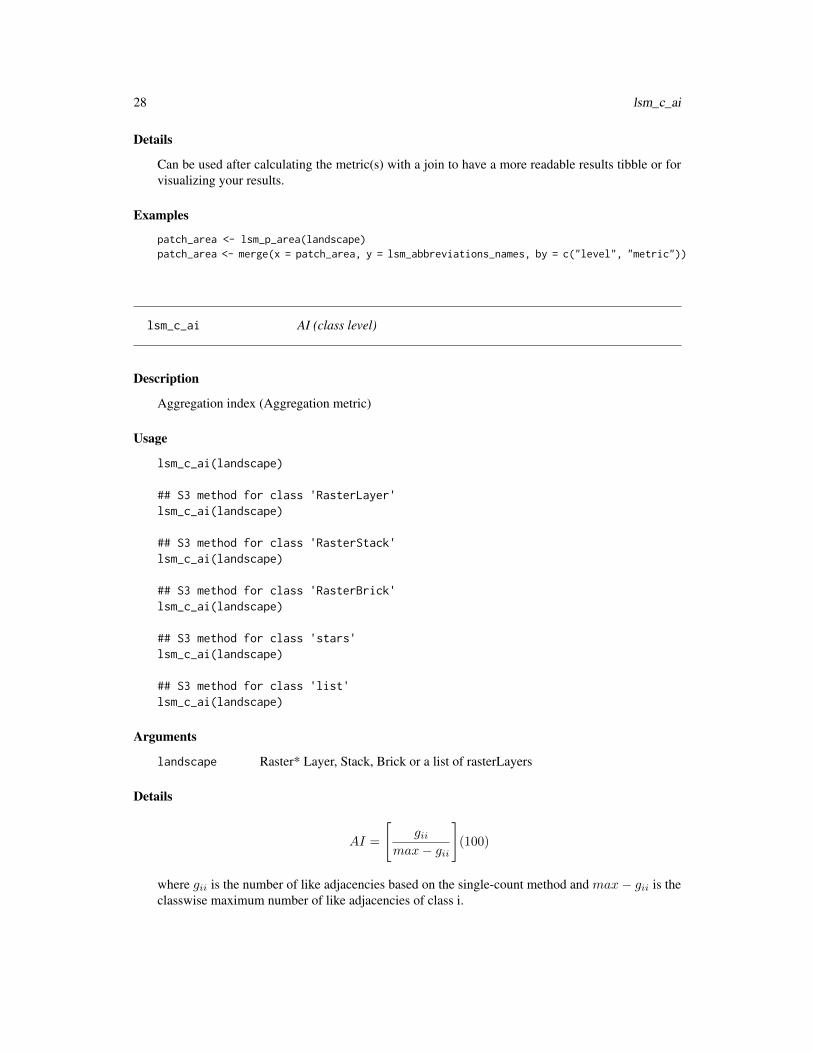
Can be used after calculating the metric(s) with a join to have a more readable results tibble or forvisualizing your results.

Examples

patch_area <- lsm_p_area(landscape)patch_area <- merge(x = patch_area, y = lsm_abbreviations_names, by = c("level", "metric"))

lsm_c_ai AI (class level)

Description

Aggregation index (Aggregation metric)

Usage

lsm_c_ai(landscape)

## S3 method for class 'RasterLayer'lsm_c_ai(landscape)

## S3 method for class 'RasterStack'lsm_c_ai(landscape)

## S3 method for class 'RasterBrick'lsm_c_ai(landscape)

## S3 method for class 'stars'lsm_c_ai(landscape)

## S3 method for class 'list'lsm_c_ai(landscape)

Arguments

landscape Raster* Layer, Stack, Brick or a list of rasterLayers

Details

AI =

[gii

max− gii

](100)

where gii is the number of like adjacencies based on the single-count method and max− gii is theclasswise maximum number of like adjacencies of class i.

lsm_c_area_cv 29

AI is an ’Aggregation metric’. It equals the number of like adjacencies divided by the theoreticalmaximum possible number of like adjacencies for that class. The metric is based on he adjacencymatrix and the the single-count method.

Units: Percent

Range: 0 <= AI <= 100

Behaviour: Equals 0 for maximally disaggregated and 100 for maximally aggregated classes.

Value

tibble

References


He, H. S., DeZonia, B. E., & Mladenoff, D. J. 2000. An aggregation index (AI) to quantify spatialpatterns of landscapes. Landscape ecology, 15(7), 591-601.

See Also

lsm_l_ai

Examples

lsm_c_ai(landscape)

lsm_c_area_cv AREA_CV (class level)

Description

Coefficient of variation of patch area (Area and edge metric)

Usage

lsm_c_area_cv(landscape, directions)

## S3 method for class 'RasterLayer'lsm_c_area_cv(landscape, directions = 8)

## S3 method for class 'RasterStack'lsm_c_area_cv(landscape, directions = 8)

30 lsm_c_area_cv

## S3 method for class 'RasterBrick'lsm_c_area_cv(landscape, directions = 8)

## S3 method for class 'stars'lsm_c_area_cv(landscape, directions = 8)

## S3 method for class 'list'lsm_c_area_cv(landscape, directions = 8)

Arguments

landscape Raster* Layer, Stack, Brick or a list of rasterLayersdirections The number of directions in which patches should be connected: 4 (rook’s case)

or 8 (queen’s case).

Details

AREACV = cv(AREA[patchij ])

where AREA[patchij ] is the area of each patch in hectares.

AREA_CV is an ’Area and Edge metric’. The metric summarises each class as the Coefficient ofvariation of all patch areas belonging to class i. The metric describes the differences among patchesof the same class i in the landscape and is easily comparable because it is scaled to the mean.

Units: Hectares

Range: AREA_CV >= 0

Behaviour: Equals AREA_CV = 0 if all patches are identical in size. Increases, without limit,as the variation of patch areas increases.

Value

tibble

References


See Also

lsm_p_area, cv,lsm_c_area_mn, lsm_c_area_sd,lsm_l_area_mn, lsm_l_area_sd, lsm_l_area_cv

Examples

lsm_c_area_cv(landscape)

lsm_c_area_mn 31

lsm_c_area_mn AREA_MN (class level)

Description

Mean of patch area (Area and edge metric)

Usage

lsm_c_area_mn(landscape, directions)

## S3 method for class 'RasterLayer'lsm_c_area_mn(landscape, directions = 8)

## S3 method for class 'RasterStack'lsm_c_area_mn(landscape, directions = 8)

## S3 method for class 'RasterBrick'lsm_c_area_mn(landscape, directions = 8)

## S3 method for class 'stars'lsm_c_area_mn(landscape, directions = 8)

## S3 method for class 'list'lsm_c_area_mn(landscape, directions = 8)

Arguments



Details

AREAMN = mean(AREA[patchij ])

where AREA[patchij ] is the area of each patch in hectares

AREA_MN is an ’Area and Edge metric’. The metric summarises each class as the mean of allpatch areas belonging to class i. The metric is a simple way to describe the composition of thelandscape. Especially together with the total class area (lsm_c_ca), it can also give an an idea ofpatch structure (e.g. many small patches vs. few larges patches).

Units: Hectares

Range: AREA_MN > 0

Behaviour: Approaches AREA_MN = 0 if all patches are small. Increases, without limit, as thepatch areas increase.

32 lsm_c_area_sd

Value

tibble

References


See Also

lsm_p_area, mean,lsm_c_area_cv, lsm_c_area_sd,lsm_l_area_mn, lsm_l_area_sd, lsm_l_area_cv

Examples

lsm_c_area_mn(landscape)

lsm_c_area_sd AREA_SD (class level)

Description

Standard deviation of patch area (Area and edge metric)

Usage

lsm_c_area_sd(landscape, directions)

## S3 method for class 'RasterLayer'lsm_c_area_sd(landscape, directions = 8)

## S3 method for class 'RasterStack'lsm_c_area_sd(landscape, directions = 8)

## S3 method for class 'RasterBrick'lsm_c_area_sd(landscape, directions = 8)

## S3 method for class 'stars'lsm_c_area_sd(landscape, directions = 8)

## S3 method for class 'list'lsm_c_area_sd(landscape, directions = 8)

## S3 method for class 'stars'lsm_c_division(landscape, directions = 8)

lsm_c_area_sd 33

Arguments



Details

AREASD = sd(AREA[patchij ])


AREA_SD is an ’Area and Edge metric’. The metric summarises each class as the standard devia-tion of all patch areas belonging to class i. The metric describes the differences among patches ofthe same class i in the landscape.

Units: Hectares

Range: AREA_SD >= 0

Behaviour: Equals AREA_SD = 0 if all patches are identical in size. Increases, without limit,as the variation of patch areas increases.

Value

tibble

References


See Also

lsm_p_area, sd,lsm_c_area_mn, lsm_c_area_cv,lsm_l_area_mn, lsm_l_area_sd, lsm_l_area_cv

Examples

lsm_c_area_sd(landscape)

34 lsm_c_ca

lsm_c_ca CA (class level)

Description

Total (class) area (Area and edge metric)

Usage

lsm_c_ca(landscape, directions)

## S3 method for class 'RasterLayer'lsm_c_ca(landscape, directions = 8)

## S3 method for class 'RasterStack'lsm_c_ca(landscape, directions = 8)

## S3 method for class 'RasterBrick'lsm_c_ca(landscape, directions = 8)

## S3 method for class 'stars'lsm_c_ca(landscape, directions = 8)

## S3 method for class 'list'lsm_c_ca(landscape, directions = 8)

Arguments

landscape Raster* Layer, Stack, Brick or a list of rasterLayers.directions The number of directions in which patches should be connected: 4 (rook’s case)


Details

CA = sum(AREA[patchij ])


CA is an ’Area and edge metric’ and a measure of composition. The total (class) area sums the areaof all patches belonging to class i. It shows if the landscape is e.g. dominated by one class or ifall classes are equally present. CA is an absolute measure, making comparisons among landscapeswith different total areas difficult.

Units: Hectares

Range: CA > 0

Behaviour: Approaches CA > 0 as the patch areas of class i become small. Increases, withoutlimit, as the patch areas of class i become large. CA = TA if only one class is present.

lsm_c_cai_cv 35

Value

tibble

References


See Also

lsm_p_area, sum,lsm_l_ta

Examples

lsm_c_ca(landscape)

lsm_c_cai_cv CAI_CV (class level)

Description

Coefficient of variation of core area index (Core area metric)

Usage

lsm_c_cai_cv(landscape, directions, consider_boundary, edge_depth)

## S3 method for class 'RasterLayer'lsm_c_cai_cv(landscape, directions = 8,consider_boundary = FALSE, edge_depth = 1)

## S3 method for class 'RasterStack'lsm_c_cai_cv(landscape, directions = 8,consider_boundary = FALSE, edge_depth = 1)

## S3 method for class 'RasterBrick'lsm_c_cai_cv(landscape, directions = 8,consider_boundary = FALSE, edge_depth = 1)

## S3 method for class 'stars'lsm_c_cai_cv(landscape, directions = 8,consider_boundary = FALSE, edge_depth = 1)

## S3 method for class 'list'lsm_c_cai_cv(landscape, directions = 8,consider_boundary = FALSE, edge_depth = 1)

36 lsm_c_cai_cv

Arguments



consider_boundary



Details

CAICV = cv(CAI[patchij ]

where CAI[patchij ] is the core area index of each patch.

CAI_CV is a ’Core area metric’. The metric summarises each class as the Coefficient of variationof the core area index of all patches belonging to class i. The core area index is the percentage ofcore area in relation to patch area. A cell is defined as core area if the cell has no neighbour with adifferent value than itself (rook’s case). The metric describes the differences among patches of thesame class i in the landscape. Because it is scaled to the mean, it is easily comparable.

Units: Percent

Range: CAI_CV >= 0

Behaviour: Equals CAI_CV = 0 if the core area index is identical for all patches. Increases,without limit, as the variation of the core area indices increases.

Value

tibble

References


See Also

lsm_p_cai, cv,lsm_c_cai_mn, lsm_c_cai_sd,lsm_l_cai_mn, lsm_l_cai_sd, lsm_l_cai_cv

Examples

lsm_c_cai_cv(landscape)

lsm_c_cai_mn 37

lsm_c_cai_mn CAI_MN (class level)

Description

Mean of core area index (Core area metric)

Usage

lsm_c_cai_mn(landscape, directions, consider_boundary, edge_depth)

## S3 method for class 'RasterLayer'lsm_c_cai_mn(landscape, directions = 8,consider_boundary = FALSE, edge_depth = 1)

## S3 method for class 'RasterStack'lsm_c_cai_mn(landscape, directions = 8,consider_boundary = FALSE, edge_depth = 1)

## S3 method for class 'RasterBrick'lsm_c_cai_mn(landscape, directions = 8,consider_boundary = FALSE, edge_depth = 1)

## S3 method for class 'stars'lsm_c_cai_mn(landscape, directions = 8,consider_boundary = FALSE, edge_depth = 1)

## S3 method for class 'list'lsm_c_cai_mn(landscape, directions = 8,consider_boundary = FALSE, edge_depth = 1)

Arguments



consider_boundary



Details

CAIMN = mean(CAI[patchij ]

38 lsm_c_cai_sd


CAI_MN is a ’Core area metric’. The metric summarises each class as the mean of the core areaindex of all patches belonging to class i. The core area index is the percentage of core area inrelation to patch area. A cell is defined as core area if the cell has no neighbour with a differentvalue than itself (rook’s case).

Units: Percent

Range: CAI_MN >= 0

Behaviour: Equals CAI_MN = 0 if CAI = 0 for all patches. Increases, without limit, as the corearea indices increase.

Value

tibble

References


See Also

lsm_p_cai, mean,lsm_c_cai_sd, lsm_c_cai_cv,lsm_l_cai_mn, lsm_l_cai_sd, lsm_l_cai_cv

Examples

lsm_c_cai_mn(landscape)

lsm_c_cai_sd CAI_SD (class level)

Description

Standard deviation of core area index (Core area metric)

lsm_c_cai_sd 39

Usage

lsm_c_cai_sd(landscape, directions, consider_boundary, edge_depth)

## S3 method for class 'RasterLayer'lsm_c_cai_sd(landscape, directions = 8,consider_boundary = FALSE, edge_depth = 1)

## S3 method for class 'RasterStack'lsm_c_cai_sd(landscape, directions = 8,consider_boundary = FALSE, edge_depth = 1)

## S3 method for class 'RasterBrick'lsm_c_cai_sd(landscape, directions = 8,consider_boundary = FALSE, edge_depth = 1)

## S3 method for class 'stars'lsm_c_cai_sd(landscape, directions = 8,consider_boundary = FALSE, edge_depth = 1)

## S3 method for class 'list'lsm_c_cai_sd(landscape, directions = 8,consider_boundary = FALSE, edge_depth = 1)

Arguments



consider_boundary



Details

CAISD = sd(CAI[patchij ]


CAI_SD is a ’Core area metric’. The metric summarises each class as the standard deviation of thecore area index of all patches belonging to class i. The core area index is the percentage of core areain relation to patch area. A cell is defined as core area if the cell has no neighbour with a differentvalue than itself (rook’s case). The metric describes the differences among patches of the same classi in the landscape.

Units: Percent

40 lsm_c_circle_cv

Range: CAI_SD >= 0

Behaviour: Equals CAI_SD = 0 if the core area index is identical for all patches. Increases,without limit, as the variation of core area indices increases.

Value

tibble

References


See Also

lsm_p_cai, sd,lsm_c_cai_mn, lsm_c_cai_cv,lsm_l_cai_mn, lsm_l_cai_sd, lsm_l_cai_cv

Examples

lsm_c_cai_sd(landscape)

lsm_c_circle_cv CIRCLE_CV (Class level)

Description

Coefficient of variation of related circumscribing circle (Shape metric)

Usage

lsm_c_circle_cv(landscape, directions)

## S3 method for class 'RasterLayer'lsm_c_circle_cv(landscape, directions = 8)

## S3 method for class 'RasterStack'lsm_c_circle_cv(landscape, directions = 8)

## S3 method for class 'RasterBrick'lsm_c_circle_cv(landscape, directions = 8)

## S3 method for class 'stars'lsm_c_circle_cv(landscape, directions = 8)

lsm_c_circle_cv 41

## S3 method for class 'list'lsm_c_circle_cv(landscape, directions = 8)

Arguments



Details

CIRCLECV = cv(CIRCLE[patchij ])

where CIRCLE[patchij ] is the related circumscribing circle of each patch.

CIRCLE_CV is a ’Shape metric’ and summarises each class as the Coefficient of variation of therelated circumscribing circle of all patches belonging to class i. CIRCLE describes the ratio betweenthe patch area and the smallest circumscribing circle of the patch and characterises the compactnessof the patch. CIRCLE_CV describes the differences among patches of the same class i in thelandscape. Because it is scaled to the mean, it is easily comparable.

Units: None

Range: CIRCLE_CV >= 0

Behaviour: Equals CIRCLE_CV if the related circumscribing circle is identical for all patches.Increases, without limit, as the variation of related circumscribing circles increases.

Value

tibble

References


Baker, W. L., and Y. Cai. 1992. The r.le programs for multiscale analysis of landscape structureusing the GRASS geographical information system. Landscape Ecology 7: 291-302.

See Also

lsm_p_circle, mean,lsm_c_circle_mn, lsm_c_circle_sd,lsm_l_circle_mn, lsm_l_circle_sd, lsm_l_circle_cv

Examples

lsm_c_circle_cv(landscape)

42 lsm_c_circle_mn

lsm_c_circle_mn CIRCLE_MN (Class level)

Description

Mean of related circumscribing circle (Shape metric)

Usage

lsm_c_circle_mn(landscape, directions)

## S3 method for class 'RasterLayer'lsm_c_circle_mn(landscape, directions = 8)

## S3 method for class 'RasterStack'lsm_c_circle_mn(landscape, directions = 8)

## S3 method for class 'RasterBrick'lsm_c_circle_mn(landscape, directions = 8)

## S3 method for class 'stars'lsm_c_circle_mn(landscape, directions = 8)

## S3 method for class 'list'lsm_c_circle_mn(landscape, directions = 8)

Arguments



Details

CIRCLEMN = mean(CIRCLE[patchij ])


CIRCLE_MN is a ’Shape metric’ and summarises each class as the mean of the related circum-scribing circle of all patches belonging to class i. CIRCLE describes the ratio between the patcharea and the smallest circumscribing circle of the patch and characterises the compactness of thepatch.

Units: None

Range: CIRCLE_MN > 0

Behaviour: Approaches CIRCLE_MN = 0 if the related circumscribing circle of all patches issmall. Increases, without limit, as the related circumscribing circles increase.

lsm_c_circle_sd 43

Value

tibble

References



See Also

lsm_p_circle, mean,lsm_c_circle_sd, lsm_c_circle_cv,lsm_l_circle_mn, lsm_l_circle_sd, lsm_l_circle_cv

Examples

lsm_c_circle_mn(landscape)

lsm_c_circle_sd CIRCLE_SD (Class level)

Description

Standard deviation of related circumscribing circle (Shape metric)

Usage

lsm_c_circle_sd(landscape, directions)

## S3 method for class 'RasterLayer'lsm_c_circle_sd(landscape, directions = 8)

## S3 method for class 'RasterStack'lsm_c_circle_sd(landscape, directions = 8)

## S3 method for class 'RasterBrick'lsm_c_circle_sd(landscape, directions = 8)

## S3 method for class 'stars'lsm_c_circle_sd(landscape, directions = 8)

## S3 method for class 'list'lsm_c_circle_sd(landscape, directions = 8)

44 lsm_c_circle_sd

Arguments



Details

CIRCLESD = sd(CIRCLE[patchij ])


CIRCLE_SD is a ’Shape metric’ and summarises each class as the standard deviation of the relatedcircumscribing circle of all patches belonging to class i. CIRCLE describes the ratio between thepatch area and the smallest circumscribing circle of the patch and characterises the compactness ofthe patch. The metric describes the differences among patches of the same class i in the landscape.

Units: None

Range: CIRCLE_SD >= 0

Behaviour: Equals CIRCLE_SD if the related circumscribing circle is identical for all patches.Increases, without limit, as the variation of related circumscribing circles increases.

Value

tibble

References



See Also

lsm_p_circle, mean,lsm_c_circle_mn, lsm_c_circle_cv,lsm_l_circle_mn, lsm_l_circle_sd, lsm_l_circle_cv

Examples

lsm_c_circle_sd(landscape)

lsm_c_clumpy 45

lsm_c_clumpy CLUMPY (class level)

Description

Clumpiness index (Aggregation metric)

Usage

lsm_c_clumpy(landscape)

## S3 method for class 'RasterLayer'lsm_c_clumpy(landscape)

## S3 method for class 'RasterStack'lsm_c_clumpy(landscape)

## S3 method for class 'RasterBrick'lsm_c_clumpy(landscape)

## S3 method for class 'stars'lsm_c_clumpy(landscape)

## S3 method for class 'list'lsm_c_clumpy(landscape)

Arguments


Details

GivenGi =

(gii

(m∑

k=1

gik)−minei

)

CLUMPY =

[Gi − Pi

PiforGi < Pi&Pi < .5; else

Gi − Pi

1− Pi

]

where gii is the number of like adjacencies, gik is the classwise number of all adjacencies includingthe focal class, minei is the minimum perimeter of the total class in terms of cell surfaces assumingtotal clumping and Pi is the proportion of landscape occupied by each class.

CLUMPY is an ’Aggregation metric’. It equals the proportional deviation of the proportion oflike adjacencies involving the corresponding class from that expected under a spatially randomdistribution. The metric is based on he adjacency matrix and the the double-count method.

46 lsm_c_cohesion

Units: None

, directions = directions

Range: -1 <= CLUMPY <= 1

Behaviour: Equals -1 for maximally disaggregated, 0 for randomly distributed and 1 for maxi-mally aggregated classes.

Value

tibble

References


Examples

lsm_c_clumpy(landscape)

lsm_c_cohesion COHESION (class level)

Description

Patch Cohesion Index (Aggregation metric)

Usage

lsm_c_cohesion(landscape, directions)

## S3 method for class 'RasterLayer'lsm_c_cohesion(landscape, directions = 8)

## S3 method for class 'RasterStack'lsm_c_cohesion(landscape, directions = 8)

## S3 method for class 'RasterBrick'lsm_c_cohesion(landscape, directions = 8)

## S3 method for class 'stars'lsm_c_cohesion(landscape, directions = 8)

## S3 method for class 'list'lsm_c_cohesion(landscape, directions = 8)

lsm_c_cohesion 47

Arguments



Details

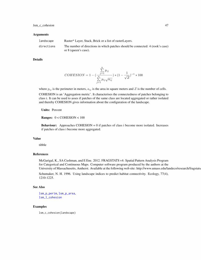
COHESION = 1− (

n∑j=1

pij

n∑j=1

pij√aij

) ∗ (1− 1√Z)−1 ∗ 100

where pij is the perimeter in meters, aij is the area in square meters and Z is the number of cells.

COHESION is an ’Aggregation metric’. It characterises the connectedness of patches belonging toclass i. It can be used to asses if patches of the same class are located aggregated or rather isolatedand thereby COHESION gives information about the configuration of the landscape.

Units: Percent

Ranges: 0 < COHESION < 100

Behaviour: Approaches COHESION = 0 if patches of class i become more isolated. Increasesif patches of class i become more aggregated.

Value

tibble

References


Schumaker, N. H. 1996. Using landscape indices to predict habitat connectivity. Ecology, 77(4),1210-1225.

See Also

lsm_p_perim, lsm_p_area,lsm_l_cohesion

Examples

lsm_c_cohesion(landscape)

48 lsm_c_contig_cv

lsm_c_contig_cv CONTIG_CV (class level)

Description

Coefficient of variation of Contiguity index (Shape metric)

Usage

lsm_c_contig_cv(landscape, directions)

## S3 method for class 'RasterLayer'lsm_c_contig_cv(landscape, directions = 8)

## S3 method for class 'RasterStack'lsm_c_contig_cv(landscape, directions = 8)

## S3 method for class 'RasterBrick'lsm_c_contig_cv(landscape, directions = 8)

## S3 method for class 'stars'lsm_c_contig_cv(landscape, directions = 8)

## S3 method for class 'list'lsm_c_contig_cv(landscape, directions = 8)

Arguments



Details

CONTIGCV = cv(CONTIG[patchij ])

where CONTIG[patchij ] is the contiguity of each patch.

CONTIG_CV is a ’Shape metric’. It summarises each class as the mean of each patch belonging toclass i. CONTIG_CV asses the spatial connectedness (contiguity) of cells in patches. The metriccoerces patch values to a value of 1 and the background to NA. A nine cell focal filter matrix:

filter_matrix <- matrix(c(1, 2, 1,2, 1, 2,1, 2, 1), 3, 3, byrow = T)

lsm_c_contig_mn 49

... is then used to weight orthogonally contiguous pixels more heavily than diagonally contiguouspixels. Therefore, larger and more connections between patch cells in the rookie case result in largercontiguity index values.

Units: None

Range: CONTIG_CV >= 0

Behaviour: CONTIG_CV = 0 if the contiguity index is identical for all patches. Increases,without limit, as the variation of CONTIG increases.

Value

tibble

References


LaGro, J. 1991. Assessing patch shape in landscape mosaics. Photogrammetric Engineering andRemote Sensing, 57(3), 285-293

See Also

lsm_p_contig, lsm_c_contig_mn, lsm_c_contig_cv,lsm_l_contig_mn, lsm_l_contig_sd, lsm_l_contig_cv

Examples

lsm_c_contig_cv(landscape)

lsm_c_contig_mn CONTIG_MN (class level)

Description

Mean of Contiguity index (Shape metric)

50 lsm_c_contig_mn

Usage

lsm_c_contig_mn(landscape, directions)

## S3 method for class 'RasterLayer'lsm_c_contig_mn(landscape, directions = 8)

## S3 method for class 'RasterStack'lsm_c_contig_mn(landscape, directions = 8)

## S3 method for class 'RasterBrick'lsm_c_contig_mn(landscape, directions = 8)

## S3 method for class 'stars'lsm_c_contig_mn(landscape, directions = 8)

## S3 method for class 'list'lsm_c_contig_mn(landscape, directions = 8)

Arguments



Details

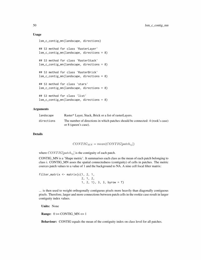
CONTIGMN = mean(CONTIG[patchij ])


CONTIG_MN is a ’Shape metric’. It summarises each class as the mean of each patch belonging toclass i. CONTIG_MN asses the spatial connectedness (contiguity) of cells in patches. The metriccoerces patch values to a value of 1 and the background to NA. A nine cell focal filter matrix:



Units: None

Range: 0 >= CONTIG_MN <= 1

Behaviour: CONTIG equals the mean of the contiguity index on class level for all patches.

lsm_c_contig_sd 51

Value

tibble

References



See Also

lsm_p_contig, lsm_c_contig_sd, lsm_c_contig_cv,lsm_l_contig_mn, lsm_l_contig_sd, lsm_l_contig_cv

Examples

lsm_c_contig_mn(landscape)

lsm_c_contig_sd CONTIG_SD (class level)

Description

Standard deviation of Contiguity index (Shape metric)

Usage

lsm_c_contig_sd(landscape, directions)

## S3 method for class 'RasterLayer'lsm_c_contig_sd(landscape, directions = 8)

## S3 method for class 'RasterStack'lsm_c_contig_sd(landscape, directions = 8)

## S3 method for class 'RasterBrick'lsm_c_contig_sd(landscape, directions = 8)

## S3 method for class 'stars'lsm_c_contig_sd(landscape, directions = 8)

## S3 method for class 'list'lsm_c_contig_sd(landscape, directions = 8)

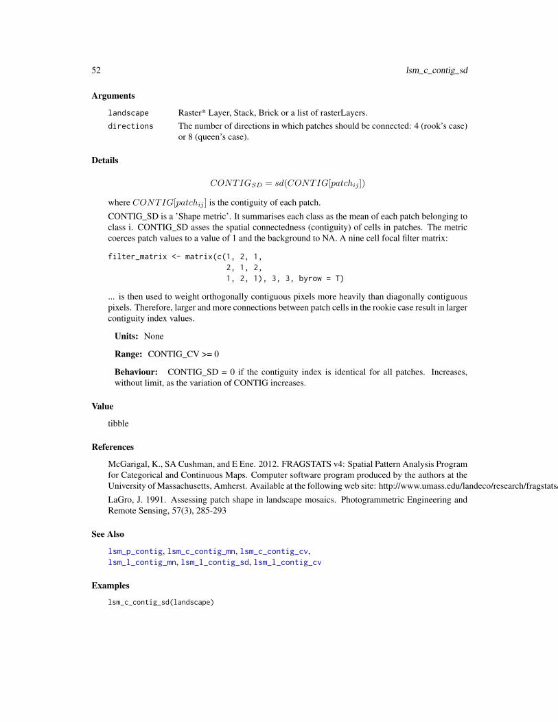
52 lsm_c_contig_sd

Arguments



Details

CONTIGSD = sd(CONTIG[patchij ])


CONTIG_SD is a ’Shape metric’. It summarises each class as the mean of each patch belonging toclass i. CONTIG_SD asses the spatial connectedness (contiguity) of cells in patches. The metriccoerces patch values to a value of 1 and the background to NA. A nine cell focal filter matrix:



Units: None


Behaviour: CONTIG_SD = 0 if the contiguity index is identical for all patches. Increases,without limit, as the variation of CONTIG increases.

Value

tibble

References



See Also

lsm_p_contig, lsm_c_contig_mn, lsm_c_contig_cv,lsm_l_contig_mn, lsm_l_contig_sd, lsm_l_contig_cv

Examples

lsm_c_contig_sd(landscape)

lsm_c_core_cv 53

lsm_c_core_cv CORE_CV (class level)

Description

Coefficient of variation of core area (Core area metric)

Usage

lsm_c_core_cv(landscape, directions, consider_boundary, edge_depth)

## S3 method for class 'RasterLayer'lsm_c_core_cv(landscape, directions = 8,consider_boundary = FALSE, edge_depth = 1)

## S3 method for class 'RasterStack'lsm_c_core_cv(landscape, directions = 8,consider_boundary = FALSE, edge_depth = 1)

## S3 method for class 'RasterBrick'lsm_c_core_cv(landscape, directions = 8,consider_boundary = FALSE, edge_depth = 1)

## S3 method for class 'stars'lsm_c_core_cv(landscape, directions = 8,consider_boundary = FALSE, edge_depth = 1)

## S3 method for class 'list'lsm_c_core_cv(landscape, directions = 8,consider_boundary = FALSE, edge_depth = 1)

Arguments



consider_boundary



Details

CORECV = cv(CORE[patchij ])

54 lsm_c_core_mn

where CORE[patchij ] is the core area in square meters of each patch.

CORE_CV is a ’Core area metric’. It equals the Coefficient of variation of the core area of eachpatch belonging to class i. The core area is defined as all cells that have no neighbour with adifferent value than themselves (rook’s case). The metric describes the differences among patchesof the same class i in the landscape and is easily comparable because it is scaled to the mean.

Units: Hectares

Range: CORE_CV >= 0

Behaviour: Equals CORE_CV = 0 if all patches have the same core area. Increases, withoutlimit, as the variation of patch core areas increases.

Value

tibble

References


See Also

lsm_p_core, cv,lsm_c_core_mn, lsm_c_core_sd,lsm_l_core_mn, lsm_l_core_sd, lsm_l_core_cv

Examples

lsm_c_core_cv(landscape)

lsm_c_core_mn CORE_MN (class level)

Description

Mean of core area (Core area metric)

lsm_c_core_mn 55

Usage

lsm_c_core_mn(landscape, directions, consider_boundary, edge_depth)

## S3 method for class 'RasterLayer'lsm_c_core_mn(landscape, directions = 8,consider_boundary = FALSE, edge_depth = 1)

## S3 method for class 'RasterStack'lsm_c_core_mn(landscape, directions = 8,consider_boundary = FALSE, edge_depth = 1)

## S3 method for class 'RasterBrick'lsm_c_core_mn(landscape, directions = 8,consider_boundary = FALSE, edge_depth = 1)

## S3 method for class 'stars'lsm_c_core_mn(landscape, directions = 8,consider_boundary = FALSE, edge_depth = 1)

## S3 method for class 'list'lsm_c_core_mn(landscape, directions = 8,consider_boundary = FALSE, edge_depth = 1)

Arguments


or 8 (queen’s case).consider_boundary



Details

COREMN = mean(CORE[patchij ])


CORE_MN is a ’Core area metric’ and equals the mean of core areas of all patches belonging toclass i. The core area is defined as all cells that have no neighbour with a different value thanthemselves (rook’s case).

Units: Hectares

Range: CORE_MN >= 0

Behaviour: Equals CORE_MN = 0 if CORE = 0 for all patches. Increases, without limit, as thecore area indices increase.

56 lsm_c_core_sd

Value

tibble

References


See Also

lsm_p_core, mean,lsm_c_core_sd, lsm_c_core_cv,lsm_l_core_mn, lsm_l_core_sd, lsm_l_core_cv

Examples

lsm_c_core_mn(landscape)

lsm_c_core_sd CORE_SD (class level)

Description

Standard deviation patch core area (class level)

Usage

lsm_c_core_sd(landscape, directions, consider_boundary, edge_depth)

## S3 method for class 'RasterLayer'lsm_c_core_sd(landscape, directions = 8,consider_boundary = FALSE, edge_depth = 1)

## S3 method for class 'RasterStack'lsm_c_core_sd(landscape, directions = 8,consider_boundary = FALSE, edge_depth = 1)

## S3 method for class 'RasterBrick'lsm_c_core_sd(landscape, directions = 8,consider_boundary = FALSE, edge_depth = 1)

## S3 method for class 'stars'lsm_c_core_sd(landscape, directions = 8,consider_boundary = FALSE, edge_depth = 1)

lsm_c_core_sd 57

## S3 method for class 'list'lsm_c_core_sd(landscape, directions = 8,consider_boundary = FALSE, edge_depth = 1)

Arguments



consider_boundary



Details

CORESD = sd(CORE[patchij ])


CORE_SD is a ’Core area metric’. It equals the standard deviation of the core area of each patchbelonging to class i. The core area is defined as all cells that have no neighbour with a differentvalue than themselves (rook’s case). The metric describes the differences among patches of thesame class i in the landscape.

Units: Hectares

Range: CORE_SD >= 0

Behaviour: Equals CORE_SD = 0 if all patches have the same core area. Increases, withoutlimit, as the variation of patch core areas increases.

Value

tibble

References


See Also

lsm_p_core, sd,lsm_c_core_mn, lsm_c_core_cv,lsm_l_core_mn, lsm_l_core_sd, lsm_l_core_cv

58 lsm_c_cpland

Examples

lsm_c_core_sd(landscape)

lsm_c_cpland CPLAND (class level)

Description

Core area percentage of landscape (Core area metric)

Usage

lsm_c_cpland(landscape, directions, consider_boundary, edge_depth)

## S3 method for class 'RasterLayer'lsm_c_cpland(landscape, directions = 8,consider_boundary = FALSE, edge_depth = 1)

## S3 method for class 'RasterStack'lsm_c_cpland(landscape, directions = 8,consider_boundary = FALSE, edge_depth = 1)

## S3 method for class 'RasterBrick'lsm_c_cpland(landscape, directions = 8,consider_boundary = FALSE, edge_depth = 1)

## S3 method for class 'stars'lsm_c_cpland(landscape, directions = 8,consider_boundary = FALSE, edge_depth = 1)

## S3 method for class 'list'lsm_c_cpland(landscape, directions = 8,consider_boundary = FALSE, edge_depth = 1)

Arguments



consider_boundary



lsm_c_dcad 59

Details

CPLAND = (

n∑j=1

acoreij

A) ∗ 100

where acoreij is the core area in square meters and A is the total landscape area in square meters.

CPLAND is a ’Core area metric’. It is the percentage of core area of class i in relation to the totallandscape area. A cell is defined as core area if the cell has no neighbour with a different value thanitself (rook’s case). Because CPLAND is a relative measure, it is comparable among landscapeswith different total areas.

Units: Percentage

Range: 0 <= CPLAND < 100

Behaviour: Approaches CPLAND = 0 if CORE = 0 for all patches. Increases as the amount ofcore area increases, i.e. patches become larger while being rather simple in shape.

Value

tibble

References


See Also

lsm_p_core and lsm_l_ta

Examples

lsm_c_cpland(landscape)

lsm_c_dcad DCAD (class level)

Description

Disjunct core area density (core area metric)

60 lsm_c_dcad

Usage

lsm_c_dcad(landscape, directions, consider_boundary, edge_depth)

## S3 method for class 'RasterLayer'lsm_c_dcad(landscape, directions = 8,consider_boundary = FALSE, edge_depth = 1)

## S3 method for class 'RasterStack'lsm_c_dcad(landscape, directions = 8,consider_boundary = FALSE, edge_depth = 1)

## S3 method for class 'RasterBrick'lsm_c_dcad(landscape, directions = 8,consider_boundary = FALSE, edge_depth = 1)

## S3 method for class 'stars'lsm_c_dcad(landscape, directions = 8,consider_boundary = FALSE, edge_depth = 1)

## S3 method for class 'list'lsm_c_dcad(landscape, directions = 8,consider_boundary = FALSE, edge_depth = 1)

Arguments



consider_boundary



Details

DCAD = (

n∑j=1

ncoreij

A) ∗ 10000 ∗ 100

where ncoreij is the number of disjunct core areas and A is the total landscape area in square meters.

DCAD is a ’Core area metric’. It equals the number of disjunct core areas per 100 ha relative tothe total area. A disjunct core area is a ’patch within the patch’ containing only core cells. A cell isdefined as core area if the cell has no neighbour with a different value than itself (rook’s case). Themetric is relative and therefore comparable among landscapes with different total areas.

Units: Number per 100 hectares

lsm_c_dcore_cv 61

Range: DCAD >= 0

Behaviour: Equals DCAD = 0 when DCORE = 0, i.e. no patch of class i contains a disjunct corearea. Increases, without limit, as disjunct core areas become more present, i.e. patches becominglarger and less complex.

Value

tibble

References


See Also

lsm_c_ndca, lsm_l_ta,lsm_l_dcad

Examples

lsm_c_dcad(landscape)

lsm_c_dcore_cv DCORE_CV (class level)

Description

Coefficient of variation number of disjunct core areas (Core area metric)

Usage

lsm_c_dcore_cv(landscape, directions, consider_boundary, edge_depth)

## S3 method for class 'RasterLayer'lsm_c_dcore_cv(landscape, directions = 8,consider_boundary = FALSE, edge_depth = 1)

## S3 method for class 'RasterStack'lsm_c_dcore_cv(landscape, directions = 8,consider_boundary = FALSE, edge_depth = 1)

## S3 method for class 'RasterBrick'lsm_c_dcore_cv(landscape, directions = 8,consider_boundary = FALSE, edge_depth = 1)

62 lsm_c_dcore_cv

## S3 method for class 'stars'lsm_c_dcore_cv(landscape, directions = 8,consider_boundary = FALSE, edge_depth = 1)

## S3 method for class 'list'lsm_c_dcore_cv(landscape, directions = 8,consider_boundary = FALSE, edge_depth = 1)

Arguments



consider_boundary



Details

DCORECV = cv(NCORE[patchij ])

where NCORE[patchij ] is the number of core areas.

DCORE_CV is an ’Core area metric’. It summarises each class as the Coefficient of variation ofall patch areas belonging to class i. A cell is defined as core if the cell has no neighbour with adifferent value than itself (rook’s case). NCORE counts the disjunct core areas, whereby a corearea is a ’patch within the patch’ containing only core cells. The metric describes the differencesamong patches of the same class i in the landscape and is easily comparable because it is scaled tothe mean.

Units: None

Range: DCORE_CV >= 0

Behaviour: Equals DCORE_CV = 0 if all patches have the same number of disjunct core areas.Increases, without limit, as the variation of number of disjunct core areas increases.

Value

tibble

References


lsm_c_dcore_mn 63

See Also

lsm_p_ncore, cv,lsm_c_dcore_mn, lsm_c_dcore_sd,lsm_l_dcore_mn, lsm_l_dcore_sd, lsm_l_dcore_cv

Examples

lsm_c_dcore_cv(landscape)

lsm_c_dcore_mn DCORE_MN (class level)

Description

Mean number of disjunct core areas (Core area metric)

Usage

lsm_c_dcore_mn(landscape, directions, consider_boundary, edge_depth)

## S3 method for class 'RasterLayer'lsm_c_dcore_mn(landscape, directions = 8,consider_boundary = FALSE, edge_depth = 1)

## S3 method for class 'RasterStack'lsm_c_dcore_mn(landscape, directions = 8,consider_boundary = FALSE, edge_depth = 1)

## S3 method for class 'RasterBrick'lsm_c_dcore_mn(landscape, directions = 8,consider_boundary = FALSE, edge_depth = 1)

## S3 method for class 'stars'lsm_c_dcore_mn(landscape, directions = 8,consider_boundary = FALSE, edge_depth = 1)

## S3 method for class 'list'lsm_c_dcore_mn(landscape, directions = 8,consider_boundary = FALSE, edge_depth = 1)

Arguments



64 lsm_c_dcore_mn

consider_boundary



Details

DCOREMN = mean(NCORE[patchij ])


DCORE_MN is an ’Core area metric’. It summarises each class as the mean of all patch areasbelonging to class i. A cell is defined as core if the cell has no neighbour with a different value thanitself (rook’s case). NCORE counts the disjunct core areas, whereby a core area is a ’patch withinthe patch’ containing only core cells.

Units: None

Range: DCORE_MN > 0

Behaviour: Equals DCORE_MN = 0 if NCORE = 0 for all patches. Increases, without limit, asthe number of disjunct core areas increases.

Value

tibble

References


See Also

lsm_p_ncore, mean,lsm_c_dcore_sd, lsm_c_dcore_cv,lsm_l_dcore_mn, lsm_l_dcore_sd, lsm_l_dcore_cv

Examples

lsm_c_dcore_mn(landscape)

lsm_c_dcore_sd 65

lsm_c_dcore_sd DCORE_SD (class level)

Description

Standard deviation number of disjunct core areas (Core area metric)

Usage

lsm_c_dcore_sd(landscape, directions, consider_boundary, edge_depth)

## S3 method for class 'RasterLayer'lsm_c_dcore_sd(landscape, directions = 8,consider_boundary = FALSE, edge_depth = 1)

## S3 method for class 'RasterStack'lsm_c_dcore_sd(landscape, directions = 8,consider_boundary = FALSE, edge_depth = 1)

## S3 method for class 'RasterBrick'lsm_c_dcore_sd(landscape, directions = 8,consider_boundary = FALSE, edge_depth = 1)

## S3 method for class 'stars'lsm_c_dcore_sd(landscape, directions = 8,consider_boundary = FALSE, edge_depth = 1)

## S3 method for class 'list'lsm_c_dcore_sd(landscape, directions = 8,consider_boundary = FALSE, edge_depth = 1)

Arguments



consider_boundary



Details

DCORESD = sd(NCORE[patchij ])

66 lsm_c_division


DCORE_SD is an ’Core area metric’. It summarises each class as the standard deviation of all patchareas belonging to class i. A cell is defined as core if the cell has no neighbour with a different valuethan itself (rook’s case). NCORE counts the disjunct core areas, whereby a core area is a ’patchwithin the patch’ containing only core cells. The metric describes the differences among patches ofthe same class i in the landscape.

Units: None

Range: DCORE_SD >= 0

Behaviour: Equals DCORE_SD = 0 if all patches have the same number of disjunct core areas.Increases, without limit, as the variation of number of disjunct core areas increases.

Value

tibble

References


See Also

lsm_p_ncore, sd,lsm_c_dcore_mn, lsm_c_dcore_cv,lsm_l_dcore_mn, lsm_l_dcore_sd, lsm_l_dcore_cv

Examples

lsm_c_dcore_sd(landscape)

lsm_c_division DIVISION (class level)

Description

Landscape division index (Aggregation metric)

lsm_c_division 67

Usage

lsm_c_division(landscape, directions)

## S3 method for class 'RasterLayer'lsm_c_division(landscape, directions = 8)

## S3 method for class 'RasterStack'lsm_c_division(landscape, directions = 8)

## S3 method for class 'RasterBrick'lsm_c_division(landscape, directions = 8)

## S3 method for class 'list'lsm_c_division(landscape, directions = 8)

Arguments



Details

DIV ISON = (1−n∑

j=1

(aijA

)2)

where aij is the area in square meters and A is the total landscape area in square meters.

DIVISION is an ’Aggregation metric. It can be in as the probability that two randomly selected cellsare not located in the same patch of class i. The landscape division index is negatively correlatedwith the effective mesh size (lsm_c_mesh).

Units: Proportion

Ranges: 0 <= Division < 1

Behaviour: Equals DIVISION = 0 if only one patch is present. Approaches DIVISION = 1 ifall patches of class i are single cells.

Value

tibble

References


Jaeger, J. A. 2000. Landscape division, splitting index, and effective mesh size: new measures oflandscape fragmentation. Landscape ecology, 15(2), 115-130.

68 lsm_c_ed

See Also

lsm_p_area, lsm_l_ta,lsm_l_division

Examples

lsm_c_division(landscape)

lsm_c_ed ED (class level)

Description

Edge Density (Area and Edge metric)

Usage

lsm_c_ed(landscape, count_boundary, directions)

## S3 method for class 'RasterLayer'lsm_c_ed(landscape, count_boundary = FALSE,directions = 8)

## S3 method for class 'RasterStack'lsm_c_ed(landscape, count_boundary = FALSE,directions = 8)

## S3 method for class 'RasterBrick'lsm_c_ed(landscape, count_boundary = FALSE,directions = 8)

## S3 method for class 'stars'lsm_c_ed(landscape, count_boundary = FALSE,directions = 8)

## S3 method for class 'list'lsm_c_ed(landscape, count_boundary = FALSE,directions = 8)

Arguments


count_boundary Count landscape boundary as edge.


lsm_c_ed 69

Details

ED =

m∑k=1

eik

A∗ 10000

where eik is the total edge length in meters and A is the total landscape area in square meters.

ED is an ’Area and Edge metric’. The edge density equals the sum of all edges of class i inrelation to the landscape area. The boundary of the landscape is only included in the correspondingtotal class edge length if count_boundary = TRUE. The metric describes the configuration of thelandscape, e.g. because an aggregation of the same class will result in a low edge density. Themetric is standardized to the total landscape area, and therefore comparisons among landscapeswith different total areas are possible.

Units: Meters per hectare

Range: ED >= 0

Behaviour: Equals ED = 0 if only one patch is present (and the landscape boundary is notincluded) and increases, without limit, as the landscapes becomes more patchy

Value

tibble

References


See Also

lsm_c_te, lsm_l_ta,lsm_l_ed

Examples

lsm_c_ed(landscape)

70 lsm_c_enn_cv

lsm_c_enn_cv ENN_CV (class level)

Description

Coefficient of variation of euclidean nearest-neighbor distance (Aggregation metric)

Usage

lsm_c_enn_cv(landscape, directions, verbose)

## S3 method for class 'RasterLayer'lsm_c_enn_cv(landscape, directions = 8,verbose = TRUE)

## S3 method for class 'RasterStack'lsm_c_enn_cv(landscape, directions = 8,verbose = TRUE)

## S3 method for class 'RasterBrick'lsm_c_enn_cv(landscape, directions = 8,verbose = TRUE)

## S3 method for class 'stars'lsm_c_enn_cv(landscape, directions = 8, verbose = TRUE)

## S3 method for class 'list'lsm_c_enn_cv(landscape, directions = 8, verbose = TRUE)

Arguments


or 8 (queen’s case).verbose Print warning message if not sufficient patches are present

Details

ENNCV = cv(ENN [patchij ])

where ENN [patchij ] is the euclidean nearest-neighbor distance of each patch.

ENN_CV is an ’Aggregation metric’. It summarises each class as the Coefficient of variation ofeach patch belonging to class i. ENN measures the distance to the nearest neighbouring patch ofthe same class i. The distance is measured from edge-to-edge. The range is limited by the cellresolution on the lower limit and the landscape extent on the upper limit. The metric is a simpleway to describe patch isolation. Because it is scaled to the mean, it is easily comparable amongdifferent landscapes.

lsm_c_enn_mn 71

Units: Meters

Range: ENN_CV >= 0

Behaviour: Equals ENN_CV = 0 if the euclidean nearest-neighbor distance is identical for allpatches. Increases, without limit, as the variation of ENN increases.

Value

tibble

References


McGarigal, K., and McComb, W. C. (1995). Relationships between landscape structure and breed-ing birds in the Oregon Coast Range. Ecological monographs, 65(3), 235-260.

See Also

lsm_p_enn, cv,lsm_c_enn_mn, lsm_c_enn_sd,lsm_l_enn_mn, lsm_l_enn_sd, lsm_l_enn_cv

Examples

lsm_c_enn_cv(landscape)

lsm_c_enn_mn ENN_MN (class level)

Description

Mean of euclidean nearest-neighbor distance (Aggregation metric)

Usage

lsm_c_enn_mn(landscape, directions, verbose)

## S3 method for class 'RasterLayer'lsm_c_enn_mn(landscape, directions = 8,verbose = TRUE)

## S3 method for class 'RasterStack'lsm_c_enn_mn(landscape, directions = 8,verbose = TRUE)

72 lsm_c_enn_mn

## S3 method for class 'RasterBrick'lsm_c_enn_mn(landscape, directions = 8,verbose = TRUE)

## S3 method for class 'stars'lsm_c_enn_mn(landscape, directions = 8, verbose = TRUE)

## S3 method for class 'list'lsm_c_enn_mn(landscape, directions = 8, verbose = TRUE)

Arguments



verbose Print warning message if not sufficient patches are present

Details

ENNMN = mean(ENN [patchij ])


ENN_MN is an ’Aggregation metric’. It summarises each class as the mean of each patch belongingto class i. ENN measures the distance to the nearest neighbouring patch of the same class i. Thedistance is measured from edge-to-edge. The range is limited by the cell resolution on the lowerlimit and the landscape extent on the upper limit.

Units: Meters

Range: ENN_MN > 0

Behaviour: Approaches ENN_MN = 0 as the distance to the nearest neighbour decreases, i.e.patches of the same class i are more aggregated. Increases, without limit, as the distance betweenneighbouring patches of the same class i increases, i.e. patches are more isolated.

Value

tibble

References



lsm_c_enn_sd 73

See Also

lsm_p_enn, mean,lsm_c_enn_sd, lsm_c_enn_cv,lsm_l_enn_mn, lsm_l_enn_sd, lsm_l_enn_cv

Examples

lsm_c_enn_mn(landscape)

lsm_c_enn_sd ENN_SD (class level)

Description

Standard deviation of euclidean nearest-neighbor distance (Aggregation metric)

Usage

lsm_c_enn_sd(landscape, directions, verbose)

## S3 method for class 'RasterLayer'lsm_c_enn_sd(landscape, directions = 8,verbose = TRUE)

## S3 method for class 'RasterStack'lsm_c_enn_sd(landscape, directions = 8,verbose = TRUE)

## S3 method for class 'RasterBrick'lsm_c_enn_sd(landscape, directions = 8,verbose = TRUE)

## S3 method for class 'stars'lsm_c_enn_sd(landscape, directions = 8, verbose = TRUE)

## S3 method for class 'list'lsm_c_enn_sd(landscape, directions = 8, verbose = TRUE)

Arguments




74 lsm_c_enn_sd

Details

ENNSD = sd(ENN [patchij ])


ENN_CV is an ’Aggregation metric’. It summarises each class as the standard deviation of eachpatch belonging to class i. ENN measures the distance to the nearest neighbouring patch of the sameclass i. The distance is measured from edge-to-edge. The range is limited by the cell resolution onthe lower limit and the landscape extent on the upper limit. The metric is a simple way to describepatch isolation. Because it is scaled to the mean, it is easily comparable among different landscapes.

Units: Meters

Range: ENN_SD >= 0

Behaviour: Equals ENN_SD = 0 if the euclidean nearest-neighbor distance is identical for allpatches. Increases, without limit, as the variation of ENN increases.

Value

tibble

References



See Also

lsm_p_enn, sd,lsm_c_enn_mn, lsm_c_enn_cv,lsm_l_enn_mn, lsm_l_enn_sd, lsm_l_enn_cv

Examples

lsm_c_enn_sd(landscape)

lsm_c_frac_cv 75

lsm_c_frac_cv FRAC_CV (class level)

Description

Coefficient of variation fractal dimension index (Shape metric)

Usage

lsm_c_frac_cv(landscape, directions)

## S3 method for class 'RasterLayer'lsm_c_frac_cv(landscape, directions = 8)

## S3 method for class 'RasterStack'lsm_c_frac_cv(landscape, directions = 8)

## S3 method for class 'RasterBrick'lsm_c_frac_cv(landscape, directions = 8)

## S3 method for class 'stars'lsm_c_frac_cv(landscape, directions = 8)

## S3 method for class 'list'lsm_c_frac_cv(landscape, directions = 8)

Arguments



Details

FRACCV = cv(FRAC[patchij ])

where FRAC[patchij ] equals the fractal dimension index of each patch.

FRAC_CV is a ’Shape metric’. The metric summarises each class as the Coefficient of variation ofthe fractal dimension index of all patches belonging to class i. The fractal dimension index is basedon the patch perimeter and the patch area and describes the patch complexity. The Coefficient ofvariation is scaled to the mean and comparable among different landscapes.

Units: None

Range: FRAC_CV >= 0

Behaviour: Equals FRAC_CV = 0 if the fractal dimension index is identical for all patches.Increases, without limit, as the variation of the fractal dimension indices increases.

76 lsm_c_frac_mn

Value

tibble

References


Mandelbrot, B. B. 1977. Fractals: Form, Chance, and Dimension. San Francisco. W. H. Freemanand Company.

See Also

lsm_p_frac, cv,lsm_c_frac_mn, lsm_c_frac_sd,lsm_l_frac_mn, lsm_l_frac_sd, lsm_l_frac_cv

Examples

lsm_c_frac_cv(landscape)

lsm_c_frac_mn FRAC_MN (class level)

Description

Mean fractal dimension index (Shape metric)

Usage

lsm_c_frac_mn(landscape, directions)

## S3 method for class 'RasterLayer'lsm_c_frac_mn(landscape, directions = 8)

## S3 method for class 'RasterStack'lsm_c_frac_mn(landscape, directions = 8)

## S3 method for class 'RasterBrick'lsm_c_frac_mn(landscape, directions = 8)

## S3 method for class 'stars'lsm_c_frac_mn(landscape, directions = 8)

## S3 method for class 'list'lsm_c_frac_mn(landscape, directions = 8)

lsm_c_frac_mn 77

Arguments



Details

FRACMN = mean(FRAC[patchij ])


FRAC_MN is a ’Shape metric’. The metric summarises each class as the mean of the fractal di-mension index of all patches belonging to class i. The fractal dimension index is based on the patchperimeter and the patch area and describes the patch complexity. The Coefficient of variation isscaled to the mean and comparable among different landscapes.

Units: None

Range: FRAC_MN > 0

Behaviour: Approaches FRAC_MN = 1 if all patches are squared and FRAC_MN = 2 if allpatches are irregular.

References



See Also

lsm_p_frac, mean,lsm_c_frac_sd, lsm_c_frac_cv,lsm_l_frac_mn, lsm_l_frac_sd, lsm_l_frac_cv

Examples

lsm_c_frac_mn(landscape)

78 lsm_c_frac_sd

lsm_c_frac_sd FRAC_SD (class level)

Description

Standard deviation fractal dimension index (Shape metric)

Usage

lsm_c_frac_sd(landscape, directions)

## S3 method for class 'RasterLayer'lsm_c_frac_sd(landscape, directions = 8)

## S3 method for class 'RasterStack'lsm_c_frac_sd(landscape, directions = 8)

## S3 method for class 'RasterBrick'lsm_c_frac_sd(landscape, directions = 8)

## S3 method for class 'stars'lsm_c_frac_sd(landscape, directions = 8)

## S3 method for class 'list'lsm_c_frac_sd(landscape, directions = 8)

Arguments



Details

FRACSD = sd(FRAC[patchij ])


FRAC_SD is a ’Shape metric’. The metric summarises each class as the standard deviation of thefractal dimension index of all patches belonging to class i. The fractal dimension index is based onthe patch perimeter and the patch area and describes the patch complexity.

Units: None

Range: FRAC_SD>= 0

Behaviour: Equals FRAC_SD = 0 if the fractal dimension index is identical for all patches.Increases, without limit, as the variation of the fractal dimension indices increases.

lsm_c_gyrate_cv 79

Value

tibble

References



See Also

lsm_p_frac, sd,lsm_c_frac_mn, lsm_c_frac_cv,lsm_l_frac_mn, lsm_l_frac_sd, lsm_l_frac_cv

Examples

lsm_c_frac_sd(landscape)

lsm_c_gyrate_cv GYRATE_CV (class level)

Description

Coefficient of variation radius of gyration (Area and edge metric)

Usage

lsm_c_gyrate_cv(landscape, directions)

## S3 method for class 'RasterLayer'lsm_c_gyrate_cv(landscape, directions = 8)

## S3 method for class 'RasterStack'lsm_c_gyrate_cv(landscape, directions = 8)

## S3 method for class 'RasterBrick'lsm_c_gyrate_cv(landscape, directions = 8)

## S3 method for class 'stars'lsm_c_gyrate_cv(landscape, directions = 8)

## S3 method for class 'list'lsm_c_gyrate_cv(landscape, directions = 8)

80 lsm_c_gyrate_cv

Arguments



Details

GY RATECV = cv(GY RATE[patchij ])

where GY RATE[patchij ] equals the radius of gyration of each patch.

GYRATE_CV is an ’Area and edge metric’. The metric summarises each class as the Coefficientof variation of the radius of gyration of all patches belonging to class i. GYRATE measures thedistance from each cell to the patch centroid and is based on cell center-to-cell center distances.The metrics characterises both the patch area and compactness. The Coefficient of variation isscaled to the mean and comparable among different landscapes.

Units: Meters

Range: GYRATE_CV >= 0

Behaviour: Equals GYRATE_CV = 0 if the radius of gyration is identical for all patches. In-creases, without limit, as the variation of the radius of gyration increases.

Value

tibble

References


Keitt, T. H., Urban, D. L., & Milne, B. T. 1997. Detecting critical scales in fragmented landscapes.Conservation ecology, 1(1).

See Also

lsm_p_gyrate, cv,lsm_c_gyrate_mn, lsm_c_gyrate_sd,lsm_l_gyrate_mn, lsm_l_gyrate_sd, lsm_l_gyrate_cv

Examples

lsm_c_gyrate_cv(landscape)

lsm_c_gyrate_mn 81

lsm_c_gyrate_mn GYRATE_MN (class level)

Description

Mean radius of gyration (Area and edge metric)

Usage

lsm_c_gyrate_mn(landscape, directions)

## S3 method for class 'RasterLayer'lsm_c_gyrate_mn(landscape, directions = 8)

## S3 method for class 'RasterStack'lsm_c_gyrate_mn(landscape, directions = 8)

## S3 method for class 'RasterBrick'lsm_c_gyrate_mn(landscape, directions = 8)

## S3 method for class 'stars'lsm_c_gyrate_mn(landscape, directions = 8)

## S3 method for class 'list'lsm_c_gyrate_mn(landscape, directions = 8)

Arguments



Details

GY RATEMN = mean(GY RATE[patchij ])

where GY RATE[patchij ] equals the radius of gyration of each patch.GYRATE_MN is an ’Area and edge metric’. The metric summarises each class as the mean ofthe radius of gyration of all patches belonging to class i. GYRATE measures the distance fromeach cell to the patch centroid and is based on cell center-to-cell center distances. The metricscharacterises both the patch area and compactness. The Coefficient of variation is scaled to themean and comparable among different landscapes.

Units: Meters

Range: GYRATE_MN >= 0

Behaviour: Approaches GYRATE_MN = 0 if every patch is a single cell. Increases, withoutlimit, when only one patch is present.

82 lsm_c_gyrate_sd

Value

tibble

References



See Also

lsm_p_gyrate, mean,lsm_c_gyrate_sd, lsm_c_gyrate_cv,lsm_l_gyrate_mn, lsm_l_gyrate_sd, lsm_l_gyrate_cv

Examples

lsm_c_gyrate_mn(landscape)

lsm_c_gyrate_sd GYRATE_SD (class level)

Description

Standard deviation radius of gyration (Area and edge metric)

Usage

lsm_c_gyrate_sd(landscape, directions)

## S3 method for class 'RasterLayer'lsm_c_gyrate_sd(landscape, directions = 8)

## S3 method for class 'RasterStack'lsm_c_gyrate_sd(landscape, directions = 8)

## S3 method for class 'RasterBrick'lsm_c_gyrate_sd(landscape, directions = 8)

## S3 method for class 'stars'lsm_c_gyrate_sd(landscape, directions = 8)

## S3 method for class 'list'lsm_c_gyrate_sd(landscape, directions = 8)

lsm_c_gyrate_sd 83

Arguments



Details

GY RATESD = sd(GY RATE[patchij ])


GYRATE_SD is an ’Area and edge metric’. The metric summarises each class as the standarddeviation of the radius of gyration of all patches belonging to class i. GYRATE measures thedistance from each cell to the patch centroid and is based on cell center-to-cell center distances.The metrics characterises both the patch area and compactness.

Units: Meters

Range: GYRATE_SD >= 0

Behaviour: Equals GYRATE_SD = 0 if the radius of gyration is identical for all patches. In-creases, without limit, as the variation of the radius of gyration increases.

Value

tibble

References



See Also

lsm_p_gyrate, cv,lsm_c_gyrate_mn, lsm_c_gyrate_cv,lsm_l_gyrate_mn, lsm_l_gyrate_sd, lsm_l_gyrate_cv

Examples

lsm_c_gyrate_sd(landscape)

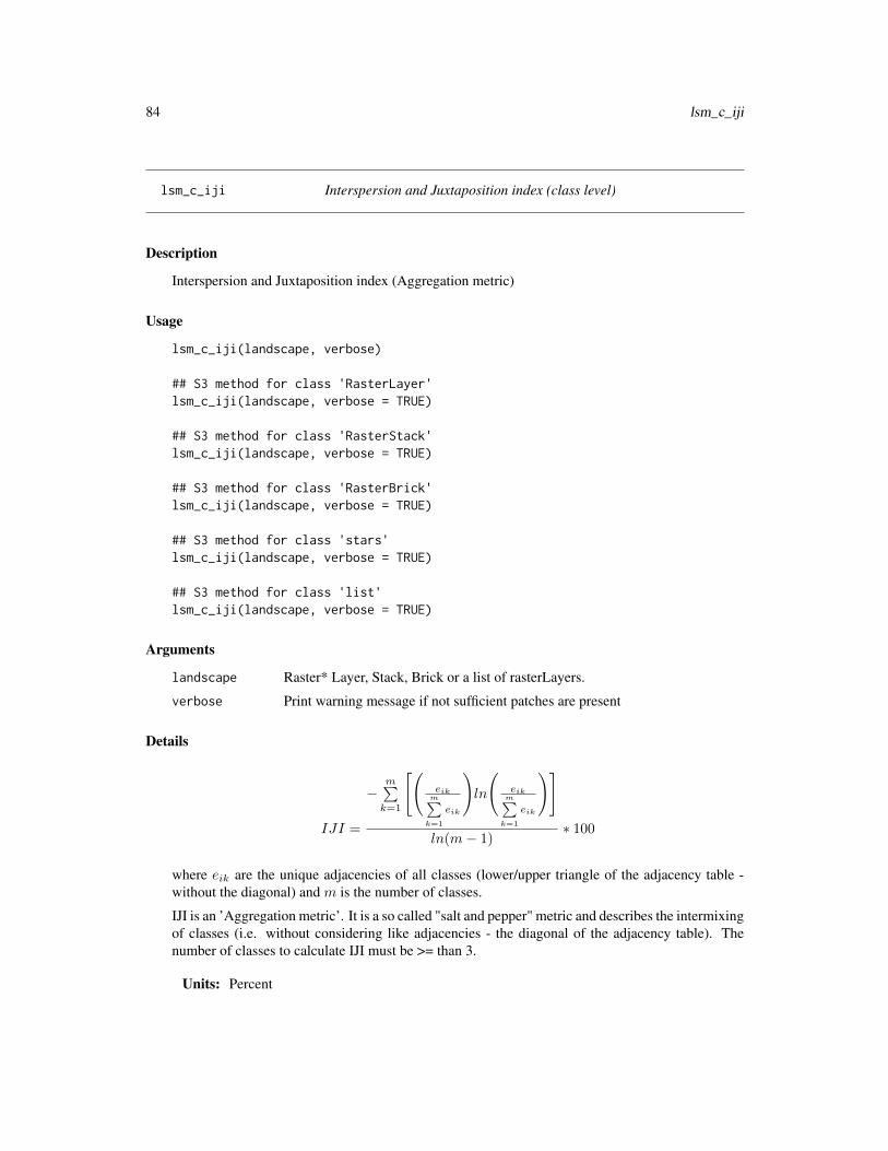
84 lsm_c_iji

lsm_c_iji Interspersion and Juxtaposition index (class level)

Description

Interspersion and Juxtaposition index (Aggregation metric)

Usage

lsm_c_iji(landscape, verbose)

## S3 method for class 'RasterLayer'lsm_c_iji(landscape, verbose = TRUE)

## S3 method for class 'RasterStack'lsm_c_iji(landscape, verbose = TRUE)

## S3 method for class 'RasterBrick'lsm_c_iji(landscape, verbose = TRUE)

## S3 method for class 'stars'lsm_c_iji(landscape, verbose = TRUE)

## S3 method for class 'list'lsm_c_iji(landscape, verbose = TRUE)

Arguments



Details

IJI =

−m∑

k=1

[(eik

m∑k=1

eik

)ln

(eik

m∑k=1

eik

)]

ln(m− 1)∗ 100

where eik are the unique adjacencies of all classes (lower/upper triangle of the adjacency table -without the diagonal) and m is the number of classes.

IJI is an ’Aggregation metric’. It is a so called "salt and pepper" metric and describes the intermixingof classes (i.e. without considering like adjacencies - the diagonal of the adjacency table). Thenumber of classes to calculate IJI must be >= than 3.

Units: Percent

lsm_c_lpi 85

Range: 0 < IJI <= 100

Behaviour: Approaches 0 if a class is only adjacent to a single other class and equals 100 whena class is equally adjacent to all other classes.

Value

tibble

References


McGarigal, K., & Marks, B. J. 1995. FRAGSTATS: spatial pattern analysis program for quanti-fying landscape structure. Gen. Tech. Rep. PNW-GTR-351. Portland, OR: US Department ofAgriculture, Forest Service, Pacific Northwest Research Station. 122 p, 351.

See Also

lsm_l_iji

Examples

lsm_c_iji(landscape)

lsm_c_lpi LPI (class level)

Description

Largest patch index (Area and Edge metric)

Usage

lsm_c_lpi(landscape, directions)

## S3 method for class 'RasterLayer'lsm_c_lpi(landscape, directions = 8)

## S3 method for class 'RasterStack'lsm_c_lpi(landscape, directions = 8)

## S3 method for class 'RasterBrick'lsm_c_lpi(landscape, directions = 8)

## S3 method for class 'stars'lsm_c_lpi(landscape, directions = 8)

86 lsm_c_lpi

## S3 method for class 'list'lsm_c_lpi(landscape, directions = 8)

Arguments



Details

LPI =

nmaxj=1

(aij)

A∗ 100

where max(aij) is the area of the patch in square meters and A is the total landscape area in squaremeters.

The largest patch index is an ’Area and edge metric’. It is the percentage of the landscape coveredby the corresponding largest patch of each class i. It is a simple measure of dominance.

Units: Percentage

Range: 0 < LPI <= 100

Behaviour: Approaches LPI = 0 when the largest patch is becoming small and equals LPI = 100when only one patch is present

Value

tibble

References


See Also

lsm_p_area, lsm_l_ta,lsm_l_lpi

Examples

lsm_c_lpi(landscape)

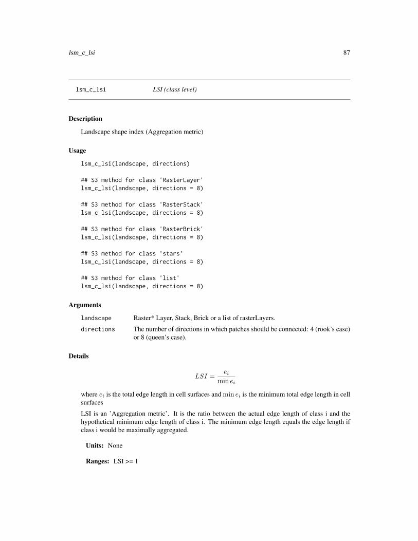
lsm_c_lsi 87

lsm_c_lsi LSI (class level)

Description

Landscape shape index (Aggregation metric)

Usage

lsm_c_lsi(landscape, directions)

## S3 method for class 'RasterLayer'lsm_c_lsi(landscape, directions = 8)

## S3 method for class 'RasterStack'lsm_c_lsi(landscape, directions = 8)

## S3 method for class 'RasterBrick'lsm_c_lsi(landscape, directions = 8)

## S3 method for class 'stars'lsm_c_lsi(landscape, directions = 8)

## S3 method for class 'list'lsm_c_lsi(landscape, directions = 8)

Arguments



Details

LSI =ei

min ei

where ei is the total edge length in cell surfaces and min ei is the minimum total edge length in cellsurfaces

LSI is an ’Aggregation metric’. It is the ratio between the actual edge length of class i and thehypothetical minimum edge length of class i. The minimum edge length equals the edge length ifclass i would be maximally aggregated.

Units: None

Ranges: LSI >= 1

88 lsm_c_mesh

Behaviour: Equals LSI = 1 when only one squared patch is present or all patches are maximallyaggregated. Increases, without limit, as the length of the actual edges increases, i.e. the patchesbecome less compact.

Value

tibble

References


Patton, D. R. 1975. A diversity index for quantifying habitat "edge". Wildl. Soc.Bull. 3:171-173.

See Also

lsm_p_shape,lsm_l_lsi

Examples

lsm_c_lsi(landscape)

lsm_c_mesh MESH (class level)

Description

Effective Mesh Size (Aggregation metric)

Usage

lsm_c_mesh(landscape, directions)

## S3 method for class 'RasterLayer'lsm_c_mesh(landscape, directions = 8)

## S3 method for class 'RasterStack'lsm_c_mesh(landscape, directions = 8)

## S3 method for class 'RasterBrick'lsm_c_mesh(landscape, directions = 8)

## S3 method for class 'stars'lsm_c_mesh(landscape, directions = 8)

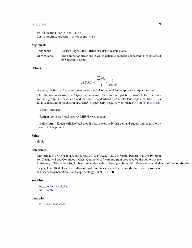
lsm_c_mesh 89

## S3 method for class 'list'lsm_c_mesh(landscape, directions = 8)

Arguments



Details

MESH =

n∑j=1

a2ij

A∗ 1

10000

where aij is the patch area in square meters and A is the total landscape area in square meters.

The effective mesh size is an ’Aggregation metric’. Because each patch is squared before the sumsfor each group i are calculated and the sum is standardized by the total landscape area, MESH is arelative measure of patch structure. MESH is perfectly, negatively correlated to lsm_c_division.

Units: Hectares

Range: cell size / total area <= MESH <= total area

Behaviour: Equals cellsize/total area if class covers only one cell and equals total area if onlyone patch is present.

Value

tibble

References



See Also

lsm_p_area, lsm_l_ta,lsm_l_mesh

Examples

lsm_c_mesh(landscape)

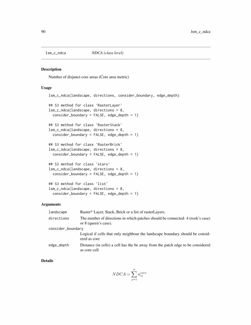
90 lsm_c_ndca

lsm_c_ndca NDCA (class level)

Description

Number of disjunct core areas (Core area metric)

Usage

lsm_c_ndca(landscape, directions, consider_boundary, edge_depth)

## S3 method for class 'RasterLayer'lsm_c_ndca(landscape, directions = 8,consider_boundary = FALSE, edge_depth = 1)

## S3 method for class 'RasterStack'lsm_c_ndca(landscape, directions = 8,consider_boundary = FALSE, edge_depth = 1)

## S3 method for class 'RasterBrick'lsm_c_ndca(landscape, directions = 8,consider_boundary = FALSE, edge_depth = 1)

## S3 method for class 'stars'lsm_c_ndca(landscape, directions = 8,consider_boundary = FALSE, edge_depth = 1)

## S3 method for class 'list'lsm_c_ndca(landscape, directions = 8,consider_boundary = FALSE, edge_depth = 1)

Arguments



consider_boundary



Details

NDCA =

n∑j=1

ncoreij

lsm_c_nlsi 91

where ncoreij is the number of disjunct core areas.

NDCA is a ’Core area metric’. The metric summarises class i as the sum of all patches belongingto class i. A cell is defined as core if the cell has no neighbour with a different value than itself(rook’s case). NDCA counts the disjunct core areas, whereby a core area is a ’patch within thepatch’ containing only core cells. It describes patch area and shape simultaneously (more core areawhen the patch is large, however, the shape must allow disjunct core areas). Thereby, a compactshape (e.g. a square) will contain less disjunct core areas than a more irregular patch.

Units: None

Range: NDCA >= 0

Behaviour: NDCA = 0 when TCA = 0, i.e. every cell in patches of class i is an edge. NDCAincreases, with out limit, as core area increases and patch shapes allow disjunct core areas (i.e.patch shapes become rather complex).

Value

tibble

References


See Also

lsm_c_tca,lsm_p_ncore, lsm_l_ndca

Examples

lsm_c_ndca(landscape)

lsm_c_nlsi nLSI (class level)

Description

Normalized landscape shape index (Aggregation metric)

92 lsm_c_nlsi

Usage

lsm_c_nlsi(landscape, directions)

## S3 method for class 'RasterLayer'lsm_c_nlsi(landscape, directions = 8)

## S3 method for class 'RasterStack'lsm_c_nlsi(landscape, directions = 8)

## S3 method for class 'RasterBrick'lsm_c_nlsi(landscape, directions = 8)

## S3 method for class 'stars'lsm_c_nlsi(landscape, directions = 8)

## S3 method for class 'list'lsm_c_nlsi(landscape, directions = 8)

Arguments



Details

nLSI =ei

min ei

where ei is the total edge length in cell surfaces and min ei is the minimum total edge length in cellsurfaces

nLSI is an ’Aggregation metric’. It is the ratio between the actual edge length of class i and thehypothetical minimum edge length of class i. The minimum edge length equals the edge length ifclass i would be maximally aggregated.

Units: None

Ranges: nlsi >= 1

Behaviour: Equals nlsi = 1 when only one squared patch is present or all patches are maximallyaggregated. Increases, without limit, as the length of the actual edges increases, i.e. the patchesbecome less compact.

Value

tibble

lsm_c_np 93

References



See Also

lsm_p_shape

Examples

lsm_c_nlsi(landscape)

lsm_c_np NP (class level)

Description

Number of patches (Aggregation metric)

Usage

lsm_c_np(landscape, directions)

## S3 method for class 'RasterLayer'lsm_c_np(landscape, directions = 8)

## S3 method for class 'RasterStack'lsm_c_np(landscape, directions = 8)

## S3 method for class 'RasterBrick'lsm_c_np(landscape, directions = 8)

## S3 method for class 'stars'lsm_c_np(landscape, directions = 8)

## S3 method for class 'list'lsm_c_np(landscape, directions = 8)

Arguments



94 lsm_c_pafrac

Details

NP = ni

where ni is the number of patches.

NP is an ’Aggregation metric’. It describes the fragmentation of a class, however, does not neces-sarily contain information about the configuration or composition of the class.

Units: None

Ranges: NP >= 1

Behaviour: Equals NP = 1 when only one patch is present and increases, without limit, as thenumber of patches increases

Value

tibble

References


See Also

lsm_l_np

Examples

lsm_c_np(landscape)

lsm_c_pafrac PAFRAC (class level)

Description

Perimeter-Area Fractal Dimension (Shape metric)

lsm_c_pafrac 95

Usage

lsm_c_pafrac(landscape, directions, verbose)

## S3 method for class 'RasterLayer'lsm_c_pafrac(landscape, directions = 8,verbose = TRUE)

## S3 method for class 'RasterStack'lsm_c_pafrac(landscape, directions = 8,verbose = TRUE)

## S3 method for class 'RasterBrick'lsm_c_pafrac(landscape, directions = 8,verbose = TRUE)

## S3 method for class 'stars'lsm_c_pafrac(landscape, directions = 8, verbose = TRUE)

## S3 method for class 'list'lsm_c_pafrac(landscape, directions = 8, verbose = TRUE)

Arguments



Details

PAFRAC =2

β

where β is the slope of the regression of the area against the perimeter (logarithm) nin∑

j=1

ln aij =

a+ βnin∑

j=1

ln pij

PAFRAC is a ’Shape metric’. It describes the patch complexity of class i while being scale indepen-dent. This means that increasing the patch size while not changing the patch form will not changethe metric. However, it is only meaningful if the relationship between the area and perimeter islinear on a logarithmic scale. Furthermore, if there are less than 10 patches in class i, the metricreturns NA because of the small-sample issue.

Units: None

Range: 1 <= PAFRAC <= 2

Behaviour: Approaches PAFRAC = 1 for patches with simple shapes and approaches PAFRAC= 2 for irregular shapes

96 lsm_c_para_cv

Value

tibble

References


Burrough, P. A. 1986. Principles of Geographical Information Systems for Land Resources Assess-ment. Monographs on Soil and Resources Survey No. 12. Clarendon Press, Oxford

See Also

lsm_p_area, lsm_p_perim,lsm_l_pafrac

Examples

lsm_c_pafrac(landscape)

lsm_c_para_cv PARA_CV (class level)

Description

Coefficient of variation perimeter-area ratio (Shape metric)

Usage

lsm_c_para_cv(landscape, directions)

## S3 method for class 'RasterLayer'lsm_c_para_cv(landscape, directions = 8)

## S3 method for class 'RasterStack'lsm_c_para_cv(landscape, directions = 8)

## S3 method for class 'RasterBrick'lsm_c_para_cv(landscape, directions = 8)

## S3 method for class 'stars'lsm_c_para_cv(landscape, directions = 8)

## S3 method for class 'list'lsm_c_para_cv(landscape, directions = 8)

lsm_c_para_cv 97

Arguments



Details

PARACV = cv(PARA[patchij ]

where PARA[patchij ] is the perimeter area ratio of each patch.

PARA_CV is a ’Shape metric’. It summarises each class as the Coefficient of variation of each patchbelonging to class i. The perimeter-area ratio describes the patch complexity in a straightforwardway. However, because it is not standarised to a certain shape (e.g. a square), it is not scaleindependent, meaning that increasing the patch size while not changing the patch form will changethe ratio.

Units: None

Range: PARA_CV >= 0

Behaviour: Equals PARA_CV = 0 if the perimeter-area ratio is identical for all patches. In-creases, without limit, as the variation of the perimeter-area ratio increases.

Value

tibble

References


See Also

lsm_p_para, cv,lsm_c_para_mn, lsm_c_para_sd,lsm_l_para_mn, lsm_l_para_sd, lsm_l_para_cv

Examples

lsm_c_para_cv(landscape)

98 lsm_c_para_mn

lsm_c_para_mn PARA_MN (class level)

Description

Mean perimeter-area ratio (Shape metric)

Usage

lsm_c_para_mn(landscape, directions)

## S3 method for class 'RasterLayer'lsm_c_para_mn(landscape, directions = 8)

## S3 method for class 'RasterStack'lsm_c_para_mn(landscape, directions = 8)

## S3 method for class 'RasterBrick'lsm_c_para_mn(landscape, directions = 8)

## S3 method for class 'stars'lsm_c_para_mn(landscape, directions = 8)

## S3 method for class 'list'lsm_c_para_mn(landscape, directions = 8)

Arguments



Details

PARAMN = mean(PARA[patchij ]

where PARA[patchij ] is the perimeter area ratio of each patch.PARA_MN is a ’Shape metric’. It summarises each class as the mean of each patch belonging toclass i. The perimeter-area ratio describes the patch complexity in a straightforward way. However,because it is not standarised to a certain shape (e.g. a square), it is not scale independent, meaningthat increasing the patch size while not changing the patch form will change the ratio.

Units: None

Range: PARA_MN > 0

Behaviour: Approaches PARA_MN > 0 if PARA for each patch approaches PARA > 0, i.e. theform approaches a rather small square. Increases, without limit, as PARA increases, i.e. patchesbecome more complex.

lsm_c_para_sd 99

Value

tibble

References


See Also

lsm_p_para, mean,lsm_c_para_sd, lsm_c_para_cv,lsm_l_para_mn, lsm_l_para_sd, lsm_l_para_cv

Examples

lsm_c_para_mn(landscape)

lsm_c_para_sd PARA_SD (class level)

Description

Standard deviation perimeter-area ratio (Shape metric)

Usage

lsm_c_para_sd(landscape, directions)

## S3 method for class 'RasterLayer'lsm_c_para_sd(landscape, directions = 8)

## S3 method for class 'RasterStack'lsm_c_para_sd(landscape, directions = 8)

## S3 method for class 'RasterBrick'lsm_c_para_sd(landscape, directions = 8)

## S3 method for class 'stars'lsm_c_para_sd(landscape, directions = 8)

## S3 method for class 'list'lsm_c_para_sd(landscape, directions = 8)

100 lsm_c_para_sd

Arguments



Details

PARASD = sd(PARA[patchij ]


PARA_SD is a ’Shape metric’. It summarises each class as the standard deviation of each patchbelonging to class i. The perimeter-area ratio describes the patch complexity in a straightforwardway. However, because it is not standarised to a certain shape (e.g. a square), it is not scaleindependent, meaning that increasing the patch size while not changing the patch form will changethe ratio.

Units: None

Range: PARA_SD >= 0

Behaviour: Equals PARA_SD = 0 if the perimeter-area ratio is identical for all patches. In-creases, without limit, as the variation of the perimeter-area ratio increases.

Value

tibble

References


See Also

lsm_p_para, sd,lsm_c_para_mn, lsm_c_para_cv,lsm_l_para_mn, lsm_l_para_sd, lsm_l_para_cv

Examples

lsm_c_para_sd(landscape)

lsm_c_pd 101

lsm_c_pd PD (class level)

Description

Patch density (Aggregation metric)

Usage

lsm_c_pd(landscape, directions)

## S3 method for class 'RasterLayer'lsm_c_pd(landscape, directions = 8)

## S3 method for class 'RasterStack'lsm_c_pd(landscape, directions = 8)

## S3 method for class 'RasterBrick'lsm_c_pd(landscape, directions = 8)

## S3 method for class 'stars'lsm_c_pd(landscape, directions = 8)

## S3 method for class 'list'lsm_c_pd(landscape, directions = 8)

Arguments



Details

PD =niA∗ 10000 ∗ 100

where ni is the number of patches and A is the total landscape area in square meters.

PD is an ’Aggregation metric’. It describes the fragmentation of a class, however, does not nec-essarily contain information about the configuration or composition of the class. In contrast tolsm_c_np it is standardized to the area and comparisons among landscapes with different total areaare possible.


Ranges: 0 < PD <= 1e+06

Behaviour: Increases as the landscape gets more patchy. Reaches its maximum if every cell is adifferent patch.

102 lsm_c_pladj

Value

tibble

References


See Also

lsm_c_np, lsm_l_ta,lsm_l_pd

Examples

lsm_c_pd(landscape)

lsm_c_pladj PLADJ (class level)

Description

Percentage of Like Adjacencies (Aggregation metric)

Usage

lsm_c_pladj(landscape)

## S3 method for class 'RasterLayer'lsm_c_pladj(landscape)

## S3 method for class 'RasterStack'lsm_c_pladj(landscape)

## S3 method for class 'RasterBrick'lsm_c_pladj(landscape)

## S3 method for class 'stars'lsm_c_pladj(landscape)

## S3 method for class 'list'lsm_c_pladj(landscape)

Arguments


lsm_c_pland 103

Details

PLADJ = (gij

m∑k=1

gik

) ∗ 100

where gii is the number of adjacencies between cells of class i and gik is the number of adjacenciesbetween cells of class i and k.

PLADJ is an ’Aggregation metric’. It calculates the frequency how often patches of different classesi (focal class) and k are next to each other, and following is a measure of class aggregation. Theadjacencies are counted using the double-count method.

Units: Percent

Ranges: 0 <= PLADJ <= 100

Behaviour: Equals PLADJ = 0 if class i is maximal disaggregated, i.e. every cell is a differentpatch. Equals PLADJ = 100 when the only one patch is present.

Value

tibble

References

McGarigal, K., SA Cushman, and E Ene. 2012. FRAGSTATS v4: Spatial Pattern Analysis Programfor Categorical and Continuous Maps. Computer software program produced by the authors at theUniversity of Massachusetts, Amherst. Available at the following web site: http://www.umass.edu/landeco/research/fragstats/fragstats.html.

Examples

lsm_c_pladj(landscape)

lsm_c_pland PLAND (class level)

Description

Percentage of landscape of class (Area and Edge metric)

104 lsm_c_pland

Usage

lsm_c_pland(landscape, directions)

## S3 method for class 'RasterLayer'lsm_c_pland(landscape, directions = 8)

## S3 method for class 'RasterStack'lsm_c_pland(landscape, directions = 8)

## S3 method for class 'RasterBrick'lsm_c_pland(landscape, directions = 8)

## S3 method for class 'stars'lsm_c_pland(landscape, directions = 8)

## S3 method for class 'list'lsm_c_pland(landscape, directions = 8)

Arguments



Details

PLAND =

n∑j=1

aij

A∗ 100

where aij is the area of each patch and A is the total landscape area.

PLAND is an ’Area and edge metric’. It is the percentage of the landscape belonging to class i.It is a measure of composition and because of the relative character directly comparable amonglandscapes with different total areas.

Units: Percentage

Range: 0 < PLAND <= 100

Behaviour: Approaches PLAND = 0 when the proportional class area is decreasing. EqualsPLAND = 100 when only one patch is present.

Value

tibble

lsm_c_shape_cv 105

References


See Also

lsm_c_ca, lsm_l_ta

Examples

lsm_c_pland(landscape)

lsm_c_shape_cv SHAPE_CV (class level)

Description

Covariance of variation shape index (Shape metric)

Usage

lsm_c_shape_cv(landscape, directions)

## S3 method for class 'RasterLayer'lsm_c_shape_cv(landscape, directions = 8)

## S3 method for class 'RasterStack'lsm_c_shape_cv(landscape, directions = 8)

## S3 method for class 'RasterBrick'lsm_c_shape_cv(landscape, directions = 8)

## S3 method for class 'stars'lsm_c_shape_cv(landscape, directions = 8)

## S3 method for class 'list'lsm_c_shape_cv(landscape, directions = 8)

Arguments



106 lsm_c_shape_cv

Details

SHAPECV = cv(SHAPE[patchij ])

where SHAPE[patchij ] is the shape index of each patch.

SHAPE_CV is a ’Shape metric’. Each class is summarised as the Coefficient of variation of eachpatch belonging to class i. SHAPE describes the ratio between the actual perimeter of the patch andthe hypothetical minimum perimeter of the patch. The minimum perimeter equals the perimeter ifthe patch would be maximally compact.

Units: None

Range: SHAPE_CV >= 0

Behaviour: Equals SHAPE_CV = 0 if all patches have an identical shape index. Increases,without limit, as the variation of the shape index increases.

Value

tibble

References



See Also

lsm_p_shape, cv,lsm_c_shape_mn, lsm_c_shape_sd,lsm_l_shape_mn, lsm_l_shape_sd, lsm_l_shape_cv

Examples

lsm_c_shape_cv(landscape)

lsm_c_shape_mn 107

lsm_c_shape_mn SHAPE_MN (class level)

Description

Mean shape index (Shape metric)

Usage

lsm_c_shape_mn(landscape, directions)

## S3 method for class 'RasterLayer'lsm_c_shape_mn(landscape, directions = 8)

## S3 method for class 'RasterStack'lsm_c_shape_mn(landscape, directions = 8)

## S3 method for class 'RasterBrick'lsm_c_shape_mn(landscape, directions = 8)

## S3 method for class 'stars'lsm_c_shape_mn(landscape, directions = 8)

## S3 method for class 'list'lsm_c_shape_mn(landscape, directions = 8)

Arguments



Details

SHAPEMN = mean(SHAPE[patchij ])


SHAPE_MN is a ’Shape metric’. Each class is summarised as the mean of each patch belonging toclass i. SHAPE describes the ratio between the actual perimeter of the patch and the hypotheticalminimum perimeter of the patch. The minimum perimeter equals the perimeter if the patch wouldbe maximally compact.

Units: None

Range: SHAPE_SD >= 1

Behaviour: Equals SHAPE_MN = 0 if all patches are squares. Increases, without limit, as theshapes of patches become more complex.

108 lsm_c_shape_sd

Value

tibble

References



See Also

lsm_p_shape, mean,lsm_c_shape_sd, lsm_c_shape_cv,lsm_l_shape_mn, lsm_l_shape_sd, lsm_l_shape_cv

Examples

lsm_c_shape_mn(landscape)

lsm_c_shape_sd SHAPE_SD (class level)

Description

Standard deviation shape index (Shape metric)

Usage

lsm_c_shape_sd(landscape, directions)

## S3 method for class 'RasterLayer'lsm_c_shape_sd(landscape, directions = 8)

## S3 method for class 'RasterStack'lsm_c_shape_sd(landscape, directions = 8)

## S3 method for class 'RasterBrick'lsm_c_shape_sd(landscape, directions = 8)

## S3 method for class 'stars'lsm_c_shape_sd(landscape, directions = 8)

## S3 method for class 'list'lsm_c_shape_sd(landscape, directions = 8)

lsm_c_shape_sd 109

Arguments



Details

SHAPESD = sd(SHAPE[patchij ])


SHAPE_SD is a ’Shape metric’. Each class is summarised as the standard deviation of each patchbelonging to class i. SHAPE describes the ratio between the actual perimeter of the patch and thehypothetical minimum perimeter of the patch. The minimum perimeter equals the perimeter if thepatch would be maximally compact.

Units: None


Behaviour: Equals SHAPE_SD = 0 if all patches have an identical shape index. Increases,without limit, as the variation of the shape index increases.

Value

tibble

References



See Also

lsm_p_shape, sd,lsm_c_shape_mn, lsm_c_shape_cv,lsm_l_shape_mn, lsm_l_shape_sd, lsm_l_shape_cv

Examples

lsm_c_shape_sd(landscape)

110 lsm_c_split

lsm_c_split SPLIT (class level)

Description

Splitting index (Aggregation metric)

Usage

lsm_c_split(landscape, directions)

## S3 method for class 'RasterLayer'lsm_c_split(landscape, directions = 8)

## S3 method for class 'RasterStack'lsm_c_split(landscape, directions = 8)

## S3 method for class 'RasterBrick'lsm_c_split(landscape, directions = 8)

## S3 method for class 'stars'lsm_c_split(landscape, directions = 8)

## S3 method for class 'list'lsm_c_split(landscape, directions = 8)

Arguments



Details

SPLIT =A2

n∑j=1

a2ij

where aij is the patch area in square meters and A is the total landscape area.

SPLIT is an ’Aggregation metric’. It describes the number of patches if all patches of class i wouldbe divided into equally sized patches.

Units: None

Range: 1 <= SPLIT <= Number of cells squared

Behaviour: Equals SPLIT = 1 if only one patch is present. Increases as the number of patchesof class i increases and is limited if all cells are a patch

lsm_c_tca 111

Value

tibble

References



See Also

lsm_p_area, lsm_l_ta,lsm_l_split

Examples

lsm_c_split(landscape)

lsm_c_tca TCA (class level)

Description

Total core area (Core area metric)

Usage

lsm_c_tca(landscape, directions, consider_boundary, edge_depth)

## S3 method for class 'RasterLayer'lsm_c_tca(landscape, directions = 8,consider_boundary = FALSE, edge_depth = 1)

## S3 method for class 'RasterStack'lsm_c_tca(landscape, directions = 8,consider_boundary = FALSE, edge_depth = 1)

## S3 method for class 'RasterBrick'lsm_c_tca(landscape, directions = 8,consider_boundary = FALSE, edge_depth = 1)

## S3 method for class 'stars'lsm_c_tca(landscape, directions = 8,consider_boundary = FALSE, edge_depth = 1)

112 lsm_c_tca

## S3 method for class 'list'lsm_c_tca(landscape, directions = 8,consider_boundary = FALSE, edge_depth = 1)

Arguments



consider_boundary



Details

TCA =

n∑j=1

acoreij ∗ ( 1

10000)

where here acoreij is the core area in square meters.

TCA is a ’Core area metric’ and equals the sum of core areas of all patches belonging to class i.A cell is defined as core area if the cell has no neighbour with a different value than itself (rook’scase). In other words, the core area of a patch is all area that is not an edge. It characterises patchareas and shapes of patches belonging to class i simultaneously (more core area when the patchis large and the shape is rather compact, i.e. a square). Additionally, TCA is a measure for theconfiguration of the landscape, because the sum of edges increase as patches are less aggregated.

Units: Hectares

Range: TCA >= 0

Behaviour: Increases, without limit, as patch areas increase and patch shapes simplify. TCA =0 when every cell in every patch of class i is an edge.

Value

tibble

References


See Also

lsm_p_core, lsm_l_tca

lsm_c_te 113

Examples

lsm_c_tca(landscape)

lsm_c_te TE (class level)

Description

Total (class) edge (Area and Edge metric)

Usage

lsm_c_te(landscape, count_boundary, directions)

## S3 method for class 'RasterLayer'lsm_c_te(landscape, count_boundary = FALSE,directions = 8)

## S3 method for class 'RasterStack'lsm_c_te(landscape, count_boundary = FALSE,directions = 8)

## S3 method for class 'RasterBrick'lsm_c_te(landscape, count_boundary = FALSE,directions = 8)

## S3 method for class 'stars'lsm_c_te(landscape, count_boundary = FALSE,directions = 8)

## S3 method for class 'list'lsm_c_te(landscape, count_boundary = FALSE,directions = 8)

Arguments


count_boundary Include landscape boundary in edge length


114 lsm_l_ai

Details

TE =

m∑k=1

eik

where eik is the edge lengths in meters. TE is an ’Area and edge metric’. Total (class) edgeincludes all edges between class i and all other classes k. It measures the configuration of thelandscape because a highly fragmented landscape will have many edges. However, total edge isan absolute measure, making comparisons among landscapes with different total areas difficult. Ifcound_boundary = TRUE also edges to the landscape boundary are included.

Units: Meters

Range: TE >= 0

Behaviour: Equals TE = 0 if all cells are edge cells. Increases, without limit, as landscapebecomes more fragmented

Value

tibble

References


See Also

lsm_p_perim lsm_l_te

Examples

lsm_c_te(landscape)

lsm_l_ai AI (landscape level)

Description

Aggregation index (Aggregation metric)

lsm_l_ai 115

Usage

lsm_l_ai(landscape)

## S3 method for class 'RasterLayer'lsm_l_ai(landscape)

## S3 method for class 'RasterStack'lsm_l_ai(landscape)

## S3 method for class 'RasterBrick'lsm_l_ai(landscape)

## S3 method for class 'stars'lsm_l_ai(landscape)

## S3 method for class 'list'lsm_l_ai(landscape)

Arguments


Details

AI =

[m∑i=1

( giimax− gii

)Pi

](100)

where gii is the number of like adjacencies based on the single-count method and max − gii isthe classwise maximum number of like adjacencies of class i and Pi the proportion of landscapecompromised of class i.

AI is an ’Aggregation metric’. It equals the number of like adjacencies divided by the theoreticalmaximum possible number of like adjacencies for that class summed over each class for the entirelandscape. The metric is based on he adjacency matrix and the the single-count method.

Units: Percent

Range: 0 <= AI <= 100

Behaviour: Equals 0 for maximally disaggregated and 100 for maximally aggregated classes.

Value

tibble

116 lsm_l_area_cv

References


He, H. S., DeZonia, B. E., & Mladenoff, D. J. 2000. An aggregation index (AI) to quantify spatialpatterns of landscapes. Landscape ecology, 15(7), 591-601.

See Also

lsm_c_ai

Examples

lsm_l_ai(landscape)

lsm_l_area_cv AREA_CV (landscape level)

Description

Coefficient of variation of patch area (Area and edge metric)

Usage

lsm_l_area_cv(landscape, directions)

## S3 method for class 'RasterLayer'lsm_l_area_cv(landscape, directions = 8)

## S3 method for class 'RasterStack'lsm_l_area_cv(landscape, directions = 8)

## S3 method for class 'RasterBrick'lsm_l_area_cv(landscape, directions = 8)

## S3 method for class 'stars'lsm_l_area_cv(landscape, directions = 8)

## S3 method for class 'list'lsm_l_area_cv(landscape, directions = 8)

Arguments



lsm_l_area_mn 117

Details

AREACV = cv(AREA[patchij ])


AREA_CV is an ’Area and Edge metric’. The metric summarises the landscape as the Coefficientof variation of all patches in the landscape. The metric describes the differences among patches inthe landscape and is easily comparable because it is scaled to the mean.

Units: Hectares

Range: AREA_CV >= 0

Behaviour: Equals AREA_CV = 0 if all patches are identical in size. Increases, without limit,as the variation of patch areas increases.

Value

tibble

References


See Also

lsm_p_area, cv,lsm_c_area_mn, lsm_c_area_sd, lsm_c_area_cv,lsm_l_area_mn, lsm_l_area_sd

Examples

lsm_l_area_cv(landscape)

lsm_l_area_mn AREA_MN (landscape level)

Description

Mean of patch area (Area and edge metric)

118 lsm_l_area_mn

Usage

lsm_l_area_mn(landscape, directions)

## S3 method for class 'RasterLayer'lsm_l_area_mn(landscape, directions = 8)

## S3 method for class 'RasterStack'lsm_l_area_mn(landscape, directions = 8)

## S3 method for class 'RasterBrick'lsm_l_area_mn(landscape, directions = 8)

## S3 method for class 'stars'lsm_l_area_mn(landscape, directions = 8)

## S3 method for class 'list'lsm_l_area_mn(landscape, directions = 8)

Arguments



Details

AREAMN = mean(AREA[patchij ])

where AREA[patchij ] is the area of each patch in hectares

AREA_MN is an ’Area and Edge metric’. The metric summarises the landscape as the mean of allpatch in the landscape. The metric is a simple way to describe the composition of the landscape.Especially together with the total landscape area (lsm_l_ta), it can also give an an idea of patchstructure (e.g. many small patches vs. few larges patches).

Units: Hectares

Range: AREA_MN > 0

Behaviour: Approaches AREA_MN = 0 if all patches are small. Increases, without limit, as thepatch areas increase.

Value

tibble

References


lsm_l_area_sd 119

See Also

lsm_p_area, mean,lsm_c_area_mn, lsm_c_area_sd, lsm_c_area_cvlsm_l_area_sd, lsm_l_area_cv

Examples

lsm_l_area_mn(landscape)

lsm_l_area_sd AREA_SD (landscape level)

Description

Standard deviation of patch area (Area and edge metric)

Usage

lsm_l_area_sd(landscape, directions)

## S3 method for class 'RasterLayer'lsm_l_area_sd(landscape, directions = 8)

## S3 method for class 'RasterStack'lsm_l_area_sd(landscape, directions = 8)

## S3 method for class 'RasterBrick'lsm_l_area_sd(landscape, directions = 8)

## S3 method for class 'stars'lsm_l_area_sd(landscape, directions = 8)

## S3 method for class 'list'lsm_l_area_sd(landscape, directions = 8)

Arguments



120 lsm_l_cai_cv

Details

AREASD = sd(AREA[patchij ])


AREA_SD is an ’Area and Edge metric’. The metric summarises the landscape as the standarddeviation of all patch in the landscape. The metric describes the differences among all patches inthe landscape.

Units: Hectares

Range: AREA_SD >= 0

Behaviour: Equals AREA_SD = 0 if all patches are identical in size. Increases, without limit,as the variation of patch areas increases.

Value

tibble

References


See Also

lsm_p_area, sd,lsm_c_area_mn, lsm_c_area_sd, lsm_c_area_cvlsm_l_area_mn, lsm_l_area_cv

Examples

lsm_l_area_sd(landscape)

lsm_l_cai_cv CAI_CV (landscape level)

Description

Coefficient of variation of core area index (Core area metric)

lsm_l_cai_cv 121

Usage

lsm_l_cai_cv(landscape, directions, consider_boundary, edge_depth)

## S3 method for class 'RasterLayer'lsm_l_cai_cv(landscape, directions = 8,consider_boundary = FALSE, edge_depth = 1)

## S3 method for class 'RasterStack'lsm_l_cai_cv(landscape, directions = 8,consider_boundary = FALSE, edge_depth = 1)

## S3 method for class 'RasterBrick'lsm_l_cai_cv(landscape, directions = 8,consider_boundary = FALSE, edge_depth = 1)

## S3 method for class 'stars'lsm_l_cai_cv(landscape, directions = 8,consider_boundary = FALSE, edge_depth = 1)

## S3 method for class 'list'lsm_l_cai_cv(landscape, directions = 8,consider_boundary = FALSE, edge_depth = 1)

Arguments



consider_boundary



Details

CAICV = cv(CAI[patchij ]


CAI_CV is a ’Core area metric’. The metric summarises the landscape as the Coefficient of varia-tion of the core area index of all patches in the landscape. The core area index is the percentage ofcore area in relation to patch area. A cell is defined as core area if the cell has no neighbour with adifferent value than itself (rook’s case). The metric describes the differences among all patches inthe landscape. Because it is scaled to the mean, it is easily comparable.

Units: Percent

122 lsm_l_cai_mn

Range: CAI_CV >= 0

Behaviour: Equals CAI_CV = 0 if the core area index is identical for all patches. Increases,without limit, as the variation of the core area indices increases.

Value

tibble

References


See Also

lsm_p_cai, cv,lsm_c_cai_mn, lsm_c_cai_sd, lsm_c_cai_cv,lsm_l_cai_mn, lsm_l_cai_sd

Examples

lsm_l_cai_cv(landscape)

lsm_l_cai_mn CAI_MN (landscape level)

Description

Mean of core area index (Core area metric)

Usage

lsm_l_cai_mn(landscape, directions, consider_boundary, edge_depth)

## S3 method for class 'RasterLayer'lsm_l_cai_mn(landscape, directions = 8,consider_boundary = FALSE, edge_depth = 1)

## S3 method for class 'RasterStack'lsm_l_cai_mn(landscape, directions = 8,consider_boundary = FALSE, edge_depth = 1)

## S3 method for class 'RasterBrick'lsm_l_cai_mn(landscape, directions = 8,consider_boundary = FALSE, edge_depth = 1)

lsm_l_cai_mn 123

## S3 method for class 'stars'lsm_l_cai_mn(landscape, directions = 8,consider_boundary = FALSE, edge_depth = 1)

## S3 method for class 'list'lsm_l_cai_mn(landscape, directions = 8,consider_boundary = FALSE, edge_depth = 1)

Arguments



consider_boundary



Details

CAIMN = mean(CAI[patchij ]


CAI_MN is a ’Core area metric’. The metric summarises the landscape as the mean of the core areaindex of all patches in the landscape. The core area index is the percentage of core area in relationto patch area. A cell is defined as core area if the cell has no neighbour with a different value thanitself (rook’s case).

Units: Percent

Range: CAI_MN >= 0

Behaviour: Equals CAI_MN = 0 if CAI = 0 for all patches. Increases, without limit, as the corearea indices increase.

Value

tibble

References


124 lsm_l_cai_sd

See Also

lsm_p_cai, mean,lsm_c_cai_sd, lsm_c_cai_sd, lsm_c_cai_cv,lsm_l_cai_sd, lsm_l_cai_cv

Examples

lsm_l_cai_mn(landscape)

lsm_l_cai_sd CAI_SD (landscape level)

Description

Standard deviation of core area index (Core area metric)

Usage

lsm_l_cai_sd(landscape, directions, consider_boundary, edge_depth)

## S3 method for class 'RasterLayer'lsm_l_cai_sd(landscape, directions = 8,consider_boundary = FALSE, edge_depth = 1)

## S3 method for class 'RasterStack'lsm_l_cai_sd(landscape, directions = 8,consider_boundary = FALSE, edge_depth = 1)

## S3 method for class 'RasterBrick'lsm_l_cai_sd(landscape, directions = 8,consider_boundary = FALSE, edge_depth = 1)

## S3 method for class 'stars'lsm_l_cai_sd(landscape, directions = 8,consider_boundary = FALSE, edge_depth = 1)

## S3 method for class 'list'lsm_l_cai_sd(landscape, directions = 8,consider_boundary = FALSE, edge_depth = 1)

Arguments



lsm_l_cai_sd 125

consider_boundary



Details

CAISD = sd(CAI[patchij ]


CAI_SD is a ’Core area metric’. The metric summarises the landscape as the standard deviation ofthe core area index of all patches in the landscape. The core area index is the percentage of corearea in relation to patch area. A cell is defined as core area if the cell has no neighbour with adifferent value than itself (rook’s case). The metric describes the differences among all patches inthe landscape.

Units: Percent

Range: CAI_SD >= 0

Behaviour: Equals CAI_SD = 0 if the core area index is identical for all patches. Increases,without limit, as the variation of core area indices increases.

Value

tibble

References


See Also

lsm_p_cai, sd,lsm_c_cai_mn, lsm_c_cai_sd, lsm_c_cai_cv,lsm_l_cai_mn, lsm_l_cai_cv

Examples

lsm_l_cai_sd(landscape)

126 lsm_l_circle_cv

lsm_l_circle_cv CIRCLE_CV (landscape level)

Description

Coefficient of variation of related circumscribing circle (Shape metric)

Usage

lsm_l_circle_cv(landscape, directions)

## S3 method for class 'RasterLayer'lsm_l_circle_cv(landscape, directions = 8)

## S3 method for class 'RasterStack'lsm_l_circle_cv(landscape, directions = 8)

## S3 method for class 'RasterBrick'lsm_l_circle_cv(landscape, directions = 8)

## S3 method for class 'stars'lsm_l_circle_cv(landscape, directions = 8)

## S3 method for class 'list'lsm_l_circle_cv(landscape, directions = 8)

Arguments



Details

CIRCLECV = cv(CIRCLE[patchij ])

where CIRCLE[patchij ] is the related circumscribing circle of each patch.CIRCLE_CV is a ’Shape metric’ and summarises the landscape as the Coefficient of variation of therelated circumscribing circle of all patches in the landscape. CIRCLE describes the ratio betweenthe patch area and the smallest circumscribing circle of the patch and characterises the compactnessof the patch. CIRCLE_CV describes the differences among all patches in the landscape. Because itis scaled to the mean, it is easily comparable.

Units: None

Range: CIRCLE_CV >= 0

Behaviour: Equals CIRCLE_CV if the related circumscribing circle is identical for all patches.Increases, without limit, as the variation of related circumscribing circles increases.

lsm_l_circle_mn 127

Value

tibble

References



See Also

lsm_p_circle, mean,lsm_c_circle_mn, lsm_c_circle_sd, lsm_c_circle_cv,lsm_l_circle_mn, lsm_l_circle_sd

Examples

lsm_l_circle_cv(landscape)

lsm_l_circle_mn CIRCLE_MN (landscape level)

Description

Mean of related circumscribing circle (Shape metric)

Usage

lsm_l_circle_mn(landscape, directions)

## S3 method for class 'RasterLayer'lsm_l_circle_mn(landscape, directions = 8)

## S3 method for class 'RasterStack'lsm_l_circle_mn(landscape, directions = 8)

## S3 method for class 'RasterBrick'lsm_l_circle_mn(landscape, directions = 8)

## S3 method for class 'stars'lsm_l_circle_mn(landscape, directions = 8)

## S3 method for class 'list'lsm_l_circle_mn(landscape, directions = 8)

128 lsm_l_circle_mn

Arguments



Details

CIRCLEMN = mean(CIRCLE[patchij ])


CIRCLE_MN is a ’Shape metric’ and summarises the landscape as the mean of the related circum-scribing circle of all patches in the landscape. CIRCLE describes the ratio between the patch areaand the smallest circumscribing circle of the patch and characterises the compactness of the patch.

Units: None

Range: CIRCLE_MN > 0

Behaviour: Approaches CIRCLE_MN = 0 if the related circumscribing circle of all patches issmall. Increases, without limit, as the related circumscribing circles increase.

Value

tibble

References



See Also

lsm_p_circle, mean,lsm_c_circle_mn, lsm_c_circle_sd, lsm_c_circle_cv,lsm_l_circle_sd, lsm_l_circle_cv

Examples

lsm_l_circle_mn(landscape)

lsm_l_circle_sd 129

lsm_l_circle_sd CIRCLE_SD (landscape level)

Description

Standard deviation of related circumscribing circle (Shape metric)

Usage

lsm_l_circle_sd(landscape, directions)

## S3 method for class 'RasterLayer'lsm_l_circle_sd(landscape, directions = 8)

## S3 method for class 'RasterStack'lsm_l_circle_sd(landscape, directions = 8)

## S3 method for class 'RasterBrick'lsm_l_circle_sd(landscape, directions = 8)

## S3 method for class 'stars'lsm_l_circle_sd(landscape, directions = 8)

## S3 method for class 'list'lsm_l_circle_sd(landscape, directions = 8)

Arguments



Details

CIRCLESD = sd(CIRCLE[patchij ])


CIRCLE_SD is a ’Shape metric’ and summarises the landscape as the standard deviation of therelated circumscribing circle of all patches in the landscape. CIRCLE describes the ratio betweenthe patch area and the smallest circumscribing circle of the patch and characterises the compactnessof the patch. The metric describes the differences among all patches of the landscape.

Units: None

Range: CIRCLE_SD >= 0

Behaviour: Equals CIRCLE_SD if the related circumscribing circle is identical for all patches.Increases, without limit, as the variation of related circumscribing circles increases.

130 lsm_l_cohesion

Value

tibble

References



See Also

lsm_p_circle, mean,lsm_c_circle_mn, lsm_c_circle_sd, lsm_c_circle_cv,lsm_l_circle_mn, lsm_l_circle_cv

Examples

lsm_l_circle_sd(landscape)

lsm_l_cohesion COHESION (landscape level)

Description

Patch Cohesion Index (Aggregation metric)

Usage

lsm_l_cohesion(landscape, directions)

## S3 method for class 'RasterLayer'lsm_l_cohesion(landscape, directions = 8)

## S3 method for class 'RasterStack'lsm_l_cohesion(landscape, directions = 8)

## S3 method for class 'RasterBrick'lsm_l_cohesion(landscape, directions = 8)

## S3 method for class 'stars'lsm_l_cohesion(landscape, directions = 8)

## S3 method for class 'list'lsm_l_cohesion(landscape, directions = 8)

lsm_l_cohesion 131

Arguments



Details

COHESION = 1− (

m∑i=1

n∑j=1

pij

m∑i=1

n∑j=1

pij√aij

) ∗ (1− 1√Z)−1 ∗ 100

where pij is the perimeter in meters, aij is the area in square meters and Z is the number of cells.

COHESION is an ’Aggregation metric’.

Units: Percent

Ranges: Unknown

Behaviour: Unknown

Value

tibble

References


Schumaker, N. H. 1996. Using landscape indices to predict habitat connectivity. Ecology, 77(4),1210-1225.

See Also

lsm_p_perim, lsm_p_area,lsm_l_cohesion

Examples

lsm_l_cohesion(landscape)

132 lsm_l_condent

lsm_l_condent Conditional entropy (landscape level)

Description

Conditional entropy

Usage

lsm_l_condent(landscape, neighbourhood = 4, ordered = TRUE,base = "log2")

## S3 method for class 'RasterLayer'lsm_l_condent(landscape, neighbourhood = 4,ordered = TRUE, base = "log2")

## S3 method for class 'RasterStack'lsm_l_condent(landscape, neighbourhood = 4,ordered = TRUE, base = "log2")

## S3 method for class 'RasterBrick'lsm_l_condent(landscape, neighbourhood = 4,ordered = TRUE, base = "log2")

## S3 method for class 'stars'lsm_l_condent(landscape, neighbourhood = 4,ordered = TRUE, base = "log2")

## S3 method for class 'list'lsm_l_condent(landscape, neighbourhood = 4,ordered = TRUE, base = "log2")

Arguments





Details

Complexity of a landscape pattern configuration. It measures a only a geometric intricacy (config-urational complexity) of a landscape pattern.

lsm_l_contag 133

Value

tibble

References

Nowosad J., TF Stepinski. 2018. Information-theoretical approach to measure landscape complex-ity. https://doi.org/10.1101/383281

See Also

lsm_l_ent, lsm_l_mutinf, lsm_l_joinent,

Examples

lsm_l_condent(landscape)

lsm_l_contag CONTAG (landscape level)

Description

Contagion (Aggregation metric)

Usage

lsm_l_contag(landscape, verbose)

## S3 method for class 'RasterLayer'lsm_l_contag(landscape, verbose = TRUE)

## S3 method for class 'RasterStack'lsm_l_contag(landscape, verbose = TRUE)

## S3 method for class 'RasterBrick'lsm_l_contag(landscape, verbose = TRUE)

## S3 method for class 'stars'lsm_l_contag(landscape, verbose = TRUE)

## S3 method for class 'list'lsm_l_contag(landscape, verbose = TRUE)

Arguments



134 lsm_l_contag

Details

CONTAG = 1 +

na∑q=1

pqln(pq)

2ln(t)

where pq the adjacency table for all classes divided by the sum of that table and t the number ofclasses in the landscape.

CONTAG is an ’Aggregation metric’. It is based on cell adjacencies and describes the probabilityof two random cells belonging to the same class. pq is the cell adjacency table, where the order ispreserved and pairs of adjacent cells are counted twice. Contagion is affected by both the dispersionand interspersion of classes. E.g., low class dispersion (= high proportion of like adjacencies) andlow interspersion (= uneven distribution of pairwise adjacencies) lead to a high contagion value.

The number of classes to calculate CONTAG must be >= than 2.

Units: Percent

Range: 0 < Contag <=100

Behaviour: Approaches CONTAG = 0 if all cells are unevenly distributed and 100 indicates thatall cells are equally adjacent to all other classes.

Value

tibble

References


Riitters, K.H., O’Neill, R.V., Wickham, J.D. & Jones, K.B. (1996). A note on contagion indices forlandscape analysis. Landscape ecology, 11, 197–202.

Examples

lsm_l_contag(landscape)

lsm_l_contig_cv 135

lsm_l_contig_cv CONTIG_CV (landscape level)

Description

Coefficient of variation of Contiguity index (Shape metric)

Usage

lsm_l_contig_cv(landscape, directions)

## S3 method for class 'RasterLayer'lsm_l_contig_cv(landscape, directions = 8)

## S3 method for class 'RasterStack'lsm_l_contig_cv(landscape, directions = 8)

## S3 method for class 'RasterBrick'lsm_l_contig_cv(landscape, directions = 8)

## S3 method for class 'stars'lsm_l_contig_cv(landscape, directions = 8)

## S3 method for class 'list'lsm_l_contig_cv(landscape, directions = 8)

Arguments



Details

CONTIGCV = cv(CONTIG[patchij ])


CONTIG_CV is a ’Shape metric’. It summarises the landscape as the coefficient of variation ofall patches in the landscape. CONTIG_CV asses the spatial connectedness (contiguity) of cells inpatches. The metric coerces patch values to a value of 1 and the background to NA. A nine cellfocal filter matrix:


136 lsm_l_contig_mn


Units: None


Behaviour: CONTIG_CV = 0 if the contiguity index is identical for all patches. Increases,without limit, as the variation of CONTIG increases.

Value

tibble

References



See Also

lsm_p_contig, lsm_c_contig_sd, lsm_c_contig_cv, lsm_c_contig_mn,lsm_l_contig_sd, lsm_l_contig_mn

Examples

lsm_l_contig_cv(landscape)

lsm_l_contig_mn CONTIG_MN (landscape level)

Description

Mean of Contiguity index (Shape metric)

lsm_l_contig_mn 137

Usage

lsm_l_contig_mn(landscape, directions)

## S3 method for class 'RasterLayer'lsm_l_contig_mn(landscape, directions = 8)

## S3 method for class 'RasterStack'lsm_l_contig_mn(landscape, directions = 8)

## S3 method for class 'RasterBrick'lsm_l_contig_mn(landscape, directions = 8)

## S3 method for class 'stars'lsm_l_contig_mn(landscape, directions = 8)

## S3 method for class 'list'lsm_l_contig_mn(landscape, directions = 8)

Arguments



Details

CONTIGMN = mean(CONTIG[patchi])


CONTIG_MN is a ’Shape metric’. It summarises the landscape as the mean of all patches inthe landscape. CONTIG_MN asses the spatial connectedness (contiguity) of cells in patches. Themetric coerces patch values to a value of 1 and the background to NA. A nine cell focal filter matrix:



Units: None

Range: 0 >= CONTIG_MN <= 1

Behaviour: CONTIG equals the mean of the contiguity index on landscape level for all patches.

138 lsm_l_contig_sd

Value

tibble

References



See Also

lsm_p_contig, lsm_c_contig_sd, lsm_c_contig_cv, lsm_c_contig_mn,lsm_l_contig_sd, lsm_l_contig_cv

Examples

lsm_l_contig_mn(landscape)

lsm_l_contig_sd CONTIG_SD (landscape level)

Description

Standard deviation of Contiguity index (Shape metric)

Usage

lsm_l_contig_sd(landscape, directions)

## S3 method for class 'RasterLayer'lsm_l_contig_sd(landscape, directions = 8)

## S3 method for class 'RasterStack'lsm_l_contig_sd(landscape, directions = 8)

## S3 method for class 'RasterBrick'lsm_l_contig_sd(landscape, directions = 8)

## S3 method for class 'stars'lsm_l_contig_sd(landscape, directions = 8)

## S3 method for class 'list'lsm_l_contig_sd(landscape, directions = 8)

lsm_l_contig_sd 139

Arguments



Details

CONTIGSD = sd(CONTIG[patchij ])


CONTIG_SD is a ’Shape metric’. It summarises the landscape as the standard deviation of allpatches in the landscape. CONTIG_SD asses the spatial connectedness (contiguity) of cells inpatches. The metric coerces patch values to a value of 1 and the background to NA. A nine cellfocal filter matrix:



Units: None

Range: CONTIG_SD >= 0

Behaviour: CONTIG_SD = 0 if the contiguity index is identical for all patches. Increases,without limit, as the variation of CONTIG increases.

Value

tibble

References



See Also

lsm_p_contig, lsm_c_contig_sd, lsm_c_contig_cv, lsm_c_contig_mn,lsm_l_contig_cv, lsm_l_contig_mn

140 lsm_l_core_cv

Examples

lsm_l_contig_sd(landscape)

lsm_l_core_cv CORE_CV (landscape level)

Description

Coefficient of variation of core area (Core area metric)

Usage

lsm_l_core_cv(landscape, directions, consider_boundary, edge_depth)

## S3 method for class 'RasterLayer'lsm_l_core_cv(landscape, directions = 8,consider_boundary = FALSE, edge_depth = 1)

## S3 method for class 'RasterStack'lsm_l_core_cv(landscape, directions = 8,consider_boundary = FALSE, edge_depth = 1)

## S3 method for class 'RasterBrick'lsm_l_core_cv(landscape, directions = 8,consider_boundary = FALSE, edge_depth = 1)

## S3 method for class 'stars'lsm_l_core_cv(landscape, directions = 8,consider_boundary = FALSE, edge_depth = 1)

## S3 method for class 'list'lsm_l_core_cv(landscape, directions = 8,consider_boundary = FALSE, edge_depth = 1)

Arguments



consider_boundary



lsm_l_core_mn 141

Details

CORECV = cv(CORE[patchij ])


CORE_CV is a ’Core area metric’. It equals the Coefficient of variation of the core area of eachpatch in the landscape. The core area is defined as all cells that have no neighbour with a differentvalue than themselves (rook’s case). The metric describes the differences among all patches in thelandscape and is easily comparable because it is scaled to the mean.

Units: Hectares

Range: CORE_CV >= 0

Behaviour: Equals CORE_CV = 0 if all patches have the same core area. Increases, withoutlimit, as the variation of patch core areas increases.

Value

tibble

References


See Also

lsm_p_core, cv,lsm_c_core_mn, lsm_c_core_sd, lsm_c_core_cv,lsm_l_core_mn, lsm_l_core_sd

Examples

lsm_l_core_cv(landscape)

lsm_l_core_mn CORE_MN (landscape level)

Description

Mean of core area (Core area metric)

142 lsm_l_core_mn

Usage

lsm_l_core_mn(landscape, directions, consider_boundary, edge_depth)

## S3 method for class 'RasterLayer'lsm_l_core_mn(landscape, directions = 8,consider_boundary = FALSE, edge_depth = 1)

## S3 method for class 'RasterStack'lsm_l_core_mn(landscape, directions = 8,consider_boundary = FALSE, edge_depth = 1)

## S3 method for class 'RasterBrick'lsm_l_core_mn(landscape, directions = 8,consider_boundary = FALSE, edge_depth = 1)

## S3 method for class 'stars'lsm_l_core_mn(landscape, directions = 8,consider_boundary = FALSE, edge_depth = 1)

## S3 method for class 'list'lsm_l_core_mn(landscape, directions = 8,consider_boundary = FALSE, edge_depth = 1)

Arguments





Details

COREMN = mean(CORE[patchij ])


CORE_MN is a ’Core area metric’ and equals the mean of core areas of all patches in the landscape.The core area is defined as all cells that have no neighbour with a different value than themselves(rook’s case).

Units: Hectares

Range: CORE_MN >= 0

Behaviour: Equals CORE_MN = 0 if CORE = 0 for all patches. Increases, without limit, as thecore area indices increase.

lsm_l_core_sd 143

Value

tibble

References


See Also

lsm_p_core, mean,lsm_c_core_mn, lsm_c_core_sd, lsm_c_core_cv,lsm_l_core_sd, lsm_l_core_cv

Examples

lsm_l_core_mn(landscape)

lsm_l_core_sd CORE_SD (landscape level)

Description

Standard deviation of patch core area (class level)

Usage

lsm_l_core_sd(landscape, directions, consider_boundary, edge_depth)

## S3 method for class 'RasterLayer'lsm_l_core_sd(landscape, directions = 8,consider_boundary = FALSE, edge_depth = 1)

## S3 method for class 'RasterStack'lsm_l_core_sd(landscape, directions = 8,consider_boundary = FALSE, edge_depth = 1)

## S3 method for class 'RasterBrick'lsm_l_core_sd(landscape, directions = 8,consider_boundary = FALSE, edge_depth = 1)

## S3 method for class 'stars'lsm_l_core_sd(landscape, directions = 8,consider_boundary = FALSE, edge_depth = 1)

144 lsm_l_core_sd

## S3 method for class 'list'lsm_l_core_sd(landscape, directions = 8,consider_boundary = FALSE, edge_depth = 1)

Arguments





Details

CORESD = sd(CORE[patchij ])

where CORE[patchij ] is the core area in square meters of each patch.CORE_SD is a ’Core area metric’. It equals the standard deviation of the core area of all patches inthe landscape. The core area is defined as all cells that have no neighbour with a different value thanthemselves (rook’s case). The metric describes the differences among all patches in the landscape.

Units: Hectares

Range: CORE_SD >= 0

Behaviour: Equals CORE_SD = 0 if all patches have the same core area. Increases, withoutlimit, as the variation of patch core areas increases.

Value

tibble

References


See Also

lsm_p_core, sd,lsm_c_core_mn, lsm_c_core_sd, lsm_c_core_cv,lsm_l_core_mn, lsm_l_core_cv

Examples

lsm_l_core_sd(landscape)

lsm_l_dcad 145

lsm_l_dcad DCAD (landscape level)

Description

Disjunct core area density (core area metric)

Usage

lsm_l_dcad(landscape, directions, consider_boundary, edge_depth)

## S3 method for class 'RasterLayer'lsm_l_dcad(landscape, directions = 8,consider_boundary = FALSE, edge_depth = 1)

## S3 method for class 'RasterStack'lsm_l_dcad(landscape, directions = 8,consider_boundary = FALSE, edge_depth = 1)

## S3 method for class 'RasterBrick'lsm_l_dcad(landscape, directions = 8,consider_boundary = FALSE, edge_depth = 1)

## S3 method for class 'stars'lsm_l_dcad(landscape, directions = 8,consider_boundary = FALSE, edge_depth = 1)

## S3 method for class 'list'lsm_l_dcad(landscape, directions = 8,consider_boundary = FALSE, edge_depth = 1)

Arguments





Details

DCAD = (

m∑i=1

n∑j=1

ncoreij

A) ∗ 10000 ∗ 100

146 lsm_l_dcore_cv

where ncoreij is the number of disjunct core areas and A is the total landscape area in square meters.

DCAD is a ’Core area metric’. It equals the number of disjunct core areas per 100 ha relative tothe total area. A disjunct core area is a ’patch within the patch’ containing only core cells. A cell isdefined as core area if the cell has no neighbour with a different value than itself (rook’s case). Themetric is relative and therefore comparable among landscapes with different total areas.


Range: DCAD >= 0

Behaviour: Equals DCAD = 0 when DCORE = 0, i.e. no patch contains a disjunct core area.Increases, without limit, as disjunct core areas become more present, i.e. patches becoming largerand less complex.

Value

tibble

References


See Also

lsm_c_ndca, lsm_l_ta,lsm_c_dcad

Examples

lsm_l_dcad(landscape)

lsm_l_dcore_cv DCORE_CV (landscape level)

Description

Coefficient of variation number of disjunct core areas (Core area metric)

lsm_l_dcore_cv 147

Usage

lsm_l_dcore_cv(landscape, directions, consider_boundary, edge_depth)

## S3 method for class 'RasterLayer'lsm_l_dcore_cv(landscape, directions = 8,consider_boundary = FALSE, edge_depth = 1)

## S3 method for class 'RasterStack'lsm_l_dcore_cv(landscape, directions = 8,consider_boundary = FALSE, edge_depth = 1)

## S3 method for class 'RasterBrick'lsm_l_dcore_cv(landscape, directions = 8,consider_boundary = FALSE, edge_depth = 1)

## S3 method for class 'stars'lsm_l_dcore_cv(landscape, directions = 8,consider_boundary = FALSE, edge_depth = 1)

## S3 method for class 'list'lsm_l_dcore_cv(landscape, directions = 8,consider_boundary = FALSE, edge_depth = 1)

Arguments



consider_boundary



Details

DCORECV = cv(NCORE[patchij ])


DCORE_CV is an ’Core area metric’. It summarises the landscape as the Coefficient of variationof all patches belonging to the landscape. A cell is defined as core if the cell has no neighbour witha different value than itself (rook’s case). NCORE counts the disjunct core areas, whereby a corearea is a ’patch within the patch’ containing only core cells. The metric describes the differencesamong all patches in the landscape and is easily comparable because it is scaled to the mean.

Units: None

148 lsm_l_dcore_mn

Range: DCORE_CV >= 0

Behaviour: Equals DCORE_CV = 0 if all patches have the same number of disjunct core areas.Increases, without limit, as the variation of number of disjunct core areas increases.

Value

tibble

References


See Also

lsm_p_ncore, cv,lsm_c_dcore_mn, lsm_c_dcore_sd, lsm_c_dcore_cv,lsm_l_dcore_mn, lsm_l_dcore_sd

Examples

lsm_l_dcore_cv(landscape)

lsm_l_dcore_mn DCORE_MN (landscape level)

Description

Mean number of disjunct core areas (Core area metric)

Usage

lsm_l_dcore_mn(landscape, directions, consider_boundary, edge_depth)

## S3 method for class 'RasterLayer'lsm_l_dcore_mn(landscape, directions = 8,consider_boundary = FALSE, edge_depth = 1)

## S3 method for class 'RasterStack'lsm_l_dcore_mn(landscape, directions = 8,consider_boundary = FALSE, edge_depth = 1)

## S3 method for class 'RasterBrick'lsm_l_dcore_mn(landscape, directions = 8,consider_boundary = FALSE, edge_depth = 1)

lsm_l_dcore_mn 149

## S3 method for class 'stars'lsm_l_dcore_mn(landscape, directions = 8,consider_boundary = FALSE, edge_depth = 1)

## S3 method for class 'list'lsm_l_dcore_mn(landscape, directions = 8,consider_boundary = FALSE, edge_depth = 1)

Arguments



consider_boundary



Details

DCOREMN = mean(NCORE[patchij ])


DCORE_MN is an ’Core area metric’. It summarises the landscape as the mean of all patches inthe landscape. A cell is defined as core if the cell has no neighbour with a different value than itself(rook’s case). NCORE counts the disjunct core areas, whereby a core area is a ’patch within thepatch’ containing only core cells.

Units: None

Range: DCORE_MN > 0

Behaviour: Equals DCORE_MN = 0 if NCORE = 0 for all patches. Increases, without limit, asthe number of disjunct core areas increases.

Value

tibble

References


150 lsm_l_dcore_sd

See Also

lsm_p_ncore, mean,lsm_c_dcore_mn, lsm_c_dcore_sd, lsm_c_dcore_cv,lsm_l_dcore_sd, lsm_l_dcore_cv

Examples

lsm_l_dcore_mn(landscape)

lsm_l_dcore_sd DCORE_SD (landscape level)

Description

Standard deviation number of disjunct core areas (Core area metric)

Usage

lsm_l_dcore_sd(landscape, directions, consider_boundary, edge_depth)

## S3 method for class 'RasterLayer'lsm_l_dcore_sd(landscape, directions = 8,consider_boundary = FALSE, edge_depth = 1)

## S3 method for class 'RasterStack'lsm_l_dcore_sd(landscape, directions = 8,consider_boundary = FALSE, edge_depth = 1)

## S3 method for class 'RasterBrick'lsm_l_dcore_sd(landscape, directions = 8,consider_boundary = FALSE, edge_depth = 1)

## S3 method for class 'stars'lsm_l_dcore_sd(landscape, directions = 8,consider_boundary = FALSE, edge_depth = 1)

## S3 method for class 'list'lsm_l_dcore_sd(landscape, directions = 8,consider_boundary = FALSE, edge_depth = 1)

Arguments



lsm_l_dcore_sd 151

consider_boundary



Details

DCORESD = sd(NCORE[patchij ])


DCORE_SD is an ’Core area metric’. It summarises the landscape as the standard deviation ofall patches. A cell is defined as core if the cell has no neighbour with a different value than itself(rook’s case). NCORE counts the disjunct core areas, whereby a core area is a ’patch within thepatch’ containing only core cells. The metric describes the differences among all patches in thelandscape.

Units: None

Range: DCORE_SD >= 0

Behaviour: Equals DCORE_SD = 0 if all patches have the same number of disjunct core areas.Increases, without limit, as the variation of number of disjunct core areas increases.

Value

tibble

References


See Also

lsm_p_ncore, sd,lsm_c_dcore_mn, lsm_c_dcore_sd,lsm_c_dcore_cv, lsm_l_dcore_mn, lsm_l_dcore_cv

Examples

lsm_l_dcore_sd(landscape)

152 lsm_l_division

lsm_l_division DIVISION (landscape level)

Description

Landscape division index (Aggregation metric)

Usage

lsm_l_division(landscape, directions)

## S3 method for class 'RasterLayer'lsm_l_division(landscape, directions = 8)

## S3 method for class 'RasterStack'lsm_l_division(landscape, directions = 8)

## S3 method for class 'RasterBrick'lsm_l_division(landscape, directions = 8)

## S3 method for class 'stars'lsm_l_division(landscape, directions = 8)

## S3 method for class 'list'lsm_l_division(landscape, directions = 8)

Arguments



Details

DIV ISON = (1−m∑i=1

n∑j=1

(aijA

)2)

where aij is the area in square meters and A is the total landscape area in square meters.

DIVISION is an ’Aggregation metric. It can be in as the probability that two randomly selectedcells are not located in the same patch. The landscape division index is negatively correlated withthe effective mesh size (lsm_c_mesh).

Units: Proportion

Ranges: 0 <= Division < 1

Behaviour: Equals DIVISION = 0 if only one patch is present. Approaches DIVISION = 1 ifall patches of class i are single cells.

lsm_l_ed 153

Value

tibble

References



See Also

lsm_p_area, lsm_l_ta,lsm_c_division

Examples

lsm_l_division(landscape)

lsm_l_ed ED (landscape level)

Description

Edge Density (Area and Edge metric)

Usage

lsm_l_ed(landscape, count_boundary, directions)

## S3 method for class 'RasterLayer'lsm_l_ed(landscape, count_boundary = FALSE,directions = 8)

## S3 method for class 'RasterStack'lsm_l_ed(landscape, count_boundary = FALSE,directions = 8)

## S3 method for class 'RasterBrick'lsm_l_ed(landscape, count_boundary = FALSE,directions = 8)

## S3 method for class 'stars'lsm_l_ed(landscape, count_boundary = FALSE,directions = 8)

154 lsm_l_ed

## S3 method for class 'list'lsm_l_ed(landscape, count_boundary = FALSE,directions = 8)

Arguments

landscape Raster* Layer, Stack, Brick or a list of rasterLayers.count_boundary Count landscape boundary as edgedirections The number of directions in which patches should be connected: 4 (rook’s case)


Details

ED =E

A∗ 10000

where E is the total landscape edge in meters and A is the total landscape area in square meters.

ED is an ’Area and Edge metric’. The edge density equals all edges in the landscape in relation tothe landscape area. The boundary of the landscape is only included in the corresponding total classedge length if count_boundary = TRUE. The metric describes the configuration of the landscape,e.g. because an overall aggregation of classes will result in a low edge density. The metric isstandardized to the total landscape area, and therefore comparisons among landscapes with differenttotal areas are possible.

Units: Meters per hectare

Range: ED >= 0

Behaviour: Equals ED = 0 if only one patch is present (and the landscape boundary is notincluded) and increases, without limit, as the landscapes becomes more patchy

Value

tibble

References


See Also

lsm_l_te, lsm_l_ta,lsm_c_ed

Examples

lsm_l_ed(landscape)

lsm_l_enn_cv 155

lsm_l_enn_cv ENN_CV (landscape level)

Description

Coefficient of variation of euclidean nearest-neighbor distance (Aggregation metric)

Usage

lsm_l_enn_cv(landscape, directions, verbose)

## S3 method for class 'RasterLayer'lsm_l_enn_cv(landscape, directions = 8,verbose = TRUE)

## S3 method for class 'RasterStack'lsm_l_enn_cv(landscape, directions = 8,verbose = TRUE)

## S3 method for class 'RasterBrick'lsm_l_enn_cv(landscape, directions = 8,verbose = TRUE)

## S3 method for class 'stars'lsm_l_enn_cv(landscape, directions = 8, verbose = TRUE)

## S3 method for class 'list'lsm_l_enn_cv(landscape, directions = 8, verbose = TRUE)

Arguments



Details

ENNCV = cv(ENN [patchij ])


ENN_CV is an ’Aggregation metric’. It summarises the landscape as the Coefficient of variationof all patches in the landscape. ENN measures the distance to the nearest neighbouring patch ofthe same class i. The distance is measured from edge-to-edge. The range is limited by the cellresolution on the lower limit and the landscape extent on the upper limit. The metric is a simpleway to describe patch isolation. Because it is scaled to the mean, it is easily comparable amongdifferent landscapes.

156 lsm_l_enn_mn

Units: Meters

Range: ENN_CV >= 0

Behaviour: Equals ENN_CV = 0 if the euclidean nearest-neighbor distance is identical for allpatches. Increases, without limit, as the variation of ENN increases.

Value

tibble

References



See Also

lsm_p_enn, cv,lsm_c_enn_mn, lsm_c_enn_sd, lsm_c_enn_cv,lsm_l_enn_mn, lsm_l_enn_sd,

Examples

lsm_l_enn_cv(landscape)

lsm_l_enn_mn ENN_MN (landscape level)

Description

Mean of euclidean nearest-neighbor distance (Aggregation metric)

Usage

lsm_l_enn_mn(landscape, directions, verbose)

## S3 method for class 'RasterLayer'lsm_l_enn_mn(landscape, directions = 8,verbose = TRUE)

## S3 method for class 'RasterStack'lsm_l_enn_mn(landscape, directions = 8,verbose = TRUE)

lsm_l_enn_mn 157

## S3 method for class 'RasterBrick'lsm_l_enn_mn(landscape, directions = 8,verbose = TRUE)

## S3 method for class 'stars'lsm_l_enn_mn(landscape, directions = 8, verbose = TRUE)

## S3 method for class 'list'lsm_l_enn_mn(landscape, directions = 8, verbose = TRUE)

Arguments




Details

ENNMN = cv(mean[patchij ])


ENN_CV is an ’Aggregation metric’. It summarises the landscape as the mean of all patches in thelandscape. ENN measures the distance to the nearest neighbouring patch of the same class i. Thedistance is measured from edge-to-edge. The range is limited by the cell resolution on the lowerlimit and the landscape extent on the upper limit.

Units: Meters

Range: ENN_MN > 0

Behaviour: Approaches ENN_MN = 0 as the distance to the nearest neighbour decreases, i.e.patches of the same class i are more aggregated. Increases, without limit, as the distance betweenneighbouring patches of the same class i increases, i.e. patches are more isolated.

Value

tibble

References



158 lsm_l_enn_sd

See Also

lsm_p_enn, mean,lsm_c_enn_mn, lsm_c_enn_sd, lsm_c_enn_cv,lsm_l_enn_sd, lsm_l_enn_cv

Examples

lsm_l_enn_mn(landscape)

lsm_l_enn_sd ENN_SD (landscape level)

Description

Standard deviation of euclidean nearest-neighbor distance (Aggregation metric)

Usage

lsm_l_enn_sd(landscape, directions, verbose)

## S3 method for class 'RasterLayer'lsm_l_enn_sd(landscape, directions = 8,verbose = TRUE)

## S3 method for class 'RasterStack'lsm_l_enn_sd(landscape, directions = 8,verbose = TRUE)

## S3 method for class 'RasterBrick'lsm_l_enn_sd(landscape, directions = 8,verbose = TRUE)

## S3 method for class 'stars'lsm_l_enn_sd(landscape, directions = 8, verbose = TRUE)

## S3 method for class 'list'lsm_l_enn_sd(landscape, directions = 8, verbose = TRUE)

Arguments




lsm_l_enn_sd 159

Details

ENNSD = sd(ENN [patchij ])


ENN_CV is an ’Aggregation metric’. It summarises in the landscape as the standard deviation of allpatches in the landscape. ENN measures the distance to the nearest neighbouring patch of the sameclass i. The distance is measured from edge-to-edge. The range is limited by the cell resolution onthe lower limit and the landscape extent on the upper limit. The metric is a simple way to describepatch isolation. Because it is scaled to the mean, it is easily comparable among different landscapes.

Units: Meters

Range: ENN_SD >= 0

Behaviour: Equals ENN_SD = 0 if the euclidean nearest-neighbor distance is identical for allpatches. Increases, without limit, as the variation of ENN increases.

Value

tibble

References



See Also

lsm_p_enn, sd,lsm_c_enn_mn, lsm_c_enn_sd, lsm_c_enn_cv,lsm_l_enn_mn, lsm_l_enn_cv

Examples

lsm_l_enn_sd(landscape)

160 lsm_l_ent

lsm_l_ent ENT (landscape level)

Description

A metric of a compositional complexity of a pattern (a pattern diversity)

Usage

lsm_l_ent(landscape, neighbourhood, base)

## S3 method for class 'RasterLayer'lsm_l_ent(landscape, neighbourhood = 4,base = "log2")

## S3 method for class 'RasterStack'lsm_l_ent(landscape, neighbourhood = 4,base = "log2")

## S3 method for class 'RasterBrick'lsm_l_ent(landscape, neighbourhood = 4,base = "log2")

## S3 method for class 'stars'lsm_l_ent(landscape, neighbourhood = 4, base = "log2")

## S3 method for class 'list'lsm_l_ent(landscape, neighbourhood = 4, base = "log2")

Arguments




Details

It measures a diversity (thematic complexity) of landscape classes.

Value

tibble

lsm_l_frac_cv 161

References


See Also

lsm_l_condent, lsm_l_mutinf, lsm_l_joinent,

Examples

lsm_l_ent(landscape)

lsm_l_frac_cv FRAC_CV (landscape level)

Description

Coefficient of variation fractal dimension index (Shape metric)

Usage

lsm_l_frac_cv(landscape, directions)

## S3 method for class 'RasterLayer'lsm_l_frac_cv(landscape, directions = 8)

## S3 method for class 'RasterStack'lsm_l_frac_cv(landscape, directions = 8)

## S3 method for class 'RasterBrick'lsm_l_frac_cv(landscape, directions = 8)

## S3 method for class 'stars'lsm_l_frac_cv(landscape, directions = 8)

## S3 method for class 'list'lsm_l_frac_cv(landscape, directions = 8)

Arguments



162 lsm_l_frac_cv

Details

FRACCV = cv(FRAC[patchij ])


FRAC_CV is a ’Shape metric’. The metric summarises the landscape as the Coefficient of variationof the fractal dimension index of all patches in the landscape. The fractal dimension index is basedon the patch perimeter and the patch area and describes the patch complexity. The Coefficient ofvariation is scaled to the mean and comparable among different landscapes.

Units: None

Range: FRAC_CV >= 0

Behaviour: Equals FRAC_CV = 0 if the fractal dimension index is identical for all patches.Increases, without limit, as the variation of the fractal dimension indices increases.

Value

tibble

References



See Also

lsm_p_frac, cv,lsm_c_frac_mn, lsm_c_frac_sd, lsm_c_frac_cv,lsm_l_frac_mn, lsm_l_frac_sd,

Examples

lsm_l_frac_cv(landscape)

lsm_l_frac_mn 163

lsm_l_frac_mn FRAC_MN (landscape level)

Description

Mean fractal dimension index (Shape metric)

Usage

lsm_l_frac_mn(landscape, directions)

## S3 method for class 'RasterLayer'lsm_l_frac_mn(landscape, directions = 8)

## S3 method for class 'RasterStack'lsm_l_frac_mn(landscape, directions = 8)

## S3 method for class 'RasterBrick'lsm_l_frac_mn(landscape, directions = 8)

## S3 method for class 'stars'lsm_l_frac_mn(landscape, directions = 8)

## S3 method for class 'list'lsm_l_frac_mn(landscape, directions = 8)

Arguments



Details

FRACMN = mean(FRAC[patchij ])


FRAC_MN is a ’Shape metric’. The metric summarises the landscape as the mean of the fractaldimension index of all patches in the landscape. The fractal dimension index is based on the patchperimeter and the patch area and describes the patch complexity. The Coefficient of variation isscaled to the mean and comparable among different landscapes.

Units: None

Range: FRAC_MN > 0

Behaviour: Approaches FRAC_MN = 1 if all patches are squared and FRAC_MN = 2 if allpatches are irregular.

164 lsm_l_frac_sd

Value

tibble

References



See Also

lsm_p_frac, mean,lsm_c_frac_mn, lsm_c_frac_sd, lsm_c_frac_cv,lsm_l_frac_sd, lsm_l_frac_cv

Examples

lsm_l_frac_mn(landscape)

lsm_l_frac_sd FRAC_SD (landscape level)

Description

Standard deviation fractal dimension index (Shape metric)

Usage

lsm_l_frac_sd(landscape, directions)

## S3 method for class 'RasterLayer'lsm_l_frac_sd(landscape, directions = 8)

## S3 method for class 'RasterStack'lsm_l_frac_sd(landscape, directions = 8)

## S3 method for class 'RasterBrick'lsm_l_frac_sd(landscape, directions = 8)

## S3 method for class 'stars'lsm_l_frac_sd(landscape, directions = 8)

## S3 method for class 'list'lsm_l_frac_sd(landscape, directions = 8)

lsm_l_frac_sd 165

Arguments



Details

FRACSD = sd(FRAC[patchij ])


FRAC_SD is a ’Shape metric’. The metric summarises the landscape as the standard deviation ofthe fractal dimension index of all patches in the landscape. The fractal dimension index is based onthe patch perimeter and the patch area and describes the patch complexity.

Units: None

Range: FRAC_SD>= 0

Behaviour: Equals FRAC_SD = 0 if the fractal dimension index is identical for all patches.Increases, without limit, as the variation of the fractal dimension indices increases.

Value

tibble

References



See Also

lsm_p_frac, sd,lsm_c_frac_mn, lsm_c_frac_sd, lsm_c_frac_cv,lsm_l_frac_mn, lsm_l_frac_cv

Examples

lsm_l_frac_sd(landscape)

166 lsm_l_gyrate_cv

lsm_l_gyrate_cv GYRATE_CV (landscape level)

Description

Coefficient of variation radius of gyration (Area and edge metric)

Usage

lsm_l_gyrate_cv(landscape, directions)

## S3 method for class 'RasterLayer'lsm_l_gyrate_cv(landscape, directions = 8)

## S3 method for class 'RasterStack'lsm_l_gyrate_cv(landscape, directions = 8)

## S3 method for class 'RasterBrick'lsm_l_gyrate_cv(landscape, directions = 8)

## S3 method for class 'stars'lsm_l_gyrate_cv(landscape, directions = 8)

## S3 method for class 'list'lsm_l_gyrate_cv(landscape, directions = 8)

Arguments



Details

GY RATECV = cv(GY RATE[patchij ])

where GY RATE[patchij ] equals the radius of gyration of each patch.GYRATE_CV is an ’Area and edge metric’. The metric summarises the landscape as the Coefficientof variation of the radius of gyration of all patches in the landscape. GYRATE measures the distancefrom each cell to the patch centroid and is based on cell center-to-cell center distances. The metricscharacterises both the patch area and compactness. The Coefficient of variation is scaled to themean and comparable among different landscapes.

Units: Meters

Range: GYRATE_CV >= 0

Behaviour: Equals GYRATE_CV = 0 if the radius of gyration is identical for all patches. In-creases, without limit, as the variation of the radius of gyration increases.

lsm_l_gyrate_mn 167

Value

tibble

References



See Also

lsm_p_gyrate, cv,lsm_c_gyrate_mn, lsm_c_gyrate_sd, lsm_c_gyrate_cv,lsm_l_gyrate_mn, lsm_l_gyrate_sd

Examples

lsm_l_gyrate_cv(landscape)

lsm_l_gyrate_mn GYRATE_MN (landscape level)

Description

Mean radius of gyration (Area and edge metric)

Usage

lsm_l_gyrate_mn(landscape, directions)

## S3 method for class 'RasterLayer'lsm_l_gyrate_mn(landscape, directions = 8)

## S3 method for class 'RasterStack'lsm_l_gyrate_mn(landscape, directions = 8)

## S3 method for class 'RasterBrick'lsm_l_gyrate_mn(landscape, directions = 8)

## S3 method for class 'stars'lsm_l_gyrate_mn(landscape, directions = 8)

## S3 method for class 'list'lsm_l_gyrate_mn(landscape, directions = 8)

168 lsm_l_gyrate_mn

Arguments



Details

GY RATEMN = mean(GY RATE[patchij ])


GYRATE_MN is an ’Area and edge metric’. The metric summarises the landscape as the meanof the radius of gyration of all patches in the landscape. GYRATE measures the distance fromeach cell to the patch centroid and is based on cell center-to-cell center distances. The metricscharacterises both the patch area and compactness. The Coefficient of variation is scaled to themean and comparable among different landscapes.

Units: Meters

Range: GYRATE_MN >= 0

Behaviour: Approaches GYRATE_MN = 0 if every patch is a single cell. Increases, withoutlimit, when only one patch is present.

Value

tibble

References



See Also

lsm_p_gyrate, mean,lsm_c_gyrate_mn, lsm_c_gyrate_sd, lsm_c_gyrate_cv,lsm_l_gyrate_sd, lsm_l_gyrate_cv

Examples

lsm_l_gyrate_mn(landscape)

lsm_l_gyrate_sd 169

lsm_l_gyrate_sd GYRATE_SD (landscape level)

Description

Standard deviation radius of gyration (Area and edge metric)

Usage

lsm_l_gyrate_sd(landscape, directions)

## S3 method for class 'RasterLayer'lsm_l_gyrate_sd(landscape, directions = 8)

## S3 method for class 'RasterStack'lsm_l_gyrate_sd(landscape, directions = 8)

## S3 method for class 'RasterBrick'lsm_l_gyrate_sd(landscape, directions = 8)

## S3 method for class 'stars'lsm_l_gyrate_sd(landscape, directions = 8)

## S3 method for class 'list'lsm_l_gyrate_sd(landscape, directions = 8)

Arguments



Details

GY RATESD = sd(GY RATE[patchij ])


GYRATE_SD is an ’Area and edge metric’. The metric summarises the landscape as the standarddeviation of the radius of gyration of all patches in the landscape. GYRATE measures the distancefrom each cell to the patch centroid and is based on cell center-to-cell center distances. The metricscharacterises both the patch area and compactness.

Units: Meters

Range: GYRATE_SD >= 0

Behaviour: Equals GYRATE_SD = 0 if the radius of gyration is identical for all patches. In-creases, without limit, as the variation of the radius of gyration increases.

170 lsm_l_iji

Value

tibble

References



See Also

lsm_p_gyrate, cv,lsm_c_gyrate_mn, lsm_c_gyrate_sd, lsm_c_gyrate_cv,lsm_l_gyrate_mn, lsm_l_gyrate_cv

Examples

lsm_l_gyrate_sd(landscape)

lsm_l_iji Interspersion and Juxtaposition index (landscape level)

Description

Interspersion and Juxtaposition index (Aggregation metric)

Usage

lsm_l_iji(landscape, verbose)

## S3 method for class 'RasterLayer'lsm_l_iji(landscape, verbose = TRUE)

## S3 method for class 'RasterStack'lsm_l_iji(landscape, verbose = TRUE)

## S3 method for class 'RasterBrick'lsm_l_iji(landscape, verbose = TRUE)

## S3 method for class 'stars'lsm_l_iji(landscape, verbose = TRUE)

## S3 method for class 'list'lsm_l_iji(landscape, verbose = TRUE)

lsm_l_iji 171

Arguments



Details

IJI =

−m∑i=1

m∑k=i+1

[(eikE

)ln

(eikE

)]ln(0.5[m(m− 1)])

∗ 100

where eik are the unique adjacencies of all classes (lower/upper triangle of the adjacency table- without the diagonal), E is the total length of edges in the landscape and m is the number ofclasses.

IJI is an ’Aggregation metric’. It is a so called "salt and pepper" metric and describes the intermixingof classes (i.e. without considering like adjacencies - the diagonal of the adjacency table). Thenumber of classes to calculate IJI must be >= than 3.

Units: Percent

Range: 0 < IJI <= 100

Behaviour: Approaches 0 if a class is only adjacent to a single other class and equals 100 whena class is equally adjacent to all other classes.

Value

tibble

References


McGarigal, K., & Marks, B. J. 1995. FRAGSTATS: spatial pattern analysis program for quanti-fying landscape structure. Gen. Tech. Rep. PNW-GTR-351. Portland, OR: US Department ofAgriculture, Forest Service, Pacific Northwest Research Station. 122 p, 351.

See Also

lsm_c_iji

Examples

lsm_l_iji(landscape)

172 lsm_l_joinent

lsm_l_joinent JOINENT (landscape level)

Description

Joint entropy

Usage

lsm_l_joinent(landscape, neighbourhood, ordered, base)

## S3 method for class 'RasterLayer'lsm_l_joinent(landscape, neighbourhood = 4,ordered = TRUE, base = "log2")

## S3 method for class 'RasterStack'lsm_l_joinent(landscape, neighbourhood = 4,ordered = TRUE, base = "log2")

## S3 method for class 'RasterBrick'lsm_l_joinent(landscape, neighbourhood = 4,ordered = TRUE, base = "log2")

## S3 method for class 'stars'lsm_l_joinent(landscape, neighbourhood = 4,ordered = TRUE, base = "log2")

## S3 method for class 'list'lsm_l_joinent(landscape, neighbourhood = 4,ordered = TRUE, base = "log2")

Arguments





Details

Complexity of a landscape pattern. An overall spatio-thematic complexity metric.

lsm_l_lpi 173

Value

tibble

References


See Also

lsm_l_ent, lsm_l_condent, lsm_l_mutinf

Examples

lsm_l_joinent(landscape)

lsm_l_lpi LPI (landscape level)

Description

Largest patch index (Area and Edge metric)

Usage

lsm_l_lpi(landscape, directions)

## S3 method for class 'RasterLayer'lsm_l_lpi(landscape, directions = 8)

## S3 method for class 'RasterStack'lsm_l_lpi(landscape, directions = 8)

## S3 method for class 'RasterBrick'lsm_l_lpi(landscape, directions = 8)

## S3 method for class 'stars'lsm_l_lpi(landscape, directions = 8)

## S3 method for class 'list'lsm_l_lpi(landscape, directions = 8)

Arguments



174 lsm_l_lsi

Details

LPI =max(aij)

A∗ 100

where max(aij) is the area of the patch in square meters and A is the total landscape area in squaremeters.

The largest patch index is an ’Area and edge metric’. It is the percentage of the landscape coveredby the largest patch in the landscape. It is a simple measure of dominance.

Units: Percentage

Range: 0 < LPI <= 100

Behaviour: Approaches LPI = 0 when the largest patch is becoming small and equals LPI = 100when only one patch is present

Value

tibble

References


See Also

lsm_p_area, lsm_l_ta,lsm_c_lpi

Examples

lsm_l_lpi(landscape)

lsm_l_lsi LSI (landscape level)

Description

Landscape shape index (Aggregation metric)

lsm_l_lsi 175

Usage

lsm_l_lsi(landscape, directions)

## S3 method for class 'RasterLayer'lsm_l_lsi(landscape, directions = 8)

## S3 method for class 'RasterStack'lsm_l_lsi(landscape, directions = 8)

## S3 method for class 'RasterBrick'lsm_l_lsi(landscape, directions = 8)

## S3 method for class 'stars'lsm_l_lsi(landscape, directions = 8)

## S3 method for class 'list'lsm_l_lsi(landscape, directions = 8)

Arguments



Details

LSI =E

minE

where E is the total edge length in cell surfaces and minE is the minimum total edge length in cellsurfaces

LSI is an ’Aggregation metric’. It is the ratio between the actual landscape edge length and thehypothetical minimum edge length. The minimum edge length equals the edge length if only onepatch would be present.

Units: None

Ranges: LSI >= 1

Behaviour: Equals LSI = 1 when only one squared patch is present. Increases, without limit, asthe length of the actual edges increases, i.e. the patches become less compact.

Value

tibble

176 lsm_l_mesh

References



See Also

lsm_p_shape,lsm_c_lsi

Examples

lsm_l_lsi(landscape)

lsm_l_mesh MESH (landscape level)

Description

Effective Mesh Size (Aggregation metric)

Usage

lsm_l_mesh(landscape, directions)

## S3 method for class 'RasterLayer'lsm_l_mesh(landscape, directions = 8)

## S3 method for class 'RasterStack'lsm_l_mesh(landscape, directions = 8)

## S3 method for class 'RasterBrick'lsm_l_mesh(landscape, directions = 8)

## S3 method for class 'stars'lsm_l_mesh(landscape, directions = 8)

## S3 method for class 'list'lsm_l_mesh(landscape, directions = 8)

Arguments



lsm_l_mesh 177

Details

MESH =

m∑i=1

n∑j=1

a2ij

A∗ 1

10000

where aij is the patch area in square meters and A is the total landscape area in square meters.

The effective mesh size is an ’Aggregation metric’. Because each patch is squared before the sumis calculated and the sum is standardized by the total landscape area, MESH is a relative measureof patch structure. MESH is perfectly, negatively correlated to lsm_c_division.

Units: Hectares

Range: cell size / total area <= MESH <= total area

Behaviour: Equals cellsize/total area if class covers only one cell and equals total area if onlyone patch is present.

Value

tibble

References



See Also

lsm_p_area, lsm_l_ta,lsm_c_mesh

Examples

lsm_l_mesh(landscape)

178 lsm_l_msidi

lsm_l_msidi MSIDI (landscape level)

Description

Modified Simpson’s diversity index (Diversity metric)

Usage

lsm_l_msidi(landscape, directions)

## S3 method for class 'RasterLayer'lsm_l_msidi(landscape, directions = 8)

## S3 method for class 'RasterStack'lsm_l_msidi(landscape, directions = 8)

## S3 method for class 'RasterBrick'lsm_l_msidi(landscape, directions = 8)

## S3 method for class 'stars'lsm_l_msidi(landscape, directions = 8)

## S3 method for class 'list'lsm_l_msidi(landscape, directions = 8)

Arguments



Details

MSIDI = − ln

m∑i=1

P 2i

where Pi is the landscape area proportion of class i.

MSIDI is a ’Diversity metric’.

Units: None

Range: MSIDI >= 0

Behaviour: MSIDI = 0 if only one patch is present and increases, without limit, as the amountof patches with equally distributed landscape proportions increases

lsm_l_msiei 179

Value

tibble

References


Simpson, E. H. 1949. Measurement of diversity. Nature 163:688

Pielou, E. C. 1975. Ecological Diversity. Wiley-Interscience, New York.

Romme, W. H. 1982. Fire and landscapediversity in subalpine forests of Yellowstone NationalPark.Ecol.Monogr. 52:199-221

See Also

lsm_l_sidi

Examples

lsm_l_msidi(landscape)

lsm_l_msiei MSIEI (landscape level)

Description

Modified Simpson’s evenness index (Diversity metric)

Usage

lsm_l_msiei(landscape, directions)

## S3 method for class 'RasterLayer'lsm_l_msiei(landscape, directions = 8)

## S3 method for class 'RasterStack'lsm_l_msiei(landscape, directions = 8)

## S3 method for class 'RasterBrick'lsm_l_msiei(landscape, directions = 8)

## S3 method for class 'stars'lsm_l_msiei(landscape, directions = 8)

## S3 method for class 'list'lsm_l_msiei(landscape, directions = 8)

180 lsm_l_msiei

Arguments



Details

MSIEi =

− lnm∑i=1

P 2i

lnm

where Pi is the landscape area proportion of class i. MSIEI is a ’Diversity metric’.

Units: None

Range: 0 <= MSIEI < 1

Behaviour: MSIEI = 0 when only one patch is present and approaches MSIEI = 1 as the propor-tional distribution of patches becomes more even

Value

tibble

References



Pielou, E. C. 1975. Ecological Diversity. Wiley-Interscience, New York.

See Also

lsm_l_siei

Examples

lsm_l_msiei(landscape)

lsm_l_mutinf 181

lsm_l_mutinf MUTINF (landscape level)

Description

Mutual information

Usage

lsm_l_mutinf(landscape, neighbourhood, ordered, base)

## S3 method for class 'RasterLayer'lsm_l_mutinf(landscape, neighbourhood = 4,ordered = TRUE, base = "log2")

## S3 method for class 'RasterStack'lsm_l_mutinf(landscape, neighbourhood = 4,ordered = TRUE, base = "log2")

## S3 method for class 'RasterBrick'lsm_l_mutinf(landscape, neighbourhood = 4,ordered = TRUE, base = "log2")

## S3 method for class 'stars'lsm_l_mutinf(landscape, neighbourhood = 4,ordered = TRUE, base = "log2")

## S3 method for class 'list'lsm_l_mutinf(landscape, neighbourhood = 4,ordered = TRUE, base = "log2")

Arguments





Details

It disambiguates landscape pattern types characterize by the same value of an overall complexity(lsm_l_joinent).

182 lsm_l_ndca

Value

tibble

References


See Also

lsm_l_ent, lsm_l_condent, lsm_l_joinent,

Examples

lsm_l_mutinf(landscape)

lsm_l_ndca NDCA (landscape level)

Description

Number of disjunct core areas (Core area metric)

Usage

lsm_l_ndca(landscape, directions, consider_boundary, edge_depth)

## S3 method for class 'RasterLayer'lsm_l_ndca(landscape, directions = 8,consider_boundary = FALSE, edge_depth = 1)

## S3 method for class 'RasterStack'lsm_l_ndca(landscape, directions = 8,consider_boundary = FALSE, edge_depth = 1)

## S3 method for class 'RasterBrick'lsm_l_ndca(landscape, directions = 8,consider_boundary = FALSE, edge_depth = 1)

## S3 method for class 'stars'lsm_l_ndca(landscape, directions = 8,consider_boundary = FALSE, edge_depth = 1)

## S3 method for class 'list'lsm_l_ndca(landscape, directions = 8,consider_boundary = FALSE, edge_depth = 1)

lsm_l_ndca 183

Arguments



consider_boundary



Details

NDCA =

m∑i=1

n∑j=1

ncoreij

where ncoreij is the number of disjunct core areas.

NDCA is a ’Core area metric’. The metric summarises the landscape as the sum of all patches inthe landscape. A cell is defined as core if the cell has no neighbour with a different value than itself(rook’s case). NDCA counts the disjunct core areas, whereby a core area is a ’patch within thepatch’ containing only core cells. It describes patch area and shape simultaneously (more core areawhen the patch is large, however, the shape must allow disjunct core areas). Thereby, a compactshape (e.g. a square) will contain less disjunct core areas than a more irregular patch.

Units: None

Range: NDCA >= 0

Behaviour: NDCA = 0 when TCA = 0, i.e. every cell in the landscape is an edge cell. NDCAincreases, with out limit, as core area increases and patch shapes allow disjunct core areas (i.e.patch shapes become rather complex).

Value

tibble

References


See Also

lsm_c_tca,lsm_p_ncore, lsm_c_ndca

184 lsm_l_np

Examples

lsm_l_ndca(landscape)

lsm_l_np NP (landscape level)

Description

Number of patches (Aggregation metric)

Usage

lsm_l_np(landscape, directions)

## S3 method for class 'RasterLayer'lsm_l_np(landscape, directions = 8)

## S3 method for class 'RasterStack'lsm_l_np(landscape, directions = 8)

## S3 method for class 'RasterBrick'lsm_l_np(landscape, directions = 8)

## S3 method for class 'stars'lsm_l_np(landscape, directions = 8)

## S3 method for class 'list'lsm_l_np(landscape, directions = 8)

Arguments



Details

NP = N

where N is the number of patches.

NP is an ’Aggregation metric’. It describes the fragmentation of the landscape, however, does notnecessarily contain information about the configuration or composition of the landscape.

Units: None

lsm_l_pafrac 185

Ranges: NP >= 1

Behaviour: Equals NP = 1 when only one patch is present and increases, without limit, as thenumber of patches increases

Value

tibble

References


See Also

lsm_c_np

Examples

lsm_l_np(landscape)

lsm_l_pafrac PAFRAC (landscape level)

Description

Perimeter-Area Fractal Dimension (Shape metric)

Usage

lsm_l_pafrac(landscape, directions, verbose)

## S3 method for class 'RasterLayer'lsm_l_pafrac(landscape, directions = 8,verbose = TRUE)

## S3 method for class 'RasterStack'lsm_l_pafrac(landscape, directions = 8,verbose = TRUE)

## S3 method for class 'RasterBrick'lsm_l_pafrac(landscape, directions = 8,verbose = TRUE)

## S3 method for class 'stars'

186 lsm_l_pafrac

lsm_l_pafrac(landscape, directions = 8, verbose = TRUE)

## S3 method for class 'list'lsm_l_pafrac(landscape, directions = 8, verbose = TRUE)

Arguments



Details

PAFRAC =2

β

where β is the slope of the regression of the area against the perimeter (logarithm)Nm∑i=1

n∑j=1

ln aij =

a+ βNm∑i=1

n∑j=1

ln pij

PAFRAC is a ’Shape metric’. It describes the patch complexity of the landscape while being scaleindependent. This means that increasing the patch size while not changing the patch form will notchange the metric. However, it is only meaningful if the relationship between the area and perimeteris linear on a logarithmic scale. Furthermore, if there are less than 10 patches in the landscape, themetric returns NA because of the small-sample issue.

Units: None

Range: 1 <= PAFRAC <= 2

Behaviour: Approaches PAFRAC = 1 for patches with simple shapes and approaches PAFRAC= 2 for irregular shapes

Value

tibble

References


Burrough, P. A. 1986. Principles of Geographical Information Systems for Land Resources Assess-ment. Monographs on Soil and Resources Survey No. 12. Clarendon Press, Oxford

See Also

lsm_p_area, lsm_p_perim,lsm_c_pafrac

lsm_l_para_cv 187

Examples

lsm_l_pafrac(landscape)

lsm_l_para_cv PARA_CV (landscape level)

Description

Coefficient of variation perimeter-area ratio (Shape metric)

Usage

lsm_l_para_cv(landscape, directions)

## S3 method for class 'RasterLayer'lsm_l_para_cv(landscape, directions = 8)

## S3 method for class 'RasterStack'lsm_l_para_cv(landscape, directions = 8)

## S3 method for class 'RasterBrick'lsm_l_para_cv(landscape, directions = 8)

## S3 method for class 'stars'lsm_l_para_cv(landscape, directions = 8)

## S3 method for class 'list'lsm_l_para_cv(landscape, directions = 8)

Arguments



Details

PARACV = cv(PARA[patchij ]


PARA_CV is a ’Shape metric’. It summarises the landscape as the Coefficient of variation ofeach patch belonging in the landscape The perimeter-area ratio describes the patch complexity ina straightforward way. However, because it is not standarised to a certain shape (e.g. a square), itis not scale independent, meaning that increasing the patch size while not changing the patch formwill change the ratio.

188 lsm_l_para_mn

Units: None

Range: PARA_CV >= 0

Behaviour: Equals PARA_CV = 0 if the perimeter-area ratio is identical for all patches. In-creases, without limit, as the variation of the perimeter-area ratio increases.

Value

tibble

References


See Also

lsm_p_para, cv,lsm_c_para_mn, lsm_c_para_sd, lsm_c_para_cv,lsm_l_para_mn, lsm_l_para_sd

Examples

lsm_l_para_cv(landscape)

lsm_l_para_mn PARA_MN (landscape level)

Description

Mean perimeter-area ratio (Shape metric)

Usage

lsm_l_para_mn(landscape, directions)

## S3 method for class 'RasterLayer'lsm_l_para_mn(landscape, directions = 8)

## S3 method for class 'RasterStack'lsm_l_para_mn(landscape, directions = 8)

## S3 method for class 'RasterBrick'lsm_l_para_mn(landscape, directions = 8)

lsm_l_para_mn 189

## S3 method for class 'stars'lsm_l_para_mn(landscape, directions = 8)

## S3 method for class 'list'lsm_l_para_mn(landscape, directions = 8)

Arguments



Details

PARAMN = mean(PARA[patchij ]


PARA_MN is a ’Shape metric’. It summarises the landscape as the mean of each patch in the land-scape. The perimeter-area ratio describes the patch complexity in a straightforward way. However,because it is not standarised to a certain shape (e.g. a square), it is not scale independent, meaningthat increasing the patch size while not changing the patch form will change the ratio.

Units: None

Range: PARA_MN > 0

Behaviour: Approaches PARA_MN > 0 if PARA for each patch approaches PARA > 0, i.e. theform approaches a rather small square. Increases, without limit, as PARA increases, i.e. patchesbecome more complex.

Value

tibble

References


See Also

lsm_p_para, mean,lsm_c_para_mn, lsm_c_para_sd, lsm_c_para_cv,lsm_l_para_sd, lsm_l_para_cv

Examples

lsm_l_para_mn(landscape)

190 lsm_l_para_sd

lsm_l_para_sd PARA_SD (landscape level)

Description

Standard deviation perimeter-area ratio (Shape metric)

Usage

lsm_l_para_sd(landscape, directions)

## S3 method for class 'RasterLayer'lsm_l_para_sd(landscape, directions = 8)

## S3 method for class 'RasterStack'lsm_l_para_sd(landscape, directions = 8)

## S3 method for class 'RasterBrick'lsm_l_para_sd(landscape, directions = 8)

## S3 method for class 'stars'lsm_l_para_sd(landscape, directions = 8)

## S3 method for class 'list'lsm_l_para_sd(landscape, directions = 8)

Arguments



Details

PARASD = sd(PARA[patchij ]

where PARA[patchij ] is the perimeter area ratio of each patch.PARA_SD is a ’Shape metric’. It summarises the landscape as the standard deviation of eachpatch belonging in the landscape. The perimeter-area ratio describes the patch complexity in astraightforward way. However, because it is not standarised to a certain shape (e.g. a square), itis not scale independent, meaning that increasing the patch size while not changing the patch formwill change the ratio.

Units: None

Range: PARA_SD >= 0

Behaviour: Equals PARA_SD = 0 if the perimeter-area ratio is identical for all patches. In-creases, without limit, as the variation of the perimeter-area ratio increases.

lsm_l_pd 191

Value

tibble

References


See Also

lsm_p_para, sd,lsm_c_para_mn, lsm_c_para_sd, lsm_c_para_cv,lsm_l_para_mn, lsm_l_para_cv

Examples

lsm_l_para_sd(landscape)

lsm_l_pd PD (landscape level)

Description

Patch density (Aggregation metric)

Usage

lsm_l_pd(landscape, directions)

## S3 method for class 'RasterLayer'lsm_l_pd(landscape, directions = 8)

## S3 method for class 'RasterStack'lsm_l_pd(landscape, directions = 8)

## S3 method for class 'RasterBrick'lsm_l_pd(landscape, directions = 8)

## S3 method for class 'stars'lsm_l_pd(landscape, directions = 8)

## S3 method for class 'list'lsm_l_pd(landscape, directions = 8)

192 lsm_l_pd

Arguments



Details

PD =N

A∗ 10000 ∗ 100

where N is the number of patches and A is the total landscape area in square meters.

PD is an ’Aggregation metric’. It describes the fragmentation the landscape, however, does notnecessarily contain information about the configuration or composition of the landscape. In contrastto lsm_l_np it is standardized to the area and comparisons among landscapes with different totalarea are possible.


Ranges: 0 < PD <= 1e+06

Behaviour: Increases as the landscape gets more patchy. Reaches its maximum if every cell is adifferent patch.

Value

tibble

References


See Also

lsm_c_np, lsm_l_ta,lsm_c_pd

Examples

lsm_l_pd(landscape)

lsm_l_pladj 193

lsm_l_pladj PLADJ (landscape level)

Description

Percentage of Like Adjacencies (Aggregation metric)

Usage

lsm_l_pladj(landscape)

## S3 method for class 'RasterLayer'lsm_l_pladj(landscape)

## S3 method for class 'RasterStack'lsm_l_pladj(landscape)

## S3 method for class 'RasterBrick'lsm_l_pladj(landscape)

## S3 method for class 'stars'lsm_l_pladj(landscape)

## S3 method for class 'list'lsm_l_pladj(landscape)

Arguments


Details

PLADJ = (gij

m∑k=1

gik

) ∗ 100

where gii is the number of adjacencies between cells of class i and gik is the number of adjacenciesbetween cells of class i and k.

PLADJ is an ’Aggregation metric’. It calculates the frequency how often patches of different classesi (focal class) and k are next to each other, and following is a measure of class aggregation. Theadjacencies are counted using the double-count method.

Units: Percent

Ranges: 0 <= PLADJ <= 100

Behaviour: Equals PLADJ = 0 if class i is maximal disaggregated, i.e. every cell is a differentpatch. Equals PLADJ = 100 when the only one patch is present.

194 lsm_l_pr

Value

tibble

References

McGarigal, K., SA Cushman, and E Ene. 2012. FRAGSTATS v4: Spatial Pattern Analysis Programfor Categorical and Continuous Maps. Computer software program produced by the authors at theUniversity of Massachusetts, Amherst. Available at the following web site: http://www.umass.edu/landeco/research/fragstats/fragstats.html.

Examples

lsm_l_pladj(landscape)

lsm_l_pr PR (landscape level)

Description

Patch richness (Diversity metric)

Usage

lsm_l_pr(landscape)

## S3 method for class 'RasterLayer'lsm_l_pr(landscape)

## S3 method for class 'RasterStack'lsm_l_pr(landscape)

## S3 method for class 'RasterBrick'lsm_l_pr(landscape)

## S3 method for class 'stars'lsm_l_pr(landscape)

## S3 method for class 'list'lsm_l_pr(landscape)

Arguments


lsm_l_prd 195

Details

PR = m

where m is the number of classes

PR is a ’Diversity metric’. It is one of the simplest diversity and composition measures. However,because of its absolute nature, it is not comparable among landscapes with different total areas.

Units: None

Range: PR >= 1

Behaviour: Equals PR = 1 when only one patch is present and increases, without limit, as thenumber of classes increases

Value

tibble

References


Examples

lsm_l_pr(landscape)

lsm_l_prd PRD (landscape level)

Description

Patch richness density (Diversity metric)

Usage

lsm_l_prd(landscape, directions)

## S3 method for class 'RasterLayer'lsm_l_prd(landscape, directions = 8)

## S3 method for class 'RasterStack'lsm_l_prd(landscape, directions = 8)

## S3 method for class 'RasterBrick'

196 lsm_l_prd

lsm_l_prd(landscape, directions = 8)

## S3 method for class 'stars'lsm_l_prd(landscape, directions = 8)

## S3 method for class 'list'lsm_l_prd(landscape, directions = 8)

Arguments



Details

PRD =m

A∗ 10000 ∗ 100

where m is the number of classes and A is the total landscape area in square meters.

PRD is a ’Diversity metric’. It is one of the simplest diversity and composition measures. In contrastto lsm_l_pr, it is a relative measure and following, comparable among landscapes with differenttotal landscape areas.


Range: PR > 0

Behaviour: Approaches PRD > 1 when only one patch is present and the landscape is ratherlarge. Increases, without limit, as the number of classes increases and the total landscape areadecreases.

Value

tibble

References


Examples

lsm_l_prd(landscape)

lsm_l_rpr 197

lsm_l_rpr RPD (landscape level)

Description

Relative patch richness (Diversity metric)

Usage

lsm_l_rpr(landscape, classes_max, verbose)

## S3 method for class 'RasterLayer'lsm_l_rpr(landscape, classes_max = NULL,verbose = TRUE)

## S3 method for class 'RasterStack'lsm_l_rpr(landscape, classes_max = NULL,verbose = TRUE)

## S3 method for class 'RasterBrick'lsm_l_rpr(landscape, classes_max = NULL,verbose = TRUE)

## S3 method for class 'stars'lsm_l_rpr(landscape, classes_max = NULL,verbose = TRUE)

## S3 method for class 'list'lsm_l_rpr(landscape, classes_max = NULL, verbose = TRUE)

Arguments


classes_max Potential maximum number of present classes


Details

RPR =m

mmax∗ 100

where m is the number of classes and mmax is the (theoretical) maximum number of classes.

RPR is an ’Diversity metric’. The metric calculates the percentage of present classes in the land-scape in relation to a (theoretical) number of maximum classes. The user has to specify the maxi-mum number of classes. Note, that if classes_max is not provided, the functions returns NA.

Units: Percentage

198 lsm_l_shape_cv

Ranges: 0 < RPR <= 100

Behaviour: Approaches RPR > 0 when only one class type is present, but the maximum numberof classes is large. Equals RPR = 100 when m = m_max

Value

tibble

References


Romme, W. H. 1982. Fire and landscapediversity in subalpine forests of Yellowstone NationalPark.Ecol.Monogr. 52:199-221

Examples

lsm_l_rpr(landscape, classes_max = 5)

lsm_l_shape_cv SHAPE_CV (landscape level)

Description

Covariance of variation shape index (Shape metric)

Usage

lsm_l_shape_cv(landscape, directions)

## S3 method for class 'RasterLayer'lsm_l_shape_cv(landscape, directions = 8)

## S3 method for class 'RasterStack'lsm_l_shape_cv(landscape, directions = 8)

## S3 method for class 'RasterBrick'lsm_l_shape_cv(landscape, directions = 8)

## S3 method for class 'stars'lsm_l_shape_cv(landscape, directions = 8)

## S3 method for class 'list'lsm_l_shape_cv(landscape, directions = 8)

lsm_l_shape_cv 199

Arguments



Details

SHAPECV = cv(SHAPE[patchij ])


SHAPE_CV is a ’Shape metric’. The landscape is summarised as the Coefficient of variation of allpatches in the landscape. SHAPE describes the ratio between the actual perimeter of the patch andthe hypothetical minimum perimeter of the patch. The minimum perimeter equals the perimeter ifthe patch would be maximally compact.

Units: None

Range: SHAPE_CV >= 0

Behaviour: Equals SHAPE_CV = 0 if all patches have an identical shape index. Increases,without limit, as the variation of the shape index increases.

Value

tibble

References



See Also

lsm_p_shape, cv,lsm_c_shape_mn, lsm_c_shape_sd,lsm_c_shape_cv, lsm_l_shape_mn, lsm_l_shape_sd

Examples

lsm_l_shape_cv(landscape)

200 lsm_l_shape_mn

lsm_l_shape_mn SHAPE_MN (landscape level)

Description

Mean shape index (Shape metric)

Usage

lsm_l_shape_mn(landscape, directions)

## S3 method for class 'RasterLayer'lsm_l_shape_mn(landscape, directions = 8)

## S3 method for class 'RasterStack'lsm_l_shape_mn(landscape, directions = 8)

## S3 method for class 'RasterBrick'lsm_l_shape_mn(landscape, directions = 8)

## S3 method for class 'stars'lsm_l_shape_mn(landscape, directions = 8)

## S3 method for class 'list'lsm_l_shape_mn(landscape, directions = 8)

Arguments



Details

SHAPEMN = mean(SHAPE[patchij ])


SHAPE_MN is a ’Shape metric’. The landscape is summarised as the mean of all patches in thelandscape. SHAPE describes the ratio between the actual perimeter of the patch and the hypotheticalminimum perimeter of the patch. The minimum perimeter equals the perimeter if the patch wouldbe maximally compact.

Units: None


Behaviour: Equals SHAPE_MN = 0 if all patches are squares. Increases, without limit, as theshapes of patches become more complex.

lsm_l_shape_sd 201

Value

tibble

References



See Also

lsm_p_shape, mean,lsm_c_shape_mn, lsm_c_shape_sd, lsm_c_shape_cv,lsm_l_shape_sd, lsm_l_shape_cv

Examples

lsm_l_shape_mn(landscape)

lsm_l_shape_sd SHAPE_SD (landscape level)

Description

Standard deviation shape index (Shape metric)

Usage

lsm_l_shape_sd(landscape, directions)

## S3 method for class 'RasterLayer'lsm_l_shape_sd(landscape, directions = 8)

## S3 method for class 'RasterStack'lsm_l_shape_sd(landscape, directions = 8)

## S3 method for class 'RasterBrick'lsm_l_shape_sd(landscape, directions = 8)

## S3 method for class 'stars'lsm_l_shape_sd(landscape, directions = 8)

## S3 method for class 'list'lsm_l_shape_sd(landscape, directions = 8)

202 lsm_l_shape_sd

Arguments



Details

SHAPESD = sd(SHAPE[patchij ])


SHAPE_SD is a ’Shape metric’. The landscape summarised as the standard deviation of all patchesin the landscape. SHAPE describes the ratio between the actual perimeter of the patch and thehypothetical minimum perimeter of the patch. The minimum perimeter equals the perimeter if thepatch would be maximally compact.

Units: None


Behaviour: Equals SHAPE_SD = 0 if all patches have an identical shape index. Increases,without limit, as the variation of the shape index increases.

Value

tibble

References



See Also

lsm_p_shape, sd,lsm_c_shape_mn, lsm_c_shape_sd, lsm_c_shape_cv,lsm_l_shape_mn, lsm_l_shape_cv

Examples

lsm_l_shape_sd(landscape)

lsm_l_shdi 203

lsm_l_shdi SHDI (landscape level)

Description

Shannon’s diversity index (Diversity metric)

Usage

lsm_l_shdi(landscape)

## S3 method for class 'RasterLayer'lsm_l_shdi(landscape)

## S3 method for class 'RasterStack'lsm_l_shdi(landscape)

## S3 method for class 'RasterBrick'lsm_l_shdi(landscape)

## S3 method for class 'stars'lsm_l_shdi(landscape)

## S3 method for class 'list'lsm_l_shdi(landscape)

Arguments


Details

SHDI = −m∑i=1

(Pi ∗ lnPi)

where Pi is the proportion of class i.

SHDI is a ’Diversity metric’. It is a widely used metric in biodiversity and ecology and takes boththe number of classes and the abundance of each class into account.

Units: None

Range: SHDI >= 0

Behaviour: Equals SHDI = 0 when only one patch is present and increases, without limit, as thenumber of classes increases while the proportions are equally distributed

204 lsm_l_shei

Value

tibble

References


Shannon, C., and W. Weaver. 1949. The mathematical theory of communication. Univ. Illinois-Press, Urbana

See Also

lsm_c_pland

Examples

lsm_l_shdi(landscape)

lsm_l_shei SHEI (landscape level)

Description

Shannons’s evenness index (Diversity metric)

Usage

lsm_l_shei(landscape)

## S3 method for class 'RasterLayer'lsm_l_shei(landscape)

## S3 method for class 'RasterStack'lsm_l_shei(landscape)

## S3 method for class 'RasterBrick'lsm_l_shei(landscape)

## S3 method for class 'stars'lsm_l_shei(landscape)

## S3 method for class 'list'lsm_l_shei(landscape)

lsm_l_shei 205

Arguments


Details

SHEI =

−m∑i=1

(Pi ∗ lnPi)

lnm

where Pi is the proportion of class i and m is the number of classes.

SHEI is a ’Diversity metric’. It is the ratio between the actual Shannon’s diversity index and andthe theoretical maximum of the Shannon diversity index. It can be understood as a measure ofdominance.

Units: None

Range: 0 <= SHEI < 1

Behaviour: Equals SHEI = 0 when only one patch present and equals SHEI = 1 when theproportion of classes is completely equally distributed

Value

tibble

References


Shannon, C., and W. Weaver. 1949. The mathematical theory of communication. Univ. Illinois-Press, Urbana

See Also

lsm_c_pland, lsm_l_pr

Examples

lsm_l_shei(landscape)

206 lsm_l_sidi

lsm_l_sidi SIDI (landscape level)

Description

Simpson’s diversity index (Diversity metric)

Usage

lsm_l_sidi(landscape, directions)

## S3 method for class 'RasterLayer'lsm_l_sidi(landscape, directions = 8)

## S3 method for class 'RasterStack'lsm_l_sidi(landscape, directions = 8)

## S3 method for class 'RasterBrick'lsm_l_sidi(landscape, directions = 8)

## S3 method for class 'stars'lsm_l_sidi(landscape, directions = 8)

## S3 method for class 'list'lsm_l_sidi(landscape, directions = 8)

Arguments



Details

SIDI = 1−m∑i=1

P 2i


SIDI is a ’Diversity metric’. It is widely used in biodiversity and ecology. It is less sensitive to rareclass types than lsm_l_shdi. It can be interpreted as the probability that two randomly selectedcells belong to the same class.

Units: None

Range: 0 <= SIDI < 1

Behaviour: Equals SIDI = 0 when only one patch is present and approaches SIDI < 1 when thenumber of class types increases while the proportions are equally distributed

lsm_l_siei 207

Value

tibble

References



See Also


Examples

lsm_l_sidi(landscape)

lsm_l_siei SIEI (landscape level)

Description

Simpson’s evenness index (Diversity metric)

Usage

lsm_l_siei(landscape, directions)

## S3 method for class 'RasterLayer'lsm_l_siei(landscape, directions = 8)

## S3 method for class 'RasterStack'lsm_l_siei(landscape, directions = 8)

## S3 method for class 'RasterBrick'lsm_l_siei(landscape, directions = 8)

## S3 method for class 'stars'lsm_l_siei(landscape, directions = 8)

## S3 method for class 'list'lsm_l_siei(landscape, directions = 8)

208 lsm_l_siei

Arguments



Details

SIEI =

1−m∑i=1

P 2i

1− 1m


SIEI is a ’Diversity metric’. The metric is widely used in biodiversity and ecology. It is the ratiobetween the actual Simpson’s diversity index and the theoretical maximum Simpson’s diversityindex.

Units: None

Range: 0 < SIEI <= 1

Behaviour: Equals SIEI = 0 when only one patch is present and approaches SIEI = 1 when thenumber of class types increases while the proportions are equally distributed

Value

tibble

References



See Also


Examples

lsm_l_siei(landscape)

lsm_l_split 209

lsm_l_split SPLIT (landscape level)

Description

Splitting index (Aggregation metric)

Usage

lsm_l_split(landscape, directions)

## S3 method for class 'RasterLayer'lsm_l_split(landscape, directions = 8)

## S3 method for class 'RasterStack'lsm_l_split(landscape, directions = 8)

## S3 method for class 'RasterBrick'lsm_l_split(landscape, directions = 8)

## S3 method for class 'stars'lsm_l_split(landscape, directions = 8)

## S3 method for class 'list'lsm_l_split(landscape, directions = 8)

Arguments



Details

SSPLIT =A2

m∑i=1

n∑j=1

a2ij

where aij is the patch area in square meters and A is the total landscape area.

SPLIT is an ’Aggregation metric’. It describes the number of patches if all patches the landscapewould be divided into equally sized patches.

Units: None

Range: 1 <= SPLIT <= Number of cells squared

Behaviour: Equals SPLIT = 1 if only one patch is present. Increases as the number of patchesincreases and is limited if all cells are a patch

210 lsm_l_ta

Value

tibble

References



See Also

lsm_p_area, lsm_l_ta,lsm_c_split

Examples

lsm_l_split(landscape)

lsm_l_ta TA (landscape level)

Description

Total area (Area and edge metric)

Usage

lsm_l_ta(landscape, directions)

## S3 method for class 'RasterLayer'lsm_l_ta(landscape, directions = 8)

## S3 method for class 'RasterStack'lsm_l_ta(landscape, directions = 8)

## S3 method for class 'RasterBrick'lsm_l_ta(landscape, directions = 8)

## S3 method for class 'stars'lsm_l_ta(landscape, directions = 8)

## S3 method for class 'list'lsm_l_ta(landscape, directions = 8)

lsm_l_ta 211

Arguments



Details

CA = sum(AREA[patchij ])


TA is an ’Area and edge metric’. The total (class) area sums the area of all patches in the landscape.It is the area of the observation area.

Units: Hectares

Range: TA > 0

Behaviour: Approaches TA > 0 if the landscape is small and increases, without limit, as the sizeof the landscape increases.

Value

tibble

References


See Also

lsm_p_area, sum,lsm_c_ca

Examples

lsm_l_ta(landscape)

212 lsm_l_tca

lsm_l_tca TCA (landscape level)

Description

Total core area (Core area metric)

Usage

lsm_l_tca(landscape, directions, consider_boundary, edge_depth)

## S3 method for class 'RasterLayer'lsm_l_tca(landscape, directions = 8,consider_boundary = FALSE, edge_depth = 1)

## S3 method for class 'RasterStack'lsm_l_tca(landscape, directions = 8,consider_boundary = FALSE, edge_depth = 1)

## S3 method for class 'RasterBrick'lsm_l_tca(landscape, directions = 8,consider_boundary = FALSE, edge_depth = 1)

## S3 method for class 'stars'lsm_l_tca(landscape, directions = 8,consider_boundary = FALSE, edge_depth = 1)

## S3 method for class 'list'lsm_l_tca(landscape, directions = 8,consider_boundary = FALSE, edge_depth = 1)

Arguments



consider_boundary



Details

TCA =

n∑j=1

acoreij ∗ ( 1

10000)

lsm_l_te 213

where here acoreij is the core area in square meters.

TCA is a ’Core area metric’ and equals the sum of core areas of all patches in the landscape. A cellis defined as core area if the cell has no neighbour with a different value than itself (rook’s case). Inother words, the core area of a patch is all area that is not an edge. It characterises patch areas andshapes of all patches in the landscape simultaneously (more core area when the patch is large andthe shape is rather compact, i.e. a square). Additionally, TCA is a measure for the configuration ofthe landscape, because the sum of edges increase as patches are less aggregated.

Units: Hectares

Range: TCA >= 0

Behaviour: Increases, without limit, as patch areas increase and patch shapes simplify. TCA =0 when every cell in every patch is an edge.

Value

tibble

References


See Also

lsm_p_core, lsm_c_tca

Examples

lsm_l_tca(landscape)

lsm_l_te TE (landscape level)

Description

Total edge (Area and Edge metric)

214 lsm_l_te

Usage

lsm_l_te(landscape, count_boundary)

## S3 method for class 'RasterLayer'lsm_l_te(landscape, count_boundary = FALSE)

## S3 method for class 'RasterStack'lsm_l_te(landscape, count_boundary = FALSE)

## S3 method for class 'RasterBrick'lsm_l_te(landscape, count_boundary = FALSE)

## S3 method for class 'stars'lsm_l_te(landscape, count_boundary = FALSE)

## S3 method for class 'list'lsm_l_te(landscape, count_boundary = FALSE)

Arguments

landscape Raster* Layer, Stack, Brick or a list of rasterLayers.count_boundary Include landscape boundary in edge length

Details

TE =

m∑k=1

eik

where eik is the edge lengths in meters. TE is an ’Area and edge metric’. Total edge includes alledges. It measures the configuration of the landscape because a highly fragmented landscape willhave many edges. However, total edge is an absolute measure, making comparisons among land-scapes with different total areas difficult. If cound_boundary = TRUE also edges to the landscapeboundary are included.

Units: Meters

Range: TE >= 0

Behaviour: Equals TE = 0 if all cells are edge cells. Increases, without limit, as landscapebecomes more fragmented

Value

tibble

References


lsm_p_area 215

See Also

lsm_p_perim lsm_l_te

Examples

lsm_l_te(landscape)

lsm_p_area AREA (patch level)

Description

Patch area (Area and edge metric)

Usage

lsm_p_area(landscape, directions)

## S3 method for class 'RasterLayer'lsm_p_area(landscape, directions = 8)

## S3 method for class 'RasterStack'lsm_p_area(landscape, directions = 8)

## S3 method for class 'RasterBrick'lsm_p_area(landscape, directions = 8)

## S3 method for class 'stars'lsm_p_area(landscape, directions = 8)

## S3 method for class 'list'lsm_p_area(landscape, directions = 8)

Arguments



Details

AREA = aij ∗ (1

10000)

where aij is the area in square meters.

216 lsm_p_cai

AREA is an ’Area and edge metric’ and equals the area of each patch in hectares. The lower limit ofAREA is limited by the resolution of the input raster, i.e. AREA can’t be smaller than the resolutionsquared (in hectares). It is one of the most basic, but also most important metrics, to characterise alandscape. The metric is the simplest measure of composition.

Units: Hectares

Range: AREA > 0

Behaviour: Increases, without limit, as the patch size increases.

Value

tibble

References


See Also

lsm_c_area_mn, lsm_c_area_sd, lsm_c_area_cv, lsm_c_ca,lsm_l_area_mn, lsm_l_area_sd, lsm_l_area_cv, lsm_l_ta

Examples

lsm_p_area(landscape)

lsm_p_cai CAI (patch level)

Description

Core area index (Core area metric)

Usage

lsm_p_cai(landscape, directions, consider_boundary, edge_depth)

## S3 method for class 'RasterLayer'lsm_p_cai(landscape, directions = 8,consider_boundary = FALSE, edge_depth = 1)

## S3 method for class 'RasterStack'lsm_p_cai(landscape, directions = 8,consider_boundary = FALSE, edge_depth = 1)

lsm_p_cai 217

## S3 method for class 'RasterBrick'lsm_p_cai(landscape, directions = 8,consider_boundary = FALSE, edge_depth = 1)

## S3 method for class 'stars'lsm_p_cai(landscape, directions = 8,consider_boundary = FALSE, edge_depth = 1)

## S3 method for class 'list'lsm_p_cai(landscape, directions = 8,consider_boundary = FALSE, edge_depth = 1)

Arguments



consider_boundary



Details

CAI = (acoreij

aij) ∗ 100

where acoreij is the core area in square meters and aij is the area in square meters.

CAI is a ’Core area metric’. It equals the percentage of a patch that is core area. A cell is definedas core area if the cell has no neighbour with a different value than itself (rook’s case). It describespatch area and shape simultaneously (more core area when the patch is large and the shape is rathercompact, i.e. a square). Because the index is relative, it is comparable among patches with differentarea.

Units: Percent

Range: 0 <= CAI <= 100

Behaviour: CAI = 0 when the patch has no core area and approaches CAI = 100 with increasingpercentage of core area within a patch.

Value

tibble

218 lsm_p_circle

References


See Also

lsm_p_core, lsm_p_area,lsm_c_cai_mn, lsm_c_cai_sd, lsm_c_cai_cv, lsm_c_cpland,lsm_l_cai_mn, lsm_l_cai_sd, lsm_l_cai_cv

Examples

lsm_p_cai(landscape)

lsm_p_circle CIRCLE (patch level)

Description

Related Circumscribing Circle (Shape metric)

Usage

lsm_p_circle(landscape, directions)

## S3 method for class 'RasterLayer'lsm_p_circle(landscape, directions = 8)

## S3 method for class 'RasterStack'lsm_p_circle(landscape, directions = 8)

## S3 method for class 'RasterBrick'lsm_p_circle(landscape, directions = 8)

## S3 method for class 'stars'lsm_p_circle(landscape, directions = 8)

## S3 method for class 'list'lsm_p_circle(landscape, directions = 8)

Arguments



lsm_p_circle 219

Details

CIRCLE = 1− (aij

acircleij

)

where aij is the area in square meters and acircleij the area of the smallest circumscribing circle.

CIRCLE is a ’Shape metric’. The metric is the ratio between the patch area and the smallest cir-cumscribing circle of the patch. The diameter of the smallest circumscribing circle is the ’diameter’of the patch connecting the opposing corner points of the two cells that are the furthest away fromeach other. The metric characterises the compactness of the patch and is comparable among patcheswith different area.

Units: None

Range: 0 <= CIRCLE < 1

Behaviour: CIRCLE = 0 for a circular patch and approaches CIRCLE = 1 for a linear patch.

Value

tibble

References



See Also

lsm_p_area,lsm_c_circle_mn, lsm_c_circle_sd, lsm_c_circle_cv,lsm_l_circle_mn, lsm_l_circle_sd, lsm_l_circle_cv

Examples

lsm_p_circle(landscape)

220 lsm_p_contig

lsm_p_contig CONTIG (patch level)

Description

Contiguity index (Shape metric)

Usage

lsm_p_contig(landscape, directions)

## S3 method for class 'RasterLayer'lsm_p_contig(landscape, directions = 8)

## S3 method for class 'RasterStack'lsm_p_contig(landscape, directions = 8)

## S3 method for class 'RasterBrick'lsm_p_contig(landscape, directions = 8)

## S3 method for class 'stars'lsm_p_contig(landscape, directions = 8)

## S3 method for class 'list'lsm_p_contig(landscape, directions = 8)

Arguments



Details

CONTIG =

[ z∑r=1

cijr

aij

]− 1

v − 1

where cijr is the contiguity value for pixel r in patch ij, aij the area of the respective patch (numberof cells) and v is the size of the filter matrix (13 in this case).

CONTIG is a ’Shape metric’. It asses the spatial connectedness (contiguity) of cells in patches.CONTIG coerces patch values to a value of 1 and the background to NA. A nine cell focal filtermatrix:

lsm_p_core 221



Units: None

Range: 0 >= CONTIG <= 1

Behaviour: Equals 0 for one-pixel patches and increases to a limit of 1 (fully connected patch).

Value

tibble

References



See Also

lsm_c_contig_mn, lsm_c_contig_sd, lsm_c_contig_cv,lsm_l_contig_mn, lsm_l_contig_sd, lsm_l_contig_cv

Examples

lsm_p_contig(landscape)

lsm_p_core CORE (patch level)

Description

Core area (Core area metric)

222 lsm_p_core

Usage

lsm_p_core(landscape, directions, consider_boundary, edge_depth)

## S3 method for class 'RasterLayer'lsm_p_core(landscape, directions = 8,consider_boundary = FALSE, edge_depth = 1)

## S3 method for class 'RasterStack'lsm_p_core(landscape, directions = 8,consider_boundary = FALSE, edge_depth = 1)

## S3 method for class 'RasterBrick'lsm_p_core(landscape, directions = 8,consider_boundary = FALSE, edge_depth = 1)

## S3 method for class 'stars'lsm_p_core(landscape, directions = 8,consider_boundary = FALSE, edge_depth = 1)

## S3 method for class 'list'lsm_p_core(landscape, directions = 8,consider_boundary = FALSE, edge_depth = 1)

Arguments



consider_boundary



Details

CORE = acoreij

where acoreij is the core area in square meters

CORE is a ’Core area metric’ and equals the area within a patch that is not on the edge of it. A cellis defined as core area if the cell has no neighbour with a different value than itself (rook’s case).It describes patch area and shape simultaneously (more core area when the patch is large and theshape is rather compact, i.e. a square).

Units: Hectares

Range: CORE >= 0

lsm_p_enn 223

Behaviour: Increases, without limit, as the patch area increases and the patch shape simplifies(more core area). CORE = 0 when every cell in the patch is an edge.

Value

tibble

References


See Also

lsm_c_core_mn, lsm_c_core_sd, lsm_c_core_cv, lsm_c_tca,lsm_l_core_mn, lsm_l_core_sd, lsm_l_core_cv, lsm_l_tca

Examples

lsm_p_core(landscape)

lsm_p_enn ENN (patch level)

Description

Euclidean Nearest-Neighbor Distance (Aggregation metric)

Usage

lsm_p_enn(landscape, directions, verbose)

## S3 method for class 'RasterLayer'lsm_p_enn(landscape, directions = 8,verbose = TRUE)

## S3 method for class 'RasterStack'lsm_p_enn(landscape, directions = 8,verbose = TRUE)

## S3 method for class 'RasterBrick'lsm_p_enn(landscape, directions = 8,verbose = TRUE)

## S3 method for class 'stars'lsm_p_enn(landscape, directions = 8, verbose = TRUE)

224 lsm_p_enn

## S3 method for class 'list'lsm_p_enn(landscape, directions = 8, verbose = TRUE)

Arguments



Details

ENN = hij

where hij is the distance to the nearest neighbouring patch of the same class i in meters

ENN is an ’Aggregation metric’. The distance to the nearest neighbouring patch of the same classi. The distance is measured from edge-to-edge. The range is limited by the cell resolution on thelower limit and the landscape extent on the upper limit. The metric is a simple way to describepatch isolation.

Units: Meters

Range: ENN > 0

Behaviour: Approaches ENN = 0 as the distance to the nearest neighbour decreases, i.e. patchesof the same class i are more aggregated. Increases, without limit, as the distance between neigh-bouring patches of the same class i increases, i.e. patches are more isolated.

Value

tibble

References



See Also

lsm_c_enn_mn, lsm_c_enn_sd, lsm_c_enn_cv,lsm_l_enn_mn, lsm_l_enn_sd, lsm_l_enn_cv

Examples

lsm_p_enn(landscape)

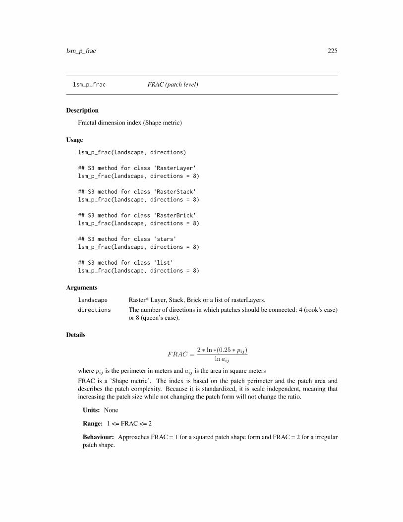
lsm_p_frac 225

lsm_p_frac FRAC (patch level)

Description

Fractal dimension index (Shape metric)

Usage

lsm_p_frac(landscape, directions)

## S3 method for class 'RasterLayer'lsm_p_frac(landscape, directions = 8)

## S3 method for class 'RasterStack'lsm_p_frac(landscape, directions = 8)

## S3 method for class 'RasterBrick'lsm_p_frac(landscape, directions = 8)

## S3 method for class 'stars'lsm_p_frac(landscape, directions = 8)

## S3 method for class 'list'lsm_p_frac(landscape, directions = 8)

Arguments



Details

FRAC =2 ∗ ln ∗(0.25 ∗ pij)

ln aij

where pij is the perimeter in meters and aij is the area in square meters

FRAC is a ’Shape metric’. The index is based on the patch perimeter and the patch area anddescribes the patch complexity. Because it is standardized, it is scale independent, meaning thatincreasing the patch size while not changing the patch form will not change the ratio.

Units: None

Range: 1 <= FRAC <= 2

Behaviour: Approaches FRAC = 1 for a squared patch shape form and FRAC = 2 for a irregularpatch shape.

226 lsm_p_gyrate

Value

tibble

References



See Also

lsm_p_area, lsm_p_perim,lsm_c_frac_mn, lsm_c_frac_sd, lsm_c_frac_cv,lsm_l_frac_mn, lsm_l_frac_sd, lsm_l_frac_cv

Examples

lsm_p_frac(landscape)

lsm_p_gyrate GYRATE (patch level)

Description

Radius of Gyration (Area and edge metric)

Usage

lsm_p_gyrate(landscape, directions)

## S3 method for class 'RasterLayer'lsm_p_gyrate(landscape, directions = 8)

## S3 method for class 'RasterStack'lsm_p_gyrate(landscape, directions = 8)

## S3 method for class 'RasterBrick'lsm_p_gyrate(landscape, directions = 8)

## S3 method for class 'stars'lsm_p_gyrate(landscape, directions = 8)

## S3 method for class 'list'lsm_p_gyrate(landscape, directions = 8)

lsm_p_gyrate 227

Arguments



Details

GY RATE =

z∑r=1

hijrz

where hijr is the distance from each cell to the centroid of the patch and z is the number of cells.

GYRATE is an ’Area and edge metric’. The distance from each cell to the patch centroid is based oncell center-to-cell center distances. The metrics characterises both the patch area and compactness.

Units: Meters

Range: GYRATE >= 0

Behaviour: Approaches GYRATE = 0 if patch is a single cell. Increases, without limit, whenonly one patch is present.

Value

tibble

References



See Also

lsm_c_gyrate_mn, lsm_c_gyrate_sd, lsm_c_gyrate_cv,lsm_l_gyrate_mn, lsm_l_gyrate_sd, lsm_l_gyrate_cv

Examples

lsm_p_gyrate(landscape)

228 lsm_p_ncore

lsm_p_ncore NCORE (patch level)

Description

Number of core areas (Core area metric)

Usage

lsm_p_ncore(landscape, directions, consider_boundary, edge_depth)

## S3 method for class 'RasterLayer'lsm_p_ncore(landscape, directions = 8,consider_boundary = FALSE, edge_depth = 1)

## S3 method for class 'RasterStack'lsm_p_ncore(landscape, directions = 8,consider_boundary = FALSE, edge_depth = 1)

## S3 method for class 'RasterBrick'lsm_p_ncore(landscape, directions = 8,consider_boundary = FALSE, edge_depth = 1)

## S3 method for class 'stars'lsm_p_ncore(landscape, directions = 8,consider_boundary = FALSE, edge_depth = 1)

## S3 method for class 'list'lsm_p_ncore(landscape, directions = 8,consider_boundary = FALSE, edge_depth = 1)

Arguments



consider_boundary


edge_depth Distance (in cells) a cell has the be away from the patch edge to be consideredas core cell#’ @details

NCORE = ncoreij

where ncoreij is the number of disjunct core areas.NCORE is a ’Core area metric’. A cell is defined as core if the cell has noneighbour with a different value than itself (rook’s case). The metric counts the

lsm_p_para 229

disjunct core areas, whereby a core area is a ’patch within the patch’ containingonly core cells. It describes patch area and shape simultaneously (more corearea when the patch is large, however, the shape must allow disjunct core areas).Thereby, a compact shape (e.g. a square) will contain less disjunct core areasthan a more irregular patch.

Units: None

Range: NCORE >= 0

Behaviour: NCORE = 0 when CORE = 0, i.e. every cell in patch is edge.Increases, without limit, as core area increases and patch shape allows disjunctcore areas (i.e. patch shape becomes rather complex).

Value

tibble

References


See Also

lsm_c_dcore_mn, lsm_c_dcore_sd, lsm_c_dcore_cv, lsm_c_ndca,lsm_l_dcore_mn, lsm_l_dcore_sd, lsm_l_dcore_cv, lsm_l_ndca

Examples

lsm_p_ncore(landscape)

lsm_p_para PARA (patch level)

Description

Perimeter-Area ratio (Shape metric)

Usage

lsm_p_para(landscape, directions)

## S3 method for class 'RasterLayer'lsm_p_para(landscape, directions = 8)

## S3 method for class 'RasterStack'lsm_p_para(landscape, directions = 8)

230 lsm_p_para

## S3 method for class 'RasterBrick'lsm_p_para(landscape, directions = 8)

## S3 method for class 'stars'lsm_p_para(landscape, directions = 8)

## S3 method for class 'list'lsm_p_para(landscape, directions = 8)

Arguments



Details

PARA =pijaij

where pij is the perimeter in meters and aij is the area in square meters.

PARA is a ’Shape metric’. It describes the patch complexity in a straightforward way. However,because it is not standarised to a certain shape (e.g. a square), it is not scale independent, meaningthat increasing the patch size while not changing the patch form will change the ratio.

Units: None

Range: PARA > 0

Behaviour: Increases, without limit, as the shape complexity increases.

Value

tibble

References


See Also

lsm_p_area, lsm_p_perim,lsm_c_para_mn, lsm_c_para_sd, lsm_c_para_cv,lsm_l_para_mn, lsm_l_para_sd, lsm_l_para_cv

lsm_p_perim 231

Examples

lsm_p_para(landscape)

lsm_p_perim PERIM (patch level)

Description

Perimeter (Area and edge metric))

Usage

lsm_p_perim(landscape, directions)

## S3 method for class 'RasterLayer'lsm_p_perim(landscape, directions = 8)

## S3 method for class 'RasterStack'lsm_p_perim(landscape, directions = 8)

## S3 method for class 'RasterBrick'lsm_p_perim(landscape, directions = 8)

## S3 method for class 'stars'lsm_p_perim(landscape, directions = 8)

## S3 method for class 'list'lsm_p_perim(landscape, directions = 8)

Arguments



Details

PERIM = pij

where pij is the perimeter in meters.

PERIM is an ’Area and edge metric’. It equals the perimeter of the patch including also the edge tothe landscape boundary. The metric describes patch area (larger perimeter for larger patches), butalso patch shape (large perimeter for irregular shapes).

Units: Meters

232 lsm_p_shape

Range: PERIM > 0

Behaviour: Increases, without limit, as patch size and complexity increases.

Value

tibble

References


Examples

lsm_p_perim(landscape)

lsm_p_shape SHAPE (patch level)

Description

Shape index (Shape metric)

Usage

lsm_p_shape(landscape, directions)

## S3 method for class 'RasterLayer'lsm_p_shape(landscape, directions = 8)

## S3 method for class 'RasterStack'lsm_p_shape(landscape, directions = 8)

## S3 method for class 'RasterBrick'lsm_p_shape(landscape, directions = 8)

## S3 method for class 'stars'lsm_p_shape(landscape, directions = 8)

## S3 method for class 'list'lsm_p_shape(landscape, directions = 8)

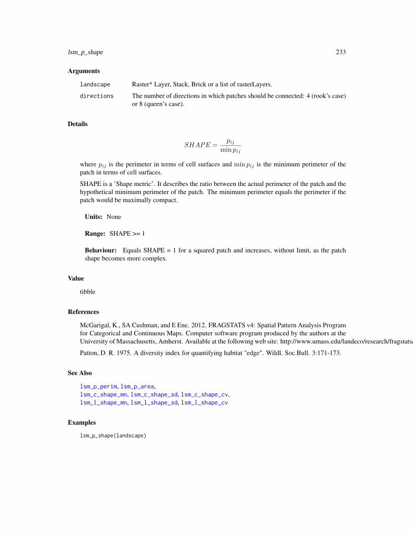
lsm_p_shape 233

Arguments



Details

SHAPE =pij

min pij

where pij is the perimeter in terms of cell surfaces and min pij is the minimum perimeter of thepatch in terms of cell surfaces.

SHAPE is a ’Shape metric’. It describes the ratio between the actual perimeter of the patch and thehypothetical minimum perimeter of the patch. The minimum perimeter equals the perimeter if thepatch would be maximally compact.

Units: None

Range: SHAPE >= 1

Behaviour: Equals SHAPE = 1 for a squared patch and increases, without limit, as the patchshape becomes more complex.

Value

tibble

References



See Also

lsm_p_perim, lsm_p_area,lsm_c_shape_mn, lsm_c_shape_sd, lsm_c_shape_cv,lsm_l_shape_mn, lsm_l_shape_sd, lsm_l_shape_cv

Examples

lsm_p_shape(landscape)

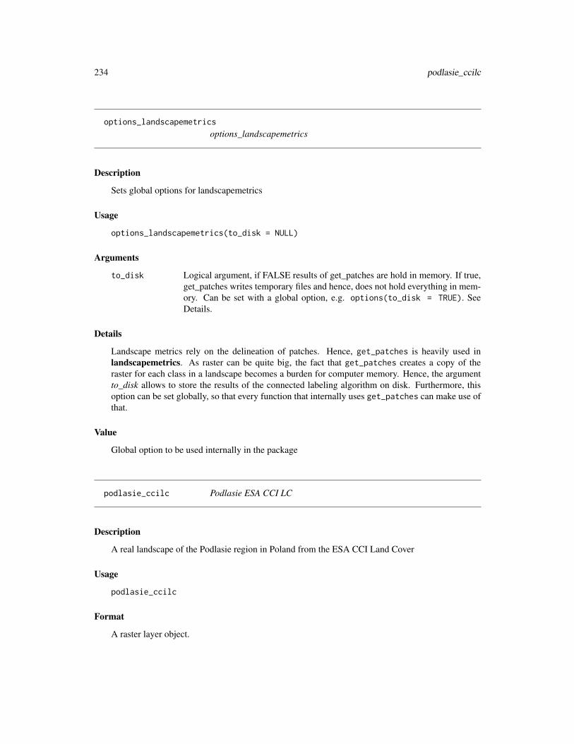
234 podlasie_ccilc

options_landscapemetrics

options_landscapemetrics

Description

Sets global options for landscapemetrics

Usage

options_landscapemetrics(to_disk = NULL)

Arguments

to_disk Logical argument, if FALSE results of get_patches are hold in memory. If true,get_patches writes temporary files and hence, does not hold everything in mem-ory. Can be set with a global option, e.g. options(to_disk = TRUE). SeeDetails.

Details

Landscape metrics rely on the delineation of patches. Hence, get_patches is heavily used inlandscapemetrics. As raster can be quite big, the fact that get_patches creates a copy of theraster for each class in a landscape becomes a burden for computer memory. Hence, the argumentto_disk allows to store the results of the connected labeling algorithm on disk. Furthermore, thisoption can be set globally, so that every function that internally uses get_patches can make use ofthat.

Value

Global option to be used internally in the package

podlasie_ccilc Podlasie ESA CCI LC

Description

A real landscape of the Podlasie region in Poland from the ESA CCI Land Cover

Usage

podlasie_ccilc

Format


sample_lsm 235

Source

http://maps.elie.ucl.ac.be/CCI/viewer/

sample_lsm sample_lsm

Description

Sample metrics

Usage

sample_lsm(landscape, y, shape, size, return_raster, verbose, progress,...)

## S3 method for class 'RasterLayer'sample_lsm(landscape, y, shape = "square", size,return_raster = FALSE, verbose = TRUE, progress = FALSE, ...)

## S3 method for class 'RasterStack'sample_lsm(landscape, y, shape = "square", size,return_raster = FALSE, verbose = TRUE, progress = FALSE, ...)

## S3 method for class 'RasterBrick'sample_lsm(landscape, y, shape = "square", size,return_raster = FALSE, verbose = TRUE, progress = FALSE, ...)

## S3 method for class 'stars'sample_lsm(landscape, y, shape = "square", size,return_raster = FALSE, verbose = TRUE, progress = FALSE, ...)

## S3 method for class 'list'sample_lsm(landscape, y, shape = "square", size,return_raster = FALSE, verbose = TRUE, progress = FALSE, ...)

Arguments

landscape Raster* Layer, Stack, Brick or a list of rasterLayers.y 2-column matrix with coordinates, SpatialPoints, SpatialLines or SpatialPoly-

gons.shape String specifying plot shape. Either "circle" or "square"size Approximated size of sample plot. Equals the radius for circles or half of the

side-length for squares in mapunits. For lines size equals the width of the buffer.return_raster Logical if the clipped raster of the sample plot should be returnedverbose Print warning messages.progress Print progress report.... Arguments passed on to calculate_lsm().

236 sample_lsm

Details

This function samples the selected metrics in a buffer area (sample plot) around sample points,sample lines or within provided SpatialPolygons. The size of the actual sampled landscape can bedifferent to the provided size due to two reasons. Firstly, because clipping raster cells using a circleor a sample plot not directly at a cell center lead to inaccuracies. Secondly, sample plots can exceedthe landscape boundary. Therefore, we report the actual clipped sample plot area relative in relationto the theoretical, maximum sample plot area e.g. a sample plot only half within the landscape willhave a percentage_inside = 50. Please be aware that the output is sligthly different to all otherlsm-function of landscapemetrics.

The metrics can be specified by the arguments what, level, metric, name and/or type (combina-tions of different arguments are possible (e.g. level = "class", type = "aggregation metric").If an argument is not provided, automatically all possibilities are selected. Therefore, to get allavailable metrics, don’t specify any of the above arguments.

Value

tibble

See Also

list_lsmcalculate_lsm

Examples

# use a matrixsample_points <- matrix(c(10, 5, 25, 15, 5, 25), ncol = 2, byrow = TRUE)sample_lsm(landscape, y = sample_points, size = 15, what = "lsm_l_np")

# use sp pointspoints_sp <- sp::SpatialPoints(sample_points)sample_lsm(landscape, y = points_sp, size = 15, what = "lsm_l_np", return_raster = TRUE)

## Not run:# use lines (works only if rgeos is installed)x1 <- c(1, 5, 15, 10)y1 <- c(1, 5, 15, 25)

x2 <- c(10, 25)y2 <- c(5, 5)

sample_lines <- sp::SpatialLines(list(sp::Lines(list(sp::Line(cbind(x1, y1)),sp::Line(cbind(x2, y2))), ID = "a")))sample_lsm(landscape, y = sample_lines, size = 10, what = "lsm_l_np")

# use polygonspoly_1 <- sp::Polygon(cbind(c(2.5, 2.5, 17.5, 17.5),

c(-2.5, 12.5, 12.5, -2.5)))poly_2 <- sp::Polygon(cbind(c(7.5, 7.5, 23.5, 23.5),

c(-7.5, 23.5, 23.5, -7.5)))

show_cores 237

poly_1 <- sp::Polygons(list(poly_1), "p1")poly_2 <- sp::Polygons(list(poly_2), "p2")sample_plots <- sp::SpatialPolygons(list(poly_1, poly_2))

sample_lsm(landscape, y = sample_plots, what = "lsm_l_np")

## End(Not run)

show_cores Show core area

Description

Show core area

Usage

show_cores(landscape, directions, class, labels, nrow, ncol,consider_boundary, edge_depth)

## S3 method for class 'RasterLayer'show_cores(landscape, directions = 8,class = "all", labels = TRUE, nrow = NULL, ncol = NULL,consider_boundary = FALSE, edge_depth = 1)

## S3 method for class 'RasterStack'show_cores(landscape, directions = 8,class = "all", labels = TRUE, nrow = NULL, ncol = NULL,consider_boundary = FALSE, edge_depth = 1)

## S3 method for class 'RasterBrick'show_cores(landscape, directions = 8,class = "all", labels = TRUE, nrow = NULL, ncol = NULL,consider_boundary = FALSE, edge_depth = 1)

## S3 method for class 'stars'show_cores(landscape, directions = 8, class = "all",labels = TRUE, nrow = NULL, ncol = NULL,consider_boundary = FALSE, edge_depth = 1)

## S3 method for class 'list'show_cores(landscape, directions = 8, class = "all",labels = TRUE, nrow = NULL, ncol = NULL,consider_boundary = FALSE, edge_depth = 1)

238 show_correlation

Arguments

landscape Raster object


class How to show the core area: "global" (single map), "all" (every class as facet),or a vector with the specific classes one wants to show (every selected class asfacet).

labels Logical flag indicating whether to print or not to print core labels. boundaryshould be considered as core

nrow, ncol Number of rows and columns for the facet.consider_boundary

Logical if cells that only neighbour the landscape boundary should be consid-ered as core.


Details

The functions plots the core area of patches labeled with the corresponding patch id. The edges arethe grey cells surrounding the patches and are always shown.

Value

ggplot

Examples

# show "global" core areashow_cores(landscape, class = "global", labels = FALSE)

# show the core area of every class as facetshow_cores(landscape, class = "all", labels = FALSE)

# show only the core area of class 1 and 3show_cores(landscape, class = c(1, 3), labels = TRUE)

show_correlation Show correlation

Description

Show correlation

show_lsm 239

Usage

show_correlation(metrics, method = "pearson", diag = TRUE,labels = FALSE, vjust = 0, text_size = 15)

Arguments

metrics Tibble with results of as returned by the landscapemetrics package.

method Type of correlation. See link{cor} for details.

diag If FALSE, values on the diagonal will be NA and not plotted.

labels If TRUE, the correlation value will be added as text.

vjust Will be passed on to ggplot2 as vertical justification of x-axis text.

text_size Text size of the plot.

Details

The functions calculates the correlation between all metrics. In order to calculate correlations, forthe landscape level more than one landscape needs to be present. All input must be structured asreturned by the landscapemetrics package.

Value

ggplot

Examples

metrics <- calculate_lsm(landscape, what = c("patch", "class"))show_correlation(metrics, method = "pearson")

show_lsm Show landscape metrics

Description

Show landscape metrics on patch level printed in their corresponding patch.

Usage

show_lsm(landscape, what, class, directions, consider_boundary, edge_depth,labels, label_lsm, nrow, ncol)

## S3 method for class 'RasterLayer'show_lsm(landscape, what, class = "global",directions = 8, consider_boundary = FALSE, edge_depth = 1,labels = TRUE, label_lsm = FALSE, nrow = NULL, ncol = NULL)

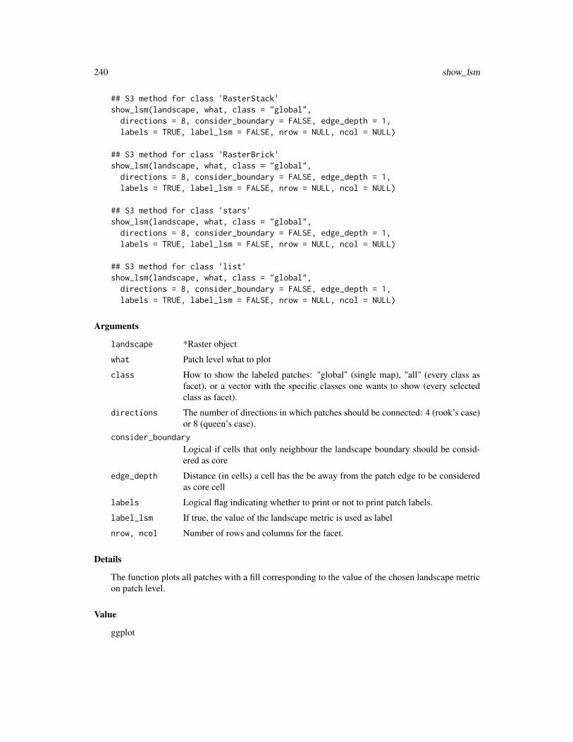
240 show_lsm

## S3 method for class 'RasterStack'show_lsm(landscape, what, class = "global",directions = 8, consider_boundary = FALSE, edge_depth = 1,labels = TRUE, label_lsm = FALSE, nrow = NULL, ncol = NULL)

## S3 method for class 'RasterBrick'show_lsm(landscape, what, class = "global",directions = 8, consider_boundary = FALSE, edge_depth = 1,labels = TRUE, label_lsm = FALSE, nrow = NULL, ncol = NULL)

## S3 method for class 'stars'show_lsm(landscape, what, class = "global",directions = 8, consider_boundary = FALSE, edge_depth = 1,labels = TRUE, label_lsm = FALSE, nrow = NULL, ncol = NULL)

## S3 method for class 'list'show_lsm(landscape, what, class = "global",directions = 8, consider_boundary = FALSE, edge_depth = 1,labels = TRUE, label_lsm = FALSE, nrow = NULL, ncol = NULL)

Arguments

landscape *Raster object

what Patch level what to plot

class How to show the labeled patches: "global" (single map), "all" (every class asfacet), or a vector with the specific classes one wants to show (every selectedclass as facet).


consider_boundary



labels Logical flag indicating whether to print or not to print patch labels.

label_lsm If true, the value of the landscape metric is used as label

nrow, ncol Number of rows and columns for the facet.

Details

The function plots all patches with a fill corresponding to the value of the chosen landscape metricon patch level.

Value

ggplot

show_patches 241

Examples

show_lsm(landscape, what = "lsm_p_area", directions = 4)show_lsm(landscape, what = "lsm_p_shape", class = c(1, 2), label_lsm = TRUE)show_lsm(landscape, what = "lsm_p_circle", class = 3, labels = TRUE)

show_patches Show patches

Description

Show patches

Usage

show_patches(landscape, class, directions, labels, nrow, ncol)

## S3 method for class 'RasterLayer'show_patches(landscape, class = "global",directions = 8, labels = TRUE, nrow = NULL, ncol = NULL)

## S3 method for class 'RasterStack'show_patches(landscape, class = "global",directions = 8, labels = TRUE, nrow = NULL, ncol = NULL)

## S3 method for class 'RasterBrick'show_patches(landscape, class = "global",directions = 8, labels = TRUE, nrow = NULL, ncol = NULL)

## S3 method for class 'stars'show_patches(landscape, class = "global",directions = 8, labels = TRUE, nrow = NULL, ncol = NULL)

## S3 method for class 'list'show_patches(landscape, class = "global",directions = 8, labels = TRUE, nrow = NULL, ncol = NULL)

Arguments

landscape *Raster objectclass How to show the labeled patches: "global" (single map), "all" (every class as

facet), or a vector with the specific classes one wants to show (every selectedclass as facet).


labels Logical flag indicating whether to print or not to print patch labels.nrow, ncol Number of rows and columns for the facet.

242 spatialize_lsm

Details

The functions plots the landscape with the patches labeled with the corresponding patch id.

Value

ggplot

Examples

show_patches(landscape)show_patches(landscape, class = c(1, 2))show_patches(landscape, class = 3, labels = FALSE)

spatialize_lsm spatialize_lsm

Description

Spatialize landscape metric values

Usage

spatialize_lsm(landscape, metric, name, type, what, directions, progress,...)

## S3 method for class 'RasterLayer'spatialize_lsm(landscape, metric = NULL,name = NULL, type = NULL, what = NULL, directions = 8,progress = FALSE, ...)

## S3 method for class 'RasterStack'spatialize_lsm(landscape, metric = NULL,name = NULL, type = NULL, what = NULL, directions = 8,progress = FALSE, ...)

## S3 method for class 'RasterBrick'spatialize_lsm(landscape, metric = NULL,name = NULL, type = NULL, what = NULL, directions = 8,progress = FALSE, ...)

## S3 method for class 'stars'spatialize_lsm(landscape, metric = NULL, name = NULL,type = NULL, what = NULL, directions = 8, progress = FALSE, ...)

## S3 method for class 'list'spatialize_lsm(landscape, metric = NULL, name = NULL,type = NULL, what = NULL, directions = 8, progress = FALSE, ...)

window_lsm 243

Arguments








... Arguments passed on to calculate_lsm().

Details

The functions returns a nested list with RasterLayers. The first level contains each input layer(only one element if RasterLayer was provided). The second level contains a RasterLayer foreach selected metric (see list_lsm for details) where each cell has the landscape metric value ofthe patch it belongs to. Only patch level metrics are allowed.

Value

list

See Also

list_lsmshow_lsm

Examples

spatialize_lsm(landscape, what = "lsm_p_area")

window_lsm window_lsm

Description

Moving window

244 window_lsm

Usage

window_lsm(landscape, window, metric, name, type, what, progress, ...)

## S3 method for class 'RasterLayer'window_lsm(landscape, window, metric = NULL,name = NULL, type = NULL, what = NULL, progress = FALSE, ...)

## S3 method for class 'RasterStack'window_lsm(landscape, window, metric = NULL,name = NULL, type = NULL, what = NULL, progress = FALSE, ...)

## S3 method for class 'RasterBrick'window_lsm(landscape, window, metric = NULL,name = NULL, type = NULL, what = NULL, progress = FALSE, ...)

## S3 method for class 'stars'window_lsm(landscape, window, metric = NULL,name = NULL, type = NULL, what = NULL, progress = FALSE, ...)

## S3 method for class 'list'window_lsm(landscape, window, metric = NULL,name = NULL, type = NULL, what = NULL, progress = FALSE, ...)

Arguments


window matrix






... Arguments passed on to calculate_lsm().

Details

The function calculates for each focal cell the selected landscape metrics (currently only landscapelevel metrics are allowed) for a local neighbourhood. The neighbourhood can be specified usinga matrix. For more details, see ?raster::focal(). The result will be a RasterLayer in whicheach focal cell includes the value of its neighbourhood and thereby allows to show gradients andvariability in the landscape (Hagen-Zanker 2016). To be type stable, the acutally result is always anested list (first level for RasterStack layers, second level for selected landscape metrics).

Value

list

window_lsm 245

References

Fletcher, R., Fortin, M.-J. 2018. Spatial Ecology and Conservation Modeling: Applications with R.Springer International Publishing. 523 pages

Hagen-Zanker, A. (2016). A computational framework for generalized moving windows and itsapplication to landscape pattern analysis. International journal of applied earth observation andgeoinformation, 44, 205-216.

McGarigal, K., Cushman, S.A., and Ene E. 2012. FRAGSTATS v4: Spatial Pattern Analysis Pro-gram for Categorical and Continuous Maps. Computer software program produced by the au-thors at the University of Massachusetts, Amherst. Available at the following website: http://www.umass.edu/landeco/research/fragstats/fragstats.html

See Also

list_lsmcalculate_lsmfocal

Examples

## Not run:window <- matrix(1, nrow = 5,ncol = 5)window_lsm(landscape, window = window, what = c("lsm_l_pr", "lsm_l_joinent"))window_lsm(landscape_stack, window = window, what = c("lsm_l_pr", "lsm_l_joinent"))

## End(Not run)

http://www.umass.edu/landeco/research/fragstats/fragstats.html

http://www.umass.edu/landeco/research/fragstats/fragstats.html

Index

∗Topic datasetsaugusta_nlcd, 6fragstats_class_augusta_nlcd, 12fragstats_class_landscape, 12fragstats_class_podlasie, 13fragstats_landscape_augusta_nlcd,

13fragstats_landscape_landscape, 14fragstats_landscape_podlasie, 14fragstats_patch_augusta_nlcd, 15fragstats_patch_landscape, 15fragstats_patch_podlasie, 16landscape, 25lsm_abbreviations_names, 27podlasie_ccilc, 234

augusta_nlcd, 6

calculate_lsm, 6, 11, 236, 245check_landscape, 9cv, 30, 36, 54, 63, 71, 76, 80, 83, 97, 106, 117,

122, 141, 148, 156, 162, 167, 170,188, 199

extract_lsm, 10

focal, 245fragstats_class_augusta_nlcd, 12fragstats_class_landscape, 12fragstats_class_podlasie, 13fragstats_landscape_augusta_nlcd, 13fragstats_landscape_landscape, 14fragstats_landscape_podlasie, 14fragstats_patch_augusta_nlcd, 15fragstats_patch_landscape, 15fragstats_patch_podlasie, 16

get_adjacencies, 16get_boundaries, 18get_circumscribingcircle, 19get_nearestneighbour, 20

get_patches, 20, 21, 21get_unique_values, 23

landscape, 25landscapemetrics, 25landscapemetrics-package

(landscapemetrics), 25list_lsm, 8, 26, 236, 243, 245lsm_abbreviations_names, 27lsm_c_ai, 28, 116lsm_c_area_cv, 29, 32, 33, 117, 119, 120, 216lsm_c_area_mn, 30, 31, 33, 117, 119, 120, 216lsm_c_area_sd, 30, 32, 32, 117, 119, 120, 216lsm_c_ca, 31, 34, 105, 211, 216lsm_c_cai_cv, 35, 38, 40, 122, 124, 125, 218lsm_c_cai_mn, 36, 37, 40, 122, 125, 218lsm_c_cai_sd, 36, 38, 38, 122, 124, 125, 218lsm_c_circle_cv, 40, 43, 44, 127, 128, 130,

219lsm_c_circle_mn, 41, 42, 44, 127, 128, 130,

219lsm_c_circle_sd, 41, 43, 43, 127, 128, 130,

219lsm_c_clumpy, 45lsm_c_cohesion, 46lsm_c_contig_cv, 48, 49, 51, 52, 136, 138,

139, 221lsm_c_contig_mn, 49, 49, 52, 136, 138, 139,

221lsm_c_contig_sd, 51, 51, 136, 138, 139, 221lsm_c_core_cv, 53, 56, 57, 141, 143, 144, 223lsm_c_core_mn, 54, 54, 57, 141, 143, 144, 223lsm_c_core_sd, 54, 56, 56, 141, 143, 144, 223lsm_c_cpland, 58, 218lsm_c_dcad, 59, 146lsm_c_dcore_cv, 61, 64, 66, 148, 150, 151,

229lsm_c_dcore_mn, 63, 63, 66, 148, 150, 151,

229

246

INDEX 247

lsm_c_dcore_sd, 63, 64, 65, 148, 150, 151,229

lsm_c_division, 66, 89, 153, 177lsm_c_division.stars (lsm_c_area_sd), 32lsm_c_ed, 68, 154lsm_c_enn_cv, 70, 73, 74, 156, 158, 159, 224lsm_c_enn_mn, 71, 71, 74, 156, 158, 159, 224lsm_c_enn_sd, 71, 73, 73, 156, 158, 159, 224lsm_c_frac_cv, 75, 77, 79, 162, 164, 165, 226lsm_c_frac_mn, 76, 76, 79, 162, 164, 165, 226lsm_c_frac_sd, 76, 77, 78, 162, 164, 165, 226lsm_c_gyrate_cv, 79, 82, 83, 167, 168, 170,

227lsm_c_gyrate_mn, 80, 81, 83, 167, 168, 170,

227lsm_c_gyrate_sd, 80, 82, 82, 167, 168, 170,

227lsm_c_iji, 84, 171lsm_c_lpi, 85, 174lsm_c_lsi, 87, 176lsm_c_mesh, 67, 88, 152, 177lsm_c_ndca, 61, 90, 146, 183, 229lsm_c_nlsi, 91lsm_c_np, 93, 101, 102, 185, 192lsm_c_pafrac, 94, 186lsm_c_para_cv, 96, 99, 100, 188, 189, 191,

230lsm_c_para_mn, 97, 98, 100, 188, 189, 191,

230lsm_c_para_sd, 97, 99, 99, 188, 189, 191, 230lsm_c_pd, 101, 192lsm_c_pladj, 102lsm_c_pland, 103, 204, 205, 207, 208lsm_c_shape_cv, 105, 108, 109, 199, 201,

202, 233lsm_c_shape_mn, 106, 107, 109, 199, 201,

202, 233lsm_c_shape_sd, 106, 108, 108, 199, 201,

202, 233lsm_c_split, 110, 210lsm_c_tca, 91, 111, 183, 213, 223lsm_c_te, 69, 113lsm_l_ai, 29, 114lsm_l_area_cv, 30, 32, 33, 116, 119, 120, 216lsm_l_area_mn, 30, 32, 33, 117, 117, 120, 216lsm_l_area_sd, 30, 32, 33, 117, 119, 119, 216lsm_l_cai_cv, 36, 38, 40, 120, 124, 125, 218lsm_l_cai_mn, 36, 38, 40, 122, 122, 125, 218

lsm_l_cai_sd, 36, 38, 40, 122, 124, 124, 218lsm_l_circle_cv, 41, 43, 44, 126, 128, 130,

219lsm_l_circle_mn, 41, 43, 44, 127, 127, 130,

219lsm_l_circle_sd, 41, 43, 44, 127, 128, 129,

219lsm_l_cohesion, 47, 130, 131lsm_l_condent, 132, 161, 173, 182lsm_l_contag, 133lsm_l_contig_cv, 49, 51, 52, 135, 138, 139,

221lsm_l_contig_mn, 49, 51, 52, 136, 136, 139,

221lsm_l_contig_sd, 49, 51, 52, 136, 138, 138,

221lsm_l_core_cv, 54, 56, 57, 140, 143, 144, 223lsm_l_core_mn, 54, 56, 57, 141, 141, 144, 223lsm_l_core_sd, 54, 56, 57, 141, 143, 143, 223lsm_l_dcad, 61, 145lsm_l_dcore_cv, 63, 64, 66, 146, 150, 151,

229lsm_l_dcore_mn, 63, 64, 66, 148, 148, 151,

229lsm_l_dcore_sd, 63, 64, 66, 148, 150, 150,

229lsm_l_division, 68, 152lsm_l_ed, 69, 153lsm_l_enn_cv, 71, 73, 74, 155, 158, 159, 224lsm_l_enn_mn, 71, 73, 74, 156, 156, 159, 224lsm_l_enn_sd, 71, 73, 74, 156, 158, 158, 224lsm_l_ent, 133, 160, 173, 182lsm_l_frac_cv, 76, 77, 79, 161, 164, 165, 226lsm_l_frac_mn, 76, 77, 79, 162, 163, 165, 226lsm_l_frac_sd, 76, 77, 79, 162, 164, 164, 226lsm_l_gyrate_cv, 80, 82, 83, 166, 168, 170,

227lsm_l_gyrate_mn, 80, 82, 83, 167, 167, 170,

227lsm_l_gyrate_sd, 80, 82, 83, 167, 168, 169,

227lsm_l_iji, 85, 170lsm_l_joinent, 133, 161, 172, 181, 182lsm_l_lpi, 86, 173lsm_l_lsi, 88, 174lsm_l_mesh, 89, 176lsm_l_msidi, 178lsm_l_msiei, 179

248 INDEX

lsm_l_mutinf, 133, 161, 173, 181lsm_l_ndca, 91, 182, 229lsm_l_np, 94, 184, 192lsm_l_pafrac, 96, 185lsm_l_para_cv, 97, 99, 100, 187, 189, 191,

230lsm_l_para_mn, 97, 99, 100, 188, 188, 191,

230lsm_l_para_sd, 97, 99, 100, 188, 189, 190,

230lsm_l_pd, 102, 191lsm_l_pladj, 193lsm_l_pr, 194, 196, 205, 207, 208lsm_l_prd, 195lsm_l_rpr, 197lsm_l_shape_cv, 106, 108, 109, 198, 201,

202, 233lsm_l_shape_mn, 106, 108, 109, 199, 200,

202, 233lsm_l_shape_sd, 106, 108, 109, 199, 201,

201, 233lsm_l_shdi, 203, 206lsm_l_shei, 204lsm_l_sidi, 179, 206lsm_l_siei, 180, 207lsm_l_split, 111, 209lsm_l_ta, 35, 59, 61, 68, 69, 86, 89, 102, 105,

111, 118, 146, 153, 154, 174, 177,192, 210, 210, 216

lsm_l_tca, 112, 212, 223lsm_l_te, 114, 154, 213, 215lsm_p_area, 30, 32, 33, 35, 47, 68, 86, 89, 96,

111, 117, 119, 120, 131, 153, 174,177, 186, 210, 211, 215, 218, 219,226, 230, 233

lsm_p_cai, 36, 38, 40, 122, 124, 125, 216lsm_p_circle, 41, 43, 44, 127, 128, 130, 218lsm_p_contig, 49, 51, 52, 136, 138, 139, 220lsm_p_core, 54, 56, 57, 59, 112, 141, 143,

144, 213, 218, 221lsm_p_enn, 71, 73, 74, 156, 158, 159, 223lsm_p_frac, 76, 77, 79, 162, 164, 165, 225lsm_p_gyrate, 80, 82, 83, 167, 168, 170, 226lsm_p_ncore, 63, 64, 66, 91, 148, 150, 151,

183, 228lsm_p_para, 97, 99, 100, 188, 189, 191, 229lsm_p_perim, 47, 96, 114, 131, 186, 215, 226,

230, 231, 233

lsm_p_shape, 88, 93, 106, 108, 109, 176, 199,201, 202, 232

mean, 32, 38, 41, 43, 44, 56, 64, 73, 77, 82, 99,108, 119, 124, 127, 128, 130, 143,150, 158, 164, 168, 189, 201

options_landscapemetrics, 234

podlasie_ccilc, 234

sample_lsm, 235sd, 33, 40, 57, 66, 74, 79, 100, 109, 120, 125,

144, 151, 159, 165, 191, 202show_cores, 237show_correlation, 238show_lsm, 239, 243show_patches, 241spatialize_lsm, 242sum, 35, 211

window_lsm, 243

package ‘landscapemetrics’ - cran.r-project.org · 6 calculate_lsm augusta_nlcd augusta nlcd...

Documents