Quantum state engineering in hybrid open quantum systems

Chaitanya Joshi,1, ∗ Jonas Larson,2 and Timothy P. Spiller1

1Department of Physics and York Centre for Quantum Technologies,University of York, Heslington, York, YO10 5DD, UK

2Department of Physics, Stockholm University, Albanova physics center, Se-106 91 Stockholm, Sweden(Dated: March 30, 2016)

We investigate a possibility to generate non-classical states in light-matter coupled noisy quan-tum systems, namely the anisotropic Rabi and Dicke models. In these hybrid quantum systems acompeting influence of coherent internal dynamics and environment induced dissipation drives thesystem into non-equilibrium steady states (NESSs). Explicitly, for the anisotropic Rabi model thesteady state is given by an incoherent mixture of two states of opposite parities, but as each paritystate displays light-matter entanglement we also find that the full state is entangled. Furthermore,as a natural extension of the anisotropic Rabi model to an infinite spin subsystem, we next exploredthe NESS of the anisotropic Dicke model. The NESS of this linearized Dicke model is also an in-separable state of light and matter. With an aim to enrich the dynamics beyond the sustainableentanglement found for the NESS of these hybrid quantum systems, we also propose to combinean all-optical feedback strategy for quantum state protection and for establishing quantum controlin these systems. Our present work further elucidates the relevance of such hybrid open quantumsystems for potential applications in quantum architectures.

PACS numbers: 42.50.Pq, 42.50.Ct, 03.67.Bg, 03.65.Yz

I. INTRODUCTION

Light-matter coupled quantum systems are now seenas novel composite systems for the exploration of vari-ous tasks in quantum computation and information pro-cessing, as well as for testing foundations of quantumphysics [1–3]. These hybrid systems promise to com-bine disparate quantum degrees of freedom in construct-ing scalable quantum architectures [1, 4]. In particular,the idea is to take ‘the best of two worlds’: matter pro-vides good candidates for storage of quantum informa-tion, while light (photons) are superior when it comesto transmitting or sending quantum information, withinteractions between these provide processing. For ex-ample, photons can be sent between different parties inorder to create entanglement over macroscopic distances.However, physical quantum systems, in this case espe-cially the light part, invariably also couple to their ex-ternal environments [5, 6]. It is commonly argued thatnon-classical states, including entangled states, are ex-tremely sensitive to noise and dissipation. For exam-ple, environment induced decoherence tends to reducequantum-coherent superpositions to incoherent mixtures[7]. Quantum state engineering strategies have thereforetaken a center stage in salvaging quantum coherence inhybrid quantum systems [1, 8]. It is clear that for usingphotons as information carriers between different mat-ter subsystems, sustainable entanglement between lightand matter is a necessity, i.e. such quantum correlationsshould survive any realistic decoherence/noise affectingthe photons.

∗Electronic address: chaitanya.joshi@york.ac.uk

In a somewhat parallel approach, noisy coupled quan-tum systems have been proposed as exciting avenues forcontrolled generation of multi-partite entangled states[9]. The interplay between coherent and incoherent dy-namics in interacting multi-partite open quantum sys-tems can result in the generation of steady states whichexhibit exotic quantum character [10, 11]. To take a par-ticular example relevant for this work, for open opticalsystems the dynamics can often be well described by aLindblad type master equation

˙ρ = −i[HS, ρ] + γLAρ, (1)

where ρ is the system’s state, HS the system Hamilto-nian, and LAρ is the Lindblad super operator render-

ing the effects of the reservoir on the system (A is the

so called quantum jump operator, and we note that HS

may be modified from the closed system Hamiltonian dueto the interaction with the environment). The steady

state is solved by letting i[HS, ρss] − γLAρss = 0. It fol-

lows that if ρss is a dark state, i.e. LAρss = 0, then

ρss must also commute with HS, e.g. being an eigen-state of the Hamiltonian. However, this is not the onlypossibility for having a steady state; both contributionsmight be non-zero but also exactly cancel each other.This would mean that the unitary evolution ‘balances’the non-unitary evolution. For infinite systems, this in-terplay may result in non-equilibrium phase transitionsbetween phases supported either by the first or the sec-ond term in Eq.(1) [10, 11]. That is to say that ρss

changes qualitatively and shows non-analytic propertiesat some critical γc. For finite systems, on the otherhand, such a transition is smooth/analytic, but never-theless for the intermediate stages between the two ex-tremes non-classical states may persist. In this work

arX

iv:1

509.

0359

9v2

[qu

ant-

ph]

29

Mar

201

6

2

we explore this scenario and examine the possibility ofgenerating non-classical states in two open quantum sys-tems that have served as work horses in quantum opticsfor more than half a century, namely the Rabi [12] (ornon-Rotating-Wave-Approximation (non-RWA) Jaynes-Cummings model [13]) and the Dicke model [14]. In away, in our study these two models are at the two ex-tremes of the quantum spectrum; the Rabi model whichcouples a single spin-1/2 particle to a boson or photonmode lives in the deep quantum regime, while what weterm the Dicke model considers instead a particle withan infinite large spin S (almost classical) coupled to theboson mode. As already mentioned, the main sourceof decoherence is very often photon absorption and wethereby consider a Lindblad term with A = a being thephoton annihilation operator. This photon loss mecha-nism aims at emptying the boson mode (the only darkstate is the vacuum). However, for a large light-mattercoupling in the Hamiltonian even the ground state (inthe absence of environmental coupling) becomes a ‘highlyexcited’ (from the perspective of photon number) state,and so the two dynamical contributions in the evolutionof the hybrid system must be balanced in order to sup-port a NESS. We will demonstrate that as a result of thiscompetition between unitary and non-unitary evolution,for both models a NESS exists that possess non-classicalfeatures in terms of light-matter entanglement. Further-more, especially for the Rabi model this NESS reflectsthe well known parity symmetry of the original Hamil-tonian; the NESS consists of an incoherent mixture ofdifferent parity states.

In the second half of the paper we explore possibilitiesto systematically enrich and enhance the non-classicalproperties of the NESS. More precisely, although envi-ronment induced dissipation potentially can be tailoredto achieve desired quantum states [15], establishing quan-tum control over various dissipation channels is also animportant benchmark toward realizing a useful quantumarchitecture [16]. Thus, it is desirable to construct quan-tum control schemes for hybrid quantum processors if, forinstance, one is interested in initial quantum state preser-vation [17]. Along these lines we will use an all-opticalcoherent feedback strategy [18–20] to achieve quantumstate preservation. It is important to appreciate thatsuch a scheme is different from just tailoring the dissipa-tion channels as it involves active feedback to the system.As outlined in Refs. [18, 19], under the assumption thatthe time-delay introduced by the feedback loop is negli-gible it is indeed possible to establish a complete controlover the dissipative dynamics. Going beyond such ideal-ized sudden feedback control, we will conclude by brieflycommenting on the prospects of our scheme by combin-ing it with a time-delayed feedback control scheme aspreviously studied both in the classical [21] and quan-tum domains [22, 23].

The paper is organized as follows. In Sec.II we intro-duce our first physical model describing the interactionbetween a quantized bosonic mode and a single two-level

system. We explore the general structure of the NESS ρss

(being of an interesting form) and extract the sustainableentanglement between the two subsystems. The follow-ing Sec.III addresses the question whether non-classicalfeatures survive in the ‘classical limit’ in which the two-level system is turned into an infinite one i.e. identifyingthe linearized Dicke model. And indeed, entanglement issustained also in this case. Having discussed these twomodel examples, in Sec. IV we combine a coherent all-optical feedback scheme for quantum state protection inopen quantum systems. While entanglement is sustain-able in the original open systems, the feedback schemeallows for increasing the desired properties. Finally, weconclude the paper with a short discussion in Sec. V.

II. MODEL A - ANISOTROPIC RABI MODEL

The quantum Rabi model describes the interaction be-tween a quantized bosonic field and the simplest quan-tum mechanical model, a single two-level system or qubit[12]. Despite its simplicity, the quantum Rabi model hadeluded an exact solution for many decades and it was onlyrecently that an analytical solution was obtained [24],with continuing debate as to the completeness of this so-lution and the existence of other possible solutions [25].Nonetheless, over the years the quantum Rabi model hasturned out to be an ubiquitous physical model and hasfound applications in understanding a wide variety ofphysical systems, including trapped ions, superconduct-ing qubits, optical and microwave cavity QED, circuitQED, among others [26]. In some cases the two-levelsystem may be an exact description of the matter partof the hybrid system (when it is indeed a spin-1/2 par-ticle), but in many cases the two-level description is anapproximation of a more complicated matter sub-system.

In its most simplified form the quantum Rabi modeltakes the form (with ~=1 and neglecting the vacuum en-ergy of the boson mode)

HRM = ωa†a+Ω

2σz + λ(a† + a)(σ+ + σ−). (2)

Here, a and a† are the annihilation and creation operatorsfor the bosonic field of frequency ω, σ± = (σx ± iσy)/2with σx,y,z the Pauli matrices for the two-level system, Ωis the energy level splitting between the two levels, andthe coupling strength between the bosonic mode and thetwo-level system is represented as λ (≥ 0). Through-out we will use dimensionless parameters such that wescale all frequencies by ω and time by ω−1. Neverthe-less, we keep ω in all expressions in order to keep trackof all terms and instead always use ω = 1 in any calcu-lations. The counter-rotating terms in the Hamiltonian(2), a†σ+ and σ−a, do not conserve the excitation num-ber. However, if the coupling λ ω,Ω, these counter-rotating terms can be dropped from the Hamiltonian(2) under the so-called Rotating Wave Approximation(RWA) [13, 28]. Simplifying the Hamiltonian (2) under

3

the RWA results in the widely studied Jaynes-Cummingsmodel which can be straightforwardly solved [13, 30].As evident through several standard cavity-QED exper-iments, the atom-field coupling λ is normally orders ofmagnitude smaller than the bare transition frequenciesω,Ω, and this makes the RWA a valid approximationto simplify the quantum Rabi model [3]. The straight-forward solvable nature of the Jaynes-Cummings modelresults from the presence of a continuous U(1) symme-

try; the total number of excitations N = a†a + 12 σz is

preserved. This should be contrasted with the discreteZ2 parity symmetry of the Rabi model characterized bythe unitary UZ2 = exp

[i(a†a+ σ+σ−

)π]. The action

of UZ2 is to flip the signs of a, a†, σx,y while leaving σzinvariant. Thus, the Rabi model has a lower symmetrythan the Jaynes-Cummings model, which naturally is thereason why finding an exact Rabi solution is very hard.

The RWA simplified quantum Rabi model is undoubt-edly one of the most celebrated models in quantum opticsand has received well deserved attention [30–32]. How-ever, there has been a recent surge of interest in exploringhybrid quantum systems in the so-called “ultra-strong”coupling regime [33]. In this ultra-strong coupling regimethe atom-field coupling strength λ can approach a non-negligible fraction of the bare transition frequencies ω,Ω,thereby making the Jaynes-Cummings model a non-validapproximation for the quantum Rabi model [34]. Fromthe discussion of the introduction, it should be clearthat in order to generate large steady state entanglementthe coupling λ should be made as large as possible (al-lowed by other approximations like the two-level approx-imation). As λ >

√ωΩ the ground state of the Rabi

model undergoes a qualitative change [32, 35] where thefield builds up a large non-zero photon number. In theDicke model this marks the normal-superradiant phasetransition [36]. This extremely large λ regime has beentermed the “deep strong” coupling regime [37]. Thus,as the ultra-strong coupling regime has recently beenrealized in certain (non-driven) circuit QED architec-tures [33] (λ ∼ ω/10), we would like to explore the quan-tum Rabi model further, into the deep strong couplingregime where the coupling parameter λ ∼ ω,Ω. It isstill unclear whether or not a non-driven system couldattain such couplings [38]. Equally important, in thisdeep strong coupling regime the no-go theorem tells usthat the ‘self-energy’ of the field cannot be neglected andby including such a term the passing to a large photonpopulated ground state will not occur [41]. Therefore,to overcome such hindrances we choose to work with aneffective realization of the quantum Rabi model with suit-ably engineered Raman driving [15, 28, 29]. Furthermore,as such driven models may derive more generalized ver-sions of HRM, we will work with the anisotropic Rabimodel (ARM) [42]

HARM = ωa†a+Ω

2σz+λ1

(a†σ−+ σ+a

)+λ2

(a†σ++ σ−a

).

(3)

The possibility to realize the above ARM and also totune ω,Ω, λ1, λ2 relative to each other derives from thefact that amplitude of the Raman drive effectively de-termines the coupling parameters [15, 28, 29]. With thismodel it is also easy to extract the importance of thecounter rotating terms neglected in the RWA. In par-ticular, the above Hamiltonian reduces to the Jaynes-Cummings model when λ2 = 0, and to the quantumRabi-model when λ1 = λ2 = λ. One important observa-tion is that the Z2 parity symmetry is preserved for theanisotropic Rabi model which naturally implies that theeigenstates can be assigned an even or odd parity, i.e.simultaneous eigenstates of UZ2 with ±1 eigenvalues. Inpassing we may note that recently, the anisotropic Rabimodel was also termed the U(1)/Z2 Rabi model as it in-cludes both the Jaynes-Cummings and Rabi models aslimiting cases [43]. A general state (not an eigenstate)with even(+)/odd(−) parity takes the respective forms

|Ψ+〉 =∑n

(c↑n|2n+ 1〉| ↑〉+ c↓n|2n〉| ↓〉

),

|Ψ−〉 =∑n

(d↑n|2n〉| ↑〉+ d↓n|2n+ 1〉| ↓〉

),

(4)

where the first ket state |n〉 represents the boson Fockstate and the second |↑〉/|↓〉 the “up/down” eigenstateof the Pauli z matrix. Naturally, the coefficients c↑,↓nand d↑,↓n will depend on the system parameters and, dueto the simplicity of the Rabi model, they can in princi-ple be accurately obtained by numerical diagonalizationof (3). Let us give one more comment related to the

symmetries of HARM. To make this comment clear weassume that the boson mode is only weakly populatedsuch that we can truncate it to contain only the vac-uum and the first Fock state. In this case we relabelthe creation/annihilation operators with τ+/τ− respec-tively. In this truncated space we can define effectivePauli operators τ+ = (τx + iτy)/2, τ− = (τx − iτy)/2,and τz = 2τ+τ− − 1. Within this approximation andformulation we rewrite the Hamiltonian as (up to a con-stant)

HARM = ωτz+Ω

2σz+

λ1 + λ2

2τxσx++

λ1 − λ2

2τyσy. (5)

Expressed in this form we can identify the Jaynes-Cummings model (λ2 = 0) with the two site HeisenbergXX model and the anti-Jaynes-Cummings model [44](λ1 = 0) also with the XX model but with one cou-pling supporting ferro- and the other anti-ferromagneticorder. Similarly, the Rabi model (λ1 = λ2) can be identi-fied with the two site transverse Ising model, and finallythe ARM (λ1 6= λ2) with the two site Heisenberg XYmodel. Naturally, the character of the couplings are notjust limited to the above approximation where the bosonHilbert space has been truncated to two states, but holdsalso for the original Hamiltonian. We cannot talk aboutphase transitions in these finite size models (contrary to

4

the Dicke model), but nevertheless the types of couplingshare great similarities with these spin systems which allare critical in the thermodynamic limit [45]. We notethat the Dicke phase transition is within the Ising modeluniversality class. Even though we cannot properly takea thermodynamic limit of the Rabi model, it was shownthat typical features (non-analyticity and vanishing or-der parameter in one phase) of a phase transition canalso be achieved in the Rabi model by letting Ω/ω →∞.Not surprisingly, here one also finds universal Ising be-havior [46].

In [15] an effective optical realization of the Hamilto-nian (3) based on multi-level atoms and cavity-mediatedRaman transitions has been presented. Most recentlythis scheme was also experimentally demonstrated, andimportantly the deep strong coupling regime of the Dickemodel was reached [47]. A many-body generalization ofthe Hamiltonian (3) has also been recently considered, toexplore the non-equilibrium phase diagram of the dissi-pative Rabi-Hubbard model [48]. We will not enter intothe details of a physical realization of the Hamiltonian(3), but will refer the reader to a comprehensive analysisperformed in [15].

Following [15], damping of the field mode is the dom-inant source of dissipation and so we will approximateby taking it as the only dissipation channel in the openversion of the ARM (3). This assumption is particularlyvalid for the scheme outlined in [15] where the metastablelow lying energy doublet of a Raman driven four levelatom can act as a qubit in the ARM (3). Under the Born-Markov and secular approximations [5, 6], we model theevolution of the joint atom-field density operator ρ bythe master equation

˙ρ = −i[HARM, ρ] + γLaρ, (6)

where γ is the damping rate of the field and Lxρ =2xρx† − x†xρ − ρx†x is the Lindblad super operator. Itis worth noting that in writing the above master equa-tion we have assumed that the cavity damping is inde-pendent of the inter-mode coupling strengths λ1 and λ2.The form of the master equation (6) can only arise outof an original time-dependent (driven) Hamiltonian. Inthe approach outlined in [15] the coupling Hamiltonian(3) is written in the frame of an external drive, impartingit a non-equilibrium character. For a time-independentsystem coupled to an external bath, it is required thatthe steady state will obey the principles of equilibriumstatistical mechanics [49]. No such restriction is requiredon the dynamics arising out of a implicit time-dependentHamiltonian. Naturally, this is crucial in our study, aswe reach steady states that are different from a thermalequilibrium state. We thereby can conclude that evenif deep strong coupling regime could be reached withoutexternal pumping such a model would be conceptuallydifferent from the present one as the Lindblad jump op-erators would be different [50].

In order to analyze the particular structure of thesteady states ρss we numerically solve the master equa-

tion (6) and explore the resulting NESS. The steady stateis found by integrating the equation for long times, forvarious initial states, and checking for convergence of thesolution. According to the above discussion, a steadystate cannot be a dark state in this case since we knowthat the dark state is the vacuum which in return is notan eigenstate of the Hamiltonian. We further know thatsince the system is driven, the NESS should be differentfrom the system ground state which becomes the steadystate when the system is coupled to a zero temperaturebath [50]. However, less clear is whether the steady stateis unique. This could, in principle, be checked by diag-onalizing the master equation, but here we only remarkthat our numerical simulations, for given parameters andfor different initial states, all relax to steady states of aspecific form.

Through numerical evaluation of the master equation(6) we arrive at the atom-field NESS density matrix ρss

and find it to have an approximate structure when order-ing the elements in a specific way. In a three-excitationmanifold, for instance, ρss can be explicitly expressed as

ρss =

〈0 ↑ | 〈0 ↓ | 〈1 ↑ | 〈1 ↓ | 〈2 ↑ | 〈2 ↓ | 〈3 ↑ | 〈3 ↓ ||0 ↑〉 × × × ×|0 ↓〉 × × × ×|1 ↑〉 × × × ×|1 ↓〉 × × × ×|2 ↑〉 × × × ×|2 ↓〉 × × × ×|3 ↑〉 × × × ×|3 ↓〉 × × × ×

,

(7)where the crosses mark the non-vanishing elements. Theabove structure tells us that the overlap between thestates of opposite parities in the steady state density ma-trix ρss is identically zero.

We can give a qualitative argument which allows theabove structure of the density matrix ρss. The Lind-blad super operator is obviously invariant under the ac-tion of UZ2

; Laρ = LUZ2aU−1

Z2

ρ. As discussed in detail

above, the ARM (3) is also invariant under the action of

parity operator UZ2 . Combining these two observationsmight tempt us to believe that the entire Lindblad mas-ter equation (6) is also symmetric under UZ2 . However,it is important to recognize that for open quantum sys-tems a symmetry does not necessarily imply a conservedquantity [51]. Thus, in general we do not have such athing as Noether’s theorem for open quantum systems.The numerically obtained steady state density matrix ρss

confirms this conjecture. In other words, the parity con-servation of the original ARM (3) is broken under theevolution described by the Lindblad master equation (6).

The steady state density matrix ρss (7) can also beexpressed in a closed form as

ρss = cos2 θ|Ψ+〉〈Ψ+|+ sin2 θ|Ψ−〉〈Ψ−|, (8)

with the parity states (4), and θ is some constant deter-mined by the system parameters. Thus, any coherencebetween the states of opposite parities is lost and thesteady state is an incoherent mixture of these. Neverthe-less, in the steady state quantum coherence can survive

5

among the states with definite parity. The parameter θis in general not 0 nor π, meaning that parity is not aconserved quantity under evolution of (6); for example,an initial state with a definite parity will typically alsoend up in an incoherent mixture of the two parity states|Ψ±〉. In the language of ‘pointer states’ [52], the statesrobust to the present decoherence are those with certainparity.

In support of the structure of the steady state den-sity matrix (8) we argue that it is due to a symmetry

of the equation of motion (6), ρ → UZ2ρU−1

Z2. Let us

assume that the steady state of the master equation (6)has off-diagonal coherence present between the sectors ofopposite parities and has a structure

ρss = cos2 θ|Ψ+〉〈Ψ+|+ sin2 θ|Ψ−〉〈Ψ−|+δ|Ψ+〉〈Ψ−|+ δ∗|Ψ−〉〈Ψ+|, (9)

where δ, likewise θ, is some constant determined by thesystem parameters. If the above ρss is a steady state ofthe master equation (6) then it should respect the abovesymmetry i.e.

UZ2ρssU

−1Z2

= ρss.

Since UZ2|Ψ±〉 = ±|Ψ±〉, we get

δ|Ψ+〉〈Ψ−|+ δ∗|Ψ−〉〈Ψ+| = 0,

and we recover the above structure of the steady statedensity matrix (8). It is worth pointing out that a two-site steady state density matrix of the dissipative trans-verse field Ising model can be deduced as a special caseof our density matrix structures (7),(8) [11]. This is nota surprise since both the Rabi and the transverse fieldIsing models have discrete symmetries and which are alsoobeyed by the respective equations of motion.

As seen from from Eq. (8), the presence of the driv-ing together with the reservoir demolishes any quantumcoherence between the two different parity components.Nevertheless, the steady state will in general be an in-separable state of the atom and the field. To quantifythe amount of this bi-partite entanglement present in theatom-field joint density matrix we compute the logarith-mic negativity defined as log(

∑ni |Ξi|), where

∑ni |Ξi| is

the sum of the absolute values of all the eigenvalues ofthe partially transposed density matrix [53, 54]. A non-zero value of the logarithmic negativity is sufficient toensure inseparability of the steady state density matrixρss. The steady state logarithmic negativity, obtainedfrom numerical integration of the master equation to firstobtain ρss and then partially transpose it, is plotted asa function of the dimensionless coupling ratio λ2/λ1 inFig. 1. As can be seen, the steady state entanglementbetween the atom and the field grows with the value ofλ2/λ1. In the limit λ2/λ1 = 0 the case of the Jaynes-Cummings model is recovered and we know that thesteady state is simply ρss = |0〉〈0| ⊗ | ↓〉〈↓ |. Thus, thecounter rotating terms are responsible for the build-up

of photonic and atomic excitations and thereby also forbi-partite entanglement in the system. However, in theopposite limit, λ1/λ2 = 0, we obtain the anti-Jaynes-Cummings model and here the steady state is again sep-arable; ρss = |0〉〈0| ⊗ | ↑〉〈↑ |. A maximum of the entan-glement should therefore be given for some finite λ2/λ1,and from Fig. 1 we see that it happens at λ2/λ1 ≈ 1.6, i.e.it is favourable to support a stronger coupling λ2 in orderto achieve a non-classical entangled state. Even thoughthe Jaynes-Cummings and anti-Jaynes-Cummings mod-els are mathematically equivalent (in the bare basis, forexample, the Hamiltonian maintains a block structurewith 2 × 2 blocks apart from the ground state), we see

that the presence of the Lindblad term La alters this sym-metry, i.e. the maximum entanglement is not obtainedfor λ1 = λ2.

FIG. 1: (Color online) Steady state entanglement (logarith-mic negativity) in the joint atom-field steady state ρss, plottedhere as a function of the dimensionless coupling ratio λ2/λ1.In the limit of vanishing λ1 or λ2 the steady state is sepa-rable. The maximum entanglement obtained for λ2 ≈ 1.6λ1

demonstrates that the presence of photon losses break thesymmetry between the Jaynes-Cummings and anti-Jaynes-Cummings models. In particular, the counter rotating termsare responsible for counteracting the losses. The other dimen-sionless parameters are Ω = ω = 1 and γ = 0.1, and for theplot we fix λ1 = 0.5.

The reduced density matrix of the boson field is ob-tained by tracing over the atomic degrees of freedom,ρfield = Tratom [ρss], giving

ρfield =

∞∑n=0

∞∑m=n,n+2...

P (n,m)|n〉〈m|+ h.c. . (10)

As a result of the mixture (8), the steady state field dis-tribution is an individual coherent mixture of even andodd numbered Fock states. However, these two coherentmixtures exist in two different ‘sectors’ with no coherentoverlap between them. In Fig. 2 we plot the steady stateprobability distribution P (n) = 〈n|ρfield|n〉 for three dif-ferent values of the ratio λ2/λ1, and again the steadystate has been found by integration of Eq. (6). We findthat the steady state density matrix ρfield follows super-Poissonian statistics where the difference between the

6

FIG. 2: (Color online) Steady state photon probability dis-tribution P (n) for different coupling strengths λ1 and λ2. Itis noted that the distribution is found to be super-Poissonianin all cases, i.e. the photon distributions alone does not dis-play non-classical features. The lines between the points arefor guiding the eye, and the dimensionless parameters are thesame as in Fig. 1; Ω = ω = 1 and γ = 0.1.

variance and the mean of the photon number distributionincreases with the value of the ratio λ2/λ1. In particu-lar, and as expected, for increasing atom-field couplingthe mean number of photons increases. The counter ro-tating terms play a more important role for this increaseto occur. To explore the importance of the bare statecoherences in Fig. 3 we plot the absolute value of thefirst four leading order off-diagonal components of ρfield,namely |P (n,m)| = |〈n|ρfield|m〉|. It is clear that theseimprint the coherence among the bare states belongingto either even or odd parity sectors.

FIG. 3: (Color online) Leading off-diagonal elements of thereduced density matrix ρfield (10), when λ2/λ1 = 0.5 (toprow), λ2/λ1 = 1.0 (middle row), and λ2/λ1 = 2.0 (bottomrow), and λ1 = 0.5, 0.75, 1.0 (increasing from left to right inall three rows). The alternating zero and non-zero elementsreflects the population of states with different parities. Theother parameters are the same as for Fig. 2.

So far we have seen that for the driven/dissipativeRabi model non-classical features may survive. An in-teresting question then raises, which of the features ofthe (equilibrium) ground state of the Rabi model (6) canbe reproduced in the (non-equilibrium) steady state ofthe master equation (6)? For the Rabi model, in thedeep strong coupling regime the ground state becomes a

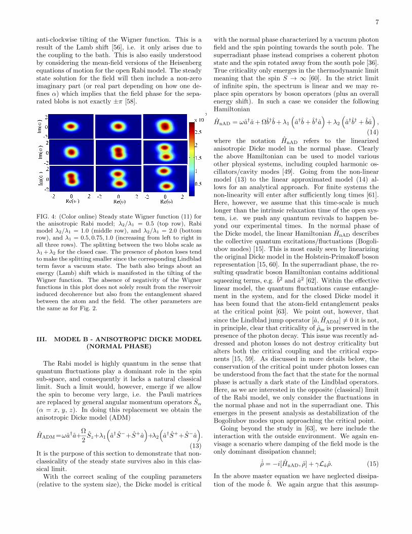
Schrodinger cat [32, 35]. The more resolved the cat statebecomes (the smaller the overlap between the two sepa-rated field states in phase space becomes), the higher theatom-field entanglement obtained. More precisely, these‘dead’ and ‘alive’ field states measure the dipole momentof the atom (corresponding to eigenstates of σx). Thus,when tracing out the atom, the field state will become astatistical mixture between ‘dead’ and ‘alive’. Note thatpure cat state of the form |CAT±〉 ∝ (|α〉 ± | − α〉), forcoherent states | ±α〉 with |α| > 0, have a definite parityand the corresponding photon distributions contain ei-ther only even or odd photon states |n〉. Thus, we ask ifwe can expect a similar statistical cat also for the reduceddensity matrix for the boson field (10)? Figure 2 revealsat least that the photon distribution of the steady stateis super-Poissonian, and combining this with Fig. 3 onemay expect the cat structure to survive photon decay.This should be contrasted with the pioneering experi-ments in the ENS Paris group which measured the decayof the cat into a fully separable atom-field state beforeall photons had leaked the cavity [55]. The phase spacedistribution of the steady state field distribution for theRabi model is indeed split in two as is shown in Fig. 4.The Wigner function for the field mode can be obtainedfrom the following transformation of the density operator

W (α) =2

πTr[D†(α)ρfieldD(α)(−1)a

†a], (11)

where D(α) = exp(αa†−α∗a) is the displacement opera-tor and α = αr + iαm is a complex parameter [56]. Notethat for other expressions for the Wigner function, thereal and imaginary parts of α are related to ‘momentum’p and ‘position’ x. As can be seen from the figure, onincreasing the value of the ratio λ2/λ1 the separation be-tween the two-lobes becomes more pronounced and even-tually the “two-lobes” cease to overlap with each other.A similar two-lobe structure has been found in the tran-sient dynamics of the Wigner function for the dissipativequantum Rabi model with an additional Stark shift termincluded[29]. For the closed system, this behavior readilyfollows from a sort of mean-field approach identical to theBorn-Oppenheimer approximation [32, 57]. In particular,within this approximation and for γ = 0 the maxima ofthe Wigner function are found for

Im(α) =

0, g ≤ gc

±√

g2

ω2 − Ω2

16g2 , g > gc

, (12)

where g = (λ1 + λ2)/2 and gc =√ωΩ/2, and Re(α) ≡ 0.

Note that gc coincide with the critical coupling of theDicke model [36]. Thus, the splitting grows approxi-mately linear with λ1 + λ2. If the signs of the couplingsλ1 and λ2 are different the roles of the real and imag-inary parts of α are interchanged. Now, Fig. 4 showsthat the real parts for the locations of the Wigner func-tion maxima are actually non-zero. This is seen in the

7

anti-clockwise tilting of the Wigner function. This is aresult of the Lamb shift [56], i.e. it only arises due tothe coupling to the bath. This is also easily understoodby considering the mean-field versions of the Heisenbergequations of motion for the open Rabi model. The steadystate solution for the field will then include a non-zeroimaginary part (or real part depending on how one de-fines α) which implies that the field phase for the sepa-rated blobs is not exactly ±π [58].

FIG. 4: (Color online) Steady state Wigner function (11) forthe anisotropic Rabi model; λ2/λ1 = 0.5 (top row), Rabimodel λ2/λ1 = 1.0 (middle row), and λ2/λ1 = 2.0 (bottomrow), and λ1 = 0.5, 0.75, 1.0 (increasing from left to right inall three rows). The splitting between the two blobs scale asλ1 +λ2 for the closed case. The presence of photon loses tendto make the splitting smaller since the corresponding Lindbladterm favor a vacuum state. The bath also brings about anenergy (Lamb) shift which is manifested in the tilting of theWigner function. The absence of negativity of the Wignerfunctions in this plot does not solely result from the reservoirinduced decoherence but also from the entanglement sharedbetween the atom and the field. The other parameters arethe same as for Fig. 2.

III. MODEL B - ANISOTROPIC DICKE MODEL(NORMAL PHASE)

The Rabi model is highly quantum in the sense thatquantum fluctuations play a dominant role in the spinsub-space, and consequently it lacks a natural classicallimit. Such a limit would, however, emerge if we allowthe spin to become very large, i.e. the Pauli matricesare replaced by general angular momentum operators Sα(α = x, y, z). In doing this replacement we obtain theanisotropic Dicke model (ADM)

HADM =ωa†a+Ω

2Sz+λ1

(a†S−+S+a

)+λ2

(a†S++S−a

).

(13)It is the purpose of this section to demonstrate that non-classicality of the steady state survives also in this clas-sical limit.

With the correct scaling of the coupling parameters(relative to the system size), the Dicke model is critical

with the normal phase characterized by a vacuum photonfield and the spin pointing towards the south pole. Thesuperradiant phase instead comprises a coherent photonstate and the spin rotated away from the south pole [36].True criticality only emerges in the thermodynamic limitmeaning that the spin S → ∞ [60]. In the strict limitof infinite spin, the spectrum is linear and we may re-place spin operators by boson operators (plus an overallenergy shift). In such a case we consider the followingHamiltonian

HnAD = ωa†a+ Ωb†b+ λ1

(a†b+ b†a

)+ λ2

(a†b† + ba

),

(14)

where the notation HnAD refers to the linearizedanisotropic Dicke model in the normal phase. Clearlythe above Hamiltonian can be used to model variousother physical systems, including coupled harmonic os-cillators/cavity modes [49]. Going from the non-linearmodel (13) to the linear approximated model (14) al-lows for an analytical approach. For finite systems thenon-linearity will enter after sufficiently long times [61].Here, however, we assume that this time-scale is muchlonger than the intrinsic relaxation time of the open sys-tem, i.e. we push any quantum revivals to happen be-yond our experimental times. In the normal phase ofthe Dicke model, the linear Hamiltonian HnAD describesthe collective quantum excitations/fluctuations (Bogoli-ubov modes) [15]. This is most easily seen by linearizingthe original Dicke model in the Holstein-Primakoff bosonrepresentation [15, 60]. In the superradiant phase, the re-sulting quadratic boson Hamiltonian contains additional

squeezing terms, e.g. b2 and a2 [62]. Within the effectivelinear model, the quantum fluctuations cause entangle-ment in the system, and for the closed Dicke model ithas been found that the atom-field entanglement peaksat the critical point [63]. We point out, however, that

since the Lindblad jump operator [a, HADM] 6= 0 it is not,in principle, clear that criticality of ρss is preserved in thepresence of the photon decay. This issue was recently ad-dressed and photon losses do not destroy criticality butalters both the critical coupling and the critical expo-nents [15, 59]. As discussed in more details below, theconservation of the critical point under photon losses canbe understood from the fact that the state for the normalphase is actually a dark state of the Lindblad operators.Here, as we are interested in the opposite (classical) limitof the Rabi model, we only consider the fluctuations inthe normal phase and not in the superradiant one. Thisemerges in the present analysis as destabilization of theBogoliubov modes upon approaching the critical point.

Going beyond the study in [63], we here include theinteraction with the outside environment. We again en-visage a scenario where damping of the field mode is theonly dominant dissipation channel;

˙ρ = −i[HnAD, ρ] + γLaρ. (15)

In the above master equation we have neglected dissipa-

tion of the mode b. We again argue that this assump-

8

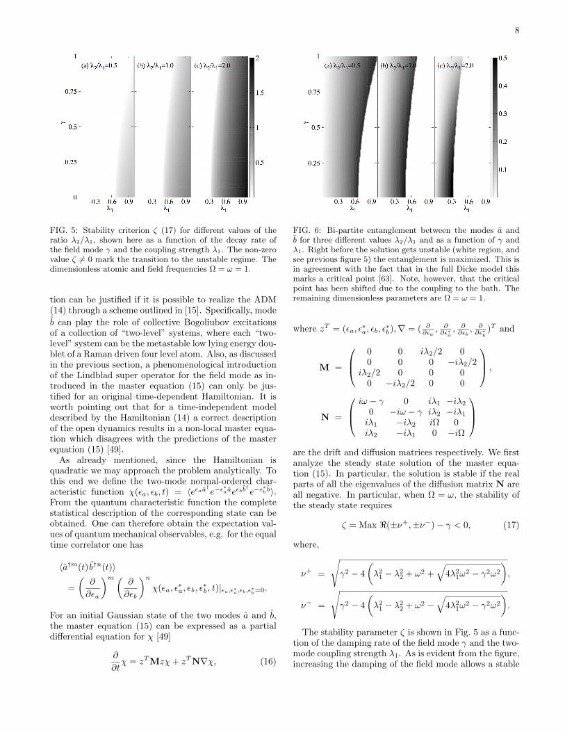
FIG. 5: Stability criterion ζ (17) for different values of theratio λ2/λ1, shown here as a function of the decay rate ofthe field mode γ and the coupling strength λ1. The non-zerovalue ζ 6= 0 mark the transition to the unstable regime. Thedimensionless atomic and field frequencies Ω = ω = 1.

tion can be justified if it is possible to realize the ADM(14) through a scheme outlined in [15]. Specifically, mode

b can play the role of collective Bogoliubov excitationsof a collection of “two-level” systems, where each “two-level” system can be the metastable low lying energy dou-blet of a Raman driven four level atom. Also, as discussedin the previous section, a phenomenological introductionof the Lindblad super operator for the field mode as in-troduced in the master equation (15) can only be jus-tified for an original time-dependent Hamiltonian. It isworth pointing out that for a time-independent modeldescribed by the Hamiltonian (14) a correct descriptionof the open dynamics results in a non-local master equa-tion which disagrees with the predictions of the masterequation (15) [49].

As already mentioned, since the Hamiltonian isquadratic we may approach the problem analytically. Tothis end we define the two-mode normal-ordered char-acteristic function χ(εa, εb, t) = 〈eεaa†e−ε∗aaeεbb†e−ε∗b b〉.From the quantum characteristic function the completestatistical description of the corresponding state can beobtained. One can therefore obtain the expectation val-ues of quantum mechanical observables, e.g. for the equaltime correlator one has

〈a†m(t)b†n(t)〉

=

(∂

∂εa

)m (∂

∂εb

)n

χ(εa , ε∗a , εb , ε

∗b , t)|εa ,ε∗a ,εb ,ε∗b =0.

For an initial Gaussian state of the two modes a and b,the master equation (15) can be expressed as a partialdifferential equation for χ [49]

∂

∂tχ = zTMzχ+ zTN∇χ, (16)

FIG. 6: Bi-partite entanglement between the modes a andb for three different values λ2/λ1 and as a function of γ andλ1. Right before the solution gets unstable (white region, andsee previous figure 5) the entanglement is maximized. This isin agreement with the fact that in the full Dicke model thismarks a critical point [63]. Note, however, that the criticalpoint has been shifted due to the coupling to the bath. Theremaining dimensionless parameters are Ω = ω = 1.

where zT = (εa, ε∗a, εb, ε

∗b),∇ = ( ∂

∂εa, ∂∂ε∗a

, ∂∂εb, ∂∂ε∗b

)T and

M =

0 0 iλ2/2 00 0 0 −iλ2/2

iλ2/2 0 0 00 −iλ2/2 0 0

,

N =

iω − γ 0 iλ1 −iλ2

0 −iω − γ iλ2 −iλ1

iλ1 −iλ2 iΩ 0iλ2 −iλ1 0 −iΩ

are the drift and diffusion matrices respectively. We firstanalyze the steady state solution of the master equa-tion (15). In particular, the solution is stable if the realparts of all the eigenvalues of the diffusion matrix N areall negative. In particular, when Ω = ω, the stability ofthe steady state requires

ζ = Max <(±ν+,±ν−)− γ < 0, (17)

where,

ν+ =

√γ2 − 4

(λ2

1 − λ22 + ω2 +

√4λ2

1ω2 − γ2ω2

),

ν− =

√γ2 − 4

(λ2

1 − λ22 + ω2 −

√4λ2

1ω2 − γ2ω2

).

The stability parameter ζ is shown in Fig. 5 as a func-tion of the damping rate of the field mode γ and the two-mode coupling strength λ1. As is evident from the figure,increasing the damping of the field mode allows a stable

9

steady state to be achieved for an extended region of pa-rameter space spanned by λ1. This behavior can be un-derstood physically by considering the different terms ofthe master equation (15). First we may note that the in-stability of the mode coincides with the Dicke phase tran-sition. Indeed, the model Hamiltonian (14) describes thecollective excitations in the normal phase and not in thesuperradiant phase, and hence, these excitation modescannot be analytically continued into the superradiantphase. Thus, we conclude that increasing the photon lossgives a more extended normal phase. This is expectedsince the Lindblad term of Eq. (15) favors the vacuumstate of the field, which is also favored by the bare fieldenergy ωa†a. On the other hand, the atom-field couplingterm is not minimized by such a field state. Without pho-ton decay, the transition occurs at (λ1 + λ2) =

√ωΩ (see

Eq. (15)), but now losses support the normal phase andthereby shift the critical value. Following Refs. [15, 64]

one explicitly finds λc =√

Ω (ω2 + γ2) /ω/2 which is ob-tained at the mean-field level, i.e. in the thermodynamiclimit. In the Dicke limit (λ1 = λ2 = λ) it is easy to obtainthe phase boundary ω2 + γ2 = 4λ2, which retrieves theresult for the critical coupling of the open Dicke modelon resonance [15, 64].

The steady state of light-matter coupled quantum sys-tem modeled under the master equation (6) was shownto be an inseparable state of the cavity field and thetwo-level system. Somewhat surprisingly, this observa-tion can also be extended to the steady state of thenormal phase of the Dicke model (15). In particu-lar, one could argue that in the thermodynamic limitas studied here any entanglement should vanish sincefor the Dicke model quantum fluctuations are negligi-ble [65]. That this is not the case derives from the pres-ence of the critical point. To demonstrate sustainablequantum correlations we next evaluate the steady statebi-partite entanglement between the two modes a and

b and characterize it in terms of the logarithmic neg-ativity which for two-mode Gaussian states serves asa necessary and sufficient criterion for the inseparabil-ity [66]. A two-mode Gaussian state can be fully quanti-fied in terms of its covariance matrix V which is a 4× 4symmetric matrix with Vij = (〈RiRj + RjRi〉)/2 andRT = (qa, pa, qb, pb). Here qa,b and pa,b are the posi-

tion and momentum quadratures of the mode a(b). Fora two-mode Gaussian continuous-variable state with co-variance matrix V, the logarithmic negativity is obtainedas N = Max[0,−log(2ν−)] [66], where ν− is the smallestof the symplectic eigenvalues of the covariance matrix,

given by ν− =√σ/2−

√(σ2 − 4DetV)/2. Here

σ = DetA1 + DetB1 − 2DetC1

V =

(A1 C1

CT1 B1

),

where A1 (B1) accounts for the local variances of modea (b) and C1 for the inter-mode correlations. Using thenumerical solutions of the partial differential equations

(16) we compute the logarithmic negativity. The steadystate two-mode entanglement is shown in Fig. 6 whereit is given as a function of the damping rate γ and thetwo-mode coupling strength λ1. As is evident, the maxi-mum attainable bi-partite entanglement between the twomodes monotonically increases on increasing the valueof the ratio λ2/λ1. The highest entanglement is ob-tained at the critical point, which is also known fromthe closed Dicke model [63]. This is, in fact, a generalproperty for quantum phase transitions; at the criticalpoint where characteristic length scales diverge, the en-tanglement also diverges [67]. However, already for theclosed Dicke model the phase transition is not a ‘typical’quantum phase transition since there is no length scalein the problem and, as we mentioned above, quantumfluctuations vanish in the thermodynamic limit. Becauseof this, the transition has been called ‘classical’ [65]. Assuch, the results of Fig. 6 suggest that, qualitatively, thesame behavior of the entanglement is found for a dynam-ical phase transition of an open driven system.

IV. QUANTUM CONTROL IN HYBRIDARCHITECTURES

FIG. 7: Schematic plot of the feedback loop between the twocavities. We envision a scenario of two coupled cavities; asource cavity and a driven cavity. The driven cavity is as-sumed to be slaved to the source cavity. The source cavitydrives the state of the slave cavity by means of a unidirec-tional coupling (shown by a solid line). The driven cavity inturn also influences the state of the source cavity by meansof a reversible interaction (shown by a dotted line). The si-multaneous presence of reversible and irreversible couplingsbetween the cavity modes results in an all-optical feedbackloop.

In the previous two sections we have studied the opendynamics of the anisotropic Rabi and Dicke models andhave explicitly explored the properties of the NESSs ofthese models. However, so far we have eluded ourselvesfrom effectively engineering the open dynamics of thesehybrid models. Even though it was found that entangle-ment persists in both models despite losses, in the presentsection we wish to explore the possibilities to enhance theamount of entanglement by actively introducing feedbackinto the model.

An unusual ingredient which enriches the dynamics ofquantum systems is their inherent ‘openness’ which may

10

FIG. 8: Illustration of the general all-optical feedback of Fig. 7specifically used for establishing quantum control in the Dickemodel of Section III. The internal dynamics of the source cav-ity is modeled by (14) while the driven cavity is initially pre-pared in its vacuum state. Mode a of the source cavity andthe mode c of the driven cavity are interacting under a re-versible interaction of the form (18). Mode a of the sourcecavity also couples irreversibly to mode c of the driven cav-ity. Such a feed-forward coupling can be engineered throughfeeding the mode a from one end of the source cavity andreflecting it onto the driven cavity through a series of mirrors(filled) and beam-splitters (unfilled). Optical circulators orFaraday isolators can be used to prevent interference from re-flections in the opposite directions. Reversible and irreversibleinteractions jointly constitute an all-optical feedback. If thisfeedback loop has negligible time delay a Markovian masterequation to describe the open dynamics of the source cavitycan be derived (21) as detailed in Section IV A.

result in exotic NESS properties [9, 11, 48, 68, 69]. Thiswas in particular the theme of the previous two sections.However, engineering a controlled degree of dissipationis also an important tool in realizing tasks of quantuminformation processing. In this spirit we will now use anall-optical feedback scheme for quantum state protectionand establishing quantum control in the normal phaseof the Dicke model. The scheme we choose is based oncoherent feedback, i.e. no measurement is performed inthe feedback loop [16]. A symbolic plot of a coherent(all-optical) feedback scheme is illustrated in Fig. 7; itcomprises of two units, which have been labeled sourceand driven cavities, with reversible and irreversible cou-plings between them. The simplest all optical feedbackloop will use the output from a source cavity and feedfor-ward into a driven cavity which is coupled to the sourcecavity in some way. It is worth mentioning that unidirec-tional and bidirectional couplings between the source andthe driven cavities jointly constitute an all optical feed-back scheme. A coherent feedback loop, however, canalso introduce a finite time-delay τ . Firstly, assumingthat the time-delay τ introduced by the feedback loop isnegligible, we study the open dynamics of the source cav-ity [18–20]. Subsequently, making use of a time-delayedfeedback control method, [21–23] we incorporate a time-delay τ introduced by the feedback loop.

A. All optical feedback loop with negligibletime-delay τ

We now apply the general scheme of all-optical feed-back illustrated in Fig. 7 for a specific task of quantumstate protection in the anisotropic Dicke model of Sec.III. A schematic of our proposal to implement all-opticalfeedback is shown in Fig. 8. The internal (unitary) dy-namics of the source cavity is described by the Hamilto-nian (14), i.e. Hsource = HnAD and the driven cavity isreversibly coupled to the field mode of the source cavityby the following Hamiltonian [18, 19]

Hint = iµ

√γγd

2(a†c− c†a), (18)

where µ is a dimensionless coupling parameter, c† and care the creation and annihilation operators for the fieldmode of the driven cavity which has damping rate γd.The driven cavity is assumed to be prepared in its vac-uum state with its respective internal dynamics modeledas Hdriven = Ωdc

†c. A reversible interaction of the form(18) can arise through mode overlap between the modesa and c [70].

Under the Born-Markov approximation a joint state ofthe source and driven cavities, represented here as W ,evolves under the following master equation [16, 18, 19]

˙W = −i

[HnAD +Hdriven + Hint, W

]+√γγd([aW , c†] + [c, W a†])

+γ

2LaW +

γd

2LcW . (19)

It should be remarked that W represents a tri-partite

state of modes a, b, and c. On the grounds of argumentspresented previously, we have again neglected damping

of the mode b of the source cavity. The two terms ap-pearing in the second line account for the unidirectionalcoupling between the source and driven cavities and thelast two terms are the individual Lindblad operators de-scribing photon losses for the source and driven cavitymodes respectively. As illustrated in Fig. 8, such a uni-directional coupling between the source and driven cavi-ties can be established using an optical circulator [18]: anon-reciprocal optical device such as Faraday rotator canbe used to establish irreversible coupling between the op-tical modes a and c of the source and the driven cavities.As pointed out in Refs. [18, 19], for the feedback loop tobe effective the driven cavity should respond much fasterthan the source cavity. We thus work in a regime whereγd 1 meaning that the state of the driven cavity isslaved to the state of the source cavity. Since γd is thelarge parameter (i.e. determining the fast time scale) andthe driven cavity is assumed to couple to a zero temper-ature reservoir, the population of the driven cavity modecan be truncated to only the lowest photon states. Wetherefore approximate the joint state of the two coupled

11

cavities as

W = ρ00|0〉〈0|+ ρ10|1〉〈0|+ ρ†10|0〉〈1|+ρ11|1〉〈1|+ ρ20|2〉〈0|+ ρ†20|0〉〈2|, (20)

where ρij is the conditional state of the source cavity

(a joint state of modes a and b) when the driven cavityis projected on the state space |i〉〈j|. Using the aboveansatz and adiabatically eliminating the driven cavity itis possible to derive an effective master equation for thesource cavity alone [18, 19]. Following the derivation pro-vided in Appendix A one arrives at the resulting masterequation

˙ρ = ˙ρ00 + ˙ρ11 = −i[HnAD, ρ

]+γeff

2Laρ, (21)

where γeff = γ (1 + µ(2 + µ)) is the new effective damp-ing rate of the field mode. On choosing the dimensionlessparameter µ = −1, it is remarkable to observe that anall optical feedback loop is capable of completely block-ing the loss of the source cavity. However, losses inthe feedback loop would deteriorate the effectiveness ofsuch feedback. If the feedback loop has an efficiencyη (≤ 1), then it is possible to show that the effec-tive damping rate of the source cavity gets modified asγeff = γ (1 + ηµ(2 + µ)) [19]. We therefore conclude that,under the assumptions that the time-delay introduced bya feedback loop is negligible and the state of the drivencavity is effectively slaved to the source cavity, it is pos-sible to establish arbitrary control over the damping rateof the source cavity. This can be an important step forquantum state protection in hybrid quantum systems.

As an example application of an all optical feedbackscheme for quantum state protection, we assume that thetwo coupled modes interacting under the Hamiltonian(14) are initially prepared in a NOON state [71]. NOONstates are Bell-like entangled states with applications inquantum metrology and quantum lithography and theymay also be utilized for achieving phase supersensitivity

[72]. We assume that the modes a and b are initialized

in a state |ΨN− 〉 = (|N〉a|0〉b− |0〉aN〉b)/

√2. We examine

the autocorrelation function, i.e. the overlap betweenρ(0) and the time evolving joint state of the two modesρ(t), which for mixed states is given by the Uhlmannfidelity [73, 74]

Φ = Tr

√√ρ(0)ρ(t)

√ρ(0). (22)

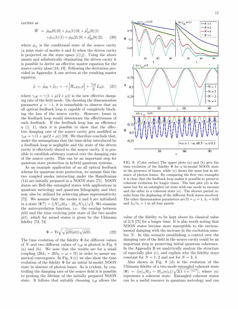
The time evolution of the fidelity Φ for different valuesof N and two different values of γeff is plotted in Fig. 9(a) and (b). We note that the results are for a smallcoupling (20λ1 = 20λ2 = ω = Ω) in order to assure nu-merical convergence. In Fig. 9 (c) we also show the timeevolution of the fidelity Φ for an initial bi-model NOONstate in absence of photon losses. As is evident, by con-trolling the damping rate of the source field it is possibleto prolong the lifetime of the initially prepared NOONstate. It follows that suitably choosing γeff allows the

FIG. 9: (Color online) The upper plots (a) and (b) give thetime evolution of the fidelity Φ for a bi-modal NOON statein the presence of losses, while (c) shows the same but in ab-sence of photon losses. By comparing the first two examplesit is clear that the feedback loop makes it possible to preservecoherent evolution for longer times. The last plot (d) is thesame but for an entangled cat state with one mode in vacuumand the other in a coherent state |α〉. The shorter period re-sults from the dephasing of the different Fock states involved.The other dimensionless parameters are Ω = ω = 1, λ1 = 0.05and λ2/λ1 = 1 in all four panels.

value of the fidelity to be kept above its classical valueof 2/3 [75] for a longer time. It is also worth noting thatNOON states become more susceptible to the environ-mental damping with the increase in the excitation num-ber N . In this scenario establishing a control over thedamping rate of the field in the source cavity could be animportant step in preserving initial quantum coherence.In the Appendix B we analytically analyze the structureof especially plot (c), and explain why the fidelity staysconstant for N = 1, 2 and not for N = 3, 4.

Also shown in Fig. 9 (d) is the evolution of theUhlmann fidelity of a two-mode entangled coherent state

|Ψ〉 = (|α〉a|0〉b + |0〉a|α〉b)/√

2(1 + e−|α|2), where |α〉represents a coherent state. Entangled coherent statescan be a useful resource in quantum metrology and can

12

exhibit noticeable improved sensitivity for phase estima-tion when compared to that for NOON states. Entangledcoherent states can also outperform the phase enhance-ment achieved by NOON states both in the lossless, weak,moderate and high loss regimes [76]. As demonstrated inFig. 9 (d), when compared to a NOON state a two-modeentangled coherent state is found to be more resilient tophoton losses. Nevertheless, the quantum fidelity of en-tangled coherent states also seems to decay significantlywith the increase in the mean number of photons |α|2.

B. All optical feedback loop with finite time-delayτ

As mentioned before, in deriving the master equation(21) it has been assumed that the time-delay τ intro-duced by the feedback loop is negligible [18]. In thissection we explore a complementary regime when thefeedback loop introduces a non-negligible time-delay τ .In particular, we use the time-delayed feedback controlmethod of Ref. [21–23] and apply it to our Hamiltonian(14). We refer the reader to [23] for a specific proposalimplementing a finite time-delay in an optical feedbackloop and applying it to the Dicke model (14). In thiswork we go beyond the analysis presented in [23] and willinclude quantum fluctuations to check the steady statestability of the time-delayed feedback control scheme and

to compute steady state correlations between modes a, b.Considering a specific all-optical time-delayed feedbackcontrol strategy discussed in detail in [23] and apply-ing it to our Hamiltonian (14) we arrive at the followingHeisenberg-Langevin equations of motion (14)

d

dtV(t)T = AV(t)T −BV(t)T

−√

2Γ Vin(t)T + BV(t− τ)T , (23)

where

V(t) = (a(t), a†(t), b(t), b†(t)),

V(t− τ) = (a(t− τ), a†(t− τ), b(t− τ), b†(t− τ)),

Vin(t) = (ain(t), a†in(t), 0, 0),

A =

−iω − γ 0 −iλ1 −iλ2

0 iω − γ iλ2 iλ1

−iλ1 −iλ2 −iΩ 0iλ2 iλ1 0 iΩ

,

B =

γ/2 0 0 00 γ/2 0 00 0 0 00 0 0 0

.

(24)Here, Vin(t) contains the input noise terms [77]. It shouldbe pointed out that in writing the above Heisenberg-

Langevin equations we have assumed that the time-delayed feedback loop has unit efficiency [23]. To con-nect with the approach of the previous sections, we haveagain assumed that the damping of the mode a is the onlydominant channel of dissipation. Also, the time-delayedcontrol feedback strategy (23) is implemented through acontrol force which is generated from the difference be-tween the instantaneous cavity field a(t) and the field atsome point in the past a(t− τ) [23].

As a first step to check the influence of the time-delayedfeedback control on our hybrid quantum system we checkthe stability of the above Heisenberg-Langevin equationssemi-classically, i.e. we assume the noise 〈Vin(t)〉=0. Us-ing an ansatz V (t) ∼ eΛt we get the following secularequation [21, 22]

det(A−B + Be−Λτ − Λ1). (25)

For a non-zero value of τ , this transcendental equationhas an infinite set of complex solutions for eigenvalues Λ.The steady state is stable only if the real parts of all thesolutions Λ are negative [21, 22]. We numerically solvethe above secular equation (25) for all possible roots Λ.In doing so we choose λ1 and γ such that in the absenceof a time-delayed feedback loop the steady state is stablefor all values of the ratio 0 ≤ λ2/λ1 ≤ 2, see Fig. 5. InFig. 10 we plot the maximum of the real part of all possi-ble solutions Λ. We find that at a semiclassical level, andfor the set of parameters considered in Fig. 10, our time-delayed feedback control strategy does not qualitativelyalter the stability of the steady state.

FIG. 10: (Color online) Maximum of the real part of all pos-sible solutions of the secular equation (25) for three differentvalues of the ratio λ2/λ1 and shown here as a function ofthe time-delay τ . The dimensionless parameters have beentaken Ω = ω = 1, λ1 = 0.1 and γ = 0.1. For these set ofparameters the steady state is stable for all values of the ra-tio 0 ≤ λ2/λ1 ≤ 2 in the absence of a time-delayed feedbackloop, see Fig. 5.

To show that our time-delayed feedback control strat-egy is indeed capable of influencing the steady state be-haviour of our hybrid quantum system, we now embarkon a full quantum treatment to explore the steady state

correlations between the modes a and b with their dy-namics governed by Eq. (23). We solve the equations inthe Fourier space and reconstruct the steady state two-

13

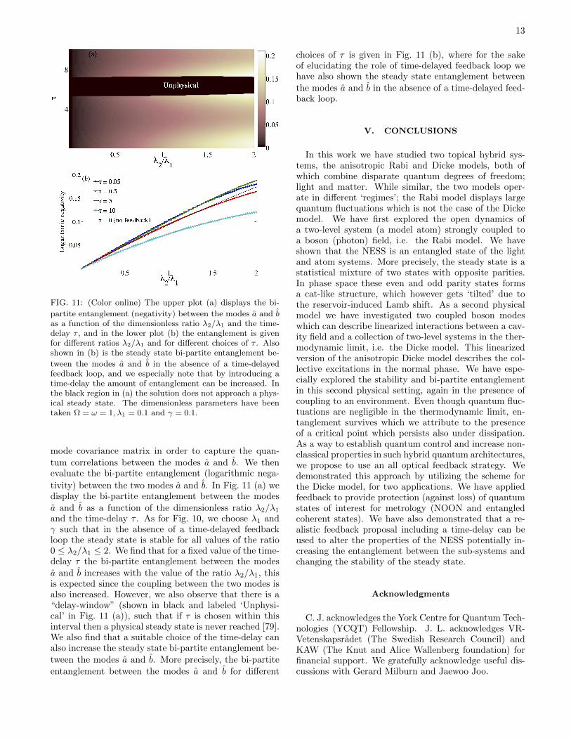
FIG. 11: (Color online) The upper plot (a) displays the bi-

partite entanglement (negativity) between the modes a and bas a function of the dimensionless ratio λ2/λ1 and the time-delay τ , and in the lower plot (b) the entanglement is givenfor different ratios λ2/λ1 and for different choices of τ . Alsoshown in (b) is the steady state bi-partite entanglement be-

tween the modes a and b in the absence of a time-delayedfeedback loop, and we especially note that by introducing atime-delay the amount of entanglement can be increased. Inthe black region in (a) the solution does not approach a phys-ical steady state. The dimensionless parameters have beentaken Ω = ω = 1, λ1 = 0.1 and γ = 0.1.

mode covariance matrix in order to capture the quan-

tum correlations between the modes a and b. We thenevaluate the bi-partite entanglement (logarithmic nega-

tivity) between the two modes a and b. In Fig. 11 (a) wedisplay the bi-partite entanglement between the modes

a and b as a function of the dimensionless ratio λ2/λ1

and the time-delay τ . As for Fig. 10, we choose λ1 andγ such that in the absence of a time-delayed feedbackloop the steady state is stable for all values of the ratio0 ≤ λ2/λ1 ≤ 2. We find that for a fixed value of the time-delay τ the bi-partite entanglement between the modes

a and b increases with the value of the ratio λ2/λ1, thisis expected since the coupling between the two modes isalso increased. However, we also observe that there is a“delay-window” (shown in black and labeled ‘Unphysi-cal’ in Fig. 11 (a)), such that if τ is chosen within thisinterval then a physical steady state is never reached [79].We also find that a suitable choice of the time-delay canalso increase the steady state bi-partite entanglement be-

tween the modes a and b. More precisely, the bi-partite

entanglement between the modes a and b for different

choices of τ is given in Fig. 11 (b), where for the sakeof elucidating the role of time-delayed feedback loop wehave also shown the steady state entanglement between

the modes a and b in the absence of a time-delayed feed-back loop.

V. CONCLUSIONS

In this work we have studied two topical hybrid sys-tems, the anisotropic Rabi and Dicke models, both ofwhich combine disparate quantum degrees of freedom;light and matter. While similar, the two models oper-ate in different ‘regimes’; the Rabi model displays largequantum fluctuations which is not the case of the Dickemodel. We have first explored the open dynamics ofa two-level system (a model atom) strongly coupled toa boson (photon) field, i.e. the Rabi model. We haveshown that the NESS is an entangled state of the lightand atom systems. More precisely, the steady state is astatistical mixture of two states with opposite parities.In phase space these even and odd parity states formsa cat-like structure, which however gets ‘tilted’ due tothe reservoir-induced Lamb shift. As a second physicalmodel we have investigated two coupled boson modeswhich can describe linearized interactions between a cav-ity field and a collection of two-level systems in the ther-modynamic limit, i.e. the Dicke model. This linearizedversion of the anisotropic Dicke model describes the col-lective excitations in the normal phase. We have espe-cially explored the stability and bi-partite entanglementin this second physical setting, again in the presence ofcoupling to an environment. Even though quantum fluc-tuations are negligible in the thermodynamic limit, en-tanglement survives which we attribute to the presenceof a critical point which persists also under dissipation.As a way to establish quantum control and increase non-classical properties in such hybrid quantum architectures,we propose to use an all optical feedback strategy. Wedemonstrated this approach by utilizing the scheme forthe Dicke model, for two applications. We have appliedfeedback to provide protection (against loss) of quantumstates of interest for metrology (NOON and entangledcoherent states). We have also demonstrated that a re-alistic feedback proposal including a time-delay can beused to alter the properties of the NESS potentially in-creasing the entanglement between the sub-systems andchanging the stability of the steady state.

Acknowledgments

C. J. acknowledges the York Centre for Quantum Tech-nologies (YCQT) Fellowship. J. L. acknowledges VR-Vetenskapsradet (The Swedish Research Council) andKAW (The Knut and Alice Wallenberg foundation) forfinancial support. We gratefully acknowledge useful dis-cussions with Gerard Milburn and Jaewoo Joo.

14

Appendix A: Markovian master equation withoptical feedback

In this appendix we provide the details of the deriva-tion of the master equation (21). For the feedback loop tobe effective, the driven cavity should respond much fasterthan the source cavity. We thus work in a regime whereγd 1 and the state of the driven cavity follows adiabat-ically the evolution of the source cavity. The large decayrate and the coupling to a zero temperature reservoirimplies that driven cavity may only be weakly excited,which justifies the ansatz state (20). With such a jointstate of two coupled cavities one obtains the followingequations of motion for the source cavity

˙ρ00 = −i[HnAD, ρ00

]+γ

2Laρ00 + γdρ11

+√γγd(aρ†10 + ρ10a

†) + µ

√γγd

2(a†ρ10 + ρ†10a)

˙ρ10 = −i[HnAD, ρ10

]+γ

2Laρ10 −

γd

2ρ10

+√γγd(aρ11 − aρ00 +

√2ρ20a

†)

+µ

√γγd

2(√

2a†ρ20 − aρ00 + ρ11a)

˙ρ11 = −i[HnAD, ρ11

]+γ

2Laρ11 − (iΩd + γd)ρ11

−√γγd(aρ†10 + ρ10a†)− µ

√γγd

2(aρ†10 + ρ10a

†)

˙ρ20 = −i[HnAD, ρ20

]+γ

2Laρ20 − 2γdρ20

−√

2γγdaρ10 − µ√γγd√2aρ10.

The state of the source cavity is of interest to us andit can be extracted as ρ = TrcW = ρ00 + ρ11. From theabove equations, the off-diagonal elements ρ10 and ρ20

can be adiabatically eliminated by slaving them to thediagonal elements ρ00 and ρ11. Setting ˙ρ20=0 we obtainto leading order in 1/

√(γd/γ)

ρ20 = − 1√2(γd/γ)

(µ

2+ 1) a ρ10. (A1)

Inserting the above expression in the steady state equa-tion of ρ10 we obtain

ρ10 =2√

(γd/γ)(µ

2ρ11a−

µ

2aρ00 + aρ11 − aρ00). (A2)

Using the above steady state solution for the off-diagonalelement yields the following master equation for the den-sity matrix of the source cavity alone

˙ρ = ˙ρ00 + ˙ρ11 = −i[HnAD, ρ] +γ

2Laρ− iΩdρ11

+µγ[La(ρ00 − ρ11) +µ

2Laρ00 +

µ

2La† ρ11].(A3)

When γd 1, ρ11 ∼ O(0) and ρ ≈ ρ00 we arrive atthe following master equation approximating the source

dynamics

˙ρ = ˙ρ00 + ˙ρ11 = −i[HnAD, ρ

]+γeff

2Laρ, (A4)

where γeff = γ(1+µ(2+µ)) is the effective damping rateof the field mode in the source cavity.

Appendix B: Uhlmann fidelity in the RWA regime

A conspicuous feature of Fig. 9 (especially in (c)) is thealmost constant evolution of the fidelity for the stateswith N = 1, 2, and the oscillatory structure for theN = 3, 4 states. This implies that |Ψ1,2

− 〉 are station-

ary states while |Ψ3,4− 〉 seems to be formed from two sta-

tionary states. In this appendix we will explain how thiscomes about given the initial states and the Hamiltonian(14). As pointed out in the main text, for the figure asmall coupling has been used (20 times smaller than thebare frequencies) which means that imposing the RWAis justified, i.e. we let λ2 = 0 from now on. We havenumerically verified that the RWA is applicable for thecorresponding parameters.

Now, when λ2 = 0 the Hamiltonian can be readily di-agonalized by defining two new bosonic operators; ‘even’

z+ = (a + b)/√

2 and ‘odd’ z− = (a − b)/√

2. Theseobey the regular boson commutation relations and mu-tually commute. In particular the ‘odd’ Fock states

|n−〉 = z†n−− |0〉/

√n−! have shown to be important for

adiabatic passage in multimode cavities [78]. Expressedwith the new rotated operators, the Hamiltonian is diag-onal

Hz = (ω + λ1)z†+z+ + (ω − λ1)z†−z−. (B1)

It follows that the eigenstates are |n+〉|n−〉 =

z†n+

+ z†n−− |0〉a|0〉b/

√n+!n−!, with corresponding eigenen-

ergies εn+n− = ω (n+ + n−) + λ1 (n+ − n−).For an N particle NOON state we have

|ΨN− 〉 =

1√2N !

(a†N − b†N

)|0〉a|0〉b. (B2)

Thus, we notice that |Ψ1−〉 = z†−|0〉a|0〉b is indeed a sta-

tionary state with its time evolution given by

|Ψ1−(t)〉 = e−i(ω−λ1)t|Ψ1

−〉. (B3)

The time evolved state (B3) is of course strictly only cor-rect within the RWA, and the exact time evolved stateshould be given by evolution under the full Hamiltonian;

|Ψ1exact(t)〉 = e−iHnADt|Ψ1

−〉. Numerically we find the er-ror arriving from neglecting the counter rotating termsδ1 = |Φexact −ΦRWA| < 0.003 for all t. Similarly, we find

that the two particle NOON state |Ψ2−〉 = z†+z

†−|0〉a|0〉b

is also a stationary state with the time evolution

|Ψ2−(t)〉 = e−i2ωt|Ψ2

−〉. (B4)

15

In this case the numerically estimated error δ2 = |Φexact−Φapprox| < 0.004 for all t. Interestingly, the alternative

NOON state |Ψ2+〉 = (|2〉a|0〉b + |0〉|a2〉b)/

√2 is not a

stationary state.Turning now to the N = 3 case. It is easy to show

that there is no N = 3 NOON state (most general form|3〉a|0〉b + eiφ|0〉a|3〉b) that can be a stationary state. Forthe present state the time evolved state takes the form

|Ψ3−(t)〉 =

e−i3ωt

2√

3!(3z†2+ z

†−e−iλ1t + z†3− e

i3λ1t)|0〉a|0〉b.

(B5)It is a straightforward exercise to show that |Ψ3

−(t)〉evolves as a time dependent mixture of the orthogonalstates |Ψ3

−〉 and |Ψ3orth〉 = (|2〉a|1〉b − |1〉a|2〉b)/

√2. But,

never in the course of time evolution the coefficient of|Ψ3−〉 vanishes completely. This is the reason why the

fidelity Φ for N = 3 in Fig. 9 (c) never drops close tozero.

The situation is however somewhat different for|Ψ4−(t)〉 whose time evolution is

|Ψ4−(t)〉 =

e−i4ωt√

2√4!

(z†3+ z†−e−i2λ1t + z†+z

†3− e

i2λ1t)|0〉a|0〉b.

(B6)Even though, like in the N = 3 situation, one cannotfind a general NOON state being a stationary state (infact it is only possible for N = 1, 2), the above timeevolved state evolves into a state completely orthogonalto |Ψ4

−〉. For instance, when 2λ1t = (2m+ 1)π/2 one ob-

tains |Ψ4−(t)〉 ∼ |Ψ4

orth〉 = (|3〉a|1〉b − |1〉a|3〉b)/√

2. Thisis where the fidelity Φ for |Ψ4

−〉 drops close to zero asshown in Fig. 9 (c).

[1] G. Kurizki, P. Bertet, Y. Kubo, K. Mølmer, D. Pet-rosyan, P. Rabl, and J. Schmiedmayer, Proc. Natl. Acad.Sci. U.S.A. 112, 3866(2015).

[2] A. Zeilinger, Rev. Mod. Phys. 71, 288 (1999); A. Blais,J. Gambetta, A Wallraff, D. I. Schuster, S. M. Girvin,M. H. Devoret, and R. J. Schoelkopf, Phys Rev. A 75,032329 (2007).

[3] J. M. Raimond, M. Brune, and S. Haroche, Rev. Mod.Phys. 73, 565 (2001).

[4] D. Loss and D. P. DiVincenzo, Phys. Rev. A 57, 120(1998).

[5] U. Weiss,Quantum Dissipative Systems (World Scientific,Singapore, 1993).

[6] H.-P. Breuer and F. Petruccione, The Theory of OpenQuantum Systems (Oxford University Press, Oxford,2002).

[7] W. H. Zurek, Rev. Mod. Phys. 75, 715 (2003).[8] ZL Xiang, S. Ashhab, J. Q. You, and F. Nori, Rev. Mod.

Phys. 85, 623 (2013).[9] F. Verstraete, M. M. Wolf, and J. I. Cirac, Nature Phys.

5, 633 (2009); J. T. Barreiro, M. Muller, P. Schindler, D.Nigg, T. Monz, M. Chwalla, M. Hennrich, C. F. Roos, P.Zoller, and R. Blatt, Nature 470 486 (2011); Y. Lin, J. P.Gaebler, F. Reiter, T. R. Tan, R. Bowler, A. S. Sørensen,D. Leibfried, and D. J. Wineland, Nature 504 415 (2013);D. V. Vasilyev, C. A. Muschik, and K. Hammerer, Phys.Rev. A 87, 053820 (2013).

[10] S. Diehl, A. Micheli, A. Kantian, B. Kraus, H. P. Buchler,and P. Zoller, Nature Phys. 4, 878 (2008); M Muller, SDiehl, G Pupillo, and P Zoller, Adv. Atom. Mol. Opt.Phys 61, 1 (2012).

[11] C. Joshi, F. Nissen, and J. Keeling, Phys. Rev. A 88,063835 (2013).

[12] I. I. Rabi, Phys. Rev. 49, 324 (1936); 51, 652 (1937).[13] E. T. Jaynes and F. W. Cummings, Proc. IEEE 51, 89

(1963).[14] R . H. Dicke, Phys. Rev. 93, 99 (1954); B. M. Garraway,

Phil. Trans. R. Soc. A 369, 1137 (2011).[15] F. Dimer, B. Estienne, A. S. Parkins and H. J.

Carmichael, Phys. Rev. A 75, 013804 (2007).[16] H. M. Wiseman, and G. J. Milburn, Quantum Measure-

ment and Control (Cambridge Univ. Press, 2010).[17] P. Rabl, D. DeMille, J. M. Doyle, M. D. Lukin, R. J.

Schoelkopf, and P. Zoller, Phys. Rev. Lett. 97, 033003(2006).

[18] H. M. Wiseman and G. J. Milburn, Phys. Rev. A 49,4110 (1994).

[19] P. Tombesi, V. Giovannetti, and D. Vitali, in “Directionsin Quantum Optic”, edited by H. J. Carmichael, R. J.Glauber, and M. O. Scully, Lecture Notes in Physics 561,204 (2001).

[20] C. Joshi, U. Akram, G. J. Milburn, New J. Phys. 16023009 (2014).

[21] K. Pyragas, Phys. Lett. A 170 421(1992); J. E. S. Soco-lar, D.W. Sukow, and D.J. Gauthier, Phys. Rev. E 503245(1994); D. J. Gauthier, D.W. Sukow, H.M. Concan-non, and J.E.S. Socolar, Phys. Rev. E 50 2343(1994); P.Hovel and E. Scholl, Phys. Rev. E 72, 046203 (2005).

[22] N. Yamamoto, Phys. Rev. X 4, 041029 (2014); Carmele,J. Kabuss, F. Schulze, S. Reitzenstein, and A. Knorr,Phys. Rev. Lett. 110, 013601 (2013); Y.-L. L. Fang andH. U. Baranger, Phys. Rev. A 91,053845 (2015); Was-silij Kopylov, Clive Emary, Eckehard Scholl and TobiasBrandes, New J. Phys. 17, 013040 (2015).

[23] A. L. Grimsmo, A. S. Parkins and B.-S. Skagerstam, NewJ. Phys. 16 065004 (2014).

[24] D. Braak, Phys. Rev. Lett. 107, 100401 (2011).[25] A. Moroz, Annals Phys. 338, 319 (2013).[26] For a brief review see [24, 27–29] and references therein.[27] E. Solano, Physics 4 68 (2011).[28] D. Ballester, G. Romero, J. J. Garcıa-Ripoll, F.

Deppe,and E. Solano, Phys. Rev. X 2, 021007 (2012).[29] A. L. Grimsmo, and S. Parkins, Phys. Rev. A 87 033814

(2013).[30] B. W. Shore and P. L. Knight, J. Mod. Opt. 40, 1195

(1993).[31] D. Leibfried, R. Blatt, C. Monroe, and D. Wineland, Rev.

Mod. Phys. 75, 281 (2003).[32] J. Larson, Phys. Scr. 76, 146 (2007).[33] T. Niemczyk, F. Deppe, H. Huebl, E. P. Menzel, F.

Hocke, M. J. Schwarz, J. J. Garcia-Ripoll, D. Zueco, T.Hmmer, E. Solano, A. Marx , and R. Gross, Nature, 6

16

772 (2010).[34] J. Q. You, and F. Nori, Nature 474, 589 (2011).[35] E. K. Irish, J. Gea-Banacloche, I. Martin, and K. C.

Schwab, Phys. Rev. B 72, 195410 (2005).[36] K. Hepp and E. H. Lieb, Annals Phys. 76, 360 (1973); C.

Emary and T. Brandes, Phys. Rev. E 67, 066203 (2003).[37] J. Casanova, G. Romero, I. Lizuain, J. J. Garca-Ripoll,

and E. Solano, Phys. Rev. Lett. 105, 263603 (2010).[38] See Ref. [39]. We do, however, also refer the reader to

[40] for a recent proposal on simulating the ultra-strongand deep strong coupling regimes of quantum Rabi modelwith trapped ions.

[39] A. Vukics, T. Grießer, and P. Domokos, Phys. Rev. Lett.112, 073601 (2014).

[40] J. S. Pedernales, I. Lizuain, S. Felicetti, G. Romero,L. Lamata, and E. Solano, Scientific Reports 5 15472(2015).

[41] K. Rzazewski, K. Wodkiewicz, and W. Zakowicz, Phys.Rev. Lett. 35, 432 (1975). See however A. Vukics, T.Grießer, and P. Domokos, Phys. Rev. Lett. 112, 073601(2014) where it is shown that the transition might occur ifa self-consistent quantization of the system is considered.

[42] Q.-T. Xie, S. Cui, J.-P. Cao, L. Amico, and H. Fan, Phys.Rev. X 4 021046 (2014).

[43] Y. Y. Xiang, J. Ye, and W. M. Liu, Scientific Reports 3,3476 (2013).

[44] P. Lougovski, E. Solano, and H. Walther, Phys. Rev. A71, 013811 (2005).

[45] J. Mumford, J. Larson, and D. H. J. O’Dell, Phys. Rev.A 89, 023620 (2014).

[46] M.-J. Hwang, R. Puebla, and M. B. Plenio, Phys. Rev.Lett. 115, 180404 (2015).

[47] M. P. Baden, K. J. Arnold, A. L. Grimsmo, S. Parkins,M. D. Barrett, Phys. Rev. Lett. 113, 020408 (2014).

[48] M. Schiro, C. Joshi, M. Bordyuh, R. Fazio, J. Keeling,and H. E. Tureci, arXiv:04456.

[49] C. Joshi, P. Ohberg, James D. Cresser and E. Andersson,Phys. Rev. A 90, 063815 (2014).

[50] F. Beaudoin, J. M. Gambetta, and A. Blais, Phys. Rev.A 84, 043832 (2011).

[51] V. V. Albert and L. Jiang, Phys. Rev. A 89, 022118(2014).

[52] W. H. Zurek, Phys. Rev. D 24, 1516 (1981).[53] A. Peres, Phys. Rev. Lett. 77 1413 (1996).[54] G. Vidal, and R. F. Werner, Phys. Rev. A 65 032314

(2002).[55] M. Brune, E. Hagley, J. Dreyer, X. Maitre, A. Maali, C.

Wunderlich, J. M. Raimond, and S. Haroche, Phys. Rev.Lett. 77, 4887 (1996).

[56] S. M. Barnett and P. M. Radmore, Methods in Theoret-ical Quantum Optics (Oxford University Press, Oxford,1997).

[57] G. Liberti, F. Plastina, and F. Piperno, Phys. Rev. A 74,022324 (2006); J. Larson, Phys. Rev. Lett. 108, 033601(2012).

[58] J. Larson, S. Fernandez-Vidal, G. Morigi, and M. Lewen-stein, New J. Phys. 10, 045002 (2008).

[59] D. Nagy, G. Szirmai, and P. Domokos, Phys. Rev.

A 84, 043637 (2011); B. oztop, M. Bordyuh, O. E.Mustecaplioglu, and H. E. Tureci, New J. Phys. 14,085011 (2012).

[60] J. Vidal and S. Dusuel, Europhys. Lett. 74, 817 (2006).[61] T. Byrnes, Phys. Rev. A 88, 023609 (2013).[62] C. Joshi, and J. Larson, Atoms 3, 348 (2015).[63] S. Schneider and G. J. Milburn, Phys. Rev. A 65, 042107

(2002); N. Lambert, C. Emary, and T. Brandes, Phys.Rev. Lett. 92, 073602 (2004).

[64] D. Nagy, G. Szirmai, and P. Domokos, Phys. Rev. A 84,043637 (2011); G. Konya, D. Nagy, G. Szirmai, and P.

Domokos, Phys. Rev. A 86, 013641 (2012); B. Oztop, M.

Bordyuh, O. E. Mustecaploglu, and H. E. Tureci, NewJ. Phys. 14, 085011 (2012); J. Mumford, J. Larson, andD. H. J. O’Dell, Ann. Phys. 527, 115 (2015).

[65] P. Strack and S. Sachdev, Phys. Rev. Lett. 107, 277202(2011).

[66] G. Adesso and F. Illuminati J. Phys. A 40, 7821 (2007).[67] T. J. Osborne and M. A. Nielsen, Phys. Rev. A 66,

032110 (2002); A. Osterloh, L. Amico, G. Falci, and R.Fazio, Nature 416, 608 (2002).

[68] J. T. Barreiro, M. Muller, P. Schindler, D. Nigg, T. Monz,M. Chwalla, M. Hennrich, C. F. Roos, P. Zoller, and R.Blatt, Nature 470 486 (2011).

[69] Y. Lin, J. P. Gaebler, F. Reiter, T. R. Tan, R. Bowler,A. S. Sørensen, D. Leibfried, and D. J. Wineland, Nature504 415 (2013).

[70] M. J. Hartmann, F. G. S. L. Brandao, and M. B. Plenio,Laser Phot. Rev. 2, 527 (2008).

[71] B. C. Sanders, Phys. Rev. A 40, 2417 (1989).[72] A. N. Boto, P. Kok, D. S. Abrams, S. L. Braunstein,

C. P. Williams, and J. P. Dowling, Phys. Rev. Lett. 85,2733 (2000); V. Giovannetti, S. Lloyd, and L. Maccone,Science 306, 1330 (2004); V. Giovannetti, S. Lloyd, andL. Maccone, Nat. Photon. 5, 222 (2011).

[73] A. Uhlmann, Rep. Math. Phys. 9, 273 (1976).[74] R. Jozsa, Journal of Modern Optics 41, 2315 (1994).[75] S. Massar and S. Popescu, Phys. Rev. Lett. 74, 1259

(1995).[76] J. Joo, W. J. Munro and T. P. Spiller, Phys. Rev. Lett.

107, 083601 (2011).[77] D. F. Walls and G. J. Milburn, Quantum Optics,

(Springer, Berlin, 2007).[78] F. Mattinson, M. Kira, and S. Stenholm, J. Mod. Opt.

48, 889 (2001); J. Larson and E. Andersson, Phys. Rev.A 71, 053814 (2005).

[79] We demand all physical steady states should satisfycanonical commutation relations. This constraint can beconveniently formulated in terms of symplectic eigenval-ues for Gaussian states, see [66] for details.