pak. j. statist. 2017 vol. 33(6), 449-466 properties of ...6)/33(6)04.pdf · figure 2 displays some...

© 2017 Pakistan Journal of Statistics 449

Pak. J. Statist.

2017 Vol. 33(6), 449-466

PROPERTIES OF THE FOUR-PARAMETER WEIBULL

DISTRIBUTION AND ITS APPLICATIONS

T.H.M. Abouelmagd1&4

, Saeed Al-mualim1&2

, M. Elgarhy3,

Ahmed Z. Afify4 and Munir Ahmad

5

1 Management Information System Department, Taibah University

Saudi Arabia Email: [email protected] 2

Department of Statistics, Sana’a University, Yemen.

Email: [email protected] 3

Vice Presidency for Graduate Studies and Scientific Research

Jeddah University, Saudi Arabia and

Institute of Statistical Studies and Research, Cairo University

Cairo, Egypt. Email: [email protected] 4

Department of Statistics, Mathematics and Insurance,

Benha University, Egypt. Email: [email protected] 5

National College of Business Administration and Economics,

Lahore, Pakistan. Email: [email protected]

ABSTRACT

In this article, we study the so-called the Weibull Weibull distribution. General

explicit expressions for the quantile function, expansion of its density function, ordinary

and incomplete moments, moments of the residual and reversed residual lifes, order

statistics and Rényi and q–entropies are derived. The model parameters are estimated

using the maximum likelihood method. Simulation results are provided to assess the

accuracy and performance of the maximum likelihood estimators. The usefulness and

flexibility of the Weibull Weibull model are illustrated using real data sets.

KEY WORDS

Entropy, Maximum Likelihood, Moments, Order Statistics, Weibull Distribution,

Weibull-G Family.

1. INTRODUCTION

The Weibull (W) distribution is a very popular distribution for modeling lifetime data

in reliability where the hazard rate function is monotone. However, in many applied areas

such as lifetime analysis, the two-parameter W distribution is inadequate when the true

hazard shape is of unimodal or bathtub shape. Many generalizations of the W distribution

have been proposed in the statistical literature to handle with bathtub shaped failure rates.

Mudholkar and Srivastava (1993) and Mudholkar et al. (1996) pioneered exponentiated

W (EW) distribution to analyze bathtub failure data. Xie et al. (2002) proposed a three-

parameter modified W distribution with a bathtub shaped hazard function. Carrasco et al.

(2008) suggested the generalized modified W distribution. Cordeiro et al. (2016)

proposed the Kumaraswamy exponential W distribution, among others.

mailto:[email protected]



Properties of the Four-Parameter Weibull Distribution and its Applications 450

Recently, new generated families of continuous distributions have attracted several

statisticians to develop new models. These families are obtained by introducing one or

more additional shape parameter(s) to the baseline distribution. Some of the generated

families are: the beta-G (Eugene et al., 2002), gamma-G (Zografos and Balakrishanan,

2009), Kumaraswamy-G (Cordeiro and de Castro, 2011), McDonald-G (Alexander et al.,

2012), transformed-transformer (Alzaatreh et al., 2013), Kumaraswamy odd log-logistic

(Alizadeh et al., 2015), type 1 half-logistic (Cordeiro et al., 2016), Garhy generated

family (Elgarhy et al., 2016), Kumaraswamy Weibull-G (Hassan and Elgarhy, 2016),

additive Weibull-G (Hassan and Hemeda, 2016), type II half logistic-G ( Hassan et al.

2017) and Weibull-G (W-G) (Bourguignon et al., 2014) families, among others.

The cumulative distribution function (cdf ) of the W-G family is given by

( )( ) 1 exp , 0, , 0,

1 ( )

G xF x x

G x

(1)

where and are two positive shape parameters. The cdf (1) provides a wider family

of continuous distributions. The probability density function (pdf) corresponding to (1) is

given by

1

1

( ) ( ) ( )( ) exp .

1 ( )1 ( )

g x G x G xf x

G xG x

(2)

Recently, many authors constructed generalizations based on the W-G family. For

example, Tahir et al. (2015a) introduced the W Lomax, Merovci and Elbatal (2015)

defined the W Rayleigh, Tahir et al. (2016) proposed the W Pareto, Tahir et al. (2015b)

studied the W Dagum, Afify et al. (2016b) pioneered the W Fréchet, Hassan et al. (2016)

introduced the W quasi Lindley, Afify et al. (2016a) proposed the W Burr XII

distributions.

Bourguignon et al. (2014) defined the Weibull-Weibull (WW) distribution. However,

they do not investigate its several properties. Therefore, the main objective of this paper

is to study the WW distribution defined from the W-G family and give a comprehensive

account of some of its mathematical properties. Further, we prove empirically that the

WW distribution provides better fits than at least three other competitive models in two

applications.

The WW distribution contains several lifetime distributions as special cases

(see Table 1). We are motivated to study the WW distribution because (i) It contains a

number of known lifetime sub models listed in Table 1; (ii) The WW distribution exhibits

buthtab hazard rate which makes this distribution to be superior to other lifetime

distributions, which exhibit only monotonically increasing/decreasing, or constant hazard

rates. (iii) It is shown in Section 3.1 that the WW distribution can be viewed as a mixture

of Weibull distribution introduced by Weibull (1951); and (iv) The WW distribution

outperforms several of the well-known lifetime distributions with respect to two real data

sets.

T.H.M. Abouelmagd et al. 451

The remainder of the paper is organized as follows: In Section 2, we define the WW

distribution and provide its special models. In Section 3, we derive a very useful

representation for the WW density and distribution functions. Further, we derive some

mathematical properties of the proposed distribution. The maximum likelihood method is

used to estimate the model parameters in Section 4. In Section 5, simulation results to

assess the performance of the proposed maximum likelihood estimation procedure are

discussed. In Section 6, we prove imperially the importance of the WW distribution using

two real data sets. Finally, we give some concluding remarks in Section 7.

2. THE WW DISTRIBUTION

The cdf of the W distribution with scale parameter 0 and shape parameter 0

is given (for 0x ) by

( ; , ) 1 exp .G x x (3)

The corresponding pdf of (3) is given by

1( ; , ) exp .g x x x (4)

The random variable X is said to have a WW distribution, denoted by X WW

, , , , if its cdf is given (for 0x ) by

0x ( ; , , , ) 1 exp exp( ) 1 ,F x x

(5)

where , and are shape parameters and is a scale parameter.

The corresponding pdf of X is

1

1( ; , , , ) exp 1 exp exp 1 .f x x x x x

(6)

The hazard rate function (hrf), reversed hazard rate function and cumulative hazard

rate function of X are, respectively, given by

1

1( ; , , , ) exp 1 exp ,h x x x x

11 exp 1 exp exp 1

( ; , , , )

1 exp exp 1

x x x x

x

x

and

( ; , , , ) ln exp exp 1 .H x x


Plots of the WW density for some selected parameter values are displayed in

Figure 1. Figure 2 displays some possible shapes of the hrf of the WW model for selected

parameter values. The plots in Figure 1 reveal that the pdf of the WW distribution can be

reversed J-shape, right skewed, left skewed or concave down. It can be seen, from

Figure 2, that the hrf can be decreasing, increasing or bathtub failure rate shapes.

The WW model is a very flexible distribution that approaches different distributions

when its parameters are changed. Table 1 lists the special sub-models of the WW

distribution.

Table 1

Special Models of the WW Distribution

S# Model Author

1 Weibull exponential 1 Oguntunde et al. (2015)

2 Weibull Rayleigh 2 Merovci and Elbatal (2015)

3 Exponential Weibull 1 New

4 Exponential Exponential 1 1 New

5 Exponential Rayleigh 2 1 New

6 Rayleigh Weibull 2 New

7 Rayleigh Exponential 1 2 New

8 Rayleigh Rayleigh 2 2 New

3. STATISTICAL PROPERTIES

This section discusses some important statistical properties of the WW distribution.

Let Z be a random variable having the W distribution with cdf (3) and pdf (4). Then, the

rth ordinary and incomplete moments of Z are given by

/, 1 /r

r Z r and / 1/, 1 / , ,r

r Z t r t

respectively, where 1

0,

t w xw t x e dx is the lower incomplete gamma function.

3.1 Useful Expansions

Now, we derive a useful mixture representation for the pdf and cdf of the WW

distribution. The pdf (6) can be rewritten as

11

1

exp 1 exp( ) 1 exp exp .

expexp

x x xf x x

xx

Using the exponential series, we can write


0.0 0.2 0.4 0.6 0.8 1.0

05

10

15

x

f(x)

0.0 0.2 0.4 0.6 0.8 1.0

05

10

15

0.0 0.2 0.4 0.6 0.8 1.0

05

10

15

0.0 0.2 0.4 0.6 0.8 1.0

05

10

15

0.0 0.2 0.4 0.6 0.8 1.0

05

10

15

0.0 0.2 0.4 0.6 0.8 1.0

05

10

15

3.5 4 1.5 5

0.95 3.5 15 7.5

1.5 5 5 1.5

0.75 0.75 7.5 1.5

2 2 4 3

2.5 0.75 4 2.5

Figure 1: Some Possible Shapes for the pdf of the WW Distribution

Figure 2: Some Possible Shapes for the hrf of the WW Distribution

0

1 exp1 exp ( 1)exp .

!exp exp

k

k k

kk

xx

kx x

(7)

Using (7), the WW density function reduces to

1 1

11

1 10

1 exp( 1)( ) exp .

!1 1 exp

k

k k

kk

xf x x x

kx

(8)


Using the generalized binomial series, we can write

( 1) 1

0

( 1) 11 1 exp 1 exp .

! ( 1 1)

k j

j

k jx x

j k

Then, equation (8) reduces to

1 1 11

, 0

( 1) ( 1) 1( ) exp 1 exp .

! ! ( 1) 1

k k k j

k j

k jf x x x x

k j k

Consider the generalized binomial expansion, for 0b is real non integer and 1,z

11

0

1 ( 1) .bb i i

ii

z z

(9)

Applying expansion (9) to the last equation gives

11 1 1

, , 0

( 1) ( 1) 1( ) exp ( 1) .

! ! ( 1) 1

k s kk j

sk j s

k jf x x s x

k j k

or, equivalently, we can write

10

( ) ,s ss

f x g x

(10)

where

11 1

, 0

( 1) ( ( 1) 1)

! !( 1) ( 1) 1

k s kk j

ssk j

k j

k j s k

and 1s

g x

is the pdf of

the W distribution with shape parameter and scale parameter 1s . Thus, the WW

density function can be expressed as a linear combination of W densities. Then, several

of its structural properties can be obtained from equation (10) and those properties of the

W distribution.

By integrating equation (10), the cdf of X can be given in the mixture form

10

( ) ,s ss

F x G x

where 1sG x

is the W cdf with with shape parameter and scale parameter 1s .

3.2 Quantile Function

The quantile function, say 1( ) ( )Q u F u of X can be obtained by inverting (5) as

follows

( )1 exp 1 .Q uu e


After some simplifications, it reduces to

1/1/

1

( ) ln 1 ln(1 ) ,Q u u

(11)

where u is a uniform random variable on the unit interval 0,1 . In particuler, the

median can be derived from (11) by setting 0.5.u

3.3 Moments

The rth moment of X can be obtained from (10) as

10

(X ) .r rr s s

s

E x g x dx

Then, we have

/

0

( 1) 1 / .r

r ss

s r

The nth incomplete moment of X can be expressed, based on (10), as

10

t tn nn s

s

t x f x dx s x g x dx

.

Hence, we have

/ 1/

0

1 1 , 1n

n ss

rt s s t

.

The nth moment of the residual lifetime is defined (for 0t and 1,2,...n ) by

1

( ) [( ) ] ( ) ,( )

nnn

t

m t E X t X t x t f x dxR t

where ( )R t is the reliability function. Then, we have

/ 1/

0 0

1( ) ( 1) 1 , ,

( )

n dn d

n ss d

n dm t t s t

dR t

where 1, a y

xa x y e dy

is the upper incomplete gamma function.

The nth moment of the reversed residual life is defined (for 0, 1,2,...t ) by

0

1n ntn nM t E t X X t M t t x f x dx

F t .


Using equation (10), we can write

/ 1/

0 0

11 1 1 ,

n dd n dn s

d s

n dM t t s t

dF t

.

The mean inactivity time (MIT) of X follows from the above equation with 1n .

3.4 Order Statistics

Let 1: 2: :n n n nX X X be the order statistics of a random sample of size n

following the WW distribution as given in (5) and (6), respectively. Then, the pdf of the

kth order statistic, :k nX , denoted by : ( )k nf x , is defined by

1:

0

( )( ) 1 ( ) ,

( , 1)

n k v v kk n

v

n kf xf x F x

vB k n k

(12)

where (.,.)B is the beta function. Hence, we can write

1

0

1 exp1( ) ( 1) exp .

1 1 exp

v k m

m

m xv kF x

mx

Using (6), we have

11

1

10

exp1( ) ( ) ( 1) 1 exp

1 1 exp

v k m

m

x xv kf x F x x

mx

1 1 expexp .

1 1 exp

m x

x

Applying the exponential series and the generalized binomial expansion, we have

11

, , , 0

1 1 1

( 1) ( 1) 1 1( ) ( )

! ! ( 1) 1

exp ( 1) .

m r s r rv k

m r j s

r j

s

m r j v kf x F x

mr j r

x s x

By inserting the last equation in (12), we obtain

1

:, , , 0 0

( 1) ( 1) 1 1( )

! ! ( , 1) ( 1) 1

v m r s r rn k

k nm r j s v

m r j n k v kf x

v mr j B k n k r

1 1 1 exp ( 1) .

r j

sx s x


Then, The pdf of :k nX reduces to

: ( 1)0

( ) ,k n s ss

f x g x

(13)

where

1

1 1

, , 0 0

( 1) ( 1) 1 1

! ! 1 ( , 1) ( 1) 1

v m r s r rn k r j

ssm r j v

m r j n k v k

v mr j s B k n k r

and, as before, 1sg x

is the W pdf with shape parameter and scale parameter

1s . So, the density function of the WW order statistics is a linear combination of W

densities. Based on equation (13), we can obtain some structural properties of :k nX from

those W properties. For example, the qth moment of :k nX is given by

/

:0

1 1 / .qq

sk ns

E X s q

3.5 Rényi and q-Entropies The Rényi entropy (Rényi, 1961) of X is defined by

1( ) log ( ) , 0, 1.

1I X f x dx

Using the pdf (6) and the exponential series, we can write

( )

( 1)

( )0

1 exp( 1) ( )( ) exp .

!1 1 exp

k

k k

kk

xf x x x

kx

Applying the generalized binomial expansion and after some algebra, the above

equation reduces to

( ) ( 1)

, , 0

( 1) ( ) ( )( ) ( ) exp ( ) .

! ! ( )

k j kk i

jk i j

k if x x j x

k i k

Then, ( )I X reduces to

(1 ) 1

0

1 ( 1) 1( ) log ( ) ,

1j

j

I X d j

(14)

where

1( )

, 0

( 1) ( ) ( ).

! ! ( )

k j k kk i

jjk i

k id

k i k


The q-entropy is defined (for 0 and 1q q ) by

1

( ) log 1 ,1

q qH X Jq

where ( ) ,qqJ f x dx

follows from (14) as (1 ) ( ).q qJ q I X

4. MAXIMUM LIKELIHOOD ESTIMATION

The maximum likelihood estimates (MLEs) of the unknown parameters for the WW

distribution are determined based on complete samples. Let 1,..., nX X be a random

sample of size n from the this distribution with vector of parameters ( , , , ) .T

The total log-likelihood function for can be expressed as

1 1

1 1

( ) ln ln ln ln ( 1) ln ( 1) ln 1

1 .

i

i

n nx

ii i

n nx

ii i

n n n n x e

x e

The score vector elements come out as

1

1 1 1

1 1 ,1

i

i i

i

xn n nx xi

i ixi i i

x enU x x e e

e

1 1 1

1

1

lnln 1 ln

1

ln 1 ,

i

i

i i

xn n ni i

i i ixi i i

nx x

i ii

x e xnU x x x

e

x x e e

1

1i

nx

i

nU e

and

1 1

ln 1 1 ln 1 .i i i

n nx x x

i i

nU e e e

The MLEs ̂ of can be determined by maximizing (for a given x ) either

directly by using the Mathcad, R (optim function), SAS (PROC NLMIXED), Ox

program (sub-routine MaxBFGS) or by solving the above nonlinear system obtained by

differentiating this equation and equating its four components to zero.


5. SIMULATION STUDY

In this section, an extensive numerical investigation is carried out to assess on the

finite sample behavior of the MLEs of , , and . We evaluate the performance of

MLEs through their biases and mean square errors (MSEs) for sample sizes =10, 30, 50

and 100. All results are obtained from 3000 Monte Carlo replications. The means, MSEs

and biases for the different estimators will be reported from these experiments. Table 2

presents the means of the MLEs of the parameters of the WW distribution and the

corresponding biases and MSEs. It can be verified that the estimates are stable and quite

close the true parameter values for all sample sizes. Further, the MSEs decrease when the

sample size increases in all cases.

Table 2

The Parameter Estimation from WW Distribution using MLE

n Init MLE Bias MSE Init MLE Bias MSE

10

0.5 0.5576 0.0576 0.0444 0.5 0.5544 0.0544 0.0412

0.5 0.6442 0.1442 0.2001 0.75 0.9879 0.2379 0.5166

0.5 0.6109 0.1109 0.0801 0.5 0.6687 0.1687 0.1801

0.5 0.6035 0.1035 0.8862 0.5 0.5818 0.0818 0.1835

30

0.5 0.5145 0.0145 0.0097 0.5 0.5175 0.0175 0.0103

0.5 0.5198 0.0198 0.0330 0.75 0.8072 0.0572 0.0769

0.5 0.5370 0.0370 0.0242 0.5 0.5556 0.0556 0.0393

0.5 0.4517 -0.0483 0.0382 0.5 0.4495 -0.0505 0.0372

50

0.5 0.5104 0.0104 0.0055 0.5 0.5101 0.0101 0.0052

0.5 0.5043 0.0043 0.0165 0.75 0.7771 0.0271 0.0374

0.5 0.5261 0.0261 0.0138 0.5 0.5331 0.0331 0.0187

0.5 0.4302 -0.0698 0.0233 0.5 0.4245 -0.0755 0.0226

100

0.5 0.5056 0.0056 0.0026 0.5 0.5049 0.0049 0.0026

0.5 0.4866 -0.0134 0.0075 0.75 0.7530 0.0030 0.0171

0.5 0.5121 0.0121 0.0064 0.5 0.5166 0.0166 0.0087

0.5 0.4060 -0.0940 0.0170 0.5 0.4047 -0.0953 0.0170

6. DATA ANALYSIS

In this section, we use two real data sets to illustrate the importance and flexibility of

the WW distribution. We compare the fits of the WW model with some models namely:

the beta Weibull (BW) (Lee et al., 2007), Mcdonald Weibull (McW) (Cordeiro et al.,

2014) and exponentiated Weibull (EW) (Mudholkar and Srivastava, 1993) dsitributions.

The maximized log-likelihood ( 2 ), Akaike information criterion (AIC), the

corrected Akaike information criterion (CAIC), Bayesian information criterion (BIC),

Hannan-Quinn information criterion (HQIC), Anderson-Darling *A and Cramér-Von

Mises ( *W ) statistics are used for model selection.


Table 2

The Parameter Estimation from WW Distribution using MLE (Continued)

n Init MLE Bias MSE Init MLE Bias MSE

10

0.5 0.6397 0.1397 0.1895 0.5 0.5485 0.0485 0.0371

0.5 0.6090 0.1090 0.0788 0.5 0.6354 0.1354 0.1924

0.75 0.5593 -0.1907 0.1449 0.5 0.6052 0.1052 0.0768

0.5 0.5274 0.0274 0.0168 1.5 0.5580 -0.9420 0.9309

30

0.5 0.5397 0.0397 0.0235 0.5 0.5186 0.0186 0.0307

0.75 0.4754 -0.2746 0.0974 0.5 0.5368 0.0368 0.0237

0.5 0.5103 0.0103 0.0056 1.5 0.5084 -0.9916 0.9951

50

0.5 0.5038 0.0038 0.0169 0.5 0.5097 0.0097 0.0054

0.5 0.5251 0.0251 0.0138 0.5 0.5015 0.0015 0.0165

0.75 0.4601 -0.2899 0.0962 0.5 0.5235 0.0235 0.0137

0.5 0.5082 0.0082 0.0036 1.5 0.5024 -0.9976 1.0023

100

0.5 0.4877 -0.0123 0.0077 0.5 0.5057 0.0057 0.0027

0.5 0.5124 0.0124 0.0065 0.5 0.4881 -0.0119 0.0079

0.75 0.4466 -0.3034 0.0980 0.5 0.5129 0.0129 0.0067

0.5 0.5547 0.0547 0.0407 1.5 0.4959 -1.0041 1.0118

Example 1:

The data have been obtained from Nicholas and Padgett (2006). The data represent

tensile strength of 100 observations of carbon fibers and they are:

3.7, 3.11, 4.42, 3.28, 3.75, 2.96, 3.39, 3.31, 3.15, 2.81, 1.41, 2.76, 3.19,

1.59, 2.17, 3.51, 1.84, 1.61, 1.57, 1.89, 2.74, 3.27, 2.41, 3.09, 2.43, 2.53,

2.81, 3.31, 2.35, 2.77, 2.68, 4.91, 1.57, 2.00, 1.17, 2.17, 0.39, 2.79, 1.08,

2.88, 2.73, 2.87, 3.19, 1.87, 2.95, 2.67, 4.20, 2.85, 2.55, 2.17, 2.97, 3.68,

0.81, 1.22, 5.08, 1.69, 3.68, 4.70, 2.03, 2.82, 2.50, 1.47, 3.22, 3.15, 2.97,

2.93, 3.33, 2.56, 2.59, 2.83, 1.36, 1.84, 5.56, 1.12, 2.48, 1.25, 2.48, 2.03,

1.61, 2.05, 3.60, 3.11, 1.69, 4.90, 3.39, 3.22, 2.55, 3.56, 2.38, 1.92, 0.98,

1.59, 1.73, 1.71, 1.18, 4.38, 0.85, 1.80, 2.12, 3.65.

For the data in Example 1, Table 3 gives the MLEs of the fitted models and their

standard errors (SEs) in parenthesis. The values of goodness-of-fit statistics are listed in

Table 4.

It is noted, from Table 4, that the WW distribution provides a better fit than other

competitive fitted models. It has the smallest values for goodness-of-fit statistics among

all fitted models. Plots of the histogram, fitted densities and estimated cdfs are shown in

Figures 3 and 4, respectively. These figures supported the conclusion drawn from the

numerical values in Table 4.


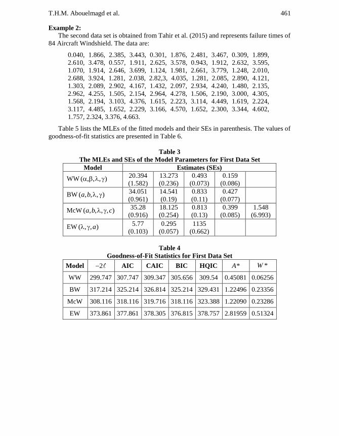
Example 2: The second data set is obtained from Tahir et al. (2015) and represents failure times of

84 Aircraft Windshield. The data are:

0.040, 1.866, 2.385, 3.443, 0.301, 1.876, 2.481, 3.467, 0.309, 1.899,

2.610, 3.478, 0.557, 1.911, 2.625, 3.578, 0.943, 1.912, 2.632, 3.595,

1.070, 1.914, 2.646, 3.699, 1.124, 1.981, 2.661, 3.779, 1.248, 2.010,

2.688, 3.924, 1.281, 2.038, 2.82,3, 4.035, 1.281, 2.085, 2.890, 4.121,

1.303, 2.089, 2.902, 4.167, 1.432, 2.097, 2.934, 4.240, 1.480, 2.135,

2.962, 4.255, 1.505, 2.154, 2.964, 4.278, 1.506, 2.190, 3.000, 4.305,

1.568, 2.194, 3.103, 4.376, 1.615, 2.223, 3.114, 4.449, 1.619, 2.224,

3.117, 4.485, 1.652, 2.229, 3.166, 4.570, 1.652, 2.300, 3.344, 4.602,

1.757, 2.324, 3.376, 4.663.

Table 5 lists the MLEs of the fitted models and their SEs in parenthesis. The values of

goodness-of-fit statistics are presented in Table 6.

Table 3

The MLEs and SEs of the Model Parameters for First Data Set

Model Estimates (SEs)

WW ( , , , ) 20.394

(1.582)

13.273

(0.236)

0.493

(0.073)

0.159

(0.086)

BW ( , , , )a b 34.051

(0.961)

14.541

(0.19)

0.833

(0.11)

0.427

(0.077)

McW ( , , , , )a b c 35.28

(0.916)

18.125

(0.254)

0.813

(0.13)

0.399

(0.085)

1.548

(6.993)

EW ( , , )a 5.77

(0.103)

0.295

(0.057)

1135

(0.662)

Table 4

Goodness-of-Fit Statistics for First Data Set

Model 2 AIC CAIC BIC HQIC *A *W

WW 299.747 307.747 309.347 305.656 309.54 0.45081 0.06256

BW 317.214 325.214 326.814 325.214 329.431 1.22496 0.23356

McW 308.116 318.116 319.716 318.116 323.388 1.22090 0.23286

EW 373.861 377.861 378.305 376.815 378.757 2.81959 0.51324


Table 5

The MLEs and SEs for Second Data Set

Model Estimates (SEs)

WW ( , , , ) 24.862

(1.44)

3.752

(0.298)

0.199

(0.069)

0.545

(0.113)

BW ( , , , )a b 53.874

(2.717)

20.528

(0.278)

1.076

(0.278)

0.231

(0.184)

McW ( , , , , )a b c 51.321

(5.329)

19.762

(0.605)

1.119

(0.48)

0.23

(0.424)

1.525

(38.539)

EW ( , , )a 7.017

(0.134)

0.144

(0.063)

1773

(0.827)

Figure 3: Estimated Densities of the Fitted Models for Data Set 1

Figure 4: Estimated cdfs of for Data Set 1


Table 6

Goodness-of-Fit Statistics for Second Data Set

Model 2 AIC CAIC BIC HQIC *A *W

WW 261.389 269.389 269.895 269.086 273.298 0.65619 0.07529

BW 289.948 297.948 298.455 297.645 301.857 3.34711 0.48715

McW 283.983 293.983 294.752 293.604 298.869 3.33313 0.4847

EW 320.347 326.347 326.647 324.196 326.302 32.74879 7.04167

It is observed, from Table 6, that the WW distribution gives a better fit than other fitted

models. Plots of the histogram, fitted densities and estimated cdfs are displayed in

Figures 5 and 6, respectively.

Figure 5: Estimated pdfs for Data Set 2


Figure 6: Estimated cdfs for Data Set 2

7. CONCLUSIONS

In this paper, we study a four-parameter model, named the Weibull Weibull (WW)

distribution. The WW model is motivated by the wide use of the Weibull distribution in

practice. The WW pdf can be expressed as a mixture of Weibull densities. We derive

explicit expressions for the quantile function, ordinary and incomplete moments,

moments of the residual and reversed residual function, order statistics and Rényi and q-

entropies. The maximum likelihood estimation method is used to estimate the model

parameters. We provide some simulation results to assess the performance of the

proposed model. The practical importance of the WW distribution is demonstrated by

means of two real data sets.

ACKNOWLEDGMENTS

The authors would like to thank the Editor and the five anonymous referees for

carefully reading the article and providing valuable comments which greatly improved

the paper.

REFERENCES

1. Afify, A.Z., Cordeiro, G.M., Ortega, E.M.M., Yousof, H.M. and Butt, N.S. (2016a).

The Four-Parameter Burr XII distribution: properties, Regression Model and

applications. Communications in Statistics-Theory and Methods, forthcoming.

2. Afify, A.Z., Yousof, H.M., Cordeiro, G.M., Ortega, E.M.M. and Nofal, Z.M.,

(2016b). The Weibull Fréchet distribution and its applications. Journal of Applied

Statistics, 43, 2608-2626.

3. Alexander, C., Cordeiro, G.M., Ortega, E.M., Sarabia, J.M. (2012). Generalized beta

generated distributions. Computational Statistics and Data Analysis, 56(6),

1880-1897.


4. Alizadeh, M., Emadi, M., Doostparast, M., Cordeiro, G.M., Ortega, E.M.M., Pescim,

R.R. (2015). Kumaraswamy odd log-logistic family of distributions: Properties and

applications. Hacettepe University Bulletin of Natural Sciences and Engineering

Series B: Mathematics and Statistics. Forthcoming, available at DOI:

10.15672/HJMS.2014418153.

5. Alzaatreh, A., Lee, C. and Famoye, F. (2013). A new method for generating families

of continuous distributions. Metron, 71(1), 63-79. 6. Bourguignon, M., Silva, R.B. and Cordeiro, G.M. (2014). The Weibull-G family of

probability distributions. Journal of Data Science, 12(1), 53-68.

7. Carrasco, J.M., Ortega, E.M. and Cordeiro, G.M. (2008). A Generalized Modified

Weibull Distribution for Lifetime Modeling. Computational Statistics & Data

Analysis, 53(2), 450-462. 8. Cordeiro, G.M. and de Castro, M. (2011). A new family of Generalized Distributions.

Journal of Statistical Computation and Simulation, 81(7), 883-898.

9. Cordeiro, G.M., Alizadeh, M. and Diniz Marinho, P.R. (2016). The type I half-

logistic family of distributions. Journal of Statistical Computation and Simulation,

86(4), 707-728.

10. Cordeiro, G.M., Hashimoto, E.M. and Ortega, E.M.M. (2014). The McDonald

Weibull model. Statistics: A Journal of Theoretical and Applied Statistics, 48(2)

256-278.

11. Cordeiro, G.M., Saboor, A., Khan, M.N., Ozel, G. and Pascoa, M.A. (2016). The

Kumaraswamy exponential-Weibull Distribution: Theory and applications. Hacettepe

Journal of Mathematics and Statistics, 45(4), 1203-1229.

12. Elgarhy, M., Hassan, A.S. and Rashed, M. (2016). Garhy-Generated Family of

Distributions with Application, Mathematical Theory and Modeling, 6, 1-15.

13. Eugene, N., Lee C. and Famoye, F. (2002). Beta-normal distribution and its

applications. Communication in Statistics-Theory Methods, 31, 497-512.

14. Hassan, A.S. and Elgarhy, M., (2016). Kumaraswamy Weibull-Generated Family of

Distributions with Applications. Advances and Applications in Statistics, 48, 205-239.

15. Hassan, A.S. and Hemeda, S.E. (2016). The Additive Weibull-g Family of Probability

Distributions. International Journals of Mathematics and its Applications, 4, 151-164.

16. Hassan, A.S., Elbatal, I. and Hemeda, S.E. (2016). Weibull Quasi Lindley

Distribution and its Statistical Properties with Applications to Lifetime Data.

International Journal of Applied Mathematics and Statistics, 55, 63-80.

17. Hassan, A.S., Elgarhy, M. and Shakil, M. (2017). Type II Half Logistic Family of

Distributions with Applications. Pakistan Journal of Statistics and Operation

Research, 13, 245-264.

18. Lee, C., Famoye, F. and Olumolade, O. (2007). Beta-Weibull distribution: some

properties and applications to censored data. Journal of Modern Applied Statistical

Methods, 6(1), 173-186.

19. Merovci, F. and Elbatal, I. (2015). Weibull rayleigh distribution: Theory and

applications. Applied Mathematics & Information Sciences, 9(4), 2127-2137.

20. Mudholkar, G.S. and Srivastava, D.K. (1993). Exponentiated Weibull family for

analysing bathtub failure rate data. IEEE Transactions on Reliability, 42, 299-302.


21. Mudholkar, G.S., Srivastava, D.K. and Kollia, G.D. (1996). A generalization of the

Weibull distribution with application to the analysis of survival data, Journal of the

American Statistical Association, 91, 1575-1583.

22. Nicholas, M.D. and Padgett, W.J. (2006). A bootstrap control chart for Weibull

percentiles, Quality and Reliability Engineering International, 22, 141-151.

23. Oguntunde, P.E., Balogun, O.S., Okagbue, H.I. and Bishop, S.A. (2015). The

Weibull-Exponential Distribution: Its Properties and Applications. Journal of Applied

Sciences, 15, 1305-1311.

24. Rényi, A. (1961). On measures of entropy and information. In: Proceedings of the 4th

Fourth Berkeley Symposium on Mathematical Statistics and Probability, 547-561.

University of California Press, Berkeley.

25. Tahir, M.H., Cordeiro, G.M., Mansoor, M. and Zubair, M. (2015a). The Weibull-

Lomax Distribution: Properties and Applications. Hacettepe Journal of Mathematics

and Statistics, 44(2), 461-480.

26. Tahir, M.H., Cordeiro, G.M., Alzaatreh, A., Mansoor, M. and Zubair, M. (2016).

A New Weibull-Pareto Distribution: Properties and Applications. Communications in

Statistics-Simulation and Computation, 45(10), 3548-3567.

27. Tahir, M.H., Gauss, M., Cordeiro, Alzaatreh, A.M., Mansoor, M., Zubair and

Alizadeh, M. (2015b). The Weibull-Dagum distribution: properties and applications,

Communication in Statistics-Theory and Methods, 42, 1673-1691.

28. Weibull, W. (1951). A Statistical Distribution Function of wide Applicability. Journal

of Applied Mechanics, 18, 293-297.

29. Xie, M., Tang, Y. and Goh, T.N. (2002). A Modified Weibull extension with bathtub-

shaped failure rate function. Reliability Engineering & System Safety, 76(3), 279-285. 30. Zografos, K. and Balakrishnan, N. (2009). On families of Beta-and Generalized

Gamma-Generated Distributions and Associated Inference. Statistical Methodology,

6(4), 344-362.

pak. j. statist. 2017 vol. 33(6), 449-466 properties of ...6)/33(6)04.pdf · figure 2 displays some...

Documents