paper no. 2650 - usf college of engineeringsagues/documents/nace 13 2650 unexpt corr... ·...

Unexpected Corrosion of Aluminized Steel Pipes in Limestone Backfill

Mersedeh Akhoondan HDR | Schiff

431 West Baseline Road Claremont, CA 91711 U.S.A.

Alberto A. Sagüés

Department of Civil and Environmental Engineering University of South Florida

4202 East Fowler Ave. Tampa, FL 33620 U.S.A.

ABSTRACT (1)

Aluminized steel Type 2 (AST2), ASTM A929, has a ~50 um thick coating with outer and inner layers of commercially pure Al and Al-Fe intermetallic respectively. AST2 culvert and drainage pipes are required to have long service life (e.g. 75 yr) in natural soil and water environments; premature pipe failures incur heavy repair and replacement costs. Performance has been adequate in many service conditions, but unexpected early corrosion of AST2 pipes has been recently observed in some Florida inland locations. A recent event with loss of the coating and local penetration of the substrate, after only ~3 years of service was associated with the use of calcium carbonate-rich (limestone) backfill. Water in contact with limestone and allowed to equilibrate with CO2 in the atmosphere (open system) tends to develop a near neutral pH, compatible with a stable passive film on Al, so experiments were conducted to determine if the aggressive conditions took place otherwise. Simulated field fresh water conditions were created, where water in a limestone filled cell was constantly replenished at a slow rate (representing rainwater), while the pH and conductivity were monitored. Under these conditions, a high, steady state pH > 9 developed that was aggressive to the aluminum passive film. The higher pH was ascribed to the dissolution of limestone in slowly flowing water that is not given enough time for equilibration with atmospheric CO2 (approaching a closed system). Electrochemical impedance measurements indicated the onset of severe corrosion early in the exposure, confirmed by metallographic and SEM observation of loss of coating in extracted AST2 specimens. The Al-Fe intermetallic was much less attacked. The corrosion rate decreased later as a thick corrosion product layer formed. Corrosion mechanisms are discussed. These findings merit consideration in updating specifications for the installation and use of backfill materials for aluminized steel culvert pipes. Key Words: aluminum, steel, coating, corrosion, limestone, backfill, culvert pipe, high pH

(1)

Portions of this paper were included in an earlier publication describing preliminary findings, to be published by ECS Transactions. This paper is a comprehensive description of the investigation with the latest findings.

1

Paper No.

2650

©2013 by NACE International.Requests for permission to publish this manuscript in any form, in part or in whole, must be in writing toNACE International, Publications Division, 1440 South Creek Drive, Houston, Texas 77084.The material presented and the views expressed in this paper are solely those of the author(s) and are not necessarily endorsed by the Association.

INTRODUCTION

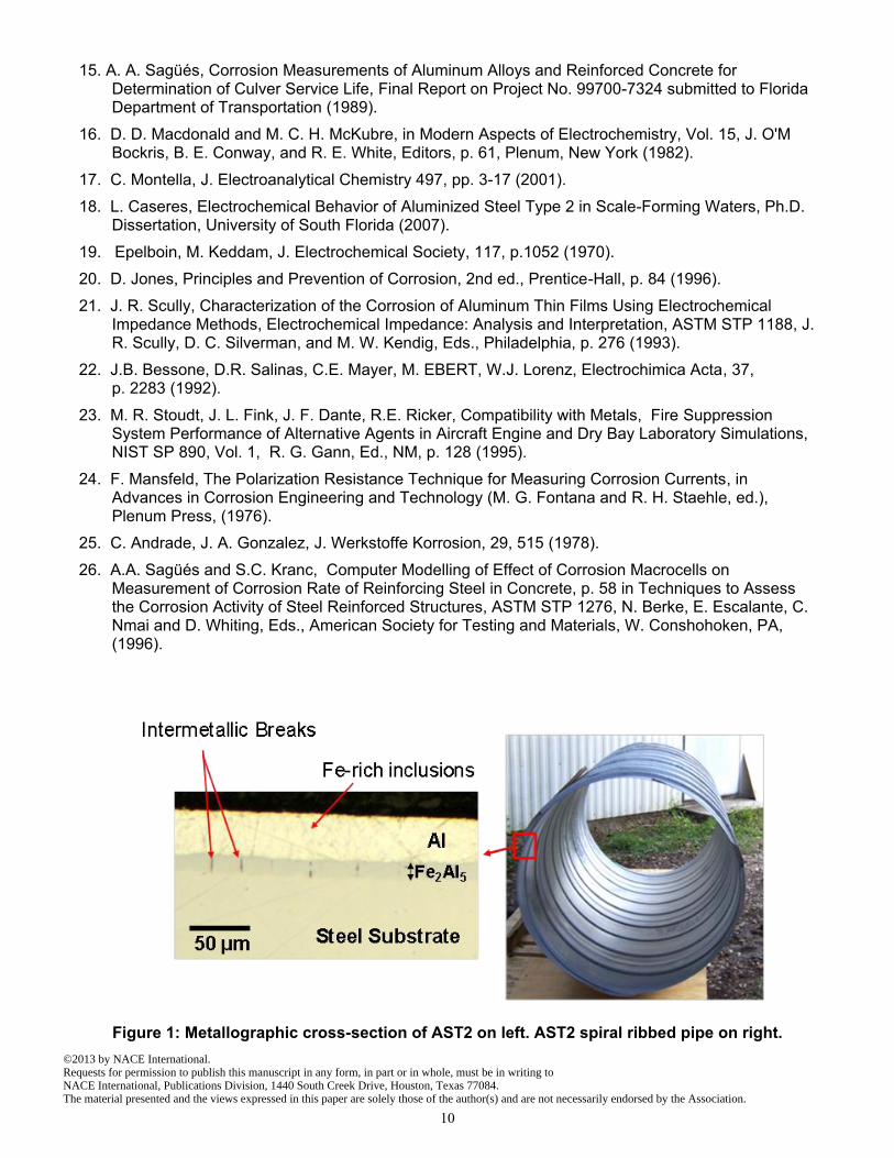
Aluminized steel Type 2 (AST2) is produced as a steel sheet hot-dip coated on both sides with commercially pure aluminum (ASTM(2) A929 and AASHTO(3) M274). The final coating over the carbon steel base is ~50 µm, including a 35 µm thick outer coating having a nearly pure aluminum matrix with

intermetallic precipitates and a 15 m intermetallic inner layer with frequent breaks, as shown in Figure 1. In mild environments, as those commonly found in Florida’s inland waters, the aluminum outer layer naturally forms a stable passive film, which protects aluminum from further corrosion. The main

composition of this film in water is reported as hydragillite, Al2O3.3H2O. 1-2 Hydragillite is

thermodynamically stable in the pH range of about 4 to 8.5 for solute species concentrations in the order of 10-4 M. 3 Beyond this range, the passive film is dissolved as Al3+ in acidic, and AlO2

- (aluminate ion) in basic, environments. 1-2 Upon breakdown of the protective film the coating provides some limited galvanic protection to any exposed steel substrate.4 Culvert and drainage pipes made of AST2 are commonly corrugated or ribbed for greater structural stiffness, and are required to have long service life (e.g. 75 yr) in natural soil and water environments.5 Construction aggregates complying with ASTM C568-96 for bedding and backfill of pipes are often used to provide good structural support. Among these aggregates, crushed limestone (mostly CaCO3) is frequently used for its availability (1.17 billion metric tons production in US in 2009) and cost effectiveness.6 AST2 performance has been adequate in many service conditions, but unexpected early corrosion of AST2 pipes has been recently observed in some inland Florida locations.7 In one particularly severe case, complete penetration of the coating and mild steel substrate, starting from the soil side, took place in only 3 years over a > 10 m long section of pipe that was placed on a limestone backfill. Metallographic cross section of a field sample indicated widespread consumption of the outer aluminum layer, a less affected intermetallic inner layer, and severe localized undercutting attack of the steel substrate. Chemical tests of water in the pipe (in contact with external water through the wall perforations) showed insignificant amount of aggressive ions such as chloride and sulfate at the site. It was speculated for this case that the dissolution of limestone backfill in the soil side water may have generated a high pH environment beyond the regime for stability of the aluminum passive film. A possible objection to that explanation is that water in contact with limestone in an open system, equilibrated with atmospheric CO2, develops only a mildly alkaline pH, typically ~8.3, 8 that is virtually non-aggressive to a passive film on aluminum. However, previous studies on the utilization of limestone contactors for water treatment, 9-10 showed that dissolution of calcium carbonate in a closed system may increase the pH beyond 9. In the case of AST2 pipes in limestone backfill, slowly flowing water (e.g. rain) that is not given enough time for equilibration could approach closed system conditions and result in significant corrosion. Therefore, the objective of this work was to determine whether contact with limestone in flowing water could result in an elevated pH for the rapid corrosion of aluminized steel such as that observed in the field, and to further understand the mechanism of that corrosion. The findings merit consideration to assist in updating specifications for the installation and use of backfill materials for aluminized steel culvert pipes.

EXPERIMENTAL PROCEDURE

Laboratory experiments were conducted using 5 cm by 7.6 cm specimens (total exposed area of ~77 cm2) cut from as-received AST2 gage 16 (1.6 mm thick) flat sheet stock. A contact wire with an

(2)

ASTM International, 100 Barr Harbor Drive, PO Box C700, West Conshohocken, PA, 19428-2959 (3)

American Association of State Highway and Transportation Officials. (AASHTO), 444 N Capitol St. NW - Suite 249 - Washington, DC 20001

2


insulating sheath was either spot welded or soldered to one of the edges. All the edges and wire connections were covered with two-component epoxy which was allowed to set for 24 hrs. Then, the exposed metallic surfaces were degreased with ethanol and stored in a desiccator prior to immersion. The immersion cells (Figure 2) were upright cylinders made of acrylic glass (10 cm internal diameter and 10 cm tall). The lower 8 cm contained ~0.8 kg of limestone crushed to a size between 1 cm and 3 cm, in which the specimen was embedded so its surface was in direct contact with multiple limestone particles. The composition of the limestone was tested in accordance with ASTM C1271 and confirmed to be ~97 wt% CaCO3 which is comparable to commonly reported values for limestone. 11 Before being placed in the cells, the limestone particles were pre-washed with tap water, then DI water and were spread in a tray to dry at room temperature overnight.

The feed water was commercially supplied distilled water of resistivity > 50 k-cm, representing rural rainwater. 12 The feed water was held in a tank that allowed initial equilibration with atmospheric oxygen and CO2. Peristaltic pumps fed the water into each cell at a rate of ~2 liter per day. The water entered the cell at the lower end, ran in contact with the fully immersed specimen and the limestone, and was removed through an opening level to the top of the limestone fill. The chosen flow rate was intended to allow for dissolution of limestone while avoiding excessive introduction of additional CO2 from air into the cell solution, approximating a post-dissolution close system condition. A total of 14 specimens were tested in these flowing conditions. The pH, conductivity, and open circuit potential (EOC) measurements were taken daily. For electrochemical measurements a titanium mesh with mixed metal oxide surface activation was placed around the inner wall of the cell to serve as a counter electrode. A similarly activated titanium rod 3 mm in diameter and 50 mm long was placed parallel to the specimen surface halfway to the counter electrode mesh, to serve as a low impedance temporary reference electrode. 13 It was periodically calibrated against a saturated calomel electrode (SCE). All potentials reported here are in the SCE scale. Electrochemical impedance spectroscopy (EIS) measurements were periodically obtained for 8 of the specimens at the EOC with a Gamry† Ref. 600 potentiostat in the frequency range from 100 kHz to 10 mHz using sinusoidal signals of 10 mV rms amplitude. All tests were conducted at room temperature. After exposure, the specimens were extracted and inspected for crevice corrosion. No crevice corrosion indications were observed in any of the cases. The tests and results for the first ~150 days are presented here. Control specimens were exposed and tested in similar cells where the feed water was allowed to reach atmospheric equilibrium and not replenished.

RESULTS Solution pH In the cells with no flowing water, the pH decayed to < 8.5 after one day and reached terminal values ≤ 8.3 afterwards. These values approximate the expected condition, noted earlier, for water in contact with limestone and equilibrated with atmospheric CO2. Notably, the pH within the flowing water cells was found to have a stable value of ~9.3 starting with the first day of exposure. Computational chemical equilibrium model calculations using the program

MINEQL+†, 14 indicated that the pH for water at 25 oC in contact with solid calcium carbonate, but

without contact with atmospheric CO2 (closed system) would be 9.91. If the water was assumed to be in equilibrium with atmospheric CO2 before, but not after contact with calcium carbonate, the computed result was only slightly smaller, pH = 9.84 indicating that any atmospheric CO2 present in the feed water before entering the cells should not be highly consequential. The pH ~ 9.3 value in the flowing

† Trade name

3


water cells therefore indicates that the conditions tend to approximate those of a closed system, where the interaction with atmospheric CO2 cannot keep pace with the dissolution of limestone in the inflowing water. Corrosion development - physical observations Consistent with the resulting mild conditions, corrosion in the cells with no flowing water was relatively unimportant during the test period and details of those results are addressed later on. In contrast, and as expected from the high pH solution, rapid corrosion of the aluminized coating took place in the flowing water cells. Direct observation of extracted specimens revealed that severe coating damage and surface discoloration took place starting after a short (about two weeks) exposure (Figure 3). SEM observations confirmed severe loss of aluminized coating later on, as illustrated in Figure 4. As shown, the coating loss was rather generalized as opposed to sharply concentrated. The corrosion products consisted mainly of a dense, inner region that took the place of the consumed outer aluminized layer, and a usually thinner and more porous outer region. In the inner corrosion product layer, the Al-Fe intermetallic particles remained embedded and uncorroded, extending from the outer aluminized layer matrix. It noted that pits with some corrosion of the underlying steel were observed after around 150 days of exposure. This paper focuses on the precursors of those events. The subsequent development of strong localized corrosion of the steel substrate should be investigated at length in follow up work. Corrosion development - electrochemical behavior Figure 5, shows the potential evolution for control specimens as well as for the 8 specimens for which EIS measurements were frequently performed. The potential values for no flowing water cells approached a terminal value of ~ - 500 mVSCE. Potential values significantly more positive than ~ - 900 mV SCE are not uncommon for generally passive aluminum in non-aggressive waters. 15 To interpret the EIS data, and estimate the corrosion rate for the Control specimens, a similar approach to Stage I, for flowing water condition, explained later, was used. Estimated corrosion rates were significantly smaller than those in the flowing water cells, as shown in comparative plots later on. For flowing water cells, the EOC initially decreased and reached a minimum (~ -1 VSCE) indicative of highly active aluminum corrosion after about two weeks of exposure (Figure 5). Typical EIS behavior is shown for different exposure times in Figure 6 and Figure 7. The high frequency loop (100 Hz - 100 kHz), only shown for day 1 in Figure 6, reflects water dielectric properties apparent because of the high resistivity of the solution and was omitted in subsequent analysis. The solution resistance corresponded to the real value of the impedance at ~100 Hz. Variations with time of the solution resistance stemmed from minor changes in feed water composition and is not of consequence to the following analysis. The impedance behavior shown in Figures 6-7 and the Eoc evolution shown in Figure 5 make evident the presence of two Stages in the electrochemical evolution of the system. Stage I took place early in the exposure of the specimens (~ first two weeks) and is characterized by rapidly decreasing values of Eoc and an impedance that reaches minimum values after about two weeks. During most of Stage I the impedance diagrams showed two clearly differentiated time constants (Figure 6). Stage I is followed by a subsequent Stage II where the nominal polarization resistance gradually increased, and only one time constant is observed in the impedance diagrams (Figure 7). The assumptions and the approach used to interpret the EIS results to obtain estimates of the corrosion rate prevalent in each of the stages is identified next.

DISCUSSION Interpretation of EIS Data Control specimens and Stage I, flowing water condition: The circuit chosen to simulate the impedance response of EIS data in Stage I for flowing water cells, as well as the entire exposure times of no flowing water cells, is shown in Figure 8 A. The circuit accounts for the impedance response of the electrolyte interface with the aluminum matrix of the outer aluminized coating layer, and of any exposed

4


intermetallic precipitate particles. RSol represents the ohmic solution resistance and Constant Phase Element 1 (CPE1)

(4) represents the combined capacitive behavior of the passive film on the aluminum matrix and the precipitates (the latter being a minor component for the passive behavior and neglected in the following). In a more sophisticated analysis, the film capacitance could be considered to be in series with a double layer capacitance. However, the admittance of a double layer is expected to be significantly greater than that of the passive film; thus, in a series combination, the latter would dominate, and consequently the former is neglected here. 4 The corrosion potential of the passive interfaces is assumed to be the combined mixed potential of the passive anodic dissolution processes and cathodic reactions, such as oxygen reduction, taking place primarily on the intermetallic precipitates present at the surface. Assuming a near-potential independent region (characteristic of passive dissolution) for the anodic reaction on the aluminum matrix or the precipitates, the impedance can be approximated by a resistor with a very large value. 16 The contribution of that component can then be considered negligible on first approximation, given the parallel circuit configuration used. In an attempt to explain the presence of two time constants in the impedance diagram for Stage 1, it is proposed that the cathodic reaction taking place on these precipitates is a two step reaction (with generation of an intermediate adsorbate on the surface) where the overall rate of cathodic reaction depends on the rate of each step (specific to the portion of the surface on which the step takes place), and it also depends on the potential. 4, 16-19. If the potential of the system (assuming it is in a steady state condition) was suddenly altered, the rate of each reaction would experience a sudden change followed by relaxation toward a final new steady state value. The Faradaic impedance behavior of such multi-step reactions has been expressed in terms of components shown in lower branch of the circuit (Figure 8 A). 4,16,18 At high frequencies (immediate potential changes), the impedance of the circuit is given by Resistor R1, since CPE2 acts as a short circuit at those frequency ranges. At low frequencies, CPE2 corresponds to an open circuit, and the overall impedance is the sum of R1 and R2. Thus, R1 is the value of the charge transfer resistance and R1+R2 is the value of the polarization resistance. CPE2, together with R2, determine the characteristic time constant of the relaxation process in between both conditions. It is noted that the value of R2 is a complicated function of the system parameters and not directly associated with the overall rate of the cathodic reaction. Hence, the value of R2 will not be used to estimate the corrosion rate here. However, R1 can be expressed in simpler terms as a function of the overall cathodic reaction rate and the kinetic constants of each of the reacting steps by the following relationship: 16,19

R1 =

Eq (1)

where: n and m, are the number of electrons consumed in each reaction step. As a working assumption, the overall reaction will be considered to correspond to oxygen reduction, with a general expression as O2+2H2O+4e- 4OH-, and formally assigning values of n=m=2 for the charge transacted in each of two consecutive steps as proposed elsewhere. 19 Ic (treated here as a positive number) is the total cathodic current taking place on the intermetallic precipitate surfaces. β 1 and β 2 correspond to the Tafel slopes for each of the reaction steps. For the purpose of this analysis, a Tafel slope value of 120 mV/dec was assumed for each reaction. Such value is customarily used for approximate calculations when the actual values of Tafel slopes are unknown. 20

(4)

The admittance of the CPE is Yo(jω)n where Yo is the pre-exponential admittance term, ω is the angular

frequency, and 0≤n≤14.

5


Inserting the assumed parameter values Eq (1) reduces to:

R1 = 0.052 V / Ic Eq (2)

Since, under open circuit steady state conditions, the total cathodic current is equal to the total anodic current, the value Icorr = 0.052V / R1 provides an estimate of the anodic reaction current, effectively the corrosion current of the system under the above assumptions. If the anodic reaction were uniformly distributed over the specimen surface, the corresponding corrosion current density would be given by icorr = Icorr / A where A= 77 cm2. This issue is addressed in more detail later on. Using the above approach to interpret the EIS data, for all specimens during most of Stage I, the n value obtained for CPE1 was typically ~ 0.9 (thus approaching ideally capacitive behavior with nominal capacitance C ~ Yo sec(1-n) ). Nominal capacitance values for this CPE were in order of 4 uF cm-2 initially and increased with time. Such values are consistent with those expected for the capacitance of naturally formed aluminum passive films. 21-22 An estimate of the nominal thickness (d) of the film during Stage I was made using Eq (3):

d = ε0* ε * A / C Eq (3)

where: ε is the dielectric constant of the passive film (estimated to be ~8), 21 εo is the permittivity of free space (8.85x10-14 F/cm), A is the area of the metal coating (~77cm2), C was the capacitance value obtained from CPE1. The nominal film thickness is plotted as a function of time in Figure 9 for multiple replicate specimens. The initial thicknesses were about 2-3 nm thick, comparable to values reported in previous studies. 21-22 The values decreased with time and reached atomic dimensions (e.g. ~0.2 nm) after about 2 weeks. That condition may be viewed as being indicative of full consumption of the film at that time. Such interpretation is consistent with the concurrent strong drop in nominal polarization values (onset of severe corrosion), lowered EOC (approaching the potential of actively corroding aluminum), and the appearance of a light grey shade on the surface of the specimens at the end of Stage I. Around the transition between Stages I and II, for a short period (~0-5 days, somewhat different for each specimen), the EIS impedance diagrams did not show clearly differentiated semicircles. The fit using the equivalent circuit in Figure 8 A was affected by considerable uncertainty when applied to the EIS data obtained during the transition period; Therefore, an alternative rough estimate of the corrosion rate for the transition period was conducted as follows. First, a nominal polarization resistance, Rpn, was defined for all tests during Stage I by subtracting the solution resistance from the real part of impedance at 10 mHz. Then, the ratio of r = R1/Rpn was calculated for each specimen for each EIS experiment in Stage I that was conducted before the transition period. A linear regression of the value of r as a function of time was performed for each specimen, yielding slope and intercept values for the specimen. The trend lines had comparable parameters, so an average slope and an average intersection were calculated and used as master parameters for the group. The master parameters were then applied to the time corresponding to each of the transition period experiments, which provided an extrapolated value of r for each instance. Then, the Rpn values obtained during the transition period was multiplied by the extrapolated r value to obtain an estimate of R1. That value was then used to obtain the estimate of the corrosion rate using Eq (1).

6


Stage II: The impedance diagrams obtained during Stage II, (Figure 7), differed from those in Stage I. Starting shortly after the onset of Stage II and from then on there was typically only one loop, consisting of a moderately depressed semicircle. The impedance spectrum, concentrating again on frequencies below ~100 Hz for the reasons stated in the Stage I discussion, could be closely approximated by the response of a simple parallel combination of a CPE (CPE3) and a resistor (R3) in series with an ohmic solution resistance element (Figure 8 B). The relatively large value of CPE3 and moderate deviation from ideality (n3 typically ~0.7) obtained from the above analysis were comparable to those often observed for the surface of metals undergoing corrosion in the active state. 4,18 It will be thus assumed that the value of Rp3 represents the polarization resistance of an actively corroding electrode. Following the arguments explained for Stage I, Rp3 can be envisioned as being the parallel combination of two impedance elements, related to the anodic and cathodic processes respectively. For reasons explained next, it will be further assumed that one of the reactions is subject to near complete diffusional control which would result in a very high impedance value at the low frequencies associated with the observed loop. Hence, the contribution of that element can be ignored in the following. Given that the spectrum contains only one identifiable loop, the other reaction can then be speculatively associated with a simple one-step, activation limited reaction with polarization resistance. 18 Using Rp3 values and assuming Tafel slope values of 120 mV/dec, 20 the corrosion current (assuming that the reaction is uniformly distributed over the specimen surface) at this stage was calculated by Eq (4):

Icorr = 0.052V / Rp3 Eq (4)

Estimated corrosion current densities for all specimens exposed to the flowing water condition as well as for control specimens are shown in Figure 10. This graph shows the increasing trend of estimated corrosion density for Stage I and decreasing trend for Stage II for flowing water cells. The results for the control specimens are shown in red dash lines; as noted earlier, these current densities are significantly lower than those estimated for the flowing water condition.

As shown by the metallographic evidence, as aluminum corrodes, the corrosion products are retained in the form of an increasingly deeper penetration layer that, while not highly protective, may act as an increasingly thick barrier to diffusion of one of the reacting species. The subsequent gradual decrease in apparent corrosion current density during Stage II may be interpreted as being the result of the growth of that corrosion product layer. In an attempt to explain that hypothesis, one could imagine a corrosion film that grows inward from the surface of a metal with thickness h that increases with time. As noted earlier, with the exception of a relatively thin outer deposit the penetration did not appear to be in the form of expansive corrosion products so the thickness of the corrosion product layer is on first approximation equal to the thickness of metal lost. The corrosion rate by definition is the change in thickness h with time, dh/dt, which, under a diffusional limitation hypothesis, is proportional to inverse of film thickness (since for thicker film the transport of the species involved in the corrosion process would be slower) 23. Therefore:

dh/dt = K/h Eq (5)

where K is a constant expected to be proportional to the diffusivity of the species involved. Eq (5) can be rewritten as:

h*dh = K*dt Eq (6)

7


It is proposed that before the onset of Stage II, while the oxide film still remained on much of the surface, some extent of non-uniform corrosion was taking place that resulted eventually in the presence of a small but significant corrosion product thickness (hi) at least on some regions of the specimen surface. This occurrence is exemplified by the condition shown in Figure 3, at day 10 (near the end of Stage I). Integrating both sides of Eq (6) with respect to time and thickness yields:

(H2-hi2) = 2K (T-ti) Eq (7) where: H and T are the final cumulative thickness and exposure time respectively and ti is the time at the beginning of Stage II. Taking the logarithm of both sides, Eq (8) indicates a slope of unity for the log-log scale graph of accumulated thickness loss as a function of the time elapsed from the beginning of stage II. log (H2-hi2) = log (T-ti) + log 2K Eq (8)

As a validation test, the corrosion current density values in Figure 10 were used to obtain H and hi parameters, using Faradaic conversion and accounting the time step that for which these corrosion rates took place. The resulting combined graph for the data from all available specimens, up to 150 days of exposure, is presented in Figure 11. The overall slope closely approached the ideal value of 1, in support of the proposed scenario. This outcome was part of the reason for postulating earlier that one of the corrosion reactions was subject to diffusional control in interpreting the impedance data. Comparison of EIS results and metallography Metal loss determined by direct observation of metallographic cross sections of extracted specimens was subject to considerable spatial variability. To obtain a representative indication of direct metal loss, metallographic samples of 2 to 4 random cross sections of each specimen were prepared. For each cross section multiple metallographs at different spots were taken. In each photo frame the average coating loss was measured; then these values were averaged to find an overall penetration thickness for each specimen, with the result shown by red X symbols in Figure 12 where comparison with the metal loss estimated by EIS can be made as well. As can be seen, the EIS estimates and the direct observations show the same general increasing trend with time, and differ numerically on average by not much above a factor of 2 (EIS yielding the lower values). This degree of correlation between electrochemical and direct corrosion assessments is typical of similar studies and reflects both the natural scatter of both diagnostic procedures. 24-25 Furthermore, there is likelihood of some corrosion rate underestimation on the part of the EIS data due to intrinsic limitations resulting from corrosion localization which may have occurred during Stage I as indicated earlier.26 Consequently, both methods

indicate an average loss of aluminized coating in the order of several m after exposure times of only

1-3 months. Considering that the total outer aluminized layer is only about 35 m thick, and that the coating loss showed large spatial variability in the cross sections examined, it is likely that penetration of the coating could take place after only a few years of service at multiple locations when a large surface area of aluminized steel (eg. many m2 as was the case in the field) is exposed to limestone backfill. Moreover, in the case of steel substrate exposure due to occurrence of pits, after initiation of corrosion (shown in Figure 3 for 150 days), the rate of the cathodic reaction, and as a result the overall rate of corrosion, is expected to be significantly enhanced. Such phenomena may significantly increase the rate of coating loss, at least locally, and therefore reduce the service life of the pipe.

8


CONCLUSIONS

The findings suggest the overall corrosion progression in flowing water summarized in Figure 13. During Stage I the passive film on the outer layer of the aluminized coating is consumed by interaction with the high pH generated by dissolution of limestone under near-closed system conditions. After 1-2 weeks the film is completely consumed and active corrosion of the aluminum begins (Stage II) at a high rate. Corrosion products remain in place and transport limitation of one or more of the species responsible for the rate of corrosion ensues in an increasingly thick film. Nevertheless, after several months of exposure a significant fraction of the aluminized coating had been consumed. Aluminate inclusions, and the inner aluminized layer, are less attacked. Corrosion of the underlying carbon steel, not addressed in this paper, is expected to take place at a later age, but the observed attack of the aluminized coating in such short time portends a dramatic reduction in the life expectancy of the pipe compared to the desired performance. The results thus provide an explanation for the early damage observed in the field.

ACKNOWLEDGEMENTS

This investigation was supported by the Florida Department of Transportation. The opinions, findings and conclusions expressed in this publication are those of the authors and not necessarily those of the sponsoring agencies.

REFERENCES

1. J.R. Davis, Corrosion of Aluminum and Aluminum Alloys, ASM International, OH, p. 26 (2000).

2. K.A. Lucas and H. Clarke, Corrosion of Aluminum-Based Metal Matrix Composites, Research Studies Press LTD., NY, p. 25 (1993).

3. M. Pourbaix, Lectures on Electrochemical Corrosion, NACE International, Texas, p. 146 (1995).

4. L. Caseres, A.A. Sagüés, Corrosion of Aluminized Steel in Scale Forming Waters, Paper No. 05348, Corrosion/2005, NACE International, Houston, TX (2005).

5. W.D. Cerlanek, R.G. Powers, Drainage Culvert Service Life Performance and Estimation, State of Florida Department of Transportation, Report No. 93-4A (1993).

6. R. L. Virta, 2009 Minerals Yearbook, U.S. Geological Survey (2010).

7. A. A. Sagüés, N. D. Poor, L. Cáseres, M. Akhoondan, Development of a Rational Method for Predicting Corrosion of Metals in Soils and Waters, Final Report on Project No. BD497 submitted to Florida Department of Transportation (2009). http://www.dot.state.fl.us/research-center/

8. V. L. Snoeyink, D. Jenkins, Water Chemistry, John Wiely& Sons, NY, p. 287 (1980).

9. R.D. Letterman, Limestone Contactors for Corrosion Control in Small Water Supply Systems, Final Report submitted to the U.S. Environmental Protection Agency, Drinking Water Research, MERL, OH (1983).

10. R. D. Letterman, C. T. Driscoll, M. Hadad, J. Environmental Engineering, 117, p. 339 (1991).

11. R. B. Boynton, Chemistry and Technology of Lime and Limestone, John Wiley & Sons, NY (1980).

12. R. Sequeira, F. Lung, Atmospheric Environment, 29, p. 3221 (1995).

13. P. Castro, A.A. Sagüés, E.I. Moreno, L. Maldonado, J. Genesca, Corrosion, 52, p. 609 (1996).

14. W. D. Schecher, D. C. McAvory, MINEQL+: A Chemical Equlibrium Modeling System, Environmental Research Software, Version 4.6 for Windows (2003).

9


15. A. A. Sagüés, Corrosion Measurements of Aluminum Alloys and Reinforced Concrete for Determination of Culver Service Life, Final Report on Project No. 99700-7324 submitted to Florida Department of Transportation (1989).

16. D. D. Macdonald and M. C. H. McKubre, in Modern Aspects of Electrochemistry, Vol. 15, J. O'M Bockris, B. E. Conway, and R. E. White, Editors, p. 61, Plenum, New York (1982).

17. C. Montella, J. Electroanalytical Chemistry 497, pp. 3-17 (2001).

18. L. Caseres, Electrochemical Behavior of Aluminized Steel Type 2 in Scale-Forming Waters, Ph.D. Dissertation, University of South Florida (2007).

19. Epelboin, M. Keddam, J. Electrochemical Society, 117, p.1052 (1970).

20. D. Jones, Principles and Prevention of Corrosion, 2nd ed., Prentice-Hall, p. 84 (1996).

21. J. R. Scully, Characterization of the Corrosion of Aluminum Thin Films Using Electrochemical Impedance Methods, Electrochemical Impedance: Analysis and Interpretation, ASTM STP 1188, J. R. Scully, D. C. Silverman, and M. W. Kendig, Eds., Philadelphia, p. 276 (1993).

22. J.B. Bessone, D.R. Salinas, C.E. Mayer, M. EBERT, W.J. Lorenz, Electrochimica Acta, 37, p. 2283 (1992).

23. M. R. Stoudt, J. L. Fink, J. F. Dante, R.E. Ricker, Compatibility with Metals, Fire Suppression System Performance of Alternative Agents in Aircraft Engine and Dry Bay Laboratory Simulations, NIST SP 890, Vol. 1, R. G. Gann, Ed., NM, p. 128 (1995).

24. F. Mansfeld, The Polarization Resistance Technique for Measuring Corrosion Currents, in Advances in Corrosion Engineering and Technology (M. G. Fontana and R. H. Staehle, ed.), Plenum Press, (1976).

25. C. Andrade, J. A. Gonzalez, J. Werkstoffe Korrosion, 29, 515 (1978).

26. A.A. Sagüés and S.C. Kranc, Computer Modelling of Effect of Corrosion Macrocells on Measurement of Corrosion Rate of Reinforcing Steel in Concrete, p. 58 in Techniques to Assess the Corrosion Activity of Steel Reinforced Structures, ASTM STP 1276, N. Berke, E. Escalante, C. Nmai and D. Whiting, Eds., American Society for Testing and Materials, W. Conshohoken, PA, (1996).

Figure 1: Metallographic cross-section of AST2 on left. AST2 spiral ribbed pipe on right.

10


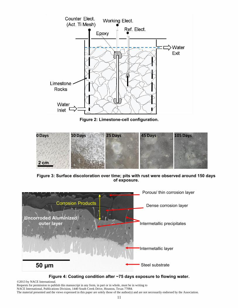
Figure 2: Limestone-cell configuration.

Figure 3: Surface discoloration over time; pits with rust were observed around 150 days

of exposure.

Figure 4: Coating condition after ~75 days exposure to flowing water.

0 Days 10 Days 25 Days 45 Days

2 cm

105 Days

50 µm

Dense corrosion layer

Intermetallic precipitates

Intermetallic layer

Steel substrate

Porous/ thin corrosion layer

Corrosion Products

Uncorroded Aluminized

outer layer

11


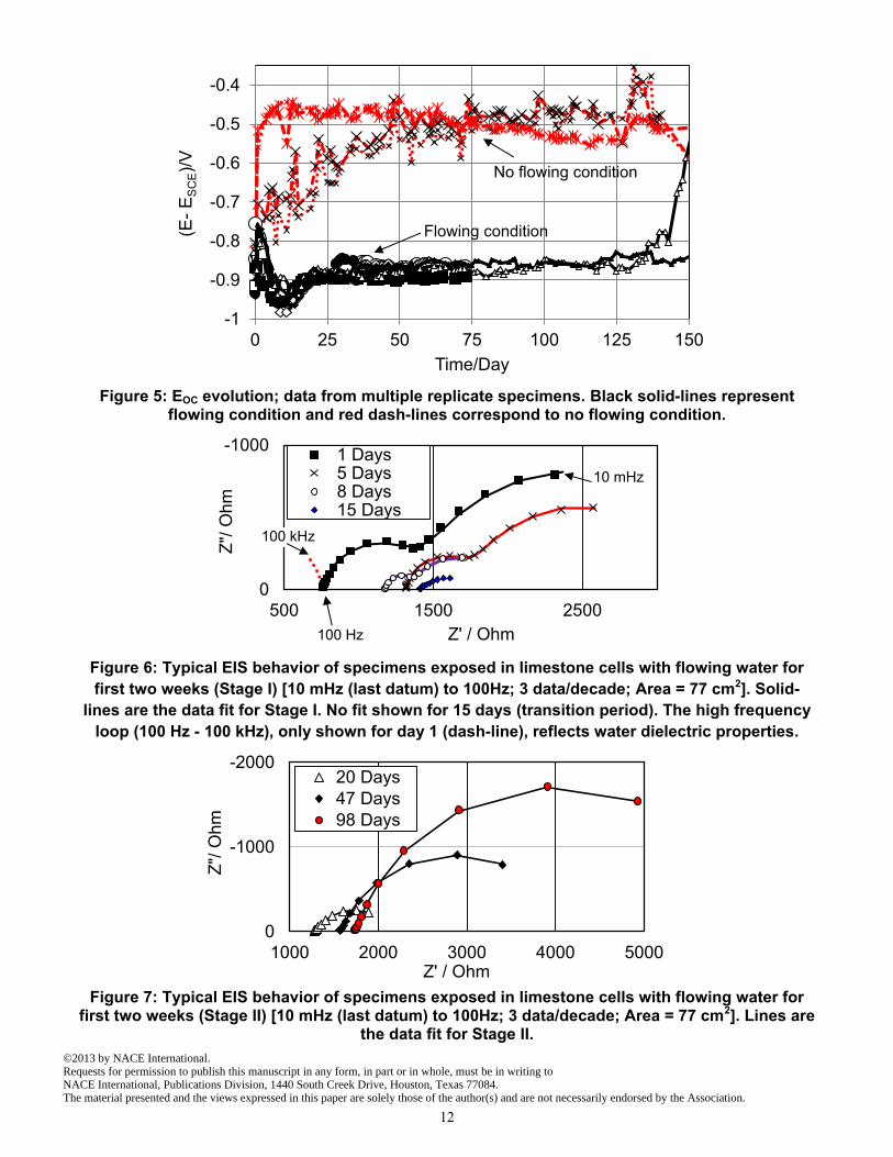
Figure 5: EOC evolution; data from multiple replicate specimens. Black solid-lines represent flowing condition and red dash-lines correspond to no flowing condition.

Figure 6: Typical EIS behavior of specimens exposed in limestone cells with flowing water for

first two weeks (Stage I) [10 mHz (last datum) to 100Hz; 3 data/decade; Area = 77 cm2]. Solid-

lines are the data fit for Stage I. No fit shown for 15 days (transition period). The high frequency

loop (100 Hz - 100 kHz), only shown for day 1 (dash-line), reflects water dielectric properties.

Figure 7: Typical EIS behavior of specimens exposed in limestone cells with flowing water for

first two weeks (Stage II) [10 mHz (last datum) to 100Hz; 3 data/decade; Area = 77 cm2]. Lines are the data fit for Stage II.

-1

-0.9

-0.8

-0.7

-0.6

-0.5

-0.4

0 25 50 75 100 125 150

(E-

ES

CE)/

V

Time/Day

Flowing condition

-1000

0

500 1500 2500

Z"/

Ohm

Z' / Ohm

1 Days5 Days8 Days15 Days

100 kHz

100 Hz

10 mHz

-2000

-1000

0

1000 2000 3000 4000 5000

Z"/

Ohm

Z' / Ohm

20 Days

47 Days

98 Days

No flowing condition

12


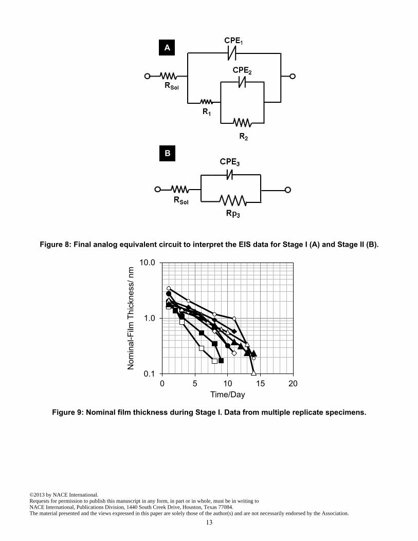
Figure 8: Final analog equivalent circuit to interpret the EIS data for Stage I (A) and Stage II (B).

Figure 9: Nominal film thickness during Stage I. Data from multiple replicate specimens.

0.1

1.0

10.0

0 5 10 15 20

Nom

inal-F

ilm T

hic

kness/ nm

Time/Day

A

B

13


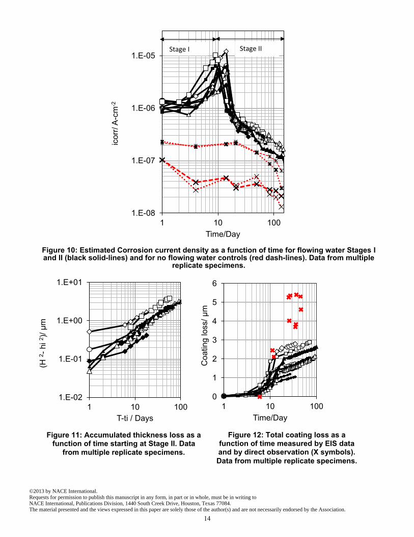
Figure 10: Estimated Corrosion current density as a function of time for flowing water Stages I and II (black solid-lines) and for no flowing water controls (red dash-lines). Data from multiple

replicate specimens.

1.E-08

1.E-07

1.E-06

1.E-05

1 10 100

icorr

/ A

-cm

-2

Time/Day

Stage II Stage I

1.E-02

1.E-01

1.E+00

1.E+01

1 10 100

(H 2

- hi

2)/

µm

T-ti / Days

0

1

2

3

4

5

6

1 10 100

Coating loss/

µm

Time/Day

Figure 11: Accumulated thickness loss as a function of time starting at Stage II. Data

from multiple replicate specimens.

Figure 12: Total coating loss as a function of time measured by EIS data and by direct observation (X symbols).

Data from multiple replicate specimens.

14


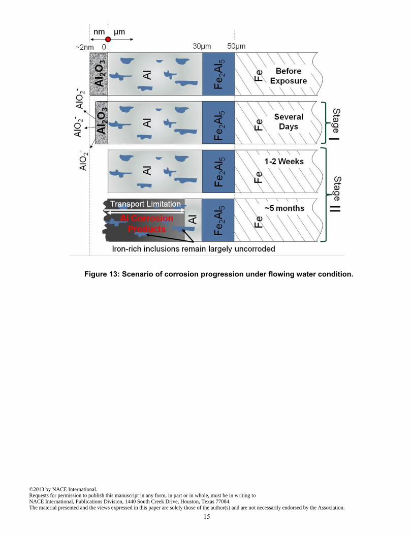
Figure 13: Scenario of corrosion progression under flowing water condition.

15


paper no. 2650 - usf college of engineeringsagues/documents/nace 13 2650 unexpt corr... ·...

Documents