parallel computing with r - louisiana state university€¦ · · 2017-11-01parallel computing...

Parallel Computing with R

Le YanHPC @ LSU

11/1/2017 HPC training series Fall 2017

Parallel Computing: Why?

• Getting results faster– Running in parallel may speed up the time to reach solution

• Dealing with bigger data sets– Running in parallel may allow you to use more memory than that available on a single computer

11/1/2017 HPC training series Fall 2017 1

Example: Moving 200 boxes by 1 person vs. 10 people

Example: Moving a grand piano by 1 person vs. 10 people

Parallel Computing: How?• Identify a group of workers

– For sake of simplicity we will use worker/process/thread interchangeably

• Divide the workload into chunks• Assign one chunk or a number of chunks to each worker

• Each worker processes its own assignment in parallel with other workers


Parallel Computing: Requirements• Hardware: modern computers are equipped with more than one CPU core and are capable of processing workloads in parallel– Your laptop/desktop/workstation has many cores– HPC clusters is composed of many nodes (servers), each of which has many cores

• Software: many software packages are aware of parallel hardware and are capable of coordinating workload processing among workers



• Base R is single‐threaded, i.e. not parallel– Regardless how many cores are available, R can only use one of them



• Base R is single‐threaded, i.e. not parallel– Regardless how many cores are available, R can only use one of them


The goal of this training is to show how to use some R packages to achieve parallel processing

Where We Are with Base R


……

Login node

Node Node Node Node

QB2 Cluster

Cluster = multiple nodes (servers) x multiple cores per node

CPU core

R

What We Want to Achieve


……

Login node

Node Node Node Node

QB2 Cluster

Cluster = multiple nodes (servers) x multiple cores per node

CPU core

R R

R R

R R

R R

R R

R R

R R

R R

R R

R R

R R

R R

Parallel Computing: Caveats

• Using more workers does not always make your program run faster

• Efficiency of parallel programs– Low efficiency means idle workers and vice versa– Defined as speedup divided by number of workers

• 4 workers, 3x speedup, efficiency = 3/4 = 75%• 8 workers, 4x speedup, efficiency = 4/8 = 50%

– Usually decrease with increasing number of workers


Example: Moving 200 boxes by 200 people vs. 1,000 people

Is Parallel Computing for You?


No

No

Don’t bother, e.g. it is perhaps not wise to spend weeks to parallelize a program that finishes in 30 seconds;

Don’t bother, e.g. not much we can do in R if the target R function is written in C or Fortran;

Is your code parallelizable?

Does your code run slow?

Is your code parallel already?

Yes Some R functions utilize parallel numerical libraries – they are implicitly parallel already

Yes

Yes

No

Try parallelization

Implicit Parallelization

• Some functions in R can call parallel numerical libraries– On LONI and LSU HPC clusters this is the multi‐threaded Intel MKL library

–Mostly linear algebraic and related functions• Example: linear regression, matrix decomposition, computing inverse and determinant of a matrix



Cpu0 : 0.0%us, 0.0%sy, 0.0%ni,100.0%id, 0.0%wa, 0.0%hi, 0.0%si, 0.0%stCpu1 : 97.7%us, 2.3%sy, 0.0%ni, 0.0%id, 0.0%wa, 0.0%hi, 0.0%si, 0.0%stCpu2 : 0.0%us, 0.0%sy, 0.0%ni,100.0%id, 0.0%wa, 0.0%hi, 0.0%si, 0.0%stCpu3 : 0.0%us, 0.0%sy, 0.0%ni,100.0%id, 0.0%wa, 0.0%hi, 0.0%si, 0.0%stCpu4 : 0.0%us, 0.0%sy, 0.0%ni,100.0%id, 0.0%wa, 0.0%hi, 0.0%si, 0.0%stCpu5 : 0.0%us, 0.0%sy, 0.0%ni,100.0%id, 0.0%wa, 0.0%hi, 0.0%si, 0.0%stCpu6 : 0.0%us, 0.0%sy, 0.0%ni,100.0%id, 0.0%wa, 0.0%hi, 0.0%si, 0.0%stCpu7 : 0.0%us, 0.0%sy, 0.0%ni,100.0%id, 0.0%wa, 0.0%hi, 0.0%si, 0.0%stCpu8 : 0.0%us, 0.0%sy, 0.0%ni,100.0%id, 0.0%wa, 0.0%hi, 0.0%si, 0.0%stCpu9 : 0.0%us, 0.0%sy, 0.0%ni,100.0%id, 0.0%wa, 0.0%hi, 0.0%si, 0.0%st……Cpu17 : 0.0%us, 0.0%sy, 0.0%ni,100.0%id, 0.0%wa, 0.0%hi, 0.0%si, 0.0%stCpu18 : 0.0%us, 0.0%sy, 0.0%ni,100.0%id, 0.0%wa, 0.0%hi, 0.0%si, 0.0%stCpu19 : 0.0%us, 0.0%sy, 0.0%ni,100.0%id, 0.0%wa, 0.0%hi, 0.0%si, 0.0%stMem: 65876884k total, 9204212k used, 56672672k free, 77028k buffersSwap: 134217724k total, 14324k used, 134203400k free, 5302204k cached

PID USER PR NI VIRT RES SHR S %CPU %MEM TIME+ COMMAND114903 lyan1 20 0 1022m 760m 6664 R 99.9 1.2 0:06.51 R

R running on one node of the QB2 cluster:20 cores total, 1 busy, 19 idle

# Matrix creation and random number generation # are NOT implicitly parallel# Matrix inversion is implicitly parallel # Each node has 20 cores

# Only 1 out 20 cores is busy when running# this lineA <- matrix(rnorm(10000*10000),10000,10000)Ainv <- solve(A)


Cpu0 : 99.7%us, 0.3%sy, 0.0%ni, 0.0%id, 0.0%wa, 0.0%hi, 0.0%si, 0.0%stCpu1 :100.0%us, 0.0%sy, 0.0%ni, 0.0%id, 0.0%wa, 0.0%hi, 0.0%si, 0.0%stCpu2 :100.0%us, 0.0%sy, 0.0%ni, 0.0%id, 0.0%wa, 0.0%hi, 0.0%si, 0.0%stCpu3 : 99.3%us, 0.3%sy, 0.0%ni, 0.0%id, 0.0%wa, 0.0%hi, 0.3%si, 0.0%stCpu4 : 99.7%us, 0.3%sy, 0.0%ni, 0.0%id, 0.0%wa, 0.0%hi, 0.0%si, 0.0%stCpu5 : 99.7%us, 0.3%sy, 0.0%ni, 0.0%id, 0.0%wa, 0.0%hi, 0.0%si, 0.0%stCpu6 : 99.7%us, 0.3%sy, 0.0%ni, 0.0%id, 0.0%wa, 0.0%hi, 0.0%si, 0.0%stCpu7 : 99.7%us, 0.3%sy, 0.0%ni, 0.0%id, 0.0%wa, 0.0%hi, 0.0%si, 0.0%stCpu8 :100.0%us, 0.0%sy, 0.0%ni, 0.0%id, 0.0%wa, 0.0%hi, 0.0%si, 0.0%stCpu9 : 99.7%us, 0.3%sy, 0.0%ni, 0.0%id, 0.0%wa, 0.0%hi, 0.0%si, 0.0%stCpu10 : 99.3%us, 0.3%sy, 0.0%ni, 0.3%id, 0.0%wa, 0.0%hi, 0.0%si, 0.0%st……Cpu16 : 99.7%us, 0.0%sy, 0.0%ni, 0.3%id, 0.0%wa, 0.0%hi, 0.0%si, 0.0%stCpu17 : 99.7%us, 0.3%sy, 0.0%ni, 0.0%id, 0.0%wa, 0.0%hi, 0.0%si, 0.0%stCpu18 : 99.7%us, 0.0%sy, 0.0%ni, 0.3%id, 0.0%wa, 0.0%hi, 0.0%si, 0.0%stCpu19 :100.0%us, 0.0%sy, 0.0%ni, 0.0%id, 0.0%wa, 0.0%hi, 0.0%si, 0.0%stMem: 65876884k total, 11968768k used, 53908116k free, 77208k buffersSwap: 134217724k total, 14324k used, 134203400k free, 5307564k cached

PID USER PR NI VIRT RES SHR S %CPU %MEM TIME+ COMMAND115515 lyan1 20 0 5025m 3.4g 8392 R 1996.5 5.4 1:31.54 R

# Matrix creation and random number generation # are NOT implicitly parallel# Matrix inversion is implicitly parallel # Each node has 20 cores

A <- matrix(rnorm(10000*10000),10000,10000)# 20 out 20 cores are busy when running# this lineAinv <- solve(A)

R running on one node of the QB2 cluster:20 cores total, 20 busy, 0 idle

Know Your R Program• Before starting writing programs, you need to be able

to answer these questions– How do I know the program runs faster after parallelization?

– Which part of my code slows the execution down (the most)?

• First step in parallelization: performance analysis– Purpose: know which part takes how long, and locate the “hotspot” first

– Two most frequent used methods in R• system.time()• rprof() and summaryRprof()


system.time()


## Output from system.time() function## User: time spent in user-mode## System: time spent in kernel (I/O etc.)## Elapsed: wall clock time

## Usage: system.time(<code segment>)

system.time({

A <- matrix(rnorm(10000*10000),10000,10000)Ainv <- solve(A)

})user system elapsed

156.582 0.948 16.325

How much wall clock time it takes ‐ perhaps the most important metric

system.time()


[lyan1@qb032 R]$ cat inv_st.R

print("Matrix creation:")system.time({A <- matrix(rnorm(10000*10000),10000,10000)})

print("Matrix inversion:")system.time({Ainv <- solve(A)})

Measure the execution times of different functions

[lyan1@qb032 R]$ Rscript inv_st.R

[1] "Matrix creation:"user system elapsed7.437 0.278 7.711

[1] "Matrix inversion:"user system elapsed

149.092 0.768 9.417

Note the huge discrepancy between “user” and “elapsed” – it is an indication of implicit parallelization

Code Output

rprof() and summaryRprof()


[lyan1@qb032 R]$ cat inv_prof.R

Rprof()A <- matrix(rnorm(10000*10000),10000,10000)Ainv <- solve(A)Rprof(NULL)summaryRprof()

Start profiling

End profiling

Print profiling result

rprof() and summaryRprof()


[lyan1@qb032 R]$ Rscript inv_prof.R

$by.selfself.time self.pct total.time total.pct

"solve.default" 153.36 95.09 153.58 95.23".External" 6.68 4.14 6.68 4.14"matrix" 1.02 0.63 7.70 4.77"diag" 0.22 0.14 0.22 0.14

$by.totaltotal.time total.pct self.time self.pct

"solve.default" 153.58 95.23 153.36 95.09"solve" 153.58 95.23 0.00 0.00"matrix" 7.70 4.77 1.02 0.63".External" 6.68 4.14 6.68 4.14"rnorm" 6.68 4.14 0.00 0.00"diag" 0.22 0.14 0.22 0.14

How much time is spent in this function itself

How much time is spent in this function and the functions it calls

Writing Parallel R Code –parallel Package

• Introduced in R 2.14.1• Integrated previous multicore and snowpackages

• Coarse‐grained parallelization– Suit for the chunks of computation are unrelated and do not need to communicate

• Two ways of using parallel packages– mc*apply function– for loop with %dopar%

• Need foreach and doParallel packages


Function mclapply

• Parallelized version of the lapply function– Similar syntax with mc.cores indicates how many cores/workers to use

– Return a list of the same length as X, each element of which is the result of applying ‘FUN’ to the corresponding element of X

• Can use all cores on one node– But not on multiple nodes


mclapply(X, FUN, mc.cores = <number of cores>, …)

R R

R R

R R

R R

R

mclapply


# Quadratic Equation: a*x^2 + b*x + c = 0solve.quad.eq <- function(a, b, c){# Return solutionsx.delta <- sqrt(b*b - 4*a*c)x1 <- (-b + x.delta)/(2*a)x2 <- (-b - x.delta)/(2*a)

return(c(x1, x2))}

len <- 1e7a <- runif(len, -10, 10); b <- runif(len, -10, 10); c <- runif(len, -10, 10)

#Serial: lapplyres1.s <- lapply(1:len, FUN = function(x) { solve.quad.eq(a[x], b[x], c[x])})

#Parallel: mclapply with 4 coreslibrary(parallel)res1.p <- mclapply(1:len,

FUN = function(x) { solve.quad.eq(a[x], b[x], c[x]) },mc.cores = 4)

Function solve.quad.eqInput: three coefficients of a quadratic equationOutput: solutions of the quadratic equation

Create 10 million sets of randomly generated coefficients

lapply function: call the solve.quad.eq function for each set of coefficients

mclapply function: same arguments with one extra: mc.cores



return(c(x1, x2))}









> system.time(+res1.s <- lapply(1:len, FUN = function(x) { solve.quad.eq(a[x], b[x], c[x])}))

user system elapsed358.878 0.375 359.046> system.time(+ res1.p <- mclapply(1:len,+ FUN = function(x) { solve.quad.eq(a[x], b[x], c[x]) },+ mc.cores = 4)+ )

user system elapsed11.098 0.342 81.581



return(c(x1, x2))}









> system.time(+res1.s <- lapply(1:len, FUN = function(x) { solve.quad.eq(a[x], b[x], c[x])}))

user system elapsed358.878 0.375 359.046> system.time(+ res1.p <- mclapply(1:len,+ FUN = function(x) { solve.quad.eq(a[x], b[x], c[x]) },+ mc.cores = 4)+ )


It’s always a good idea to check the efficiency of a parallel program:

Speedup = 359.046/81.581 = 4.40Efficiency = 4.40/4 = 110% (!)

%dopar%

• From doParallel package– On top of packages parallel, foreach, iterator

• Purpose: parallelize a for loop• Can run on multiple nodes


R R

R R

R R

R R

R

%dopar%

R R

R R

R R

R R

R R

R R

R R

R R

%dopar%

• Steps– Create a cluster of workers (makeCluster)– Register the cluster (registerDoParallel)– Process the for loop in parallel (foreach … %dopar%)

– Stop the cluster (stopCluster)


%dopar%: On A Single Node


# Parallel version with %dopar%

# Step 1: Create a cluster of 4 workerscl <- makeCluster(4)

# Step 2: Register the clusterregisterDoParallel(cl)

# Step 3: Process the loopls <- foreach(icount(iters)) %dopar% {

to.ls<-rnorm(1e6)to.ls<-summary(to.ls)

}

# Step 4: Stop the clusterstopCluster(cl)

# Workload:# Create 1,000 random samples, each with # 1,000,000 observations from a standard # normal distribution, then take a # summary for each sample.

iters <- 1000

# Sequential versionfor (i in 1:iters) {

to.ls <- rnorm(1e6)to.ls <- summary(to.ls)

}

%dopar%: On A Single Node





# Step 3: Process the loopls<-foreach(icount(iters)) %dopar% {


}



iters <- 1000



}

# Sequentialsystem.time(for (i in 1:iters) {


})


# Parallel with 4 coressystem.time({cl <- makeCluster(4)registerDoParallel(cl)ls<-foreach(icount(iters)) %dopar% {


}stopCluster(cl)})


%dopar%: One Single Node





# Step 3: Process the loopls<-foreach(icount(iters)) %dopar% {


}



iters <- 1000



}

# Sequentialsystem.time(for (i in 1:iters) {


})


# Parallel with 4 coressystem.time({cl <- makeCluster(4)registerDoParallel(cl)ls<-foreach(icount(iters)) %dopar% {


}stopCluster(cl)})


Speedup = 63.739/17.738 = 3.59Efficiency = 3.59/4 = 90%

makeCluster()

• We specify how many workers to use• On the same node:

• On multiple nodes:

– Example: create 4 workers, 2 on qb101 and 2 on qb102


cl <- makeCluster(<number of workers>)

cl <- makeCluster(<list of hostnames>)

cl <- makeCluster(c(“qb101”,”qb101”,”qb102”,”qb102”))

%dopar%: Multiple Nodes on QB2 Cluster


# Read all host nameshosts <-as.vector(unique(read.table(Sys.getenv("PBS_NODEFILE"),stringsAsFactors=F))[,1])# Count number of hostsnh <- length(hosts)# Use 4 workersnc <- 4

# Make a cluster on multiple nodescl <- makeCluster(rep(hosts , each = nc/nh))

registerDoParallel(cl)

ls<-foreach(icount(iters)) %dopar% {


}

stopCluster(cl)

Same steps for the rest of the code:‐ Make a cluster‐ Register the cluster‐ Process loop with %dopar%‐ Stop the cluster

Get the host names of the nodes

Running Parallel R Codes

• Now we have a R code that can run in parallel • So the next question is:

– How do we know how many workers we should we run it with?• The more the better (faster)?


Running Parallel R Codes

• Now we have a R code that can run in parallel • So the next question is:

– How do we know how many workers we should we run it with?• The more the better (faster)?


The answer is: scaling test (trial and error)


cl <- makePSOCKcluster(rep(hosts , each = clusterSize[i]/nh))registerDoParallel(cl)

t <- system.time(ls <- foreach(icount(iters)) %dopar% { to.ls <- rnorm(1e6)to.ls <- summary(to.ls)}

)

stopCluster(cl)

Nothing is returned, so chunks of the workload are independent of each other


ls <- foreach(icount(iters)) %dopar% {to.ls<-rnorm(1e6)to.ls<-summary(to.ls)

}

On one node (20 cores total)

On two nodes (40 cores total)

Ideal behavior

We call this relationship between the number of workers and run time the “scaling behavior”.


ls <- foreach(icount(iters)) %dopar% {to.ls<-rnorm(1e6)to.ls<-summary(to.ls)

}



Ideal behavior

Observations:‐ Deviation from ideal behavior should be

expected;‐ Number of workers can differ from number

of cores, but it doesn’t make sense to have more workers than the number of cores;

‐ More is not necessarily faster, and could be slower;


res2.p <- foreach(i=1:core, .combine='rbind') %dopar%{

# local data for resultsres <- matrix(0, nrow=chunk.size, ncol=2)for(x in ((i-1)*chunk.size+1):(i*chunk.size)) {

res[x - (i-1)*chunk.size,] <- solve.quad.eq(a[x], b[x], c[x])}# return local resultsres

}

The results from each chunk are aggregated into “res2.p”, so chunks of the workload are independent




Ideal behavior




Ideal behavior

Observations:‐ If there is data dependency, performance

deteriorates faster (compared to cases where there is none);

‐ Performance deteriorates faster when some workers on one node and some on the other;

What we have learned about parallel (R) codes

• With increasing number of workers, efficiency decreases, and eventually adding more workers slows it down

• Best scaling behaviors are typically found with codes with no data dependency (we call it “embarrassingly parallel”)

• With this in mind, when developing our codes, we should reduce data dependency as much as possible


How Many Workers to Use


If there is no constraint, minimize the wall clock time

Sometimes our goal should be to maximize efficiency

Summary: Steps of Developing Parallel (R) Codes• Step 1: Analyze performance

– Find “hot spots” – parallelizable code segments that slow down the execution the most

• Step 2: Parallelize code segments• Step 3: Run scaling tests

– How do efficiency and run time change with increasing number of workers?

– What are the optimal number of workers?• Step 4: Is the code fast enough?

– If yes, stop developing (for now) and move on to production runs;

– If no, go back to step 1 and start another iteration.


Memory Management

• Replica of data objects could be created for every worker– Memory usage would increase with the number of workers

• R does not necessarily clean them up even if you close the cluster– Need to monitor memory footprint closely– The Rprof function is capable of memory profiling as well






}

PID USER PR NI VIRT RES SHR S %CPU %MEM TIME+ COMMAND87483 lyan1 20 0 539m 314m 6692 R 100.0 0.5 0:02.05 R87492 lyan1 20 0 539m 314m 6692 R 100.0 0.5 0:02.05 R87465 lyan1 20 0 539m 314m 6692 R 99.4 0.5 0:02.04 R87474 lyan1 20 0 539m 314m 6692 R 99.4 0.5 0:02.05 R

With 4 workers:Memory = 314*4 = 1256 MB





}

PID USER PR NI VIRT RES SHR S %CPU %MEM TIME+ COMMAND87514 lyan1 20 0 501m 276m 6692 R 99.8 0.4 0:03.63 R87523 lyan1 20 0 501m 276m 6692 R 99.8 0.4 0:03.63 R87676 lyan1 20 0 501m 276m 6692 R 99.8 0.4 0:03.61 R87505 lyan1 20 0 501m 276m 6692 R 99.5 0.4 0:03.64 R87532 lyan1 20 0 501m 276m 6692 R 99.5 0.4 0:03.63 R87577 lyan1 20 0 501m 276m 6692 R 99.5 0.4 0:03.63 R87613 lyan1 20 0 501m 276m 6692 R 99.2 0.4 0:03.61 R87640 lyan1 20 0 501m 276m 6692 R 99.2 0.4 0:03.61 R87649 lyan1 20 0 501m 276m 6692 R 99.2 0.4 0:03.61 R87667 lyan1 20 0 501m 276m 6692 R 99.2 0.4 0:03.61 R87586 lyan1 20 0 501m 276m 6692 R 98.8 0.4 0:03.59 R87631 lyan1 20 0 501m 276m 6692 R 98.8 0.4 0:03.60 R87658 lyan1 20 0 501m 276m 6692 R 98.8 0.4 0:03.60 R87550 lyan1 20 0 501m 276m 6692 R 98.5 0.4 0:03.60 R87622 lyan1 20 0 501m 276m 6692 R 98.5 0.4 0:03.60 R87568 lyan1 20 0 501m 276m 6692 R 97.5 0.4 0:03.56 R87604 lyan1 20 0 501m 276m 6692 R 96.2 0.4 0:03.52 R87559 lyan1 20 0 501m 276m 6692 R 91.5 0.4 0:03.36 R87595 lyan1 20 0 501m 276m 6692 R 87.9 0.4 0:03.27 R87541 lyan1 20 0 501m 276m 6692 R 86.9 0.4 0:03.22 R






}

PID USER PR NI VIRT RES SHR S %CPU %MEM TIME+ COMMAND87514 lyan1 20 0 501m 276m 6692 R 99.8 0.4 0:03.63 R87523 lyan1 20 0 501m 276m 6692 R 99.8 0.4 0:03.63 R87676 lyan1 20 0 501m 276m 6692 R 99.8 0.4 0:03.61 R87505 lyan1 20 0 501m 276m 6692 R 99.5 0.4 0:03.64 R87532 lyan1 20 0 501m 276m 6692 R 99.5 0.4 0:03.63 R87577 lyan1 20 0 501m 276m 6692 R 99.5 0.4 0:03.63 R87613 lyan1 20 0 501m 276m 6692 R 99.2 0.4 0:03.61 R87640 lyan1 20 0 501m 276m 6692 R 99.2 0.4 0:03.61 R87649 lyan1 20 0 501m 276m 6692 R 99.2 0.4 0:03.61 R87667 lyan1 20 0 501m 276m 6692 R 99.2 0.4 0:03.61 R87586 lyan1 20 0 501m 276m 6692 R 98.8 0.4 0:03.59 R87631 lyan1 20 0 501m 276m 6692 R 98.8 0.4 0:03.60 R87658 lyan1 20 0 501m 276m 6692 R 98.8 0.4 0:03.60 R87550 lyan1 20 0 501m 276m 6692 R 98.5 0.4 0:03.60 R87622 lyan1 20 0 501m 276m 6692 R 98.5 0.4 0:03.60 R87568 lyan1 20 0 501m 276m 6692 R 97.5 0.4 0:03.56 R87604 lyan1 20 0 501m 276m 6692 R 96.2 0.4 0:03.52 R87559 lyan1 20 0 501m 276m 6692 R 91.5 0.4 0:03.36 R87595 lyan1 20 0 501m 276m 6692 R 87.9 0.4 0:03.27 R87541 lyan1 20 0 501m 276m 6692 R 86.9 0.4 0:03.22 R


The memory footprint doesn’t increase linearly with the number of workers, but quite close, so we need to monitor it closely when changing the number of workers.

R with GPU

• GPU stands for Graphic Processing Unit– Originally designed to process graphic data– Can tremendously accelerate certain types of computation as well, e.g. matrix multiplications

– All nodes on LONI QB2 cluster are equipped with two GPU’s

• Package gpuR brings the processing power of GPU to R


Example: Matrix Multiplication on GPU


[lyan1@qb032 R]$ cat matmul_gpu.R# Load necessary librarylibrary(gpuR)

ORDER <- 8192

# On CPUA <- matrix(rnorm(ORDER^2), nrow=ORDER)B <- matrix(rnorm(ORDER^2), nrow=ORDER)ctime <- system.time(C <- A %*% B)print(paste("On CPU:",ctime["elapsed"],"seconds"))

# On GPUvclA <- vclMatrix(rnorm(ORDER^2), nrow=ORDER, ncol=ORDER)vclB <- vclMatrix(rnorm(ORDER^2), nrow=ORDER, ncol=ORDER)gtime <- system.time(vclC <- vclA %*% vclB)print(paste("On GPU:",gtime["elapsed"],"seconds"))

print(paste("The speedup is",ctime["elapsed"]/gtime["elapsed"]))

On CPU: Create matrix A and B, then multiply them

On GPU: Create matrix A and B (with a different function than on CPU), then multiply them

Example: Matrix Multiplication on GPU


[lyan1@qb072 R]$ Rscript matmul_gpu.RLoading required package: methodsNumber of platforms: 1- platform: NVIDIA Corporation: OpenCL 1.2 CUDA 8.0.0

- gpu index: 0- Tesla K20Xm


checked all devicescompleted initializationgpuR 1.2.1Attaching package: ‘gpuR’The following objects are masked from ‘package:base’:

colnames, svd

[1] "On CPU: 4.295 seconds"[1] "On GPU: 0.0309999999999988 seconds"[1] "The speedup is 138.54838709678"

Wow! Huge speedup! Especially so given the CPU results are obtained with 20 cores (implicitly parallel)

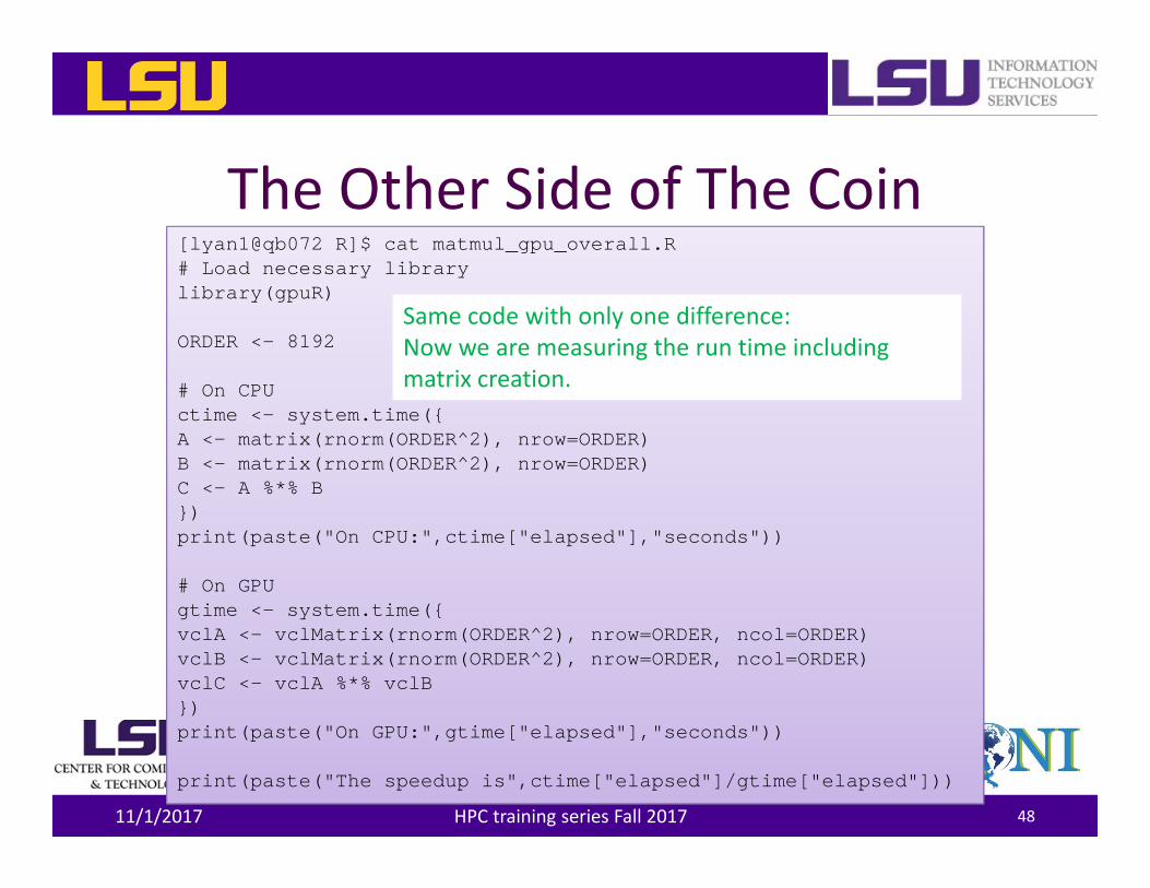
The Other Side of The Coin


[lyan1@qb072 R]$ cat matmul_gpu_overall.R# Load necessary librarylibrary(gpuR)

ORDER <- 8192

# On CPUctime <- system.time({A <- matrix(rnorm(ORDER^2), nrow=ORDER)B <- matrix(rnorm(ORDER^2), nrow=ORDER)C <- A %*% B})print(paste("On CPU:",ctime["elapsed"],"seconds"))

# On GPUgtime <- system.time({vclA <- vclMatrix(rnorm(ORDER^2), nrow=ORDER, ncol=ORDER)vclB <- vclMatrix(rnorm(ORDER^2), nrow=ORDER, ncol=ORDER)vclC <- vclA %*% vclB})print(paste("On GPU:",gtime["elapsed"],"seconds"))

print(paste("The speedup is",ctime["elapsed"]/gtime["elapsed"]))

Same code with only one difference:Now we are measuring the run time including matrix creation.

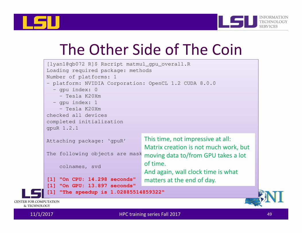
The Other Side of The Coin


[lyan1@qb072 R]$ Rscript matmul_gpu_overall.RLoading required package: methodsNumber of platforms: 1- platform: NVIDIA Corporation: OpenCL 1.2 CUDA 8.0.0



checked all devicescompleted initializationgpuR 1.2.1

Attaching package: ‘gpuR’

The following objects are masked from ‘package:base’:

colnames, svd

[1] "On CPU: 14.298 seconds"[1] "On GPU: 13.897 seconds"[1] "The speedup is 1.02885514859322"

This time, not impressive at all:Matrix creation is not much work, but moving data to/from GPU takes a lot of time. And again, wall clock time is what matters at the end of day.

Deep Learning in R• Since 2012, Deep Neural Network (DNN) has gained great

popularity in applications such as – Image and pattern recognition– Natural language processing

• There are a few R packages that support DNN– MXNet (multiple nodes with GPU support)– H2o (multiple nodes)– Darch– Deepnet– Rpud


References

• ParallelR (www.parallelr.com)– Code: https://github.com/PatricZhao/ParallelR

• R Documentation for packages mentioned in this tutorial


Thank you!


parallel computing with r - louisiana state university€¦ · · 2017-11-01parallel computing...

Documents