Parameter estimation in a reservoir engineering application

A. M. HaneaInstitute of Applied MathematicsDelft University of Technology, The Netherlands

M. GheorgheiBMG / iMTAErasmus University Rotterdam, The Netherlands

ABSTRACT: Reservoir simulation models are used both in the development of new fields, and in developedfields where production forecasts are needed for investment decisions. When simulating a reservoir one mustaccount for the physical and chemical processes taking place in the subsurface. Rock and fluid properties arecrucial when describing the flow in porous media. In this paper the authors are concerned with estimating thepermeability field of a reservoir. The problem of estimating model parameters such as permeability is oftenreferred to as a history matching problem in reservoir engineering. Currently one of the most widely usedmethodologies which address the history matching problem is the Ensemble Kalman filter (EnKF) (Evensenet al. 2007, Aanonsen et al. 2009). EnKF is a Monte-Carlo implementation of the Bayesian update problem.Nevertheless, the EnKF methodology has certain limitations. For this reason a new approach based on graphicalmodels is proposed and studied. In particular, the graphical model chosen for this purpose is a dynamic non-parametric Bayesian network (NPBN) (Hanea 2009, Gheorghe 2010). The NPBN based approach is comparedwith the EnKF method. A two phase, 2D flow model was implemented for a synthetic reservoir simulationexercise and the results of both methods for the history matching process of estimating the permeability fieldare illustrated and compared.

1 INTRODUCTION

The objective of reservoir engineering is to opti-mise hydrocarbon recovery. Oil and gas are generallyfound in sandstones or limestones. There are severalstages of the oil recovery process. In a primary recov-ery stage, reservoir drive comes from a number of nat-ural mechanisms. Primary oil recovery is the processof pumping out the oil that flows naturally to the bot-tom of the well due to gravity and the pressure of thereservoir. Primary recovery ends when the pressurebecomes too low. After that, one of the most com-mon and efficient secondary recovery processes is theinjection of water into an oil well, in order to forceout some of the remaining thicker crude oil. As thewater is forced into the reservoir, it spreads out fromthe injection well and pushes some of the remainingoil towards the producing wells 1. The properties ofthe rock, e.g. porosity and permeability, are therefore

1In the secondary recovery process the water can be replacedby gas. Steam, carbon dioxide, and other substances can be in-jected into an oil-producing unit in order to maintain reservoirpressure. This is known as tertiary recovery.

important for oil extraction since they influence theability of fluids to flow through the reservoir.

In this paper the authors are concerned with esti-mating the permeability field of a reservoir. The prob-lem of estimating model parameters such as perme-ability is often referred to as a history matching prob-lem in reservoir engineering.

To characterise the fluid flow into the reservoir weuse a two phase (oil-water), 2D flow model which canbe represented as a system of coupled nonlinear par-tial differential equations that cannot be solved ana-lytically. Consequently, we build a state-space modelfor the reservoir.

2 DYNAMIC NON - PARAMETRIC BAYESIANNETWORKS & KALMAN FILTER METHODS– DESCRIPTION & CONNECTION

In a state-space model, an underlying (hidden) state ofthe world that generates observations is assumed. Thishidden state is represented by a vector of variablesthat we cannot measure, but whose state we wouldlike to estimate. This hidden state vector evolves in

time. The goal of many applications is to infer thehidden state given the observations up to the currenttime.

Let Xt represent the hidden state at time t, andy1, .., yt the observations up to time t. The goal is tocompute P (Xt|y1, ..yt), called the belief state. We canupdate the belief state recursively using Bayes’ rule,and obtain a probability distribution over the hiddenstate.

A state-space model starts with a prior, P (X1), astate-transition function, P (Xt|Xt−1), and an obser-vation function, P (Yt|Xt)

2. We assume that the modelis first-order Markov, i.e., P (Xt|X1, ..,Xt−1) =P (Xt|Xt−1). Similarly, we can assume that the ob-servations are conditionally independent given themodel, i.e. P (Yt|Yt−1,Xt) = P (Yt|Xt). There aremany ways of representing state-space models, oneof the most common being the Kalman Filter (KF)model. KF assumes that Xt is a vector of continuousrandom variables, and that X1, ..,XT and Y1, .., YT arejoint normally distributed. The KF model was intro-duced by R. E. Kalman in 1960 (Kalman 1960). Theauthor proposes a recursive procedure for inferenceabout Xt:

Xt = GtXt−1 + wt;

Yt = FtXt + vt. (1)

The random variables wt and vt represent the pro-cess and measurement noise, respectively. They areassumed to be independent, white, and normally dis-tributed. In practice, the process noise covariance andmeasurement noise covariance matrices can changewith each time step or measurement, however herethey are assumed constant. Gt is a matrix that relatesthe state at the previous time step to the current step;Ft in the second equation of (1) relates the state to themeasurements. The KF model assumes that the sys-tem is joint normal. This means the belief state mustbe unimodal, which is inappropriate for many prob-lems, especially those involving discrete variables.The KF will recursively calculate the state vector Xt

along with its covariance matrix, conditioned on theavailable measurements up to time t, under the crite-rion that the estimated error covariance is minimum.Conditioning on the measurements is referred to asthe assimilation step of the procedure. The KF methodbecomes computationally expensive for large scalesystems and it is not suitable for non linear systems.There are several algorithms developed in order toovercome these limitations. An example of such algo-rithm is the ensemble Kalman filter (EnKF) (Evensen1994). EnKF represents the distribution of the sys-tem state using a collection of state vectors, called anensemble, and replaces the covariance matrix by the

2We can also consider input variables Ut. Then, the condi-tional probabilities become P (Xt|Xt−1,Ut) and P (Yt|Xt,Ut).In this paper Ut will not be considered.

sample covariance computed from the ensemble. Ad-vancing the probability distribution function in timeis achieved by simply advancing each member of theensemble. The main advantage of the EnKF is thatit approximates the covariance matrix from a finitenumber of ensemble members, thus becoming suit-able for large non linear problems. Nevertheless, veryoften the number of variables to be estimated is muchlarger than the number of ensemble members. Thereare typically millions of state variables and less thana hundred ensemble members (e.g. Li et al. (2003)).In these situations the ensemble covariance is rankdeficient, hence it contains large terms for pairs ofpoints that are spatially distant. These are called spu-rious correlations, and since they are not physicallyaccurate, there are algorithms that try to correct them(e.g. Anderson (2007),Hamill et al. (2001)). Unfortu-nately these algorithms introduce other inconsisten-cies in the system. Moreover, EnKF relays on the nor-mality assumption although it is often used in practicefor nonlinear problems, where this assumption maynot be satisfied.

Because of these limitations we introduce a moregeneral model, namely a dynamic Bayesian network(Dean and Kanazawa 1989, Dean and Wellman 1991).Dynamic Bayesian networks provide a much moreexpressive language for representing state-space mod-els. They can be interpreted as instances of a staticBayesian networks (BNs) (Pearl 1988) connected indiscrete slices of time3.

At this point, a brief description of static BNs isappropriate. A static BN is a directed acyclic graph(DAG) whose nodes represent univariate random vari-ables, which can be discrete or continuous, and thearcs represent direct influences. The BN stipulatesthat each variable is conditionally independent of allpredecessors in an (non-unique) ordering of the vari-ables, given its direct predecessors. The direct pre-decessors of a node i, corresponding to variable Xi

are called parents and the set of all i’s parents is de-noted Pa(i), or Pa(Xi). Since uncertainty distribu-tions need not conform to any parametric form, algo-rithms for specifying, sampling and analysing themshould be non-parametric. Therefore we shall usenon parametric Bayesian networks (NPBNs) (Hanea2008). NPBNs associate nodes with random vari-ables for which no marginal distribution assumptionis made, and arcs with conditional copulae (Joe 1997,Nelsen 1999). These conditional copulae, togetherwith the one-dimensional marginal distributions andthe conditional independence statements implied bythe graph uniquely determine the joint distribution,and every such specification is consistent (Hanea et al.2006). The marginal distributions can be obtainedfrom data or experts (Cooke 1991). Even thoughthe empirical marginal distributions are used in mostcases, parametric forms can be also fitted. The (condi-

3We only consider discrete-time stochastic processes.

Figure 1: The KF model as a dynamic BN

tional) copulae used in this method are parametrisedby (conditional) rank correlations that can be calcu-lated from data or elicited from experts (Morales,Kurowicka, & Roelen 2007). The name NPBN issomewhat inappropriate but it is used to stress the factthat the joint distribution is specified via marginal dis-tributions, upon which no restrictions are placed, andthe dependence structure given in terms of a non para-metric measure of dependence.

A dynamic NPBN is a way to extend a static NPBNto model probability distributions of collections ofrandom variables, Z1,Z2, ..,ZT . The variables canbe partitioned in Zt = (Xt, Yt) to represent the hid-den and output variables of a state-space model. Adynamic NPBN is defined to be a pair, (B1,B→),where B1 is a NPBN which defines the prior P (Z1),and B→ is a two-slice temporal NPBN which definesP (Zt|Zt−1) as follows:

P (Zt|Zt−1) =∏

i

P (Zit |Pa(Zi

t)), (2)

where Zit is the ith node at time t, which could be a

component of Xt, or of Yt.The parents Pa(Zi

t) can be either in the same timeslice or in the previous time slice4.The arcs betweenslices are from left to right, reflecting the flow of time.

The difference between a dynamic NPBN and aKF model is that the latter requires joint normality,whereas a dynamic NPBN allows arbitrary marginaldistributions. In addition, a dynamic NPBN allowsfor a much more general graph structure. Figure 1presents a general KF model as a dynamic BN.

3 CASE STUDY

We construct a synthetic example by simulatinga five-spot injection-production strategy. In otherwords, the reservoir has an injector in the middle ofthe field (where water is injected) and 4 producers,one in each corner (where oil is pumped out from).The true permeability field is randomly chosen froman ensemble of possible models (see Figure 2) andthe synthetic production data is generated using thistrue model. Synthetic measurements are obtained byadding normally distributed errors to the productiondata.

4We assume the model is first-order Markov, for a fair com-parison with the ENKF method.

True permeability field

5 10 15 20

2

4

6

8

10

12

14

16

18

20−31

−30.5

−30

−29.5

−29

−28.5

Figure 2: The true permeability field.

3.1 Experimental setup

The reservoir model considered here is a 2D squarewith a uniform Cartesian grid consisting of 21 gridcells in each direction. The reservoir is considered aclosed space where liquid gets in and out only throughthe drilled wells. Therefore, the drilled wells becomethe reservoir’s boundaries. A well model is availablefor the injection and extraction of fluids through thedrilled wells. The flow is specified at the wells bybottom hole pressure (bhp) and fluid flow rates (q).The well model imposes that either the bottom holepressure or the fluid flow rates must be prescribed.We consider the case where the injection well is con-strained by prescribed flow rates and production wellsare constrained by bottom hole pressure. The twophase flow model is combined with the well modeland implemented in a simple in-house simulator.

The state vector contains pressures (p) correspond-ing to each grid cell. Since we want to perform a pa-rameter estimation, the state vector is augmented withthe parameter of interest, i.e. the natural logarithm ofthe permeability5 (log(k)). Given the well model con-straints, we measure bottom hole pressure at the in-jector and total flow rates at the producers. The finalform of the vector Zt is:

Zt =

logk(t)p(t)

bhp(t)q(t)

The reservoir is initialized with pressure equal to 3 ·107[Pa] in every grid cell. We perform simulations for420 days, considering measurements every 60 days.

For the NPBN based approach we build a DAGon the variables defined in the state vector, hence theDAG should contain 1328 nodes. Given the incipientstage of modelling a petroleum engineering problemwith a NPBN, a simplification of the model is in or-der. Based on expert’s opinions we decided to excludethe variables representing saturations and how to setthe arc directionality amongst remaining variables. A

5We consider the log(k) instead of k because the values of thepermeability are of order 10−13[m2].

Figure 3: The DAG of the NPBN.

schematic representation of a potential BN is shownin Figure 3.

3.2 Results & comparisons

We will first estimate the permeabilities in a reducednumber of grid cells. The initial goal of this studywas to estimate the entire permeability field with bothmethods and compare results. Unfortunately, at thisstage of the research, the NPBN approach cannot han-dle more than 500 variables, so we shall restrict ouranalysis to parts of the grid, rather than the entirereservoir.

We arbitrarily choose 4 different locations. Wemeasure bottom hole pressure (bhp) at the injectorwell and the total flow rates (q) denoted now by to-tal rate i, i = 1, ..,4, at each producer. Any loca-tion that is not a well has its corresponding pressureand permeability. We denote them by p j, and k j,j = 6, ..,9, respectively. Therefore, we are interestedin the joint distribution of 13 variables. We run thesimulator for the first 60 days, and obtain their jointdistribution (in form of a data set). We can now rep-resent the joint distribution using a static NPBN. Us-ing a saturated NPBN6 translates into representing allpossible dependencies present in the data set, includ-ing the noisy ones. Moreover, the visual advantage ofthe graphical model vanishes since a saturated graphis dense and un-intuitive. Another choice is to learna validated NPBN from data. A learning algorithm isintroduced in Hanea et al. (2010). The only assump-tion of the algorithm is that of a joint normal copula.This means that we model the data as if it were trans-formed from a joint normal distribution. The marginaldistributions are taken directly from data and the em-pirical rank correlation matrix is calculated. The algo-rithm assigns arcs between strongly correlated vari-ables. Missing arcs will correspond to (conditional)independent statements. A joint distribution that ap-proximates the distribution given by the simulator is

6In a saturated NPBN all nodes are connected.

Figure 4: The learned NPBN after 60 days.

therefore obtained. For details we refer to Hanea et al.(2010). The learning procedure involves validation.First, we validate that the joint normal copula ade-quately represents the multivariate data. If this is thecase we then learn a model and validate that it is anadequate model of the saturated graph.

After 60 days, the normal copula assumption is val-idated, hence we learn the NPBN presented in Fig-ure 4. The NPBN model is build using the softwareUninet (Morales-Napoles et al. 2007). Nodes of anNPBN can be visualised as ellipses or histograms.The mean and standard deviation of each variable areshown on the graph.

The static NPBN can now be used to performthe conditionalization/assimilation step. Given the ob-served values of measurements at the wells, we cancalculate the joint conditional distribution of the othervariables7. It is worth noting that the observable vari-ables are not normally distributed. Nevertheless, nor-mally distributed noise is added when generatingmeasurements for a fair comparison with the EnKFmethod. After conditioning, we stipulate the condi-tional distribution by sampling it. Further, we intro-duce the updated distribution in the simulator, and werun it for another 60 days. In this way we obtain thedistribution of the variables after 120 days (with 1 as-similation step after 60 days). The new joint distribu-tion will be modelled with another static NPBN. The2 NPBNs connected through the simulator are basi-cally a dynamic NPBN with changed structure andparameters over time, and with functional temporalrelationships. We repeat the above steps for a periodof 420 days. Every time step we validate the nor-mal copula and the model. We thus build a dynamicNPBN for 7 discrete times.

The results of estimating the permeabilities for thechosen locations using a saturated NPBN, a learnedNPBN, and the EnKF method are further presented.To measure the quality of the estimation we compareit with the truth. A measure of discrepancy is the root

7The normal copula assumption facilitates analytical condi-tioning (Hanea et al. 2006).

0 200 400 6000

0.5

1

1.5

2

2.5

3

Time [days]

RMSE for Location 6

EnKFThe Saturated NPBNThe Learned NPBN

0 200 400 6000

0.5

1

1.5

Time [days]

RMSE for Location 7

EnKFThe Saturated NPBNThe Learned NPBN

0 200 400 6000

0.5

1

1.5

Time [days]

RMSE for Location 8

EnKFThe Saturated NPBNThe Learned NPBN

0 200 400 6000

0.5

1

1.5

2

2.5

Time [days]

RMSE for Location 9

EnKFThe Saturated NPBNThe Learned NPBN

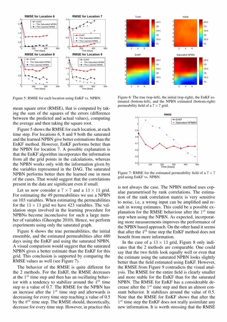
Figure 5: RMSE for each location using EnKF vs. NPBN.

mean square error (RMSE), that is computed by tak-ing the sum of the squares of the errors (differencebetween the predicted and actual values), computingthe average and then taking the square root.

Figure 5 shows the RMSE for each location, at eachtime step. For locations 6, 8 and 9 both the saturatedand the learned NPBN give better estimations than theEnKF method. However, EnKF performs better thanthe NPBN for location 7. A possible explanation isthat the EnKF algorithm incorporates the informationfrom all the grid points in the calculations, whereasthe NPBN works only with the information given bythe variables represented in the DAG. The saturatedNPBN performs better then the learned one in mostof the cases. That would suggest that the correlationspresent in the data are significant even if small.

Let us now consider a 7 × 7 and a 13 × 13 grid.For estimating the 49 permeabilities we use a NPBNon 103 variables. When estimating the permeabilitiesfor the 13× 13 grid we have 423 variables. The val-idation steps involved in the learning procedure forNPBNs become inconclusive for such a large num-ber of variables (Gheorghe 2010). Hence, we performexperiments using only the saturated graph.

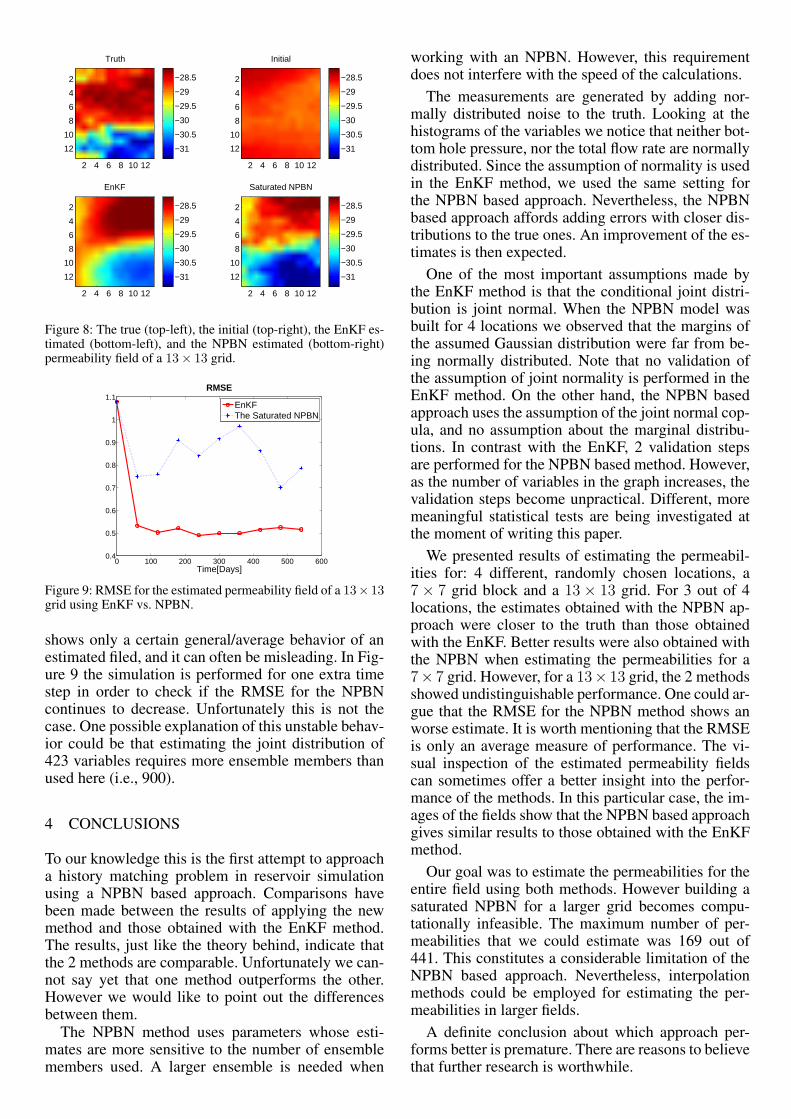
Figure 6 shows the true permeabilities, the initialensemble, and the estimated permeabilities after 480days using the EnKF and using the saturated NPBN.A visual comparison would suggest that the saturatedNPBN gives a better estimate than the EnKF for thisgrid. This conclusion is supported by comparing theRMSE values as well (see Figure 7).

The behavior of the RMSE is quite different forthe 2 methods. For the EnKF, the RMSE decreasesat the 1st time step and then has an oscillating behav-ior with a tendency to stabilize around the 4th timestep to a value of 0.7. The RMSE for the NPBN hasan increase after the 1st time step and afterwards isdecreasing for every time step reaching a value of 0.5by the 8th time step. The RMSE should, theoretically,decrease for every time step. However, in practice this

Truth

2 4 6

1

2

3

4

5

6

7 −31

−30.5

−30

−29.5

−29

−28.5

Initial

2 4 6

1

2

3

4

5

6

7 −31

−30.5

−30

−29.5

−29

−28.5

EnKF

2 4 6

1

2

3

4

5

6

7 −31

−30.5

−30

−29.5

−29

−28.5

Saturated NPBN

2 4 6

1

2

3

4

5

6

7 −31

−30.5

−30

−29.5

−29

−28.5

Figure 6: The true (top-left), the initial (top-right), the EnKF es-timated (bottom-left), and the NPBN estimated (bottom-right)permeability field of a 7× 7 grid.

0 100 200 300 400 5000.4

0.5

0.6

0.7

0.8

0.9

1

1.1

Time [Days]

RMSE

EnKFSaturated NPBBN

Figure 7: RMSE for the estimated permeability field of a 7× 7grid using EnKF vs. NPBN.

is not always the case. The NPBN method uses cop-ulae parametrised by rank correlations. The estima-tion of the rank correlation matrix is very sensitiveto noise, i.e, a wrong input can be amplified and re-sult in wrong estimates. This could be a possible ex-planation for the RMSE behaviour after the 1st timestep when using the NPBN. As expected, incorporat-ing more measurements improves the performance ofthe NPBN based approach. On the other hand it seemsthat after the 4th time step the EnKF method does notbenefit from more information.

In the case of a 13× 13 grid, Figure 8 only indi-cates that the 2 methods are comparable. One couldsay that the two fields look equally well or even thatthe estimate using the saturated NPBN looks slightlybetter than the field estimated using EnKF. However,the RMSE from Figure 9 contradicts the visual anal-ysis. The RMSE for the entire field is clearly smallerand more stable for the EnKF than for the saturatedNPBN. The RMSE for EnKF has a considerable de-crease after the 1st time step and then an almost con-stant behavior. It stabilizes around the value of 0.5.Note that the RMSE for EnKF shows that after the1st time step the EnKF does not really assimilate anynew information. It is worth stressing that the RMSE

Truth

2 4 6 8 10 12

2

4

6

8

10

12

Initial

2 4 6 8 10 12

2

4

6

8

10

12

EnKF

2 4 6 8 10 12

2

4

6

8

10

12

−31

−30.5

−30

−29.5

−29

−28.5

−31

−30.5

−30

−29.5

−29

−28.5

−31

−30.5

−30

−29.5

−29

−28.5

Saturated NPBN

2 4 6 8 10 12

2

4

6

8

10

12 −31

−30.5

−30

−29.5

−29

−28.5

Figure 8: The true (top-left), the initial (top-right), the EnKF es-timated (bottom-left), and the NPBN estimated (bottom-right)permeability field of a 13× 13 grid.

0 100 200 300 400 500 6000.4

0.5

0.6

0.7

0.8

0.9

1

1.1

Time[Days]

RMSE

EnKFThe Saturated NPBN

Figure 9: RMSE for the estimated permeability field of a 13× 13grid using EnKF vs. NPBN.

shows only a certain general/average behavior of anestimated filed, and it can often be misleading. In Fig-ure 9 the simulation is performed for one extra timestep in order to check if the RMSE for the NPBNcontinues to decrease. Unfortunately this is not thecase. One possible explanation of this unstable behav-ior could be that estimating the joint distribution of423 variables requires more ensemble members thanused here (i.e., 900).

4 CONCLUSIONS

To our knowledge this is the first attempt to approacha history matching problem in reservoir simulationusing a NPBN based approach. Comparisons havebeen made between the results of applying the newmethod and those obtained with the EnKF method.The results, just like the theory behind, indicate thatthe 2 methods are comparable. Unfortunately we can-not say yet that one method outperforms the other.However we would like to point out the differencesbetween them.

The NPBN method uses parameters whose esti-mates are more sensitive to the number of ensemblemembers used. A larger ensemble is needed when

working with an NPBN. However, this requirementdoes not interfere with the speed of the calculations.

The measurements are generated by adding nor-mally distributed noise to the truth. Looking at thehistograms of the variables we notice that neither bot-tom hole pressure, nor the total flow rate are normallydistributed. Since the assumption of normality is usedin the EnKF method, we used the same setting forthe NPBN based approach. Nevertheless, the NPBNbased approach affords adding errors with closer dis-tributions to the true ones. An improvement of the es-timates is then expected.

One of the most important assumptions made bythe EnKF method is that the conditional joint distri-bution is joint normal. When the NPBN model wasbuilt for 4 locations we observed that the margins ofthe assumed Gaussian distribution were far from be-ing normally distributed. Note that no validation ofthe assumption of joint normality is performed in theEnKF method. On the other hand, the NPBN basedapproach uses the assumption of the joint normal cop-ula, and no assumption about the marginal distribu-tions. In contrast with the EnKF, 2 validation stepsare performed for the NPBN based method. However,as the number of variables in the graph increases, thevalidation steps become unpractical. Different, moremeaningful statistical tests are being investigated atthe moment of writing this paper.

We presented results of estimating the permeabil-ities for: 4 different, randomly chosen locations, a7× 7 grid block and a 13× 13 grid. For 3 out of 4locations, the estimates obtained with the NPBN ap-proach were closer to the truth than those obtainedwith the EnKF. Better results were also obtained withthe NPBN when estimating the permeabilities for a7× 7 grid. However, for a 13× 13 grid, the 2 methodsshowed undistinguishable performance. One could ar-gue that the RMSE for the NPBN method shows anworse estimate. It is worth mentioning that the RMSEis only an average measure of performance. The vi-sual inspection of the estimated permeability fieldscan sometimes offer a better insight into the perfor-mance of the methods. In this particular case, the im-ages of the fields show that the NPBN based approachgives similar results to those obtained with the EnKFmethod.

Our goal was to estimate the permeabilities for theentire field using both methods. However building asaturated NPBN for a larger grid becomes compu-tationally infeasible. The maximum number of per-meabilities that we could estimate was 169 out of441. This constitutes a considerable limitation of theNPBN based approach. Nevertheless, interpolationmethods could be employed for estimating the per-meabilities in larger fields.

A definite conclusion about which approach per-forms better is premature. There are reasons to believethat further research is worthwhile.

REFERENCES

Aanonsen, S., G. Naedval, D. Oliver, A. Reynolds, & B. Valles(2009). The Ensemble Kalman Filter in Reservoir Engineer-ing. SPE Journal.

Anderson, J. (2007). Exploring the need for localization in en-semble data assimilation using a hierarchical ensemble filter.Physica D: Nonlinear Phenomena, 99111.

Cooke, R. (1991). Experts in Uncertainty : Opinion and Subjec-tive Probability in Science. Environmental Ethics and Sci-ence Policy Series. Oxford University Press.

Dean, T. & K. Kanazawa (1989). A model for reasoning aboutpersistence and causation. Artificial Intelligence 93(1-2),127.

Dean, T. & M. Wellman (1991). Planning and control. MorganKaufmann.

Evensen, G. (1994). Sequential data assimilation with nonlinearquasi-geostrophic model using Monte Carlo methods to fore-cast error statistics. Journal of Geophysical Research 99(C6),1014310162.

Evensen, G., J. Hove, H. Meisingset, E. Reiso, K. Seim, & O. Es-pelid (2007). Using the EnKF for assisted history matchingof a North Sea reservoir model. SPE Reservoir SimulationSymposium Huston(Texas), USA.

Gheorghe, M. (2010). Non parametric Bayesian belief nets ver-sus ensemble Kalman Filter in reservoir simulation. MScThesis, Delft University of Technology.

Hamill, T., J. Whitaker, & C. Snyder (2001). Distance-dependentfiltering of background error covariance estimates in anensemble Kalman filter. Monthly Weather Review 129,27762790.

Hanea, A. (2008). Algorithms for Non-parametric Bayesian be-lief nets. Ph. D. thesis, TU Delft, Delft, the Netherlands.

Hanea, A. (2009). Tackling a Reservoir Engineering Problemwith a NPBN Approach. Lecture notes, Summer School onData Assimilation: Section 3.

Hanea, A., D. Kurowicka, & R. Cooke (2006). Hybrid Methodfor Quantifying and Analyzing Bayesian Belief Nets. Qualityand Reliability Engineering International 22(6), 613–729.

Hanea, A., D. Kurowicka, R. Cooke, & D. Ababei (2010). Min-ing and visualising ordinal data with non-parametric con-tinuous BBNs. Computational Statistics and Data Analy-sis 54(3), 668–687.

Joe, H. (1997). Multivariate Models and Dependence Concepts.London: Chapman & Hall.

Kalman, R. (1960). A new approach to linear filtering and pre-diction problems. Journal of Basic Engineering, 3545.

Li, R., A. C. Reynolds, & D. Olivier (2003). History matchingof three phase flow production data. SPE Journal 8(4), 328–340.

Morales, O., D. Kurowicka, & A. Roelen (2007). Eliciting con-ditional and unconditional rank correlations from conditionalprobabilities. Reliability Engineering and System Safety. doi:10.1016/j.ress.2007.03.020.

Morales-Napoles, O., D. Kurowicka, R. Cooke, & D. Ababei(2007). Continuous-discrete distribution free Bayesian beliefnets in aviation safety with UNINET. Technical Report TUDelft.

Nelsen, R. (1999). An Introduction to Copulas. Lecture Notes inStatistics. New York: Springer - Verlag.

Pearl, J. (1988). Probabilistic Reasoning in Intelligent Systems:Networks of Plausible Inference. San Mateo: Morgan Kauf-man Publishers.