parameterizing the trifocal tensor - computer …€¦ · parameterizing the trifocal tensor may...

$: Parameterizing the Trifocal Tensor - Computer …€¦ · Parameterizing the Trifocal Tensor May 11, 2017 Based on: Klas Nordberg. \A Minimal Parameterization of the Trifocal Tensor"$
Parameterizing the Trifocal Tensor

May 11, 2017

Based on:

Klas Nordberg. “A Minimal Parameterization of the Trifocal Tensor”. InComputer society conference on computer vision and pattern recognition (CVPR).

2009

Silver (Joni) De Guzman and Anthony Thomas

May 11, 2017 1 / 44

What is the Trifocal Tensor and Why Should we Care?

Encodes the geometric relationship between three corresponding views.

Analogous to the fundamental matrix of two-view geometry, but trifocaltensor extends to three-views.

Can be determined only from feature correspondences between three images.

Applications:I Accurate 3D scene reconstructionI RoboticsI Virtual and augmented reality

May 11, 2017 2 / 44

Why Use Three Views Instead of Two?

The geometry on an image sequence can be more accurately and robustlydetermined from image triplets than image pairs.

More views means more accuracy for reconstruction.

May 11, 2017 3 / 44

3D Reconstruction

Building Rome (Actually Dubrovnik) in a Day

University of Washington Grail LabMay 11, 2017 4 / 44

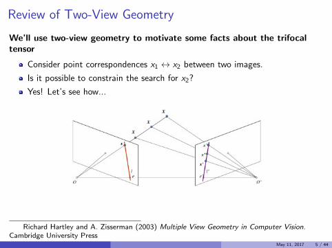
https://www.youtube.com/watch?v=sQegEro5Bfo&index=4&list=PLDFDB5B8C80DB3AD6

Review of Two-View Geometry

We’ll use two-view geometry to motivate some facts about the trifocaltensor

Consider point correspondences x1 ↔ x2 between two images.

Is it possible to constrain the search for x2?

Yes! Let’s see how...

Richard Hartley and A. Zisserman (2003) Multiple View Geometry in Computer Vision.Cambridge University Press

May 11, 2017 5 / 44

The Fundamental Matrix

The Fundamental MatrixThe fundamental matrix F encodes the geometric relationship between two views.

F maps points in view one to epipolar lines in view two: l ′ = Fx .

For any corresponding x ↔ x ′: xFx ′ = 0.

We can determine F without knowing anything about the underlying cameras!

May 11, 2017 6 / 44

The Fundamental Matrix

An Important Note:

The fundamental matrix is invariant to projective transformations (denoted H) ofthe 3D scene.

Why?

C1X = (C1H)(H−1X) and C2X = (C2H)(H−1X)

If x1 and x2 are matched under C1 and C2 then they’re still matched underthe transformation.

Implication: two projection matrices uniquely determine the fundamentalmatrix, but the converse is not true!


May 11, 2017 7 / 44

Introducing the Trifocal Tensor

What happens when we introduce a third view?

Meet the Trifocal Tensor

May 11, 2017 8 / 44

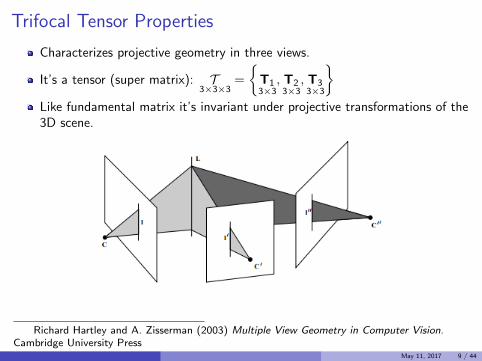
Trifocal Tensor Properties

Characterizes projective geometry in three views.

It’s a tensor (super matrix): T3×3×3

=

{T13×3

, T23×3

, T33×3

}Like fundamental matrix it’s invariant under projective transformations of the3D scene.


May 11, 2017 9 / 44

Structure of the Tensor

Structure of the TensorThe Trifocal Tensor can be computed from the camera projection matrices:C1 = (I | 0) ,C2 = (A | a4) ,C3 = (B | b4)

C2 =

a11 a12 a13 a14a21 a22 a23 a24a31 a32 a33 a34

C3 =

b11 b12 b13 b14b21 b22 b23 b24b31 b32 b33 b34

⇒ Ti = aibT4 − a4b

Ti

This works in reverse too: given T we can recover C1,C2,C3 and their epipoles

May 11, 2017 10 / 44

Degrees of Freedom

Any tensor computed from three camera matrices is said to be “consistent”(geometrically valid).

Ci3×4

has 11 dof ×3 cameras = 33 degrees of freedom. But...

Invariant under projective transformations H4×4

so: 33− 15 = 18 dof.

Any geometrically valid T satisfies 27− 18− 1 = 8 internal constraints.I Analogous to the det(F) = 0 constraint on the fundamental matrix.I But much more complicated so we won’t talk about them here...

May 11, 2017 11 / 44

Comparison of Fundamental Matrix and Trifocal Tensor

Fundamental Matrix

2 views

3x3 matrix with 9 elements

7 degrees of freedom

1 internal constraint: det(F) = 0

minimum 7 point correspondences

depends solely on featurecorrespondences

Trifocal Tensor

3 views

3x3x3 tensor with 27 elements

18 degrees of freedom

8 internal constraints

minimum 6 point correspondences

depends solely on featurecorrespondences

May 11, 2017 12 / 44

The Trilinear Relations I

Just like F, the trifocal tensor encodes relationships between points and linesin the three views.

Point-Point-Point

/

/ /

x

x / /

X

x /

C

C

C

[x′]x

(∑i

x iTi

)[x′′]x = 0

May 11, 2017 13 / 44

The Trilinear Relations II

Point-Line-Line

/

X

l

C

/

L

/ /

C

Cx

/x

l//

x//

l′T

(∑i

x iTi

)l′′ = 0

We get lots more: point-line-point, point-point-line, etc...


May 11, 2017 14 / 44

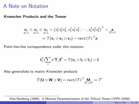
A Note on Notation

Kronecker Products and the Tensor

x13×1⊗ x2

3×1⊗ x3

3×1=(x11 x

12 x

13 , x

11 x

12 x

23 , · · · , x31 x32 x33

)T= a

27×1

⇒ T (x1 ⊗ x2 ⊗ x3) = vect(T )Ta

Point-line-line correspondence under this notation:

lT2 (∑i

x iTi )l3 = T (x1 ⊗ l2 ⊗ l3) = 0

Also generalizes to matrix Kronecker products

T (U⊗W ⊗ V) = vect(T )T M27×27

⇒ T ′

Klas Nordberg (2009). A Minimal Parameterization of the Trifocal Tensor CVPR (2009).May 11, 2017 15 / 44

Estimating the Tensor

The heavily condensed version:

1 Detect feature correspondences and apply MSAC outlier-rejection (requires 6point correspondences).

2 Apply a linear algorithm (DLT) to obtain an initial estimate T0I T0 needs to satisfy the eight internal constraints.I Apply another round of estimation minimizing algebraic error.I Or maybe something else...

3 Apply the Levenberg-Marquardt algorithm to obtain the “gold-standard”estimate minimizing geometric error (easier said than done).


May 11, 2017 16 / 44


How should we parameterize the tensor?

May 11, 2017 17 / 44


Klas Nordberg. “A Minimal Parameterization of the Trifocal Tensor”. InComputer society conference on computer vision and pattern recognition (CVPR).

2009

Proposition

The trifocal tensor may be parameterized by three 3× 3 orthogonal matrices anda homogeneous 10-vector.

The proof of this follows on the next many slides. In the words of the author:“Here we go!”


Some Terminology

Skew-Symmetric Matrices and Cross-Products:

[a]x =

0 −a3 a2a3 0 −a1−a2 a1 0

Note: [a]x b = −bT [a]x = a× b

A couple other useful properties: [a]x a = 0 and bT [a]x b = 0

Remember the Kronecker Product:

T(

U3×3⊗ W

3×3⊗ V

3×3

)= vect(T )T M

27×27⇒ T ′


Problem Setup

Let C1,C2,C3 be three generic camera matrices.I Ci = (Ri | ti )

We want the cameras to be canonical to deal with projective ambiguity

We’ll “rotate” the first camera so it aligns with the scene plane

SVD(C1) = L3×3

(S | 0)3×4

H4×4

⇒ C′1 = S−1LTC1H = (I | 0)

⇒ C′2 = C2H = (A | a4)

⇒ C′3 = C3H = (B | b4)


Problem Setup

Now we can use the “nice” form of T : Ti = aibT4 − a4b

Ti

Let T ′ be the “canonical” tensor and let T be the “raw” one

We want a way to go back and forth: T ′ ↔ TWe can show this relationship is well defined and described by the following:

T ′ = T (S−1LT ⊗ I⊗ I) = T (D⊗ I⊗ I)

Takeaway:

We can transform the scene such that the first camera is “canonical.” There existsa well defined relationship between T ′ and T and we can use T ′ from now on.


Another Proposition

Proposition

There exists three orthogonal matrices U,V,W which can be used to transformthe trifocal tensor such that exactly ten well defined elements are non-zero.



Consider the following transformation:

T̃ ′jki =∑m,p,q

T ′pqm Umi V j

pWkq

=∑m

umi(vTp Tmwq

)T̃ ′ = T ′ (U⊗ V ⊗W)

Intuition:

Elements of T̃ ′ are formed by multiplying triplets of columns from U,V,W onto“slices” of T ′

We’ll now show that for the correct choice of U,V,W something pretty coolhappens...


Parameterizing The Trifocal Tensor

Consider the following matrices whose columns are orthogonal:

U0 =

(A−1a4,

[A−1a4

]2xB−1b4,

[A−1a4

]xB−1b4

)(1)

V0 =(a4, [a4]x AB

−1b4, [a4]2x AB−1b4

)(2)

W0 =(b4, [b4]x BA

−1a4, [b4]2x BA−1a4

)(3)

Lemma:For a matrix M0 with orthogonal columns, the transformation

M = M0(MT0 M0)

−12 yields an orthogonal matrix.


Proof of the Proposition

First some preliminaries:

Define: r = AB−1b4, r′ = [a4]x r, s = BA−1a4, s

′ = [b4]x s.

Then: V0 = (a4, [a4]x r, [a4]x r′, [a4]x r

′) and W0 = (b4, [b4]x s, [b4]x s′)

The transformation M0 →M simply rescales the columns of M so it sufficesto prove the proposition using U0,V0,W0.



Remember the transformation: T̃ ′jki = T ′pqm Umi V j

pWkq ?

1 We want to show 17 elements of T̃ ′ are zero under this transformation.

2 The full proof is tedious so we’ll provide the necessary intuition.

3 Let’s look at how we can show some elements to be zero...


Proof of the PropositionFirst we’ll look at:

T̃ ′22i = T ′pqm UiV2pW

2q =

∑m,p,q

T ′pqm UiV2pW

2q = Uiv

T2 T′iw2 ∀i

Want to show:

V =

v1 v2 v3v11 v12 v13v21 v22 v23v31 v23 v33

W =

w1 w2 w3

w11 w12 w13

w21 w22 w23

u31 w23 w33

×Ti =

T11 T12 T13

T21 T22 T23

T31 T23 T33

⇒ T̃′i =

× × ×× 0 ×× × ×

Klas Nordberg (2009). A Minimal Parameterization of the Trifocal Tensor CVPR (2009).

May 11, 2017 27 / 44


To start note: ∑m,p,q

T ′pqm UiV2pW

2q = Uiv

T2 T′iw2 ∀i

If we can show vT2 T′iw2 = 0 then we can forget about Ui so:

T̃ ′22i = vT2 T′iw2

Now let’s plug in the definitions of Ti , vT2 , and w2:

T̃ ′22i = rT [a4]Tx

(aib

T4 − a4b

Ti

)[b4]x s

Then we can distribute as follows:

T̃ ′22i = rT [a4]Tx aibT4 [b4]x s− rT [a4]Tx a4b

Ti [b4]x s



Now let’s recall that a× a = 0 and note that we can take advantage of this here:

T̃ ′22i = rT [a4]Tx ai bT4 [b4]x s− rT [a4]Tx a4 bTi [b4]x s

Which gives us the desired result!

T̃ ′22i = rT · 0− 0 · s = 0



We can apply similar techniques to transform T into:

T̃′1 =

× 0 ×0 0 00 0 0

T̃′2 =

× 0 ×0 0 0× 0 0

T̃′3 =

× × ×× 0 0× 0 0

Note: this was the simplest case but all the other derivations use the same basictechnique...


Some Intuition

Where did the orthogonal matrices come from?

Meditating in the woods of Sweden?

“Medication”?

Careful exploitation of the internal structure of T and properties of the crossproduct?

The Orthogonal Matrices

U,V,W and Ti are all constructed using the camera matrices. It is theinteraction of the columns of the orthogonal matrices and the slices of T whichallow us to exploit properties of the cross product which cause certain elements tobecome zero.

May 11, 2017 31 / 44

Coming Full Circle

What Exactly Have We Shown?

The trifocal tensor can be transformed using three orthogonal matrices into asparse form with exactly ten non-zero elements

We’ve proved the proposition but so what?

We know how to parameterize this space!

The three orthogonal matrices may be parameterized using matrixexponentials ([ωw]x = log (W)) yielding nine parameters.

The ten non-zero elements may be parameterized as a homogeneous vectoryielding the remaining nine parameters.


Un-Canonicalizing the Transformations

We’ve found our minimal parameterization - But wait - there’s a catch...

The derivations above assumed canonical cameras. We need to undo the originalcanonicalization.

May 11, 2017 33 / 44


T̃ ′jki = T ′pqm Umi V j

pWkq = T ′(U⊗ V ⊗W)

recall: T ′ = T (D⊗ I⊗ I) so:

T̃ ′ = T (D⊗ I⊗ I)(U⊗ V ⊗W) = T (DU⊗ V ⊗W)

In general DU will not be orthogonal

So let’s take a QR decomposition: DU = QRI Q is orthogonal and R is upper-triangular

Now we have what we need:

T̃ ′ = T (Q⊗ V ⊗W)(R⊗ I⊗ I)

⇒ T̃ = T̃ ′(R−1 ⊗ I⊗ I) = T (Q⊗ V ⊗W)



What Have We Shown?The relationship between the sparse tensor and the original tensor without theassumption of canonical cameras is well defined.

This relationship is described by:

T = T̃ (QT ⊗ VT ⊗WT )


Are We Done?

Now we’re done!

Or are we...

May 11, 2017 36 / 44

Determining the Orthogonal Transformations

We’ve said nothing about how to determine U,V,W in practice.

Given noisy data we can’t expect to perfectly recover the sparse form

We instead wish to find the U,V,W which minimize the sum of squares ofthe zero valued elements.

Stated mathematically: we wish to solve the following minimization:

minU,V,W

||Pz [T (Q⊗ V ⊗W)] ||2

Where PZ is a projection operator mapping the zero valued elements of T̃ ′ toeuclidean space.


Determining the Orthogonal Transformations

This problem can be solved using standard nonlinear optimization techniques

Use the DLT algorithm to initialize T0. Extract the projection matrices toinitialize U,V,W. Apply LM to solve the problem above.

This gives a corrected estimate of T0 to which the “gold-standard” MLEestimate minimizing geometric error can be applied using the sameparameterization.

Bam! You’ve got yourself a trifocal tensor satisfying the eight internalconstraints


Some Concluding Points

This parameterization also allows us to enforce the internal constraints on alinear estimate

We can show (but won’t) that T0 is the best approximation to the “true”trifocal tensor satisfying the internal constraints.

But maybe the DLT is almost as good...

Does this really get us anywhere?


Experimental Evaluation

Experimental Set Up

Generate synthetic projection matrices and a 3D scene

Project the scene under each matrix and add some noise

Measure the distance between the “true” epipole e21 and its positionestimated from T .

Compare:1 T0: “Vanilla” DLT algorithm2 T1: “Sparse” algorithm without data normalization3 T2: “Sparse” algorithm with data normalization

Repeat 1000 times for varying number of image correspondences (N)


Experimental Evaluation

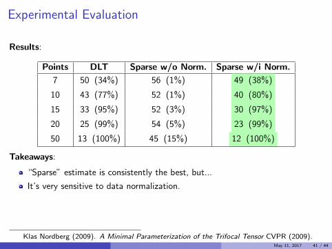
Results:

Points DLT Sparse w/o Norm. Sparse w/i Norm.

7 50 (34%) 56 (1%) 49 (38%)

10 43 (77%) 52 (1%) 40 (80%)

15 33 (95%) 52 (3%) 30 (97%)

20 25 (99%) 54 (5%) 23 (99%)

50 13 (100%) 45 (15%) 12 (100%)

Takeaways:

“Sparse” estimate is consistently the best, but...

It’s very sensitive to data normalization.


Now We’re Really Done

What Have We Shown?

Any Trifocal Tensor can be expressed using three rotation matrices and a10-vector.

This leads to a straightforward parameterization.

Which leads to better estimates than current “state-of-the-art” (from 2003).


3D Reconstruction Again

Byrod, Josephson and Astrom Fast Optimal Three View Triangulation. In ComputerVision-ACCV 2007.

May 11, 2017 43 / 44

Questions?

(1) Hedborg, Robinson and Felsberg. Robust Three View Triangulation Done Fast. In CVPR2014. (2) Nister. Reconstruction from Uncalibrated Sequences with a Hierarchy of TrifocalTensors. In ECCV00, volume 1, 2000.

May 11, 2017 44 / 44

parameterizing the trifocal tensor - computer …€¦ · parameterizing the trifocal tensor may...

Documents