part two: simulink getting started · steps in using simulink. though this tutorial covers the...

[ MATLAB ] [ Resources ]

Contents

l Introduction l Getting Started l Handling of Blocks and Lines l Annotations l Some Examples

Introduction

Simulink (Simulation and Link) is an extension of MATLAB by Mathworks. It works with MATLAB to offer modeling, simulating, and analyzing of dynamical systems under a graphical user interface (GUI) environment. The construction of a model is simplified with click-and-drag mouse operations. Simulink includes a comprehensive block library of toolboxes for both linear and nonlinear analyses. Models are hierarchical, which allow using both top-down and bottom-up approaches. As Simulink is an integral part of MATLAB, it is easy to switch back and forth during the analysis process and thus, the user may take full advantage of features offered in both environments. This tutorial presents some basic steps in using Simulink. Though this tutorial covers the general aspects of Simulink, the focus is on Control Systems as this has been written for my Control Systems students.

Getting Started

Starting SIMULINK

In MATLAB command window, enter: >> simulink and press ENTER to invoke Simulink.

A Simulink Library Browser window should appear as one shown below.

PART TWO: SIMULINK

NOTE: This tutorial is based on Simulink Version 3.0.1 (MATLAB 5.3)

The convention adopted in this tutorial is as follow:

Bold faced characters or string of characters signify the command(s) to be entered or appear exactly as shown in Matlab Command window. They are also used to signify a reserved word or command in Matlab.

Página 1 de 15Simulink Tutorial by T Nguyen

23/02/2004http://www.messiah.edu/acdept/depthome/engineer/Resources/tutorial/matlab/simu.ht...

To see the content of the toolbox, click on the + sign at the beginning of each toolbox.

To start a model click on the New Document icon as shown:

A new window will appear on the screen. You will be constructing your model in this window. Also in this window the constructed model is simulated. A screenshot of a typical working (model) window that looks like one shown below:

Now you may begin to construct your model. To become familarized with the structure and the environment of Simulink, you are encouraged to explore the toolboxes and scan their contents. You may not know what they are all about but prehaps you could catch on the



organization of these toolboxes according to the category. For instant, you may see Control System Toolbox to consist of the Linear Time Invariant (LTI) system library and the MATLAB functions can be found under Function and Tables of the Simulink main toolbox. A good way to learn Simulink (and MATLAB or computer programs/packages in general) is to practice and explore. Making mistakes and know how to correct the mistakes is also a way to learn. Don't afraid to make mistakes as you go along.

A simple model is used here to introduce some basic features of Simulink. Please follow the steps below to construct a simple model.

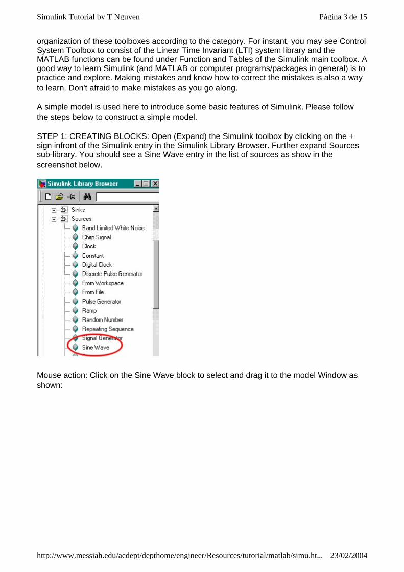
STEP 1: CREATING BLOCKS: Open (Expand) the Simulink toolbox by clicking on the + sign infront of the Simulink entry in the Simulink Library Browser. Further expand Sources sub-library. You should see a Sine Wave entry in the list of sources as show in the screenshot below.

Mouse action: Click on the Sine Wave block to select and drag it to the model Window as shown:



Now you have established a source of your model. In similar fashion, create additional blocks in your model window.

NOTE: It is advisable that you save your model at some point early on so that if your PC crashes (runing MATLAB under Linux OS is much more stable!) you don't loose so much time to reconstruct your model.

I am going to save this model under the filename: "simexample1". To save a model, go to the pulldown File menu in the model window and select Save As. A extension named ".mdl" will be automatically appended to the filename (just enter the filename). Simulink will recognize file with .mdl extension as a simulation model (similar to how MATLAB recognizes files with the extension .m as an MFile).

Continue to build your model by adding more components (or blocks) to your model window. We'll continue to add a scope from Sinks library, an Integrator block from Continuous library, and a Mux block from Signals & Systems library. Once all the blocks are dragged over to the model window, you would have a window that looks like one shown below.

You may remove a block that you don't want by clicking on the block to turn it to the select



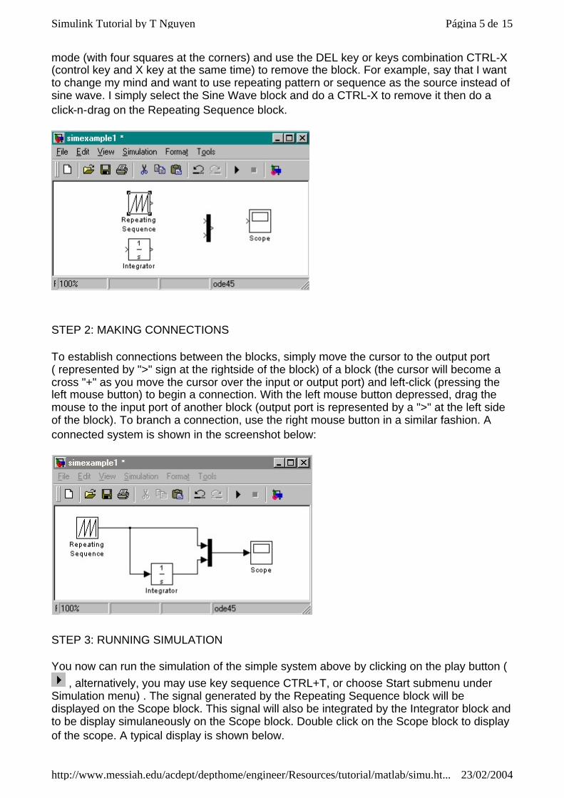
mode (with four squares at the corners) and use the DEL key or keys combination CTRL-X (control key and X key at the same time) to remove the block. For example, say that I want to change my mind and want to use repeating pattern or sequence as the source instead of sine wave. I simply select the Sine Wave block and do a CTRL-X to remove it then do a click-n-drag on the Repeating Sequence block.

STEP 2: MAKING CONNECTIONS

To establish connections between the blocks, simply move the cursor to the output port ( represented by ">" sign at the rightside of the block) of a block (the cursor will become a cross "+" as you move the cursor over the input or output port) and left-click (pressing the left mouse button) to begin a connection. With the left mouse button depressed, drag the mouse to the input port of another block (output port is represented by a ">" at the left side of the block). To branch a connection, use the right mouse button in a similar fashion. A connected system is shown in the screenshot below:

STEP 3: RUNNING SIMULATION

You now can run the simulation of the simple system above by clicking on the play button ( , alternatively, you may use key sequence CTRL+T, or choose Start submenu under

Simulation menu) . The signal generated by the Repeating Sequence block will be displayed on the Scope block. This signal will also be integrated by the Integrator block and to be display simulaneously on the Scope block. Double click on the Scope block to display of the scope. A typical display is shown below.



Note that if the derivative of the signal can be obtained using the Derivative block instead of the Integrator block. The result would be

as expected.

The above steps demonstrated some basic functions and structure of Simulink. It is strongly recommended that you take some time to explore the toolboxes and familiarize yourself with the parameters associated with each block. To view/edit the parameters, simply double click on the block of interest.

Handling of Blocks and Lines

The table below describes the actions and the corresponding keystrokes or mouse operations (Windows versions). Actions Keystokes or Mouse Actions

Copying a block from a library

Drag the block to the model window with the left button on the mouse OR use select the COPY and PASTE from EDIT menu.



Annotations

To add an annotation to your model, place the cursor at an unoccupied area in your model window and double click on the left mouse button. A small rectangular area will appear with a cursor prompting for your input.

To delete an annotation, hold down the SHIFT key while selecting the annotation, then press the DELETE or BACKSPACE key. You may also change font type and color from the FORMAT menu.

Some Examples

Example 1. Simulation of an Equation.

In this example we will use Simulink to model an equation. Let's consider...

where the displacement x is a function of time t, frequency w, phase angle phi, and amplitue A. In this example the values for these parameters are set as follows: frequency=5 rad/sec;phase=pi/2;A=2.

1. From Simulink's library drag the following blocks to the model window

Duplicating blocks in a model

Hold down the CTRL key and select the block with the left mouse drag the block to a new location.

Display block's paramters Double click on the blockFlip a block CTRL-FRotate a block (clockwise 90 deg @ each keystroke)

CTRL-R

Changing blocks' names Click on block's label and position the cursor to desired place.

Disconnecting a block hold down the SHIFT key and drag the block to a new location

Drawing a diagonal line hold down the SHIFT key while dragging the mouse with the left button

Dividing a line move the cursor to the line to where you want to creat the vertex and use the left button on the mouse to drag the line while holding down the SHIFT key

, (1)

Blocks to be dragged to the model window

Where located in Simulink library browser

Ramp Sources

Constant Sources

Gain Math



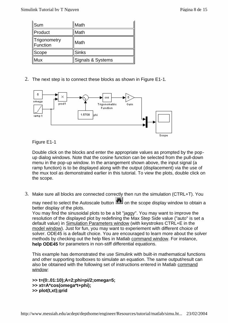
2. The next step is to connect these blocks as shown in Figure E1-1.

Figure E1-1 Double click on the blocks and enter the appropriate values as prompted by the pop-up dialog windows. Note that the cosine function can be selected from the pull-down menu in the pop-up window. In the arrangement shown above, the input signal (a ramp function) is to be displayed along with the output (displacement) via the use of the mux tool as demonstrated earlier in this tutorial. To view the plots, double click on the scope.

3. Make sure all blocks are connected correctly then run the simulation (CTRL+T). You

may need to select the Autoscale button on the scope display window to obtain a better display of the plots. You may find the sinusoidal plots to be a bit "jaggy". You may want to improve the resolution of the displayed plot by redefining the Max Step Side value ("auto" is set a default value) in Simulation Parameters window (with keystrokes CTRL+E in the model window). Just for fun, you may want to experiement with different choice of solver. ODE45 is a default choice. You are encouraged to learn more about the solver methods by checking out the help files in Matlab command window. For instance, help ODE45 for parameters in non-stiff differential equations. This example has demonstrated the use Simulink with built-in mathematical functions and other supporting toolboxes to simulate an equation. The same output/result can also be obtained with the following set of instructions entered in Matlab command window: >> t=(0:.01:10);A=2;phi=pi/2;omega=5; >> xt=A*cos(omega*t+phi); >> plot(t,xt);grid

Sum Math

Product Math

Trigonometry Function Math

Scope Sinks

Mux Signals & Systems



______________________________________

Example 2. Mass-Spring-Dashpot System Simulation

Figure E2-1

Consider a mass-spring-dashpot system as shown in Figure E2-1. The mathematical model for this system is described by

where m is the equivalent mass of the system, c is the damping ratio, k is the spring stiffness, and f(t) is the forcing function in the x-direction.

In this example will illustrate how to use Simulink to simulate the response of this system to unit step input.

, (2)

STEP 1

In Simulink, create a new model window (CTRL+N) and drag the following blocks from the Simulink library window:

Blocks to be dragged to the model window

Where located in Simulink library browser

Step Sources

Gain Math

Sum Math

Integrator Continuous

Scope Sinks

To Workspace Sinks

STEP 2

By re-arrange Eqn 2 to yield an expression for the acceleration term as

Based on Eqn 3, we connect the blocks in the diagram as shown in Figure E2-2. Use CTRL+F and CTRL+R to flip and rotate the blocks as necessary (select the block first then execute the key sequence). Note that you can use CTRL+right mouse button to create branches of the connecting lines. Don't worry about the parameter values and the signs for these blocks at this point as we'll take care of this in STEP 3. Just get them connected first.

(3)



Figure E2-2

STEP 3

Enter the values of the parameters for each block. In this example, we will set m = 2.0; c=0.7; k=1. You are encouraged to try different values and observe the system's response to step input.

To show that you may obtain different form of output, I included another block (in addition to the scope block) called "simout". This block can be found in the Sinks group from the Simulink Library browser. The output from this block is used in Matlab workspace. To illustrate how this block works, I will select a name for the output called "simout" as the variable name in the block's parameter setting (double click on the "simput" block to bring up the parameter dialog window). In additon, I will need a time array from the simulation. This can be specifed as a parameter in the Simulation Parameter window (CTRL+E) under the Workspace I/O tab as shown in Figure E2-3.

Figure E2-3

STEP 4

Run the simulation by clicking on the button (alternately you may use keyboard command CTRL+T ). The screenshot of the output from the Scope block is show in Figure E2-3.



Example 3. Using the same system presented in Example 2, we will simulate the response using transfer function block (frequency domain). This example will illustrate an alternate approach to one shown above.

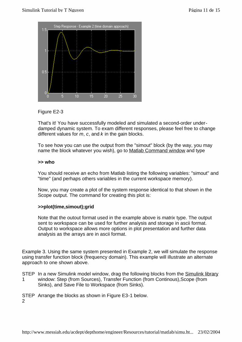
Figure E2-3

That's it! You have successfully modeled and simulated a second-order under-damped dynamic system. To exam different responses, please feel free to change different values for m, c, and k in the gain blocks.

To see how you can use the output from the "simout" block (by the way, you may name the block whatever you wish), go to Matlab Command window and type

>> who

You should receive an echo from Matlab listing the following variables: "simout" and "time" (and perhaps others variables in the current workspace memory).

Now, you may create a plot of the system response identical to that shown in the Scope output. The command for creating this plot is:

>>plot(time,simout);grid

Note that the outout format used in the example above is matrix type. The output sent to workspace can be used for further analysis and storage in ascii format. Output to workspace allows more options in plot presentation and further data analysis as the arrays are in ascii format.

STEP 1

In a new Simulink model window, drag the following blocks from the Simulink library window: Step (from Sources), Transfer Function (from Continous),Scope (from Sinks), and Save File to Workspace (from Sinks).

STEP 2

Arrange the blocks as shown in Figure E3-1 below.



Figure E3-1

STEP 3

Entering blocks' parameters values.

We'll use the same values for m, c, and k as in Example 2. Double click on the transfer function to bring up the parameter diaglog window and enter the values for the coefficients in the denominator as shown in Figure E3-2. Note that the Transfer function block has a defaut form of first order in the denominator (s+1). You may specify different order for the numerator and the denominator by entering the coefficients associated with the polynomials.

Figure E3-2

Click OK to close the dialog.

Double click on the Save Output To A File block to open the dialog window as shown in Figure E3-3. In the Filename box specify the path and the name of the file you wish to save. The saved file will be in .MAT format (yes, it's in binary format! So don't try to read it). You will be able to load this file to Matlab workspace later on. Make sure to remember where you save the file to. In this example, I'll put the file in my D drive under "temp" directory and name the file "example3out.mat". You may choose other convenient location on your computer.

In the Variable name box, enter a name of your choice. Here I name the variable "simout".



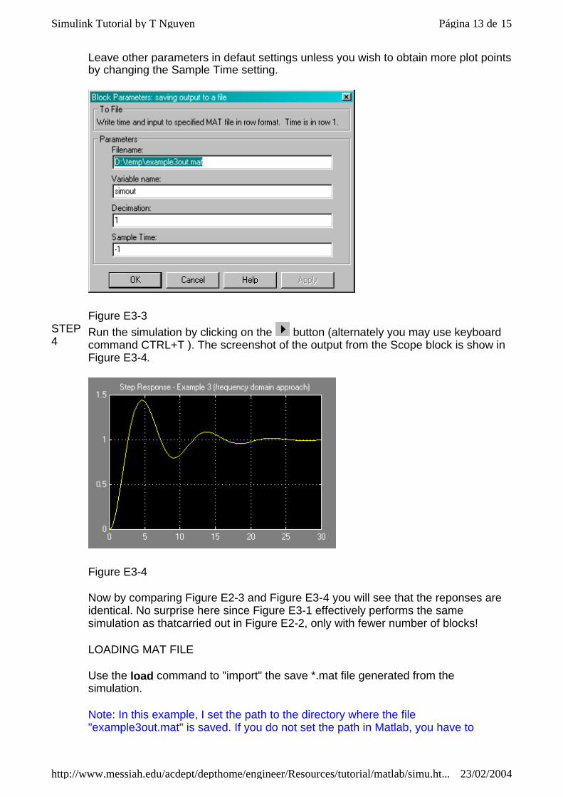
Leave other parameters in defaut settings unless you wish to obtain more plot points by changing the Sample Time setting.

Figure E3-3 STEP 4

Run the simulation by clicking on the button (alternately you may use keyboard command CTRL+T ). The screenshot of the output from the Scope block is show in Figure E3-4.

Figure E3-4

Now by comparing Figure E2-3 and Figure E3-4 you will see that the reponses are identical. No surprise here since Figure E3-1 effectively performs the same simulation as thatcarried out in Figure E2-2, only with fewer number of blocks!

LOADING MAT FILE

Use the load command to "import" the save *.mat file generated from the simulation.

Note: In this example, I set the path to the directory where the file "example3out.mat" is saved. If you do not set the path in Matlab, you have to



specify the full path in the load command,e.g.,>>load D:/temp/example3out.mat .

In Matlab command window, enter the followings:

>> load example3out

You may want to verify the loading by asking Matlab to list all of the variables in the current workspace:

>> who

If the loading is successful, you should see the variable you specified earlier listed the current workspace. In this example, Matlab echos:

Your variables are:

simout

"simout" is a 2 x m matrix, where m is number of columns reflecting the number of data points generated from the simulation. The first row contains the time array.

To generate a plot of the step input response from the simulation, simply use the plot command on "simout" matrix. For this example, the following command produces the plot shown in Figure E3-5.

>> plot(simout(1,:),simout(2,:));grid

Figure E3-5

In summary, the simulations of a second-order continuous system modeled by Equation 2 have been shown using two different approaches. Different file output options from Simulink were also demonstrated.

____________________________________________________________

MORE EXAMPLE WILL BE ADDED...



[ BACK TO TOP ]

References and further readings:

1. Matlab help files 2. Mathworks' documentations on Simulink



part two: simulink getting started · steps in using simulink. though this tutorial covers the...

Documents