SIMULINK A Tutorial by Tom Nguyen

Introduction

Simulink (Simulation and Link) is an extension of MATLAB by Mathworks Inc. Itworks with MATLAB to offer modeling, simulating, and analyzing of dynamicalsystems under a graphical user interface (GUI) environment. The construction of amodel is simplified with click-and-drag mouse operations. Simulink includes acomprehensive block library of toolboxes for both linear and nonlinear analyses.Models are hierarchical, which allow using both top-down and bottom-upapproaches. As Simulink is an integral part of MATLAB, it is easy to switch back andforth during the analysis process and thus, the user may take full advantage offeatures offered in both environments. This tutorial presents the basic features ofSimulink and is focused on control systems as it has been written for students inmy control systems course.

This tutorial has been written for Simulink v.5 and v.6. Getting Started

To start a Simulink session, you'd need to bring up Matlab program first.

From Matlab command window, enter:

>> simulink

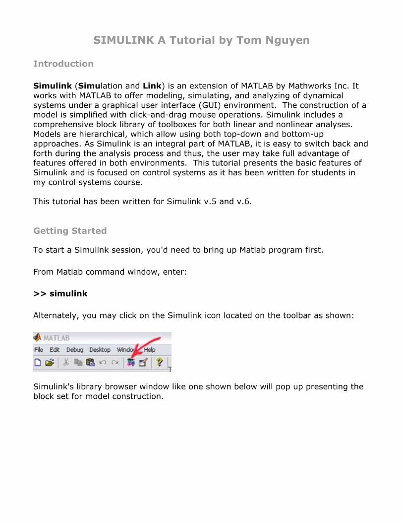
Alternately, you may click on the Simulink icon located on the toolbar as shown:

Simulink's library browser window like one shown below will pop up presenting theblock set for model construction.

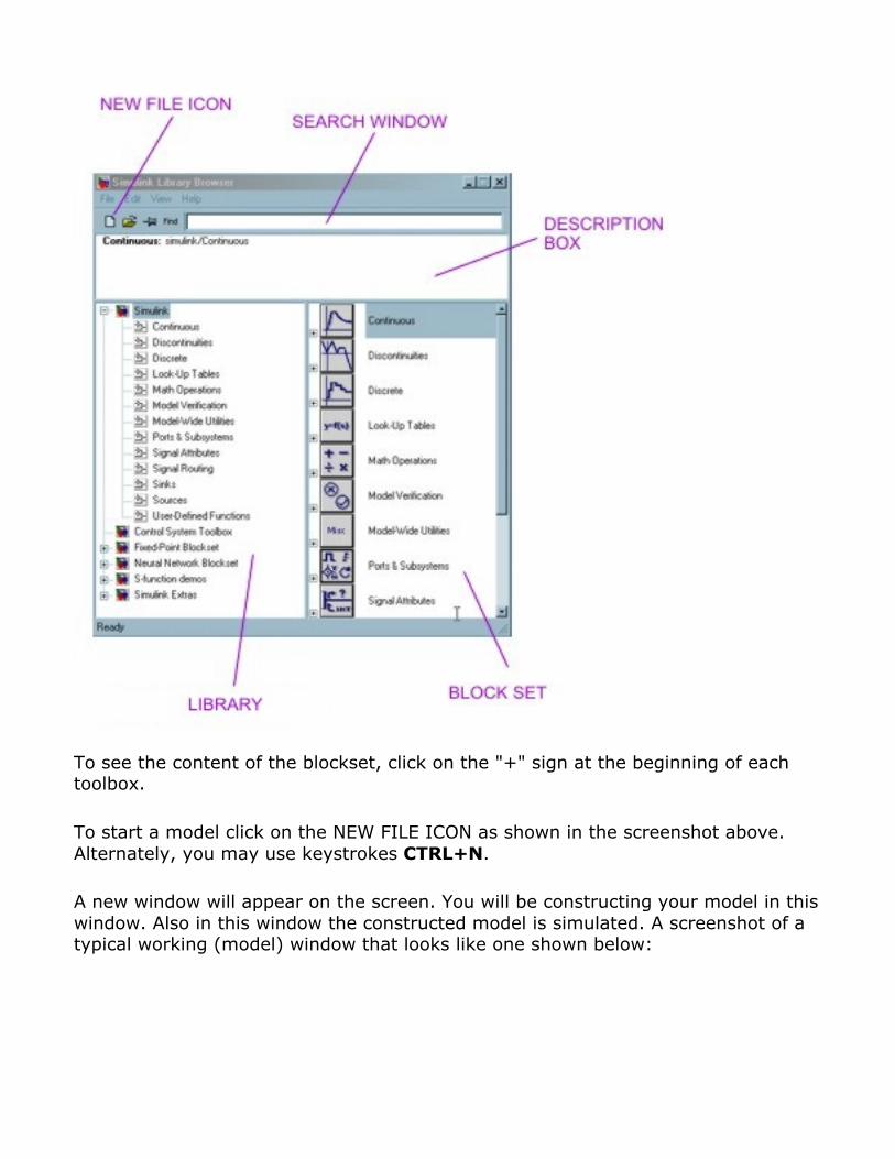
To see the content of the blockset, click on the "+" sign at the beginning of eachtoolbox.

To start a model click on the NEW FILE ICON as shown in the screenshot above.Alternately, you may use keystrokes CTRL+N.

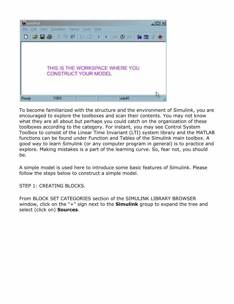
A new window will appear on the screen. You will be constructing your model in thiswindow. Also in this window the constructed model is simulated. A screenshot of atypical working (model) window that looks like one shown below:

To become familiarized with the structure and the environment of Simulink, you areencouraged to explore the toolboxes and scan their contents. You may not knowwhat they are all about but perhaps you could catch on the organization of thesetoolboxes according to the category. For instant, you may see Control SystemToolbox to consist of the Linear Time Invariant (LTI) system library and the MATLABfunctions can be found under Function and Tables of the Simulink main toolbox. Agood way to learn Simulink (or any computer program in general) is to practice andexplore. Making mistakes is a part of the learning curve. So, fear not, you shouldbe.

A simple model is used here to introduce some basic features of Simulink. Pleasefollow the steps below to construct a simple model.

STEP 1: CREATING BLOCKS.

From BLOCK SET CATEGORIES section of the SIMULINK LIBRARY BROWSERwindow, click on the "+" sign next to the Simulink group to expand the tree andselect (click on) Sources.

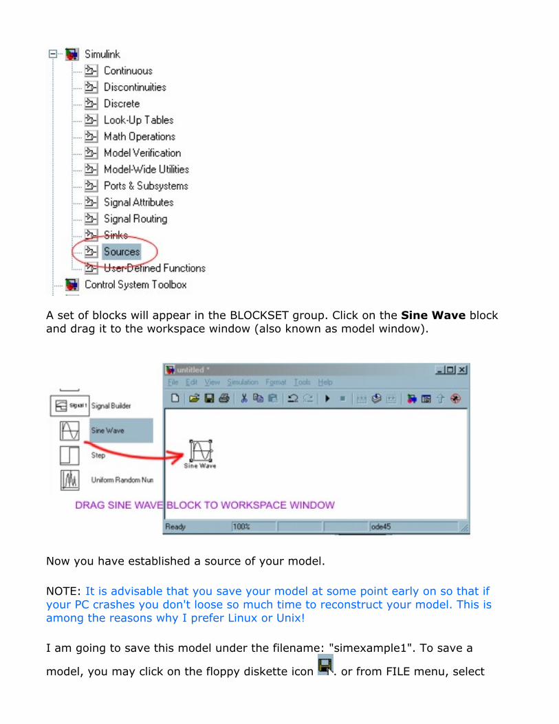
A set of blocks will appear in the BLOCKSET group. Click on the Sine Wave blockand drag it to the workspace window (also known as model window).

Now you have established a source of your model.

NOTE: It is advisable that you save your model at some point early on so that ifyour PC crashes you don't loose so much time to reconstruct your model. This isamong the reasons why I prefer Linux or Unix!

I am going to save this model under the filename: "simexample1". To save a

model, you may click on the floppy diskette icon . or from FILE menu, select

Save or CTRL+S. All Simulink model file will have an extension ".mdl". Simulinkrecognizes file with .mdl extension as a simulation model (similar to how MATLABrecognizes files with the extension .m as an MFile).

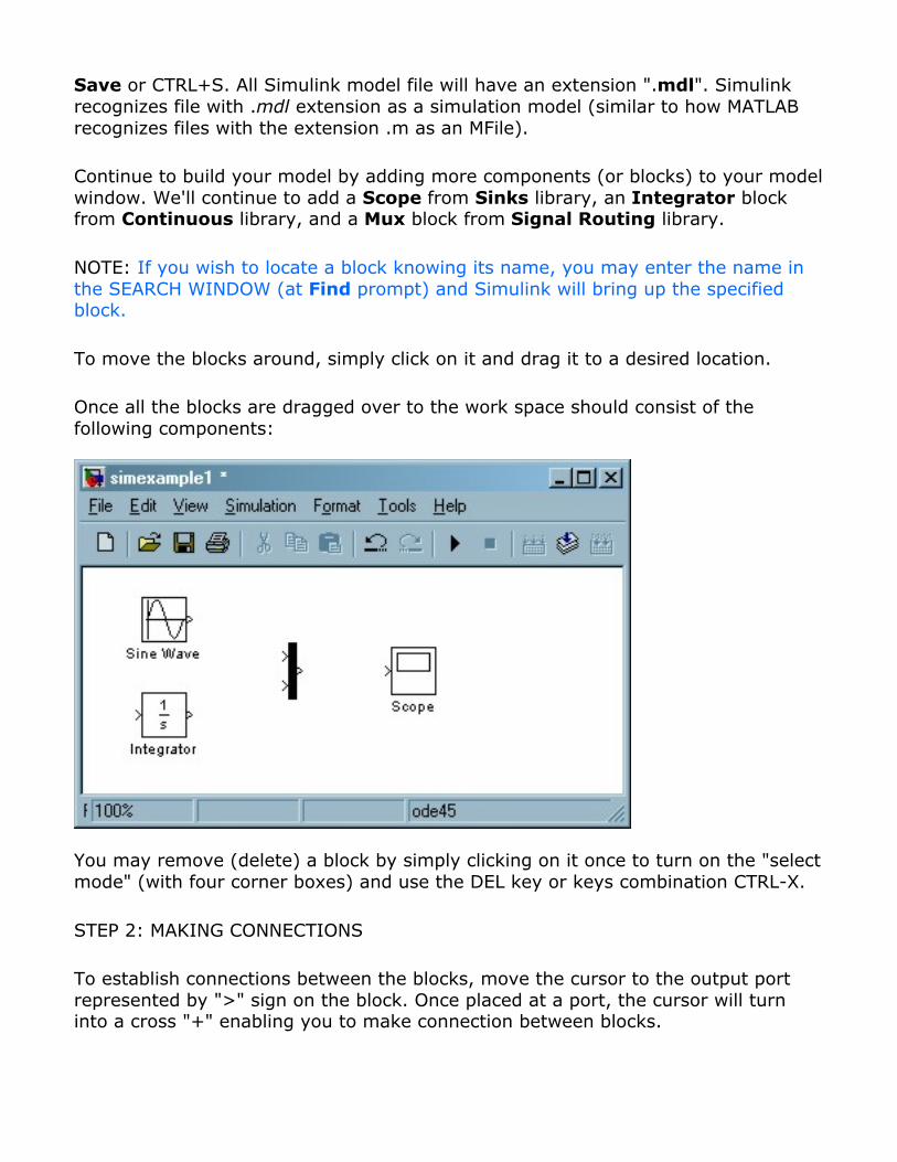
Continue to build your model by adding more components (or blocks) to your modelwindow. We'll continue to add a Scope from Sinks library, an Integrator blockfrom Continuous library, and a Mux block from Signal Routing library.

NOTE: If you wish to locate a block knowing its name, you may enter the name inthe SEARCH WINDOW (at Find prompt) and Simulink will bring up the specifiedblock.

To move the blocks around, simply click on it and drag it to a desired location.

Once all the blocks are dragged over to the work space should consist of thefollowing components:

You may remove (delete) a block by simply clicking on it once to turn on the "selectmode" (with four corner boxes) and use the DEL key or keys combination CTRL-X.

STEP 2: MAKING CONNECTIONS

To establish connections between the blocks, move the cursor to the output portrepresented by ">" sign on the block. Once placed at a port, the cursor will turninto a cross "+" enabling you to make connection between blocks.

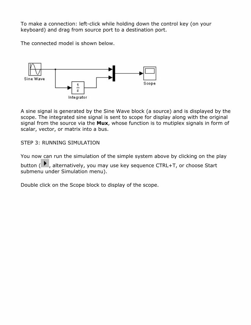
To make a connection: left-click while holding down the control key (on yourkeyboard) and drag from source port to a destination port.

The connected model is shown below.

A sine signal is generated by the Sine Wave block (a source) and is displayed by thescope. The integrated sine signal is sent to scope for display along with the originalsignal from the source via the Mux, whose function is to mutiplex signals in form ofscalar, vector, or matrix into a bus.

STEP 3: RUNNING SIMULATION

You now can run the simulation of the simple system above by clicking on the play

button ( , alternatively, you may use key sequence CTRL+T, or choose Startsubmenu under Simulation menu).

Double click on the Scope block to display of the scope.

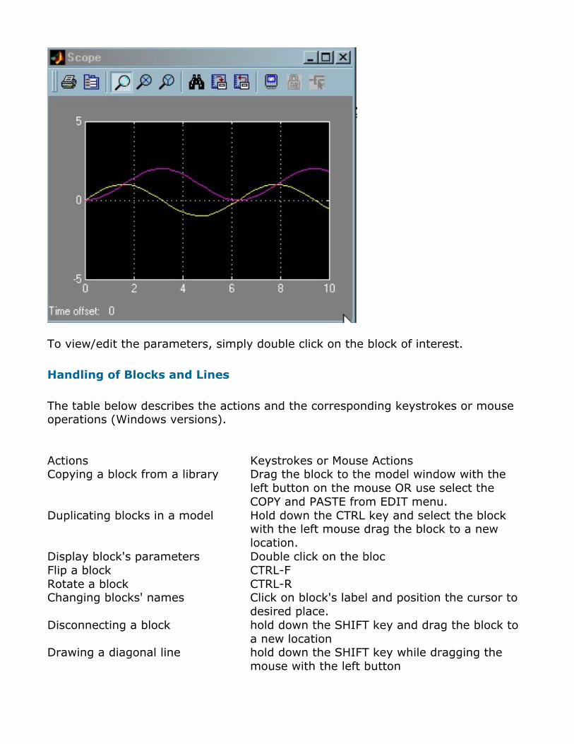
To view/edit the parameters, simply double click on the block of interest.

Handling of Blocks and Lines

The table below describes the actions and the corresponding keystrokes or mouseoperations (Windows versions). Actions Keystrokes or Mouse ActionsCopying a block from a library Drag the block to the model window with the

left button on the mouse OR use select theCOPY and PASTE from EDIT menu.

Duplicating blocks in a model Hold down the CTRL key and select the blockwith the left mouse drag the block to a newlocation.

Display block's parameters Double click on the blocFlip a block CTRL-FRotate a block CTRL-RChanging blocks' names Click on block's label and position the cursor to

desired place.Disconnecting a block hold down the SHIFT key and drag the block to

a new locationDrawing a diagonal line hold down the SHIFT key while dragging the

mouse with the left button

Dividing a line move the cursor to the line to where you wantto create the vertex and use the left button onthe mouse to drag the line while holding downthe SHIFT key

Annotations

To add an annotation to your model, place the cursor at an unoccupied area in yourmodel window and double click (left button). A small rectangular area will appearwith a cursor prompting for your input.

To delete an annotation, hold down the SHIFT key while selecting the annotation,then press the DELETE or BACKSPACE key. You may also change font type andcolor from the FORMAT menu.

SIMULINK EXAMPLES

Example 1. Simulation of an Equation.

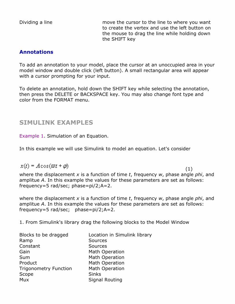
In this example we will use Simulink to model an equation. Let's consider

(1)where the displacement x is a function of time t, frequency w, phase angle phi, andamplitue A. In this example the values for these parameters are set as follows:frequency=5 rad/sec; phase=pi/2;A=2.

where the displacement x is a function of time t, frequency w, phase angle phi, andamplitue A. In this example the values for these parameters are set as follows:frequency=5 rad/sec; phase=pi/2;A=2.

1. From Simulink's library drag the following blocks to the Model Window

Blocks to be dragged Location in Simulink libraryRamp SourcesConstant SourcesGain Math OperationSum Math OperationProduct Math OperationTrigonometry Function Math OperationScope SinksMux Signal Routing

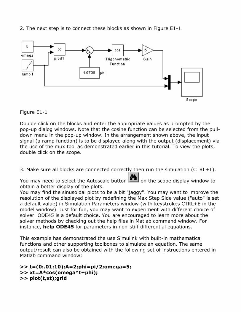
2. The next step is to connect these blocks as shown in Figure E1-1.

Figure E1-1

Double click on the blocks and enter the appropriate values as prompted by thepop-up dialog windows. Note that the cosine function can be selected from the pull-down menu in the pop-up window. In the arrangement shown above, the inputsignal (a ramp function) is to be displayed along with the output (displacement) viathe use of the mux tool as demonstrated earlier in this tutorial. To view the plots,double click on the scope.

3. Make sure all blocks are connected correctly then run the simulation (CTRL+T).

You may need to select the Autoscale button on the scope display window toobtain a better display of the plots.You may find the sinusoidal plots to be a bit "jaggy". You may want to improve theresolution of the displayed plot by redefining the Max Step Side value ("auto" is seta default value) in Simulation Parameters window (with keystrokes CTRL+E in themodel window). Just for fun, you may want to experiment with different choice ofsolver. ODE45 is a default choice. You are encouraged to learn more about thesolver methods by checking out the help files in Matlab command window. Forinstance, help ODE45 for parameters in non-stiff differential equations.

This example has demonstrated the use Simulink with built-in mathematicalfunctions and other supporting toolboxes to simulate an equation. The sameoutput/result can also be obtained with the following set of instructions entered inMatlab command window:

>> t=(0:.01:10);A=2;phi=pi/2;omega=5;>> xt=A*cos(omega*t+phi);>> plot(t,xt);grid

Example 2. Mass-Spring-Dashpot System Simulation

Consider a mass-spring-dashpot system where the spring and the dashpot areconnected in parallel to the mass. The mathematical model for this system isdescribed by

(2)In this example I will illustrate how to use Simulink to simulate the response of thissystem to unit step input.

STEP 1In Simulink, create a new model window (CTRL+N) and drag the following blocksfrom the Simulink library window:

Blocks to be dragged Location in Simulink library browserStep SourcesGain Math OperationSum Math OperationIntegrator ContinuousScope SinksTo Workspace Sinks

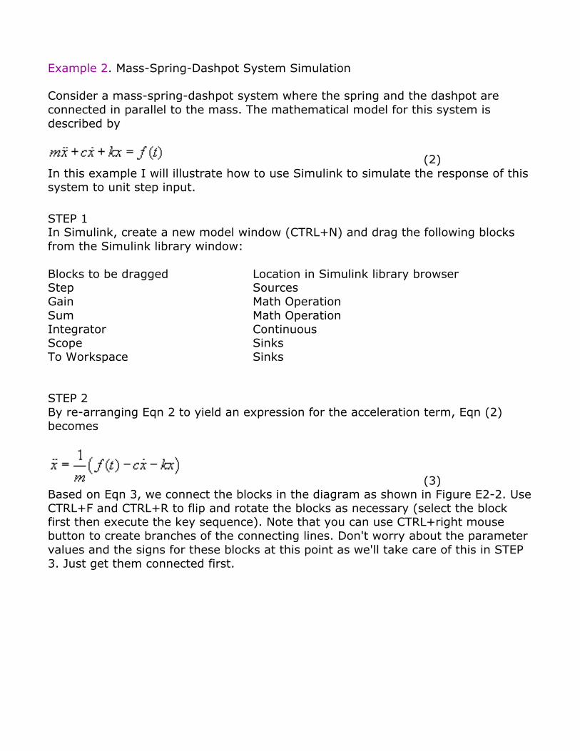
STEP 2 By re-arranging Eqn 2 to yield an expression for the acceleration term, Eqn (2)becomes

(3)Based on Eqn 3, we connect the blocks in the diagram as shown in Figure E2-2. UseCTRL+F and CTRL+R to flip and rotate the blocks as necessary (select the blockfirst then execute the key sequence). Note that you can use CTRL+right mousebutton to create branches of the connecting lines. Don't worry about the parametervalues and the signs for these blocks at this point as we'll take care of this in STEP3. Just get them connected first.

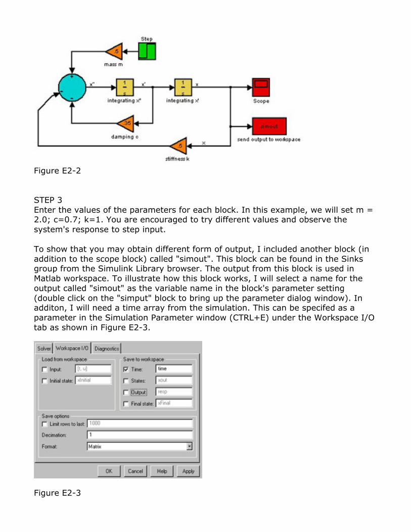
Figure E2-2

STEP 3Enter the values of the parameters for each block. In this example, we will set m =2.0; c=0.7; k=1. You are encouraged to try different values and observe thesystem's response to step input.

To show that you may obtain different form of output, I included another block (inaddition to the scope block) called "simout". This block can be found in the Sinksgroup from the Simulink Library browser. The output from this block is used inMatlab workspace. To illustrate how this block works, I will select a name for theoutput called "simout" as the variable name in the block's parameter setting(double click on the "simput" block to bring up the parameter dialog window). Inadditon, I will need a time array from the simulation. This can be specifed as aparameter in the Simulation Parameter window (CTRL+E) under the Workspace I/Otab as shown in Figure E2-3.

Figure E2-3

STEP 4

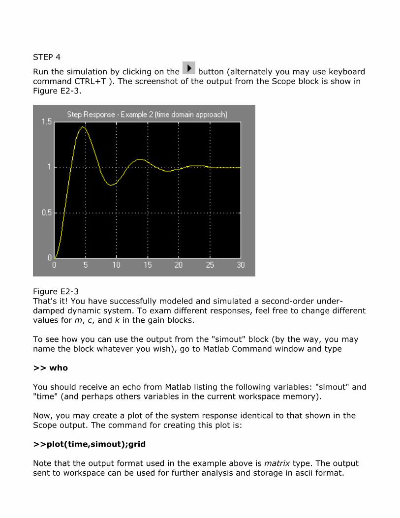
Run the simulation by clicking on the button (alternately you may use keyboardcommand CTRL+T ). The screenshot of the output from the Scope block is show inFigure E2-3.

Figure E2-3That's it! You have successfully modeled and simulated a second-order under-damped dynamic system. To exam different responses, feel free to change differentvalues for m, c, and k in the gain blocks.

To see how you can use the output from the "simout" block (by the way, you mayname the block whatever you wish), go to Matlab Command window and type

>> who

You should receive an echo from Matlab listing the following variables: "simout" and"time" (and perhaps others variables in the current workspace memory).

Now, you may create a plot of the system response identical to that shown in theScope output. The command for creating this plot is:

>>plot(time,simout);grid

Note that the output format used in the example above is matrix type. The outputsent to workspace can be used for further analysis and storage in ascii format.

Output to workspace allows more options in plot presentation and further dataanalysis as the arrays are in ascii format.

Example 3. Using the same system presented in Example 2, we will simulate theresponse using transfer function approach.

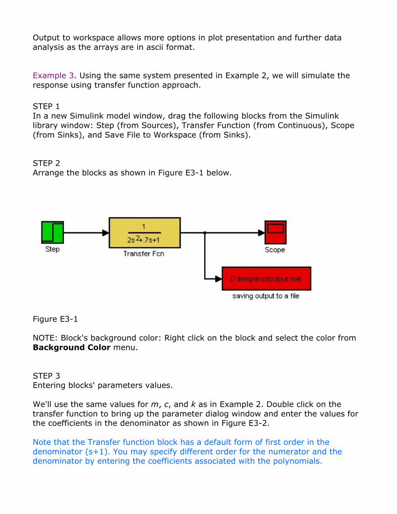
STEP 1In a new Simulink model window, drag the following blocks from the Simulinklibrary window: Step (from Sources), Transfer Function (from Continuous), Scope(from Sinks), and Save File to Workspace (from Sinks).

STEP 2 Arrange the blocks as shown in Figure E3-1 below.

Figure E3-1

NOTE: Block's background color: Right click on the block and select the color fromBackground Color menu.

STEP 3Entering blocks' parameters values.

We'll use the same values for m, c, and k as in Example 2. Double click on thetransfer function to bring up the parameter dialog window and enter the values forthe coefficients in the denominator as shown in Figure E3-2.

Note that the Transfer function block has a default form of first order in thedenominator (s+1). You may specify different order for the numerator and thedenominator by entering the coefficients associated with the polynomials.

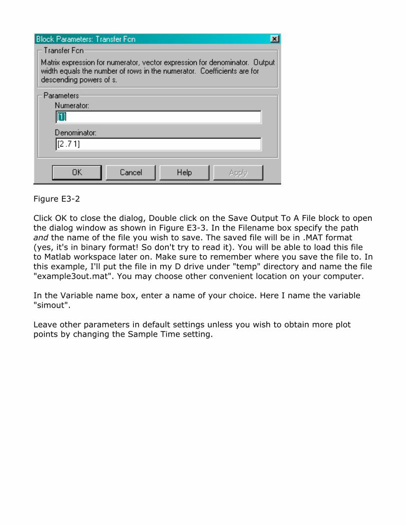
Figure E3-2

Click OK to close the dialog, Double click on the Save Output To A File block to openthe dialog window as shown in Figure E3-3. In the Filename box specify the pathand the name of the file you wish to save. The saved file will be in .MAT format(yes, it's in binary format! So don't try to read it). You will be able to load this fileto Matlab workspace later on. Make sure to remember where you save the file to. Inthis example, I'll put the file in my D drive under "temp" directory and name the file"example3out.mat". You may choose other convenient location on your computer.

In the Variable name box, enter a name of your choice. Here I name the variable"simout".

Leave other parameters in default settings unless you wish to obtain more plotpoints by changing the Sample Time setting.

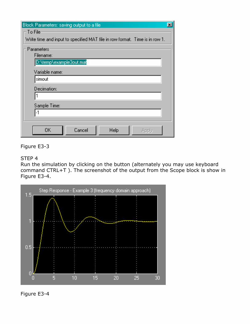
Figure E3-3

STEP 4Run the simulation by clicking on the button (alternately you may use keyboardcommand CTRL+T ). The screenshot of the output from the Scope block is show inFigure E3-4.

Figure E3-4

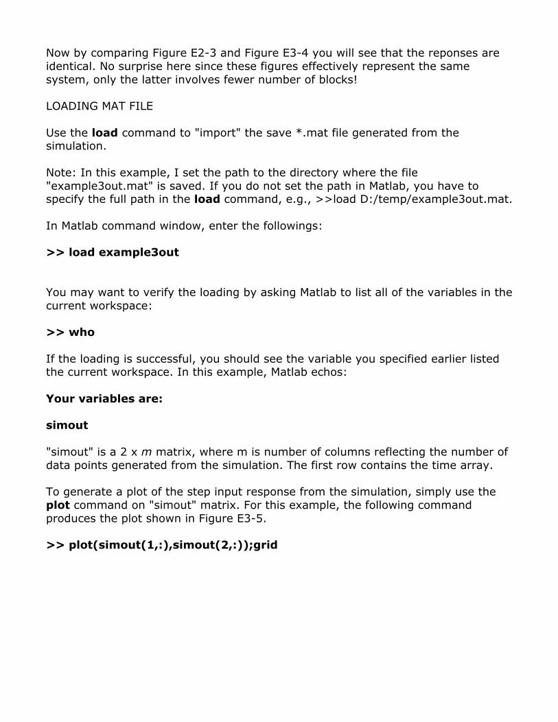
Now by comparing Figure E2-3 and Figure E3-4 you will see that the reponses areidentical. No surprise here since these figures effectively represent the samesystem, only the latter involves fewer number of blocks!

LOADING MAT FILE

Use the load command to "import" the save *.mat file generated from thesimulation.

Note: In this example, I set the path to the directory where the file"example3out.mat" is saved. If you do not set the path in Matlab, you have tospecify the full path in the load command, e.g., >>load D:/temp/example3out.mat.

In Matlab command window, enter the followings:

>> load example3out

You may want to verify the loading by asking Matlab to list all of the variables in thecurrent workspace:

>> who

If the loading is successful, you should see the variable you specified earlier listedthe current workspace. In this example, Matlab echos:

Your variables are:

simout

"simout" is a 2 x m matrix, where m is number of columns reflecting the number ofdata points generated from the simulation. The first row contains the time array.

To generate a plot of the step input response from the simulation, simply use theplot command on "simout" matrix. For this example, the following commandproduces the plot shown in Figure E3-5.

>> plot(simout(1,:),simout(2,:));grid

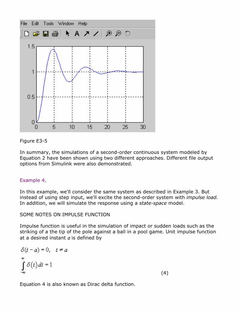
Figure E3-5

In summary, the simulations of a second-order continuous system modeled byEquation 2 have been shown using two different approaches. Different file outputoptions from Simulink were also demonstrated.

Example 4.

In this example, we'll consider the same system as described in Example 3. Butinstead of using step input, we'll excite the second-order system with impulse load.In addition, we will simulate the response using a state-space model.

SOME NOTES ON IMPULSE FUNCTION

Impulse function is useful in the simulation of impact or sudden loads such as thestriking of a the tip of the pole against a ball in a pool game. Unit impulse functionat a desired instant a is defined by

(4)

Equation 4 is also known as Dirac delta function.

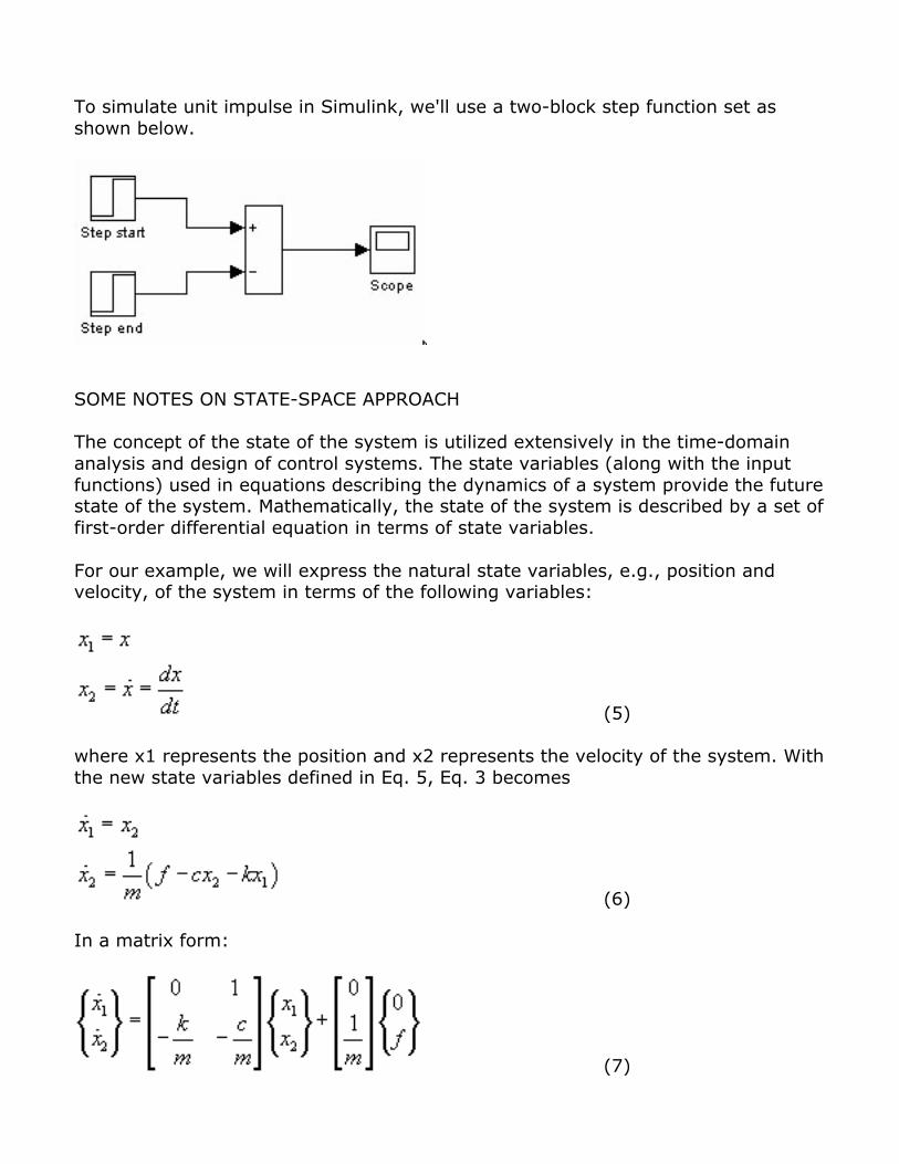
To simulate unit impulse in Simulink, we'll use a two-block step function set asshown below.

SOME NOTES ON STATE-SPACE APPROACH

The concept of the state of the system is utilized extensively in the time-domainanalysis and design of control systems. The state variables (along with the inputfunctions) used in equations describing the dynamics of a system provide the futurestate of the system. Mathematically, the state of the system is described by a set offirst-order differential equation in terms of state variables.

For our example, we will express the natural state variables, e.g., position andvelocity, of the system in terms of the following variables:

(5)

where x1 represents the position and x2 represents the velocity of the system. Withthe new state variables defined in Eq. 5, Eq. 3 becomes

(6)

In a matrix form:

(7)

Equation 7 may be expressed in a more compact form:

(8)

where A is known as the system matrix and B as the input matrix.The output equation is expressed by

(9)where

(10)and

(11)

C is called the output matrix and D is called the direct transmittance matrix.

MATLAB AND SIMULINK APPLICATION

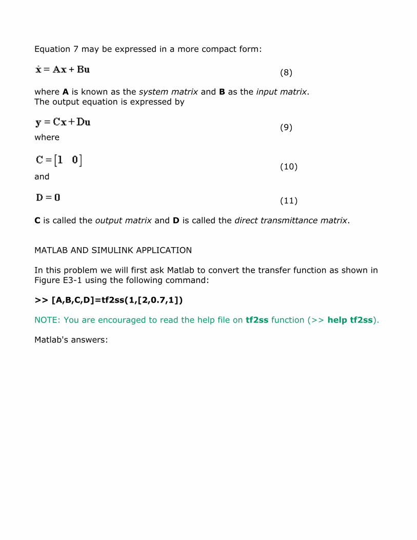
In this problem we will first ask Matlab to convert the transfer function as shown inFigure E3-1 using the following command:

>> [A,B,C,D]=tf2ss(1,[2,0.7,1])

NOTE: You are encouraged to read the help file on tf2ss function (>> help tf2ss).

Matlab's answers:

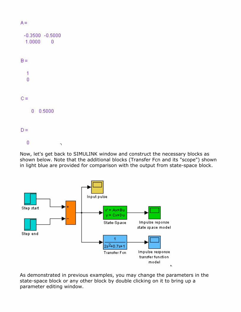
Now, let's get back to SIMULINK window and construct the necessary blocks asshown below. Note that the additional blocks (Transfer Fcn and its "scope") shownin light blue are provided for comparison with the output from state-space block.

As demonstrated in previous examples, you may change the parameters in thestate-space block or any other block by double clicking on it to bring up aparameter editing window.

For state space model, enter the following parameters:

A: [-0.35 -0.5;1 0]B: [1;0]C: [0 0.5]D: 0

Once the entries are completed, click OK button to close the panel and continue onmaking necessary entries for other blocks.

For the impulse simulation:

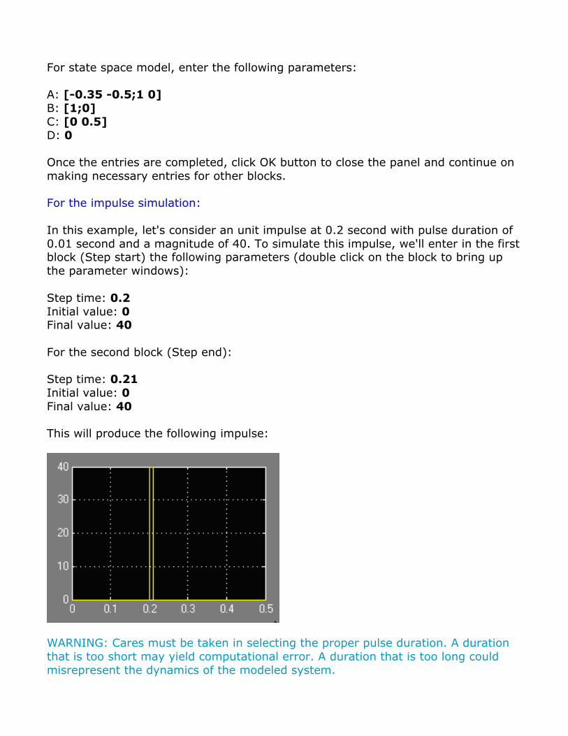
In this example, let's consider an unit impulse at 0.2 second with pulse duration of0.01 second and a magnitude of 40. To simulate this impulse, we'll enter in the firstblock (Step start) the following parameters (double click on the block to bring upthe parameter windows):

Step time: 0.2Initial value: 0Final value: 40

For the second block (Step end):

Step time: 0.21Initial value: 0Final value: 40

This will produce the following impulse:

WARNING: Cares must be taken in selecting the proper pulse duration. A durationthat is too short may yield computational error. A duration that is too long couldmisrepresent the dynamics of the modeled system.

To run the simulation use keystrokes: CTRL+T or click on the button.

To change the simulation parameters and make adjustment to simulation duration,press CTRL+E or choose Simulation parameters... from Simulation menu.

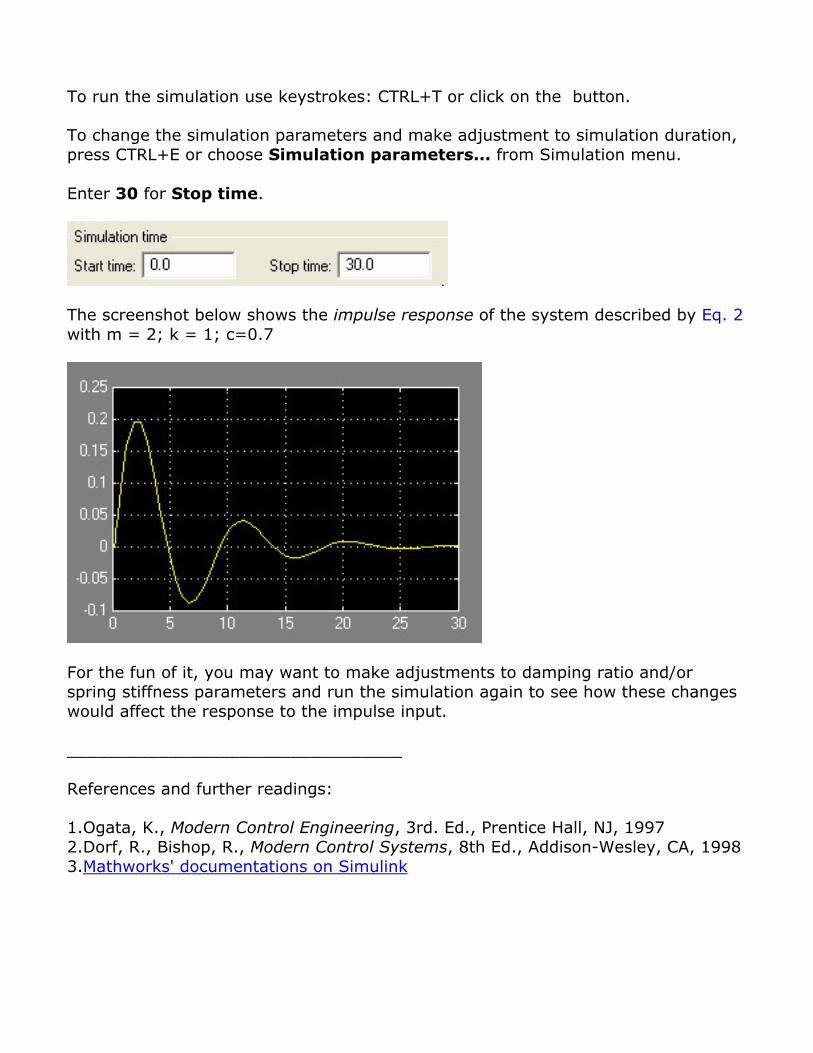
Enter 30 for Stop time.

The screenshot below shows the impulse response of the system described by Eq. 2with m = 2; k = 1; c=0.7

For the fun of it, you may want to make adjustments to damping ratio and/orspring stiffness parameters and run the simulation again to see how these changeswould affect the response to the impulse input.

_________________________________

References and further readings:

1.Ogata, K., Modern Control Engineering, 3rd. Ed., Prentice Hall, NJ, 19972.Dorf, R., Bishop, R., Modern Control Systems, 8th Ed., Addison-Wesley, CA, 19983.Mathworks' documentations on Simulink