pasw categories 17.0 - spss · predict outcomes and reveal relationships in categorical data pasw®...
TRANSCRIPT

Predict Outcomes and Reveal Relationships in Categorical Data
PASW® Categories 17.0 – Specifications
Unleash the full potential of your data through predictive
analysis, statistical learning, perceptual mapping,
preference scaling, and dimension reduction techniques,
including optimal scaling of your variables. PASW
Categories* provides you with all the tools you need to
obtain clear insight into complex categorical and numeric
data, as well as high-dimensional data.
For example, use PASW Categories to understand which
characteristics consumers relate most closely to your
product or brand, or to determine customer perception
of your products compared to other products that you or
your competitors offer.
With PASW Categories, you can do regression when both
predictor and outcome variables are numeric, ordinal, or
nominal, and visually interpret data to see how rows and
columns relate in large tables of scores, counts, ratings,
rankings, or similarities. This gives you the ability to:
n Work with and understand ordinal and nominal
data using procedures similar to conventional
regression, principal components, and canonical
correlation analyses
n Deal with non-normal residuals in numeric data or
nonlinear relationships between predictor variables
and the outcome variable. Use the options for Ridge
Regression, the Lasso, the Elastic Net, variable
selection, and model selection for both numeric
and categorical data.
n Use biplots and triplots to represent the relationship
between objects (cases), categories, and (sets of)
variables in correlation analyses
n Represent similarities between one or two sets of
objects as distances in perceptual maps
Turn your qualitative variables into quantitative ones
The advanced procedures available in PASW Categories
enable you to perform additional statistical operations
on categorical data.
Use PASW Categories’ optimal scaling procedures to assign
units of measurement and zero-points to your categorical
data. This opens up a new set of statistical functions by
allowing you to perform analyses on variables of mixed
measurement levels—on combinations of nominal, ordinal,
and numeric variables, for example.
* PASW Categories and PASW Statistics Base, formerly called SPSS Categories™ and SPSS Statistics Base, are part of SPSS Inc.’s Predictive Analytics Software portfolio.
PASW Categories’ ability to perform multiple regression
with optimal scaling gives you the opportunity to apply
regression when you have mixtures of numerical, ordinal,
and nominal predictors and outcome variables. The latest
version of PASW Categories includes state-of-the-art
procedures for model selection and regularization. You
can perform correspondence and multiple correspondence
analyses to numerically evaluate the relationships between
two or more nominal variables in your data. You may also
use correspondence analysis to analyze any table with
nonnegative entries.
And, with its principal components analysis procedure, you
can reduce your data to important components. Biplots
and triplots of objects, categories, and variables show their
relationships. These options are also available for numeric
data. Optimal scaling gives you a correlation matrix based
on quantifications of your ordinal and nominal variables.
Or you can split your variables into sets, and then analyze
the relationships between the sets by using nonlinear
canonical correlation analysis.
Graphically display underlying relationships
Whatever types of categories you study—market segments,
medical diagnoses, subcultures, political parties, or
biological species—optimal scaling procedures free you
from the restrictions associated with two-way tables,
placing the relationships among your variables in a larger
frame of reference. You can see a map of your data—not
just a statistical report.
PASW Categories’ dimension reduction techniques enable
you to go beyond unwieldy tables. Instead, you can clarify
relationships in your data by using perceptual maps and
biplots.
nPerceptual maps are high-resolution summary charts
that graphically display similar variables or categories
close to each other. They provide you with unique
insight into relationships between more than two
categorical variables.
nBiplots and triplots enable you to look at the
relationships among cases, variables, and categories.
For example, you can define relationships between
products, customers, and demographic characteristics.
By using the preference scaling procedure, you can further
visualize relationships among objects. The breakthrough
unfolding algorithm on which this procedure is based
enables you to perform non-metric analyses for ordinal
data and obtain meaningful results. The proximities scaling
procedure allows you to analyze similarities between
objects, and incorporate characteristics for the objects in
the same analysis.
How you can use PASW Categories
The following procedures are available to add meaning to
your data analyses.
Categorical regression (CATREG) predicts the values of a
nominal, ordinal, or numerical outcome variable from a
combination of numeric and (un)ordered categorical
predictor variables. You can use regression with optimal
scaling to describe, for example, how job satisfaction can
be predicted from job category, geographic region, and the
amount of work-related travel.
Optimal scaling techniques quantify the variables in such a
way that the Multiple R is maximized. Optimal scaling may
be applied to numeric variables when the residuals are
non-normal or when the predictor variables are not linearly
related with the outcome variable. Three new regularization
methods: Ridge regression, the Lasso, and the Elastic Net,
improve prediction accuracy by stabilizing the parameter
estimates. Automatic variable selection makes it possible
to analyze high-volume datasets—more variables than
objects. And by using the numeric scaling level, you can
do regularization in regression by using the Lasso or the
Elastic Net for your numeric data as well.
You can also use CATREG to apply particular Generalized
Additive Models (GAM), both for your numeric and
categorical data.
Correspondence analysis (CORRESPONDENCE) enables you
to analyze two-way tables that contain some measurement
of correspondence between rows and columns, as well
as display rows and columns as points in a map. A very
common type of correspondence table is a crosstabulation
in which the cells contain joint frequency counts for two
nominal variables. PASW Categories displays relationships
among the categories of these nominal variables in a visual
presentation.
Multiple correspondence analysis (MULTIPLE
CORRESPONDENCE) differs from correspondence analysis
in that it allows you to use more than two variables in your
analysis. With this procedure, all the variables are analyzed
at the nominal level (unordered categories).
For example, you can use multiple correspondence analysis
to explore relationships between favorite television show,
age group, and gender. By examining a low-dimensional
map created with PASW Categories, you could see which
groups gravitate to each show while also learning which
shows are most similar.
Categorical principal components analysis (CATPCA) uses
optimal scaling to generalize the principal components
analysis procedure so that it can accommodate variables
of mixed measurement levels. It is similar to multiple
correspondence analysis, except that you are able to
specify an analysis level on a variable-by-variable basis.
For example, you can display the relationships between
different brands of cars and characteristics such as price,
weight, fuel efficiency, etc. Alternatively, you can describe
cars by their class (compact, midsize, convertible, SUV,
etc.), and CATPCA uses these classifications to group the
points for the cars. By assigning a large weight to the
classification variable, the cars will cluster tightly around
their class point. PASW Categories displays complex
relationships between objects, groups, and variables in
a low-dimensional map that makes it easy to understand
their relationships.
Nonlinear canonical correlation analysis (OVERALS) uses
optimal scaling to generalize the canonical correlation
analysis procedure so that it can accommodate variables
of mixed measurement levels. This type of analysis enables
you to compare multiple sets of variables to one another in
the same graph, after removing the correlation within sets.
For example, you might analyze characteristics of products,
such as soups, in a taste study. The judges represent
the variables within the sets while the soups are the
cases. OVERALS averages the judges’ evaluations, after
removing the correlations, and combines the different
characteristics to display the relationships between the
soups. Alternatively, each judge may have used a separate
set of criteria to judge the soups. In this instance, each
judge forms a set and OVERALS averages the criteria, after
removing the correlations, and then combines the scores
for the different judges.
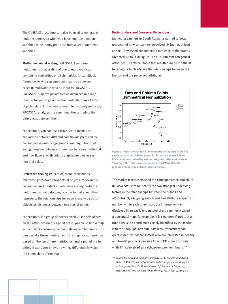
Better Understand Consumer Perceptions
Market researchers in South Australia wanted to better
understand how consumers perceived six brands of iced
coffee. They asked consumers to rate each of the brands
(denoted AA to FF in Figure 1) on 16 different categorical
attributes. The 96-cell table that resulted made it difficult
for analysts to clearly see the relationships between the
brands and the perceived attributes.
The market researchers used the correspondence procedure
in PASW Statistics to identify the two strongest underlying
factors in the relationships between the brands and
attributes. By assigning each brand and attribute a specific
number within each dimension, the information was
displayed in an easily understood chart, commonly called
a perceptual map. For example, it is clear from Figure 1 that
Brand AA is the brand most closely identified by the market
with the “popular” attribute. Similarly, researchers can
quickly identify that consumers who are interested in healthy
and low-fat products perceive CC and DD more positively,
while FF is perceived as a rich, sweet premium brand.**
** Source for data and example: Kennedy, R., C. Riquier, and Byron
Sharp. 1996. “Practical Applications of Correspondence Analysis
to Categorical Data in Market Research,” Journal of Targeting,
Measurement and Analysis for Marketing, Vol. 5, No. 1, pp. 56-70.
The OVERALS procedure can also be used to generalize
multiple regression when you have multiple outcome
variables to be jointly predicted from a set of predictor
variables.
Multidimensional scaling (PROXSCAL) performs
multidimensional scaling of one or more matrices
containing similarities or dissimilarities (proximities).
Alternatively, you can compute distances between
cases in multivariate data as input to PROXSCAL.
PROXSCAL displays proximities as distances in a map
in order for you to gain a spatial understanding of how
objects relate. In the case of multiple proximity matrices,
PROXSCAL analyzes the commonalities and plots the
differences between them.
For example, you can use PROXSCAL to display the
similarities between different cola flavors preferred by
consumers in various age groups. You might find that
young people emphasize differences between traditional
and new flavors, while adults emphasize diet versus
non-diet colas.
Preference scaling (PREFSCAL) visually examines
relationships between two sets of objects, for example,
consumers and products. Preference scaling performs
multidimensional unfolding in order to find a map that
represents the relationships between these two sets of
objects as distances between two sets of points.
For example, if a group of drivers rated 26 models of cars
on ten attributes on a six-point scale, you could find a map
with clusters showing which models are similar, and which
persons like these models best. This map is a compromise
based on the ten different attributes, and a plot of the ten
different attributes shows how they differentially weight
the dimensions of the map.
Figure 1: Researchers studied the consumer perceptions of six iced coffee brands sold in South Australia. Brands are denoted AA to FF and are characterized by various categorical attributes, such as “healthy.” The correspondence procedure in PASW Statistics produced the correspondence map shown here.
FeaturesStatisticsCATREG
■ Categorical regression analysis through
optimal scaling
– Specify the optimal scaling level at which
you want to analyze each variable.
Choose from: Spline ordinal (monotonic),
spline nominal (nonmonotonic), ordinal,
nominal, multiple nominal, or numerical.
– Discretize continuous variables or convert
string variables to numeric integer values
by multiplying, ranking, or grouping values
into a preselected number of categories
according to an optional distribution
(normal or uniform), or by grouping
values in a preselected interval into
categories. The ranking and grouping
options can also be used to recode
categorical data.
– Specify how you want to handle missing
data. Impute missing data with the
variable mode or with an extra category,
or use listwise exclusion.
– Specify objects to be treated as
supplementary
– Specify the method used to compute
the initial solution
– Control the number of iterations
– Specify the convergence criterion
– Plot results, either as:
■ Transformation plots (optimal
category quantifications against
category indicators)
■ Residual plots
– Add transformed variables, predicted
values, and residuals to the working
data file
– Print results, including:
■ Multiple R, R2, and adjusted R2 charts
■ Standardized regression coefficients,
standard errors, zero-order correlation,
part correlation, partial correlation,
Pratt’s relative importance measure
for the transformed predictors, tolerance
before and after transformation, and
F statistics
■ Table of descriptive statistics, including
marginal frequencies, transformation
type, number of missing values,
and mode
■ Iteration history
■ Tables for fit and model parameters:
ANOVA table with degrees of freedom
according to optimal scaling level;
model summary table with adjusted
R2 for optimal scaling, t values, and
significance levels; a separate table
with the zero-order, part and partial
correlation; and the importance and
tolerance before and after transformation
■ Correlations of the transformed
predictors and eigenvalues of the
correlation matrix
■ Correlations of the original predictors
and eigenvalues of the correlation
matrix
■ Category quantifications
– Write discretized and transformed data
to an external data file
■ Three new regularization methods: Ridge
regression, the Lasso, and the Elastic Net
– Improve prediction accuracy by
stabilizing the parameter estimates
– Analyze high-volume data
(more variables than objects)
– Obtain automatic variable selection from
the predictor set
– Write regularized models and coefficients
to a new dataset for later use
■ Two new model selection and predictive
accuracy assessment methods: the .632
bootstrap, and Cross Validation (CV)
– Find the model that is optimal for
prediction with the .632(+) bootstrap
and CV options
– Obtain nonparametric estimates of the
standard errors of the coefficients with
the bootstrap
■ Systematic multiple starts
– Discover the global optimal solution
when monotonic transformations
are involved
– Write signs of regression coefficients to
a new dataset for reuse
CORRESPONDENCE
■ Correspondence analysis
– Input data as a case file or directly as
table input
– Specify the number of dimensions of
the solution
– Choose from two distance measures:
Chi-square distances for correspondence
analysis or Euclidean distances for biplot
analysis types
– Choose from five types of
standardization: Remove row means,
remove column means, remove row-
and-column means, equalize row totals,
or equalize column totals
– Five types of normalization: Symmetrical,
principal, row principal, column
principal, and customized
– Print results, including:
■ Correspondence table
■ Summary table: Singular values,
inertia, proportion of inertia
accounted for by the dimensions,
cumulative proportion of inertia
accounted for by the dimensions,
confidence statistics for the maximum
number of dimensions, row profiles,
and column profiles
■ Overview of row and column points:
Mass, scores, inertia, contribution
of the points to the inertia of the
dimensions, and contribution of the
dimensions to the inertia of the points
■ Row and column confidence statistics:
Standard deviations and correlations
for active row and column points
MULTIPLE CORRESPONDENCE
■ Multiple correspondence analysis (replaces
HOMALS, which was included in versions
prior to SPSS Categories 13.0)
– Specify variable weights
– Discretize continuous variables or
convert string variables to numeric
integer values by multiplying, ranking,
or grouping values into a preselected
number of categories according to an
optional distribution (normal or uniform),
or by grouping values in a preselected
interval into categories. The ranking
and grouping options can also be used
to recode categorical data.
– Specify how you want to handle missing
data. Exclude only the cells of the data
matrix without valid value, impute
missing data with the variable mode or
with an extra category, or use listwise
exclusion.
– Specify objects and variables to be
treated as supplementary (full output is
included for categories that occur only
for supplementary objects)
– Specify the number of dimensions in
the solution
– Specify a file containing the coordinates
of a configuration and fit variables in this
fixed configuration
– Choose from five normalization options:
Variable principal (optimizes associations
between variables), object principal
(optimizes distances between objects),
symmetrical (optimizes relationships
Features subject to change based on final product release. Symbol indicates a new feature.

between objects and variables),
independent, or customized (user-
specified value allowing anything in
between variable principal and object
principal normalization)
– Control the number of iterations
– Specify convergence criterion
– Print results, including:
■ Model summary
■ Iteration statistics and history
■ Descriptive statistics (frequencies,
missing values, and mode)
■ Discrimination measures by variable
and dimension
■ Category quantifications (centroid
coordinates), mass, inertia of the
categories, contribution of the
categories to the inertia of the
dimensions, and contribution of
the dimensions to the inertia of
the categories
■ Correlations of the transformed
variables and the eigenvalues of the
correlation matrix for each dimension
■ Correlations of the original variables
and the eigenvalues of the correlation
matrix
■ Object scores
■ Object contributions: Mass, inertia,
contribution of the objects to the
inertia of the dimensions, and
contribution of the dimensions to
the inertia of the objects
– Plot results, creating:
■ Category plots: Category points,
transformation (optimal category
quantifications against category
indicators), residuals for selected
variables, and joint plot of category
points for a selection of variables
■ Object scores
■ Discrimination measures
■ Biplots of objects and centroids of
selected variables
– Add transformed variables and object
scores to the working data file
– Write discretized data, transformed
data, and object scores to an external
data file
CATPCA
■ Categorical principal components analysis
through optimal scaling
– Specify the optimal scaling level at which
you want to analyze each variable.
Choose from: Spline ordinal (monotonic),
spline nominal (nonmonotonic), ordinal,
nominal, multiple nominal, or numerical.
– Specify variable weights
– Discretize continuous variables or
convert string variables to numeric
integer values by multiplying, ranking,
or grouping values into a preselected
number of categories according to an
optional distribution (normal or uniform),
or by grouping values in a preselected
interval into categories. The ranking
and grouping options can also be used
to recode categorical data.
– Specify how you want to handle
missing data. Exclude only the cells of
the data matrix without valid value,
impute missing data with the variable
mode or with an extra category, or use
listwise exclusion.
– Print results, including:
■ Model summary
■ Iteration statistics and history
■ Descriptive statistics (frequencies,
missing values, and mode)
■ Variance accounted for by variable
and dimension
■ Component loadings
■ Category quantifications and category
coordinates (vector and/or centroid
coordinates) for each dimension
■ Correlations of the transformed
variables and the eigenvalues of
the correlation matrix
■ Correlations of the original variables
and the eigenvalues of the correlation
matrix
■ Object (component) scores
– Plot results, creating:
■ Category plots: Category points,
transformations (optimal category
quantifications against category
indicators), residuals for selected
variables, and joint plot of category
points for a selection of variables
■ Plot of the object (component) scores
■ Plot of component loadings
PROXSCAL
■ Multidimensional scaling analysis
– Read one or more square matrices
of proximities, either symmetrical
or asymmetrical
– Read weights, initial configurations,
fixed coordinates, and independent
variables
– Treat proximities as ordinal (non-metric)
or numeric (metric); ordinal
transformations can treat tied
observations as discrete or continuous
– Specify multidimensional scaling with
three individual differences models, as
well as the identity model
– Specify fixed coordinates or independent
variables to restrict the configuration.
Additionally, specify the transformations
(numerical, nominal, ordinal, and
splines) for independent variables.
PREFSCAL
■ Visually examine relationships between
variables in two sets of objects in order to
find a common quantitative scale
– Read one or more rectangular matrices
of proximities
– Read weights, initial configurations,
and fixed coordinates
– Optionally transform proximities with
linear, ordinal, smooth ordinal, or spline
functions
– Specify multidimensional unfolding
with identity, weighted Euclidean, or
generalized Euclidean models
– Specify fixed row and column
coordinates to restrict the configuration
System requirements ■ Software: PASW Statistics Base* 17.0
■ Other system requirements vary
according to platform
To learn more, please visit www.spss.com. For SPSS office locations and telephone numbers, go to www.spss.com/worldwide.
SPSS is a registered trademark and the other SPSS Inc. products named are trademarks of SPSS Inc. All other names are trademarks of their respective owners. © 2009 SPSS Inc. All rights reserved. SCT1702SPC-0209