path integrals - uni-jena.dep6fusi2/login/skripte/skripte/... · 2009-11-09 · path integrals in...
TRANSCRIPT

Path Integrals
Andreas Wipf
Theoretisch-Physikalisches-Institut
Friedrich-Schiller-Universitat, Max Wien Platz 1
07743 Jena
3. Auflage WS 2008/09
I ask readers to report on errors in the manuscript and hope that the correctionswill bring it closer to a level that students long for but authors find so elusive.
(email to: [email protected]) November 9, 2009

Contents
1 Introduction 4
2 Deriving the Path Integral 82.1 Recall of Quantum Mechanics . . . . . . . . . . . . . . . . . . . . . . . .. . 82.2 Feynman-Kac Formula . . . . . . . . . . . . . . . . . . . . . . . . . . . . . .112.3 Non-stationary systems . . . . . . . . . . . . . . . . . . . . . . . . . . .. . . 142.4 Greensfunctions . . . . . . . . . . . . . . . . . . . . . . . . . . . . . . . . .. 15
3 The Harmonic Oscillator 183.1 Solution by discretization . . . . . . . . . . . . . . . . . . . . . . . .. . . . . 183.2 Oscillator with external source . . . . . . . . . . . . . . . . . . . .. . . . . . 223.3 Mode expansion . . . . . . . . . . . . . . . . . . . . . . . . . . . . . . . . . . 26
4 Perturbation Theory 284.1 Perturbation expansion for the propagator . . . . . . . . . . .. . . . . . . . . 284.2 Quartic potentials . . . . . . . . . . . . . . . . . . . . . . . . . . . . . . .. . 32
5 Particles inE and B fields 345.1 Charged scalar particle . . . . . . . . . . . . . . . . . . . . . . . . . . .. . . 34
5.1.1 The Aharonov-Bohm effect . . . . . . . . . . . . . . . . . . . . . . . 365.2 Spinning particles . . . . . . . . . . . . . . . . . . . . . . . . . . . . . . .. . 38
5.2.1 Spinning particle in constantB-field . . . . . . . . . . . . . . . . . . . 40
6 Euclidean Path Integral 436.1 Quantum Mechanics for Imaginary Times . . . . . . . . . . . . . . .. . . . . 436.2 The Euclidean Path Integral . . . . . . . . . . . . . . . . . . . . . . . .. . . . 466.3 Semiclassical Approximation . . . . . . . . . . . . . . . . . . . . . .. . . . . 47
6.3.1 Saddle point approximation for ordinary integrals . .. . . . . . . . . . 476.3.2 Saddle point approximation in Euclidean Quantum Mechanics . . . . . 50
6.4 Functional Determinants . . . . . . . . . . . . . . . . . . . . . . . . . .. . . 52
1
CONTENTS Contents 2
6.4.1 Calculating determinants . . . . . . . . . . . . . . . . . . . . . . .. . 566.4.2 Generalizing the result of Gelfand and Yaglom . . . . . . .. . . . . . 58
7 Brownian motion 607.1 Diffusion . . . . . . . . . . . . . . . . . . . . . . . . . . . . . . . . . . . . . 607.2 Discrete random walk . . . . . . . . . . . . . . . . . . . . . . . . . . . . . .. 627.3 Scaling limit . . . . . . . . . . . . . . . . . . . . . . . . . . . . . . . . . . . .637.4 Expectation values and correlations . . . . . . . . . . . . . . . .. . . . . . . 657.5 Appendix A: Stochastic Processes . . . . . . . . . . . . . . . . . . .. . . . . 66
8 Statistical Mechanics 728.1 Thermodynamic Partition Function . . . . . . . . . . . . . . . . . .. . . . . . 728.2 Thermal Correlation Functions . . . . . . . . . . . . . . . . . . . . .. . . . . 738.3 Wigner-Kirkwood Expansion . . . . . . . . . . . . . . . . . . . . . . . .. . . 798.4 High Temperature Expansion . . . . . . . . . . . . . . . . . . . . . . . .. . . 818.5 High-T Expansion for/D
2. . . . . . . . . . . . . . . . . . . . . . . . . . . . . 82
8.6 Appendix B: Periodic Greenfunction . . . . . . . . . . . . . . . . .. . . . . . 84
9 Simulations 879.1 Markov Processes and Stochastic Matrices . . . . . . . . . . . .. . . . . . . . 889.2 Detailed Balance, Metropolis Algorithm . . . . . . . . . . . . .. . . . . . . . 92
9.2.1 Three-state system at finite temperature . . . . . . . . . . .. . . . . . 93
10 Berezin Integral 9510.1 Grassmann variables . . . . . . . . . . . . . . . . . . . . . . . . . . . . .. . 95
11 Supersymmetric Quantum Mechanics 101
12 Fermion Fields 10412.1 Dirac fermions . . . . . . . . . . . . . . . . . . . . . . . . . . . . . . . . . .10412.2 The index theorem for the Dirac operator . . . . . . . . . . . . .. . . . . . . 10812.3 The Schwinger model, Part I . . . . . . . . . . . . . . . . . . . . . . . .. . . 110
13 Constrained systems 114
14 Gauge Fields 12014.1 Classical Yang-Mills Theories . . . . . . . . . . . . . . . . . . . .. . . . . . 120
14.1.1 Hamiltonian structure . . . . . . . . . . . . . . . . . . . . . . . . .. . 12114.2 Abelian Gauge Theories . . . . . . . . . . . . . . . . . . . . . . . . . . .. . 12614.3 The Schwinger model, Part II . . . . . . . . . . . . . . . . . . . . . . .. . . . 126
————————————A. Wipf, Path Integrals

CONTENTS Contents 3
15 External field problems 13415.1 The S-matrix . . . . . . . . . . . . . . . . . . . . . . . . . . . . . . . . . . . 13415.2 Scattering in Quantum Mechanics . . . . . . . . . . . . . . . . . . .. . . . . 13515.3 Scattering in Field Theory . . . . . . . . . . . . . . . . . . . . . . . .. . . . 13615.4 Schwinger-Effect . . . . . . . . . . . . . . . . . . . . . . . . . . . . . . .. . 139
16 Effective potentials 14316.1 Legendre transformation . . . . . . . . . . . . . . . . . . . . . . . . .. . . . 14416.2 Effective potentials in field theory . . . . . . . . . . . . . . . .. . . . . . . . 14716.3 Lattice approximation . . . . . . . . . . . . . . . . . . . . . . . . . . .. . . . 15016.4 Mean field approximation . . . . . . . . . . . . . . . . . . . . . . . . . .. . . 154
Index 161
————————————A. Wipf, Path Integrals

Chapter 1
Introduction
These lectures are intended as an introduction to path or functional integration techniques andtheir applications in physics. It is assumed that the participants have a good knowledge inquantum mechanics. No prior exposure to path integrals is assumed, however.
We are all familiar with the standard formulations of quantum mechanics, developed byHEISENBERG, SCHRODINGER and others in the 1920s. In 1933, DIRAC speculated that inquantum mechanic the classical actionS might play a similarly important role as it does inclassical mechanics. He arrived at the conclusion that the amplitude for the propagation fromthe initial positionq′ at time0 to the final positionq at timet,
K(t, q, q′) = 〈q|e−iHt/h|q′〉, (1.1)
is given by
K(t, q, q′) ∼ eiS[wcl]/h, (1.2)
wherewcl is the classical trajectory fromq′ to q in time t. The exponent is dimensionless,since the reduced Planck-constanth has the dimension of an action. For a free particle withHamiltonian and Lagrangian
H0 =1
2mp2 and L0 =
m
2q2 (1.3)
the above formula is easily checked: free particles move on straight lines such that the trajectoryw(s) of a particle moving fromq′ to q and the corresponding action read
w(s) =1
tsq + (t− s)q′ and S =
∫ t
0dt L0(w, w) =
m
2t(q − q′)2. (1.4)
Following Diracs suggestion this leads to the amplitude
K0(t, q, q′) ∼ eim(q−q′)2/2ht. (1.5)
4

CHAPTER 1. INTRODUCTION 5
The factor of proportionality can be inferred from the initial condition
e−iHt/ht→0−→ 1⇐⇒ lim
t→0K(t, q, q′) = δ(q, q′) (1.6)
or alternatively from the convolution property
e−iHt/he−iHs/h = e−iH(t+s)/h
which in position space takes the form∫
duK(t, q, u)K(s, u, q′) = K(t+ s, q, q′). (1.7)
Both ways one arrives at the propagator for a free particle,
K0(t, q, q′) =
( m
2πiht
)1/2eiS[wcl]/h. (1.8)
As we shall see later, similar results hold true for motions in harmonic potentials, for which〈V ′(q)〉 = V ′(〈q〉), such that〈q〉 satisfies the classical equation of motion.
However, for nonlinear systems the formula (1.8) is modified. In 1948 FEYNMAN suc-ceeded in extending Diracs result to interacting systems. He found an alternative formulationof quantum mechanics, based on the fact that the propagator can be written as a sum overallpossible paths(and not just the classical paths) from the initial to the final point. One may saythat in quantum mechanics a particle may move along any pathw(t) connecting the initial withthe final point in timet,
w(0) = q′ and w(t) = q. (1.9)
The amplitude for an individual path is∼ exp (iS[path]/h) and the amplitudes for all paths areadded according to the usual rule for combining probabilityamplitudes,
K(t, q, q′) ∼∑
paths q′→q
eiS[path]/h. (1.10)
Surprisingly enough, the same calculus (in the sense of a analytical continuation) was alreadyknown to mathematicians due to the work of WIENER in the study of stochastic processes. Thiscalculusin functional space attracted the attention of other mathematicians, including KAC, andwas subsequently further developed. The standard reference concerning these achievements isthe review of GELFAND and YAGLOM [5], where the early work was first critically discussed.
The path integral method had its great, early successes in the 1950s and its implicationshave been beautifully expounded in Feynmans original review paper [3] and in his book withHIBBS [4]. This book contains many applications and still serves as a standard literature onpath integrals.
————————————A. Wipf, Path Integrals

CHAPTER 1. INTRODUCTION 6
Path integration provides aunified viewof quantum mechanics, field theory and statisticalphysics and is nowadays a irreplaceable tool in theoreticalphysics. It is an alternative to theHamiltonian method for quantizing classical systems and solving problems in quantum me-chanics and quantum field theories.
These lectures should introduce you both into the formalismand the techniques of pathintegration. We shall discuss applications that will convince you that path integrals are worthstudying not only for reasons of beauty but also for practical purposes.
Path integrals in quantum mechanics and quantum field theoryare ideally suited to deal withproblems like
• Implementing symmetries of a theory
• Incorporating constraints
• Studying non-perturbative effects
• Deriving the semiclassical approximation
• Describing finite-temperature field theories
• Connecting quantum field theories to statistical systems
• Renormalization and renormalization group transformations
• Numerical simulations of field theories.
In the first part of these lecture we shall reformulate ordinary quantum mechanics in Feynmanspath integral language. We shall see how to manipulate path integrals and we shall apply theresults to simple physical systems: theharmonic oscillatorwith constant and time dependentfrequency and the driven oscillator. Then we consider the path integral for imaginary timeand give a precise meaning to the sum over all paths.Functional determinantsshow up inmany path integral manipulations and we devote a whole section to these objects. It follows achapter on the path integral approach to quantum systems in thermal equilibrium. We derive thesemiclassical and high-temperature expansions to the partition functions and conclude the parton quantum mechanics with Monte Carlo simulations of discretized Quantum Mechanics.
In the second part these lectures a simple field-theoreticalmodel, namely the Schwingermodel orQED in 2 dimensions, is introduced and solved. This model is interesting for vari-ous reasons. Due to quantum correction the ’photon’ acquires a mass and the classical chiralsymmetry is broken like it is inQCD. These model allows us to introduce many relevant fieldtheoretical concepts like regularization, Berezin-integrals, gauge fixing and perturbation theory.Then we deal with anomalies and effective actions. We shall see how to employ path integraltechniques to compute anomalies in gauge theories. We ’integrate’ certain anomalies and derive
————————————A. Wipf, Path Integrals
CHAPTER 1. INTRODUCTION 7
the Casimir effect in external fields. Finally we shall compute the particle production in externalelectromagnetic and gravitational fields.
In the last part of these lectures we study the lattice version of field theories. In particularwe introduce and discuss the symmetry breaking by means of effective potentials. Then the nu-merical simulations of scalar theories on a finite lattice isdiscussed. Finally I shall explain howto formulate gauge field theories with fermions on a space-time lattice and the some problemsof these lattice gauge theories.
There are many good books and review articles on path integrals. I have listed some ref-erences which I suggest for further readings. In particularthe references [1]-[9] contain in-troductory material. These references are only a very smalland subjective selection from theextensive literature on functional integrals. In the bibliography at the end of these lectures youfind further references on particular topics of path integrals.
————————————A. Wipf, Path Integrals

Chapter 2
Deriving the Path Integral
Quantization is a procedure for constructing a quantum theory starting from a classical the-ory. There are different approaches to quantizing a classical system, the prominent ones beingcanonical quantizationandpath integral quantization1. In this course I shall assume that youare familiar with the first one, that is the wave mechanics developed by SCHRODINGER and thematrix mechanics due to BORN, HEISENBERGand JORDAN. Here we only recall the importantsteps in a canonical quantization of a classical system.
2.1 Recall of Quantum Mechanics
A classical system is described by its coordinatesqi and momentapi in phase space.Anobservable is identified with a functionO(p, q) on this space. In particular the energyH(p, q)
is an observable. The phase space is equipped with a symplectic structure which means that(locally) it possesses coordinates withPoisson brackets
pi, qj = δ ji , (2.1)
and this structure naturally extends to observables by the derivation ruleOP,Q = OP,Q+
O,QP and the antisymmetry of the brackets. The time-evolution ofany observable is deter-mined by its equation of motion
O = O,H, e.g. qi = qi, H and pi = pi, H. (2.2)
Now one may ’quantize’ a classical system by requiring that observables become hermiteanlinear operators and Poisson brackets are replaced by commutators:
O(p, q) → O(p, q) and O,P −→ 1
ih[O, P ]. (2.3)
1Others would begeometricanddeformation quantization.
8
CHAPTER 2. DERIVING THE PATH INTEGRAL 2.1. Recall of QuantumMechanics 9
In passing we note, that according to a famous theorem of GROENEWOLD [10], later extendedby VAN HOVE [11], there is no invertible linear map from all functionsO(p, q) of phase spaceto hermitean operatorsO in Hilbert space, such that the Poisson-bracket structure is preserved.It is the Moyal bracket, the quantum analog of the Poisson bracket based on the Weyl corre-spondence map, which maps invertible to the quantum commutator.
The evolution of observables which do not explicitly dependon time is determined by theHeisenberg equationof motion
d
dtO =
i
h[H, O] =⇒ O(t) = eitH/hO(0)e−itH/h. (2.4)
In particular the phase-space coordinates become operators and their equations of motion read
d
dtpi =
i
h[H, pi] and
d
dtqi =
i
h[H, qi] with [qi, pj] = ihδij . (2.5)
For example, for a non-relativistic particle with Hamiltonoperator
H = H0 + V , with H0 =1
2m
∑
p2i (2.6)
one finds the familiar equations of motion,
d
dtpi = −V,i and
d
dtqi =
pi2m
. (2.7)
Observables are represented as hermitean linear operatorsacting on a separable Hilbert spaceH (the elements of which define the states of the system)
O(q, q) : H −→ H. (2.8)
Here we do not distinguish between an observable and the corresponding hermitean operator.In the coordinate representation the Hilbert space for a particle on the line is the spaceL2(R)
of square integrable functions onR and and the position- and momentum operators are
(qψ)(q) = qψ(q) and (pψ)(q) =h
i∂qψ(q). (2.9)
In experiments we have access to matrix elements of observables. For example, the expectationvalues of an observable in a given state is given by the diagonal matrix element2 〈ψ|O(t)|ψ〉.The time-dependence of expectation values is determined bythe Heisenberg equation (2.4). Wemay perform at-dependent similarity transformation from theHeisenberg-to theSchrodingerpicture,
Os = e−itH/hO eitH/h and |ψs〉 = e−itH/h|ψ〉. (2.10)
2We drop the hats in what follows.
————————————A. Wipf, Path Integrals

CHAPTER 2. DERIVING THE PATH INTEGRAL 2.1. Recall of QuantumMechanics 10
In particularHs = H. In the Schrodinger picture the observables are time-independent,
Os = e−itH/h(
− i
h[H,O] + O
)
eitH/h = 0. (2.11)
The picture changing transformation (2.10) is a (time-dependent) similarity transformation suchthat matrix elements are invariant,
〈ψ|O(t)|ψ〉 = 〈ψs(t)|Os|ψs(t)〉. (2.12)
The values of observable matrix elements do not depend on thechosen picture. After the picturechanging transformationO(t), |ψ〉 −→ Os, |ψs(t)〉 the states evolve in time according totheSchrodinger equation
ihd
dt|ψs〉 = H|ψs〉. (2.13)
The solution is given by the time evolution (2.10),
|ψs(t)〉 = e−itH/h|ψ〉 = e−itH/h|ψs(0)〉 (H = Hs) (2.14)
and depends linearly on the initial state vector|ψs(0). In the coordinate representation thissolution takes the form
ψs(t, q) ≡ 〈q|ψs(t)〉 =∫
〈q|e−itH/h|q′〉〈q′|ψs(0)〉dq′
=∫
K(t, q, q′)ψs(0, q′)dq′, (2.15)
where we made use of the completeness relation for the position eigenstates,∫
dq′ |q′〉〈q′| = 1 (2.16)
and have introduced the unitarytime evolution kernel
K(t, q, q′) = 〈q|e−itH/h|q′〉. (2.17)
It is theprobability amplitudefor the particle to propagate fromq′ at time0 to q at timet and isoccasionally denoted by
K(t, q, q′) ≡ 〈q, t|q′, 0〉. (2.18)
This evolution kernel (sometimes calledpropagator) will be of great importance when weswitch to the path integral formulation. It satisfies the time dependent Schrodinger equation
ihd
dtK(t, q, q′) = HK(t, q, q′), (2.19)
————————————A. Wipf, Path Integrals

CHAPTER 2. DERIVING THE PATH INTEGRAL 2.2. Feynman-Kac Formula 11
whereH acts on the coordinatesq of the final position. In additionK obeys the initial condition
limt→0
K(t, q, q′) = δ(q − q′). (2.20)
The propagator is uniquely determined by the differential equation and initial condition. For anon-relativistic free particle inRd with HamiltonianH0 as in (2.6) it is a Gaussian function ofthe initial and final coordinatesq′, q ∈ Rd, ,
K0(t, q, q′) = 〈q|e−itH0/h|q′〉 = Adt e
im(q−q′)2/2ht, At =
√m
2πiht. (2.21)
The factor proportional tot−d/2 infront of the exponential function is needed to recover theδ-distribution in the limitt→ 0, see (2.20). In one dimension one has
K0(t, q, q′) = At e
im(q−q′)2/2ht. (2.22)
After this preliminaries we now turn to the path integral representation of the evolution kernel.
2.2 Feynman-Kac Formula
Now we are ready to derive the path integral representation of the evolution kernel in coordinatespace (2.17). The result will be the marvelous formulae of RICHARD FEYNMAN [12] andMARC KAC [13]. The path integral of Feynman is relevant for quantum mechanics and thatof Kac is relevant for statistical physics. The formula of Feynman-Kac is very much related tostochastic differential equations and has many application outside of the realm of physics, forexample in Biology (evolution processes), financing (optimal prizing) or even social sciences(stochastic models of social processes).
In our derivation of the Feynman-Kac formula we shall need theproduct formula of Trotter.In its simplest form, proven by LIE, it states that for two matricesA andB the following formulaholds true
eA+B = limn→∞
(
eA/neB/n)n. (2.23)
To prove this simple formula we introduce then’th roots of the matrices on both sides in (2.23),namelySn := exp[(A+B)/n] andTn := exp[A/n] exp[B/n] and telescope the difference
‖Snn − T nn ‖ = ‖eA+B − (eA/neB/n)n‖= ‖Sn−1
n (Sn − Tn) + Sn−2n (Sn − Tn)Tn + · · ·+ (Sn − Tn)T
n−1n ‖.
Since the matrix-norms of the sum and product of two matricesX andY satisfy‖X + Y ‖ ≤‖X‖ + ‖Y ‖ and‖X · Y ‖ ≤ ‖X‖ · ‖Y ‖ it follows at once that‖ exp(X)‖ ≤ exp(‖X‖) and
‖Sn‖, ‖Tn‖ ≤ e(‖A‖+‖B‖)/n ≡ a1/n.
————————————A. Wipf, Path Integrals
CHAPTER 2. DERIVING THE PATH INTEGRAL 2.2. Feynman-Kac Formula 12
Now we can bound the norm ofSnn − T nn from above,
‖Snn − T nn ‖ ≤ n · a(n−1)/n‖Sn − Tn‖.
Finally, usingSn−Tn = −[A,B]/2n2 +O(1/n3) this proves the product formula for matrices.This theorem and its proof can be extended to the case whereA andB are self-adjoint operatorsand their sumA +B is (essentially) self-adjoint on the intersectionD of the domains ofA andB:
e−it(A+B) = s− limn→∞
(
e−itA/ne−itB/n)n. (2.24)
Moreover, ifA andB are bounded below, then
e−τ(A+B) = s− limn→∞
(
e−τA/ne−τB/n)n. (2.25)
With the strong limit one means that the convergence holds on all states inD. The first for-mulation is relevant for quantum mechanics and the second isneeded in statistical mechanicsand diffusion problems. For a proof of the Trotter product formula for operators I refer to themathematical literature [21, 22].
Using the product formula (2.24) in the evolution kernel (2.17) yields
K(t, q, q′) = limn→∞
〈q| (e−itH0/hne−itV/hn)n|q′〉 . (2.26)
Insertingn − 1-times the resolution of the identity1 =∫
dwj|wj〉 〈wj| associated with theposition eigenstates, we obtain for the matrix element on the right hand side
〈q| e−itH0/hne−itV/hn1 e−itH0/hne−itV/hn1 . . .1 e−itH0/hne−itV/hn|q′〉
=∫
dw1 · · · dwn−1
j=n−1∏
j=0
〈wj+1| e−itH0/hne−itV/hn|wj〉 . (2.27)
In the last formulawn = q is the final position andw0 = q′ the initial position of the particle.Since the potential is diagonal in the coordinate representation we find
〈wj+1| e−itH0/hne−itV/hn|wj〉 = 〈wj+1| e−itH0/hn|wj〉 e−itV (wj)/hn. (2.28)
Now we insert the evolution kernel (2.22) of the free particle and find forKn the representation
K(t, q, q′) = = limn→∞
Anǫ
∫
dw1 · · · dwn−1 · eiS(n)(w)/h
S(n)(w) =m
2
n−1∑
j=0
ǫ(wj+1 − wj
ǫ
)2
−n−1∑
j=0
ǫV (wj) (2.29)
whereǫ = t/n. This is the celebrated formula of Feynman and Kac and it is just thepathintegral representation of the evolution kernel we have been aiming at.
————————————A. Wipf, Path Integrals

CHAPTER 2. DERIVING THE PATH INTEGRAL 2.2. Feynman-Kac Formula 13
b
b
b
b
b
b
b b
bb
0
w0 = q′
ǫ
w1
2ǫ
w2
3ǫ
w3
nǫ
wn = q
Figure 2.1:A broken path of a particle propagating fromw0 town.
To see more clearly why (2.29) is called apath integral(or functional integralin field theory)we divide the time interval[0, t] inton equidistant intervals with lengthǫ = t/n and identifywkwith w(s = kǫ), see fig. (2.1). Now we connect every pair of points(jǫ, wj) and(jǫ+ ǫ, wj+1)
by a straight line and obtain a broken line path fromw0 = q′ town = q
The exponentSL in (2.29) is a Riemann sum approximation to the classical action of aparticle moving along this broken line path,
S(n)(w)n→∞−→
t∫
0
ds(m
2w2 − V (w)
)
≡ S[w] (2.30)
The integrations∫
dw1 . . . dwn−1 in (2.29) is to be interpreted as summing over all possiblebroken line paths connectingq′ with q. Since any continuous path fromq′ with q can be ap-proximated by a broken line path and since finally we must takethe continuum limitn→ ∞ orequivalentlyǫ → 0, we may interpret the integral (2.29) as a sum over all paths from q′ at time0 and toq at timet. Theǫ-dependent constant
Anǫ =(
m
2πihǫ
)n/2
(2.31)
in the path integral (2.29) is required to obtain a unitary time evolution. It diverges in thecontinuum limitǫ → 0, but this divergence is harmless as we shall see later. In thecontinuumlimit we denote the path integral representation for the evolution kernel (2.29) by
K(t, q, q′) =
w(t)=q∫
w(0)=q′
Dw eiS[w]/h, (2.32)
with the formal ’measure’Dw on the set of paths defined by the limit (2.29). Since the infiniteproduct of Lebesgue measures like
∏∞1 dwj fails to be a measure, the symbolDw is mathemati-
cally not well-defined. However, one can define a measure on the set of paths if one analytically
————————————A. Wipf, Path Integrals

CHAPTER 2. DERIVING THE PATH INTEGRAL 2.3. Non-stationary systems 14
continues to imaginary time. For more general Lagrangian systems, for example for particlespropagating in3 dimensions, a similar path integral representation for theevolution kernel canbe given. In same cases, for example for particle in externalfields, ordering ambiguities in thecanonical approach translate into discretization ambiguities even in the continuum limit.
2.3 Non-stationary systems
The Feynman-Kac formula not only holds for stationary systems, it also holds for time-dependentHamiltoniansH(t) for which the evolution kernel has the form
K(t, q, t′, q′) = 〈q|T exp(
− i
h
∫ t
t′H(s)ds
)
|q′〉 , (2.33)
whereT denotes the time ordering. The generalization to time-dependent Hamiltonians is usefulwhen on considers system under varying external conditions, for example in a time-dependentexternal field. In a non-stationary situation the evolutionoperator depends on the initial andfinal times and not only on the time-differencet − t′. But the continuum path integral for theevolution kernelK looks the same as in the stationary case,
K(t, q, t′, q′) =
w(t)=q∫
w(t′)=q′
Dw eiS[w]/h, (2.34)
where now the Lagrange function depends explicitly on time.For a system with HamiltonianH = H0 + V (t) the path integral is the continuum limit of
K(t, q, t′, q′) = limn→∞
Anǫ
∫
dw1 · · · dwn−1 eiS(n)(w)/h
S(n)(w) =m
2
n−1∑
j=0
(wj+1 − wj
ǫ
)2
−n−1∑
j=0
ǫV (t′ + jǫ, wj), (2.35)
whereǫ = (t−t′)/n. Note that now the potential depends on the (discretized) time. To establish(2.34) we show that
ψ(t, q) =∫
K(t, q, t′, q′)ψ(t′, q′) dq′ (2.36)
obeys the time-dependent Schrodinger equation. For that purpose we sett′ = t − ǫ with smallǫ. The evolution for a infinitesimal time stepǫ is given by
ψ(t, q) = Aǫ
∫
dq′ expim
2hǫ(q − q′)2 − iǫ
hV (t− ǫ, q′)
ψ(t− ǫ, q′).
Changing variables according toq → q′ + u this reads
ψ(t, q) = Aǫ
∫
du eimu2/2hǫe−iǫV (t−ǫ,q+u)/h ψ(t− ǫ, q + u). (2.37)
————————————A. Wipf, Path Integrals

CHAPTER 2. DERIVING THE PATH INTEGRAL 2.4. Greensfunctions15
Due to the first Gaussian factor theu-integral gets its main contribution from the neighborhoodof u = 0 and thus we may expand the last two factors in powers ofu. The resulting integralsoveru are computed with the help of the formula
∫
du u2neimu2/2hǫ =
1
Aǫ
(
ihǫ
m
)n
(2n− 1)!! (2.38)
where0!! = (−1)!! = 1 by definition. Of course, the integrals with odd powers ofu vanish. Weonly need the terms of order1 andǫ on the right hand side in (2.37) and thus it is sufficient toexpandψ to second order inu. Up to terms of orderǫ2 we find
ψ(t, q) = Aǫ
∫
du eimu2/2hǫ
(
1 − iǫ
hV (t, q)
)(
ψ(t− ǫ, q) +u2
2ψ′′(t, q)
)
+O(ǫ2).
The integration overu finally leads to
ψ(t, q) = ψ(t− ǫ, q) − iǫ
hV (t, q)ψ(t, q) +
ihǫ
mψ′′(t, q) +O(ǫ2). (2.39)
Note that forǫ→ 0 the right hand side converges toψ(t, q) such thatK converges to the identityast′ → t. Now we subtractψ(t−ǫ, q) from both sides in (2.39) and divide the resulting equationby ǫ. In the continuum limitǫ→ 0 we recover the time-dependent Schrodinger equation,
ih∂ψ
∂t= − h2
2mψ′′ + V (t)ψ, (2.40)
and this shows that even for a time-dependent Hamiltonian the propagator is given by the pathintegral (2.34) or more accurately by (2.35).
2.4 Greensfunctions
In quantum field theory one is interested in vacuum expectation values of time-ordered productsof Heisenberg field operators since these objects are related to amplitudes of physical processessuch as scattering amplitudes or decay rates of particles. We look at the analogous objects inquantum mechanics:
G(n)(t1, t2, . . . , tn) = 〈Ω|T q(t1)q(t2) · · · q(tn)|Ω〉, (2.41)
where|Ω〉 represents the vacuum state and the position operator has the time dependence
q(t) = eitH/hqe−itH/h, (2.42)
see equation (2.4). The objectsG(n) are known asGreensfunctionor correlation functions. Thetime ordering operatorT orders its arguments such that the operator at earliest timeacts first (isthe right-most), the operator at the second earliest time acts next etc. For example
T q(t1)q(t2) =
q(t1)q(t2) t1 > t2q(t2)q(t1) t2 > t1.
(2.43)
————————————A. Wipf, Path Integrals

CHAPTER 2. DERIVING THE PATH INTEGRAL 2.4. Greensfunctions16
Now will derive the path integral expression for the Greensfunction (2.41). Actually we shallcalculate correlation functions with fixed endpoints, for example
〈q, t|T q(t1)q(t2)|q′〉 , where |q, t〉 = eitH/h|q〉 (2.44)
is the past-evolved position eigenstate,q(t)|t, q〉 = q|t, q〉. Later we shall see how one recoversthe vacuum expectation values (2.41) from the correlation functions with fixed endpoints. Weassumet1 > t2 and insert twice the identity in (2.44), one after every position operatorq,
〈q, t| q(t1)q(t2)|q′〉 = 〈q| e−i(t−t1)H qe−i(t1−t2)H qe−it2H |q′〉=∫
dw1dw2 〈q| e−i(t−t1)H |w1〉w1 〈w1| e−i(t1−t2)H |w2〉w2 〈w2| e−it2H |q′〉 .
Inserting the path integral representation for the three matrix elements we obtain
〈q, t| q(t1)q(t2)|q′〉 =∫
dw1dw2w1w2
w(t)=q∫
q(t1)=w1
Dw eiS/hw(t1)=w1∫
w(t2)=w2
Dw eiS/hw(t2)=w2∫
q(0)=q′
Dw eiS/h. (2.45)
This expression consists of a first path integral from the initial positionq′ to the positionw2, asecond one fromw2 to the positionw1, and a third one fromw1 to the final positionq. So weare integrating over all paths fromq′ to q, subject to the restriction that the paths pass throughthe intermediate pointsw2 andw1 at timest2 andt1, respectively. Finally we integrate over thetwo arbitrary positionsw2 andw1, so that in fact we are integrating overall paths. Thus we maycombine the three path integrals and the integrations overw1 andw2 into a single path integral.The factorsw1 andw2 in the integrand are just the valuesw(t1) andw(t2) of the paths at theintermediate times. Hence we end up with
〈q, t| q(t1)q(t2)|q′〉 =
w(t)=q∫
w(0)=q′
Dww(t1)w(t2) eiS[w]/h (t1 > t2). (2.46)
A similar calculation reveals that the same result holds true for the matrix element ofq(t2)q(t1)whent2 > t1. The path integral takes care of the time ordering. Thus we arrive at the followingformula for all pairst1, t2:
〈q, t|T q(t1)q(t2)|q′〉 =
w(t)=q∫
w(0)=q′
Dww(t1)w(t2) eiS[w]/h. (2.47)
The generalization to higher correlation function is evident. One obtains
〈q, t|T q(t1)q(t2) · · · q(tn)|q′〉 =
w(t)=q∫
w(0)=q′
Dww(t1)w(t2) · · ·w(tn) eiS[w]/h. (2.48)
————————————A. Wipf, Path Integrals

CHAPTER 2. DERIVING THE PATH INTEGRAL 2.4. Greensfunctions17
Now we relate the time ordered correlation functions for fixed endpoints to the vacuum expecta-tion values in (2.41). Normalizing the Hamiltonian such that its groundstate|Ω〉 has zero energy,in which case it is time-independent, we obtain
〈Ω| =∫
dq 〈Ω| q, t〉 〈t, q| =∫
dq 〈Ω| q〉 〈t, q| =∫
dq Ω(q) 〈t, q| . (2.49)
Now we multiply (2.48) withΩ(q)Ω(q′) and integrate over the argumentsq andq′. This yields
〈Ω|T q(t1) · · · q(t1)|Ω〉 =∫
dqdq′ Ω(q)Ω(q′)
w(t)=q∫
w(0)=q′
Dww(t1) · · ·w(tn) eiS[w]/h. (2.50)
Actually, to calculate such vacuum-to-vacuum transition amplitudes one conveniently continuesto imaginary time and this will be studied in a later chapter.
Generating functional for time ordered products: The Greenfunctions for time orderedproducts of position operators at different times are generated by a functional depending on anexternal source. It is given by the path integral in which a source term is added to the action,
S[w] −→ Sj [w] = S[w] + (j, w), (j, w) =∫ t
0dsj(s)w(s). (2.51)
The corresponding evolution kernel in the presence of the source
K(t, q, q′; j) =
w(t)=q∫
w(0)=q′
Dw eiSj [w]/h. (2.52)
is just thegenerating functionalfor the Greenfunctions (2.48). For example, its first variationalderivative with respect to the source is
h
i
δ
δj(t1)K(t, q, q′; j) =
∫
Dww(t1) eiSj/h. (2.53)
Then-fold differentiation ofK at j = 0 yields the path integral with severalw-insertions,
h
i
δ
δj(t1)· · · h
i
δ
δj(tn)K(t, q, q′; j)|j=0 =
∫
Dww(t1) · · ·w(tn) eiS[w]/h, (2.54)
which according to the result (2.48) is equal to the expectation value of the time-ordered productof n position operators at different times
h
i
δ
δj(t1)· · · h
i
δ
δj(tn)K(t, q, q′; j)|j=0 = 〈q, t|T q(t1) · · · q(tn)|q′〉 . (2.55)
For an interacting system the generating functional cannotbe calculated in closed form. Butwith the result (2.48) we can easily set up a perturbative expansion for the Greenfunctions. Thiswill be done in chapter 4.
————————————A. Wipf, Path Integrals

Chapter 3
The Harmonic Oscillator
To get acquainted with path integrals we consider the harmonic oscillator for which the pathintegral can be calculated in closed form. We allow for an arbitrary time-dependent oscillatorstrength and later include a time dependent external force.We begin with the discretized pathintegral (2.29) and then turn to the continuum path integral(2.32).
3.1 Solution by discretization
The action of a one-dimensional harmonic oscillator with massm is
S =m
2
∫ t
t′ds(
w2(s) − ω2(s)w2(s))
, (3.1)
whereω(s) is atime-dependentcircular frequency. To calculate the propagator fromq′ at initialtimet′ to q at final timetwe divide the time interval inn intervals of equal lengthǫ = (t−t′)/n.Our starting point is (2.35) with the following classical action for a broken line path
S(n)(w) =m
2
n−1∑
j=0
[1
ǫ(wj+1 − wj)
2 − ǫ ω2jw
2j
]
with ωj = ω(t′ + jǫ). (3.2)
For the following manipulations is it convenient to introduce twon − 1-tupels, one with theintegration variables as entries and the other with the positions of the endpoints,
ξ = (w1, w2, . . . , wn−1) and η = (q′, 0, . . . , 0︸ ︷︷ ︸
n−3 times
, q). (3.3)
Then the action can be rewritten as
S(n)(w) = S(n)(η, ξ) =m
2
(1
ǫ(η, η) +
1
ǫ(ξ, Cξ)− 2
ǫ(ξ, η) − ǫ ω2
0q′ 2)
, (3.4)
18

CHAPTER 3. THE HARMONIC OSCILLATOR 3.1. Solution by discretization 19
where then− 1-dimensional matrixC is
C =
µ1 −1 0 · · · 0
−1 µ2 −1 · · · 0...
...0 −1 µn−1
, µj = 2 − ǫ2ω2j . (3.5)
For vanishingωj the square matrixC is proportional to the discretized second derivative (one-dimensional lattice Laplacian) on the discrete time lattice. We are left with calculating theGaussian integral
Kω(t, q, t′, q′) = lim
n→∞Anǫ
∫
dn−1ξ eiS(n)(ξ,η)/h, where Aǫ =
(m
2πihǫ
)1/2
, (3.6)
and the lattice action (3.4) is a quadratic function of the integration variablesξ. As a functionof these variables it is extremal atξcl, given by
δS(n)
δξi(ξ = ξcl) = 0 or Cξcl = η. (3.7)
ξcl is the classical solution of the discretized equation of motion. Expanding the action aboutthis solution yields
S(n)(ξcl + ξ) = S(n)(ξcl) +m
2ǫ(ξ, Cξ) (3.8)
with the following action of the classical solution
S(n)(ξcl) =m
2ǫ
[
η2 − (η, C−1η)]
− 1
2mω2
0ǫq′2. (3.9)
Terms linear inξ are absent sinceξcl is an extremum ofS. Inserting (3.9) into (3.6) leads to
Kω(t, q, t′, q′) = lim
n→∞Anǫ e
iS(n)(ξcl)/h∫
dn−1ξ e im/2ǫh (ξ,Cξ). (3.10)
Here we encounter for the first time aGaussian integral. Such integrals appear frequently inpath integral calculations. The one-dimensional Gaussianintegral is
∫
dξ e−αξ2/2 =
√
2π
α. (3.11)
The generalization to multi-dimensional Gaussian integrals follows after a diagonalization ofthe matrix defining the quadratic form in the exponent and is given by
∫
d pξ exp(
−1
2(ξ, Bξ)
)
=(2π)p/2√
detB. (3.12)
————————————A. Wipf, Path Integrals

CHAPTER 3. THE HARMONIC OSCILLATOR 3.1. Solution by discretization 20
HereB is ap-dimensional symmetric matrix with non-negative real part. For a non-symmetricB the antisymmetric part does not contribute to the integral andB is replaced by(B + B†)/2
on the right hand side. For an imaginaryB the result (3.12) holds in the distributional sense.Using this useful formula in (3.10) and performing the continuum limit yields
Kω(t, q, t′, q′) = lim
ǫ→0
√m
2πih
1√ǫ detC
eiS(n)(ξcl)/h. (3.13)
It remains to calculate the determinant of the matrixC and the matrix element(η, C−1η) enter-ing the classical action in (3.9).
To find the determinant of then− 1-dimensional matrixC in (3.6) we consider thep-dimensional matrix
Cp =
µ1 −1 0 · · · 0
−1 µ2 −1 · · · 0...
......
0 · · · −1 µp
, µj = 2 − ǫ2ω2j , (3.14)
and denote its determinant bydp. Expanding the determinant in the last row yields the recursionrelationdp = µpdp−1−dp−2 with the initial conditionsd1 = µ1 andd0 = 1. To solve thisrecursion relation we write it in the form
dp − 2dp−1 + dp−1 = −ǫ2ωpdp−1 (3.15)
and divide byǫ2. Furthermore we setdp = d(sp), wheresp = t′ + pǫ denotes the time afterptime-steps have passed since the initial timet′. For ǫ → 0 we may approximate differences bydifferentials such that the recursion relation turns into the differential equation,
d(s) = −ω2(s)d(s). (3.16)
The initial slope ofd diverges in the continuum limit sinced2 − d1 = 1 + O(ǫ2). Hence werescaled(s) → D(s) = ǫ d(s) in order to get a non-singular function. At initial timet′ therescaled function vanishes and has unit slope. Hence in the continuum limit we have
ǫ detC = ǫdn−1ǫ→0−→ D(t, t′), (3.17)
where theD-function solves theGelfand-Yaglom initial value problem[5]
d2D(s, t′)
ds2= −ω2(s)D(t, t′), D(t′, t′) = 0,
∂D(s, t′)
∂s|s=t′ = 1. (3.18)
Note that the D-function depends on the initial timet′ since it solves the initial values problem.The determinant is the values ofD at the final timet. The factorǫ in ǫ detC = D(t) chancelsagainstǫ in (3.15) and in the continuum limit we obtain a finite evolution kernel.
————————————A. Wipf, Path Integrals
CHAPTER 3. THE HARMONIC OSCILLATOR 3.1. Solution by discretization 21
Besides the determinant we need the matrix element(η, C−1η) in the classical action. Itonly depends on the elements in the corners of the matrixC−1. These are given by
C−1 =1
dn−1
cn−2 · · · 1
. · · · .
1 · · · dn−2
, (3.19)
The elements on the diagonal arecn−2 = d(t, t′ + ǫ) anddn−2 = d(t − ǫ, t′). Expanding inǫthe classical action is now seen to depend only on the functionD and its time derivatives as theinitial and final time as follows,
S(n)(wcl)ǫ→0−→ S[wcl] =
m
2D(t, t′)
(
q2 dD(t, t′)
dt− q′ 2
dD(t, t′)
dt′− 2qq′
)
. (3.20)
Since the solutionD of the initial value problem (3.18) determines both the classical action andthe determinantal factor, see (3.17), it determines the exact time evolution kernel
Kω(t, q, t′, q′) =
√m
2πhi
1√
D(t, t′)eiS[wcl]/h. (3.21)
Differentiating the action of the classical pathS[wcl] with respect to the initial and final positionwe recover theD-function,
1
m∂q∂q′S[wcl] = − 1
D(t, t′). (3.22)
We see that the classical action determines both the phase factor and the determinantel factorinfront of the phase factor. The evolution kernel of the time-dependent oscillator is completelydetermined by the classical action,
Kω(t, q, t′, q′) =
√
1
2πhi
(
−∂2S[wcl]
∂q∂q′
)1/2
e iS[wcl]/h. (3.23)
For the oscillator withconstant frequencyω theD-function reads
D(t, t′) =1
ωsinω(t− t′). (3.24)
Settingt′ = 0 we find the following explicit formula for the evolution kernel
Kω(t, q, q′) =
√
mω
2πih sin(ωt)exp
imω
2h
[
(q′2+ q2) cot(ωt) − 2qq′
sin(ωt)
]
. (3.25)
It is not difficult to see that this kernel satisfies the Schrodinger equation and fort → 0 itreduces to the free evolution kernel (2.22) and thus to the delta function. Hence it obeys the
————————————A. Wipf, Path Integrals

CHAPTER 3. THE HARMONIC OSCILLATOR 3.2. Oscillator with external source 22
initial condition (2.20). The kernelKω(t, q, q′) is singular forωt = nπ. This apparent problem
can be dealt with by integrating the kernel against wave packets. The Feynman path integral for
ψ(t, q) =∫
dq′ 〈q|e−itH/h|q′〉ψ0(0, q′), (3.26)
has no singularities.After this rather involved manipulation let us recapitulate the crucial steps in deriving the
evolution kernels. First we replaced the integration variablesξ by ξcl + ξ, whereξcl has beenan extremum of the classical ’action’. This shift eliminates the linear inξ terms in the clas-sical action. Without mentioning, we also assumed the measure to be translational invariant,dn−1(ξcl + ξ) = dn−1ξ, which is of course correct for a finite product of Lebesgue measures.The resulting Gaussian integral can be calculated and is given in (3.13).
3.2 Oscillator with external source
One may wonder whether theformal continuum path integralis of any practical use for realisticquantum systems. Fortunately the answer is yes and we shall see how to use the continuum pathintegral if one allows for certain formal manipulations.
Here we derive the path integral for an oscillator with time-dependent frequency and drivenby a time-dependent and position-independentexternal force. The Hamiltonian function reads
H =1
2mp2 +
m
2ω2q2 − jq, (3.27)
where the time-dependent sourcej(s) is proportional to the external force. The classical actionentering the continuum path integral (2.32) reads
Sj[w] = S[w] + (j, w), where (j, w) =∫ t
t′ds j(s)w(s) (3.28)
andS denotes the action (3.1) of the oscillator without externalforce. By considering the forcedoscillator we shall encounter several problems which one comes across in various approxima-tions to more realistic and complicated systems. In addition, the resulting path integral yieldsthe generating functional for the Greenfunctions and thus will be of use when we derive theperturbation expansion for interacting quantum system.
Classical solutions are extremal points of the action and fulfill the equation of motion
−δS[w]
δw(s)
∣∣∣wcl
= mwcl(s) +mω2(s)wcl(s) = j(s). (3.29)
Similarly as for the discrete path integral considered in the previous section we expand anarbitrary path about the classical trajectory,
w(s) −→ wcl(s) + ξ(s), where wcl(t′) = q′ and wcl(t) = q. (3.30)
————————————A. Wipf, Path Integrals
CHAPTER 3. THE HARMONIC OSCILLATOR 3.2. Oscillator with external source 23
The classical pathwcl obeys the boundary conditions such that the fluctuationsξ vanishes at theendpoints,ξ(t′) = ξ(t) = 0. With
Sj [wcl + ξ] = Sj[wcl] + S[ξ], (3.31)
the path integral for the propagator reads
Kω(t, q, t′, q′; j) =
∫
Dw eiSj [w]/h = eiSj [wcl]/h
ξ(t)=0∫
ξ(t′)=0
Dξ eiS[ξ]/h. (3.32)
The path integral factorizes into a classical part depending on the source and the endpointsand a path integral over the fluctuations. The latter is just the propagatorKω of the force-freeoscillator (3.21) for the propagation fromq′ = 0 to q = 0. For vanishing endpoints the actionS[wcl] enteringKω in (3.21) is zero and we obtain the simple formula
Kω(t, q, t′, q′; j) =
√m
2πhi
1√
D(t, t′)eiSj [wcl]/h, (3.33)
where theD-function solves the initial value problem (3.18).Let us finally isolate the part of the classical action depending on the sourcej. To that aim
we decompose the classical pathwcl into the classical pathw0cl starting and ending at the origin
and the solutionwh of the homogeneous equation of motion (without source) starting atq′ andending atq,
wcl(s) = w0cl(s) + wh(s),
δS
δw
∣∣∣w0
cl
= −j, w0cl(t
′) = 0, w0cl(t) = 0
δS
δw
∣∣∣wh
= 0, wh(t′) = q′, wh(t) = q. (3.34)
Without external source an oscillator at the origin stays atthe origin such thatw0cl(s) = 0 for a
vanishing source. On the other hand , forq′ = q = 0 the homogeneous solutionwh(s) vanishes.The action ofwcl decomposes as
Sj[wcl] = Sj [w0cl] + Sj [wh] +m
∫
w0clwh −m
∫
ω2w0clwh.
After a partial integration in the integral ofwhw0cl the last two term can be written as
m∫ t
t′
d
ds(w0
clwh) −m∫ t
t′w0
cl(wh + ω2wh) = 0.
The first term is zero becausew0cl vanishes at the endpoints and the second term is zero because
wh obeys the homogeneous equation of motion. Thus we obtain
Sj [wcl] = Sj[w0cl] + S[wh] +
∫
ds j(s)wh(s). (3.35)
————————————A. Wipf, Path Integrals
CHAPTER 3. THE HARMONIC OSCILLATOR 3.2. Oscillator with external source 24
When the source is switches off then the action reduces to thesource-independent termS[wh]
and the propagator reduces to the kernelKω in (3.21), such that
Kω(t, q, t′, q′; j) = Kω(t, q, t
′, q′) eiWω[j]/h, (3.36)
where we introduced theSchwinger functionalfor the harmonic oscillator
Wω[j] =∫
ds j(s)wh(s) + Sj [w0cl]
=∫
dsj(s)wh(s) +1
2
∫
dsj(s)w0cl(s). (3.37)
To prove the last identity one uses the equation of motion forthe classical pathw0cl. In order to
find the explicit source dependence of the Schwinger functional we introduce the Greensfunc-tionGD with respect toDirichlet boundary conditions,
m
(
d
ds2+ ω2(s)
)
GD(s, s′) = δ(s, s′). (3.38)
As Greenfunction of a selfadjoint and real operatorGD is symmetric in its arguments and van-ishes at the endpoints,
GD(s, s′) = GD(s′, s) and GD(t, s) = GD(s, t′) = 0. (3.39)
Now we can construct the solutionw0cl with the help of this Greensfunction as follows,
w0cl(s) =
∫ t
t′GD(s, s′)j(s′)ds′. (3.40)
Inserting this result into (3.37) yields the following expression for the Schwinger functional,
Wω[j] =∫
ds j(s)wh(s) +1
2
∫
dsds′ j(s)GD(s, s′)j(s′). (3.41)
The first term is linear and the second is quadratic in the source. Note that according to (2.55)and (2.52) the kernel in (3.36) generates all Greenfunctions of time-ordered products of the po-sition operators at different times. For example, the correlator of two positions for the oscillatorwithout source is
〈q, t|T q(t1)q(t2)|q′〉 =
(
δWω
δj(t1)
δWω
δj(t2)+h
i
δ2Wω
δj(t1)δj(t2)
)∣∣∣j=0
Kω(t, q, t′, q′)
=
(
wh(t1)wh(t2) +h
iGD(t1, t2)
)
Kω(t, q, t′, q′). (3.42)
Next we calculate the kernel and in particular the Schwingerfunctional for the free particle andfor the oscillator with constant frequency.
————————————A. Wipf, Path Integrals
CHAPTER 3. THE HARMONIC OSCILLATOR 3.2. Oscillator with external source 25
Free particle
For simplicity we taket′ = 0 as initial propagation time of the free particle. The Greenfunctionand homogeneous solution are
GD(s > s′) =1
mt(s− t)s′ and wh(s) =
1
t[sq + (t− s)q′]. (3.43)
The quadratic Schwinger functional (3.41) for the free particle has the explicit form
W0[j] =1
t
∫ t
0ds (sq + (t− s)q′)j(s) +
1
mt
∫ t
0ds∫ s
0ds′ (s− t)s′j(s)j(s′) (3.44)
and it enters the propagator in the presence of an external source
K0(t, q, q′; j) = K0(t, q, q
′) eiW0[j]/h. (3.45)
Note that for vanishing endpoints we arrive at the simpler formula
K0(t, 0, 0; j) =(
m
2πiht
)1/2
exp
i
h
∫ t
0ds∫ s
0ds′
(s− t)s′
mtj(s)j(s′)
. (3.46)
Harmonic oscillator with constant frequency
Again we take as initial timet′ = 0. For a constant frequencyω the Greenfunction and solutionof the source-free oscillator read
GD(s > s′) =1
mω sinωtsinω(s− t) sinωs′
wh(s) =1
sinωtq sinωs+ q′ sinω(t− s). (3.47)
Hence the Schwinger function of the oscillator has the explicit form
Wω[j] =1
ω sinωt
∫ t
0ds (q sinωs+ q′ sinω(t− s)q)j(s)
+1
mω sinωt
∫ t
0ds∫ s
0ds′ sinω(s− t) sinωs′ j(s)j(s′), (3.48)
and for a vanishing frequency is converges to the Schwinger functional of the free particle. ThefunctionalWω enters the formula for the propagator of the oscillator withconstant frequency
Kω(t, q, q′; j) = Kω(t, q, q
′) eiWω [j]/h. (3.49)
For vanishing endpoints the evolution kernel forj = 0 on the right hand side simplifies furtherand we obtain the simple formula
Kω(t, 0, 0; j) =
√mω
2πih sinωtexp
i
h
∫ t
0ds∫ s
0ds′
sinω(s− t) sinωs′
mω sinωtj(s)j(s′)
. (3.50)
It generates all correlations of time-ordered products of oscillator positions at different times.
————————————A. Wipf, Path Integrals
CHAPTER 3. THE HARMONIC OSCILLATOR 3.3. Mode expansion26
3.3 Mode expansion
The path integral (3.32) factorizes into a factor containing the action of the classical trajectorywcl with prescribed initial and final positions and a factor containing the path integral over thefluctuationsξ. The latter is independent of the endpoints since the fluctuations vanish fort′ andt and for its computation we need the explicit form of the action
S[ξ] =1
2(ξ, S ′′ξ) with S ′′ = −m
(
d2
ds2+ ω2(s)
)
. (3.51)
The operatorS ′′ is calledfluctuation operatorsince it acts on the fluctuations aboutwcl. It is aself-adjoint operator on functions vanishing at timest′ andt. Hence we can diagonalize it
S ′′ξn = λnξn, where ξn(t′) = ξn(t) = 0. (3.52)
The eigenmodes may be chosen to be orthonormal
(ξn, ξm) ≡∫ t
t′ds ξn(s)ξm(s) = δn,m, (3.53)
and an arbitrary fluctuationξ(s) can be expanded in terms of these modes,
ξ(s) =∑
n
anξn(s). (3.54)
Since the mapξ(s) −→ an is aunitary mapformL2 to ℓ2 the ’measure’ inDξ is equal to the’measure’
∏dan. Inserting the expansion into the exponent in (3.32) we obtain
ξ(t)=0∫
ξ(t′)=0
Dξ ei(ξ,S′′ξ)/2h =∫∏
dan eiλna2n/2h =
∏(
2πih
λn
)1/2
. (3.55)
The product of the eigenvaluesλn is the determinant of the fluctuation operatorS ′′ and thus thepath integral leads to an inverse square root of the determinant ofS ′′,
Kω(t, q, t′, q′) =
N√
det(∂2 + ω2)eiS[wcl]/h. (3.56)
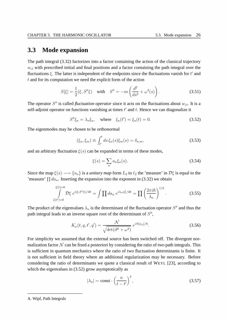
For simplicity we assumed that the external source has been switched off. The divergent nor-malization factorN can be fixed a posteriori by considering the ratio of two path integrals. Thisis sufficient in quantum mechanics where the ratio of two fluctuation determinants is finite. Itis not sufficient in field theory where an additional regularization may be necessary. Beforeconsidering the ratio of determinants we quote a classical result of WEYL [23], according towhich the eigenvalues in (3.52) grow asymptotically as
|λn| ∼ const·(
n
t− t′
)2
, (3.57)
————————————A. Wipf, Path Integrals

CHAPTER 3. THE HARMONIC OSCILLATOR 3.3. Mode expansion27
implying that the determinant does not exist. This is not surprising since already in the regular-ized path integral on the time lattice (3.17)detC ∼ 1/ǫ also tends to infinity in the continuumlimit. The problem with this harmless divergence is resolved as follows: imagine that we repeatthe same steps leading to (3.56) for the free particle instead of the oscillator. We obtain
K0(t, 0, t′, 0) =
N√
det(∂2), (3.58)
since the classical trajectory starting and ending at the origin is justwcl(s) = 0 and hence theactionS[wcl] in (3.56) vanishes in this case. On the other hand we know from(2.21) that
K0(t, 0, t′, 0) =
√
m
2πih(t− t′). (3.59)
Now we divide the evolution kernel in (3.56) byK0 as in (3.58) and multiply again byK0 as in(3.59). The unknown constantN chancels in the quotient and we obtain
Kω(t, q, t′, q′) =
√
m
2πih(t− t′)
(
det∂2 + ω2(.)
∂2
)−1/2
eiS[wcl]/h. (3.60)
According to (3.17) the ratios of the determinants are givenby the ratios of theD-functions ofthe corresponding fluctuation operators. TheD-function of∂2 isD(s, t′) = s− t′, such that
Kω(t, q, t′, q′) =
√m
2πih
1√
D(t, t′)eiS[wcl]/h. (3.61)
Alternatively we could divide and multiply (3.56) with the evolution kernelKω of the oscillatorwith constantω, as given in (3.25). One finds
Kω(t, q, t′, q′) =
√
mω
2πih sinω(t− t′)
(
det∂2 + ω2(.)
∂2 + ω2
)−1/2
eiS[wcl]/h, (3.62)
whereω andω(.) are the constant and time-dependent frequencies. Inserting theD-function1/ω · sinω(t− t′) of the oscillator with constant frequency again leads to theresult (3.61).
————————————A. Wipf, Path Integrals
Chapter 4
Perturbation Theory
In conventional perturbation theory one assumes that the coupling constantλ in
H = H0 + λV (4.1)
is small and expands the eigenvalues and eigenfunctions ofH in a power series inλ. Here weperform an expansion of the evolution kernel in powers of thecoupling constant. ForH0 oneusually takes the Hamiltonian of the free particle or the harmonic oscillator such that forλ = 0
the problem is soluble. This way one obtains a non-convergent series which (at least in quantummechanics) has a good chance of being asymptotic.
4.1 Perturbation expansion for the propagator
We consider a particle with massm in a given external potentialV . We decompose the actioninto a termS0 belonging to the free particle with massm and a termSI describing the interactionof the particle with the potential,
S = S0 + SI =m
2
∫ t
0w 2ds− λ
∫ t
0V (w(s))ds. (4.2)
The coupling constantλ measures the strength of the interaction. It is introduced for an easyidentification of terms contributing to a given order in the perturbative expansion. In order tofind this expansion for the propagator we use its path integral representation
K(t, q, q′) =
w(t)=q∫
w(0)=q′
Dw eiS[w]/h, (4.3)
where one integrates over all paths with fixed endpointsq′ andq. Inserting the decomposition(4.2) one immediately obtains a power series expansion forK in powers ofλ. We assume a
28
CHAPTER 4. PERTURBATION THEORY 4.1. Perturbation expansion for the propagator 29
small coupling and expandexp(iSI/h) in powers ofλ with the result
K(t, q, q′) =∫
Dw eiS0/h eiSI/h
=∫
Dw eiS0/h∞∑
n=0
1
n!
(
λ
ih
)n (∫
V (w(s))ds)n
. (4.4)
The leading term is just the propagator of the free particle (2.22). The sub-leading term of orderO(λ) is given by by the path integral
K1(t, q, q′) =
λ
ih
∫ t
0ds
w(t)=q∫
w(0)=q′
Dw eiS0[w]/h V (w(s)), (4.5)
where we have interchanged the order of integrations and first did the path integral and thenthe time-integration. To calculate the path integral at hand (prior to thes-integration) we firstintegrate over all path from the initial positionq′ at time0 to an intermediate events, u andthen over all path from(s, u) to the final positionq at time t. Finally we integrate over allintermediate positionu,
∫
Dw eiS0[w]/h V (w(s)) =∫
du
w(t)=q∫
w(s)=u
Dw eiS0[w]/h V (u)
w(s)=u∫
w(0)=q′
Dw eiS0[w]/h. (4.6)
The two path integrals are given by the propagatorK0 of the free particle (2.22). Hence wearrive at the following expression for the first order perturbationK1,
K1(t, q, q′) =
λ
ih
∫ t
0ds∫ ∞
−∞du K0(t− s, q, u)V (u)K0(s, u, q
′). (4.7)
SinceK0(s, u, v) is a Gaussian function ofu andv the integral over the intermediate positionucan be calculated explicitly for a polynomial potential. This expression forK1 can be interpretedas follows: first the particle propagates freely fromq′ to u, where at times it is ’hit’ by thepotential. Then it again propagates freely toq during the time intervalt− s. The total travelingtime beingt. Then the amplitudes for all intermediate positionsu and timess of possible hits aresummed. One of Feynman’s big achievements was to provide a pictorial representation of theamplitude by a so-called Feynman diagram. The contributionof orderO(λ2) to the propagatorreads
K2(t, q, q′) =
1
2
(
λ
ih
)2 ∫
Dw eiS0[w]/h∫ t
0dsds′ V (w(s))V (w(s′)) (4.8)
=
(
λ
ih
)2 t∫
0
ds
s∫
0
ds′∫
dudvK0(t−s, q, u)V (u)K0(s−s′, u, v)V (v)K0(s′, v, q′),
————————————A. Wipf, Path Integrals
CHAPTER 4. PERTURBATION THEORY 4.1. Perturbation expansion for the propagator 30
time time
space space
s
t
uq′
q
V (u)
s1
s2
t
u
V (v)
v
V (u)
q′
q
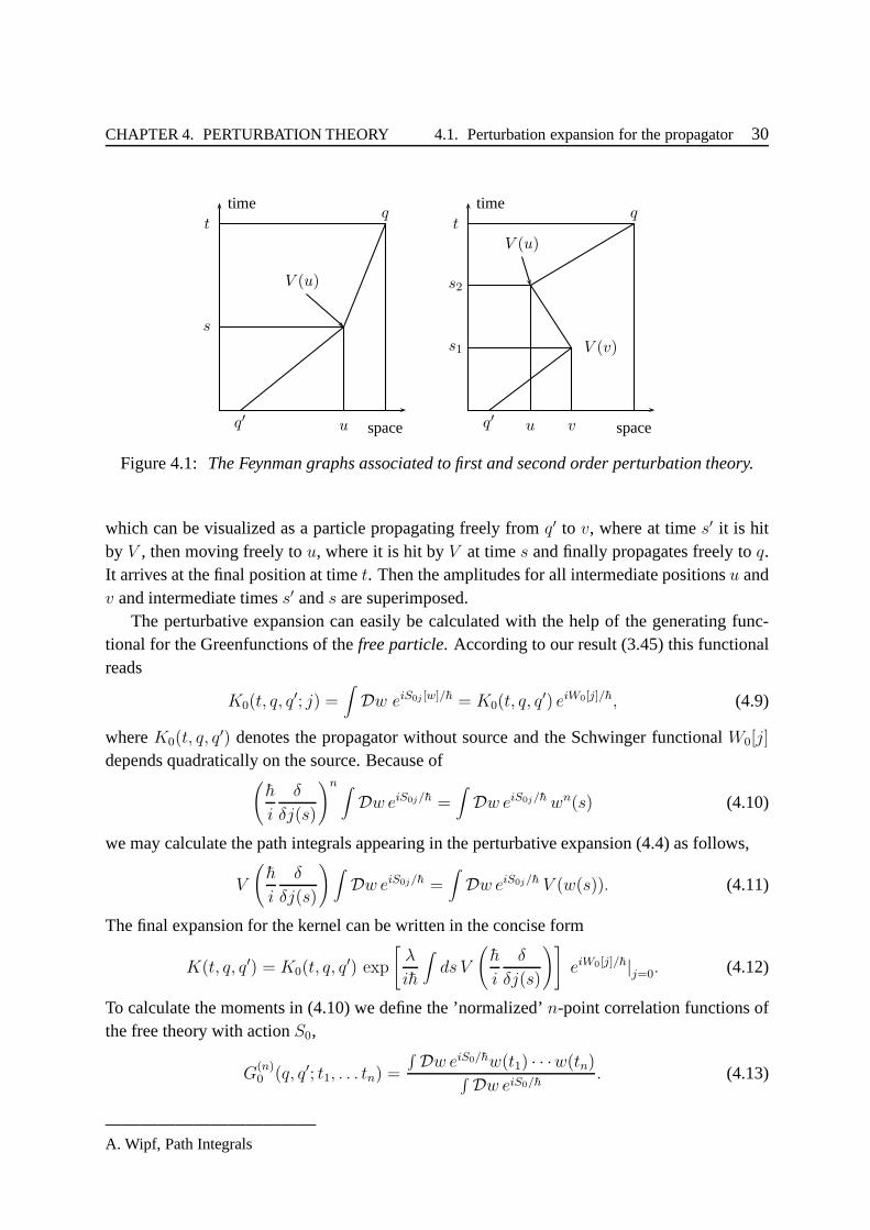
Figure 4.1: The Feynman graphs associated to first and second order perturbation theory.
which can be visualized as a particle propagating freely from q′ to v, where at times′ it is hitby V , then moving freely tou, where it is hit byV at times and finally propagates freely toq.It arrives at the final position at timet. Then the amplitudes for all intermediate positionsu andv and intermediate timess′ ands are superimposed.
The perturbative expansion can easily be calculated with the help of the generating func-tional for the Greenfunctions of thefree particle. According to our result (3.45) this functionalreads
K0(t, q, q′; j) =
∫
Dw eiS0j [w]/h = K0(t, q, q′) eiW0[j]/h, (4.9)
whereK0(t, q, q′) denotes the propagator without source and the Schwinger functionalW0[j]
depends quadratically on the source. Because of(
h
i
δ
δj(s)
)n ∫
Dw eiS0j/h =∫
Dw eiS0j/h wn(s) (4.10)
we may calculate the path integrals appearing in the perturbative expansion (4.4) as follows,
V
(
h
i
δ
δj(s)
)∫
Dw eiS0j/h =∫
Dw eiS0j/h V (w(s)). (4.11)
The final expansion for the kernel can be written in the concise form
K(t, q, q′) = K0(t, q, q′) exp
[
λ
ih
∫
ds V
(
h
i
δ
δj(s)
)]
eiW0[j]/h|j=0. (4.12)
To calculate the moments in (4.10) we define the ’normalized’n-point correlation functions ofthe free theory with actionS0,
G(n)0 (q, q′; t1, . . . tn) =
∫ Dw eiS0/hw(t1) · · ·w(tn)∫ Dw eiS0/h
. (4.13)
————————————A. Wipf, Path Integrals

CHAPTER 4. PERTURBATION THEORY 4.1. Perturbation expansion for the propagator 31
In our notation we made the dependence on the end points for the path over which one integratesexplicit. Inserting the result (4.9) for the generating functional the normalized correlation func-tions take the simple form
G(n)0 (q, q′; t1, . . . , tn) =
(
h
i
δ
δj(t1)· · · h
i
δ
δj(tn)
)∣∣∣j=0
eiW0[j]/h. (4.14)
Using the explicit form ofW0[j] in (3.44) theG(n)0 can be calculatedexplicitly. Actually, since
W0 is a quadratic functional ofj they can be expressed in terms of the1 and2-point correlationfunctions. The formulas expressing the highern-point functions in terms of the1 and2-pointfunctions is the celebratedTheorem of Wick.
In caseq′ = q = 0 the homogeneous solutionwh vanishes for all times and the theoremtakes a much simpler form, since the generating functional simplifies to
eiW0[j]/h =∞∑
n=0
1
n!
(i
2h
∫ t
0j(s)GD(s, s′) j(s′)
)n
. (4.15)
To simplify our notation we denote the Greenfunctions withq′ = q = 0 byG(n)0 (0, t1, . . . , tn).
Since the functional contains even powers ofj only, theG(n)0 vanish for oddn. The first non-
vanishing correlation function is
G(2)0 (0, t1, t2) =
h
iGD(t1, t2). (4.16)
For general evenn the Greenfunction is given by a sum of products of the two-point function,
G(2n)0 (0, t1, . . . , tn) =
∑
pairs (i1i2)···(i2n−1i2n)
G(2)0 (0, ti1, ti2) · · ·G(2)
0 (0, ti2n−1 , ti2n), (4.17)
where two indices in the sum are unequal and the pairs are ordered. This is theWick theoremfound in most text books and it holds for all theories with quadratic actions. For example, the4-point function contains3 terms
G(4)0 (0, t1, . . . , t4) = G
(2)0 (0, t1, t2)G
(2)0 (0, t3, t4)
+ G(2)0 (0, t1, t3)G
(2)0 (0, t2, t4) (4.18)
+ G(2)0 (0, t1, t4)G
(2)0 (0, t2, t3).
For all theories with quadratic action the generating functionalW [j] is quadratic inj and thetruncatedor connected correlation functions
G(n)c (q, q′; t1, . . . , tn) =
i
h
n∏
k=1
(
h
i
δ
δj(tk)
)
W [j]|j=0 (4.19)
vanish forn > 2. This simple observation then just proves the theorem of Wick.
————————————A. Wipf, Path Integrals
CHAPTER 4. PERTURBATION THEORY 4.2. Quartic potentials32
4.2 Quartic potentials
In order to calculate the corrections to the evolution kernel in first order perturbation theory(4.5) for a quartic potentialV = q4 we must determine
K1(t, q, q′) =
λ
ih
∫
ds∫
Dw eiS0[w]/hw4(s), (4.20)
where one integrates over paths withq(0) = q′ andq(t) = q. The last path integral is generatedbyK0(t, q, q
′, j) in (3.45) such that
∫
Dw eiS0/h w4(s) =
(
h
i
δ
δj(s)
)4
eiW0[j]/h∣∣∣j=0K0(t, q, q
′). (4.21)
Here we apply Wick’s theorem and obtain
(
h
i
δ
δj(s)
)4
eiW0[j]/h∣∣∣j=0
= 3G(2)(s, s)G(2)(s, s) + 6G(2)(s, s)w2h(s) + w4
h(s), (4.22)
where the2-point functionG(2) = hiGD and the homogeneous solutionwh for the free particle
have been calculated earlier in (3.43),
G(2)(s, s) =h
imt(s− t)s and wh(s) =
1
t[sq′ + (t− s)q]. (4.23)
To computeK1 we just need to integrate the fourth order polynomial in (4.22) which results in
K1(t, q, q′) = λK0(t, q, q
′)
ih
m2
t3
10+
3
m
t2
10(q2 + q′
2+
4
3qq′)
− i
h
t
5(q4 + q3q′ + q2q′
2+ qq′
3+ q′
4)
. (4.24)
We can trust the perturbative expansion ifK1 ≪ K0, which is the case if
λ≪ maxm2
ht3,m
t2q2,h
tq4
.
The expansions becomes reliable for short propagation times t and smallq′ andq. It breaksdown for small particle masses. According to Wicks theorem the higher order contributions inthe perturbative series (4.4) reduce to integrals of products of1 and2-point functions of the freeparticle. Hence they can be calculated in closed form. However, the number of terms one mustinclude grows rapidly with increasing ordern.
The perturbative expansion for the Greenfunction〈q, t|Tq(t1) · · · q(tn)|q〉 is obtained sim-ilarly as for the evolution kernel. Again we assume thatS is the sum of a free partS0 and an
————————————A. Wipf, Path Integrals
CHAPTER 4. PERTURBATION THEORY 4.2. Quartic potentials33
interaction termSI , see (4.2). Now we expand the right hand side of (2.48) in powers of thecoupling constantλ. This leads to the expansion
〈q, t|T q(t1) · · · q(tn)|q′〉
=∑ 1
n!
(
λ
ih
)n ∫
ds1 . . . dsn 〈q, t| q(t1) · · · q(tn)V (q(s1)) · · ·V (q(sn))|q′〉0 .
The matrix elements on the right hand side are to be evaluatedfor the system without interactionwhich means for the system with actionS0. Formally this series can be summarized as follows
〈q, t|T q(t1) · · · q(tn)|q′〉 = K0(t, q, q′) ·
n∏
k=1
(
h
i
δ
δj(tk)
)
exp
[
λ
ih
∫
ds V
(
h
i
δ
δj(s)
)]
eiW0[j]/h∣∣∣j=0
, (4.25)
with Schwinger functionW0[j] for the non-interacting system, see (3.44). SinceW0 is quadraticin the sourcej we may use Wick’s theorem to calculate the perturbative expansion on the righthand side.
————————————A. Wipf, Path Integrals
Chapter 5
Particles in electromagnetic fields
In this section study the dynamics of a charged particle in a given external electromagnetic field.In reality the field is modified by a moving charge, for exampleby the radiation emitted by theparticle. But here we shall neglect this backreaction. Thisis a reasonable approximation forstrong or/and almost constant fields.
5.1 Charged scalar particle
In classical physics we use the concept of an idealized pointparticle with massm and electricchargee. Such a particle moves along a trajectory and its position ata given time is determinedby its initial conditions and the equation of motion. On a particle at a positionx with velocityx acts the Lorenz force
F = e(
E (t, x ) +1
cx ∧B(t, x )
)
. (5.1)
To write down a Lagrangian or Hamiltonian function which lead to the corresponding equationof motion one introduces theelectromagnetic potentialsϕ andA in
E = −∇ϕ− 1
c
∂
∂tA , B = ∇∧A. (5.2)
Two potentials related by agauge transformationwith gauge functionλ(t, x ),
A(t, x ) → A(t, x ) −∇λ(t, x )
ϕ(t, x ) → ϕ(t, x ) +1
c
∂
∂tλ(t, x ) (5.3)
give rise to the same electromagnetic field. The non-relativistic Lorentz equationmx = F isthe Euler-Lagrange equation for the Lagrangian
L =m
2x 2 +
e
cx ·A(t, x ) − eϕ(t, x ). (5.4)
34

CHAPTER 5. PARTICLES INE AND B FIELDS 5.1. Charged scalar particle35
A Legendre transformation leads to the classical Hamiltonian function
H =1
2m
(
p− e
cA(t, x )
)2+ eϕ(t, x ), (5.5)
and with the help of the correspondence principle we arrive at the Hamiltonian operatorH andtime-dependent Schrodinger equation
id
dt|ψ(t)〉 = H|ψ(t)〉 , H =
1
2m
(
p− e
cA(t, x )
)2+ eϕ(t, x ). (5.6)
The operator-ordering is chosen such thatH gives rise to a unitary time evolution. Under agauge transformation (5.3) the wave function transforms as
ψ(t, x ) −→ e−ieλ(t,x )/hcψ(t, x ). (5.7)
If ψ fulfills the time-dependent Schrodinger equation with potentialsϕ andA then the gauge-transformed wave function fulfills the Schrodinger equation with gauge-transformed potentials.According to the general rules we expect that the path integral representation for the propagationof a charged particle from(t′, x ′) to (t, x ) in an electromagnetic field is given by
K(t, x , t′, x ′) =∫
Dw eiS[w ,A]/h, S =∫ t
t′ds(m
2w 2 +
e
cw ·A− eϕ
)
, (5.8)
where the values of the potentials along the particle path enter, for exampleϕ = ϕ(t,w(t)). Toprove that this propagator satisfies the time dependent Schrodinger equation we proceed simi-larly as in section 2.3 and replace the time-integral (5.8) by a Riemann sum. In the discretisationof the integral
∫
ds w ·A we must choose themidpoint rule,
∫
ds w(s) ·A(s,w(s)) −→n−1∑
j=0
ǫwj+1 − wj
ǫ·A
(sj+1 + sj
2,wj+1 + wj
2
)
(5.9)
with wj = w(sj). This corresponds to the socalledIto-calculus in the theory of stochasticdifferential equations. If we would take the potential atwj instead of the midpoint betweenwj
andwj+1 then we would obtain a gauge non-invariant propagator.Now we take a wave function at timet− ǫ and let it be propagated towardt. If u = x − y
denotes the difference between the final and initial position then we obtain up to terms ofO(ǫ2)
ψ(t, x ) ≈ limǫ→0
A3ǫ
∫
d3u exp(im
2hǫu2)
exp(iǫ
hLint
)
ψ(t− ǫ, x − u)
Lint =e
c
u
ǫ·A
(
t− ǫ
2, x − u
2
)
− eϕ(
t− ǫ
2, x − u
2
)
, (5.10)
As earlierAǫ = (m/2πihǫ)1/2 enters as normalizing factor. Expanding the two last factors inthe first line up to terms linear inǫ or quadratic inu . We obtain
ψ(t, x ) = limǫ→0
A3ǫ
∫
d3u expim
2hǫu2
ψ(t− ǫ) +1
2uiujDiDjψ − ieǫ
hϕψ + . . .
, (5.11)
————————————A. Wipf, Path Integrals

CHAPTER 5. PARTICLES INE AND B FIELDS 5.1. Charged scalar particle36
where we are lead to thecovariant derivative
D = ∇− ie
hcA. (5.12)
The potentials and wave function between the last curly brackets in (5.11) are taken at thepositionx . With the help of the Gaussian integrals
∫
d3u expim
2hǫu2
=1
A3ǫ
and∫
d3u expim
2hǫu2
uiuj =1
A3ǫ
ihǫ
mδij (5.13)
we obtain in the limitǫ→ 0 the partial differential equation
ih∂
∂tψ(t, x ) = − h2
2m(D2ψ)(t, x ) + eϕ(t, x )ψ(t, x ), (5.14)
which is just the Schrodinger equation (5.6) in the position representation. It is a useful exerciseto show that if we do not take the midpoint rule in (5.9) then wewould get a different result.Actually for the scalar potential and for the time-integration no midpoint rule is needed. Wewould still get the correct propagator in the continuum limit if we would take
Lint =e
c
u
ǫ·A
(
t, x − u
2
)
− eϕ (t, x ) , (5.15)
instead ofLint in (5.10). But with the choice (5.10) the convergence to the continuum limit isfaster. Under a gauge transformation (5.3) with gauge function λ(t, x ) the action changes bypath independent boundary terms,
∆S[w , A, ϕ] = −ec
∫ t
t′ds
(
w · ∇λ+∂
∂sλ
)
= −ecλ(t, x ) − λ(t′, x ′) (5.16)
such that the propagator transforms covariantly under gauge transformations,
K(t, x ; t′, x ′) −→ e−ieλ(t,x )/hcK(t, x , t′, x ′) eieλ(t′,x ′)/hc. (5.17)
This agrees with the transformation rule (5.7) for the solutions of the Schrodinger equationunder gauge transformations.
5.1.1 The Aharonov-Bohm effect
The Aharonov-Bohm effect demonstrates that in quantum mechanics a charged particle passingthrough a space region without electric and magnetic field can be influenced by electric andmagnetic fieldsoutsideof this region [16, 17]. In quantum mechanics the motion is describedby the Feynman path integral for the propagator (5.8) in which the potentials and not the fieldstrength enter. Even ifE andB vanish in some region of space,A need not vanish there due tothe presence of a magnetic field outside of the region.
————————————A. Wipf, Path Integrals

CHAPTER 5. PARTICLES INE AND B FIELDS 5.1. Charged scalar particle37
Here we consider the Aharonov-Bohm effect due to a magnetic fluxΦ confined to a solenoid.We assume that the solenoid is straight and very long and choose the coordinate system suchthat thez-axis is the symmetry axis of the solenoid. Outside the solenoid there in no magneticfield and for an infinitely long solenoid the magnetic potential has the form
A · dx =Φ
2π
xdy − ydx
ρ2, ρ2 = x2 + y2. (5.18)
We assume that the particle can not penetrate into the solenoid. Let us consider a particletrajectoryw(s) defining a curveC. The term containing the magnetic vector potential in theaction (5.8) is proportional to
∫ t
t′A(w(s)) · dw(s)
dsds =
∫
CA(x ) · dx =
Φ
2π
∫
C
xdy − ydx
ρ2. (5.19)
Transforming to cylinder coordinates(x, y, z) = (ρ cosϕ, ρ sinϕ, z) the line integral becomes∫
CA · dx =
Φ
2π
∫
Cdϕ. (5.20)
A pathCn : x ′ → x outside the solenoid is characterized by itswinding numbern ∈ Z. For itsdefinition one takes some standard contourC0 : x ′ → x and counts the number of times thatthe closed curveCn − C0 winds around the solenoid. In figure 5.1 we have depicted a reference
xb
C0
C1
x ′ b
∆ϕ
solenoid
Figure 5.1:A reference pathC0 and a pathC1 with relative winding1.
pathC0 and a pathC1 with winding number one. For a path with windingn one has∫
Cn
A · dx = nΦ +∫
C0
A · dx = nΦ +Φ
2π∆φ, (5.21)
————————————A. Wipf, Path Integrals

CHAPTER 5. PARTICLES INE AND B FIELDS 5.2. Spinning particles 38
where∆Φ is the angle shown in figure 5.1. In the path integral one admits all paths connectingx ′ with x . We do the integration in two steps: first we integrate over the set pathsCn withwinding numbern and then sum over all winding numbers. This yields
K(t, x , x ′) =∑
n
∫
CnDw eiS[w ,A]/h = eieΦ∆φ/hc
∑
n
eineΦ/hcKn(t, x , x′), (5.22)
whereKn is theA-independent topologically constrained Feynman path integral
Kn(t, x , x′) =
∫
CnDw exp
i
h
∫ t
0ds(m
2w 2 − eϕ(x )
)
ds
(5.23)
in which one integrates over trajectories which (when completed into a closed loop by continu-ing them with−C0) wind n-times around the solenoid. We see that no Aharonov-Bohm effectwill occur if the magnetic flux in the solenoid obeys the quantization condition
eΦ
hc= 0,±1,±2, . . . (5.24)
In this cases the phase factors containingn in (5.22) are unity and the summation overn gives
K(t, x , x ′) = exp(ieΦ
hc∆φ
)
K0(t, x , x′) (5.25)
whereK0 denotes the full, unconstrained, propagator for a particlein the absence of the mag-netic vector potential. If the magnetic flux does not fulfill the quantization condition (5.24) thenthe contributions of the various toplogical sectors to the propagator will interfere, and when ascreen is placed behind the solenoid the interference pattern on the screen will change whenΦis increased. This is the Aharonov-Bohm effect.
We have seen that the Aharonov-Bohm effect originates in theinteraction between the elec-tron and the external gauge potentialA whoseB-field vanishes locally. One can show that theeffect can equally well be regarded as originating in the interaction of the magnetic field of theelectron with the distantB-field inside the solenoid. From this point of view the effectis seento have a natural classical origin and loses much of its mystery [18].
5.2 Spinning particles
In the non-relativistic limit the wave function of a spin-12
particle has two components, it is aspinor, and correspondingly is the Schrodinger operator,calledPauli-Hamiltonianafter Wolf-gang Pauli, a2-dimensional matrix differential operator
H =1
2m
σ ·(
p− e
cA(t, x )
)2+ eϕ(t, x )12. (5.26)
————————————A. Wipf, Path Integrals

CHAPTER 5. PARTICLES INE AND B FIELDS 5.2. Spinning particles 39
Hereσ = (σ1, σ2, σ3) is the3-tuple of Pauli matrices. The Pauli-Hamiltonian contains acou-pling of the electron spin to a magnetic field with the correctg-factor of 2. Indeed, with the helpof σiσj = iǫikjσk + 12 the Pauli-Hamiltonian can be rewritten as
H =1
2m
(
p− e
cA(t, x )
)2+ eϕ(t, x ) − e
mcB(t, x ) · s , s =
h
2σ, (5.27)
where the two first terms act as identity operator in spin space. The corresponding matrix-valuedLagrange function
L =m
2x 2 +
e
cx ·A(t, x ) − eϕ(t, x ) +
e
mcB(t, x ) · s (5.28)
should enter the path integral for a non-relativistic spin-1/2 particle. AlthoughL is matrixvalued we could proceed as in the previous section and would end up with the result (5.10) withinteraction Lagrangian
Lint(t, x ,u) =(e
c
u
ǫ·A− eϕ+
e
mcB · s
)
midpoint. (5.29)
If the propagation is from(t−ǫ, x −u) → (t, x ) as it is in (5.10), then the midpoint rule meansevaluation of the potentials and magnetic field at timet − 1
2ǫ and positionx − 1
2u . This way
one obtains for the propagator the representation
K(t, x , t′, x ′) = limn→∞
A3nǫ
∫
d3w1 · · · d3wn−1 eiǫLn−1/h · · · eiǫL0/h,
Lj =m
2
u2j
ǫ2+e
c
uj
ǫ·A(sj, wj) − eϕ(sj, wj) +
e
mcB(sj, wj) · s , (5.30)
wherew0 = x ′, wn = x and we have used the abbreviations
uj = wj+1 − wj, wj =wj+1 + wj
2, sj =
sj+1 + sj2
. (5.31)
As earlier the propagation time interval[t′, t] is divided inton intervals of lengthǫ = (t− t′)/n
and sj = t′ + jǫ. For a time and/or space dependent magnetic field twoLj in (5.30) withdifferentj do not commute due to theB · s-term in the Lagrangian. In the (formal) continuumlimit we identify wj with the positionw(sj) of the particle at timesj . ThenLj is the value ofthe Lagrangian at timesj. We see that the factors in (5.30) are time ordered: on the right wehave the factorexp(iǫL0/h) at earliest time and on the left the factorexp(iǫLn−1/h) at latesttime. Thus we are lead to the path ordered integral
K(t, x , t′, x ′) =∫
Dw P exp(i
h
∫ t
t′dsL(s)
)
,
L(s) = L(
w(s),A(s,w(s)), ϕ(s,w(s)))
, (5.32)
————————————A. Wipf, Path Integrals

CHAPTER 5. PARTICLES INE AND B FIELDS 5.2. Spinning particles 40
where the time is ordered along the pathw(s). The path ordered integral satisfies the differentialequation
∂
∂tP exp
(i
h
∫ t
t′dsL(s)
)
=i
hL(t)P exp
(i
h
∫ t
t′dsL(s)
)
, (5.33)
and this equation together with the initial condition
P exp
(
i
h
∫ t′
t′dsL(s)
)
= 1 (5.34)
determines the path ordered integral.
5.2.1 Spinning particle in constantB-field
Let us consider a uniform magnetic field pointing in the direction of thez-axis,
A =B
2(xey − yex) ⇒ B = Bez. (5.35)
For a uniform magnetic field the action (5.28) for the spinning particle simplifies to
S =m
2
∫ t
0w 2 +
ω
2
∫ t
0B · (L + 2s), L = mw ∧ w , (5.36)
with cyclotron frequencyω = eB/mc. The particle moves freely in thez-direction and onlythe propagation in thexy-plane is affected by the external field. Thus we may assume that x ′
andx are both in the plane withz = 0 such that the whole tracetoryw(s) lies in this plane.Without loss of information we may study the two-dimensional dynamics in thexy-plane andin the following we assume that all vectors lie in the plane, for examplew = wxex + wyey.
For a uniform magnetic field the spin-term does not depend on the trajectory and hence doesnot enter the equation of motion. With the help of the rotation matrix
R(ωt) =
(
cosωt sinωt
− sinωt cosωt
)
(5.37)
the solution of the classical equation of motion can be written as
wcl(s) = x ′ +sin(ωs)
sin(ωt)R (ω(s− t)) (x − x ′), ω =
ω
2, (5.38)
and its action is given by
S[wcl] =mω
2cot(ωt)(x − x ′)2 −mω(xy′ − yx′) + ωt s3. (5.39)
————————————A. Wipf, Path Integrals
CHAPTER 5. PARTICLES INE AND B FIELDS 5.2. Spinning particles 41
The kinetic energy and the term containing the orbital angular momentum diverge if the propa-gation time is a multiple of2π/ω. Both contributions to the action contain a term proportionalto t/ sin2(ωt) and since they have different signs they cancel in the sum.
As earlier we decompose an arbitrary path asw(s) = wcl(s) + ξ(s), where the fluctuationsξ vanish at initial and final time. With
S[w ] = S[wcl] +m
2(ξ,Mξ), M = − d2
ds2+ iωσ2
d
ds, (5.40)
the path integral yields
K(t, x , x ′) =N√
detMeiS[wcl]/h. (5.41)
We remain with calculating the determinant of the matrix differential operatorM . This can beachieved by a generalization of the Gelfand-Yaglom initialvalue problem. One defines a matrixS, the columns of which are linearly independent solutions ofMξ = 0 vanishing ats = 0,
MS = 0 with S(0) = 0, S(0) = 1. (5.42)
Any solution ofMξ = 0, ξ(0) = 0 is a linear combination of the columns ofS. Let us nowassume that
detS(t) = 0. (5.43)
Then there is a linear combination of the columns ofS which vanish at the final timet. Itis an eigenfunction of the fluctuation operator with zero energy such thatdetM must vanish.Since the converse statement is also true, it is not surprising that the ratio of two fluctuationdeterminants is given by
detM
detM0=
detS
detS0=
1
t2det S. (5.44)
HereS0 = t1 is the matrix of solutions of the fluctuation operatorM0 with vanishingω. Inparticular for the fluctuation operator in (5.40) we have
S(t) = ω−1 sin ωt (cos ωt+ i sin ωt σ2) (5.45)
and this leads to the following ratio of determinants:
detM
detM0=
(
sin ωt
ωt
)2
. (5.46)
Inserting this result into (5.41) yields the well known propagator for a spinning particle in auniform magnetic field
K(t, x , x ′) =(
m
2πiht
)3/2 ωt
sin ωtexp
(im
2ht(z − z′)2 + iωσ3
)
× exp
imω
h
(
cot ωt
2
[
(x− x′)2 + (y − y′)2]
+ (x′y − xy′)
)
. (5.47)
————————————A. Wipf, Path Integrals

CHAPTER 5. PARTICLES INE AND B FIELDS 5.2. Spinning particles 42
To obtain the propagator in3 dimensions we have multiplied with the propagator for the freemotion in thez-direction. Similarly as for the harmonic oscillator the propagator is singularat timestn = 2πn/ω after which a classical particle returns to its starting point in the planeorthogonal to theB-field. Note that the two spin-components acquire differentphases in a non-vanishing magnetic field. The above result (without spin-term) has been obtained by GLASSER
[20] and by FEYNMAN and HIBBS [4].
————————————A. Wipf, Path Integrals

Chapter 6
Euclidean Path Integral
The oscillatory nature of the integrandeiS/h in the path integral gives rise to distributions. Ifthe oscillations were suppressed, then it might be possibleto define a sensible measure on theset of paths. With this hope much of the rigorous work on path integrals deals withimaginarytime t → −iτ for which the Lagrangian density undergoes the so-calledWick rotation. Oneanalytically continues to imaginary times, calculates thecorresponding Greensfunctions andcontinuous back to real time by the inverse Wick rotationτ → it. For imaginary time themeasure on the set of paths can rigorously be defined and leadsto theWiener measure.
6.1 Quantum Mechanics for Imaginary Times
For a selfadjoint Hamiltonian the unitary time evolution operator has the spectral representation
U(t) = e−iHt =∫
e−iEtdPE, (h = 1) (6.1)
where the integral has its support on the spectrum ofH. HerePE is the orthogonal projectoronto the subspace spanned by the eigenfunction with energy less or equal toE. We assume thatthe Hamiltonian is bounded from below and add a constant to it, such that it has non-negativespectrum. Then the above integral extends from0 to ∞. Now we assume thatt becomescomplext→ t− iτ ,
e−(τ+it)H =∫ ∞
0e−E(τ+it)HdPE. (6.2)
With our assumption this is a holomorphic semigroup in the half plane
t− iτ ∈ C, τ ≥ 0. (6.3)
If we would know the operator (6.2) for imaginary times(t = 0, τ ≥ 0) then we could analyt-ically continue it to real times(t, τ = 0), the time domain of interest in quantum mechanics.
43

CHAPTER 6. EUCLIDEAN PATH INTEGRAL 6.1. Quantum Mechanics for Imaginary Times 44
If we analytically continuet to −iτ then the Minkowskian metricη = diag(1,−1,−1,−1)
turns into a metric with Euclidean signature. This explainswhy this continuation is called thetransition from the Lorentzian- to the Euclidean sector of the theory.
The evolution operatorsU(t) are defined for all real times and form aone-parametric uni-tary group. It satisfies a Schrodinger equation
id
dtU(t) = HU(t), (6.4)
and its kernelK(t, q′, q) = 〈q|U(t)|q′〉 is complex and of oscillatory character. For imaginarytimes the ’evolution operators’
U(τ) = e−τH (6.5)
are positive (and hence hermitean instead of unitary) with non-negative eigenvalues. TheU(τ)
exist for positiveτ and form a so-called asemigroup. For almost all initial state vectors apropagation backwards in imaginary time is impossible.U(τ) satisfies adiffusiontype equation,
d
dτU(τ) = −HU(τ), (6.6)
and its kernel
K(τ, q, q′) = 〈q| e−τH |q′〉 with K(0, q, q′)) = δ(q, q′), (6.7)
is real for real Hamiltonians1. This kernel is strictly positive as follows from theTheorem: SupposeV is continuous and bounded from below, and letH = H0 + V be
essentially selfadjoint. Then the evolution kernel is positive,
K(τ, q, q′) = 〈q| e−τH |q′〉 > 0. (6.8)
If a (real) kernel would be negative forq′ in an open setO then we could construct a functionψ(q) ≥ 0 with support inO for which (ψ, U(τ)ψ) ≤ 0. This should not be possible for thepositive operatorU(τ). For a rigorous proof of (6.8) I refer to the textbook of Glimmand Jaffe[9], page 50. The positive kernel for a free particle ind dimensions reads
K0(τ, q, q′) =
( m
2πτ
)d/2e−m(q′−q)2/2τ , (6.9)
and the kernel for an oscillator with constant frequencyω is given byMehlers formula
Kω(τ, q, q′) =
( mω
2π sinhωτ
)d/2exp
− mω
2[(q2 + q′2) cothωτ − 2qq′
sinhωτ]
. (6.10)
1If we couple charged particles to a magnetic field, then the Hamiltonian ceases to be real.
————————————A. Wipf, Path Integrals
CHAPTER 6. EUCLIDEAN PATH INTEGRAL 6.1. Quantum Mechanics for Imaginary Times 45
The strict positivity of these kernels is manifest. This positivity allows for a deep connection ofEuclidean quantum mechanics (and field theory) to probability theory, see below. The object
P (τ, q) = C ·K(τ, q, 0) (6.11)
maybe interpreted asprobability densityfor a particle starting at0 to show up atq after a timeintervalτ . The probability to end up anywhere should be one,
C ·∫
dq 〈q, τ | 0, 0〉 = C ·∫
dqK(τ, q, 0) = 1, (6.12)
and this fixes the constantC. In particular, for the free particle
P0(τ, q) =( m
2πτ
)d/2e−mq
2/2τ . (6.13)
This is the probability density for theBrownian motionwith diffusion coefficientD = 1/2m. Itfulfils the same diffusion equation (6.6) asU(τ), in the present context calledmaster equation.
Wightman functions
Of great interest in a relativistic quantum field theory are the Wightman functions. These areexpectation values of product of field operators in the vacuum state. In quantum mechanicsthese are the expectation values
W (n)(t1, . . . , tn) = 〈Ω| q(t1) · · · q(tn)|Ω〉 , q(t) = eitH q e−itH , (6.14)
where|Ω〉 denotes the ground state. We subtracted the groundstate energy fromH such that|Ω〉has zero energy andH becomes a non-negative operator. TheW (n) are not symmetric in theirarguments, since the position operators at different timesdo not commute. We may analyticallycontinue theW (n) to zi → ti − iτi,
W (n)(z1, . . . , zn) = 〈Ω| qe−i(z1−z2)H qe−i(z2−z3)H q · · · q e−i(zn−1−zn)H q|Ω〉 , (6.15)
provided the imaginary parts of the complex time-differences obey the inequalities
ℑ(zk − zk+1) ≤ 0.
In equation (6.15) we used thatH annihilates the groundstate,exp(iζH)|Ω〉 = 0. From thedefinition of thezi it follows that theW (n) are analytic in
τ1 > τ2 . . . > τn. (6.16)
The Wightman functions for real times may be reconstructed as boundary values of the analyticWightman functions with complex arguments,
W (n)(t1, . . . , tn) = limℑzi→0
ℑ(zk+1−zk)>0
W (n)(z1, . . . , zn). (6.17)
————————————A. Wipf, Path Integrals
CHAPTER 6. EUCLIDEAN PATH INTEGRAL 6.2. The Euclidean Path Integral 46
For purely imaginary times the Wightman functions are called Schwinger functions,
S(n)(τ1, . . . , τ2) = W (n)(−iτ1, . . . ,−iτn)= 〈Ω| q e−(τ1−τ2)H qe−(τ2−τ3)H q · · · q e−(τn−1−τn)H q|Ω〉 . (6.18)
Let us calculate the2-point Wightman- and Schwinger functions of the harmonic oscillator. Thezero-point energy subtracted Hamiltonian reads
H = ωa†a,
wherea anda† are the lowering and raising operators
q =1√
2mω(a† + a) and p = i
√mω
2(a† + a) with [a, a†] = 1.
By construction the ground state|Ω〉 has zero energy and the first excited state|1〉 = a†|Ω〉 hasenergyE1 = ω. The two-point Wightman function only depends ont1 − t2 and reads
W (2)(t1 − t2) = 〈Ω| q(t1)q(t2)|Ω〉 =1
2mω〈Ω| (a+ a†)e−i(t1−t2)H(a + a†)|Ω〉
=1
2mω
⟨
a†Ω∣∣∣ e−itωa
†a∣∣∣a†Ω
⟩
=e−iω(t1−t2)
2mω, (6.19)
and the corresponding Schwinger function is
S(2)(τ1 − τ2) =e−ω(τ1−τ2)
2mω. (6.20)
In quantum field theory the Schwinger functions are invariant under the Euclidean LorentzgroupSO(4) which implies that they are symmetric in their arguments. This is not true in quantummechanics.
6.2 The Euclidean Path Integral
In this section we turn to the path integral formulation of quantum mechanics with imaginarytime. For that we recall, that the Trotter product formula (2.25) is obtained from the result(2.24) (which is used for the path integral representation for real times) by replacingit by τ .This is possible if the operators in this formula are boundedbelow. With the same arguments aswe used for real times we can now prove the analog of (2.29) foran imaginary time. The onlyeffect being thatiǫ is replaced byǫ. Thus one finds
K(τ, q, q′) = limn→∞
∫
dw1 · · ·dwn−1
(m
2πhǫ
)n/2
· exp
− ǫ
h
j=n−1∑
j=0
[m
2
(wj+1 − wjǫ
)2+ V (wj)
]
, (6.21)
————————————A. Wipf, Path Integrals

CHAPTER 6. EUCLIDEAN PATH INTEGRAL 6.3. Semiclassical Approximation 47
where as beforew0 = q′ is the initial position andwn = q the final position.The right hand side is identical to thepartition functionfor a one-dimensional lattice system
with sites labeled by the indexj and with fixed boundary conditions. The action in the exponentcouples nearest-neighbor variableswj andwj+1. The multiple integral is just a sum over allpossible lattice configurations. In this languageh is to be interpreted as temperature of thesystem and the classical limith → 0 corresponds to the low temperature limit of the latticesystem.
In the limit n→ ∞ the right hand side is a path integral, but now withEuclidean action
SE [w] =∫ τ
0dσ(m
2w 2 + V (w(σ))
)
(6.22)
and real and positive density
K(τ, q, q′) =
w(τ)=q∫
w(0)=q′
Dw e−SE [w]/h. (6.23)
The kernels for the free particle and the harmonic oscillator are given in (6.9) and (6.10).
6.3 Semiclassical Approximation
Here we discuss the semiclassical approximation for the evolution kernel. The small-h expan-sion of the Feynman path integral for real time is a stationary phase approximation whereas itis a saddle point approximation for imaginary time. We may recover the real-time kernelK(t)
from the imaginary-time kernelK(τ) by an analytic continuation in time. Since the saddle pointapproximation is easier to handle then the stationary phaseapproximation we shall consider theEuclidean path integral in what follows.
6.3.1 Saddle point approximation for ordinary integrals
As a warm up we study the saddle-point approximation forordinary integrals. Let us considerthe one-dimensional integral
K =∫ ∞
−∞dw e−αS(w). (6.24)
Hereα replaces1/h in the path integral. We wish to find a good approximation to this integral inthe limitα→ 0. Let us assume that the functionS in the exponent possesses a minimum atwcl.Then the main contribution to the integral comes from pointsnearwcl. ExpandingS(wcl + ξ)
about this minimum leads to
K = e−αS(wcl)∫
dξ e−12αS′′(wcl)ξ
2−αP (wcl,ξ), (6.25)
————————————A. Wipf, Path Integrals

CHAPTER 6. EUCLIDEAN PATH INTEGRAL 6.3. Semiclassical Approximation 48
whereP = o(ξ2) contains all higher order terms in the Taylor-expansion ofS about its mini-mum. Let us estimate therelative errorwe make when we approximateK by
Kn = e−αS(wcl)∫
dξ e−12αS′′(wcl)ξ
2n∑
k=0
(−)kαk
k!P (wcl, ξ)
k. (6.26)
We estimate the error relative to the quadratic approximationK0,
∆nK =K −Kn
K0
≡∫
dµα(ξ)
e−αP (ξ) −n∑
k=0
(−)kαk
k!P (wcl, ξ)
k
, (6.27)
where we have introduced theprobability measuredefined by the quadratic term in the Taylor-expansion of the functionS in the exponent,
dµα(ξ) =1
K0e−αS
′′(wcl)ξ2/2dξ =
√
αS ′′
2πe−αS
′′ξ2/2dξ. (6.28)
On the right hand side we abbreviatedS ′′ = S ′′(wcl). The measure satisfies the scaling relation
dµα(ξ) = dµ1(√αξ). (6.29)
We recall from the theory of Taylor series expansion, that for aCn+1-functionf(α) one has
f(α) −n∑
k=0
f (k)(0)αk
k!=f (n+1)(η)
(n+ 1)!αn+1 (6.30)
for some valueη in the interval[0, α]. Applied to the expression between the curly brackets in(6.27) we conclude that
. . . =(−α)n+1
(n+ 1)!P n+1e−ηP , with 0 ≤ η ≤ α. (6.31)
Without loss of generality we may assume thatP is non-negative such thatexp(−ηP ) is less orequal to one. Thus we can bound the relative error from above (6.27) as follows
|∆n−1K| ≤ αn
n!
∫
dµα(ξ)Pn(wcl, ξ). (6.32)
To extract theα-dependence of this bound we use the scaling relation (6.29)which implies
|∆n−1K| ≤ αn
n!
∫
dµ1(u)Pn(
wcl, u/√α)
. (6.33)
Recall thatP (wcl, ξ) contains the higher order terms in the Taylor expansion ofS and is of orderO(ξ3). From this we conclude that the relative error in (6.33) tends to zero for large values ofthe parameterα. For example, for a quartic functionP (ξ) = λξ4 the upper bound reads
|∆n−1K| ≤ 1
n!
(
λ
α
)n ∫
dµ1(u) u4n (6.34)
————————————A. Wipf, Path Integrals

CHAPTER 6. EUCLIDEAN PATH INTEGRAL 6.3. Semiclassical Approximation 49
which, with the help of the integral formula
∫
dµ1(u)u4n =
√
S ′′
2π
∫
e−S′′u2/2u4n =
(4n− 1)!!
(S ′′)2n
can be written in the form
|∆n−1K| ≤(
λ
α
)n(4n− 1)!!
n!
1
(S ′′)2n. (6.35)
We see that the saddle-point approximation becomes more accurate when the minimum is deepor the curvature at the minimum is large. Note that for a fixedα the error becomes arbitrarilybig for n→ ∞. With increasingn the parameterα must increase (orλ decrease) for the saddlepoint approximation to be applicable.
Inserting the Taylor series
e−αP =∞∑
m=0
(−)mαm
m!Pm
for a quarticP (ξ) into the complete integral we obtain the perturbation series
K
K0
=∫
dµα(w) e−αP (w) = 1 +∞∑
m=1
(−)m
(S ′′)2m
(4m− 1)!!
m!
(
λ
α
)m
≡∑
Am.
It is easy to see that the quotients of two successive terms inthis series grow withm,
Am+1
Am
m→∞−→ −λα· 16m
(S ′′)2(6.36)
which proves that the series has zero-radius of convergence. But from (6.35) it follows that it isstill an asymptotic series: for givenǫ andn there exists anα(n) such that for allα > α(n)
∣∣∣K
K0−
n∑
m=0
Am∣∣∣ < ǫ.
Note that for a non-convergent asymptotic seriesα(n) depends onn, contrary to the situation fora convergent series. Asymptotic series is the best we can hope for in a perturbative expansionof the propagator2. For the quartic functionS = w2/2 + λw4 with wcl = 0 the exact integral(6.24) forα = 1 is given by a modified Bessel function,
K = 2√κ eκK1/4(κ), κ = 1/32λ. (6.37)
The saddle point approximations of order3 is given by the polynomial
K3 =√
2π(
1 − 3λ+ 105λ2/2 − 3465λ3/2)
(6.38)
The exact result together with the approximationsK1, K2, K3 are depicted in figure 6.1.
2there is a general argument due to Dyson which shows that perturbative expansion cannot be analytic at thepoint where the coupling constant vanishes.
————————————A. Wipf, Path Integrals

CHAPTER 6. EUCLIDEAN PATH INTEGRAL 6.3. Semiclassical Approximation 50
0 0.05
K,Km
λ
√2π
2
exact
m = 1
m = 2
m = 3
Figure 6.1:The integralK for a quartic function and its lowest saddle point approximations.
6.3.2 Saddle point approximation in Euclidean Quantum Mechanics
To find the semiclassical approximation to the kernelK(τ, q, q′) we start with the path integralrepresentation (6.23), where the potential may include a source term. Note that for imaginarytime we can apply the saddle point approximation. For ordinary quantum mechanics with realtime we would perform a stationary phase approximation instead.
As for the ordinary integrals we expand the classical actionabout an extremum, that is abouta classical solution of the equation of motion
S ′E[wcl] = 0 ⇐⇒ mwcl = V ′(wcl), (6.39)
subject to the boundary conditions
w(0) = q′ and w(τ) = q. (6.40)
An arbitrary pathw(σ) is the sum of the classical path and a fluctuationξ(σ) and the Euclideanaction has the expansion
SE [wcl + ξ] = SE [wcl] +1
2(ξ, S ′′
E(wcl)ξ) + P [wcl, ξ], (6.41)
whereP contains all terms of cubic or higher orders
P [wcl, ξ] =1
3!
∫ τ
0V ′′′(wcl(σ))ξ3(σ) + · · · , (6.42)
————————————A. Wipf, Path Integrals

CHAPTER 6. EUCLIDEAN PATH INTEGRAL 6.3. Semiclassical Approximation 51
and the fluctuation operator has the explicit form
S ′′E(wcl) = −m d2
dσ2+ V ′′(wcl(σ)). (6.43)
Inserting these results into (6.23) yields
K(τ, q, q′) =
√
m
2πhD(τ)e−SE [wcl]/h
∫
dµh(ξ) e−P [wcl,ξ]/h, (6.44)
where one integrates over all fluctuating paths starting at the origin and returning to this pointafter a timeτ and theD-function in the first factor belongs to the fluctuation operator S ′′. Asfor the ordinary integrals we have introduced the Gaussian probability measure
dµh(ξ) =1
K0
e−(ξ,S′′E ξ)/2hDξ with K0 =
∫
Dξ e−(ξ,S′′Eξ)/2h. (6.45)
The relative errors are bounded by
|∆n−1K| =∣∣∣
∫
dµh
e−P/h −n−1∑
k=0
1
k!( − P/h)k
∣∣∣ ≤ 1
n! hn
∫
dµh Pn. (6.46)
Note that the measuredµh possesses the scaling property (6.29) withα replaced by1/h. Usingthis property for the quartic functionP = λ
∫
ξ4(σ)dσ one obtains
|∆n−1K| ≤ λnhn
n!
∫
dµ1(ξ)(∫
dσ ξ4(σ))n
. (6.47)
Since the path integral is calculated with the Gaussian measure withdµ1 it is independent ofh.This shows that the relative error∆n−1K is of the orderO(hn) for a quarticP .
The first correction to the classical contributionexp(−S[wcl]h) coming from the quadraticfluctuation is called the semiclassical correction orone-loop correction. According to (6.44) theone-loop approximation to the evolution kernel consistingof the classical part and the one-loopcorrection is
K0(τ, q, q′) =
√
m
2πhD(τ)e−SE [wcl]/h. (6.48)
The higher order terms can be computed systematically by calculating the corresponding mo-ments of the Gaussian measure defined by the fluctuation operator.
To determine the functionD appearing in the above expansions we first solve the classicalequation of motion with giveninitial positionq′ andinitial momentump′. Next we differentiatethe equation for the classical solutionwcl with respect to the initial momentum and obtain
md2
dσ2
dwcl
dp′= V ′′(wcl)
dwcl
dp′. (6.49)
————————————A. Wipf, Path Integrals
CHAPTER 6. EUCLIDEAN PATH INTEGRAL 6.4. Functional Determinants 52
For very short times the particles moves freely such thatwcl(σ) ∼ q′+p′σ/m+O(σ2) for smallσ. We conclude that
mdwcl
dp′(0) = 0 and m
d
dσ
dwcl
dp′(0) = 1. (6.50)
Sincemdwcl/dp′ obeys the same differential equation and the same initial condition as theD-
function the two functions must be identical. It follows that the 1-loop approximation to thekernel can be written as
K(τ, q, q′) =
(
2πhdwcl(τ)
dp(0)
)−1/2
e−SE [wcl]/h. (6.51)
This means that the correction to the classical result is given by the spread in the final positionof the classical particle (area where a projective may land)in terms of the spread in the initialmomentum (spread in the angle of projection). Thus, for artillery computation at least, it is animportant quantity!
The result can further be simplified by noting that the variation of the action when one variesthe end points is
δS = pq − p′q′ +∫
(−mw + V ′(w)) δw. (6.52)
For a classical trajectory the integral vanishes and we conluce that
∂Scl
∂q′= −p′ = −p(0). (6.53)
The variation of the initial momentum with respect to the final position is given by the secondvariation of the action of the classical trajectory (the Hamilton-Jacobi function) with respect tothe two end points
K(τ, q, q′) =1√2πh
(
− ∂2Scl
∂q′∂q
)1/2
e−SE [wcl]/h. (6.54)
This formula shows that it suffices to calculate the classical path for arbitrary endpointsq′ andq to calculate the1-loop approximation. According to (6.47) the1-loop result deviates from theexact answer at most by the termK0
∫
dµ1(ξ)P [wcl,√h ξ]/h.
6.4 Functional Determinants
In this section we shall study more carefully determinants of second order differential operatorswe did encounter in section 3.3, that is of the fluctuation operators of the form
M = M0 + U(s), where M0 =d2
ds2+ U0 (real time)
M = M0 + U(σ), where M0 = − d2
dσ2+ U0 (imag. time). (6.55)
————————————A. Wipf, Path Integrals

CHAPTER 6. EUCLIDEAN PATH INTEGRAL 6.4. Functional Determinants 53
HereU0 is either zero or a positive constant. The first determinant appears in ordinary quantummechanics and the second in Euclidean quantum mechanics. Such determinant show up in manyapplications of path integrals and it is worth studying these objects in detail.
If λn andλ0n are the eigenvalues ofM andM0, respectively, then both the numerator and
denominator in
detM
detM0=
∏λn
∏λ0n
=∞∞
are not well defined. Hence we consider the determinant of theratio of these two operators anddefine
detM
M0:=∏ λn
λ0n
, (6.56)
which in quantum mechanics at least leads to a finite and well-defined result. For example, forthe harmonic oscillator with frequencyω, the eigenvalues of the fluctuation operator on the timeinterval[0, t] or [0, τ ] are
λn(ω) = −(nπ
t
)2
+ ω2 or λn(ω) =(nπ
τ
)2
+ ω2 (6.57)
so that the infinite products (6.56), in which we skip the divergent factor withn = 0, are
real time:∏
n 6=0
λn(ω)
λn(0)=∏(
1 −( ωt
nπ
)2)
=sin(ωt)
ωt
imag. time:∏
n 6=0
λn(ω)
λn(0)=∏(
1 +(ωτ
nπ
)2)
=sinh(ωτ)
ωτ. (6.58)
Wedefinedthe determinant of the operatorM/M0 as the product of the ratios of the eigenvalues.These seems to be reasonable for commuting operatorsM andM0 which can be diagonalizedsimultaneously. For non-commuting operators it needs somefurther justification and this willbe given below. In the remainder of this this section the explicit calculations are done for realtime. The corresponding results for imaginary time are gotten by an analytic continuation.
Convergence of infinite products: Tor proceed we consider the one-parametric family offluctuation operators
Mα = M0 + αU(s), α ∈ [0, 1], (6.59)
interpolating between the operator without potentialM0 and the operator of interestM = M1.According to theFeynman-Hellman formulathe variation of an eigenvalueλ(α) is given by
d
dαλn(α) = (ψn(α), Uψn(α)), (6.60)
————————————A. Wipf, Path Integrals

CHAPTER 6. EUCLIDEAN PATH INTEGRAL 6.4. Functional Determinants 54
whereψn(α) is a normalized eigenfunction of the fluctuation operatorMα with eigenvalueλn(α). We immediately obtain the inequality
∣∣∣d
dαλn(α)
∣∣∣ ≤ Ω2, where Ω2 = max
s∈[t′,t]|U(s)|. (6.61)
Integrating these inequality with respect toα from 0 to 1 yields the following two inequalitiesfor the eigenvaluesλn of M and the eigenvaluesλ0
n of M0:
λ0n − Ω2 ≤ λn ≤ λ0
n + Ω2. (6.62)
For example, if we choose forM0 the operator∂2 with eigenvaluesλ0n = −(nπ/t)2 then these
inequalities yield the following upper and lower bounds forthe infinite product,
1
Ωtsin(Ωt) ≤
∏ λnλ0n
≤ 1
Ωtsinh(Ωt), (6.63)
where one of the inequalities becomes an equality for constant potentials. In particular we seethat the infinite products are always convergent. Actually,one can prove a stronger statement,namely that for anysquare-integrable potential
λn − λ0n =
1
t
∫ t
t′ds U(s) + rn
holds true, where the sum of ther2n exists. This inequality guarantees that the infinite product
in (6.56) converges.
From infinite products to determinants and traces: Now we wish to show that
∏ λnλ0n
= det(
1 + UM−10
)
(6.64)
can be defined in terms of the spectrum of the operatorUM−10 alone and that the definition
agrees with the previous one. This statement is not empty, since for non-commutingM andM0
their eigenfunctions may be rather different.The operatorA = UM−1
0 of interest is a socalledtrace class operator. These are operatorswith the property that tr|A| is finite, where|A| is the positive square root ofA†A. Trace-classoperators are compact and possess a discrete spectrumµ1 ≥ µ2, . . . and a representation
Aφn = µnφn +n−1∑
m=1
αnmφm, (φn, φm) = δmn. (6.65)
In the adapted basisφn a compact operator is represented by a triangular matrix with eigen-values on the diagonal. Now one defines the determinant of1 + A similarly as for matrices asthe product of the eigenvalues
det(1 + A) =∏
(1 + µn). (6.66)
————————————A. Wipf, Path Integrals

CHAPTER 6. EUCLIDEAN PATH INTEGRAL 6.4. Functional Determinants 55
The sum of the eigenvalues of a trace-class operator is absolute convergent [24]
∑
|µn| ≤ tr |A|.
It follows at once that the determinant of a trace-class operator is always finite and can easilybe bounded above as follows
det(1 + A) =∏
(1 + µn) ≤ exp(∑
|µn|)
≤ etr |A|. (6.67)
We see that for a trace-class operator the infinite product (6.66) is always absolute convergent3.From the definition of the determinant and the spectral decomposition (6.65) it is clear that
log det(1 +A) = tr log(1 +A). (6.68)
This formula will play an important role when we discuss the quantization of fermions in exter-nal fields or the one-loop effective actions for bosons.
Next we determine the variation ofdet(1 +A) if A is slightly perturbed by a trace class op-eratorǫB. Without loss of generality we may assume that the perturbedoperator is sufficientlysmall so that we may expand as follows
log det(1 +A+ ǫB) = tr log(1 +A+ ǫB)
= tr[
(A+ ǫB) − 1
2(A+ ǫB)2 + · · ·
]
= tr [ log(1 +A) + ǫ(1 + A)−1B +O(ǫ2)]
.
Thus we have shown that
d
dǫlog det(1 +A+ ǫB)|ǫ=0 = tr (1 + A)−1B. (6.69)
Now its easy to prove theproduct ruleapplies to the determinant of two operators,
det (1 + A)(1 +B) = det(1 + A) det(1 +B), (6.70)
which holds true for two trace-class operatorsA andB. To prove this product rule we multiplyAwith a deformation parameterα and show that theα-derivatives of the logarithm of both sidesin (6.70) are the same.
After these general remarks let us now prove the identity (6.64). Again we introduce adeformation parameter such thatM = M0 +αU and compute theα-derivative of the logarithmof the determinant appearing on the right hand side of (6.64). Using the identity (6.69) with
3More generally one can prove the following useful theorem: If for anyk>0 the series∑
µn,∑
µ2
n,∑
µk−1
n
and∑ |µn|k are convergent, then the infinite product
∏(1 + µn) is convergent as well.
————————————A. Wipf, Path Integrals
CHAPTER 6. EUCLIDEAN PATH INTEGRAL 6.4. Functional Determinants 56
A = UM−10 and the cyclicity of the trace (which holds for a trace-classand a bounded operator)
one sees at once that
d
dαlog det
(
1 + αUM−10
)
= tr UM−1. (6.71)
On the other hand, using again the Feynman-Hellman formula one can compute the variation ofthe logarithm of the infinite product in (6.64) directly as follows:
d
dα
∑
logλn(α)
λ0n
=∑ (ψn, Uψn)
λn= trUM−1. (6.72)
Comparing (6.71) with (6.72) we see that both sides of (6.64)possess the sameα-derivative.Since they are equal forα = 0 they must be equal forα = 1 and this proves (6.64) as required.
6.4.1 Calculating determinants
Let us now compute the functional determinants (6.64). We shall use the identity (6.71) andcompute the trace on the right hand side explicitly. To that end we introduce two fundamentalsolutionsC(s) andD(s) of
MC(s) = MD(s) = 0, M = M0 + αU, (6.73)
subject to the initial conditions
C(t′) = D(t′) = 1 and C(t′) = D(t′) = 0, (6.74)
so that their time-independentWronskianis
W (C,D) = CD − CD = 1. (6.75)
In terms of these fundamental solutions the Dirichlet Greenfunction forM reads fors < s′:
GD(s, s′) =C(t)
D(t)D(s′ )D(s) − C(s′)D(s). (6.76)
With this explicit expression for the Green function we can now calculate the trace in (6.71),
trUM−1 =∫ t
t′GD(s, s)U(s) =
C(t)
D(t)
∫ t
t′D2(s)U(s) −
∫ t
t′C(s)D(s)U(s). (6.77)
Let us finally define the function
W (t, t′) = D(t) trU M−1. (6.78)
————————————A. Wipf, Path Integrals

CHAPTER 6. EUCLIDEAN PATH INTEGRAL 6.4. Functional Determinants 57
It depends on the initial timet′ as well, but here we are interested in its dependence on the finaltime t and onα. By using (6.73) together with (6.75) one finds thatW obeys the differentialequation
(MW )(s) = −U(s)D(s), (6.79)
where the fluctuation operatorM acts ons. On the other hand, when differentiating (6.74) withrespect toα (recall thatM = M0 + αU) on obtains
M ∂αD(s, t′) = −U(s)D(s, t′) (6.80)
which shows thatW (t) and∂αD(t) are solutions of the same differential equation. Finallyit follows from the initial conditions (6.74) and from the representation (6.77,6.78) that bothfunctions and their first derivatives vanish att = t′ and thus we have
W (t) = ∂αD(t). (6.81)
Integrating the identity (6.72) fromα = 0 to α = 1 and noting that the infinite product is onefor α = 0 finally yields
log∏ λn
λ0n
= logD(t) − logD0(t), (6.82)
whereD is theD-function ofM = M0 + U andD0 that ofM0. Hence we end up with theexplicit result
detM
M0
=∏ λn
λ0n
=D(t)
D0(t), (6.83)
for the functional determinants appearing in the path integrals. Nowhere did we assume thatM0
is the free fluctuation operator such that the above formula holds true ifU0 in M0 = ∂2 + U0(t)
is time-dependent.We could have anticipated (6.83) by noting that
detM0 + αU
M0
is an analytic function ofα with simple zeros at values ofα for which one of the eigenvaluesλn(α) vanishes. For theseα the functionDα(s) vanishes att and is proportional to the cor-responding eigenfunction. Hence, the infinite product and the analytic functionDα(t) sharethe same zeros. Clearly, since forα = 0 the determinant is one, we must divideDα by theα-independentD0, but this normalization does not remove or add zeros/poles.According to atheorem by Weierstrass the quotientDα(t)/D0(t) must then be an analytic functionexp(f(α))
————————————A. Wipf, Path Integrals

CHAPTER 6. EUCLIDEAN PATH INTEGRAL 6.4. Functional Determinants 58
without zeros times the determinant. Finally from the asymptotic growth of the zeros ofDα onecan deduce thatf(α) = 0 and this proves (6.83).
What we have shown then is that the kernel (3.62) is given by
K(t, q, t′, q′) =
√
m
2πih(t− t′)
(
D0(t, t′)
D(t, t′)
)1/2
eiS[wcl]/h , (6.84)
whereD0(s, t′) andD(s, t′) are the Gelfand-YaglomD-functions belongingM andM0. They
fulfill the initial conditions
D(t′, t′) = D0(t′, t′) = 0 and
∂D(s, t′)
∂s
∣∣∣s=t′
=∂D0(s, t
′)
∂s
∣∣∣s=t′
= 1. (6.85)
For the free particleD0(s) = (s − t′) and its only role in (6.84) is to chancel thet − t′ in thesquare root. We thus recover our result for the kernel of the oscillator with time dependent forcein (3.21).
6.4.2 Generalizing the result of Gelfand and Yaglom
For a quantum mechanical system with several degrees of freedom is the fluctuation operatorM a matrix differential operator,
M = −1 d2
ds2+ P (s)
d
ds+Q(s), (6.86)
with matrix-functionsP andQ. Following KIRSTEN and MCKANE in [19] we convert thesecond order fluctuation problem
ξ = P ξ +Qξ (6.87)
into the equivalent first order problem
d
ds
(
ξ
ξ
)
= K
(
ξ
ξ
)
, K =
(
0 1Q P
)
. (6.88)
There are interesting applications where one needs the determinant ofM not only for Dirichletboundary conditions but for periodic, Neumann- or general Robin boundary conditions. Themost general linear boundary conditions can be written as
BL
(
ξ
ξ
)
(t′) +BR
(
ξ
ξ
)
(t) = 0 (6.89)
with ’boundary operators’BL andBR. For Dirichlet boundary conditions att′ andt we have
BL =
(1 0
0 0
)
and BR =
(
0 01 0
)
. (6.90)
————————————A. Wipf, Path Integrals

CHAPTER 6. EUCLIDEAN PATH INTEGRAL 6.4. Functional Determinants 59
To calculate the determinant of the fluctuation operatorM one solves theinitial value problem
d
dsψ = Kψ, ψ(t′) = 1. (6.91)
The columns of the matrixψ(s) form a complete set of linearly independent solutions of thefirstorder differential equation (6.88): any solution of this equation must be a linear combination ofthe columns ofψ. Let us assume that the determinant of
BLψ(t′) +BRψ(t)(6.91)= BL +BRψ(t)
vanishes. Then there exists a linear combination of the columns ofψ which satisfies the bound-ary condition (6.89). This linear combination gives rise a solution of the second order fluctua-tion problem (6.87) fulfilling the boundary conditions. This means thatdet(M) vanishes whenthe determinant ofBL +BRψ(t) vanishes. Since the converse statement holds as well, it is notsurprising that the ratio of two fluctuation determinants isgiven by [19]
detM1
detM2=
det(−∂2 + P1∂ +Q1)
det(−∂2 + P2∂ +Q2)=
det(BL +BRψ1(t))
det(BL +BRψ2(t)). (6.92)
For one degree of freedom and Dirichlet boundary condition with boundary operators (6.90)one recovers the original Gelfand-Yaglom formula for the ratio of functional determinants.
Zeta-function determinants
Finally we introduce another representation for determinants which is popular in field theory,namely thezeta-functiondefinition of determinants. The zeta-function of a (elliptic) selfadjointM is defined as
ζM(s) =∑
λ−sn = − 1
Γ(s)
∫
dt ts−1∑
e−tλn = − 1
Γ(s)
∫
dt ts−1tr e−tM , (6.93)
whereΓ(s) is the Riemann zeta-function. From the bounds (6.62) one infers that the difference
ζM(s) − ζM0(s) = −s∑
logλnλ0n
+O(s2)
is analytic at the origin and that its derivative at his pointis related to the determinant ofM/M0
as follows:
log detM
M0= −ζ ′M(0) − ζ ′M0
(0). (6.94)
The advantage of this representation is that one only needs to know the derivative of the zetafunction ats = 0 to compute the determinants of interest. In addition, the zeta-function defineddeterminants have some nice properties. In particular theyrespect a local gauge symmetry.Later we shall see that in certain field theoretical models (e.g. the massless Schwinger model)the valueζ ′M(0) can be calculated explicitly.
————————————A. Wipf, Path Integrals

Chapter 7
Brownian motion
The well-knownBrownian motionis a particular Gaussian stochastic process with covarianceE(wτwσ) ∼ min(τ, σ). There are many other known examples of Gaussian stochasticpro-cesses, for example the Ornstein-Uhlenbeck Process or the oscillator process. They all belongto a larger class of processes which are in general not even Gaussian and which we shall discussin the appendix.
The Brownian process describes the disordered motion of small particles suspended in aliquid. It is believed that Brown studied pollen particles floating in water under the microscope.He observed minute particles executing a jittery motion. The theory of this motion has beeninvented by EINSTEIN and SMOLUDCHOWSKI. The mathematically rigorous construction ofthe corresponding stochastic process has been developed byWIENER.
We have seen that contrary to the complex transitionamplitudeK(t, q, 0) in ordinary quan-tum mechanics, its continuationK(τ, q, 0) defines a probability density. For the free particlestarting at the origin the probability to end up atq after a ’time’τ is
P0(τ, q) =(m
2πτ
)d/2
e−mq2/2τ , (7.1)
and the probability to end up in the open setO ⊂ Rn is
P0(τ,O) =∫
Odq K0(τ, q, 0) ≤ 1. (7.2)
P0 belongs to aBrownian motion, named after the botanist ROBERT BROWN. Although themathematical model of Brownian motion is among the simplestcontinuous-time stochastic pro-cesses it has several real-world applications. An example is stock market fluctuations.
7.1 Diffusion
Diffusion is described byFick’s diffusion laws[25]. They were derived by ADOLF FICK inthe year 1855. The first law relates the diffusive flux to the concentration field, by postulating
60

CHAPTER 7. BROWNIAN MOTION 7.1. Diffusion 61
that the flux goes from regions of high concentration to regions of low concentration, with amagnitude and direction that is proportional to the concentration gradient,
J = −D∇φ. (7.3)
HereJ is the diffusion flux,D thediffusion coefficientwith dimensionm2/s andφ is the con-centration of the diffusing substance.D is proportional to the squared velocity of the diffusingparticles, which depends on the temperature and viscosity of the fluid and the size of the parti-cles according to theStokes-Einstein relation
D =kBT
γ, (7.4)
whereγ is the drag coefficient, the inverse of the mobility. For spherical particles of radiusr in a medium with viscosityη the drag coefficient isγ = 6πηr. In applications the drivingforce is a out of equilibrium concentration of particles, a spacial distribution of temperature ora non-vanishing gradient of a chemical potential.
Fick’s secondlaw predicts how diffusion causes the concentration field tochange with timeτ . It follows from his first law and the continuity equation
∂φ
∂τ= −∇ · J (7.5)
which expresses our expectation that the number of particles is conserved. The change of thenumber of particles in a given region is equal to the number ofparticles leaving or entering theregion through its boundary. Inserting the continuity equation into (7.3) yields the second lawof Fick,
∂φ
∂τ= ∇ · (D∇φ). (7.6)
For a constant diffusion coefficient D this law simplifies to
∂φ
∂τ= Dφ (7.7)
and it has the same form as theheat equation. An important example is the equilibrium case forwhich the concentration does not change in time, so that the left side of (7.7) is identically zeroandφ = 0. This is Laplace’s equation, the solutions to which are harmonic functions.
If we start at time0 with one particle atq′ the solution of (7.7) in denoted byK0(τ, q). Withthe initial condition
K0(0, q) = δ(q − q′) (7.8)
the solution of the diffusion equation is
K0(τ, q, q′) =
1√4πDτ
e−(q−q′)2/4Dτ (7.9)
————————————A. Wipf, Path Integrals

CHAPTER 7. BROWNIAN MOTION 7.2. Discrete random walk62
as can be verified by substitution. This has been known since the beginning of the last centuryand forms the subject of several textbooks on Brownian motion [26]. This particular solution isjust the Euclidean propagator (7.1) if we identifyD = 1/2m.
7.2 Discrete random walk
The Brownian motion is the scaling limit of adiscrete random walk. This means that if onetakes the random walk with very small steps one gets an approximation to Brownian motion.The one-dimensionaldiscrete random walk is the erratic motion of a point particle on a1-dimensional lattice with lattice spacinga. The particle suffers displacements in form of a seriesof steps, each step being taken in either direction within a certain period of time, say of lengthǫ.We suppose that forward and backward steps occur with equal probability 1
2and that successive
q0 q1 q2 q3q−1q−2q−3
ba
12
12
b
Figure 7.1:The particle may jump with equal probabilities one step to the left or right.
steps are statistically independent. Hence, the probability for a transition fromqj = ja toqk = ka during a timeǫ is
Pkj = P (ǫ, qk, qj) = 1
2if |k − j| = 1
0 otherwise.. (7.10)
This simple example of astochastic process(actually a Markov chain) is homogeneous andisotropic,
P (ǫ, qk, qi) = P (ǫ, qk − qi) and P (ǫ, qk, qj) = P (ǫ, qj , qk). (7.11)
After n time-steps the probability to jump fromqj to qk is given by the sum of the probabilitiesof the possible ways of achieving that, which is just
P (nǫ, qk, qj) =∑
i1,...in−1
Pki1Pi1i2 · · ·Pi2i1Pi1j = (P n)kj. (7.12)
The initial position of the particle may be uncertain and theprobability to find it at lattice pointqj is pj . If it sits with certainty1 at the origin thenpj = δj0. After n time-steps the systemhas evolved and produced a new distributionP np. The evolution operatorsP n determines thechange of the initial probability distribution aftern time-steps.
————————————A. Wipf, Path Integrals

CHAPTER 7. BROWNIAN MOTION 7.3. Scaling limit 63
It is not difficult to calculate the powers ofP . The probability to hop from the lattice siteqjto the siteqk aftern time-steps is1/2n times the number of paths on the lattice fromqj to qk. Ifn is even thenk−j must be even and ifn is odd thenk−j must be odd. The particle must jumpr = 1
2(n+ k − j) steps to the right andℓ = 1
2(n+ j − k) steps to the left. The number of paths
from qj to qk is then equal to the number of ways one can combiner steps to the right withℓsteps to the left to obtain a path of lengthn. This number is given by the binomial coefficient.Hence one finds the following probability
P (nǫ, qk − qj) =1
2n
(
n
r
)
=1
2n
(
n
ℓ
)
.
With the help of the identity(
n
r
)
+
(
n
r − 1
)
=
(
n+ 1
r
)
one obtains the difference equation
P (nǫ, q + a) + P (nǫ, q − a) = 2P (nǫ+ ǫ, q). (7.13)
whereq = qk − qj denotes the displacement. This equation maybe rewritten as
1
ǫP (τ + ǫ, q) − P (τ, q) =
a2
2ǫ
1
a2P (τ, q + a) − 2P (τ, q) + P (τ, q − a), (7.14)
whereτ = nǫ is the time during which the particle jumps.
7.3 Scaling limit
Now we regard the time-intervalǫ and lattice spacinga as being microscopic quantities andperform the scaling limit
a→ 0, ǫ→ 0 with nǫ = τ, D =a2
2ǫfixed. (7.15)
Other scaling limits are possible. For examplea → 0 with fixed ǫ would lead to a situationwhere the particle does not move anymore. The limita, ǫ → 0 with fixed a/ǫ would lead to aclassical theory without fluctuations. But if we keepa2/ǫ constant then the correlations tend tofinite values in this so-calleddiffusion limit. The constantD is the macroscopicdiffusion con-stant. In the macroscopic descriptionq andτ become continuous variables and the differenceequation (7.14) converts into a one-dimensional continuousdiffusion equation
∂
∂τP (τ, q) = D
∂2
∂q2P (τ, q). (7.16)
————————————A. Wipf, Path Integrals

CHAPTER 7. BROWNIAN MOTION 7.3. Scaling limit 64
At the initial time no diffusion has occurred andP (0, q) = δ(q). The solution of the diffusionequation with this initial condition is just the Gaussian function
P0(τ, q) = K0(τ, q, 0) =1√
4πDτe−q
2/4Dτ . (7.17)
The transition probability for the discrete random walk is replaced by the probability
limq′<qj<q
P (nǫ, qj) =1√
4πDτ
∫ q
q′du e−u
2/4Dτ . (7.18)
The trivial matrix identityP nPm = P n+m turns into theChapman-Kolmogorov equation∫
du P0(τ, q − u)P0(σ, u− q′) = P0(τ + σ, q − q′). (7.19)
Higher dimensions
The extension to higher dimensions is not difficult. For thatwe note that the lattice-Laplacianin one dimension acts on a function on the lattice as follows,
(Lf)(qj) =1
a2f(qj + a) − 2f(qj) + f(qj − a) (7.20)
such that the probability for a transition (7.10) can be rewritten as
P = 1 +a2
2L. (7.21)
Now we calculate then’th power ofP for n→ ∞ and use the scaling laws in (7.15)
P n =(
1 +a2
2
τ/n
ǫL
)n=(
1 +Dτ
nL
)n n→∞−→ e τD, (7.22)
wherelima→0 L = is the second derivative in the continuum. The kernel〈q, τ | eτD|0〉is just the above distributionP0(τ, q). Now the generalization tod dimensions is natural. Ifjenumerates the lattice points on ad-dimensional hypercubic lattice with lattice spacinga, thenthe matrixP is given by
Pij = 1
2di, j nearest neighbors
0 otherwiseor P = 1+
a2
2dL, (7.23)
whereL is the lattice Laplacian ind-dimensions, given by(
a2Lf)
(qj) =∑
k:|k−j|=1
f(qk) − 2d · f(qj). (7.24)
The factor1/2d in (7.23) is needed such that the probability to go somewhereis 1. In the scalinglimit we end up with a similar result as in one dimension,
limn→∞
P n = eτD, nǫ = τ,a2
2dǫ= D, (7.25)
and the Brownian motion tends to a Gaussian process with Laplacian.
————————————A. Wipf, Path Integrals
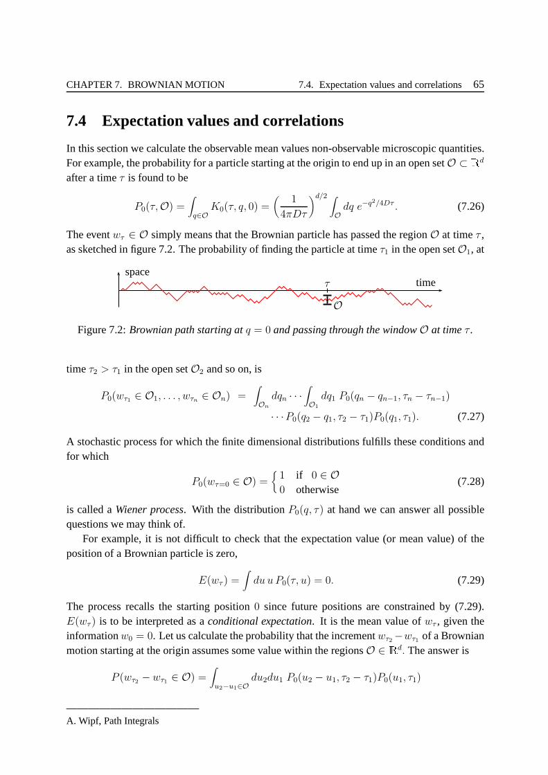
CHAPTER 7. BROWNIAN MOTION 7.4. Expectation values and correlations 65
7.4 Expectation values and correlations
In this section we calculate the observable mean values non-observable microscopic quantities.For example, the probability for a particle starting at the origin to end up in an open setO ⊂ Rd
after a timeτ is found to be
P0(τ,O) =∫
q∈OK0(τ, q, 0) =
(1
4πDτ
)d/2 ∫
Odq e−q
2/4Dτ . (7.26)
The eventwτ ∈ O simply means that the Brownian particle has passed the region O at timeτ ,as sketched in figure 7.2. The probability of finding the particle at timeτ1 in the open setO1, at
τ timespace
O
Figure 7.2:Brownian path starting atq = 0 and passing through the windowO at timeτ .
timeτ2 > τ1 in the open setO2 and so on, is
P0(wτ1 ∈ O1, . . . , wτn ∈ On) =∫
On
dqn · · ·∫
O1
dq1 P0(qn − qn−1, τn − τn−1)
· · ·P0(q2 − q1, τ2 − τ1)P0(q1, τ1). (7.27)
A stochastic process for which the finite dimensional distributions fulfills these conditions andfor which
P0(wτ=0 ∈ O) =
1 if 0 ∈ O0 otherwise
(7.28)
is called aWiener process. With the distributionP0(q, τ) at hand we can answer all possiblequestions we may think of.
For example, it is not difficult to check that the expectationvalue (or mean value) of theposition of a Brownian particle is zero,
E(wτ ) =∫
du uP0(τ, u) = 0. (7.29)
The process recalls the starting position0 since future positions are constrained by (7.29).E(wτ ) is to be interpreted as aconditional expectation. It is the mean value ofwτ , given theinformationw0 = 0. Let us calculate the probability that the incrementwτ2 −wτ1 of a Brownianmotion starting at the origin assumes some value within the regionsO ∈ Rd. The answer is
P (wτ2 − wτ1 ∈ O) =∫
u2−u1∈Odu2du1 P0(u2 − u1, τ2 − τ1)P0(u1, τ1)
————————————A. Wipf, Path Integrals

CHAPTER 7. BROWNIAN MOTION 7.5. Appendix A: Stochastic Processes 66
Changing variables fromu1, u2 to u1, v = u2 − u1 we can integrate overu1 and obtain
P (wτ2 − wτ1 ∈ O) = P (wτ2−τ1 ∈ O). (7.30)
The covariance for the one-dimensional process is
E(wτ wσ) =∫
d2u u2P0(u2 − u1, τ − σ) u1P0(u1, σ)
=1
2π√
det Σ
∫
d2u u2u1 e−(u,Σ−1u)/2,
where we assumed thatτ > σ and used a matrix notation
u =
(
u1
u2
)
, Σ = 2D
(
σ σ
σ τ
)
.
The resulting Gaussian integral yields
E(wτwσ) = Σ12 = 2Dσ = 2Dmin(τ, σ), (7.31)
where have already anticipated the result forτ < σ. For the Brownian motion in higher dimen-sions the corresponding result reads
E(wiτwjσ) = 2Dδij min(τ, σ). (7.32)
One can show that a typical trajectoryw(τ) of the Brownian motion is continuous. In dimensionone it is also recurrent, returning periodically to its origin. Indeed, one can prove the followingremarkable theorem:
Theorem: LetB(R, 0) ⊂ Rd be the ball with radiusR centered at the origin. Then
E (wτ ∈ B(R, 0) for oneτ) =
1 for d = 1, 2
< 1 for d ≥ 3.
The times of return of a one-dimensional Brownian motion canserve as a sophisticated randomnumber generator. As a mathematical model it does not only describe the random movement ofsmall particles suspended in a fluid; it can be used to describe a number of phenomena such asfluctuations in the stock market. Trajectories of a Brownianmotion are self-similar, a term thatis often used to describe fractals. Self-similarity means that for every segment of a given curve,there is either a smaller segment or a larger segment of the same curve that is similar to it.
7.5 Appendix A: Stochastic Processes
In this appendix we collect some useful facts about stochastic processes, since they are relatedto the Euclidean path integral. For proofs I refer to the extensive literature on measure theory,probability and stochastic processes [15]. First we need the definition of aprobability spaceconsisting of a triplet(Ω,A, P ).
————————————A. Wipf, Path Integrals

CHAPTER 7. BROWNIAN MOTION 7.5. Appendix A: Stochastic Processes 67
• The setΩ is asample space. An elementω ∈ Ω is called a simple event.
• The second entryA of the triplet denotes aσ-algebra of subsets ofΩ called events. Aσ-field is closed under complementation, countable intersections and unions,
A,B,Ai ∈ A =⇒ A\B ∈ A,∞⋃
i=1
Ai ∈ A, Ω ∈ A. (A.1)
• The third entryP is a probability measure. To any eventA ∈ A it assigns its probabilityP (A) ∈ [0, 1]. The probability of the empty set∅ is zero and that of the sample spaceΩ
is one. The measure has the following natural property
P ( ∪Ai) =∑
P (Ai) for Ai ∈ A, Ai ∩Aj = ∅, i 6= j. (A.2)
A functionX : A −→ Rd is calledBorel-measurable, if the preimage of any Borel set inRd
lies inA,
X−1(B) = ω ∈ Ω|X(ω) ∈ B ∈ A (A.3)
We recall that the Borel sets is the largestσ-algebra containing the open sets inRd. LetX beBorel-measurable on(Ω,A). ThenX is calledP -integrable, if
limn→∞
∞∑
k=0
k
nP
w :k
n< X(w) ≤ k + 1
n
≡ J+
limn→∞
0∑
k=−∞
k
nP
w :k − 1
n< X(w) ≤ k
n
≡ J−
both exist. Then one writes∫
ΩXdP = J+ − J− =
∫
X(ω) dP (ω). (A.4)
An A′-measurable mapX : A → A′ is calledrandom variable. If X is a random variable, thenevery measureP onA it defines a measurePX on the imageA′ as follows,
PX(A′) = P(
X−1(A′))
. (A.5)
PX is the distribution ofX with respect toP . One has the followingTheorem: For everyA′-measurable andPX integrable (numerical) functionf ′ onΩ′ the func-tion f ′ X isP -integrable,
∫
Ω′f ′dPX =
∫
Ω(f ′ X) dP. (A.6)
————————————A. Wipf, Path Integrals

CHAPTER 7. BROWNIAN MOTION 7.5. Appendix A: Stochastic Processes 68
Of particular importance are real-valued random variablesPX . They define measures on Borelsets inR. From the theorem one immediately concludes theLemma: If f is Borel measurable onR andX : Ω → R a real random variable, then
E(f X) =∫
Ω(f X) dP =
∫R fdPX (A.7)
In particular, theexpectation valueof a random variable is
E(X) =∫
w dPX(w), (A.8)
and its positivevarianceis given by
V (X) = E(
[X −E(X)]2)
= E(X2) −E2(X). (A.9)
LetXi, i = 1, . . . , n beR-valued random variables and
X1 ⊗ . . .⊗Xn : Ω −→ Rn, ω −→ (X1(ω), . . . , Xn(ω)). (A.10)
The corresponding induced measure for thejoint distributionis defined by
PX1⊗...⊗Xn(B1 × . . .× Bn) = P(
X−11 (B1) ∩ . . . ∩X−1
n (Bn))
. (A.11)
This should be contrasted with
(PX1 ⊗ . . .⊗ PXn) (B1 × . . .× Bn) = P(
X−11 (B1)
)
· · ·P(
X−1n (Bn)
)
. (A.12)
A number of random variablesX1, . . .Xn is calledindependentif
PX1⊗...⊗Xn = PX1 ⊗ . . . PXn =⇒ E(X1 · · ·Xn) = E(X1) · · ·E(Xn) (A.13)
holds true. Important and often used random variables are the Gaussian ones. A random variableis calledGaussianwith varianceΣ ≥ 0 and mean0 if
dPX(w) =1√2πΣ
e−w2/2Σ =⇒ E(X) = 0 and E(X2) = Σ. (A.14)
For a vanishing varianceΣ this simplifies toδ(w)dw. A set of Gaussain random variablesXi isjoint Gaussianwith meansE(Xi) = 0 and covarianceE(XiXj) = Σij if
PX1⊗...⊗Xn(w) =1
√
(2π)n det Σe−(w,Σ−1w)/2. (A.15)
After this preparations we introduce the notion of stochastic processes. Astochastic processisa family of random variables labelled by a (continuous) realparameter. In most application thisparameter is time. More accurately:
————————————A. Wipf, Path Integrals

CHAPTER 7. BROWNIAN MOTION 7.5. Appendix A: Stochastic Processes 69
Definition: A stochastic process is characterized by a quadruple(Ω,A, P, (Xτ)τ∈I), where(Ω,A, P ) is a probability space andXτ a family of random variables with values in a commonspace(E,B) of states. The parameter spaceI is typically the half line(0,∞). For every simpleeventω ∈ Ω the mapτ −→ Xτ (ω) is a path of the process.
For aGaussian stochastic processtheXτi have a joint Gaussian distribution for every finitesequenceτ1, . . . , τn. Let us relate this rather formal construction to the previously consideredBrownian motion. If we identifyw(τ) in (7.17) withXτ , then
P (τ, w) ∼ PXτ
in the present notation. The probability for finding the Brownian particle at timeτ in the intervalbetweena andb is
P (ω : a ≤ Xτ (ω) ≤ b) =∫ b
adPXτ (w). (A.16)
Similarly, the probability for finding the particle at timesτi betweenai andbi, where1 ≤ i ≤ n,is given by
P (ω : ai ≤ Xτi(ω) ≤ bi) =∫ b1
a1. . .∫ bn
an
dPXτ1⊗...⊗Xτn(w1, . . . , wn). (A.17)
Here one is naturally led to sets of the form
ω|(Xτ1 ⊗ . . .⊗Xτn(ω) ∈ B, B ∈ Bn.
If τ1, . . . , τn andn are arbitrary one obtains the set ofcylinder sets. They do not form aσ-algebra. In the theory of stochastic processes one uses theσ-algebra generated by this set.
Let us now indicate how one constructs a unique probability measure on the set of paths,that is how one performs the limit from joint distributions on a finite set of random variables toa induced probability measuredPXI
. The construction proceeds as follows:Let J be a subset of the parameter setI and define
EJ =∏
τ∈J
Eτ , Eτ = E and let BJ = ⊗τ∈J Bτ (A.18)
be the smallestσ-algebra inEJ such that the projections
pJ : EJ −→ E (A.19)
are measurable. For a finite setJ the elements ofEJ may be identified with the corners of abroken line path and for a continuousJ as a pathJ → E. TheBJ is then aσ-algebra on thesesets. In addition, letK be a subset ofJ . Then theprojections
pJK : EJ −→ EK , where K ⊂ J ⊂ I (A.20)
————————————A. Wipf, Path Integrals

CHAPTER 7. BROWNIAN MOTION 7.5. Appendix A: Stochastic Processes 70
areBJ − BK measurable. Next we consider the(EJ ,BJ) joint random variable
XJ = ⊗τ∈JXτ : Ω −→ EJ , Ω ∋ ω −→ pathXτ (ω), τ ∈ J
and letPXJdenote the joint distribution of random variablesXτ∈J . For example, for the set
J = (τ1, . . . , τn) this means
PXJ(B1 × . . .×Bn) = Pω|Xτ1(ω) ∈ B1, . . . , Xτn(ω) ∈ Bn.
SinceXK = pJK XJ we have
PXK= pJK(PXJ
). (A.21)
Now we need the following definition:Definition: If the family of probability measures(PXJ
) with finite J ⊂ I fulfills the condition
PXK= pJK(PXj
)
for two arbitrary finite subsetsK andJ with K ⊂ J , then the family is calledprojective. Nowone can prove the following important theorem
Theorem (Kolmogorov): IsE = Rn andB theσ-algebra of it Borel sets and ifI is a non-emptyset, then to each projective familyPXJ
of probability measures with finiteJ on (EJ ,BJ) thereexists exactly oneprobability measurePXI
on (EI ,BI) with
pJ(PXI) = PXJ
for all finite J.
One callsPXIthe projective limit of the familyPXJ
. The following theorems are useful:
Theorem: Let Σ(τ, σ) be a continuous and real-valued function onI×I, whereI is a separabletopological space. If for allτ1, . . . , τn the functionΣ(τi, τj) is positive semi-definite, thenthere exists a Gaussian process(Ω,A, P,Xτ) with covarianceΣ, that is
E (Xτ ·Xσ) = Σ(τ, σ).
To explain the following theorem, due to BOCHNER, we introduce thecharacteristic functionof a random variable,Definition: LetX be aRd-valued random variable. Then the Fourier transform of its measure,
φX(j) =∫
ei(j,w)dPX(w) = E(
ei(j,X))
(A.22)
is called thecharacteristic function. The measurePX is uniquely determined by the character-istic functionφX of the random variable. Now we can state the
————————————A. Wipf, Path Integrals

CHAPTER 7. BROWNIAN MOTION 7.5. Appendix A: Stochastic Processes 71
Theorem (Bochner): A functiona(j) is the characteristic function of a random variable if andonly if a(j) is continuous,a(0) = 1 and
∑
zia(ji − jj)zj ≥ 0 ∀j1, . . . , jn ∈ R; z1, . . . , zn ∈ C.The following theorem states, that under certain conditions the measure lives on the set ofcontinuous paths:
Theorem (Kolmogorov-Prehorov): Let(Ω,A, P,Xj⊂I) be a stochastic process. Then one maychange the random variables on a set of measure zero such thatthe new process(Ω,A, P, Xτ⊂I)
is continuous, provided that there exist real numbersa > 0, b > 1, c > 0 such that
E (|Xτ −Xσ|a) ≤ c|τ − σ|b, ∀ τ, σ ∈ R+.
One concludes that almost all (in the sense of measure theory) Brownian paths are continuous.One can also prove that almost all Brownian paths are nowheredifferentiable.
————————————A. Wipf, Path Integrals
Chapter 8
Path Integrals in Statistical Mechanics
The Feynman path integral formulation reveals a deep and fruitful interrelation between quan-tum mechanics and statistical mechanics. The discretized Euclidean path integrals can beviewed as partition functions for particular lattice spinmodels. Vice versa, the partition functionin statistical mechanics is given by a particular path integral with imaginary time. This unifiedview of quantum and statistical mechanics allows us to applymany powerful methods knownin statistical mechanics to calculate correlation functions in Euclidean quantum mechanics.
8.1 Thermodynamic Partition Function
In this section we derive a path integral representation forthe canonical partition function be-longing to a time-independent HamiltonianH. With our previous result in (6.23) we arrived atthe following Euclidean path integral representation for the kernel of the ’evolution operator’
K(τ, q, q′) = 〈q| e−τH/h|q′〉 =
w(τ)=q∫
w(0)=q′
Dw e−SE [w]/h. (8.1)
Here one integrates over all paths starting atq′ and ending atq. For imaginary times the inte-grand is real and positive and contains the Euclidean actionSE. Clearly, the object
∫
dqK(τ, q, q) = tr e−τH/h (8.2)
is just the quantumpartition functionfor temperaturekBT = h/τ . We conclude that the parti-tion functionZ(β) andfree energyF (β) at inverse temperature1 β = 1/T are given by
Z(β) = e−βF (β) = tr e−βH =∫
dq K(hβ, q, q). (8.3)
1We setkB = 1.
72

CHAPTER 8. STATISTICAL MECHANICS 8.2. Thermal CorrelationFunctions 73
Note that settingq = q′ in the last term means that we integrate over periodic paths starting andending atq in (8.1). Integrating overq is then equivalent to integrating overall periodic pathswith periodhβ. Thus we end up with
Z(β) =∮
w(0)=w(hβ)
Dw e−SE [w]/h . (8.4)
For example, for the Euclidean harmonic oscillator with evolution kernel (6.10)) we have
K(hβ, q, q) =
√
mω
2πh sinh(hωβ)exp
−2mωq2
h
sinh2(hωβ/2)
sin(hωβ)
, (8.5)
so that the partition function takes the form
Z(β) =1
2 sinh(hωβ/2)=
e−hωβ/2
1 − e−hωβ= e−hωβ/2
∞∑
n=0
e−nhωβ . (8.6)
For a Hamiltonian with discrete energiesEn the partition function has the spectral resolution
Z(β) = tr e−βH =∑
n
〈n| e−βH |n〉 =∑
n
e−βEn , (8.7)
where as orthonormal states|n〉 we used the eigenfunction ofH. A comparison with equation(8.6) immediately yields the energies of the harmonic oscillator with circular frequencyω,
En = hω(
n+1
2
)
, n ∈ N. (8.8)
For low temperatureβ → ∞ the spectral sum (8.7) is dominated by the contribution of lowestenergy such that the free energy will tend to the ground stateenergy,
F (β) = − 1
βlogZ(β)
β→∞−→ E0. (8.9)
To perform the high-temperature limit is more tricky. We shall investigate this limit later in thislecture. In applications one is also interested in the energies and wave functions of the excitedstates. Now we shall discuss a method to extract these quantities from the path integral.
8.2 Thermal Correlation Functions
The low lying energies of the Hamiltonian operatorH can be extracted from thethermal corre-lation functions. These are the expectation values of products of position operators
qE(τ) = eτH/hq e−τH/h, qE(0) = q(0), (8.10)
————————————A. Wipf, Path Integrals

CHAPTER 8. STATISTICAL MECHANICS 8.2. Thermal CorrelationFunctions 74
at different imaginary times in the equilibrium state at inverse temperatureβ,
〈qE(τ1) · · · qE(τn)〉β ≡ 1
Z(β)tr e−βH qE(τ1) · · · qE(τn). (8.11)
The normalizing factor in the denominator is the partition function (8.4). At temperature zerothese correlation functions are just theSchwinger functionswe introduced in section 6.1.
The gap between the energies of the ground state and first excited state can be extractedfrom the thermal 2-point function
〈qE(τ1)qE(τ2)〉β =1
Z(β)tr e−βH qE(τ1)qE(τ2)
=1
Z(β)tr e−(hβ−τ1)H/hq e−(τ1−τ2)H/hq e−τ2H/h (8.12)
as follows: we calculate the trace with the orthonormal energy eigenstates|n〉 and insert theidentity
∑|m〉 〈m| after the first position operator. Denoting the energy of|n〉 byEn we obtainthe following double sum for the thermal2-point function:
〈. . .〉β =1
Z(β)
∑
n,m
e−(hβ−τ1+τ2)En/he−(τ1−τ2)Em/h 〈n| q|m〉 〈m| q|n〉 . (8.13)
Now we consider the low-temperature limit of this expression. Forβ → ∞ the terms containingthe energiesEn>0 of the excited states are exponentially damped and we conclude
limβ→∞
〈qE(τ1)qE(τ2)〉β =∑
m≥0
e−(τ1−τ2)(Em−E0)/h | 〈Ω| q|m〉 |2. (8.14)
Note that the termexp(−βE0) chancels against the low temperatur limit of the partition functionin the denominator. At low temperature the thermal expectation values tend to the ground stateexpectation values,
limβ→∞
〈qE(τ1)qE(τ2)〉β = 〈Ω| qE(τ1)qE(τ2)|Ω〉 (8.15)
This just expresses the fact that thermal fluctuations freeze out at low temperature. Thermalexpectation values become vacuum expectation values at absolute zero. In particular the 1-point function has this property,
limβ→∞
〈qE(τ)〉β = 〈Ω| q|Ω〉 . (8.16)
At this point it is convenient to introduce theconnected thermal2-point function,
〈qE(τ1)qE(τ2)〉c,β = 〈qE(τ1)qE(τ2)〉β − 〈qE(τ1)〉〈qE(τ2)〉β . (8.17)
————————————A. Wipf, Path Integrals

CHAPTER 8. STATISTICAL MECHANICS 8.2. Thermal CorrelationFunctions 75
It characterizes the correlations of the differences∆qE = qE − 〈qE〉 at different times,
〈qE(τ1)qE(τ2)〉c,β = 〈∆qE(τ1) ∆qE(τ2)〉β . (8.18)
The connected correlator is exponentially damped for large|τ1 − τ2| since the term withm = 0
in (8.14) is missing in the spectral resolution for the connected2-point function,
limβ→∞
〈qE(τ1)qE(τ2)〉c,β =∑
m>0
e−(τ1−τ2)(Em−E0)/h| 〈Ω| q|m〉 |2. (8.19)
For large (imaginary) time-differencesτ1 − τ2 it reduces to
limτ1−τ2→∞
limβ→∞
〈qE(τ1)qE(τ2)〉c,β = e−(E1−E0)(τ1−τ2)/h| 〈Ω| q|1〉 |2, (8.20)
and thus one can extract the energy-gapE1 − E0 and modulus of the matrix element〈Ω| q|1〉from the large-time behavior of the connected 2-point function.
To find the path-integral representation for the thermal correlators we proceed similarly asin section 2.4. To calculate the two-point function (8.12) we insert the identity1 =
∫
du|u〉|u〉after the two position operatorsq in
Z(β) · 〈qE(τ1)qE(τ2)〉β =∫
dq 〈q| e−βH qE(τ1)qE(τ2)|q〉 , (8.21)
and in terms of the kernelK(τ, u, v) for the imaginary time evolution we obtain for the integrandin (8.21) the expression
〈q| . . .|q〉 =∫
dvdu 〈q|K(hβ − τ1)|v〉v 〈v|K(τ1 − τ2)|u〉u 〈u|K(τ2)|q〉 .
Now we use the path-integral representation for each evolution kernel separately, similarly aswe did for the Greensfunctions in section 2.4. Then the path-integral representation of the isevident: First we sum over all path fromq to u in timeτ2 and then multiply with the positionuof the particle at timeτ2. Next we sum over all path fromu to v in time τ1 − τ2 and multiplywith the positionv of the particle at timeτ1. Finally we sum over all path fromv to q in timehβ − τ1. The integration over the intermediate positionsu andv just means that we must sumover all paths, not only over those which have positionsu andv at timesτ2 andτ1, and include afactorq(τ1)q(τ2) in the integrand. Since the total traveling time of the particle ishβ, we obtainthe representation
〈q| e−βH qE(τ1)qE(τ2)|q〉 =
w(hβ)=q∫
w(0)=q
Dw e−SE [w]/hw(τ1)w(τ2), τ1 > τ2, (8.22)
for the kernel of the thermal 2-point function. Clearly, to get the trace in (8.12) we must inte-grate overq and then divide byZ(β) (whose path-integral representation we derived earlier).
————————————A. Wipf, Path Integrals
CHAPTER 8. STATISTICAL MECHANICS 8.2. Thermal CorrelationFunctions 76
Integrating overq means that we integrate overall periodic pathswith periodhβ. When weapplied the Trotter product formula we have assumed thatτ1 is bigger thanτ2. The path integralrepresentations for the higher ’time ordered’ thermal correlation functions is now evident,
〈T qE(τ1) · · · qE(τn)〉β =1
Z(β)
∮
w(0)=w(hβ)
Dw e−SE [w]/hw(τ1) · · ·w(τn). (8.23)
These correlators are generated by
K(hβ, q, q′; j) =
w(hβ)=q∫
w(0)=q′
Dw e−SEj [w]/h, SEj[w] = SE [w] − (j, w). (8.24)
or the corresponding generating functional, which is just the partition function in the presenceof an external sourcej(τ),
Z[β, j] =∫
dqK(hβ, q, q; j) =∮
w(0)=w(hβ)
Dw e−SEj [w]/h (8.25)
by differentiating with respect to the source. The source term (j, w) in (8.24) is the scalarproduct onL2[0, hβ]. Note thatZ(β, 0) = Z(β) is the previously introduced partition functionwithout source. For example, the thermal two-point function is
〈T qE(τ1)qE(τ2)〉β =1
Z(β, 0)
h2δ2
δj(t1)δj(t2)Z[β, j]|j=0, (8.26)
whereT denotes the time ordering.Theconnectedcorrelation functions are generated by thefinite-temperature Schwinger func-
tional. It is proportional to the logarithm of the partition function and hence proportional to thefree energy with external source,
logZ(β, j) = W [β, j]/h = −βF [β, j]. (8.27)
In many cases the source is just the applied magnetic field. Theconnected correlation functionsare gotten by functionally differentiatingW [β, j] several times with respect to the source,
〈T qE(τ1)qE(τ2) · · · qE(τn)〉c,β =hn−1δn
δj(τ1) · · · δj(τn)W [β, j]|j=0. (8.28)
Thermal Schwinger functional for the Oscillator
Let us compute the finite temperature Schwinger functional for the oscillator. We shall calculatethe path integral with Euclidian action and additional source term, that is for
SEj[w] =m
2
hβ∫
0
dτ
w2(τ) + ω2(τ)w2(τ)
−hβ∫
0
dτj(τ)w(τ). (8.29)
————————————A. Wipf, Path Integrals

CHAPTER 8. STATISTICAL MECHANICS 8.2. Thermal CorrelationFunctions 77
For later use we allow for a time-dependent frequency. We proceed similarly as in section 3.2where we calculated the propagator for the driven oscillator. Not to repeat ourselves we justrecall the key ideas and point out the main differences as compared to the previous calculation.First one splitsw into the classical pathwcl from q′ to q and the fluctuationξ(τ) which vanishesat the endpoints. The classical path is determined by the inhomogeneous equation of motion
S ′′wcl(τ) = j(τ), S ′′ = −m d2
dτ 2+mω2(τ), (8.30)
and the boundary conditionswcl(0) = q′ andwcl(hβ) = q. Expanding the actionSEj about thedominant classical path yields
K(hβ, q, q′; j) = e−SEj [wcl]/hK(hβ, 0, 0) = e−SEj [wcl]/h
√
m
2πhD(hβ), (8.31)
whereK(hβ, 0, 0) is the propagator for the propagation without source from0 to 0. TheD-function solvesS ′′D = 0 with initial conditionsD(0) = 0 andD(0) = 1. This formula is justthe Euclidean version of the result (3.32). Again we decompose the classical trajectory in twoparts,
wcl(τ) = wh(τ) +∫ hβ
0GD(τ, σ)j(σ)dσ, (8.32)
wherewh is the classical path fromq′ → q withoutexternal source andGD(τ, σ) is the symmet-ric Dirichlet Greenfunction of the fluctuation operatorS ′′. The second term on the right handside vanishes at initial and final times and solves the equation of motion with source. Using thisinformation the action ofwcl can be rewritten as
SEj[wcl] = SE [wh] − (j, wh) −1
2(j, GDj) . (8.33)
Now we insert this decomposition into (8.31). The termSE[wh] converts the source-free propa-gator for the propagation from0 → 0 in (8.31) into the source-free propagator for propagationfrom q′ to q such that
K(hβ, q, q′; j) = K(hβ, q, q′) · exp (j, GDj)/2h+ (j, wh)/h . (8.34)
In order to obtain the partition function we must setq′ = q and integrate overq. To do theintegration we need the explicitq-dependence of the actionSEj[wcl] in (8.33). To that aim weintroduce a particular solutionφ(τ) of the homogeneous equation of motion,
S ′′φ = 0 and φ(0) = φ(hβ) = 1. (8.35)
The classical solutionwh from q → q in the decomposition (8.32) is justwh(τ) = qφ(τ). Usingthe equation of motion and boundary conditions forφ the position dependent contributions toSEj in (8.33) can be isolated,
SEj[wcl] =1
2mβ q
2 − q(j, φ) − 1
2(j, GDj), (8.36)
————————————A. Wipf, Path Integrals

CHAPTER 8. STATISTICAL MECHANICS 8.2. Thermal CorrelationFunctions 78
where we introduced the source and position-independent function
mβ = mφ(hβ) −mφ(0). (8.37)
We see that the resulting propagatorK(hβ, q, q; j) is a Gaussian function ofq. Integrating overq we obtain the partition function in the presence of an source
Z[β, j] = Z(β) eW [β,j]/h (8.38)
whereZ(β) is the partition function of the oscillator,
Z(β) =
√
2π
mβK(hβ, 0, 0) (8.39)
andW the its finite temperature Schwinger functional,
W [β, j] =1
2(j, GP j), where GP (τ, σ) =
φ(τ)φ(σ)
mβ+GD(τ, σ). (8.40)
Actually GP is just the Greenfunction ofS ′′ for periodic boundary conditions. The term pro-portional toφ(τ)φ(σ) in (8.40) converse the Dirichlet Greenfunction into the periodic Green-function. This fact is proven in the appendix to the present chapter.
To compute th connected 2-point function at finite temperature we differentiateW [β, j]
twice with respect to the source and then set the source to zero. We obtain
〈TqE(τ1)qE(τ2)〉c,β = GP (τ1, τ2). (8.41)
Note that the partition functionZ(β) does not enter the result for the connected correlationfunction. For the oscillator with constant frequency the periodic Greenfunction reads
GP (τ, σ) =1
2mω
cosh(ω|τ − σ| − hωβ/2)
sinh(hωβ/2)(8.42)
and one obtains the following thermal two-point function
〈TqE(τ1)qE(τ2)〉β = hGP (τ1, τ2)β→∞−→ h
2mωe−ω|τ1−τ2|. (8.43)
Comparing with (8.20) we can extract both the mass gap and modulus of the matrix element ofq between ground state and first excited state,
E1 − E0 = hω and | 〈Ω| q|1〉 |2 =h
2mω, (8.44)
a familiar result from the quantum mechanics course.
————————————A. Wipf, Path Integrals
CHAPTER 8. STATISTICAL MECHANICS 8.3. Wigner-Kirkwood Expansion 79
8.3 Wigner-Kirkwood Expansion
The Wigner-Kirkwood expansion [27] can be used for studyingthe equilibrium statistical me-chanics of a nearly classical system of particles. It is a semiclassical expansion in powers ofPlanck’s constanth,
Z(β) = Zcl(β) +O(h2), Zcl(β) =
√
m
2πβh2
∫
dq e−βV (q), (8.45)
or equivalently of the thermal de Broglie wavelengthλ = h(β/m)1/2. The h-expansion forthe partition functionZ(β) = tr exp(−βH) is different from that for the evolution kernel inquantum mechanics. The small expansion parameterh entersZ(β) only via h2 in the kineticenergy whereas in the kernel〈q| exp(itH/h)|q′〉 it also enters as overall factor in the exponent.Here we shall derive the Wigner-Kirkwood expansion from thepath integral representation forthe partition function
Z(β) =∮
w(0)=w(hβ)
Dw e−SE [w]/h. (8.46)
The normalization of the (formal) path integral is fixed by the classical limitZcl(β) in (8.45).We rescale imaginary time such that the periodicity of the paths isβ instead ofhβ,
τ −→ hτ. (8.47)
After this rescaling of time the path integral reads
Z(β) =∫
w(0)=w(β)
Dw exp
−∫ β
0
[m
2w2/h2 + V (w)
]
dτ
. (8.48)
Observe that for a moving particle the kinetic energy dominates the potential energy for smallhwhereas for a particle at rest the potential term is dominant. This suggest to split a path into itsconstant part (for which the kinetic energy vanishes) and fluctuations about it. Thus we changevariables fromw(τ) → q + hξ(τ) such thatξ(0) = ξ(β) = 0. We obtain
Z(β) =∫
dq∫
ξ(0)=ξ(β)=0
Dξ exp
−m2
∫ β
0ξ 2dτ
exp
−∫ β
0V (q + hξ) dτ
. (8.49)
Now we expand the last exponential factor containing the potential in powers ofh,
exp . . . = e−βV
1 − hV ′I(ξ) +h2
2
(
V ′ 2I2(ξ) − V ′′I(ξ2))
− h3
3!
(
V ′ 3I3(ξ) − 3V ′V ′′I(ξ)I(ξ2) + V ′′′I(ξ3))
+ . . .
, (8.50)
————————————A. Wipf, Path Integrals

CHAPTER 8. STATISTICAL MECHANICS 8.3. Wigner-Kirkwood Expansion 80
where the argument ofV and its derivatives is the constant pathq and we abbreviated the timeintegrals of powers of the fluctuation field by
∫
ξn(τ)dτ ≡ I(ξn). (8.51)
The remaining path integral in (8.49) leads to correlators of the time integrated fluctuations, forexample
〈I(ξ2)I(ξ)〉 =∫
ξ(0)=ξ(β)=0
Dξ exp
−m2
∫
ξ 2 ∫
ξ2(τ)dτ∫
ξ(σ)dσ. (8.52)
The explicit form of the lowest order terms in the resulting series is
Z(β) =∫
dq eβV
〈1〉 − hV ′〈I(ξ)〉+h2
2
(
V ′ 2〈I2(ξ)〉 − V ′′〈I(ξ2)〉)
+ . . .
(8.53)
The expectation values (8.52) before time-integration aregenerated by the generating functionalof the free particle with Dirichlet boundary conditions andh = 1,
K(β, 0, 0; j) =
√
m
2πβexp
1
mβ
∫ β
0dτ∫ τ
0dσ (β − τ)σj(τ)j(σ)
. (8.54)
To determine the expansion up to orderh2 we need
〈1〉 =
√
m
2πβ, 〈ξ(τ)〉 = 0 and 〈ξ(τ)ξ(σ)〉 =
〈1〉mβ
(β − σ)τ (τ < σ). (8.55)
Finally we must integrate overτ (andσ) which, after a partial integration inq, leads to
Z(β) =
√
m
2πβh2
∫
dq e−βV (q)
(
1 − h2 β3
24mV ′ 2 +O(h4)
)
, (8.56)
where we have already anticipated that the odd powers ofh vanish in this expansion, since theodd moments of the free measure vanish.2
The first term in this power series inh is the classical partition function. The coefficients ofO(hn) contain exactlyn derivatives of the potential, e.g. theh4 coefficient contains terms like
V ′′′′, V ′ 4, V ′′′V ′ and V ′′ 2. (8.57)
We see that theh-expansion is actually a gradient expansion. A strongly coupled system be-haves classically and we may expect that its behavior is described by a Wigner-Kirkwood gradi-ent expansion. The first few terms in the semiclassical expansion have been derived by WIGNER
AND K IRKWOOD [27].
2One needs to restore an additional factor of1/h to find the correct classical limit. This is due to the differentrescaling of the constant path and the fluctuationsξ(τ).
————————————A. Wipf, Path Integrals

CHAPTER 8. STATISTICAL MECHANICS 8.4. High Temperature Expansion 81
8.4 High Temperature Expansion
Besides the perturbative expansion in the powers of the interaction term or the semi-classicalexpansion in powers ofh there exits another approximation of considerable interest, namely thehigh temperature expansion in powers of the inverse temperatureβ. Actually we shall need thisexpansion later when we discuss certain gauge field theoriesand in particular their anomalies.
The temperature dependence of finite temperature expectation values comes from theβ-periodicity (more accuratelyh/kBT -periodicity) of the trajectories in the path integral. As inthe previous section we split a path into its constant partq and the fluctuationsξ(τ) aboutq.This way the partition function becomes theq-integral over the fluctuation part,
Z(β) =∫
dq Z(β, q). (8.58)
The heat kernelK(β, q) is the path integral over the fluctuations in (8.49) (to simplify thenotation we seth = 1). Now we rescale time such the fluctuation have periodicity1 andat the same time rescale the amplitude of the fluctuations such the kinetic term becomesβ-independent:
τ −→ βτ and ξ −→√
β ξ. (8.59)
After these rescaling theβ-dependence comes only from the temperature-dependent potential:
Z(β, q) =1√β
∫
ξ(0)=ξ(1)=0
Dξ exp
−m2
∫ 1
0ξ2
exp
−β∫
V (q +√
β ξ) dτ
. (8.60)
Now we expand the last exponential in powers ofβ. Again we are lead to calculate time integralsof correlators of the fluctuation field. Using〈ξ(τ)〉 = 0 we find the following expansion for theheat kernel
Z(β, q) =√
β
⟨
1 − βV (q) +β2
2V 2(q) − β2
2V ′′(q) I(ξ2)
−β3
3!V 3 +
β3
2V ′V ′I2(ξ) +
β3
2V V ′′I(ξ2) − β3
24V ′′′′I(ξ4) . . .
⟩
. (8.61)
Inserting the correlators (8.55) withβ = 1 we can compute the remaining correlators and time-integrals. This way one obtains
Z(β, q) =
√
m
2πβ
1 − βV +β2
2V 2 − β2
12mV ′′
−β3
6V 3 +
β3
24mV ′V ′ +
β3
12mV V ′′ − β3
240m2V ′′′ + . . .
, (8.62)
————————————A. Wipf, Path Integrals
CHAPTER 8. STATISTICAL MECHANICS 8.5. High-T Expansion for/D2 82
where the potential and its derivatives are evaluated on theconstant pathq. The partition func-tion is the space integral of this kernel. If the potential islocalized near the origin or alternativelyif space is compact we obtain the series expansion
Z(β) − Z0(β) =
√
m
2πβ
∫
dq
−βV +β2
2V 2 − β3
6V 3 − β3
12mV ′ 2 + . . .
(8.63)
For very high temperature the particles move almost freely and as expectedZ(β) tends to thepartition functionZ0(β) of a gas of free particles with massm. Note that besides the overallfactorβ−1/2 the density and the partition function have an expansion in integer powers ofβ,although the argument ofV in (8.60) contains
√β. The corresponding expansion for a particle
propagating ind-dimensions reads
Z(β) − Z0(β) =
(
m
2πβ
)d/2 ∫
ddq
−βV +β2
2V 2 − β3
6V 3 − β3
12m(∇V )2 + . . .
. (8.64)
In [28] the high temperature expansion was completely computerized using the algebraic lan-guage FORM. The calculation was performed up to orderβ11. For the coefficient ofβn in theexpansion ofZ(β) the number of terms are:
n 7 8 9 10 11
# of terms 37 114 380 1373 5301
The high temperature expansion enters the inverse mass expansion of worldline path integralsoccuring in one-loop effective action.
8.5 High-T Expansion for the Dirac-Hamiltonian
The heat kernel expansion of the previous section is of greatimportance in relativistic quantumfield theories. The Lagrangian for the electron- or quark-field contains the Dirac operator/D andthe fermionic path integral leads to the determinant of thisoperator. This determinant in turncan be related to the partition function of− /D
2. Here we shall compute the high temperature
expansion of the heat kernel
Z(β, q) = 〈q| eβ /D2 |q〉 , (8.65)
where the Euclidean Dirac-operator
/D = γµDµ. (8.66)
contains thecovariant derivativewhich couples the fermionic field to the gauge potentialAµ,
Dµ = ∂µ − iAµ. (8.67)
————————————A. Wipf, Path Integrals

CHAPTER 8. STATISTICAL MECHANICS 8.5. High-T Expansion for/D2 83
In Quantum Electrodynamics (QED) the electric and magneticfields entering the field strengthtensorFµν are given byFµν = ∂µAν − ∂νAµ. In non-Abelian gauge theories the potentialAµand field strengthFµν are matrix values functions. They take their values in the Lie-algebraof the underlying gauge group. Besides the gauge potential the Dirac operator contains theEuclidean matricesγµ obeying the anti-commutation relations
γµ, γν = 2δµν , µ, ν = 1, .., d. (8.68)
In d dimensions they are2[d/2]-dimensional hermitian matrices. The explicit form of the secondorder hermitian matrix differential operator/D
2is
/D2
=1
2γµ, γνDµDν +
1
4[γµ, γν][Dµ, Dν ] = DµDµ + ΣµνFµν , (8.69)
where we have introduced the componentsFµν of the field strength tensor which for non-Abelian gauge theories contain additional commutators,
Fµν = i[Dµ, Dν ] = ∂µAν − ∂νAµ − i[Aµ, Aν ]. (8.70)
The squared Dirac operator also contains thed(d− 1)/2 matrices
Σµν =1
4i[γµ, γν ] (8.71)
generating the spin rotations in Euclidean spacetime.Similar as in section 5.2 one proves that the Euclidean evolution kernel has the following
path integral representation:
〈q| eβ /D2|q′〉 =∫
Dw P e−SE [w,A], (8.72)
where the Euclidean action is given by the Wick-rotated Legendre transform of/D2,
SE =
β∫
0
dτ∫
dd−1x LE(w,A), LE =1
4w2 − iwA− ΣF, (8.73)
and we abbreviatedwµwµ = w2, wµAµ = wA andΣµνFµν = ΣF . The potential and fieldstrength are evaluated along the trajectoryw(τ) ∈ Rd. In (8.72) we needed the time orderingPsince the matrix-values LagrangianLE at different times do not commute for non-homogeneousbackground gauge fields. In the following we shall consider Abelian gauge fields in which caseno path ordering is required.
With the same change of variables as the one leading to (8.60)we obtain the followingdensity for the partition function,
Z(β, q) = β−d/2∫
ξ(0)=ξ(1)=0
Dξ exp
−∫(
ξ2
4− i
√
β ξA(q +√
βξ) − βΣF (q +√
βξ)
)
. (8.74)
————————————A. Wipf, Path Integrals

CHAPTER 8. STATISTICAL MECHANICS 8.6. Appendix B: PeriodicGreenfunction 84
As in the scalar case one expands the exponent in powers ofβ1/2 and uses that∫
ξ = 0 and thatintegrated moments like
∫ 〈ξf(ξ)〉 vanish due to the invariance of the measure underτ → 1− τ .Then one obtains for Abelian fields the expansion
βd/2Z(β, q) ∼⟨
1 + βΣ · F +β2
2(Σ · F )2 +
β2
2(Σ · F ),αβ
∫
dτ ξα(τ)ξβ(τ)
−β2
2Aµ,αAν,β
∫
dτdσ ξµ(τ)ξα(τ)ξν(σ)ξβ(σ) + . . .
⟩
, (8.75)
where the external fields are evaluated on the constant pathq. From the result (8.55) withm = 1/2 andβ = 1 we read off the two point function,
〈ξα(τ)ξβ(σ)〉 =2
(4π)d/2(1 − σ) τδαβ, τ < σ. (8.76)
The4-point function can be calculated with the help of Wicks theorem. One obtains for the lastaverage in (8.75)
(4π)d/2⟨
ξµ(τ)ξα(τ)ξν(σ)ξβ(σ)⟩
= (1 − 2τ)(1 − 2σ)δµαδνβ (8.77)
+4
(δ(τ − σ) − 1)δµνδαβ − 4δµβδαν
σ(1 − τ).
The least trivial term is theδ-function coming from a careful evaluation of〈ξµξν〉. Finally, afterintegrating overτ (andσ) one ends up with the following heat kernel expansion
Z(β, q) =1
(4πβ)d/2
1 + β ΣF +β2
12
(
2∆(ΣF ) + 6(ΣF )2 − FµνFµν)
+ . . .
. (8.78)
Note that all terms in this high-temperature expansion are gauge covariant, as required. Up to anoverall factorβ−d/2 only integer powers ofβ occur, very much like in the scalar case. The reasonis that all odd moments of the free measure vanish. To obtain the high temperature expansionof the partition functionone takes the trace with respect to the Dirac indices and integratesover the Euclidean spacetime. The coefficients in the expansion are finite for spacetimes withfinite volumes. For non-Abelian gauge fields the calculationis not much different and the result(8.78) also holds in this case if we only replace the Laplacian by the gauge-covariant Laplacianand in addition take the trace over internal indices.
8.6 Appendix B: From Dirichlet to periodic Greenfunction
In this appendix we prove that
GP (τ, σ) =1
mβφ(τ)φ(σ) +GD(τ, σ) (B.1)
————————————A. Wipf, Path Integrals
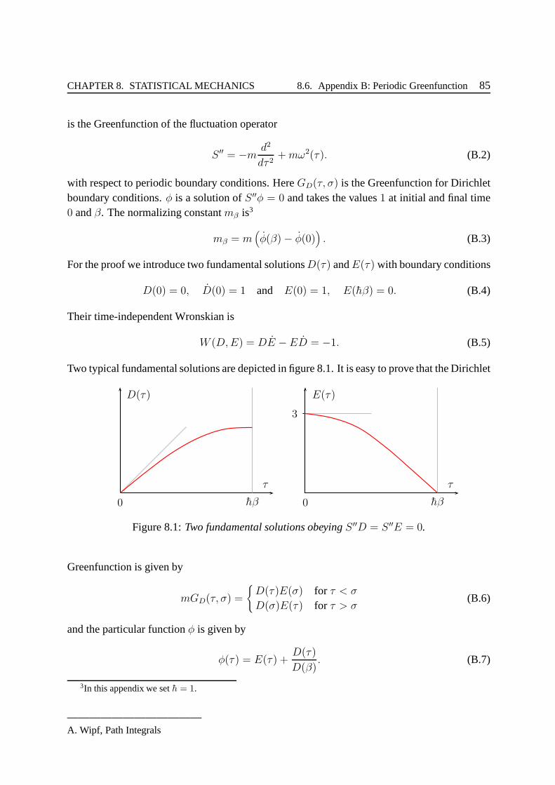
CHAPTER 8. STATISTICAL MECHANICS 8.6. Appendix B: PeriodicGreenfunction 85
is the Greenfunction of the fluctuation operator
S ′′ = −m d2
dτ 2+mω2(τ). (B.2)
with respect to periodic boundary conditions. HereGD(τ, σ) is the Greenfunction for Dirichletboundary conditions.φ is a solution ofS ′′φ = 0 and takes the values1 at initial and final time0 andβ. The normalizing constantmβ is3
mβ = m(
φ(β) − φ(0))
. (B.3)
For the proof we introduce two fundamental solutionsD(τ) andE(τ) with boundary conditions
D(0) = 0, D(0) = 1 and E(0) = 1, E(hβ) = 0. (B.4)
Their time-independent Wronskian is
W (D,E) = DE −ED = −1. (B.5)
Two typical fundamental solutions are depicted in figure 8.1. It is easy to prove that the Dirichlet
τ τ
3
0 hβ 0 hβ
D(τ) E(τ)
Figure 8.1:Two fundamental solutions obeyingS ′′D = S ′′E = 0.
Greenfunction is given by
mGD(τ, σ) =
D(τ)E(σ) for τ < σ
D(σ)E(τ) for τ > σ(B.6)
and the particular functionφ is given by
φ(τ) = E(τ) +D(τ)
D(β). (B.7)
3In this appendix we seth = 1.
————————————A. Wipf, Path Integrals

CHAPTER 8. STATISTICAL MECHANICS 8.6. Appendix B: PeriodicGreenfunction 86
We can make the following ansatz for the periodic Greenfunction,
GP (τ, σ) =α
mφ(τ)φ(σ) +GD(τ, σ). (B.8)
Clearly this function is symmetric in both arguments and hasthe valueα/m at initial and final(imaginary) time. The constantα is fixed by the periodicity condition
∂
∂τGP (τ, σ)|τ=0 =
∂
∂τGP (τ, σ)|τ=β
which implies
α
φ(0) − φ(β)
φ(σ) = m∂
∂τGD(τ, σ)|τ=β −m
∂
∂τGD(τ, σ)|τ=0. (B.9)
Inserting the Dirichlet Greenfunction (B.6) the right handside becomes
E(β)D(σ) − E(σ)) = −D(σ)
D(β)−E(σ) = −φ(σ), (B.10)
where we usedD(0) = 1 and that the Wronskian at final time isE(β)D(β) = −1. Comparingwith (B.9) we conclude thatα = −1 and this proves thatGP in (B.1) withmβ given in (B.3) isthe Greenfunction ofS ′′ with respect to periodic boundary conditions.
————————————A. Wipf, Path Integrals

Chapter 9
Monte Carlo Simulations
So far we have either dealt with exactly soluble systems likethe (time-dependent) oscillator orwith various expansions like the semiclassical, perturbative and high-temperature expansion. Inthis section I introduce a numerical method which plays an important role in modern develop-ments in (gauge-) field theories - theMonte-Carlo simulations.
One conveniently starts from the lattice approximation toZ(β, q) = K(hβ, q, q) in (6.21)for the density of the partition function. In the finite dimensional integral over the pointsw1, . . . , wn−1 defining the broken line path one setsw0 = wn = q and integrates overq toget the traceZ(β). More generally, the lattice approximation of expectationvalues reads
〈A〉 =
∫
dnwA(w) e−SE(w)
∫
dnwe−SE(w), where
∫
dnw =
∞∫
−∞
n∏
1
dwj, (9.1)
andSE(w) = SE(w1, . . . , wn) is the Euclidean lattice-action entering the discrete pathintegral(6.21). One could use standard numerical integration routines and approximate an integral by asum with a finite number of terms
∫
dnwf(w) ∼M∑
µ=1
f(wµ)∆wµ.
Note thatwµ denotes a configuration labelled byµ whereaswj denotes thej’th componentof the configurationw = (w1, . . . , wn). the If the space of integration is high-dimensional, itis however advantageous to choose the pointswµ at random instead of using a regular set ofpoints. Note, however, that the integrandexp(−S) will vary over many orders of magnitudefor different configurationswµ (we used that already in the semiclassical approximation).TheMonte Carlo method introduced by METROPOLIS, ROSENBLUTH, ROSENBLUTH and TELLER
is based on the idea ofimportant sampling[29]. Instead of selecting the pointswµ at randomthey are taken from that region where the dominant contributions to the integrals come from.More precisely, we choose the points according to the Boltzmann distribution
P (w) =1
Ze−SE(w), Z =
∫
e−SE(w) dnw (9.2)
87

CHAPTER 9. SIMULATIONS 9.1. Markov Processes and Stochastic Matrices 88
such that the Monte Carlo estimateA for the average ofA simply reduces to an arithmeticaverage
〈A〉 ∼ A =1
M
M∑
µ=1
A(wµ), (9.3)
whereM is the total number of points (states) generated in the MonteCarlo simulation.
9.1 Markov Processes and Stochastic Matrices
We now discuss a realization of important sampling. It is notquite straightforward, sincePis unknown. But it is possible to construct aMarkov processgenerating theM configurationswµ according to given transition probabilitiesW (wµ → wν) (the probability that the system,currently in configurationwµ makes a one-step transition into the configurationwν). Being atransition probability, the stochastic matrixW must be positive and normalized.
To proceed we consider a system with a finite numberf of degrees of freedom. We denotethe states bys ∈ 1, 2, . . . , f and the transition probabilities byW (s → s′) ≡ W (s, s′). Theyare positive,
W (s, s′) ≥ 0 (9.4)
and normalized∑
s′W (s, s′) = 1. (9.5)
A f -dimensional matrixW with these properties is calledstochastic matrix. In a two-stepprocess froms to s′ the system must pass through some intermediate states1 such that theprobability of a transition froms to s′ in two steps is given by
W (2)(s, s′) =∑
s1
W (s, s1)W (s1, s′). (9.6)
Similarly for ann-step process, we have
W n(s, s′) =∑
s1···sn−1
W (s, s1)W (s1, s2) · · ·W (sn−1, s′) =
∑
s1
W n−1(s, s1)W (s1, s′). (9.7)
Now one tries to construct a Markov process such that in the ’long-time’ limit n → ∞ theconfigurations are distributed according to (9.2). The ’long-time’ behavior of the system isdetermined by the limit ofW n asn→ ∞.
The set of stochastic matrices form a semigroup and every stochastic matrix transforms astochastic vector (af -dimensional vectorp with non-negative entriesPs obeying
∑Ps = 1)
into a stochastic vector. The entryPs of p is the probability to find the system in the states.
————————————A. Wipf, Path Integrals

CHAPTER 9. SIMULATIONS 9.1. Markov Processes and Stochastic Matrices 89
Consider for example a system with2 states and stochastic matrix
W =
(
a 1 − a
0 1
)
with W n =
(
an 1 − an
0 1
)
−→(
0 1
0 1
)
(9.8)
for a < 1. The stochastic matricesW n converges exponentially fast asn → ∞. Also note thatthis matrix has the eigenvalue1. Later we shall see that under certain assumptions onW theW n always converge to a stochastic matrix with identical rows.
A second and less trivial example is the stochastic matrix for a system with3 states,
W =
a 12(1 − a) 1
2(1 − a)
0 0 1
0 1 0
(9.9)
the powers of which are
W n =
an 12(1 − an) 1
2(1 − an)
0 1 0
0 0 1
for even n
and
W n =
an 12(1 − an) 1
2(1 − an)
0 0 1
0 1 0
for odd n,
and which again possesses the eigenvalue1. Fora < 1 a stochastic vectorp is mapped into
p −→ pW n −→(
0, p2 +p1
2, p3 +
p1
2
)
or(
0, p3 +p1
2, p2 +
p1
2
)
asn→ ∞, depending on whethern is even or odd. Note thatpW n approaches a periodic orbitexponentially fast and hence the Markov process does not converge. As we shall see, the reasonfor this lack of convergence is that the minima in all columnsof W are zero.
A stochastic matrix has always the eigenvalue1. The corresponding right-eigenvector is(1, 1, . . . , 1)T . To find the left-eigenvector we consider the sequence
pn =1
n
n−1∑
j=0
pW j. (9.10)
Since the set of stochastic vectors is compact this series must have a convergent subsequence
1
nk
nk−1∑
0
pW j −→ P .
————————————A. Wipf, Path Integrals

CHAPTER 9. SIMULATIONS 9.1. Markov Processes and Stochastic Matrices 90
We multiply withW from right and find
1
nk
nk∑
1
pW j −→ PW.
Subtracting the two series yields
1
nk(p− pW nk) −→ P −PW
Fornk → ∞ the left hand side tends to zero and hence
PW = P . (9.11)
and therefore any stochastic matrixW possesses at least one fixpointP that is a eigenvectorwith eigenvalue1. Let us now assume thatW possesses at least one column whose entriesare bigger or equal to a positive numberδ which means that all states have a non-vanishingprobability for a transition in a certain state. SuchW are calledattractive stochastic matrices.TheW in the first example above is attractive whereas the second one is not. For an attractiveW all statess have a non-vanishing probability to end up in a given states′, that isW (s, s′) > 0
for all s. Now we prove that an attractiveW is contractive on vectors of length2. First we notethat for two real numbersp andp′ we have
|p− p′| = p+ p′ − 2 min(p, p′),
such that for two stochastic vectors
‖p− p′ ‖ = 2 − 2∑
s
min(ps, p′s). (9.12)
Now we prove that an attractiveW is contractive on vectors∆ = (1, . . . ,f) with
‖∆‖ ≡∑
|s| = 2 and∑
s = 0. (9.13)
First we prove this statement for the difference of two cartesian basis vectorses, s = 1, . . . , f .For that we apply the identity (9.12) to the stochastic vectorsesW andes′W , that is to the rowss ands′ of W . For an attractiveW we find fors 6= s′
‖esW − es′W‖ = 2 − 2∑
s′′
min W (s, s′′),W (s′, s′′)
≤ 2 − 2δ = (1 − δ) ‖es − es′‖︸ ︷︷ ︸
=2
with 0 < δ < 1, (9.14)
and this proves thatW is contractive of the difference vectorses − es′. We used
mins′′
W (s, s′′)W (s′, s′′) ≥ min W (s, s∗)(W (s′, s∗) ≥ δ
————————————A. Wipf, Path Integrals

CHAPTER 9. SIMULATIONS 9.1. Markov Processes and Stochastic Matrices 91
wheres∗ belongs to the particular column ofW the elements of which are bigger or equal toδ.Now we prove the contraction property for all vectors∆ in (9.13). Since
∑
s:s≥0
s −∑
s:s<0
s = ‖∆‖ = 2
∑
s:s≥0
s +∑
s:s<0
s = 0
we conclude that
∑
s≥0
s = 1 and∑
s<0
s = −1. (9.15)
To simplify our notation we denote the non-negative elements of ∆ by s and the negativeelements bys′. Note that the index setss ands′ have no common elements. Because of(9.15) we have
‖∆‖ = 2 = −2∑
s
∑
s′ = −∑
ss′ ‖es − es′‖︸ ︷︷ ︸
=2
, (9.16)
where we assumeds 6= s′. To bound the norm of∆W we use
∑
ses = −∑
s′∑
ses ,∑
s′es′ = +∑
s
∑
s′es′,
where we made use of (9.15), and this leads to the inequality
‖∆W‖ = ‖∑
sesW +∑
s′es′W‖ = ‖ −∑
s′s(es − es′)W‖≤ −
∑
ss′‖(es − es′)W‖ ≤ −∑
ss′‖es − es′‖(1 − δ), (9.17)
where we used the inequality (9.14). Comparing with (9.16) leads to the inequality
‖∆W‖ ≤ (1 − δ)‖∆‖ (9.18)
which shows thatW is contractive on vectors of the form (9.13). Since this inequality is linear∆ we may drop the condition‖∆‖ = 2. HenceW is contractive on all vectors the elements ofwhich add up to zero and in particular on differences of two stochastic vectors.
Iterating the inequality we obtain
‖∆W n‖ ≤ (1 − δ)n‖∆ ‖. (9.19)
Now we apply this inequality top− P , whereP is the fixpoint in (9.11) andp is an arbitrarystochastic vector. Since the elements ofp−P add up to zero we conclude
‖(p−P)W n‖ = ‖pW n −P‖ n→∞−→ 0
————————————A. Wipf, Path Integrals

CHAPTER 9. SIMULATIONS 9.2. Detailed Balance, Metropolis Algorithm 92
or equivalently that
pW n n→∞−→ P . (9.20)
For the stochastic vectorses the left hand side is just the rows of the limit limW n = W eq
such thatW eq has identical rows. This means that all elements in a column of W eq are equal,similarly as in the example above.
W eq(s, s′) = limn→∞
W n(s, s′) = Ps′, (9.21)
wherePs′ is the elements′ of P . It follows that both the limit distributionP and matrixW eq
are unique. Else there would exist a second fixpointP ′ of the Markov process with
P ′s′ =
∑
s
P ′sW (s, s′) = lim
n→∞
∑
s
P ′sW
n(s, s′) =∑
s
P ′sPs′ = Ps′,
and this shows thatP is indeed the unique fixpoint.The generalization to systems with continuous degrees of freedom is clear. For the dis-
cretized path integral the states of a Markov process are thebroken line pathsw = (w1, . . . , wn)
on a time lattice withn sites. The probabilityPs becomes aprobability densityP (w). Sumsover the discrete indexs become integrals over the continuous variablesw1, . . . , wn. For thediscretized path integral the conditions (9.4) and (9.5) read
W (w,w′) ≥ 0 and∫
Dw′ W (w,w′) = 1. (9.22)
The fixpoint condition for the equilibrium distributionP (w) takes the form
P (w′) =∫
DwP (w)W (w,w′). (9.23)
In Euclidean Quantum Mechanics or in Quantum Statistics theequilibrium distributionP is thethe Boltzmann distribution, see (9.2).
9.2 Detailed Balance, Metropolis Algorithm
The interesting question is whether we can find a simple stochastic process which has the Boltz-mann distribution as its fixpoint. All processes used in actual simulations are constructed withstochastic matrices fulfilling thedetailed balancecondition
PsW (s, s′) = Ps′W (s′, s), (9.24)
which means that the transition froms to s′ is more probable as the inverse process if theequilibrium density is bigger ats′ than it is ats. If the detailed balance condition holds thenP
is indeed a fix point ofW since∑
s
PsW (s, s′) =∑
s
Ps′W (s′, s) = Ps′. (9.25)
————————————A. Wipf, Path Integrals

CHAPTER 9. SIMULATIONS 9.2. Detailed Balance, Metropolis Algorithm 93
The detailed balance condition does not fix the stochastic process uniquely. Considerationsof computational efficiency dictates its specific form. The local Metropolis-andheatbath al-gorithmare the most popular once since they can be applied to almost all statistical systems.More recently nonlocalcluster algorithmsare also used in cases where local algorithms faildue to ’critical slowing down’. Unfortunately cluster algorithms are not known for lattice gaugetheories.
In the METROPOLISalgorithm one starts with a certain initial configuration. The better theinitial configuration is chosen the less computer time is needed. For example, for a statistical lat-tice model at high temperature one should choose the variables at different lattice sites (havingthe lattice approximation (6.21) in mind) randomly, since there is almost no correlation betweenvariables at neighboring sites (see the high temperature expansion). If we are simulating a quan-tum mechanical system with a deep double well potential then(at low or zero temperature) onebetter chooses a initial configuration which resembles an instanton. After preparing the initialconfiguration one takes the ’first’ lattice variablew1 and changes it or leaves it according to thefollowing rules:
• First one replacesw1 tentatively by arandomlychosen trial-variablew′1.
• If S decreases (P increases) then the variable at site1 is set to the new valuew′1.
• If the action increases then a random numberr with uniform distribution between0 and1 is generated and the variable is changed tow′
1 only if exp(−∆S) > r. Otherwise thelattice variable retains its previous valuew1.
• The other sites of the lattice are then probed in exactly the same way.
• When one arrives at the last lattice site then one has completed oneMonte-Carlo sweep.
To test whether one is already near equilibrium one measuressome expectation values as afunction of iteration time. After the measured values have settled (that is we are not too far fromthe equilibrium distribution) then we may start ’measuring’ observables according to (9.3).
The Heat-bath algorithm is very similar as the Metropolis algorithm and I refer you to theliterature on Monte Carlo simulations for learning more about the various techniques to simulatequantum- or spin system. For an introduction into Monte Carlo (MC) methods, numericalstudies and further references I refer you to the nice paper of Creutz and Freedman [30], thetext book of NEWMAN and BARKENNA [31] or the text book of BERG [32].
9.2.1 Three-state system at finite temperature
Let us finally consider a physical system with 3 states.
H|n〉 = En|n〉 , n = 1, 2, 3 with E1 < E2 < E3. (9.26)
————————————A. Wipf, Path Integrals

CHAPTER 9. SIMULATIONS 9.2. Detailed Balance, Metropolis Algorithm 94
Since the energy decreases for the transitions|2〉 →|1〉 , |3〉 →|1〉 and|3〉 →|2〉 the correspond-ing transition amplitudes are constant in the Metropolis algorithm. The inverse transitions costenergy and the probabilities are proportional to the Boltzmann factors
bpq = eβ(Ep−Eq), p > q. (9.27)
We see that the Markov process has the stochastic matrix
W =1
2
2 − b21 − b31 b21 b311 1 − b32 b321 1 0
, (9.28)
and its powers converge to
W∞ =1
Z
e−βE1 e−βE2 e−βE3
e−βE1 e−βE2 e−βE3
e−βE1 e−βE2 e−βE3
, (9.29)
whereZ is the partition function,Z = exp(−βE1) + exp(−βE2) + exp(−βE3). Every initialprobability distribution converges to the Boltzmann distribution,
P =1
Z
(
e−βE1, e−βE2 , e−βE3
)
. (9.30)
The following figure shows the convergence to equilibrium for different initial distributions. Iused the differencesE2 − E1 = 0.5 andE3 −E2 = 0.3.
p1 p2 p3
W
p1 p2 p3
W
p1 p2 p3
W
p1 p2 p3
kalterStart
warmer Start
For a cold start with ground state as initial state and a hot start with equal probabilities for thedifferent states we find good convergence to equilibrium. Ifwe start with the most excited stateas initial state the the convergence is bad.
————————————A. Wipf, Path Integrals
Chapter 10
Berezin Integral
In any field theory describing the elementary particles in nature there are bosonicandfermionicfields. The latter describe the propagation of electrons, muons, neutrinos, quarks and so on. Inthis chapter we introduce anticommuting Grassmann-variables and the Berezin integral [33].These enter the path integral quantization of fermionic degrees of freedom.
10.1 Grassmann variables
So far we used the coordinate and momentum representations to formulate path integrals. Forwhat follows it is more convenient to use theFock-space representation, based on the creationand annihilation operators. In the particular case of the extensively discussed harmonic oscilla-tor these operators are related to the position and momentumoperators as follows,
a† =1√2h
(√ωmq − i√
ωmp
)
a =1√2h
(√ωmq +
i√ωm
p
)
, (10.1)
and they satisfy the commutation relation
[a, a†] = 1. (10.2)
The creation and annihilation operators are represented ontheanti-holomorphic functionsf(z)
endowed with the scalar product
(f1, f2) ≡1
2πi
∫
f1(z)f2(z)e−zz dzdz, z = x+ iy, dzdz = 2idxdy. (10.3)
The normalization is such that the constant functionf = 1 has unit norm. The creation- andannihilation operators are represented as
(af)(z) =∂
∂zf(z) and (a†f)(z) = zf(z). (10.4)
95

CHAPTER 10. BEREZIN INTEGRAL 10.1. Grassmann variables96
UsingH = hω(a†a + 1/2) and that the anti-holomorphic functionsfn(z) = (n!)−1/2zn forman orthonormal base in this space,
(fm, fn) =2
n!δmn
∫
e−r2
r2n+1dr = δmn, z = reiϕ,
we can calculate the matrix element〈z′|e−itH/h|z〉 of the evolution operator. One subtle pointin the bosonic case is thenormal ordering. One starts with the normal ordered Hamiltonian,that is the Hamiltonian with zero-point energy subtracted
:H: = H − 〈Ω|H|Ω〉 .
In order to replace the operators by classical variables,H(a†, a) → h(z, z), one needs to normalorder the evolution operator:e−itH/h: and not only the Hamiltonian. However, in the continuumlimit only the first order term1− iǫ:H(a†, a):/h in the series expansion for the normal orderedevolution operator contributes. But this term is assumed tobe already normally ordered.
Now we turn to the fermions, that is we replace (10.2) by
a, a† = 1 and (a†)2 = (a)2 = 0. (10.5)
These anti-commutation relations cannot be represented onfunctions of commuting variablesasz. But they can be represented on functions of anticommuting Grassmann-variablesα, α,
α, α = 0 and α2 = α2 = 0. (10.6)
As representation space we can choose theanalytic functionsdepending onα only. Sinceα2 = 0 such functions have a terminating series expansion
f(α) = f0 + f1α.
The Grassmann variables(α, α) generate theGrassmann algebra
G2 ≡ C ⊕ Λ1(V ) ⊕ Λ2(V )
and elements inG2 have the formf = f00+f10α+f01α+f11αα. More generally, forn degreesof freedom (10.6) generalizes to
αi, αj = αi, αj = αi, αj = 0, i, j = 1, 2, . . . , n. (10.7)
Grassmann variables are nilpotent,α2i = α2
i = 0, and they generate the Grassmann algebra
Gn ≡ ⊕Λk(V ), k = 1, 2, . . . , 2n,
whereΛ1(V ) = V has baseαi, αi and the elements
αi1 · · ·αipαj1 · · · αjq with p+ q = k and i1 < ... < ip, j1 < ... < jq
————————————A. Wipf, Path Integrals

CHAPTER 10. BEREZIN INTEGRAL 10.1. Grassmann variables97
form a basis ofΛk(V ). Actually Λk is isomorph to the exterior algebra ofk-forms on an2n-dimensional manifold.
Due to the anticommutation property there exist two types ofderivatives. Theleft derivativeand theright derivative. We shall always use the former. To compute the left-derivative ∂i of amonomial in the Grassmann variables one first bringsαi to the left (using the anti-commutationrules) and then drops this variable. For example,
∂i(αkαℓ) = δikαℓ − δiℓαk. (10.8)
Then the derivative is extended to polynomials and hence to all functions of the Grassmannvariablesαi, αi.
The fermionic creation and annihilation operators in (10.2) are represented by differentialoperators acting on analytic functionsf(α) = f(α1, . . . , αn) as follows,
(aif)(α) =∂
∂αif(α) and (a†if)(α) = αif(α) =⇒ [ai, a
†j] = δij1. (10.9)
We also would like to introduce ascalar producton the space of analytic functionsf(α). Forthat aim we introduce an integration over Grassmann variables. Such integrals have been intro-duced by Berezin and they are defined by the following linear functional [33, 34]:
∫
dαi αj =∫
dαiαj = δij and∫
dαi =∫
dαi = 0. (10.10)
To integrate a monomial with respect toαi one first bringsαi in the monomial to the left (usingthe anti-commutation rules) and then drops this variable. For example,
∫
dαi αjαk = δijαk − δikαj, (10.11)
and similarly for higher monomials. We see that the Berezin integral∫
dαi is equivalent to leftderivative with respect to∂αi
. For the integral overall Grassmann variableswe choose the signconvention such that
∫
DαDαn∏
1
(αiαi) = 1, where DαDα ∝n∏
1
dαin∏
1
dαi, (10.12)
and it is supposed that thedαi anddαj anticommute with each other and withαi andαj . Theintegral over Grassmann variables which are permutations of theα’s andα’s in (10.12) is thengiven by the anti-commutation rules. The integral of less then2n variables is always zero,
∫
DαDαp∏
1
αi
q∏
1
αj = 0 for p+ q < 2n. (10.13)
From this property it follows that under a shift of the integration variables by Grassmann vari-ables the Berezin integral is not changed,
∫
DαDα f(α + η, α+ η) =∫
DαDα f(α, α). (10.14)
————————————A. Wipf, Path Integrals

CHAPTER 10. BEREZIN INTEGRAL 10.1. Grassmann variables98
Actually, to prove this translational invariance one also uses(α + η)2 = αη + ηα = 0. Let usnow see how the Berezin integral changes under linear transformations
βi =∑
j
Uijαj and βi =∑
j
Vijαj (10.15)
of the integration variables in (10.12). One finds∫
DαDαn∏
1
(βiβi) =∑
ji,kℓ
∏
i,ℓ
UijiVℓkℓ
∫
DαDα (αjiαkℓ).
Note that only those terms contribute for whichj1, . . . , jn andk1, . . . , kn are permutationsof 1, . . . , n. These permutations are denoted byσ andσ. Thus we find
∫
. . . =∑
σ,σ
∏
i,ℓ
Uiσ(i)Vℓσ(ℓ) sgn(σ)sgn(σ) = detU · detV. (10.16)
For theories containing fermions the Gaussian Berezin integrals are as important as the ordinaryGaussian integrals are for theories containing bosons. With the help of (10.16) it is not difficultto compute the Gaussian integral
Z =∫
DαDα e−αAα, where αAα = αiAijαj. (10.17)
One just changes variables according toβi = Aijαj (and leaves theα’s) so that
Z =∫
DαDα e−αiβi =1
n!
∫
DαDα (βiαi)n =
∫
DαDα∏
(βiαi) = det(A).
We end up with the important formula∫
DαDα e−αAα = det(A), αAα = αiAijαj. (10.18)
This should be compared with the corresponding bosonic Gaussian integral for which one ob-tains the inverse square root of the determinant ofA.
Thegenerating functionfor Grassmann integrals can be computed by shifting the integrationvariables in (10.18) according to
α −→ α−A−1η and α −→ α− ηA−1.
Using the translational invariance of the Berezin integral, see (10.14), one arrives at∫
DαDα e−αAα+ηα+αη = det(A) eηA−1η, ηα = ηiαi. (10.19)
Now we define thescalar productof two analytic (inα) functions, similarly as in the bosoniccase, according to
(g, f) =∫
DαDα g†(α)f(α)e−αα, (10.20)
————————————A. Wipf, Path Integrals

CHAPTER 10. BEREZIN INTEGRAL 10.1. Grassmann variables99
where the adjoint of a functiong = g0 + giαi + gijαiαj + . . . is given byg† = g0 + giαi +
gijαjαi + . . .. Inserting the expansions forg† andf yields
(g, f) =n∑
p=0
gi1...ipfi1...ip (10.21)
for the scalar product of two functionsg(α) andf(α). The last formula makes clear that thescalar product is indeed sesqui-linear and positive as required. The space of analytic functionsf(α), endowed with this scalar product, forms the Hilbert space on which the linear operatorsare represented. One can show that the operatorsa anda† are (formally) adjoint of each otheron this Hilbert space. A basis of the Hilbert space is defined by the orthonormal set of Fockstates
∏a†i |0〉, where|0〉 is represented by the constant function1.
Returning ton = 2 we consider a generalnormal orderedlinear operatorA = :A:,
A = K00 +K01a+K10a† +K11a
†a
= K00 +K01∂
∂α+K10 α +K11 α
∂
∂α. (10.22)
Applying this operator to an element of the Hilbertspacef(α) = f0 + f1α we obtain
(Af)(α) = K00(f0 + f1α) +K01f1 +K10f0α+K11f1α
=∫
A(α, β)e−ββf(β)dβdβ. (10.23)
where the kernel on the right hand side is given by
A(α, β) = eαβAN(α, β) with AN (α, β) = K00 +K01β +K10α +K11αβ.
This generalizes in an obvious way to more than one degree of freedom: a normally orderedlinear operatorA has a kernelA which is obtained fromA by replacinga, a† by β, α andmultiplying the resulting expression withexp(αβ). Similarly one can show that
(AB)(α, α) =∫
A(α, β)B(β, α)e−ββdβdβ.
With these formulas we can now derive the path integral representation for thekernelof thenormal ordered evolution operatorK(t, a, a†). As in the bosonic case we divide the time interval[0, t] into n time steps of equal lengthǫ = t/n and obtain for the kernel
K(t, αn, α0) =∫ n−1∏
i=1
dαidαin∏
i=1
KNǫ (αi, αi−1) exp
(
−n−1∑
1
αiαi +n∑
i=1
αiαi−1
)
, (10.24)
where the variablesα0 and αn at initial and final time are held fixed. In the continuum limitn→ ∞ or ǫ→ 0 we may approximate
KNǫ (α, α) ∼ exp
(
−iǫhHN(α, α)
)
————————————A. Wipf, Path Integrals
CHAPTER 10. BEREZIN INTEGRAL 10.1. Grassmann variables100
and thus we can rewrite (10.24) as follows
K(t, αn, α0) = limn→∞
∫
DαDα exp
(
αnαn +n∑
i=1
[
αi(αi−1 − αi) − iǫHN (αi, αi−1)])
= limn→∞
∫
DαDα exp
(
α0α0 +n−1∑
i=0
[
(αi+1 − αi)αi − iǫHN (αi+1, αi)])
,
where one integrates over the Grassmann variablesαi, αi with i = 1, 2, .., n− 1. The secondform follows from the first by a ’partial integration’ and shows, that the factorsαnαn andα0α0
are surface terms which can be neglected in the continuum limit. Thus in the continuum limitwe end up with the following path integral
K(t, αn, α0) =
α(t2)=αn∫
α(0)=α0
DαDα exp
−t2∫
t1
dt[
αα + iHN(α, α)]
. (10.25)
Note that the function in the exponent is just the action corresponding to the (normal ordered)HamiltonianH. This means that the path integral for fermionic degrees of freedom is formallythe same as for bosonic systems. The crucial difference (which forbids a probabilistic interpre-tation) is the replacement ofc-numbers by ’Grassmann numbers’. Before turning to the field-theoretical generalization we discuss an interesting application of (10.25) to supersymmetricquantum mechanics.
————————————A. Wipf, Path Integrals

Chapter 11
Supersymmetric Quantum Mechanics
In this section we examine simple1 + 0-dimensional supersymmetric field theories. In1 + 0
dimensions the Poisson-algebra reduces to time translations generated by the HamiltonianHand the hermitian field and momentum operatorsφ(t) andπ(t) may be viewed as position andmomentum operators of a point particle on the real line in theHeisenberg-picture. Hence susyfield theories in1+0 dimensions are particular quantum mechanical systems [35]. Such systemsare interesting in their own right since they describe the infrared-dynamics of supersymmetricfield theories in finite volumes. In mathematical physics supersymmetric QM has been usefulin proving index theorems for physically relevant differential operators [36]. There exist severalextensive texts on susy quantum mechanics [37, 38, 39] in which the one-dimensional systemsare discussed in detail. First we consider the simple Hamiltonian
H = HB +HF , where HB = ωa†a, HF = ωb†b, (11.1)
anda andb are bosonic and fermionic annihilation operators:[a, a†] = 1 andb, b† = 1. TheFockspaceis generated by acting with the creation operators on the vacuum defined by
a|0〉 = b|0〉 = 0. (11.2)
Using the commutation and anticommutation relations for the creation and annihilation oper-ators one finds that besides the non-degenerate zero-energyground state all excited states aredouble degeneratesince(a†)n|0〉 andb†(a†)n−1|0〉 have both energyE = nω. Introducing thefermion number operatorNF = b†b we see that there is always a bosonic state (NF = 0) anda fermionic one (NF = 1) with the same energy. This system is the simplest supersymmetricquantum mechanical system, namely thesupersymmetric harmonic oscillator(we have set themass to one and shall also seth = 1 in what follows).
Let us now generalize the above Hamiltonian and consider
H = HB +HF , where HB =1
2
(
p2 +W 2)
and HF = W ′b†b, (11.3)
101
CHAPTER 11. SUPERSYMMETRIC QUANTUM MECHANICS 102
whereW (x) is an arbitrary function. Using the formula (10.25) and the corresponding bosonicresult (2.32) yields the following path integral representation for the evolution kernel
K(t, q, q′, α, α′) =∫
DwDαDα eiS[w,α,α], (11.4)
where one sums over all pathsw(t), α(t), α(t) with
w(0) = q′, w(t) = q, α(0) = α′ and α(t) = α.
The action contains the familiar bosonic partSB and an additional term depending on the Grass-mann values path,
S =∫
dtL = SB[w] + SF [w, α],
with Lagrangian density
L =1
2w2 − 1
2W 2(w) + iαα−W ′(w)αα. (11.5)
This models are supersymmetric. Under a supersymmetry transformation
δw = ǫα + αǫ, δα = −(iw +W )ǫ δα = −ǫ(−iw +W ) (11.6)
with constant anticommuting parametersǫ, ǫ, the variation of the Lagrange function is a totaltime-derivative,
δL =d
dt
(
wαǫ− iW ǫα)
(11.7)
and thus the action is invariant.It has been observed by Nicolai [40] that the following transformation of the bosonic field
w(t) −→ y(t) = w(t) + iW (w(t)) (11.8)
for which
1
2y2 =
1
2w2 − 1
2W 2 + iWw and
δy(t)
δw(t′)=
(
d
dt+ iW ′
)
δ(t− t′) (11.9)
simplifies the analysis considerable, due to supersymmetry. To see that we first note that
Dw∫
DαDα e−(αα+iW ′αα) = Dw det
(
d
dt+ iW ′
)
= Dy, (11.10)
which means that the Jacobian of the bosonic transformationis canceled by the fermionic inte-gral. We have been a bit sloppy with the boundary conditions,for a more detailed analysis ofthis point I refer you to the paper of Ezawa and Klauder [41]. Second we observe that
1
2
∫
y2dt =1
2
∫ (
w2 −W 2)
dt+ i∫
Wwdt = SB + i∫ q
q′W (w)dw. (11.11)
————————————A. Wipf, Path Integrals
CHAPTER 11. SUPERSYMMETRIC QUANTUM MECHANICS 103
Inserting the last two identities into the evolution kernel(11.4) we see that this kernel is givenby a Gaussian integral in terms of the new variables,
K(t, . . .) = exp(∫ q
q′W) ∫
Dy eiy2/2. (11.12)
To obtain the partition function we continue to imaginary time t = −iτ such that the actionchanges into the Euclidean action
SE =∫
dτL with L =1
2w2 +
1
2W 2 + αα +W ′αα, (11.13)
and the supersymmetric transformations are modified to
δα = (w −W )ǫ δα = ǫ(−w −W ) with δL =d
dτ(wαǫ− ǫαW ) . (11.14)
Note that the transformation ofw is unchanged. TheNicolai mapof the Euclidean model reads
w(τ) −→ y(τ) = w(τ) +W (w(τ)). (11.15)
To obtain the ’partition function’ one integrates overβ-periodic pathsw(τ) andβ-antiperiodicpathsα(τ), α(τ) (see below). Such finite temperature boundary conditions break supersymme-try which transforms periodic bosonic fields into periodic fermionic fields. Physically this isnot surprising since a equilibrium state is not invariant under Lorentz transformation and hencecannot be supersymmetric. After all, supersymmetry is an extension of Lorentzsymmetry. If weinstead integrate only over periodic paths then supersymmetry is not violated by the boundarycondition. This corresponds to the Euclidean model and forβ → ∞ expectation values becomevacuum expectation values. For periodic boundary conditions we can transform to Nicolai vari-ables and obtain
Zper =∮
Dy e−y2/2, (11.16)
where one integrates overβ-periodic pathsy(τ). When treating the boundary conditions morecarefully one can indeed show that for matrix elements the cancellation between the fermionicdeterminant and the bosonic Jacobian occurs for a certain definition of the fermionic path inte-gral and thus the above formal manipulations are justified.
Note that the correlation functions can now be evaluated as
〈w(τ1) . . . w(τn)〉 =∫
w(τ1) . . . w(τn)dµ0(y)
with the Gaussian measure as in (11.16) rather than with the complicated interaction measure.However, the moments are not that easy to calculate becausew(t) is generally a nonlinear andnonlocal function of the fluctuatingy-path as determined by the inverse Nicolai map.
————————————A. Wipf, Path Integrals

Chapter 12
Path Integral for Fermion Fields
After introducing path integrals in quantum mechanics we now turn to the path integral rep-resentation of field theories. In this chapter we discuss thefermionic sector of theSchwingermodel, which is probably the simplest non-trivial field theory. The Schwinger model is justQED for massless fermions in 2 dimensions [42]. This model showsat least two (related)striking features. First the classically massless ’photon’ acquires a mass due to its interactionwith the massless fermions and second the operatorψ(x)ψ(x) has a non-vanishing vacuumexpectation [43]. Clearly, since this model contains fermions we first must discuss the pathintegral for fermionic, and in particular the path integralrepresentation of then-point functions.
The zero-temperature Schwinger model has been solved some time ago by using operatormethods [44] and more recently in the path integral formulation [45]. Some properties of themodel (e.g. the non-trivial vacuum structure) are more transparent in the operator approachand others (e.g. the role of the chiral anomaly) are better seen in the path integral approach.More recently the Schwinger model has been solved in the pathintegral approach on the 2-dimensional sphere and the role of the fermionic zero modes has been emphasized [46].
12.1 Dirac fermions
To arrive at the path integral for Dirac fermions (e.g. electrons). we generalize the above resultsto field theory, that is, we replace
αi(t) → ψ(x , t) and αi(t) → ψ(x , t).
The discrete indexi becomes the continuous position in space and the summation is to bereplaced by an integration over space.
For the Dirac fermions minimally coupled to a gaute fieldAµ the action reads
S =∫
ΩL with L = ψ(i /D −m)ψ. (12.1)
104
CHAPTER 12. FERMION FIELDS 12.1. Dirac fermions105
The canonical momentum density is proportional to the field,
π =δLδψ
= iψγ0 = iψ†, (12.2)
and not to the time-derivative of the field, since the Lagrangian density only contains first orderderivatives. The Hamiltonian is given by a Legendre transform,
H =∫
H, H = πψ − L = −iψγjDjψ +mψψ. (12.3)
Inserting this into the field-theoretical generalization of (10.25) we obtain the functional integralrepresentation
Z =∫
DψDψ eiS[ψ,ψ], (12.4)
whereS is the action for fields on a space-time regionΩ. The boundary conditions for the fieldson the boundary∂Ω must be specified. Here we choose forΩ the Minkowski space to avoidboundary effects.
We are primarily interested in the generating functional inthe presence of external currents,which now is constructed by using twoanticommuting sourcesη(x) andη(x):
Z[η, η] =∫
DψDψ exp(
iS[ψ, ψ] + i∫
[η(x)ψ(x) + ψ(x)η(x)]ddx)
. (12.5)
We can simplify this path integral by expanding the exponentabout its extremum. The exponentis extreme for
ψcl = −(i /D −m)−1η and ψcl = −η(i /D −m)−1.
Shifting the variables according toψ → ψcl + ψ etc. the exponent becomes
iScl + iS[ψ, ψ], where Scl = −η 1
i /D −mη = −
∫
η(x)GF (x, y)η(y), (12.6)
andGF denotes the Feynman propagator
(i /Dx −m)GF (x, y) = δ(x− y). (12.7)
For example, for the free field (A = 0) one has
GF (ξ) = −(i/∂ +m)∆F (ξ), (12.8)
where∆F is the Feynman propagator of the Klein-Gordon field:
∆F (ξ) = − 1
(4π)2
∫
d4xe−ipξ1
p2 −m2 + iǫ=⇒ (∂µ∂
µ +m2)∆F = δ4(ξ). (12.9)
————————————A. Wipf, Path Integrals
CHAPTER 12. FERMION FIELDS 12.1. Dirac fermions106
SinceScl is independent of the integration variables, the path integral (12.5) reads
Z[η, η] = det(i /D −m) exp(
− i∫
η(x)GF (x, y)η(y)ddxddy)
. (12.10)
Differentiating (12.5) with respect to the sourcesη andη yields the correlation function
T 〈0|ψα1(x1)ψβ1(y1)...ψαn(xn)ψβn(yn)|0〉
=1
Z[0]
δ2n
δηβn(yn)δηαn(xn)...δβ1η(y1)δηα1(x1)Z[η, η]|η=η=0. (12.11)
The n-point functions, for n odd, vanish since the source term is even in the current. In particu-lar, forn = 2 we recover the propagator (Feynman propagator). Using Wick’s theorem (whichwe shall proof later) one shows that the2n-point function can be expressed in terms of the twopoint function only. This shows already the equivalence of the Berezin path integral approachand the canonical approach.
We conclude this section with the proof of Wick’s theorem forfermions. This theorem isextensively used in quantum field theory. Originally it was proven using canonical methods.Now we shall see how to derive this theorem using functional integration. What we show is thefollowing representation for the2n-point function in terms of the2-point function:
T 〈0|ψ(x1)ψ(y1)...ψ(xn)ψ(yn)|0〉 =1
Z[0]
∫
DψDψ ψ(x1)ψ(y1)...ψ(xn)ψ(yn)eiS[ψ,ψ]
= (−i)n∑
π∈Sn
sign(π)n∏
j=1
GF (xj , yπ(j)). (12.12)
To prove this identity we use the generating functional (12.5) and expand the exponent contain-ing the source-terms in a power series:
Z[η, η] =∫
DψDψ eiS∑
n
i2n
(2n)!
∫
dx1...dx2n
2n∏
i=1
(η(xi)ψ(xi) + ψ(xi)η(xi))
=∑
n
(−)n
(2n)!
∫ 2n∏
1
dxiηα1(x1)...η
βn(x2n)(2n)!
n!n!
∫
DψDψ eiSψα1(x1)...ψβn(x2n),(12.13)
where we have used the anticommutation properties of the fields and sources and the fact thatthe functional integral is nonzero only if there are as many fields as adjoint fields. On the otherhand using (12.10) we may expand the generating functional as
Z[η, η]
Z[0]=∑
n
(−i)nn!
∫
dx1...dxndy1...dynη(x1)η(y1)...η(yn)n∏
i=1
GF (xi, yi) (12.14)
and using again the anticommutation properties we can rewriteZ as
Z[η, η]
Z[0]=∑
n
(−i)nn!n!
∫ n∏
1
dxidyiη(x1)η(y1)...η(yn)∑
π∈Sn
n∏
i=1
sign(π)GF (x2, yπ(i)). (12.15)
————————————A. Wipf, Path Integrals
CHAPTER 12. FERMION FIELDS 12.1. Dirac fermions107
Comparing with (12.13) and using the fact that the sources are arbitrary, proves the Wick theo-rem (12.12).
Finally we turn to the fermionic thermal Green’s functions.As we have already seen in inquantum mechanics, the transition to the Euclidean sector is made by replacingt → −iτ suchthat
∂0 → i∂0, A0 → iA0, A0 → −iA0, γ0 → iγ0, γ0 → −iγ0 (12.16)
(and keeping the other quantities fixed) or equivalently by replacingxj → ixj such that
∂j → −i∂j , Aj → −iAj , Aj → iAj , γj → −iγj , γj → iγj . (12.17)
Since we prefer to use a Minkowskian metric with signature(+,−,−,−) we continue accord-ing to (12.17) rather than (12.16). In the case of Dirac fermions the exponent in (12.5) becomesthen
iS + i∫
(ηψ + ψη) −→ −SE +∫
(ηψ + ψη),
SE =∫
LE, LE = −iψ /Dψ +mψψ. (12.18)
When calculating the partition functionZ(β) at finite temperature we must choose antiperiodicboundary conditions for the fields, in contrast to to the bosonic case (see (8.22)). The reason isthat the fermionic Green’s functions areβ-periodic in imaginary time [48]. This is taken intoaccount if antiperiodic boundary conditions in the path integral are chosen and then the partitionfunction becomes
Z(β) = const·∫
a.p.
DψDψ e−SE [ψ,ψ], (12.19)
wherea.p. should indicate that we integrate over anti-periodic fieldsψ(hβ, x ) = −ψ(0, x ) andanalog forψ. In analogy to (12.5) the generating functional for the thermal Green’s functionsreads
Z[β, η, η] =∫
a.p.
DψDψ exp(
− S[ψ, ψ] +
βh∫
0
ddx [η(x)ψ(x) + ψ(x)η(x)])
(12.20)
and the thermal correlation functions are obtained by differentiation with respect to the externalcurrent
T 〈0|ψα1(x1)ψβ1(y1)...ψβn(yn)|0〉β =(−)n
Z[0]
δ2n
δηβn(yn)...δα1 η(x1)Z[η, η]|η=η=0 (12.21)
whereT denotes the Euclidean time ordering. Note the presence of the factor(−1)n in contrastto (12.11). This is due to the Wick rotation to imaginary time.
————————————A. Wipf, Path Integrals

CHAPTER 12. FERMION FIELDS 12.2. The index theorem for the Dirac operator 108
Next we simplify (12.21). We could calculate a ’classical’ path with antiperiodic boundaryconditions, calculate the partition kernel and then integrate over the boundary conditions. Thisapproach analogous to is rather involved in the present situation. Therefore we choose a some-what different (and more formal) approach which can be applied for quadratic actions (and forsimple boundary conditions). We just apply the Gauss integral formula to (12.20)
Z[β, η, η] = det(i /D −m) e−(η(x),Gβ(x,y)η(y)), Gβ(x, y) = 〈x| 1
i /D −m|y〉. (12.22)
Gβ(x, y) is the thermal Green’s function of(i /D−m) (that is the Green’s function on the spaceof the functions antiperiodic inβ). The formula (12.22) then implies in particular
T 〈ψ(x)ψ(y)〉β = − 1
Z[β, 0]
δ2
δη(y)δη(x)Z[β, η, η]|η=η=0 = Gβ(x, y). (12.23)
More generally, the Wick-theorem (12.12) still holds if we drop the(−i)n and replace theFeynman propagator by the thermal Green’s function (or Euclidean propagator) on the righthand side of (12.12). This concludes our proof of the equivalence between the functional inte-gral approach and the canonical approach for fermionic systems. We have seen that formallythere is a close analogy of fermionic path integrals with those in quantum mechanics. So farwe haven’t dealt with the inherent divergences of field theories, a feature with is not presentin ordinary quantum mechanics. Finally we have seen the pathintegral formalism allows for aunified treatment of zero-temperature and finite temperature systems.
12.2 The index theorem for the Dirac operator
When solving the (Euclidean) Schwinger model we must calculate the partitionZ in (12.19) orequivalently its logarithm, the effective action
Γ = logZ = log det /D (12.24)
(see (12.22)), where we assume the fermions to be massless. As we shall see later, this deter-minant can be calculated explicitly in2 dimensions by integrating the chiral anomaly. As a firststep we now determine the number of zero modes of/D. It will turn out that this number is aphysically and mathematically interesting number.
We use the notation and convention as in (8.67-8.70) and assume that space-time is evendimensional so that we can introduceγ5 = (−i)n(n−1)/2γ1γ1 · · ·γn (the factor is chosen suchthatγ2
5 = Id) which anti-commutes with allγ’s
γ5, γµ = 0 =⇒ γ5, /D = [γ5, /D
2] = 0. (12.25)
————————————A. Wipf, Path Integrals

CHAPTER 12. FERMION FIELDS 12.2. The index theorem for the Dirac operator 109
In Euclidean space-time we may takeγ1, . . . , γn to be hermitean so thati /D is selfadjoint andwe shall assume that its spectrum is discrete. Sinceγ5 anticommutes with the Dirac operator all’excited’ eigenfunction of/D come in pairs,
i /Dχ = 〈χ =⇒ i /D(γ5χ) = −γ5(i /Dχ) = −〈(γ5χ) (12.26)
i.e. theγ5-transform of an eigenmode has the opposite eigenvalue (note thatγ5χ has the samenorm asχ and hence cannot be zero). This implies that all excited states of− /D
2are (at least)
double degenerate, more precisely to each left-handed eigenmodeγ5ψL = ψL there is a right-handed partnerγ5ψR = −ψR with the same eigenvalueE = λ2. In terms of the eigenfunctionsof i /D they readψL = 1
2(1 + γ5)χ andψR = 1
2(1 − γ5)χ. This pairing need not and generally
does not occur for the zero-energy states. The ground statesof − /D2
are also eigenstates ofi /Dwith eigenvalue zero (this is not true for the excited states) and thus have fixed chirality. Nowwe define the index of the Dirac operator as the number of left-handed minus the number ofright-handed zero modes of− /D
2or i /D:
index(i /D) = n+ − n−. (12.27)
This index can be computed quite differently. For that we note that the (super) trace trγ5 exp(β /D2)
can be computed via path integrals similarly to the partition function in (8.3) and (8.4). Usingthe eigenfunction of− /D
2in evaluating the trace we find
tr γ5eβ /D
2
=∑
n
(
e−βEL,n − e−βER,n
)
= n+ − n− = index(i /D), (12.28)
where we have used that due to the pairing of the excited states only the zero-modes contributeto the sum. Note in particular that the super-trace isβ-independent.
The supertrace can now be calculated by using the density (8.65) of the partition function.This way we find for the index
n+ − n− = tr γ5eβ /D
2
=∫
dnx tr(
γ5Z(β, x))
(12.29)
where the last trace is over spin- and internal color indicesandZ(β, x) possesses the pathintegral representation (8.74). Since the super-trace is independent ofβ we may assumeβ to bevery small and use the high temperature expansion (8.78).
In two dimensionsΣF = γ5F01 and we find∫
tr γ5Z(β, x) =1
4π
∫
tr (γ25)F01 +O(β). (12.30)
With our sign convention forγ5 we obtain in four dimensions tr(γ5ΣµνΣαβ) = ǫµναβ and thus
∫
tr γ5Z(β, x) =1
(4π)2
∫1
2ǫµναβFµνFαβ +O(β). (12.31)
————————————A. Wipf, Path Integrals

CHAPTER 12. FERMION FIELDS 12.3. The Schwinger model, Part I110
The higher orders inβ must be identically zero and we conclude
index(i /D) =1
2π
∫
d2xtrF01 n = 2 (12.32)
and
index(i /D) =1
32π2
∫
d4xǫµναβ tr (FµνFαβ) =1
16π2tr F ∗F n = 4. (12.33)
These identities and their analog in higher dimensions relate the index ofi /D to certain flux-integrals (Chern-densities). In particular we conclude that these fluxes are always integers, atleast if the spectrum of the Dirac operator is discrete. The spectrum is certainly discrete if theEuclidean space-time is bounded, for example a sphere or a torus. On unbounded spaces orspaces with boundaries the index-theorem is modified [49] (since the fluxes are not integers ingeneral).
12.3 The Schwinger model, Part I
As already mentioned earlier, the Schwinger model [42] is Quantum-electrodynamics for mass-less fermions in 2 dimensions and the corresponding action contains the fermion field coupled tothe electromagnetic field, that is (12.18) with a vanishing mass, and the addition of the Maxwellterm for the ’photons’:
S[A, ψ, ψ] =∫
LF + LB, LF = −iψ /Dψ, LB =1
4FµνF
µν + Lgf , (12.34)
whereLgf are gauge terms due to the gauge fixing procedure (see below).We solve theSchwinger model at zero temperature, so that the integrals in (12.34) are over the whole Eu-clidean plane. The (Euclidean) generating functional may also contain a source term for theelectromagnetic field, so that
Z[J, η, η] =∫
DADψDψ exp(
− S[A, ψ, ψ] +∫
d2x [AµJµ + ηψ + ψη]
)
(12.35)
In a first step we treat the fermionic part of the path integralonly and thus may assume thephoton field to be an external field. Integrating out the fermionic degrees of freedom accordingto (12.22) yields
Z[J, η, η] =∫
DA det(i /DA)e−∫
LB+i∫η(x)G(x,y)η(y)+
∫AµJµ
. (12.36)
The reason which allows the model to be solved exactly is thatthe electron propagator and thefermionic determinant in an arbitrary external field can be found explicitly, as has been observedby Schwinger. For that purpose we introduce
Φ =1
∆
(
∂αAα + iΣαβFαβ
)
(12.37)
————————————A. Wipf, Path Integrals

CHAPTER 12. FERMION FIELDS 12.3. The Schwinger model, Part I111
where the matricesΣαβ have been introduced in (8.71). Note that under a gauge transformationA→ A+ dΛ this functions transforms asΦ → Φ + Λ. Using the identity2iΣαβ = γαγβ − δαβ
one sees that
/∂Φ =1
∆
(
γµγαγβ∂µ∂αAβ)
=1
∆γβ∆Aβ = γβAβ. (12.38)
In particular in2 dimensionsΣF = γ5F01 and
Φ =1
∆
(
∂A + iγ5F01
)
. (12.39)
Taking into account thatγ5 anti-commutes with the Dirac operator we can rewrite the Diracoperator as
/D = /∂ − iγµAµ = /∂ − i/∂Φ = eiΦ†/∂e−iΦ. (12.40)
Note, that the last identity holds only in2 dimensions since we have used thatγµΦ = Φ†γµ.Now it is clear that the exact propagator which obeys the equation
i /DG(x, y, A) = δ2(x− y) (12.41)
has the form
G(x, y, A) = eiΦ(x)G0(x− y)e−iΦ†(y) (12.42)
whereG0 denotes the free massless propagator
G0(ξ) = −i/∂∆0(ξ) where ∆0(ξ) = − 1
4πlog(µ2ξ2). (12.43)
(µ is an infrared cut-off which could be left out if we would quantize the model on a finiteregion instead ofR2).
To compute the fermionic determinant in (12.36) we employ the zeta-function method. Weformally definedet(i /D) as the square root ofdet(− /D
2). From and (6.93) and (6.94) we see
that
ζ− /D2(s) =
1
Γ(s)
∫
dtts−1tr et /D2
(12.44)
and
log det(i /D) =1
2log det(− /D
2) = −1
2
d
dsζ− /D
2(s)|s=0. (12.45)
Let us now define a one parametric family of Dirac operators which interpolates between/D and/∂, namely
/Dα = eiαΦ†/∂e−iαΦ, (12.46)
————————————A. Wipf, Path Integrals
CHAPTER 12. FERMION FIELDS 12.3. The Schwinger model, Part I112
such that
δ /Dα = i(Φ† /Dα − /DαΦ). (12.47)
The variation of the zeta-function becomes then (we suppress the indexα)
δζ− /D
2(s) =1
Γ(s)
∫
ts−1tr et /D2
t(δ /D /D + /D δ /D) =2i
Γ(s)
∫
tstr et /D2
/D2(Φ† − Φ)
=4
Γ(s)
∫
tstr et /D2
/D2γ5
1
∆F01 = − 4s
Γ(s)
∫
ts−1tr et /D2
γ51
∆F01,
where we have partially integrated to obtain the last equality. Since finallys → 0 only thesingular part (more precisely the single pole ats = 0) of the integral survives, because of thefactor s. We may split the integration overt into an integration from0 to ǫ and fromǫ to ∞.The second integral is finite fors = 0 (recall that the free heat kernel falls off liket−1) and weneed only consider the interval near0. Here we may use the asymptotic expansion (8.78) forthe heat kernel of/D
2α and find (Fα = αF ):
δζ− /D
2(s) = − s
πΓ(s)
ǫ∫
0
dt[ts−2tr (γ51
∆F01) + ts−1αtr (γ5F01γ5
1
∆F01) +O(ts)
]
. (12.48)
Since the first term in (12.39) vanishes the integration overt yields
− 2α
πΓ(s)ǫs(
F011
∆F01 +O(s)
)
.
Finally, sinceΓ(s) ∼ 1/s for s→ 0 thes-derivative in (12.45) yields
d
dαlog det(i /D) =
α
πtr(
F011
∆F01
)
. (12.49)
Integratingα from 0 to 1 yields
log det(i /D) − log det(i/∂) =e2
2π
∫
F011
∆F01 = − e2
2π
∫
Aµ(δµν − ∂µ∂ν
∆)Aν , (12.50)
where we have reinserted the electric chargee. In what follows we may drop the (divergent) de-terminant of the free Dirac operator, since it is independent of the gauge potential and chancelsin expectation values. Hence the effective action in (12.36) entering the integration over theremaining ’photon’-field is
Γ[A] =1
4
∫
FµνFµν +
e2
2π
∫
Aµ(δµν −∂µ∂ν
∆)Aν . (12.51)
This effective action belongs to a free particle with masse/√π. We see that, due to the in-
teraction of the photons with the electrons, the classically massless photons acquire a mass.
————————————A. Wipf, Path Integrals
CHAPTER 12. FERMION FIELDS 12.3. The Schwinger model, Part I113
This so-called Schwinger mechanism happens without gauge symmetry breaking. We see thatthe statement that a mass-term for the photon field breaks thegauge symmetry is not true ingeneral, in particular if we allow non-local interactions like in (12.51). Note, however, thatin the Lorentz gauge∂A = 0 the effective action becomes local in the gauge-potential.Thisobservation will simplify the remaining path integral considerably.
Let us now discuss two consequences of (12.51). From
det(i /D) =∫
DψDψ e∫
(iψ /∂ψ+Aµψγµψ) (12.52)
we see that
jµ = 〈ψγµψ〉 =1
det(i /D)
δ
δAµdet(i /D) = −e
2
π(δµν −
∂µ∂ν∆
)Aν (12.53)
and hence
∂µ jµ = 0, (12.54)
that is that the vector current is conserved. This is just a consequence of the gauge invarianceof the effective action (or the gauge invariant zeta-function regularization). Using the identityγ5γ
µ = iǫµνγν , valid in 2 dimensions, we can also calculate the axial current:
jµ5 = 〈ψγ5γµψ〉 = iǫµνj
ν = −ie2
π(ǫµα − ǫµν
∂ν∂α∆
)Aα. (12.55)
Hence we find
∂µjµ5 = −ihe
2
πǫµν∂µAν = −ih e
2
2πǫµνFµν , (12.56)
and thus the axial current, contrary to the vector current, is not conserved. We have reinsertedh in order to see that this non-conservation is a quantum effect. Classically the axial current isconserved since it is the Noether current belonging to the chiral transformation
ψ −→ eαγ5ψ and ψ −→ ψ eαγ5 (12.57)
which in any even dimension (for whichγ5 exists) leave the classical action invariant sinceγ5
anti-commutes with the Dirac operator. What we have shown then is that a classically con-served current is not anymore conserved after quantizationor that the classical axial symmetryis broken due to quantum effects. Such a phenomena is called an anomaly.
Let us now return to the problem of computing the correlationfunctions of the Schwingermodel. We begin with the representation for the 2-point function
〈ψ(x)ψ(y)〉 =1
Z(0)
∫
DAe−Γ[A]G(x, y) =1
Z(0)
∫
DAe−Γ+i[Φ(x)−Φ(y)]G0(x, y) (12.58)
which only involves a Gaussian integral over the photon field. The same is of course true for thehigher correlation functions. To proceed we must first studyhow one evaluates path integralsover gauge potentials. Due to the gauge invariance of the action we have to extend the pathintegral to systems subject to constraints (coming from thegauge-invariance).
————————————A. Wipf, Path Integrals

Chapter 13
Constrained systems
In this section the implementation of constraints within the path integral formalism is discussed.The study of constraints is quantum mechanics is subtle and significant, since constraints areclosely related to symmetries. All gauge theories are systems with constraints and conversely:all systems with first class constraints are gauge theories.
We shall see that, with some important adjustments to the measure, the path integral quan-tization for constrained system is very similar to the previously discussed path integral for un-constrained systems.
In a classical mechanical system whose phase space consistsof 2n degrees of freedomq1, . . . , qn, p1, . . . , pn, a constraint consists of some relation between the coordinates. Toillustrate what may happen in such cases, we first study a simple mechanical system for twopoint-’particles’, confined to a line and governed by a Hamiltonian
H =p2
1
2m1+
p22
2m2+ V (q1 − q2). (13.1)
Since the interaction depends only on the distance of the twoparticles the total momentum isconserved
d
dtP =
i
h[H,P ] = 0. (13.2)
After a canonical transformation to the center of massQ and the relative coordinateq,
Q =m1
Mq1 +
m2
Mq2 , P = p1 + p2
q = q1 − q2 , p =m2
Mp1 −
m1
Mp2 (13.3)
the inverse transformation of which reads
q1 = Q+m2
Mq , p1 =
m1
MP + p,
q2 = Q− m1
Mq , p2 =
m2
MP − p, (13.4)
114

CHAPTER 13. CONSTRAINED SYSTEMS 115
whereM = m1 +m2 is the total mass of the system, the Hamiltonian takes the form
H =P 2
2M+p2
2µ+ V (q) =
P 2
2M+HCM(p, q). (13.5)
We have introduced the reduced mass1/µ = 1/m1 +1/m2. H does not depend on the positionQ of the center of mass and that is why it commutes with the totalmomentum. SinceP isconserved it can be simultaneously diagonalized with the Hamiltonian
Pψ =h
i∂Qψ =⇒ ψ = eiPQ/hψ(q). (13.6)
Let us assume we would like to describe a system withP = p1 + p2 = 0. We cannot demandthis as an operator identity, since this would imply
ih = [q1, p1] = −[q1, p2] = 0,
or that the commutation relations are violated. However, wecan enforce the constraintP = 0
on the physical states,
Pψphys = 0 =⇒ ψphys = ψphys(q). (13.7)
There is an apparent problem with this procedure, since then
‖ψphys‖2 =∫
dq1dq2|ψphys(q)|2 =∫
dQ∫
dq |ψphys(q)|2 = ∞
which is a consequence of demanding that physical states have a sharp value ofP (which isconjugate toQ). The solution to this problem is that we should not normalize with respect toQ.However one should keep in mind that the physical states are not normalizable, else one couldrun into formal contradictions as
0 = 〈ψphys|QP − PQ|ψphys〉 = ih〈ψphys|ψphys〉 6= 0.
Now we wish to implement the constraint into the path integral. For doing that it is convenientto use the phase-space formulation of the path integral. This is similarly derived as the pathintegral (2.29) in the coordinate space. One first introduces the eigenstates of the position andmomentum operators:
q|q〉 = q|q〉 and p|p〉 = p|p〉 (13.8)
obeying the orthogonality conditions
〈q|q′〉 = δ(q − q′) , 〈p|p′〉 = 2πhδ(p− p′) (13.9)
————————————A. Wipf, Path Integrals

CHAPTER 13. CONSTRAINED SYSTEMS 116
and the completeness relations∫
dq|q〉〈q| = 1 ,∫
dp|p〉〈p| = 2πh. (13.10)
Then inner product of the position and momentum eigenstatesare
〈p|q〉 = e−ipq/h. (13.11)
Now we proceed as in the coordinate space and write the evolution kernel as (with the sameconventions as in (2.27), e.g.τ = it/h)
K(t, q′, q) = 〈q′|e−itH |q〉 =∫
dq1 . . . dqn−1
n−1∏
j=0
〈qj+1|e−itT/ne−itV/n|qj〉. (13.12)
Each of the factors can be rewritten as
〈qj+1|e−itT/ne−itV/n|qj〉 =∫dpj2πh
〈qj+1|pj〉〈pj|e−itT/ne−itV/n|qj〉.
The integrand is just
〈qj+1|pj〉 e−it/n(T (pj)+V (qj))〈pj|qj〉 = eipj(qj+1−qj)/h−it/nH(pj ,qj).
whereT (pj) andV (qj) are the values of the kinetic and potential energy in the momentum andposition eigenstates, respectively. Hence their sumH(pj, qj) is just the classical energy of aparticle with momentumpj at positionqj. If T also depends on the coordinate this is still true ifit is understood that the kinetic energy is normally ordered, that is the momentum on the left andthe coordinates on the right. When rewriting each factor this way and reinsertingh we finallyend up with
K(t, q′, q) = limn→∞
qn=q′∫
q0=q
n−1∏
1
dqidpi2πh
exp[ i
h
n−1∑
1
pj(qj+1 − qj) − ǫH(pj, qj)]
(13.13)
which formally can again be written as
K(t, q′, q) = const·q(t)=q′∫
q(0)=q
DqDp exp[ i
h
∫
(p(t)q(t) −H [p(t), q(t)])]
. (13.14)
For a standard kinetic termT = p2/2m one has
∫dpj2πh
exp[ i
h(pj(qj+1 − qj) − ǫ
p2j
2m)]
=
√m
2πihǫexp
im
2hǫ(qj+1 − qj)
————————————A. Wipf, Path Integrals

CHAPTER 13. CONSTRAINED SYSTEMS 117
and thus we recover the representation (2.29) for the path integral in coordinate space,
K(t, q′, q) = limn→∞
∫
dq1 · · · dqn−1
( m
2πihǫ
)n/2
exp iǫ
h
j=n−1∑
j=0
[m
2(qj+1 − qj
ǫ)2 − V (qj)
]
. (13.15)
Now we would like to express the evolution kernel for the system (13.5) subject to the constraintthat the total momentum vanishes, in the full phase space. Clearly, on the physical subspace wehave
〈ψphys|eitH |ψphys〉 = 〈ψphys|eitHCM |ψphys〉
such that on this subspace
K(t, q′, q) =∫
DqDp exp[ i
h
∫
(p(t)q(t) −HCM [p(t), q(t)])]
. (13.16)
We wish to integrate not only over the reduced variables but over the full phase space variables.It is not enough to just insert a delta-function
∏δ(Pj) to implement the constraint into the
functional integral since then the∏dQj integrations in
∫
DqDpDQDP∏
δ(Pj)eih
∑(Pj(Qj+1−Qj)+pj(qj+1−qj)−ǫH(Pj , pj , qj))
diverges. This can be remedied by inserting another delta-function in the variablesQj conjugateto the constraint, setting them to arbitrary constantsYj. Since the Jacobi Matrix of the canonicaltransformation (13.3) has determinant one and sincePj(Qj+1 −Qj) + pj(qj+1 − qj) transformsinto the same expression with(P,Q, p, q) → (p1, q
1, p2, q2) we find
K(t, q′, q) = const·∫
DqiDpi δ(P )δ(Q− Y ) exp i
h
∫
(piqi −H [pi, q
i])
,
where we have taken the continuum limit such that∏δ(Pj) → δ(P (t)) ≡ δ(P ) and similarly
for∏δ(Qj − Yj). If it is not clear how to identify the variable conjugate to the constraint we
may use a delta-function of an arbitrary function ofQ andq, provided we recall
∏
δ(Qj − Yj) =∏
δ(Fj(qi)) det
( ∂Fj∂Qk
)
, (qi) = (q1, q2). (13.17)
On the other hand the partial derivative is recognized as thePoisson brackets between the con-straint and the functionF ,
Fj(qi), Pk =∂Fj∂Qk
(13.18)
————————————A. Wipf, Path Integrals

CHAPTER 13. CONSTRAINED SYSTEMS 118
and thus we arrive at Faddeev’s formula for the functional integral on the full2-body phasespace appropriate to a constrained quantum system [50]
K(t, q′, q) =∫
DqiDpi δ(P )δ(F ) det(δF (qi(t))
δQ(t′)
)
exp i
h
∫
(piqi −H(pi, q
i)
=∫
DqiDpiδ(P )δ(F ) detF, P exp i
h
∫
(piqi −H(pi, q
i)
. (13.19)
The first delta function enforces the constraint. Since the second one involves an arbitraryfunction it is called achoice of gauge. It follows from our derivation that the path integral isunaffected by a different choice of the auxiliary conditionF (qi) = 0. Note that the exponent isjust the classical action in terms of the canonical variables.
The expression has the followinggeometric interpretation:The constraintP = 0 defines a3-dimensional sub-manifoldC (in our simple example it is just a plane, since the constraint islinear) of the4-dimensional phase space. However, the constraint also generates a Hamiltonianflow,
O = O,P or O = ∇XPO = X i
P∂iO, where XP = J∇P, (13.20)
andJ is the symplectic matrix,J = iσ2 ⊗ Id. SinceP = P, P = 0, this is a flow onC.Furthermore, from (13.2) we see thatH is constant on the lines of flow inC. Now we canidentify two points if and only if they belong to the same trajectory of the flow (13.20). Thisdefines an equivalence relation which is independent of the choice of the constraint (we couldhave taken an equivalent constrainta(p, q) · P = 0, wherea(p, q) possesses no zeroes, insteadof P = 0) and is invariant under the time evolution. All observablescommute (weakly) withthe constraint and thus are constant under the flow generatedby the constraint. We see thatthe constraint generates a (gauge) symmetry of the system. It is thus sufficient to choose arepresentative in each equivalence class in a regular manner. The regularity condition meansthat one chooses a submanifold ofC by fixing a gaugeF = 0 such that each flow trajectoryintersects this sub-manifold exactly once. Locally this isequivalent to demanding that the flowgenerated by the constraint is never parallel to the gauge-fixing surfaceF = 0, or that the innerproduct of the vectorXP generating the flow and the gradient vector∇F orthogonal to thegauge fixing surface inC does not vanish
(XP ,∇F ) = ∇XPF = F, P 6= 0. (13.21)
In particular, if one chooses forF the variable conjugate to the constraint, then these vectorsare parallel and the gauge fixing surface is orthogonal to theflow trajectories.
The described procedure can begeneralizedto a set ofm independent first class constraintsin a2n-dimensional phase space, that is a set of constraints
Cj(pi, qi) = 0, j = 1, . . . , m, (13.22)
————————————A. Wipf, Path Integrals

CHAPTER 13. CONSTRAINED SYSTEMS 119
which form a closed algebra and weakly commute with the Hamiltonian,
Ci, Cj = aijk(pi, qi)Ck and H,Ci = aijCj, (13.23)
They define a2n − m dimensional submanifoldC of the phase space. The flows generatedby these constraints stay entirely inC and are symmetries of the system. Again one chooses aregular gauge
Fi(pi, qi) = 0, i = 1, .., m, detFi, Cj 6= 0, (13.24)
which defines a2(n − m) dimensional sub-space of the full phase space which may in turnbe considered as a phase space. Similar considerations as above lead to the same path integralrepresentation forK(t, q′, q) as given by (13.19), where nowδ(P ) is replaced by
∏δ(Ci) and
δ(F ) by∏δ(Fi).
————————————A. Wipf, Path Integrals
Chapter 14
Path integral for gauge fields
All fundamental theories in particle physics are gauge theories. These theories contain first classconstraints which generate the (time-independent) gauge transformations and hence must bequantized along the lines outlined above. We shall first recall the classical canonical structure ofpure Yang-Mills theories with particular emphasis on the constraints. At the end we specializeto the Abelian case and set some of the potentials and field strengths to zero to recover the pathintegral for the Schwinger model.
14.1 Classical Yang-Mills Theories
In Minkowski spacetime the Lagrangian for a non-Abelian gauge theory reads
L = −1
4trFµνF
µν , (14.1)
where the (hermitian) field strength isFµν = ∂µAν − ∂νAµ − i[Aµ, Aν ]. The chromoelectricand chromomagnetic fields are the generalization of the electric and magnetic fields in electro-magnetism,
F0i = Ei and Fij = −ǫijkBk (14.2)
Expanding the potential and field strength as
Aµ =dim G∑
a=1
AµaTa , F µν =dim G∑
a=1
F µνa Ta,
where the (hermitian) generatorsTa of the Lie algebra obey the commutation relations
[Ta, Tb] = ifabcTc, (14.3)
120

CHAPTER 14. GAUGE FIELDS 14.1. Classical Yang-Mills Theories 121
with totally anti-symmetric and real structure constantsfabc, we find the following formulae forthe components in group-space,
Ea =d
dtAa −∇A0
a + fabcA0bAc , Ba = −∇×Aa −
1
2fabcAb ×Ac. (14.4)
We have setA = (A1, A2, A3), E = (E1, E2, E3) andB = (B1, B2, B3). One would have theusual sign convention [51] if one would takeA = (A1, A2, A3) that is replaceA by−A. In thenon-covariant notation the Lagrangian reads
L =1
2
∑
a
(E 2a −B2
a ). (14.5)
The non-covariant form of the Yang-Mills equationsDνFµν are the generalized Gauss- and
Ampere law
D · E = 0 ⇐⇒ ∇ · Ea + fabcAb · Ec = 0
DtE = (D ×B) ⇐⇒ ∂tEa + fabcA0bEc = ∇×Ba + fabc(Ab ×Bc). (14.6)
The corresponding identities in two dimensions forF01 = E are obtained by settingE =
(E, 0, 0), B = 0 andA2 = A3 = 0 in the above equations.
14.1.1 Hamiltonian structure
Our task is to build a Hamiltonian scheme, which will give rise to these Yang-Mills equations.The first problem in passing to a Hamiltonian description arises from the fact thatL does notdepend onA0
a and thus there is no momentum conjugate toA0a. To remedy this we use the gauge
freedom to choose the temporal gaugeA0a = 0. In this gauge we have
L =1
2(A2
a −B2a ) (14.7)
and the Gauss- and Ampere laws take the simple forms
(D · E )a = 0 and Ea = (D ×B)a. (14.8)
The momentum density conjugate toAa is gotten by differentiatingL in (14.7) with respect tothe ’velocity’ A,
πa(x) =δL
δAa(x)= Aa = Ea (14.9)
which then lead to the following Hamiltonian and Hamiltonian density,
H =∫
d3xH, where H =1
2(E 2
a + B2a ). (14.10)
————————————A. Wipf, Path Integrals
CHAPTER 14. GAUGE FIELDS 14.1. Classical Yang-Mills Theories 122
The canonical equal time commutation relations read (here we do not distinguish between upperand lower indices, in particularAi = Ai)
Aia(t, x), Ejb (t, y) = δabδijδ
3(x− y), (14.11)
from which follows that
Bia(t, x), E
jb (t, y) = ǫijk
(
δab∂xkδ(x− y) − fabcAkcδ(x− y)
)
. (14.12)
Now it is rather straightforward to calculate the time-derivative of the canonical fields. Onobtains
Aia(x) = Aia(x), H =∫
d3y Aia(x), Ejb (y)Ej
b(y) = Eia(x) (14.13)
and similarly, using (14.11),
Eia(x) = Ei
a(x), H = ǫijk(
∂jBka + fabcA
jbB
kc
)
(14.14)
and hence the Hamiltonian equations reproduce Ampere’s law(14.8) and the definition ofEa
in terms ofAa. However, Gauss’s law has yet not emerged, since it is a fixed-time constraintbetween canonical variables.
To understand the role of the Gauss constraints
Ca(x) = (D ·E )a = ∂iEia + fabcA
ibE
ic (14.15)
more clearly let us calculate the commutator of these constraints with the canonical variables.One finds
Ab(y), Ca(x) = δab∇xδ(x− y) − fabcAcδ(x− y)
Eb(y), Ca(x) = −fabcEcδ(x− y). (14.16)
Smearing the constraints with arbitrary test functionsθa as
Cθ =∫
d3xθa(x)Ca(x), (14.17)
these commutation relations become
Aa(y), Cθ = −∇θa(y) + fabcθb(y)Ac(y)
Ea(y), Cθ = fabcθb(y)Ec(y). (14.18)
From the first equation one may obtains
Ba(y), Cθ = fabcθb(y)Bc(y). (14.19)
————————————A. Wipf, Path Integrals

CHAPTER 14. GAUGE FIELDS 14.1. Classical Yang-Mills Theories 123
Now we shall see, that the constraints generate the time-independent gauge transformations
A −→ e−iθAeiθ + ie−iθ∇eiθ, E −→ e−iθEeiθ, B −→ e−iθBeiθ. (14.20)
The corresponding small transformations of the gauge potential and field strengths are
δθA = −∇θ − i[θ,A] δθE = −i[θ,E ] and δθB = −i[θ,B ], (14.21)
which, after expandingθ = θaTa read in component form
δθAa = −∇θa + fabcθbAc, δθEa = fabcθbEc and δθBa = fabcθbBc (14.22)
which are identical with the corresponding commutation relations in (14.18,14.19) with thesmeared constraintCθ. Hence the Gauss-constraints generate the time-independent gauge trans-formations.
It follows then that the Hamiltonian commutes with the constraints since it is gauge invari-ant. Finally, using the identity
f(y)δ′(x− y) = f(x)δ′(x− y) + f ′(x)δ(x− y) (14.23)
and the Jacobian identity
fabdfcpd + fcadfbpd + fbcdfapd = 0 (14.24)
one shows that the commutator of two different constraints follow the Lie algebra of the gaugegroup,
Ca(x), Cb(y) = fabcCc(x)δ(x− y), (14.25)
and thus form a system of first class constraints. The transition from the classical Poissonbracket to the corresponding commutators is as usual achieved by replacing Poisson brackets., . by commutators−i[., .]/h in the above relations.
The path integral for the Yang-Mills Hamiltonian (14.10) isgiven by analogy with the con-strained quantum mechanical system (13.19) by
Z =∫
DEaDAaδ(Ca)δ(Fa) detFa, Cb exp[ i
h
∫
(EaAa −1
2E 2a − 1
2B2a )dtd
3x]
, (14.26)
where theFa are the gauge fixing depending onAa. We have seen that∫
θaCa generates in-finitesimal gauge transformations, and henceFa, Cb is just an infinitesimal gauge transfor-mation with parametersθa stripped off
Fb(A(y)), Ca(x) =δ
δθa(x)δθ(Fb[A(y)]) ≡ δaFb. (14.27)
————————————A. Wipf, Path Integrals

CHAPTER 14. GAUGE FIELDS 14.1. Classical Yang-Mills Theories 124
For the constraintδ-function we may insert
δ(Ca) = const·∫
DA0a exp
[ i
h
∫
A0a(DE )a
]
so that
Z =∫
DEaDAaµδ(Fa) det(δaFb) exp[ i
h
∫
(AaEa − (DA0)aEa −1
2E 2a − 1
2B2a )d
4x]
,(14.28)
where we have partially integrated in the exponent. Next we calculate the GaussianEa-integralwhich results in
Z = const·∫
DAaµδ(Fa) det(δaFb) exp[ i
h
(
(Aa − (DA0)a)2 −B2
a
)]
Comparing with (14.4) and (14.5) we find the covariant expression for the partition function
Z = const·∫
DAaµ δ(Fa) det(δaFb) eihS[A]. (14.29)
In our derivation the gauge conditionsFa depend only on the spatial components of the gaugepotential. Recall thatdet(δaFb) is the determinant of the scalar-products of the gradient vectors∇AFb(A) with the symmetry-generating vector-fields (generating the θa-gauge orbits). Wemay now assume thatFb also depends onA0 as long as we guarantee that the determinant keepsthis geometric meaning in the enlarged space of the gauge potentials (and not only their spatialcomponents). But also in this enlarged space
δ
δθa(x)δθFb =
δFbδAcµ
(δ
δθaδθA
cµ) = (∇Fb, Xa), (14.30)
where now the gauge transformation may depend on time as well, and hence inδaFb we musttake the gauge variation of all components ofAaµ. We see that the gauge fixing functionsFain (14.29) may depend on all components of the gauge potential. Since the action is gauge-invariant, (14.29) still holds and the second equation in (14.27) still defines the objectδaFbappearing in the path integral.
We can derive a more general representation for the transition amplitude than (14.29) byshiftingFa → Fa + ga, where the functionsga do not depend on the gauge potential and henceδa(Fb − gb) = δaFb. Since (14.29) is independent of the gauge choiceFa it is also independentof the functionsga. Hence (we suppressh)
Z = const·∫ DgG(g)
∫ DA δ(Fa − ga) det(δaFb) eiS[A]
∫ DgG(g)
= const’·∫
DA G(Fa) det(δaFb) eiS[A]. (14.31)
————————————A. Wipf, Path Integrals

CHAPTER 14. GAUGE FIELDS 14.1. Classical Yang-Mills Theories 125
At this point one can introduce Grassmann-valued fields, so-called Fadeev-Popov ghostsη, η torepresent the determinant of the infinitesimal gauge transformations, so that finally
Z[j] = const·∫
DADηDη G(Fa) ei(S[A]+
∫η(δaFb)η+
∫jµAµ), (14.32)
where we have re-introduce the coupling to a conserved current. The constant in front of thepath integral is chosen such thatZ[0] = 1.
Let us see apply this formalism to the Lorentz gauge
Fa(A) = ∂µAµa , (14.33)
the infinitesimal gauge variation of which reads
δθFb(A) = −∂µ∂µθb + fbcd∂µ(θcAµd). (14.34)
We strip of the gauge parameter and obtains the following Faddeev-Popov operator,
δaFb =δ
δθa(x)δθFb(A(y)) =
(
− δab∂2 + fabcA
µc (x)∂µ
)
δ(x− y).
Let us further take
G(Fa) = exp[ i
2λ
∫
F 2a
]
. (14.35)
Finally, writing
S[A] = −1
4
∫
F aµνF
µνa =
1
2
∫
Aµa(ηµν∂2 − ∂µ∂ν)A
νa + Sint[A], (14.36)
whereSint[A] contains all the cubic and quartic (self-interacting) terms, the path integral takesthe form
Z[j] = const·∫
DADηDη ei(Seff [A,η,η]+∫jµAµ), (14.37)
where
Seff [A, η, η] = S0eff + Sinteff . (14.38)
We have splitSeff into a quadratic term and a term containing higher orders of the fields,
S0eff =
1
2
∫
Aµa(
ηµν∂2 − (1 − 1
λ)∂µ∂ν
)
Aνa +∫
ηa(−∂2)ηa
Sinteff = Sint[A] +∫
ηa(fabcAµc ∂µ)ηb. (14.39)
Now we see the effect of the gauge fixing more clearly. WhereasS0 (the term quadratic in thegauge potential) has zero modes,S0[Aµ = ∂µλ] = 0, and hence cannot be inverted, the effectivequadratic term in (14.39) has no zero mode and can be inverted.
————————————A. Wipf, Path Integrals

CHAPTER 14. GAUGE FIELDS 14.2. Abelian Gauge Theories126
14.2 Abelian Gauge Theories
In the Abelian casefabc = 0 and the interaction terms are absent. The ghost integral is indepen-dent of the gauge potential and chancels in the normalized path integral. Hence
Z[j] = const·∫
DA eiS0eff
[A]+i∫jµAµ, (14.40)
where
S0eff =
1
2(Aµ, KµνA
ν), Kµν = ηµν∂2 − (1 − 1
λ)∂µ∂ν . (14.41)
Since the operatorK has no zero modes we can calculate the Gaussian integral and find
Z[j] = exp[
− i
2(jµ, K−1
µν jν)]
(14.42)
for the partition function, where the propagator is easily found to be
K−1µν =
1
∂2
(
ηµν − (1 − λ)1
∂2∂µ∂ν
)
. (14.43)
Common choices forλ areλ = 1 (Feynman gauge) andλ = 0 (Landau gauge).The continuation to the Euclidean sector is achieved by replacingE → −iE , B → −B
andd3x→ −id3x, so that
Z[j] = C ·∫
DAe−S0eff
[A]+∫jA , (14.44)
where now
S0eff =
1
2(Aµ, KµνA
ν) with Kµν = −δµν∆ + (1 − 1
λ)∂µ∂ν , (14.45)
so that
Z[j] = exp[1
2(jµ, K−1
µν jν)]
. (14.46)
The Euclidean propagator reads
K−1µν =
1
∆
(
− δµν + (1 − λ)1
∆∂µ∂ν
)
. (14.47)
14.3 The Schwinger model, Part II
After these preparations we are now ready to quantize the bosonic degrees of freedom of theSchwinger model, that is integrate over the ’photon’ field. In the following it will be convenientto Hodge-decompose the gauge potential as
Aµ = ǫµν∂νφ+ ∂µλ, (14.48)
————————————A. Wipf, Path Integrals

CHAPTER 14. GAUGE FIELDS 14.3. The Schwinger model, Part II127
whereλ is a pure gauge degree of freedom and drops in gauge invariantexpressions. In partic-ular
F01 = −∆φ =⇒ 1
4FµνF
µν =1
2(∆φ)2, (14.49)
and the effective actionΓ in (12.51) becomes
Γ[A] =1
2
∫
φ(
∆2 − e2
π∆)
φ. (14.50)
The functionΦ in (12.39) simplifies to
Φ = λ− iγ5φ. (14.51)
Note that both the effective action and the Green function are local in the new fieldsφ andλ.We shall use the representation (14.29) (or rather its Euclidean continuation) for the path
integral, where we choose the Lorentz gauge
F = ∂µAµ = ∆λ (14.52)
and transform variables fromA to φ, λ. First we note that the Jacobian of the transformation(14.48) is just
J = det
(
∂1 ∂0
−∂0 ∂1
)
= det1/2
(
∆ 0
0 ∆
)
= det(∆) (14.53)
and second the constraint becomes
δ(F ) = δ(∆λ) =1
det(∆)δ(λ).
The important point is that neither the JacobianJ nor the determinant coming from rewrit-ing the constraint in the new variables depend on the gauge potential and hence they cancel inexpectation values against the normalization (here they cancel each other even without normal-ization). If we compute the expectation value of a gauge invariant operator, sayO, which doesnot depend on the fieldλ, then theλ-integration is trivial and one obtains
〈O〉 =1
Z[0]
∫
Dφe−Γ[φ]O[φ], where Z[0] =∫
Dφe−Γ[φ]. (14.54)
The most general2n-point function (e.g. the two-point function (12.58) are not gauge-invariantbut we can built gauge invariant objects out of them, namely operators of the form
exp(
i
y∫
x
A)
ψ(y)Mψ(x), (14.55)
————————————A. Wipf, Path Integrals
CHAPTER 14. GAUGE FIELDS 14.3. The Schwinger model, Part II128
or functions of such bilinears. HereM is one of the four matricesId, γ5 andγµ. The phasefactor is needed for the bilinear expression to be gauge invariant (recall thatψ → exp(iλ)ψ
under gauge transformations). Using
T 〈0|ψ(y)Mψ(x)|0〉 = −〈0|M αβ ψα(x) ψ
β(y)|0〉 = −trMG(x, y) (14.56)
one finds
〈eie∫Aψ(y)Mψ(x)〉 = − 1
Z[0]
∫
Dφe−Γ[φ] eie∫ǫµν∂νφdxµ
tr MG(x, y)|λ=0. (14.57)
Recalling that ((12.42))
G(x, y)|λ=0 = eγ5(eφ(x)−eφ(y))G0(x− y), where G0(ξ) = − i
2π
ξµγµξ2
(14.58)
we see that the spinorial trace in (14.58) vanishes forM = Id andM = γ5 and thus
〈J±〉 = 0, where J± = ψP±ψ, P± =1
2(1 ± γ5). (14.59)
Similarly, using
T 〈0|ψ(y1)Mψ(x1) · ψ(y2)Nψ(x2)|0〉= M α1
β1N α2β2
(
G β1α1
(x1, y1)Gβ2α2
(x2, y2) −G β2α1
(x1, y2)Gβ1α2
(x2, y1))
= tr [MG(x1, y1)] tr [NG(x2, y2)] − tr [MG(x1, y2)NG(x2, y1)]
one finds forM = P− andN = P+
〈ψ(x)P−ψ(x) · ψ(y)P+ψ(y)〉 = − 1
Z[0]
∫
Dφe−Γ[φ]tr P−G(x, y)P+G(y, x)
=1
Z[0]
∫
Dφe−Γ[φ]tr P− e2γ5[eφ(x)−eφ(y)]G2
0(x− y)(14.60)
= − 1
Z[0]
1
4π2(x− y)2
∫
Dφ e−Γ[φ] e2[eφ(y)−eφ(x)]
where we have inserted the explicit form (12.42) ofG and used thatγ5 anti-commutes withG.Also note that the phase factor is not present in this correlation function. The remaining pathintegral is Gaussian, that is has the form
1
Z[0]
∫
Dφe−Γ[φ]+∫jφ = e
12(j,Dj), (14.61)
where the propagatorD is determined by the operator appearing in (14.50) and therefore reads
D =1
∆(∆ − e2
π)
=π
e2
( 1
∆ − e2/π− 1
∆
)
. (14.62)
————————————A. Wipf, Path Integrals

CHAPTER 14. GAUGE FIELDS 14.3. The Schwinger model, Part II129
D is just the difference of a massive and massless Klein-Gordon propagator. Whereas the Klein-Gordon operator is ultra-violet divergent the effective propagatorD is well behaved forx = y.Comparing (14.60) and (14.61) we see thatj(z) = 2eδ(y − z) − 2eδ(x− z) so that
〈J−(x)J+(y)〉 = − 1
4π2(x− y)2e2e
2[D(x,x)+D(y,y)−2D(x,y)], (14.63)
where we have used thatD is symmetric in its arguments. For large separationsr = |x− y| →∞ only the massless propagator contributes toD(x, y) and thus (see (12.43))
D(x, y) −→ − π
e2〈x| 1
∆|y〉 = − 1
2e2log[µr]. (14.64)
The functionexp(−4e2D(x, y)) ∼ µ2(x − y)2 grows sufficiently fast to cancel the decreasingfactor in (14.63) and thus makes the whole expression remainconstant for large separations
〈J−(x)J+(y)〉 −→ − µ2
4π2e4e
2D(0). (14.65)
To find the numerical value we must computeD(0). The exact massive propagator is just aBessel function
〈x| 1
∆ − e2/π|y〉 = − 1
2πK0(er/
√π) ∼ 1
2π
[
log(er/2√π) + γ
]
(14.66)
whereγ = 0.577215. Together with the massless propagator (12.43) one finds then
〈x|D|y〉 ∼ π
e21
2π
[
log(er/2√π) + γ − log(µr)
]
=1
2e2
[
loge
2µ√π
+ γ]
. (14.67)
The only natural mass-scale is the mass of the ’photon’, hence we setµ = e/√π and then
4e2〈x|D|y〉 ∼ − log(4) + 2γ
so that finally
〈J−(x)J+(y)〉 −→ − e2
16π3e2γ (14.68)
(the overall sign does not agree with the result in the literature?). For completeness we alsowrite down the exact answer
〈J−(x)J+(y)〉 = − e2
16π3e2γ exp
[
2K0(er/√π)]
. (14.69)
Now there is a subtle problem with the result (14.68) or (14.69). For a system with a uniquevacuum state the linked cluster property should hold, whichstates that
〈J−(x)J+(y)〉 −→ 〈J−(x)〉 · 〈J+(y)〉 = 〈J−(0)〉 · 〈J+(0)〉 (14.70)
————————————A. Wipf, Path Integrals

CHAPTER 14. GAUGE FIELDS 14.3. The Schwinger model, Part II130
for |x− y| → ∞. In other words the connected 2-point function ofJ− andJ+ should decay forlarge separations. From (14.70) we conclude that
〈J−〉 =e
4π
1√πeγe−iθ and 〈J+〉 =
e
4π
1√πeγe+iθ, (14.71)
whereθ is an arbitrary parameter not fixed by our considerations. Summing the two expectationvalues yields then
〈ψψ〉 =e
2π
1√πeγ cos(θ) (14.72)
that is a generically non-vanishing fermionic condensate.On the other hand, in (14.59) weconcluded that the expectation values (14.71) and hence thecondensate must vanish. Whatwent wrong?
To see what are the problems with the above calculation let use study the zero-energy eigen-states of the Dirac operator. Introducing spherical coordinates
x0 = r cos(φ) and x1 = r sin(φ)
the Dirac-operator reads
/D =
(
0 e−iφ(Dr − irDφ)
eiφ(Dr + irDφ) 0,
)
so that the Dirac equation for the zero-energy statesψ = (ψ+, ψ−) can be rewritten as
Aφ = −i∂φ log(ψǫ) − ǫr∂r log(ψǫ). (14.73)
Integrating this equations around a circle or radiusR and introducing the electric flux2πΦ(R) =∮
RAφdφ through the corresponding disk yields
2πΦ(R) = −i∮
∂φ log(ψǫ) − ǫr∂r
∮
logψǫ, (14.74)
where we have chosen the spherical gaugeAr = 0 in the gauge invariant expression (14.72).The first integral on the right hand is just the winding numberm of the solutions, e.g. ifψ ∼exp(imφ) then it coincides with the angular momentum.Near the origin a normalizableψ must be smaller then1/r and sinceΦ(0) = 0 we find
ǫ = + : (m+ 1) > 0; ǫ = − : (m− 1) < 0 ⇐⇒ ǫ ·m > −1. (14.75)
For large radii the wave function must decay more rapidly than 1/r and settingΦ = Φ(∞) weobtain
ǫ = + : (Φ −m) > 1; ǫ = − : (Φ −m) < −1 ⇐⇒ ǫ · (Φ −m) > 1. (14.76)
————————————A. Wipf, Path Integrals
CHAPTER 14. GAUGE FIELDS 14.3. The Schwinger model, Part II131
It follows thatm andΦ possess the same sign and that0 ≤ m < |Φ| − 1 and1 − |Φ| < m ≤ 0
for ǫ = + andǫ = − respectively. GivenΦ, the conditions onǫ andm can be summarized as
mΦ ≥ 0, ǫ · Φ ≥ 0 and 0 ≤ |m| < |Φ| − 1. (14.77)
Note that there are only either right- or lefthanded zero-modes, depending on the sign of thetotal flux, and that the total number of zero modes is just the biggest integer less than|Φ|. Forexample, for a fluxΦ = 3.1 there are3 zero modesψ+, but forΦ = 1 there is no zero mode.
Now, for gauge fields for which the Dirac operator possesses zero modes (12.20) is not equalto (12.22) as we shall see next. Lets assume that the Dirac operator hasn zero-modes whichwe denote byψj , j = 1, . . . , n. The excited modes we denote byψk, k = n + 1, . . . ,∞).Decomposing the field operators as
ψ(x) =n∑
1
αjψj(x) +∞∑
n+1
βkψk(x)
and similarlyψ one has
(η, ψ) =∑
(η, ψj)αj +∑
(η, ψk)βk
(ψ, η) =∑
αj(ψj , η) +∑
βk(ψk, η).
Inserting this decomposition into (12.20) and usingDψDψ = DαDαDβDβ the integral overtheα’s can easily be done since the action does not depend on them.One finds
∫
DαDα exp[∑
(η, ψj)αj + αj(ψj , η)]
=∫
DαDα 1
n!
[∑
(η, ψj)αj + αj(ψj , η)]n
=∫
DαDα∏
αjαj∏
(η, ψj)(ψj , η) =n∏
1
(η, ψj)(ψj, η).
The remainingβ-integration is performed by shifting
βk −→ βk −1
λk(ψk, η) and βk −→ βk −
1
λk(η, ψk),
where theλk are the (non-zero) eigenvalues of the modesψk (This can be generalized to thesituation where the excited modes are scattering states. Then one uses the Greensfunction onthe space orthogonal to the zero-modes). After this shift theβ integration yields
∫
DβDβ exp[ n∑
1
λkβkβk∞∑
n+1
(η, ψk)1
λk(ψk, η)
]
= det′(i /D)e−∫η(x)Ge(x,y)η(y),
wheredet′ is the determinant with the zero-eigenvalues omitted andGe is the Green functionof the excited states that is on the space orthogonal to the zero modes
i /DGe(x, y) = δ(x− y) −∑
ψj(x)ψ†j(y). (14.78)
————————————A. Wipf, Path Integrals

CHAPTER 14. GAUGE FIELDS 14.3. The Schwinger model, Part II132
Inserting all this into the path integral for the partition function we end up with
Z[η, η] =n∏
1
(η, ψk)(ψj , η)det′(i /D) e−∫ηGeη (14.79)
and this is the generalization of (12.24) when fermionic zero-modes are present.Let us now come back to problem of computing the two point functions (14.56) withM =
Id andM = γ5. We have already seen that the naive calculation, which is valid for gaugefields with no zero-modes, that is for gauge fields with total flux less or equal to1, gives nocontribution. The gauge field with2 or more zero modes do not contribute either, sinceZ
is higher order in the fermionic current so that after differentiating twice with respect to thesecurrents and setting them afterward to zero on gets a zero-result. So the only contribution comesfrom the gauge fields with flux between1 and2 or −1 and−2. Those have exactly one zeromodeψ1 and thus
∫
DψDψ ψ(x)Mψ(x) = det′(i /D)tr (ψ1(x)Mψ1(x)). (14.80)
ForM = P+ only the right-handed zero mode contributes and thus only gauge potentials with1 < Φ ≤ 2. ForM = P− only the left-handed zero mode contributes and thus only gaugepotentials with−2 ≤ Φ < −1.Typical gauge configurations having fermionic zero-modes are the vortex potentials
Aµ = −Φ(r)
r2ǫµνx
ν (14.81)
whereΦ is a function which vanishes at the origin so thatA is regular there and tends to aconstant value for large radiiΦ(r) −→ Φ. The correspondingφ in the decomposition (14.48)and field strength read
φ(r) = −r∫
Φ(r′)
r′dr′ ∼ Φ log(r) and F01 = −∆φ =
Φ′(r)
r(14.82)
from which follows that theΦ’s in (14.82) and (14.74) are the same. For these vortex fieldsboth the primed determinant (after subtracting the determinant of the free Dirac operator) andthe classical Maxwell action are finite and so is then the effective actionΓ appearing in thebosonic path integral. Thus the functional integration over φ’s with a given vortex flux shouldyield a non-zero answer for
〈J+(x)〉 =
∫
1<Φ≤2Dφe−Γ[φ]tr (ψ1(x)P+ψ1(x))
∫
−1≤Φ≤1Dφe−Γ[φ]
, (14.83)
where the effective action in the denominator has the form (2.87a) and the one in the numeratorcontains the classical Maxwell term and the primed determinant. As far as I now, nobody has
————————————A. Wipf, Path Integrals

CHAPTER 14. GAUGE FIELDS 14.3. The Schwinger model, Part II133
so far attempted to calculate the remaining path integral over φ in the continuum. But we seethat our previous naive calculation missed this non-vanishing term.
Similar considerations show that in the correlation function (14.60) the zero-modes dropcompletely, since for a given gauge potential these modes are either left- or right handed. Thisis the reason why the naive calculation above yields the correct result for the expectation values(14.68,14.69).
This finishes the technical part of our discussion of the Schwinger model. Most of theresults presented have been obtained by Nielsen and Schroer[52]. The Schwinger model on thesphere and the torus have also been studied and the results ofthese refined calculations agreewith (14.71,14.72). So there is no doubt that the Schwinger model shows a breaking of thechiral symmetry (the operatorψψ transforms non-trivially under global chiral transformations).One may ask what happened to the celebrated Goldstone theorem since on the one hand acontinuousU(1) symmetry is broken and on the other hand there is no massless Goldstoneboson. The answer to this apparent contradiction comes fromthe fact that the axial current isnot conserved in the Schwinger model, and the derivation of the Goldstone theorem assumes aconserved Noether current. The Schwinger model possesses another quiet interesting property.If we couple the gauge potential to an external currentL −→ L + jµAµ with j0(x) = ρ(x) =
q1δ(x − x1) + q2δ(x − x1), then the interaction decreases exponentially with the separation|x1−x2| of the two charges, due to the mass of the photon. So the expected long range Coulombforce does not appear. This can only happen if the chargesq1 andq2 are shielded. The physicalmechanism responsible for this charge shielding is the spontaneous pair production. As soonas one tries to separate two ’quarks’ (we call the fundamental field ψ quark field to emphasizethe analogy to QCD) it is favorable to create a quark pair out of the vacuum and then each ofthe two created quarks shield one of the originally present quarks. The physical particles of thetheory are quark pairs, and not quarks.
————————————A. Wipf, Path Integrals

Chapter 15
External field problems
There are many interesting physical effects induced by external fields, e.g. the Coulomb scat-tering of a charged electron by a heavy nucleus, the electron-positron pair production in strongelectric fields, the Hawking radiation emitted by a black hole and the Casimir effect inducedby external gauge- and gravitational fields to mention only afew of them. One of the centralobjects to describe such phenomena is theS-matrix. So we shall first derive its path integral rep-resentation and apply the result to the calculation of the pair creation in strong electromagneticfields.
15.1 The S-matrix
Assume that the Hamiltonian of a quantum mechanical system decomposes asH = H0 + V ,that is into a free partH0 and an interaction termV which may depend on time. For exampleV could describe the coupling to a time-dependent external current. The transition from theSchrodinger to the interaction picture is achieved by the following unitary transformation
ψw = eitH0/hψs(t) = U0(−t)ψs(t).
extf1 The time dependence ofψw follows from the evolution ofψs (2.14) as
ihψw = U0(−t)V ψs(t) = U0(−t)V U0(t)ψw = Vw(t)ψw(t). (15.1)
Setting
ψw(t) = Uw(t, t′)ψw(t′) (15.2)
the 2-parametric unitary operatorsUw obey
ihUw = VwUw and Uw(t′, t′) = Id. (15.3)
134

CHAPTER 15. EXTERNAL FIELD PROBLEMS 15.2. Scattering in Quantum Mechanics 135
The solution of this evolution equation is known to be
Uw(t, t′) = T exp[
− i
h
t∫
t′
Vw(t′)dt′]
, (15.4)
where we used a short hand notation for the Dyson serie
Uw(t, t′) =∑
(−i)n 1
n!
∫
[t,t′]n
dt1 . . . dtnT(
Vw(t1) · · ·Vw(tn))
, (15.5)
and the time orderingT is defined as
T(
A(t1) · · ·A(tn))
=∑
π∈σn
θ(tπ(1), . . . , tπ(n)) A(tπ(1)) · · ·A(tπ(n)). (15.6)
The generalized step functionθ is 1 if its arguments are in decreasing order and else it is0. Inother words, in the time ordered product ofn operators the operator with the ’latest time’ standson the left, the one with the second-latest time follows and so on.
Between the asymptotic states there is the relation
ψw(∞) = Sψ(−∞) where S = Uw(∞,−∞), (15.7)
and this defines the scattering matrix transforming asymptotic in-states in asymptotic out-states.The path integral representation is most easily obtained berewriting (15.2) as
ψw(t) = U−10 (t)U(t, t′)U0(t
′)ψw(t′), (15.8)
whereU andU0 are the full and free evolution operators in the Schrodinger picture.
15.2 Scattering in Quantum Mechanics
For quantum mechanical system we have already derived the path integral representation forthe full and free evolution operators in (2.32) and (2.21). Inserting these results we obtain theS-matrix elements
〈p|S|p′〉 =1
2πhei(Et−E
′t′)/h∫
dxdyei(p′y−px)/hK(t, x, t′, y), (15.9)
where of courseE = p2/m. Instead of developing the perturbations theory for theS-matrix byusing the perturbative expansion for the evolution operator, we shall calculate it exactly for atime-dependent harmonic force. For a such a force the evolution kernel has been computed in(3.21). The Gaussian integrals overx andy yield
〈...〉 =
√
1
2πimh
√
D
1 + DD′exp
[ i
h
(
Et−E ′t′ +D
DD′(E ′D−ED′−pp′/m)
)]
, (15.10)
————————————A. Wipf, Path Integrals
CHAPTER 15. EXTERNAL FIELD PROBLEMS 15.3. Scattering in Field Theory 136
whereD = D(t, t′) is the solution defined in (3.18) andD andD′ denote the partial derivativeswith respect tot andt′ respectively. Let us take as an example a harmonic force which vanishesexponentially for large times, e.g.
ω2(t) =2a2
cosh2(at). (15.11)
For this interaction theD function reads
D(t, t′) = tanh(at′)(
t tanh(at) − 1/a)
−(
t↔ t′)
(15.12)
Assumingt′ = −t and lettingt → ∞ one finds after expanding theD-function and its deriva-tives to leading order int andeat the result
〈. . .〉 =
√
1
2πimh
√
e2at
8aexp
(
− ie2at
16amh(p+ p′)2
)
exp( i
4amh((p+ p′)2 + 2p2 + 2p′2)
)
.
Using the identity√α
iπeiαξ
2 −→ δ(ξ) for α→ ∞
we end up with
〈p|S|p′〉 = iδ(p+ p′)eip2/mh. (15.13)
for the exactS-matrix. One easily checks thatSS† = I as it must be. Note that a particle subjectto a harmonic force with time-dependent coupling strength as defined in (15.11) reflected withprobability one. This is a particular feature of the chosen coupling.
For systems which are not exactly soluble one has to retreat to some approximation, e.g.the ordinary perturbation theory in the coupling constant or the semiclassical approximation.To find the perturbative expansion of the S-matrix one inserts the perturbation serie (4.12) into(15.9) and this yields the well-known rules for the diagrammatic expansion ofS-matrix ele-ments. Similarly, the semiclassical expansion is obtainedby inserting (6.40) into (15.9)
15.3 Scattering in Field Theory
Let us now turn to the corresponding problem in field theory. Let Φ(t, x) denote an interactingfield. It could be a photon field in interaction with an external current, an electron-positron fieldinteracting with a gauge field or any other field interacting with a source, another field or withitself. Further we denote the incoming free field byΦin which approximatesΦ for t → −∞in some weak limit. We now wish to construct the operator thatrealizes the time-dependentcanonical transformation relating the interacting to the incoming field
Φ(t, r) = U−1(t)Φin(t, r)U(t), (15.14)
————————————A. Wipf, Path Integrals
CHAPTER 15. EXTERNAL FIELD PROBLEMS 15.3. Scattering in Field Theory 137
and fulfills
limt→−∞
U(t) = 1. (15.15)
The time evolutions of these fields are given by
Φ = i[H(t),Φ] and Φin = i[H0,Φin] (15.16)
and similarly for the corresponding momentum densities. Here H(t) = H(Φ(t), π(t), j(t))
may depend on an external current andH0 is the time-independent free Hamiltonian. It followsfrom these formulae that
U(t)H(Φ(t), π(t), j(t))U−1(t) = H(Φin(t), ψin(t), j(t)). (15.17)
It also follows that
∂tΦin = ∂t(
UΦU−1)
= UU−1Φin + iU [H,Φ]U−1 − ΦinUU−1. (15.18)
Now we may use (15.17) for the second term on the right hand side to find
∂tΦin = [iH(Φin, πin, j) + UU−1,Φin], (15.19)
and similarly for the time derivative ofψin. Comparing this result with the time evolutiondetermined by (15.16) we see that
UU−1 + i(
H(Φin, ψin, j) −H0(Φin, πin))
≡ UU−1 + iHI(t)
commutes with all in-fields and hence must we a multiple of theidentity operator. This centraloperator will drop in normalized matrix elements and can be left out in the following. Thus thetime dependence ofU is determined by the interacting HamiltonianHI as follows
iU = HI(Φin, πin, j)U, (15.20)
and its solution is given by
U(t) = T exp(
− i
t∫
−∞
dt′HI(t′))
. (15.21)
TheS-matrix is obtained by lettingt→ ∞:
S = limt→∞
T exp(
− i
t∫
−∞
HI(t′))
. (15.22)
————————————A. Wipf, Path Integrals
CHAPTER 15. EXTERNAL FIELD PROBLEMS 15.3. Scattering in Field Theory 138
In a theory without derivative-couplings one has
HI(t) =∫
d3xHI(t, r) = −∫
d3xLI(t, r), (15.23)
so that (15.22) can be recast in a (formally) manifest covariant form
S = T ei∫d4xLI(x). (15.24)
This is a rather formal representation of the scattering matrix. When one tries to calculateS(e.g. perturbatively) one encounters short-distance singularities which must be regularized. Thetreatment of these singularities is the subject of renormalization theory.
Let us now consider the electron-positron field in interaction with an external gauge fields.Its interaction Hamiltonian is given by (see (12.3) and below)
HI = −LI = −ψin(x)γµψin(x)Aµ(x) (15.25)
and this results in the expression
S = T exp[
ie∫
d4xψin(x)γµψin(x)Aµ(x)
]
(15.26)
for theS-matrix.Let us now calculate the matrix element〈0in|S|0in〉, which is to be interpreted as amplitude
for emitting no pair. We expand in (15.26) in powers of the theelectric charge,
〈0in|S|0in〉 =∞∑
n=0
(ie)n
n!
∫
dx1 . . . dxn 〈0in|T [(ψin /Aψin)(x1) · · · (ψin /Aψin)(xn)]|0in〉
This should be compared with the perturbation expansion of the path integral,∫
DψDψeiS =∫
DψDψeiS0+ie∫ψ /Aψ
=∫
DψDψeiS0
(
1 + ie∫
ψ /Aψ +(ie)2
2!
∫
ψ /Aψ∫
ψ /Aψ + · · ·)
.(15.27)
According to (12.12) the moments are just the correspondingexpectation values of the time-ordered fields. Hence we obtain the following simple lookingpath integral representation forthe expectation value of theS-matrix in the in-vacuum (omitting the subscript ’in’):
〈0in|S|0in〉 =1
Z[0]
∫
DψDψeiS0
(
1 + ie∫
ψ /Aψ +(ie)2
2!
∫
ψ /Aψ∫
ψ /Aψ + · · ·)
, (15.28)
which according to (15.27) is, up to aA-independent normalization constant, just the full pathintegral. Hence we conclude, that
〈0in|S|0in〉 =1
Z[0]
∫
DψDψeiS = deti /D −m+ iǫ
i/∂ −m+ iǫ= exp (iSeff [A]). (15.29)
————————————A. Wipf, Path Integrals
CHAPTER 15. EXTERNAL FIELD PROBLEMS 15.4. Schwinger-Effect 139
This formula yields a direct physical interpretation of thefermionic determinant. Expanding
log(
iSeff [A])
= log det(
I + e /A1
i/∂ −m+ iǫ
)
(15.30)
in powers of the electric charge reproduces the well-known perturbation expansion for thevacuum-vacuum amplitude (ExternalA-lines attached to a fermionic loop).
In the last section we have computed this determinant for massless two-dimensional fermionsexactly. Continuing the Euclidean result (12.50) back to Minkowski space-time (the inversetransformation of (12.17) on finds
〈0in|S|0in〉 = deti /D + iǫ
i/∂ + iǫ= exp
[ ie2
2π
∫
F011
∂2F01
]
(15.31)
for the vacuum to vacuum amplitude. Since this is a pure phase, no pairs are produced in theSchwinger model. This is not true anymore for massive fields.Also, this conclusion only holdsfor gauge-fields for which (12.50) is the correct formula forthe fermionic path integral. Wehave already seen that this formula is only correct for gaugefields for which the Dirac operatorhas no zero modes, that is for gauge fields with flux less or equal to 1.
15.4 Schwinger-Effect
Let us now calculate the pair production rate of massive fermions in a constant electro-magneticfield. To compute the determinant ofi /D−mwe recall that the non-zero eigenvalues ofi /D comealways in pairsλ,−λ so that in the determinantdet(i /D−m) they contribute−λ2+m2. Hencethe determinant ofi /D −m can be defined as the square root of the determinant of− /D
2 −m2
(for the zero-modes this is true anyway). To compute the logarithm of the determinant we usethe identity
log(a/b) =
∞∫
0
ds
s
(
eis(b+iǫ) − eis(a+iǫ))
(15.32)
which yields
− log (2iSeff [A]) =∫ds
se−is(m
2−iǫ)∫
d4x(
〈x|e−is /D2|x〉 − 〈x|e−is/∂2 |x〉)
, (15.33)
where we have used the (formal) identitylog det(A) = tr log(A) and have represented the tracein the |x〉 basis. For a constant electric field in the3-direction the only non-vanishing fieldstrength components are
F03 = −F30 = E. (15.34)
————————————A. Wipf, Path Integrals
CHAPTER 15. EXTERNAL FIELD PROBLEMS 15.4. Schwinger-Effect 140
As potential we chooseAµ = (0, 0, 0, Ex0) with constantE. In the present case the square of/D (see (8.69)) simplifies to
/D2
= D2 + 2Σ03F03 = ∂20 − ∂2
1 − ∂22 − (∂3 − iEx0)2 − iγ0γ3E. (15.35)
Since the Pauli term in/D2
commutes withD2, its exponential can be computed separately.Using(γ0γ3)2 = 1, one finds
exp ( − γ0γ3E) = cosh(sE) − sinh(sE)γ0γ3 =⇒ tr (. . .) = 4 cosh(sE),
so that the Dirac-trace of the heat kernel in (15.33) yields
trD〈x|e−is /D2|x〉 = 4 cosh(sE)〈x|e−isD2|x〉. (15.36)
Now we are left with computing the heat kernel ofD2. For that purpose we observe thatD2 canbe written as the sum of two2-dimensional commuting operators
D2 = −(
∂21 + ∂2
2
)
+(
∂20 − (∂3 − iEx0)2
)
= −∆12 +D203 (15.37)
and thus its heat kernel is just the product of the two corresponding two-dimensional heat ker-nels
〈x|e−isD2|x〉 = 〈x1, x2|eis∆12|x1, x2〉K(s, x0, x3) =1
4iπsK(s, x0, x3), (15.38)
whereK the heat kernel belonging toD203. To calculate this remaining heat kernel we first note
that∂3 commutes withD03. Thus they can be diagonalized simultaneously and the eigenfunc-tions have the form
D203ψλ = λψλ =⇒ ψλ = eip3x
3
φλ, where(
∂20 + E2(x0 − p3
E)2)
φλ = λφλ. (15.39)
It follows that the diagonal-elements ofK are independent of thex3. The remaining operatoron the right hand side in (15.39) is just a shifted harmonic oscillator with imaginary frequencyand thus has eigenvalues−i(2n+1)E (we assumeE to be positive, else we would have to writeeverywhere|E|. The minus sign is due to time ordering). Since the eigenvalues are independentof p3 they are degenerate and apriori we can determine the trace ofK only up to the multiplicityC of the eigenmodes as
∫
dx0dx3K(s, x0, x3) = C∞∑
n=0
e−s(2n+1)E =C
2 sinh(sE). (15.40)
However, recalling that for a vanishing electric fieldK is the free heat kernel,
< x0, x3|e−is∂2|x0, x3〉 =
√
i
4πs
−i4πs
=1
4πs,
————————————A. Wipf, Path Integrals

CHAPTER 15. EXTERNAL FIELD PROBLEMS 15.4. Schwinger-Effect 141
(since phases relevant, we have emphasized that due to the(+,−)-signature inD03 the diagonalelements of〈. . .〉 are real), we can now easily determineC and find
∫
dx0dx3K(s, x0, x3) =EV03
4π sinh(sE), (15.41)
whereV03 denotes the volume of the(0, 3) plane. Inserting now (15.36,15.38) and (15.41) intothe general formula (15.33), we find for the real part
∫
d4xw(x) ≡ ℜ log(2iSeff) the formula
∫
d4xw(x) =V
(2π)2
∞∫
0
ℜ(1
ie−is(m
2−iǫ))[
E coth(sE) − 1
s
]ds
s2
= − V
(2π)2
∫
e−ǫs sin(sm2)[
E coth(sE) − 1
s
]ds
s2, (15.42)
whereV = V03V12 is the volume of the four-dimensional Minkowski space-time. Since
|〈0in|S|0in〉|2 = |eiSeff [A]|2 = e2ℜ(iSeff ) = e−∫d4xw(x)
measures the probability of emitting no pair, and
e−∫d4xw(x) ∼ e−
∑∆V w(xi) ∼
∏
(1 − ∆V w(xi)),
we interpret∆V w(xi) as probability to create a pair in the volume element∆V or w(x) as aprobability density for pair creation.
Note that thes-integral is convergent both in the ultraviolet (smalls) and infrared (larges)regions, even after settingǫ to zero. The last integrand is an even function ins for ǫ = 0 and theintegral can be transformed into an integral over the real line(−∞,∞). Thus we obtain
w(x) = − 1
4(2π)2
∞∫
−∞
1
ieism
2[
E coth(Es) − 1
s
]ds
s2+ cc
=i
16π22πi
∑
Residuesn=inπ/E
[
eism2
E coth(sE)ds
s2
]
+ cc (15.43)
=1
8π
∞∑
1
E2
n2π2e−nπm
2/E + cc .
Reinserting the electric charge we finally end up with
w(x) =αE2
π2
∞∑
1
1
n2exp
(
− nπm2
|eE|)
, (15.44)
whereα = e2/4π is the fine structure constant. The analog calculation in twodimensions yields
w(x) =eE
2π
∞∑
1
1
nexp
(
− nπm2
|eE|)
. (15.45)
————————————A. Wipf, Path Integrals

CHAPTER 15. EXTERNAL FIELD PROBLEMS 15.4. Schwinger-Effect 142
In these exact formulae for the pair creation density in a constant electric field the essentialfactor is non-perturbative∼ exp(−πm2/eE) and can be interpreted as Gamov factor for thetunneling of an electron in an external electric field through a potential barrier. Such a factorcannot be gotten by ordinary perturbation theory, sinceexp(c/e) cannot be expanded in powersof the coupling constant. Unfortunately, pair creation in aconstant electric field has not beenobserved since|E| ≪ m2 for realistic electric fields. Due to the exponential suppression factorthe creation density is then too small.
————————————A. Wipf, Path Integrals

Chapter 16
Effective potentials
We have already pointed out the difficulty with (local) mass terms in pure gauge theories. Ex-plicit mass terms spoil the crucial gauge invariance of the massless theory (however, as we haveseen in the Schwinger model, non-local gauge invariant massterms are possible). The problemof generating masses in a manner consistent with gauge invariance was solved by Weinberg andSalam. For a historical account and references see [53]. They used the idea of spontaneous sym-metry breaking. A familiar example of this mechanism is the magnetisation of a ferro-magneticmaterial below its Curie temperature.
In field theory the symmetry breaking is implemented by scalar fields which minimallycouple to gauge fields and interact with themselves. The electro-weak Lagrangian for the gauge,scalar and fermion fields has the form
L = −1
4FµνF
µν + ψ(i /D)ψ + (Dµφ)†Dµφ− Γψφψ − V (φ), (16.1)
whereFµν is the field strength tensor (8.71),/D the Dirac operator (8.66) acting on quarks andleptons,Dµφ = (∂µ − iAµ)φ the covariant derivative of the scalar field,Γψφψ the Yukawainteraction between the fermions and scalars andV (φ) the self-interaction of the scalars. Allfields transform under certain representation of the electro-weak gauge groupSU(2)L × U(1).
If the scalar field acquires a non-vanishing vacuum expectation value,〈φ〉 = v, then boththe gauge bosons and fermions may become massive,mA = ev,mψ = Γv, due to the third andfourth term on the right hand side of (16.1). In what follows we shall concentrate on the scalarsector to understand howφ can acquire a non-vanishing vacuum expectation value. The properquantities to describe the spontaneous symmetry breaking mechanism are effective potentials.
143
CHAPTER 16. EFFECTIVE POTENTIALS 16.1. Legendre transformation 144
16.1 Legendre transformation
First we study these effective potential in quantum mechanics. We have already seen that theSchwinger function
W (β, j) =1
βlog tr e−β(H−jq) =
1
βlog
[
c ·∫
Dx exp(
− S + j
β∫
0
x(τ))]
, (16.2)
wherej is a constant external current, has the property that
W (j) = limβ→∞
W (β, j) = −E0(j). (16.3)
HereE0(j) denotes the ground state energy of the shifted HamiltonianH−jq. The conventionaleffective potential is obtained from the Schwinger function by a Legendre transformation
Γ(β, φ) = (LW )(φ) = supj
[
jφ−W (β, j)]
. (16.4)
The maximizing current (if it exists) is called the current conjugate toφ.Since Legendre transformations play an important role in the classical mechanics, thermody-namics and quantum field theory, let us first collect some relevant properties of these transfor-mations. In the followingφ andj are elements of a convex set inRn.
1. The Legendre transform of a function which is convex for sufficient large arguments (herewe are not concerned with domain problems) isalways convex.To see that let
φα = (1−α)φ1 + αφ2, 0 ≤ α ≤ 1 (16.5)
be a point betweenφ1 andφ2. Then
Γ(φα) = supj
[
(1−α)(j, φ1) + α(j, φ2) − (1−α) + αW (j)]
≤ (1−α) supj
[
(j, φ1) −W (j)]
+ α supj
[
(j, φ2) −W (j)]
= (1 − α)Γ(φ1) + αΓ(φ2),
where we have used that the supremum of the sum is less or equalto the sum of thesuprema. The last expression is just the linear interpolation between the points(φi,Γ(φi)).Thus we have shown that the graph ofΓ is always below the segment between two pointson this graph and this proves the convexity ofΓ.
————————————A. Wipf, Path Integrals

CHAPTER 16. EFFECTIVE POTENTIALS 16.1. Legendre transformation 145
2. The Legendre transform is involutive on convex functions.For convexW ’s there is a hyperplane passing through(j0,W (j0)) and lying below thegraph ofW . In other words, there is aφ such that
W (j0) + (φ, j − j0) ≤W (j) for all j.
It follows that
(φ, j) −W (j) ≤ (φ, j0) −W (j0) =⇒ Γ(φ) ≤ (φ, j0) −W (j0).
Since this is true for anyj0, we conclude
W (j0) ≤ (φ, j0) − Γ(φ) =⇒W (j0) ≤ (L2W )(j0),
that is the double-Legendre transform is always greater or equal to the original function.On the other hand
Γ(φ) ≥ (φ, j) −W (j) for all φ =⇒W (j) ≥ (φ, j) − Γ(φ).
Taking the supremum over allφ of the last inequality we conclude
W (j) ≥ (L2W )(j),
or that the double-Legendre transform is always less or equal to the original function.Together with the above inequality we conclude that for any convex function
(L2W )(j) = W (j). (16.6)
3. If a continuous Schwinger function is not differentiableand possesses acusp, thenΓ =
LW develops aplateau. In the one-component case the width of the plateau is equal tothe jump ofW ′ at the cusp. Conversely, a plateau is transformed into a cusp.This property follows from the graphical representation ofthe Legendre transformation:Γ(φ) is justL(0), where the linear functionL(j) = φj − c is uniquely defined by therequirement that its graph (which is a plane) touchesW (j). For a givenφ and differen-tiable and strictly convex Schwinger function the conjugate current is determined by therequirement thatL(j) is tangential to the graph of−W (j) at the conjugate current. Theconstantc in the linear function is then justc = φj+W (j) wherej denotes the conjugatecurrent.
4. An immediate consequence of the previous properties is that the double-Legendre trans-form of any function (which is convex for large arguments) isthe convex hullof thisfunction.
————————————A. Wipf, Path Integrals
CHAPTER 16. EFFECTIVE POTENTIALS 16.1. Legendre transformation 146
5. In thedifferentiable casethe conjugate variablesφ andj are related by
φ = W ′(j) and j = Γ′(φ). (16.7)
If we replace(j, φ) → (p, x) and(W,Γ) → (H,L) this is the familiar Legendre transfor-mation in classical mechanics from the Hamiltonian to the Lagrangian formulation.
6. One can prove the following identities
LW = Γ =⇒ LWα = Γα, where Fα(x) = αF (x/√α)
W (j) + Γ(φ) ≥ (j, φ), = ⇐⇒ (j, φ) are conjugate
W (j) =1
αjα ⇐⇒ Γ(φ) =
1
βφβ, where
1
α+
1
β= 1.
After this excursion to the property of Legendre transformation we note that the Schwingerfunction is always convex, since
d2
dj2W (β, j) =
1
β
β∫
0
dsdτ⟨[
x(s) − 〈x(s)〉j][
x(τ) − 〈x(τ)〉j]⟩
j≥ 0,
where the expectation values are taken with respect to the shifted actionS − j∫
x, and thusare current-dependent. To get a better intuition for its Legendre transformΓ we note that forβ → ∞
W (j) = supψ〈jq −H〉 = sup
ρtr ρ[jq −H ] = sup
φ
[
jφ− inftrρq=φ
tr (ρH)]
, (16.8)
where we have used that the set of density matricesρ|tr ρ = 1, ρ = ρ† > 0 is a convex andcompact set, and hence the infimimum of the linear functionaltr ρ(jq −H) is attained for purestates,ρ = Pψ.On the other hand, the constraints (there may be more than oneq and thus several constraints)tr ρq = φ define a plane and thus the density matrices obeying these constraints form again aconvex (and compact) set. It follows that the infimum of trρH on the constraint plane is attainedon the intersection of this plane with the boundary of the setof density matrices. Let us assumethat
inftrρ=φi
tr ρH = tr ρiH, i = 1, 2
that is,ρ1 andρ2 are the densities which minimize trρH under constraints trρiq = φi. Definingρα = (1−α)ρ1 + αρ2 one easily sees that trραq = φα (see 16.5) and hence
inftr ρq=φα
tr ρH ≤ tr ραH = (1−α)tr ρ1H + αtr ρ2H
= (1−α) inftrρq= φ1
tr ρH + α inftr ρq= φ2
tr ρH.
————————————A. Wipf, Path Integrals
CHAPTER 16. EFFECTIVE POTENTIALS 16.2. Effective potentials in field theory 147
This implies that the function
Γ(φ) = inftr ρq=φ
H (16.9)
is convex. From (16.8) it follows thatW is the Legendre transform of the convex potentialΓ andfrom our general consideration about Legendre transformations we conclude that the Legendretransform ofΓ must beW :
Γ(φ) = supj
[
jφ−W (j)]
and W (j) = supφ
[
jφ− Γ(φ)]
. (16.10)
The infimum ofΓ is
infφ
Γ(φ) = infφ
inftr ρq=φ
tr ρH = infρH = inf
ψ〈ψ|H|ψ〉 = E0(j = 0) (16.11)
and thus just the vacuum energy of the (un-shifted) Hamiltonian.The fieldφwhich minimizesΓ is then the expectation valueφ = tr ρq of q in the minimizing
stateρ. If ρ is a pure state, thenφ is the unique vacuum expectation value ofq. Elseρ can bewritten as convex combination of two pure statesρ1 andρ2 with the same energy. It followsthat for all φ betweenφ1 andφ2, whereφi = tr ρiq, the valueΓ(φ) is the same. In particularwe conclude thatΓ need not be strictly convex. More precisely, if the boundaryof the set ofstates contains a ”plane part” then any convex combination of two states on this plane is on theboundary. Thus the inequality above (16.9) becomes an equality andΓ develops a plateau. Ac-cording to what we have said earlier, the Schwinger functionis non-differentiable ifΓ developsa plateau.
16.2 Effective potentials in field theory
Consider a field theory described by a Lagrangian density
L(φ(x)) =∫ 1
2∂iφ(x)∂iφ(x) + V (φ(x))
, (16.12)
whereφ(x) is a Higgs field which generally transforms non-trivially under the action of a sym-metry groupG. The classical vacuum is defined by the minimum of the classical action andthus is given by a constant field which minimizes the classical potentialV (φ). This value is notnecessarily the vacuum expectation value of the quantum field 〈φ(x)〉. To study the quantumcorrections to the classical value one introduces effective potentials.
Similarly to the quantum mechanical situation we begin withthe partition function
Z(Ω, j) =∫
Dφ exp(
− S[φ] + j∫
Ωφ(x)
)
(16.13)
————————————A. Wipf, Path Integrals
CHAPTER 16. EFFECTIVE POTENTIALS 16.2. Effective potentials in field theory 148
in the presence of a constant external currentj. The current is chosen constant so as to preservethe translational invariance ofZ(j). For finite volumesΩ, translational invariance is understoodto be with respect to periodic boundary conditions. Again the Schwinger function
W (Ω, j) =1
Ωlog Z(Ω, j) (16.14)
is strictly convex since its second derivative is (Ω times) the expectation value of the positivequantity(M−〈M〉j)2, whereM = (1/Ω)
∫
φ(x)ddx. The current-dependent expectation valuesare to be computed with the shifted action as in (16.13).W (j) allows one to compute theeffective field, defined as
〈φ(x)〉j =
∫ Dφφ(x) e−S[φ]+j∫φ
∫ Dφ e−S[φ]+j∫φ
=dW
d j. (16.15)
Of course, in cases whereW is non-differentiable (or equivalentlyΓ shows at least one plateau)we must be cautious what we mean by formulae like (16.15). We shall come back to this pointlater on.
The conventional effective potentialΓ(Ω, φ) in (16.4) is the Legendre transform ofW . Ifthe minimum ofΓ occurs at a unique pointφ = φ0, the pointφ0 defines the vacuum stateof the theory, and the semiclassical expansion aroundφ0 generates the one-particle-irreducibleFeynman graphs [54]. The minimum is unique if either the volume is finite, or the classicalpotential is convex (or both). When the classical potentialis not convex, as happens in particularfor spontaneous broken potentials, the minimal pointsφ0 of Γ(φ) = Γ(∞, φ) are not unique butlie on a plane inφ-space, as pointed out above. In this case the vacuum is not determined byΓ(φ) but byΓ(φ) plus the direction from which a trigger currentj approaches the value zero.Such a trigger current forces the system into a pure state. Aswe have seen, the expectationvalueφ in a pure state lies on the edge of the plane ofΓ. Furthermore, in the degenerate casethe naive semiclassical expansion for the effective potential breaks down and must be replacedby some alternative approximation.Since forΩ = ∞, V non-convex, the loop expansion (semiclassical expansion)has problems,a computational approach is more desirable, and in that caseΓ may not be the best quantity toconsider. Also note that we haven’t been able to write down anexplicit path integral represen-tation for the conventional effective potentialΓ. A much more suitable and direct (at least inthe path integral approach) quantity is the effective potential defined by
exp(
− ΩU(Ω, φ))
=∫
Dφ δ(M − φ) e−S[φ], M =1
Ω
∫
ddxφ(x), (16.16)
which we calledconstraint effective potentialin [55]. Clearly, if the classical potential is invari-ant under the action of the symmetry group, thenU(Ω, φ) is invariant as well. The constrainteffective potential is relates to similar definitions in statistical mechanics and spin systems and
P (φ) ≡ e−ΩU(Ω,φ)
∫
dφ e−ΩU(Ω,φ)(16.17)
————————————A. Wipf, Path Integrals

CHAPTER 16. EFFECTIVE POTENTIALS 16.2. Effective potentials in field theory 149
it to be interpreted as the probability density for the system to be in the state of ”magnetization”φ. The probability for the occurrence of a state whose averaged field is not a minimum ofU then becomes less and less asΩ → ∞. Also, the constraint effective potential is a moredirect quantity to compute with Monte Carlo simulations, since an external current need not beintroduced.
Multiplying both sides of (16.16) byexp(Ωjφ) and integrating overφ, yields∫
eΩ[jφ−U(Ω,φ)]dφ = eΩW (Ω,j). (16.18)
HenceW is related toU by a Laplace transformation. Note that sinceΓ is the Legendre trans-form of W , the functionΓ(Ω, φ) is uniquely defined byU(Ω, φ). Conversely, sinceW is theLegendre transform ofΓ, U can be recovered fromΓ by an inverse Laplace transformation.Thus there is a one-to-one correspondence betweenU(Ω, φ) andΓ(Ω, φ).Now let us discuss what happens in the infinite-volume limitΩ → ∞. In this limit the saddle-point approximation to the ordinary integral (16.18) becomes exact. Then
W (j) = supφ
(
jφ− U(φ))
= (LU)(j). (16.19)
It follows thatΓ = LW = L2U . ThusΓ is the convex hull ofU . AlthoughU(Ω, φ) is in generalnot convex for finite volumes, one can prove that it becomes convex forΩ → ∞ [55] so that
Γ(φ) = U(φ). (16.20)
Thus in the infinite-volume limit the two potentials become identical. However, in a finitevolume the two potentials are not identical andU(Ω, φ) need not necessarily be convex.
The constraint effective potential is also useful for extracting information directly about thegross properties of the system such as whether is suffers a spontaneous symmetry breakdownor whether it has a finite correlation length. To see this onesnotes that
∫
φp exp[
Ω(jφ− U(Ω, φ))]
dφ∫
exp[
Ω(jφ− U(Ω, φ))]
dφ=
1
Ωp
∫
ddx1 . . . ddxp〈φ(x1) · · ·φ(xd)〉Ωj , (16.21)
i.e. that the moments ofN−1 exp[
Ω(jφ− U(Ω, φ))]
are the averaged Schwinger (correlation)functions. Forp = 1 this gives the vacuum expectation value
〈φ(x)〉Ωj = N−1∫
φeΩ[jφ−U(Ω,φ)]dφ. (16.22)
For any finite volume the symmetry ofU leads to〈φ(x)〉Ω0 = 0 To get a non-trivial result onemust keep a trigger current, and only after the infinite-volume limit has been taken can thetrigger be removed. If there remains a non-trivial expectation value after settingj = 0 thenthere is a spontaneous symmetry breaking.
————————————A. Wipf, Path Integrals

CHAPTER 16. EFFECTIVE POTENTIALS 16.3. Lattice approximation 150
Forp = 2 andj = 0 the formula (16.21) reads
N−1∫
φ2eΩ[jφ−U(Ω,φ)]dφ =1
Ω2
∫
ddx1ddx2〈φ(x1)φ(x2)〉Ω0 .
The expectation value of the r.h.s. is the2−point Schwinger functionS2(x2 − x1) which onlydepends on the difference of the coordinates because of translational invariance. So we end upwith the explicit formula for the susceptibility
χ =∫
S2(x)ddx = Ω
∫
φ2e−ΩU(Ω,φ)
∫
e−ΩU(Ω,φ). (16.23)
16.3 Lattice approximation
For the above formal manipulations to make sense we need to define the functional integralsfor scalar fields. In the previous chapters we have dealt withfunctional integrals fermions (see12.4) and gauge bosons (see 14.32). Fermionic integrals areGaussian integrals for Grassmann-valued variables (at least for fermions without explicit self-interaction as in the Thirring model).Thus fermionic path integrals always lead to determinants and can be given a precise meaningby defining determinants ”properly”. Similarly, for the Schwinger model the integral over allgauge fields lead to a functional determinant as well and theDAµ integral can be defined via thecorresponding determinant. For a genuinely self-interacting field this ins not possible anymore,at least if we go beyond perturbation theory.
One of the more popular, non-perturbative definition uses the lattice regularization. As inquantum mechanics (see 6.21) one first puts the field theory ona d−dimensional space-timelattice discretizing the euclidean space-time by a hypercubic lattice with lattice spacinga. Theaction for a scalar field becomes
S[φ] =∑
〈ij〉
ad−2 1
2(φi − φj)
2 +∑
i
adV (φi), (16.24)
whereφi = phi(xi), (i = 1, 2, . . . , N = Ω/ad) and∑
〈ij〉 is the sum over all nearest neighbourpairs. We take periodic boundary conditions. By introducing a dimensionless lattice fieldφL =
ad/2−1φ, (16.24) can be rewritten as
S[φ] = SL[φL] =∑
〈ij〉
1
2
(
φLi − φLj)2
+∑
i
V L(φLi ), (16.25)
where the lattice potentialV L is equal to the classical potential, but with rescaled parameters.The masses and coupling constants are rescaled according totheir dimensions, e.g.mL = a2m
etc. By using the lattice field as new integration variable the constraint effective lattice potential,which is related to the continuum potential as
ΩU(Ω, φ) = NUL(N, φL) + const(a), (16.26)
————————————A. Wipf, Path Integrals
CHAPTER 16. EFFECTIVE POTENTIALS 16.3. Lattice approximation 151
whereφL = ad/2−1φ is dimensionless, is easily found to be
e−NUL(N,φL) =
∫∏
dφLi δ(
1
N
∑
φLi − φL)
e−SL[φL]. (16.27)
This lattice version (or rather the corresponding lattice version for the partition function) shouldbe compared with the analog expression (6.21) in quantum mechanics. For a finitea one recov-ersU(Ω, φ) from UL(N, φL) by a trivial rescaling ofUL andφL. In what follows the subscriptL will mostly be dropped. Note that in terms of dimensionless quantities the theory is definedonly on a unit lattice of sizeN . For a fixed lattice constanta the volume is proportional toN .Hence, studying the volume dependence ofU(Ω, φ) is equivalent to studying theN-dependenceof the corresponding lattice potential.
Let us first consider models in which there are no kinetic terms, which we shall call inco-herent models since the field on different lattice points then behave independently. At first sightthese models may appear to be trivial, but there are good reasons for studying them. First, theyshow properties which one encounters in the full theory and secondly we can extract the influ-ence of the kinetic term on the effective potentials by comparing the incoherent models withthose of the full theory. In addition, the incoherent modelsdeliver upper and lower bounds forthe true effective potentials.
In order to factorize the functional integral (16.27) in theabsence of the kinetic term wereplace the constraint
δ(M − φ) = Nδ(∑
φi − φ)
=N
2π
∫
dp exp[
ip(Nφ−∑
φi)]
.
As a consequence
e−NU0(N,φ) =N
2π
∫
dp eN[ipφ+log f(p)],
wheref(p) =∫
exp[−ipφ − V (φ)]dφ. For largeN this integral approaches its saddle-pointvalue. The saddle point ofipφ+ log f(p) in the complexp-plane is the pointp = ij, wherej isa solution ofφ = dW0/dj andexp(W0(j)) =
∫
dφ exp[jφ − V (φ)]. Hence we find that in thelimit N → ∞
U0(φ) = Γ0(φ) = (LW0)(φ), (16.28)
whereW0 is the Schwinger function of the zero-dimensional theory with potentialV , i.e.
eW0(j) =∫
ejφ−V (φ)dφ. (16.29)
Clearly, since we have neglected the positive kinetic energy in the action the incoherent potentialΓ0 yields a lower bound on the exact potential,
U(φ) ≥ Γ0(φ). (16.30)
————————————A. Wipf, Path Integrals

CHAPTER 16. EFFECTIVE POTENTIALS 16.3. Lattice approximation 152
Also note that sinceW0 is a differentiable and strictly convex function the constraint potentialΓ0 is strictly convex as well.
Next we derive an upper bound forU . Since12(φi − φj)
2 ≤ φ2i + φ2
j we find
T [φ] =1
2
∑
〈ij〉
(φi − φj)2 = T [φ− φ] ≤ 2d
∑
φ2i − 4dφ
∑
i
φi + 2dNφ2, (16.31)
where we have taken into account that ind dimensions every site has2d nearest neighbours.Inserting this inequality into (16.27) one obtains
e−NU(N,φ) ≥ e2dNφ2∫
δ(M − φ)e−V2d[φ],
whereV2d[φ] = 2d∑φ2i +
∑
i V (φi). This yields the upper bound
U(φ) ≤ −2dφ2 + Γ2d(φ), (16.32)
where
Γ2d(φ) = (LW2d)(φ) and W2d = log∫
dφ ejφ−V2d(φ) (16.33)
is the incoherent constraint effective potential which corresponds to the classical potential withshifted massV2d(φ). In general the function on the r.h.s. of (16.32) is not convex. However,sinceU(φ) is known to be convex, (16.32) actually implies that
U(φ) ≤ L2(
−2dφ2 + Γ2d(φ))
. (16.34)
We conclude our discussion of the analytic properties ofU(φ) by deriving an Ehrenfest equationwhich is very useful for Monte-Carlo simulations. For that purpose we shift the field by aconstantφi → φi + φ in (16.27). Because of the translational invariance of the measureDφ weobtain
e−NU(N,φ) =∫
Dφ δ(M)e−S[φ+φ].
Only the potential term in the action is affected by the shiftand therefore
d
dφU(N, φ) =
1
N〈V ′[φ]〉φ , (16.35)
where
〈O[φ]〉φ =
∫ Dφ δ(M − φ)O[φ]e−S[φ]
∫ Dφ δ(M − φ)e−S[φ](16.36)
————————————A. Wipf, Path Integrals

CHAPTER 16. EFFECTIVE POTENTIALS 16.3. Lattice approximation 153
and this is the required Ehrenfest equation which relates the derivative of the quantum potentialto the expectation value of the derivative of the classical potential. For example, for the Higgs-model
V (φ) = λ(φ2 − σ2)2 (16.37)
the Ehrenfest equation reads
U ′(φ) = 4λ[
〈φ3(x)〉φ − σ2φ2]
, (16.38)
where we have used the translational invariance, i.e. that〈∑φ3i 〉φ = N〈φ3
i 〉φ. For the Higgsmodel this equation can be used and has been used for the MC simulations. The followingfigures show the two effective potentialsΓ andU for the Higgs models (16.37) in various di-mensions and for different ”volumes”N . Also the lower and upper bounds (16.30) and (16.34)are plotted in the figures. The calculation has been done witha modified Metropolis algorithm(see section 9.2).
So far we considered the regularized scalar theories, that is we kept the lattice constantafixed. At the end we wish to let the lattice constant tend to zero in order to remove the regu-larization. Then the bar quantities have to be related to physical quantities by renormalization.First one introduces a dimensionless lattice lengthǫ(a = ǫΛ−1, ) whereΛ is a scale parameterwith a mass dimension) and compares the latticesZd andǫZd whenǫ is allowed to take values inthe interval0 < ǫ ≤ 1. The parameters and field are scaled so that the scaled potential becomes
U ǫ(φ,m, g) = ǫ−dU ǫ=1(
Zǫ(d−2)/2φ,m(ǫ), g(ǫ))
(16.39)
has a continuum limit. We define a ”physical” massµp and coupling constantgp in terms ofU ǫ
by some typical equation such as (ford = 4)
〈φ2〉ǫ =Λ2
µ2p
and 〈φ4〉ǫ − 〈φ2〉2ǫ =1
gp, (16.40)
where
〈O〉ǫ =
∫
dφO(φ)e−Uǫ
∫
dφ e−Uǫ . (16.41)
Of course,µp andgp as defined in (16.40) will not necessarily be the physical mass and quarticcoupling constant for the scalar field, but just some relatedphysical quantities.
Now the lattice renormalization consists in letting the bare mass and coupling constantm, g
depend onǫ in such a way that the physical constantsµp, gp do not depend onǫ. Given thedependence ofU ǫ on ǫ,m, g and givenm(1) = m, g(1) = g theǫ-dependence of the bare pa-rameters is then determined implicitly by (16.40). In otherwords, the renormalization consistsof constructing anǫ-dependent map from(µp, gp) to (m, g) by means of (16.40).
————————————A. Wipf, Path Integrals
CHAPTER 16. EFFECTIVE POTENTIALS 16.4. Mean field approximation 154
In the broken phase it maybe preferable to choose different renormalization conditions.Since the vacuum expectation value of the Higgs field is related to masses of the fermions andmassive gauge bosons and the curvature of the effective potential at its minimum is related tothe mass of the Higgs particles one may take the renormalization conditions
U ǫ(φ) = minimal for φ = φp andd2
dφ2U ǫ|φp
= mp, (16.42)
where the physical quantities(φp, mp) are measured w.r. to some mass scaleΛ. We have alreadypointed out that in the broken phaseΓ and henceU (recall thatΓ = U in the thermodynamiclimit N → ∞) develop a plateau. As minimizing valueφp in (16.42) we take the maximalφp which minimizesU since this belongs to a pure phase of the theory. Also we evaluate thesecond derivative nearφp but a little bit away from the plateau.
16.4 Mean field approximation
Let us see how this renormalization works for the mean field approximation to the exact effec-tive potential. In this approximation one replaces the interaction ofφi with its nearest neigh-bours in the classical action
S[φ] = d∑
i
φ2i −
∑
〈ij〉
φiφj +∑
i
V (φi) (16.43)
by its mean interaction with all spins
∑
〈ij〉
φiφj =∑
i
φi1
2
∑
j:|i−j|=1
φj −→∑
i
φid
N
∑
j
φj =d
N
(∑
i
φi
)2
.
After this replacement the constraint effective potentialsimplifies to
e−NUMF (φ) = edNφ2∫
Dφ δ(M − φ)e−∑
Vd(φi), where Vd(φ) = dφ2 + V (φ), (16.44)
and hence becomes an incoherent model. Analog to (16.30) and(16.33) we obtain
UMF (φ) = −dφ2 + Γd(φ), where Γd = LWd, Wd = log∫
dφ ejφ−Vd(φ). (16.45)
Note thatUMF (φ) is half way between the lower boundΓ0(φ) in (16.30) and the upper bound−2dφ2 + Γ2d(φ) in (16.33). One can actually prove thatUMF is also an upper bound for theexact potential. Note thatUMF is differentiable and in the non convex case (the broken phase ofthe MF-model) it displays no plateau. Hence the apparent problem with the conditions (16.42)mentioned after (16.42) do not arise and we may take these conditions literally.
————————————A. Wipf, Path Integrals

CHAPTER 16. EFFECTIVE POTENTIALS 16.4. Mean field approximation 155
We shall need the minimumφ0 of UMF and the curvature at this minimum. Usingj(φ) =
Γ′d(φ), which relates the current to its conjugate field, one sees atonce that the minimum con-
dition becomes
j0 = j(φ0) = 2dφ0. (16.46)
SinceΓd is the Legendre transform ofWd the inverse relation readsφ(j) = W ′d(j). By inserting
the minimum condition into that equation we find the self-consistency equation
φ0 =
∫
dφ φ ej0φ−Vd(φ)
∫
dφ ej0φ−Vd(φ)= 〈φ〉j0, where j0 = 2dφ0, (16.47)
for the expectation value of the Higgs field. To computeU ′′MF (φ0) we use the relationΓ′′(φ) =
W ′′[j(φ)]−1 between the curvatures of two Legendre-related functions.Together with the min-imum conditions one obtains
m0 = U ′′MF = −2d+
⟨
(φ− φ0)2⟩−1
j0(16.48)
for the Higgs-boson mass in the broken phase. Clearly the incoherent Schwinger function in(16.45) is strictly convex and symmetric (ifV is symmetric) and hencej(φ) vanishes whenφ does. From (16.48) we conclude that the curvature ofUMF at the origin is negative when〈φ2〉0 > 1/2d. Consequently the potential (16.45) is spontaneously broken in case where
∫
φ2e−Vd(φ)
∫
e−Vd(φ)= 〈φ2〉0 >
1
2d. (16.49)
Suppose, for example, that the massm in V (φ) = mφ2 + gφ4 is less than−d. Since them-derivative of the expectation value〈φ2〉0 decreases with increasing mass the expectation valuebecomes smaller whenm is replaces by−d. However, form = −d the effective massm + d
in Vd vanishes and the expectation value can be computed explicitly. In this way one finds from(16.49) thatUMF is spontaneously broken when
m < −d and g <
[
2dΓ(3/4)
Γ(1/4)
]2
. (16.50)
The continuum limit for the mean-field theory: As physical parameters we take the expec-tation value of the Higgs fieldφp and the Higgs-boson massmp in the broken phase (see 16.42).One can prove that in the mean field approximation the wave function renormalization constantZ in (16.39) is one [56] so that the potential on(ǫZ)d becomes
U ǫMF (φ) = ǫ−dUMF (ǫd/2−1φ) = −dǫ−2φ2 + ǫ−dΓd
(
m(ǫ), g(ǫ), ed/2−1φ)
,
where the scaled bare parameters are to be determined by the renormalization conditions. Herewe take the conditions (16.42).
————————————A. Wipf, Path Integrals
CHAPTER 16. EFFECTIVE POTENTIALS 16.4. Mean field approximation 156
Clearly, whenφp minimizesU ǫMF then ǫd/2−1φp minimizesUMF and satisfies the self-
consistency equation (16.47). Thus, the first renormalization condition reads
ǫd/2−1φp = 〈φ〉jp, where jp = 2dǫd/2−1φp (16.51)
and the expectation values have been defined in (16.47). In the same way, using (16.48), oneobtains the second renormalization condition
ǫ2mp = ǫ2 (U ǫMF )′′ (φp) = −2d+
⟨(
φ− ǫd2−1φp
)2⟩−1
jp
. (16.52)
The following asymptotic renormalization flows forǫ → 0 in 2 and3 dimensions can be de-rived:
d = 2 : g(ǫ) ∼ mp
8φ2p
ǫ2, m(ǫ) ∼ −(
3
2+ 2φ2
p
)
g(ǫ)
d = 3 : g(ǫ) ∼ mp
8φ2p
ǫ, m(ǫ) ∼ −g(ǫ). (16.53)
For details I refer to [56].
————————————A. Wipf, Path Integrals

Bibliography
[1] G. Roepstorff,Path Integral Approach to Quantum Physics, Springer, 1996.
[2] L.S. Schulman,Techniques and Applications of Path Integration, John Wiley & Sons, Inc.,1981.
[3] R.P. Feynman,Space-time approach to non-relativistic quantum mechanics, Rev. Mod.Phys. 20 (1948) 367.
[4] R.P. Feynman and A.R. Hibbs,Quantum Mechanics and Path Integrals, McGraw-Hill,New York 1965.
[5] I.M Gel’fand and A.M. Yaglom,Integration in functional spaces and its applications inquantum physics, J. Math. Phys.1 (1960) 48.
[6] E. Nelson,Feynman integrals and the Schrodinger equation, J. Math. Phys.5 (1964) 332.
[7] S.G. Brush,Functional Integrals and Statistical Physics, Rev. Mod. Phys.33 (1961) 79.
[8] H. Kleinert, Path Integrals in Quantum Mechanics, Statistics and Polymer Physics, andFinancial Markets, 4 nd edition 2006, World Scientific, Singapore
[9] J. Glimm and A. Jaffe,Quantum Physics, A Functional Integral Point of View, Springer,1981
[10] H. Groenewold,On the principles of elementary quantum mechanics, Physica12 (1946)405.
[11] L. van Hove,Sur certaines representations unitaires d’un groupe infini de transformations,Proc. Roy. Acad. Sci. Belgium26 (1951) 1.
[12] R.P. Feynman,The Principle of Leat Action in Quantum Mechanics, Ph.D.Thesis, Prince-ton University, May 1942.
[13] M. Kac, (1949).On Distributions of Certain Wiener Functionals, Transactions of the AMS65 (1) (1949) 1.
157
BIBLIOGRAPHY Bibliography 158
[14] J. Schwinger,Selected Papers on Quantum Electrodynamics, Dover, New York, 1958.
[15] H. Bauer,Wahrscheinlichkeitstheorie und Maßtheorie, De Gruyter, Berlin, 1978.
[16] Y. Aharonov and D. Bohm,Significance of Electromagnetic Potentials in the QuantumTheory, Phys. Rev.115(1995) 485.
[17] M. Peshkin,The Aharonov-Bohm Effect: Why it cannot be eliminated from Quantum Me-chanics, Phys. Rep.80 (1981) 375.
[18] L. O’Raifeartaigh, N. Straumann and A. Wipf,On The Origin Of The Aharonov-BohmEffect, Comments Nucl. Part. Phys.20 (1991) 15;Aharonov-Bohm Effect In Presence OfSuperconductors, Found. Phys.23 (1992) 703.
[19] K. Kirsten and A. McKane,Functional determinants for general Sturm-Liouville prob-lems, J. Phys.A37 (2004) 4649.
[20] M.L. Glasser,Summation over Feynman histories: charged particle in a uniform magneticfield, Phys. Rev.B 113(1964) 831.
[21] P.R. Chernoff,Note on product formulas for operator semigroups, J. Funct. Anal.2 (1968)238.
[22] M. Reed and B. Simon,Methods of Modern Mathematical Physics I, Academic Press,1972.
[23] H. Weyl,Das asymptotisher Verteilungsgesetz der Eigenwerte lineare partialler Differen-tialgleichungen, Math. Ann.71 (1912) 441.
[24] M. Reed and B. Simon,Methods of Modern Mathematical Physics IV, chap. XIII.17,Academic Press, New York, (1978).
[25] A. Fick, Uber Diffusion, Poggendorff’s Annalen der Physik94 (1855) 59.
[26] A. Einstein,Investigations on the Theory of the Brownian MovementDover, New York,1956; S. Chandrasekhar,Stochastic Problems in Physics and Astronomy, Rev. Mod. Phys.15 (1943) 1.
[27] E.P. Wigner,On the quantum correction for thermodynamic equilibrium, Phys. Rev.40(1932) 749; J.G. Kirkwood,Quantum Statistics of Almost Classical Assemblies, Phys.Rev.44 (1933) 31.
[28] D. Fliegner, P. Haberl, M. Schmidt and C. Schubert,An improved heat kernel expansionfrom worldline path integrals, Discourses Math. Appl.4 (1995) 87.
————————————A. Wipf, Path Integrals

BIBLIOGRAPHY Bibliography 159
[29] N. Metropolis, A.W. Rosenbluth, M.N. Rosenbluth, A.H.Teller and E. Teller,Equationsof state calculations by fast computing machines, J. Chem. Phys.21 (1953) 1087.
[30] M. Creutz and B. Freedman,A statistical approach to quantum mechanics, Ann. Phys.132(1981) 421.
[31] M.E.J. Newman und G.G. Barkenna,Monte Carlo Methods in Statistical Physics, Claren-don Press, Oxford, 1999.
[32] Markov Chain, Monte Carlo Simulations and Their Statistical Analysis, World Scientific,Singapore, 2006.
[33] A. Berezin,The Method of Second Quantization, Academic Press, New York, 1966.
[34] J. Reinhardt and W. Greiner,Feldquantisierung, Harry Deutsch, Frankfurt, 1993.
[35] H. Nicolai,Supersymmetry and Spin Systems, J. Phys.A9 (1976) 1497E. Witten,Dynamical Breaking of Supersymmetry, Nucl. Phys.B188(1981) 513.
[36] E. Witten,Supersymmetry and Morse Theory, J. Diff. Geom.17 (1982) 661.
[37] F. Cooper, A. Khare and U. Sukhatme,Supersymmetry Quantum Mechanics, Phys. Rep.251(1995) 267 and World Scientific, Singapore, 2001.
[38] G. Junker,Supersymmetric Methods in Quantum Mechanics and Statistical Physics, textsand monographs in physics, Springer, Berlin 1996.
[39] H. Kalka and G. Soff,Supersymmetry, Teuber, 1997.
[40] H. Nicolai,On a New Characterization of Scalar Supersymmetric Theories, Phys. Lett.89B (1980) 341.
[41] H. Ezawa and J.R. Klauder,Fermion Without Fermions: The Nicolai Map Revisited, Prog.Theor. Phys.74 (1985) 904.
[42] J. Schwinger,Phys. Rev.128(1962) 2425.
[43] S. Coleman, R. Jackiw and L. Susskind,Ann. Phys.93 (1975) 267; L.S. Brown,NuovoCimento29 (1963) 617.
[44] J.H. Loewenstein and J.A. Swieca,Ann. Phys.68(1971) 172; A.K. Raina and G. Wanders,Ann. Phys.132(1981) 404; A.Z. Capri and R. Ferrari,Nuovo CimentoA62 (1981) 273. P.Becher,Ann. Phys.146(1983) 223
————————————A. Wipf, Path Integrals
BIBLIOGRAPHY Bibliography 160
[45] N.K. Nielsen and B. Schroer,Nucl. Phys.B 120 (1977) 62; K.D. Rothe and J.A. Swieca,Ann. Phys.117 (1979) 382; M. Hortascu, K.D. Rothe and B. Schroer,Phys. Rev.D 20(1979) 3203; N.V. Krasnikov et.al,Phys. LettPhys. Lett. B97(1980) 103; R. Roskies andF. Schaposnik,Phys. Rev.D 23 (1981) 558.
[46] C. Jayewardena,Helv. Phys. Acta61 (1988) 636.
[47] I. Sachs and A. Wipf,Finite Temperature Schwinger Model, Helv. Phys. Acta65 (1992)652.
[48] C. BernardPhys. Rev.D9 (3312) 1974; Itzykson Zuber (QFT) or Birrell and Davies (QFTin curved space time)
[49] R. Musto, L. O’Raifeartaigh and A. Wipf,The U(1)-Anomaly, the Non-Compact IndexTheorem, and the (Supersymmetric) BA-Effect, Phys. Lett175 B (1986) 433; P. Forgacs,L. O’Raifeartaigh and A. Wipf,Scattering Theory, U(1)-Anomaly and Index Theorems forCompact and Non-Compact Manifolds, Nucl.Phys.B 293(1987) 559
[50] L. Faddeev,Theor.Math.Phys.1 (1979) 1
[51] J.D. Jackson,Classical Electrodynamics, J. Wiley and Sons, Inc., 1975
[52] N.K. Nielsen and B. Schroer,Nucl. Phys.B120(1977) 62
[53] G. Glashow, S. Weinberg and A. Salam inRev. Mod. Phys.52 (1980) 515 and ibid,53(1980) 539
[54] K. Huang,Quarks, Leptons and Gauge Fields, World Scientific (1982)
[55] L. O’Raifeartaigh, A. Wipf and H. Yoneyama,The Constraint Effective Potential, Nucl.Phys.B271(1986) 653
[56] Y. Fujimoto, A. Wipf and H. Yoneyama,Symmetry Restoration of Scalar Models at FiniteTemperature, Phys. Rev.D38 (1988) 2625
————————————A. Wipf, Path Integrals
Index
γ-matrices, 83
Aharonov-Bohm effect, 36asymptotic series, 49
Berezin integral, 97Borel-measurable function, 67Brownian motion, 45, 60
Chapman-Kolmogorov equation, 64characteristic function
of random variable, 70conditional expectation, 65connected2-point function, 74correlation function, 15covariant derivative, 36, 82
detailed balance, 92determinant
product rule, 55zeta-function, 59
diffusion, 60diffusion constant, 61, 63diffusion equation, 44diffusion flux, 61diffusion limit, 63Dirac Hamiltonian, 82Dirichleg boundary conditions, 58Dirichlet boundary conditions, 24
Euclidean action, 47Euclidean path integral, 43euclidean path integral, 46evolution kernel
free particle, 11expectation value, 68external source, 22
Feynman-Kac formula, 11, 12Ficks law, 60fluctuation operator, 26Fock space, 95free energy, 72
with source, 76
Gaussian integral, 19Gelfand-Yaglom
generalized, 58initial value problem, 20
generating functionfor Berezin integral, 98
generating functional, 17Grassmann algebra, 96Grassmann integral, 97Greenfunction, 15
harmonic oscillator, 18constant frequency, 21
heat kernel, 81for Dirac-Hamiltonian, 82
Heisenberg equation, 9Heisenberg picture, 9high temperature expansion
of Z(β), 81Hilbert space, 9holomorphic function, 95
imaginary time, 43
161

INDEX Index 162
important sampling, 87Ito-calculus, 35
joint distribution, 68
left-derivative, 97Lorentz equation, 34Lorentz force, 34
master equation, 45Mehler formula, 44Metropolis algorithm, 87, 92midpoint rule, 35Monte-Carlo simulations, 87Mote-Carlo sweep, 93Moyal bracket, 9
Neumann boundary conditions, 58Nicolai map, 102, 103normal ordering, 96
observable, 9operator, 9oscillator
withe external source, 22
particlein electromagnetic field, 34
partition function, 47, 72path
of stochastic process, 69path integal
euclidean, 46path integral
for fermions, 104Pauli Hamiltonian, 38phase space, 8Poisson brackets, 8probability space, 66propagator
free particle, 11
quantum mechanicssupersymmetric, 101
random variable, 67Gaussian, 68
random variablesindependent, 68
random walk, 62discrete, 62
right-derivative, 97Robin boundary condtitions, 58
saddle point approximation, 47sample space, 67scalar particle, 34scalar potential, 34scalar product
of analytic functions, 97scaling limit
Brownian motion, 63Schrodinger equation, 10Schrodinger picture, 9Schwinger function, 46Schwinger functional, 24
thermal, 76semi-group, 44simple event, 67spinning particle, 38, 40statistical mechanics, 72stochastic matrix, 88
attractive, 90stochastic process, 68
homogeneous, 62isotropic, 62
stochastic vector, 88Stokes-Einstein relation, 61supersymmetry, 101susy Hamiltonian, 101susy harmonic oscillator, 101
————————————A. Wipf, Path Integrals
INDEX Index 163
Theoremof Bochner, 71of Kolmogorov, 70of Kolmogorov-Prehorov, 71
thermal correlation functions, 73thermal de Broglie wavelength, 79time evolution kernel, 10time ordering, 15trace class, 54Trotter product formula, 11
variance, 68vector potential, 34
Wick rotation, 43Wick theorem, 31Wiener measure, 43Wiener process, 65Wightman function, 45Wightman functions, 45Wigner-Kirkwood expansion, 79winding number, 37Wronskian, 56
zeta-function, 59
————————————A. Wipf, Path Integrals