pattern theory: an engineering paradigm for algorithm design

AD- A24 3 214 N7

WL-TR- 91-1060

PATTERN THEORY: AN ENGINEERINGPARADIGM FOR ALGORITHM DESIGN

T. ROSSM. NOVISKEYT. TAYLORD. GADD

Applications BranchMission Avionics Division

26 July 1991

Final Report for Period October 1988- October 1990

-ELECTE

E001Approved for public release; distribution unlimited

AVIONICS DIRECTORATEWRIGHT LABORATORYAIR FORCE SYSTEMS COMMANDWRIGHT-PATTERSON AIR FORCE BASE, OHIO 45433-6543

91-17379

NOTICE

When Government drawings, specifications or other data are used for any purpose

other than in connection with a definitely Government-related procurement, the

United States Goverment incurs no responsibility nor any obligation whatsoever.

The fact that the government may have formulated, or in any way supplied the saiddrawings, specifications, or other data, is not to be regarded by implication or

otherwise in any manner construed, as licensing the holder or any other person

or corporation, or as conveying any rights or permission to manufacture, use, or

sell any patented invention that may in any way be related thereto.

This report is releasable to the National Technical Information Service (NTIS).At NTIS, it will be available to the general public, including foreign nations.

This technical report has been reviewed and is appro d for publicaticn.

TIMOTHY DROSS N E. JACOBS

Project Engineer stem Concepts Group

System Concepts Group Applications Branch

FOR THE COMMANDER

FLOYD P JO ChiefApplications BranchMission Avionics Division

If your address has changed, if yeu wish to be removed from our mailing list or

if the addressee is no longer employed by your organization, please notify

WL/AART-2, Wright-Patterson AFB, OH 45433-6542 to help us maintain a current

mailing list.

Copies of this report should not be returned unless return is required bysecurity considerations, contractual obligations, or notice on a specific

document.

Form ApprovedREPORT DOCUMENTATION PAGE OMB No. 0704-0188

Public reporting burden for this collection of information is estimated to average 1 hour per response, including the time for reviewing instructions, searching e t data sourcegatherg and mantainingthe dataneeded andcomp letngand reviewgthe" ection of information. Send commentsrearding this burdenestimateor.anyother aspect ofthicollection of information, including suggestions for reducing this burden to Washington Headquarters Services, Directorate for Information Operations and Reports. 115 JefersonDavis Highway, Suite 1204, Arlington. VA 22202-4302. and to the Office of Management and =udget. Paperwork Reduction Project (0704-0188). Washington. DC 20503.

1. AGENCY USE ONLY (Leave blank) 2. REPORT DATE 3. REPORT TYPE AND DATES COVERED. 26 07 91 Final Oct 88 - Oct 90

4. TITLE AND SUBTITLE 5. FUNDING NUMBERS

Pattern Theory: An Engineering Paradigm for Algorithm WU 76290207Design PE 62204F6. AUTHOR(S) PR 7629

TA 02Timothy D.Ross, Michael J. Noviskey, Timothy N. Taylor, WU 07and David A. Gadd7. PERFORMING ORGANIZATION NAME(S) AND ADDRESS(ES) B. PERFORMING ORGANIZATION

Avionics Directroate, WL, .AFSC REPORT NUMBER

WL/AART -2Wright-Patterson AFB OH 45433-6543

Timothy D. Ross, et. al. (513) 255-3215 WL-TR-91-10609. SPONSORING/MONITORING AGENCY NAME(S) AND ADDRESS(ES) 10. SPONSORING/ MONITORING

AGENCY REPORT NUMBER

11, SUPPLEMENTARY NOTES

12a. DISTRIBUTION /AVAILABILITY STATEMENT 12b. DISTRIBUTION CODE

Approved for public release; distribution unlimited

13. ABSTRACT (Maximum 200 words)This report proposes "Pattern Theory" as a basis for an engineering theory ofalgorithm design. Pattern Theory (PT) begins with a general statement of theproblem and then makes deliberate specializations. The problem of finding a patternin a function is the essence of algorithm design. The key to PT is its measure ofpattern-ness: Decomposed Function Cardinality (DFC). Low DFC indicates pattern-ness. The principal result is a demonstration of the generality with which DFCmeasures pattern-ness. This generality, is supported theoretically by relating DFCto time complexity, program length and circuit complexity. A test is developed,based on DFC, for whether or not a function will decompose. This test is used inAda Function Decomposition (AFD) programs. AFD produces a decomposition (i.e. analgorithm in combinational form) and DFC. The generality of DFC is also supportedexperimentally. The Pattern Theory approach to machine learning and data compres-sion demonstrated greater generality than other approaches. The DFC's of over 800nonrandom functions (numeric, symbolic, string based, graph based, images and files)were measured. Roughly 98% of the nonrandom functions had low DFC versus less than1% for random functions. AFD found the classical algorithms for several functions.14. SUBJECT TERMS 15. NUMBER OF PAGES

Algorithm, Pattern Recognition, Function Decomposition, Machine 213Learning, Computational Complexity, Comnuters, Representation, 16. PRICE CODE

Program Length, Extrapolation, Computini Theory. ,17. SECURITY CLASSIFICATION 18. SECURITY CLASSIFICATION 19. SECURITY CLASSIFICATION 20. LIMITATION OF ABSTRACT

OF REPORT OF THIS PAGE OF ABSTRACT

UNCLASSIFIED UNCLASSIFIED UNCLASSIFIED UL

NSN 7540-01-280-5500 Standard Form 298 (Rev. 2-89)Prescribed by ANSI Std Z39.18298-102

Acknowledgements

There were many people who contributed to this project. Prof. Alan Lair ofthe Air Force Institute of Technology and Messrs Devert Wicker and Steve Thomasof Wright Laboratory acted as consultants. During the summer of 1989 we hadfour temporary employees involved in the project. Mr. Mike Findler, (Arizona StateUniversity) worked here under the Air Force Office of Scientific Research (AFOSR)Graduate Summer Research Program (GSRP) (18]. Mr. Chris Vogt (Harvey MuddCollege), Ms. Tina Normand (Miami University, Ohio) and Mr. John Langenderfer(Wright State University) were all summer hires. Mr. Vgt implemented the Ada codefor the function decomposition algorithms and wrote the user's guide (Appendix B).Ms. Normand developed several of the combinatorics results of Section 5.2. Mr. Lan-genderfer performed the analysis of the relationship between the pattern-ness of afunction and the pattern-ness of its inverse. The summer of 1990 brought even morehelp. There were three participants in the AFOSR Summer Faculty Research Program(SFRP). Prof. Mike Breen of Alfred University found and corrected several problemsin the development of the Basic Decomposition Condition (see [8] and Section 5.2)and proved the set intersection size result of Section 6.6. Prof. Thomas Abrahamof Saint Paul's College performed the Perceived Patten-ness experiment (see [1] andSection 6.5). Prof. Thomas Gearhart of Capitol University worked mostly on the Con-vergence Method [25]; however, he performed most of the Neural Net experiments ofSection 6.6 and made important contributions through participation in meetings andpersonal discussions. Ms. Shannon Spittler (Miami University, Ohio) contributed inseveral areas as a summer hire, especially in the generation and reduction of data.Messrs Mark Boeke and Michael Chabinyc were both made available by the AFOSRHigh School Apprenticeship Program. They, with Lt Taylor, developed the patternphenomenology database software and produced many of the initial results [5, 11].In addition to those who made direct technical contributions, several persons hadimportant roles in the project. Mr. Leslie Lawrence of Wright Lab's Plans Officecoordinated all of our AFOSR support. Ms. Peggy Saurez provided prompt and pro-fessional secretarial support whenever needed. Mr. John E. Jacobs was the immediatesupervisor of all the authors and his guidance was essential to the project. Reviewsby the next higher level of management, first Mr. Arther A. Duke and then Mr. F.Paul Johnson, kept the project on track. Support from the next higher level of man-agement, first Mr. Edward Deal and then Mr. Les McFawn, was essential in that theyallocated the needed resources for the project. Aoession For

NTIS GRA&IDTIC TAB 0Unannounced [Justification

ByDistribution

Availability CodesAvail and/or

iii Dist Spocial

Contents

1 Intro dwetiOn;

2 Baickground2.1 Patten Theory . . .

2.1.1 Introduction, to, P*attpxn Theoy .... *.5

2.1.2 What,.i..........52.2 Backgrourd, of Related Dikciplines, . . . ... . . . . .12

2.2,.1 Recognizing Patteris M44y I P~ isciplines .. .. .. . .. 12.2., Pattern RecvQgoz0 . .. . .. . . .. . . .. 12~

2.2t3 ArtilctalI zutelb-ewn ...

2.2.4 Algorithmnes~ I j ** gU *1

2.2,~5 Comptaility , . ........... 52.2.6 Compuattioual Qq Pi1~,V , ,. , , 162.2.7 Data Compression, -, ,,*,*!

2.2,8 Cryptography f t 9 172.2.9 Switching Theory ..,.. . .. . .. .7

2.2,10 Summary , I,.................................I

3 The Pattern Theory Paradigm 13.1 Why is Pattern Theory Needed? . . . 19

3.1.1 Offensive Aviopigg 4P a Poteptipj Application ** * 13.1.2 Importance of Ooptig -owe nQfnieAii~ 19

3.1.3 Importance of Algorithm~ in Cornpiting PqWer .. .. .. . 203.1.4 Role of 4"Design Thqpry" ! *22

43.1.5 The Need for ik Desigil phqry for Algorithms ...... .3.1.6 Summary . .. .. . . 4

3.2 The Pattern Theory Approach. .. .. .. .. .. .. .. .. ... .. .24*3.2.1 The "Given and Fj ld" Charaterization of a Desigi The ry 4

3.2.2 Definitio;n, Analysis ari pepiigAtion......3.3 The General Problem of QOomputgtional System Design.....

3.3.1 Computation and Fiidipin§ . ,

3.3.2 Representation.......... .. .. .. .. ...... 23.3.3 Figuresrof-Merit 2$ .........3.3.4 Problem Statement . ... .. .. .. .. I.. .. .. .. .. .29

3.4 The Pattern Theory 1 Problem as a Special Problem in ComputationalSystem Design ...................................... 303.4.1 Special Rather Than General Purpose Computers ....... 313.4.2 Single Function Realization ..... ................... 313.4.3 Input Representation System .......... ............ .. 313.4.4 Output Representation System ..... ................ 323.4.5 Functions ..... ........................... .. 323.4.6 Definition versus Realization ....................... 333.4.7 Figure-of-Merit for the PT 1 Problem ................. 333.4.8 Kinds of Patterns ........................... ... 343.4.9 Problem Statement . ........................ 34

3. •u m r . . . . . .. . . . . . . . . . 343.5 Summary..................................... 34

4 Decomposed Function Cardinality as a Measure of Pattern-ness 374.1 Introduction .......... ................... ... 374.2 Decomposed Function Cardinality ........ ....... ..... 474.3 Decompositions Encoded as Programs ........ .... ...... 48

4.3.1 Introduction ............... .............. 484.3.2 Encoding Procedure .............. ......... 494.3.3 Length of an Encoding .............. ........ 504.3.4 R! Includes All Optimal Representations . ........... 514.3.5 Properties of Encodings ........... .......... 524.3.6 Decomposed Function Cardinality and Program Length . . . 53

4.4 Decomposed Function Cardinality and Time Complexity . . ..... 554.5 Decomposed Function Cardinality and Circuit Complexity . ..... 584.6 Summary .......... ............................. 59

5 Function Decomposition 615.1 Introduction ....... ............................... 615.2 The Basic Decomposition Condition ....................... 62

5.2.1 Introduction .................................. 625.2.2 An Intuitive Introduction to the Decomposition Condition . 625.2.3 The Formal Basic Decomposition Condition ............ 695.2.4 Non-Trivial Basic Decompositions ................... 735.2.5 Negative Basic Decompositions .... ................. 76

5.3 The Ada Function Decomposition Programs .................. 795.3.1 Program Functional Description ..................... 805.3.2 Program Software Description ....................... 825.3.3 Versions of the AFD Algorithm ..................... 82

5.4 Ada Function Decomposition Program Performance .......... 885.4.1 Cost Reduction Performance ......... .......... 895.4.2 Run-Time Performance ........... ............ 935.4.3 Summary ....... ............................. 99

5.5 Summary ....... ................................. 99

vi

6 Pattern Phenomenology 1016.1 Introduction . ............................... 1016.2 Randomly Generated Functions ......................... 102

6.2.1 Introduction .................................. 1026.2.2 Completely Random Functions ..................... 1036.2.3 Functions with a Specific Number of Minority Elements . . . 1086.2.4 Functions with a Specific Number of Don't Cares ....... 110

6.3 Non-randomly Generated Functions .... . .... .............. 1136.3.1 Numerical Functions and Sequences . ........... 1146.3.2 Language Acceptors . ............... 1226.3.3 String Manipulation Functions..... ........... 1236.3.4 A Graph Theoretic Function...... . ........... 1276.3.5 Images as Functions ......... . ........ 1296.3.6 Data as Functions .............. ........... 1306.3.7 Summary ...... ...................... . 136

6.4 Patterns as Perceived by People ...... .............. 1396.4.1 Effect of the Order of Variables on the Pattern-ness of Images 139

6.5 Pattern-ness Relationships for Related Functions.. . ......... 1426.5.1 Functions and Their Complements ............ 1426.5.2 Functions and Their Inverses. . ............. 143

6.6 Extrapolative Properties of Function Decomposition .......... 1456.6.1 Introduction. .... . . .............. . . 1456.6.2 FERD Experiments .......................... 1466.6.3 FERD and Neural, Net Comparisons .... .......... 1546.6.4 FERD Theory .......... .................... 1566.6.5 Summary ........... ...................... 162

6.7 Summary ................................. 162

7 Conclusions and Recommendations 163

8 Summary 165

A Program Length and the Combinatorial Implications for Computing167A.1 Mathematical Preliminaries ....... .................... 167

A.1.1 Basic Definitions ....... ...................... 167A.1.2 Combinatorics ................................ 168

A.2 Program Length Constraints for Computation ............... 171A.2.1 Introduction ................................ 171A.2.2 Programmable Machines ........................ 172A.2.3 Maximum-Minimum Program Length for Finite and Transfinite

Sets ....... ................................ 176A,2.4 Average-Minimum Program Length Bound for Finite Sets . . 183

A.3 Summary ....... ................................. 191

vii

B Function Decomposition Program User's Guide 193

viii

List of Figures

2.1 The Algorithm Design Process. .. .. .. .. .. ... ... ... .. 62.2 The Grand Scheme for Algorithm Design .. .. .. .. .. .. .. .... 72,.3 Pattern Theory Phasel..... .. .. .. .. .. .. .. .. .. .. .. .. 72.4 Pattern Theory Phase 2. .. .. .. .. ... ... ... ... ... ... 82.5 Pattern Theory Phase 3. .. .. .. .. ... ... ... ... .. .... 82.6 Pattern Theory Phase 4. .. .. .. .. ... .. ...... .. .. .. 9

27Patterned and Un-Patterned Objects .. .. .. .. .. ... ... ... 112.8 Neural Net Paradigm .. .. .. .. .. ... ... .. .. .. .. .. .. 142.9 Model-Based Reasoning Paradigm .. .. .. .. .. .. ... ... ... 16

3.1 Time Complexity of Algorithms .. .. .. .. .. ... ... ... .. 213.2 Typical Algorithm Input Sizes. .. .. .. .. .. ... ... ... ... 22

4.1 f as a Composition of Smaler Functions. .. .. .. ... . . . . . . .39

4.2 Decomposition of Additioni.... .. .. .. .. .. .. .. .. .. .. . 404.3 Decomposition of a Palindrome Acceptor. .. .. .. .. .. ... ... 414.4 Decomposition of a Prime Number Acceptor. .. .. .. .. .. ..... 434.5 Decomposition ofan Image. .. .. .. .. .. .. ... ... ... ... 444.6 AnlImage of"R".. .. .. .. .. .. .. .... .. .. .. ........ 444.7 Similar Decompositions, One Recursive, One Not. .. .. .. .. .... 57

5.1 Form of a Decomposition. .. .. .. .. .. ... ... ... ... .... 685.2 Form of aMore General'Decomposition .. .. .. .. .. .. .. . . . 685.3 Example Decompositi'on .. .. .. .. ... ... .. ... ... ..... 705.4 Relationship Between v' and (1/il, where D(f) =[f]. .. .. .. .. .. 755.5 The Basic Decomposition. .. .. .. .. .. ... ... ... .. ..... 755.6 DIECOMP-RECORD Data Structure .. .. .. .. .. ... ... .... 805.7 FINDJ-OWESL.COST Flow Chart. .. .. .. .. .. ... ... ... 815.8 FIND-IOWESL-COST Psuedo-Code .. .. .. .. .. ... ... .... 825.9 Algorithm Stages. .. .. .. .. ... ... ... .. ... ... ..... 835.10 Compilation Dependencies .. .. .. .. .. ... ... ... ... .... 845.11 NU-MAX for Each Version of the AFD Algorithm .. .. .. .. .... 865.12 Neural Net Gross Architecture. .. .. .. .. .. ... ... ... .... 915.13 Detailed Architecture of a Neural Net Component. .. .. .. .. .... 925.14 Specific NN Architectures .. .. .. .. ... ... ... .. ..... 92

ix

5.15 Run-time versus DFC for Functions on Eight Variables .......... 975.16 Run-Time versus Number of Minority Elements for Six Variable Func-

tions ........ .................................... 975.17 Run-Time versus Number of Minority Elements for Seven Variable

Functions ....... ................................. 985.18 Run-Time versus Number of Minority Elements for Eight Variable

Functions ....... ................................. 98

6.1 Number of Functions versus DFC for n up to 24 ........ . 1066.2 Number of Functions versus DFC for n = 5 ................ 1076.3 DFC With Respect to Number of Minority Elements, n=4 ...... 1106.4 DFC With Respect to Number of Minority Elements, n=5 ..... 1116.5 DFC With Respect to Number of Minority Elements, n=6 ..... 1116.6 DFC With Respect to Number of Minority Elements, n=-7 ...... 1126.7 DFC With Respect to Number of Minority Elements, n=:8 ...... 1126.8 DFC as a Function of the Number of Carei ......... ...... 1136.9 DFC as a Function of the Number of Cares, n = 7 ........... 1146.10 Font 0 Images and DFC ......... ................. 1316.11 Font 1 Images and DFC ............ ............... 1316.12 Font 2 Images and DFC ............ ............... 1326.13 Font 3 Images and DFC ........... ............ .. 1326.14 Font 4 Images and DFC ............ ............... 1326.15 Variable Permutations for Characters 177 and 197 of Font 0 ..... 1406.16 Variable Permutations for. Characters 15 and 1 of Font 0 ....... 1406.17 Variable Permutations for Characters 10 of Font 0 and 48 of Font 2 1416.18 Variable Permutations for Characters 51 of Font 2 and 31 of Font 3 1416.19 Relationship Between Functions of a Given DFC and the Average DFC

of Their Inverses ........ .......................... 1446.20 Learning Curve for XOR Function ................... .1476.21 Learning Curve for Parity Function ....... .......... ... 1476.22 Learning Curve for Majority Gate Function ..... ....... ... 1476.23 Learning Curve for a Random Function with Four Minority Elements 1486.24 Learning Curve for the Symmetric Function ................. 1486.25 Learning Curve for Primality Test on Seven Variables ........... 1486.26 Learning Curve for Primality Test on Nine Variables ........... 1496.27 Learning Curve for a Random Function ..................... 1496.28 Learning Curve for Font 1 "P" ........................... 1496.29 Learning Curve for Font 1 "T" ........................ 1506.30 Learning Curve for Font 0 "R" ........................... 1506.31 Learning Examples for the Parity Function .................. 1516.32 Learning Examples for the Letter "R" ...................... 1526.33 The Pattern Theory Logo ...... ........................ 1526.34 Learning Curves for Random Functions on 4 Through 10 Variablec.. 1536.35 Number of Samples Required for < 10 errors .................. 153

x

6.36 Neural Net Learning Curve for XOR Function ................ 1546.37 Neural Net Learning Curve for Parity Function ............... 1546.38 Neural Net Learning Curve for Majority Gate Function ........ .. 1556.39 Neural Net Learning Curve for the Symmetric Function ........ .. 1556.40 Second Neural Net's Learning Curve for the Step Function ...... .. 1576.41 Second Neural Net's Learning Curve for the Majority Gate Function. 157

A.1 A Machine's Interfaces ...... .......................... 172A.2 "Programs" in a Communications Context .................. 173A.3 Simplified RAM Model ...... .......................... 174A.4 BASIC Allows for Tabular Data Structures ................... 187A.5 An Example Table Machine ........ ...................... 190

xi

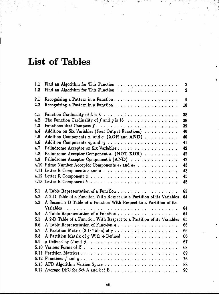
List of Tables

1.1 Find an Algorithm for This Function ....................... 21.2 Find anAlgorithm for This Function . ....... . . . . . .. 2

2.1 Recognizing a Pattern in a Function ................... . . 92.2 Recognizing a Patternin a Function ................... 10

4.1 Function Cardinality of h is 8 . .................... 384.2 The Function Caidinality of f and g is 16 ...... ...... .... 384.3 Functions that Compose f ...................... ... 394.4 Addition on Six Variables (Four Output Functions)....... ... 404.5 Addition Components a, and c, (XOR and AND)...... ... 404.6 Addition Components a2 and c 2 . . . . . . . . . . .. . . . . . . . . . 4 14.7 Palindrome Acceptor on Six Variables .............. . 424.8 Palindrome Acceptor Component a, (NOT XOR) .......... 424.9 Palindrome Acceptor Component b (AND) ......... . 424.10 Prime Number Acceptor Components a, and a2 . . . . . . . . . .. . 434.11 Letter R Components c and d ....... .............. .434.12 Letter R Component a ....... .................. . 454.13 Letter R Component b ......... ..................... 45

5.1 A Table Representation of a Function ....................... 635.2 A 2-D Table of a Function With Respect to a Partition of its Variables 645.3 A Second 2-D Table of a Function With Respect to a Partition of its

Variables ........ .................................. 645.4 A Table Representation of a Function ....................... 645.5 A 2-D Table of a Function With Respect to a Partition of its Variables 655.6 A Table Representation of Function g ....................... 665.7 A Partition Matrix (2-D Table) of g ....................... 665.8 A Partition Matrix of g With 0 Defined ..................... 665.9 g Defined by G and 0 ................................ 675.10 Various Forms of Z ................................. 685.11 Partition Matrices ................................... 695.12 Functions f and g ................................... 765.13 AFD Algorithm Version Space ........................... 885.14 Average DFC for Set A and Set B ........................ 90

xii

5.15 DFC of NN Like Architectures ........................... 915.16 AFD-DFC of NN Like Architectures .................. 935.17 Average Run-time for Set A and Set B ..................... 945.18 Run-times for Functions That Did Not Decompose ............. 955.19 Run-Times for Functions That Did Decompose ................. 96

6.1 Number of Functions for a Given DFC ....... ........... 1056.2 Number of Minority Elements Required for a Given Cost . ...... 1116.3 Addition ....... .................. ......... 1156.4 Subtraction ................ ... .............. 1166.5 Multiplication ................ .... ............. 1166.6 Modulus ............. ...... ................. 1176.7 Remainder ......... ..... ................... 1176.8 Square Root ........ ..... ................... 1186.9 Cube Root ...... ...... .... .................... 1186.10 Sine ............. ... ................... ... 1196.11 Logarithm ............ ....................... 1196.12 Miscellaneous Numerical Functions. ................ 1196.13 Primality Tests ........... ..... .............. 1206.14 Fibonacci Numbers ................. ............ 1206.15 DFC of Lucas Functions ................ ......... 1216.16 DFC of Binomial Coefficient Based Functions. ............. 1216.17 DFC of Greatest Common Divisor Function ............... 1226.18 DFC of the Determinant Function .......... ............ 1226.19 Sample Languages ........... ..................... 1246.20 DFC of Language Acceptors .......................... 1256.21 Miscellaneous String Manipulation Functions .............. 1256.22 Sorting Eight 1-Bit Numbers ......... ............... 1266.23 DFC of Sorting Four 2-Bit Numbers ......... ........... 1266.24 Input Bits Represent Arcs ......... ................. 1276.25 Additional Input Bits for Arcs to Self ................ ... 1286.26 DFC of the Various k-clique Functions on a Graph With 5 Nodes 1286.27 DFC of the Various k-clique Functions on a Graph With Four Nodes 1296.28 Turbo Pascal V5.5 Font Sets ............................ 1296.29 Character Images DFC Statistics ......................... 1306..1 3)FC and Data Compression Results for Typical Files ........... 1346.31 Data Compression Summary for Typical Files ................ 1346.32 Data Compression Summary for Atypical Files ................ 1356.33 Decomposition Summary for Non-Randomly Generated Functions . . 1376.34 Larger n Shows Greater Decomposability .................... 1386.35 Character Images ................................... 1406.36 Permutations of Variables ... ........................ 1416.37 Number of Functions and Inverses with a Given Cost Combination.. 1446.38 FERD (F) and NN (N) Error Comparison .................. 156

xiii

A. 1 Fraction of Functions Computable, by ~N.. .. .. .. .. ... ..... 189

xiv

Chapter 1

Introduction

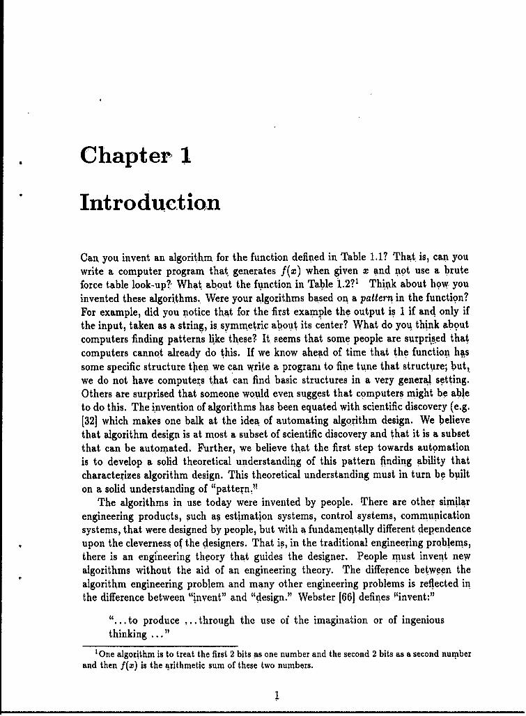
Can, you invent an algorithm for the function defined in Table 1.1? That, is, can youwrite a computer program that generates f(x) when given x and not use a bruteforce table look-up?, What about the function in Table 1.2?1 Think about how, youinvented these algorithms, Were your algorithms based on a pattern in the function?For example, did you notice that for the first example the output is 1 if and only ifthe input, taken as a string, is symmetric about its center? What do you think aboutcomputers finding patterns like these? It seems that some people are surprised thatcomputers cannot already do this. If we know ahead of time that the function h~ssome specific structure then we can write a program to fine tune that structure; buttwe do not have computers that can find basic structures in a very general setting.Others are surprised that someone would even suggest that computers might be ableto do this. The invention of algorithms has been equated with scientific discovery (e.g.[32] which makes one balk at the idea of automating algorithm design. We believethat algorithm design is at most a subset of scientific discovery and that it is a subsetthat can be automated. Further, we believe that the first step towards automationis to develop a solid theoretical understanding of this pattern finding ability thatcharacterizes algorithm design. This theoretical understanding must in turn be builton a solid understanding of "pattern.,

The algorithms in use today were invented by people. There are other similarengineering products, such as estimation systems, control systems, communicationsystems, that were designed by people, but with a fundamentally different dependenceupon the cleverness of the designers. That is, in the traditional engineering problems,there is an engineering theory that guides the designer. People must invent newalgorithms without the aid of an engineering theory. The difference between thealgorithm engineering problem and many other engineering problems is reflected inthe difference between "invent" and "design." Webster [66] defines "invent:"

"... to produce ... through the use of the imagination or of ingeniousthinking ... "

'One algorithm is to treat the first 2 bits as one number and the second 2 bits as a second numberand then f(z) is the arithmetic sum of these two numbers.

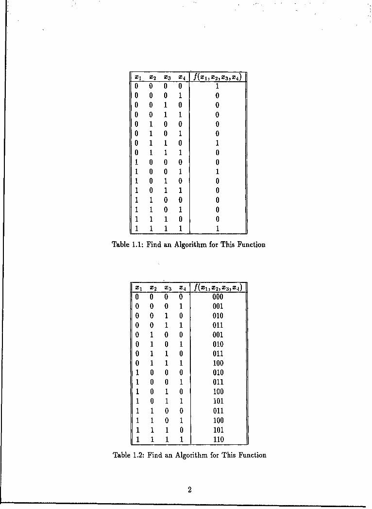
XI X2 X3 X4, f(XX2,X3,z4

0 0 0 0 10 0 0 1 00 0 1 0 00 0 1 1 00 1 0 0 00 1 0 1 00 1 1 0 10 1 1 1 01 0 0 0 01 0 0 1 11 0 1 0 01 0 1 1 01 1 0 0 01 1 0 1 0

1110 01 11 1I

Table 1.1: Find an Algorithm for This Function

XI X2 X3 X f(XI,2,XX)

0 0 0 0 0000 0 0 1 0010 0 1 0 0100 0 1 1 0110 1 0 0 0010 1 0 1 0100 1 1 0 0110 1 1 1 1001 0 0 0 0101 0 0 1 Ol1 0 1 0 1001 0 1 1 1011 1 0 0 0111 1 0 1 1001 1 1 0 1011 1 1 1 110

Table 1.2: Find an Algorithm for This Function

2

and "design:"

"... to create, fashion, execute, or construct according to plan ... "

It seems that algorithms are invented while estimation systems, control systems,etc. are designed. We believe that the difference between invention and design issimply the existence of an engineering theory. We need an engineering theory toallow algorithm design.

This report introduces "Pattern Theory." Pattern Theory consists of a formaldefinition of pattern (or structure), an approach to finding the pattern when it exists,and a characterization of various phenomena with respect to this structure. Theprincipal objective of this report is to demonstrate that many kinds of practicallyimportant patterns are well reflected in this formal definition.

Chapter 2 describes the need for an engineering theory of algorithm design. Chap.ter 3 describes Pattern Theory which is our approach to a design theory for algorithms.The key to our approach is a measure of algorithm good-ness that we call DecomposedFunction Cardinality (DFC). Chapter 4 defines this measure and relates it to the moreconventional measures. Function Decomposition is the method for optimizing withrespect to DFC. Chapter 5 develops the theory behind function decomposition anddescribes computer programs for accomplishing decompositions. We equate the ex-istence of a good algorithm for a given function and the existence of a "pattern" inthat function. So the design of a good algorithm is the same as finding the patternin a function and we think of DFC as a measure of the pattern-ness of a function.Chapter 6 reports on the results of applying this measure to a variety of fihnctions;we call this class of results "Pattern Phenomenology."

3

Chapter 2

Background

2.1 Pattern Theory

2.1.1 Introduction to Pattern Theory

The development of Pattern Theory began around 1986 at the Air Force Instituteof Technology (AFIT), Wright Patterson Air Force Base, Ohio. One of this report'sauthors, then on Long-Term Full-Time training, Prof Alan V. Lair, of AFIT's Math-ematics Department and Prof Matthew Kabrisky, of AFIT's Electrical EngineeringDepartment, all played major roles in this early work. A discussion of many of theideas that went into Pattern Theory was published in [48, 50, 511. The name "PatternTheory" was adopted after the International Conference on Pattern Recognition in1988. Our paper at that conference was in a session entitled "Fuzzy Sets and PatternTheory," All the other papers were clearly about Fuzzy Sets, so we must have beenthe Pattern Theory. A team of AART and visiting engineers continued the PatternTheory work in the in-house Pattern Based Machine Learning (PBML) project whoseresults are the subject of this report. The PBML Project is generally referred to asPattern, Theory 1 (PT 1) in this report.

2.1.2 What is a Pattern?

An Introduction to the Pattern Theory Paradigm

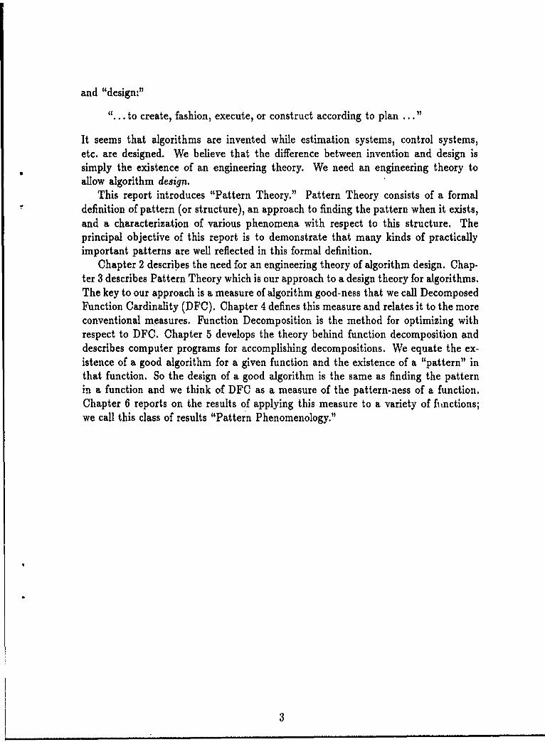
It will be useful to briefly introduce the Pattern Theory (PC) paradigm to motivatethe background. Chapter 3 is a detailed introduction to the PT paradigm. The basicproblem is how do you go from a definition of a function to a computer realizationof that function. The problem has some definition of a function as its starting pointand a computer algorithm as its solution.

We divide the kinds of information that might constitute the definition into twoclasses: samples of the function and "other" information about the function. Fig-ure 2.1 represents the algorithm design problem. The grand scheme of Pattern Theoryis to eventually complicate this flow chart slightly by allowing "learned" algorithms

5

Samples ofoteInrmin

An Algorithmfor f

Figure 2.1: The Algorithm Design Process

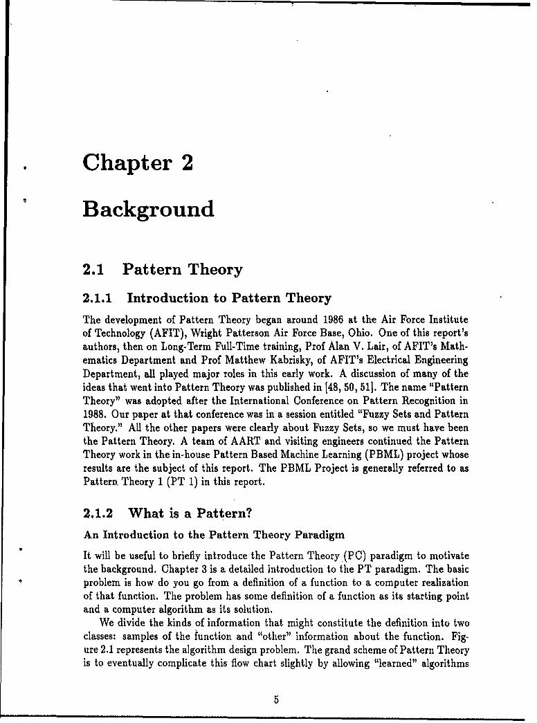
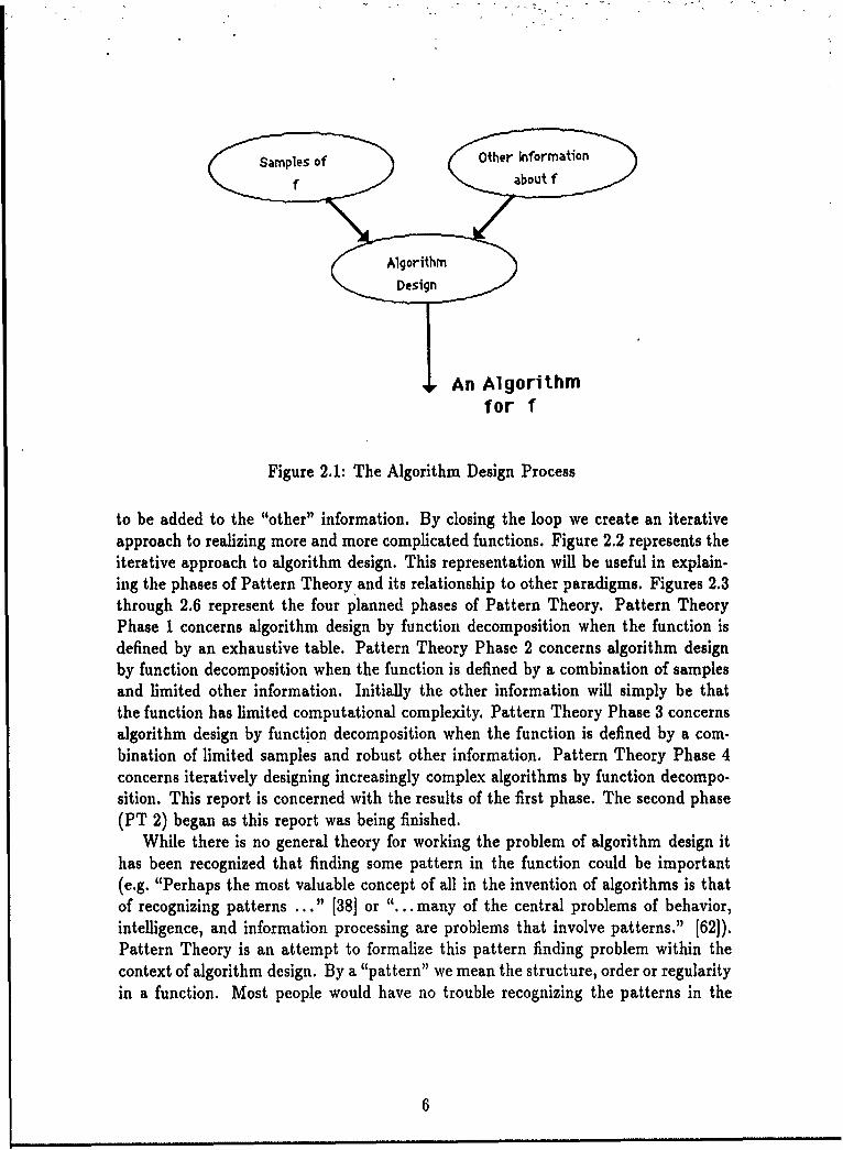
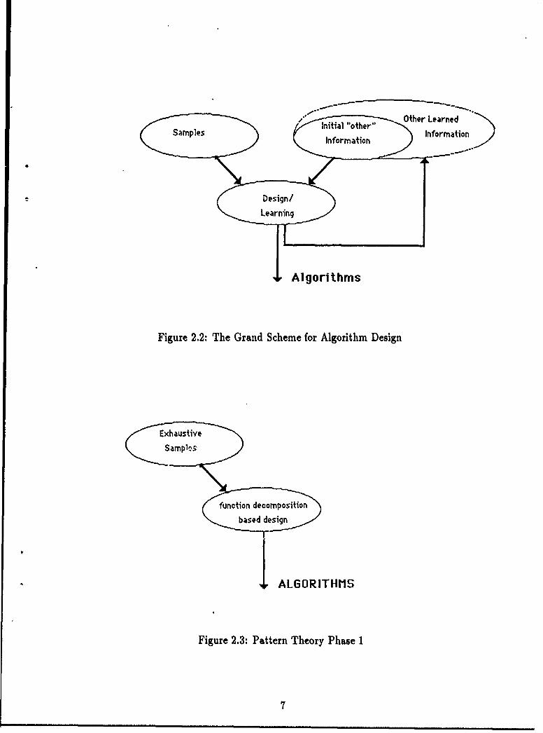
to be added to the "other" information. By closing the loop we create an iterativeapproach to realizing more and more complicated functions. Figure 2.2 represents theiterative approach to algorithm design. This representation will be useful in explain-ing the phases of Pattern Theory and its relationship to other paradigms. Figures 2.3through 2.6 represent the four planned phases of Pattern Theory. Pattern TheoryPhase I concerns algorithm design by function decomposition when the function isdefined by an exhaustive table. Pattern Theory Phase 2 concerns algorithm designby function decomposition when the function is defined by a combination of samplesand limited other information. Initially the other information will simply be thatthe function has limited computational complexity. Pattern Theory Phase 3 concernsalgorithm design by function decomposition when the function is defined by a com-bination of limited samples and robust other information. Pattern Theory Phase 4concerns iteratively designing increasingly complex algorithms by function decompo-sition. This report is concerned with the results of the first phase. The second phase(PT 2) began as this report was being finished.

While there is no general theory for working the problem of algorithm design ithas been recognized that finding some pattern in the function could be important(e.g. "Perhaps the most valuable concept of all in the invention of algorithms is thatof recognizing patterns ..." [38] or ".... many of the central problems of behavior,intelligence, and information processing are problems that involve patterns." [62]).Pattern Theory is an attempt to formalize this pattern finding problem within thecontext of algorithm design. By a "pattern" we mean the structure, order or regularityin a function. Most people would have no trouble recognizing the patterns in the

6

Initil "oher" Other Learned

SmlsInformation Information

Algorithms

Figure 2.2: The Grand Scheme for Algorithm Design

ALGORITHMS

Figure 2.3: Pattern Theory Phase 1

'7

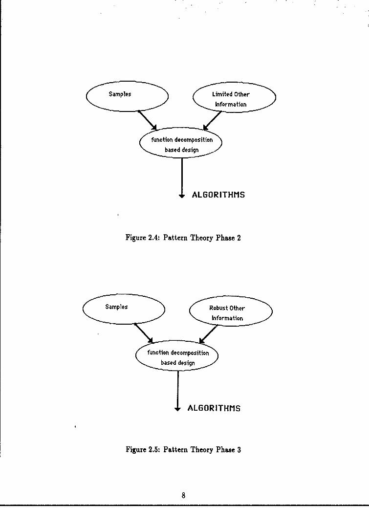
Figure .4:PaternITh oraeo2

ALGOR ITHMS


Sampes RbustOth8

• f" "Leared" "SmlsInitial Information

Information.

fn decomposition

based Design/Learning

Algorithms


X, f Wx11 12 43 94 165 256 36

Table 2.1: Recognizing a Pattern in a Function

functions defined by Table 2.11 and Table 2.22. Pattern Theory ccncerns the problem

of recognizing the patterns in functions that will allow their economical computation.But, what is a pattern?

Intuitive Ideas about Patterns

We are concerned with patterns in the sense of regularity, order, structure or theopposite of chaos. People seem to have a common sense notion of pattern-ness.This common sense notion of a pattern is supported by people's willingness to assigna pattern-ness ranking in experiments like Garner's [24] and those of Section 6.4.

Patterns can occur in many different forms. Figure 2.7 has examples of patterned

I f(X) =-22Primality test.

9

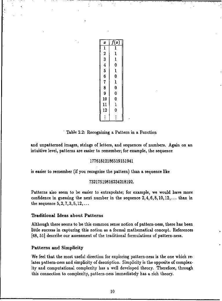
X f(x)1 1

2 13 14 05 16 07 18 09 0

10 011 112 0

Table 2.2: Recognizing a Pattern in a Function

and unpatterned images, strings of letters, and sequences of numbers. Again on anintuitive level, patterns are easier to remember; for example, the sequence

17761812186519151941

is easier to remember (if you recognize the pattern) than a sequence like

73217519816234218192.

Patterns also seem to be easier to extrapolate; for example, we would have moreconfidence in guessing the next number in the sequence 2,4,6,8,10,12,... than inthe sequence 5,2, 7,3,5,12,...

Traditional Ideas about Patterns

Although there seems to be this common sense notion of pattern-ness, there has beenlittle success in capturing this notion as a formal mathematical concept. References[48, 51] describe our assessment of the traditional formulations of pattern-ness.

Patterns and Simplicity

We feel that the most useful direction for exploring pattern-ness is the one which re-lates pattern-ness and simplicity of description. Simplicity is the opposite of complex-ity and computational complexity has a well developed theory. Therefore, throughthis connection to complexity, pattern-ness immediately has a rich theory.

10

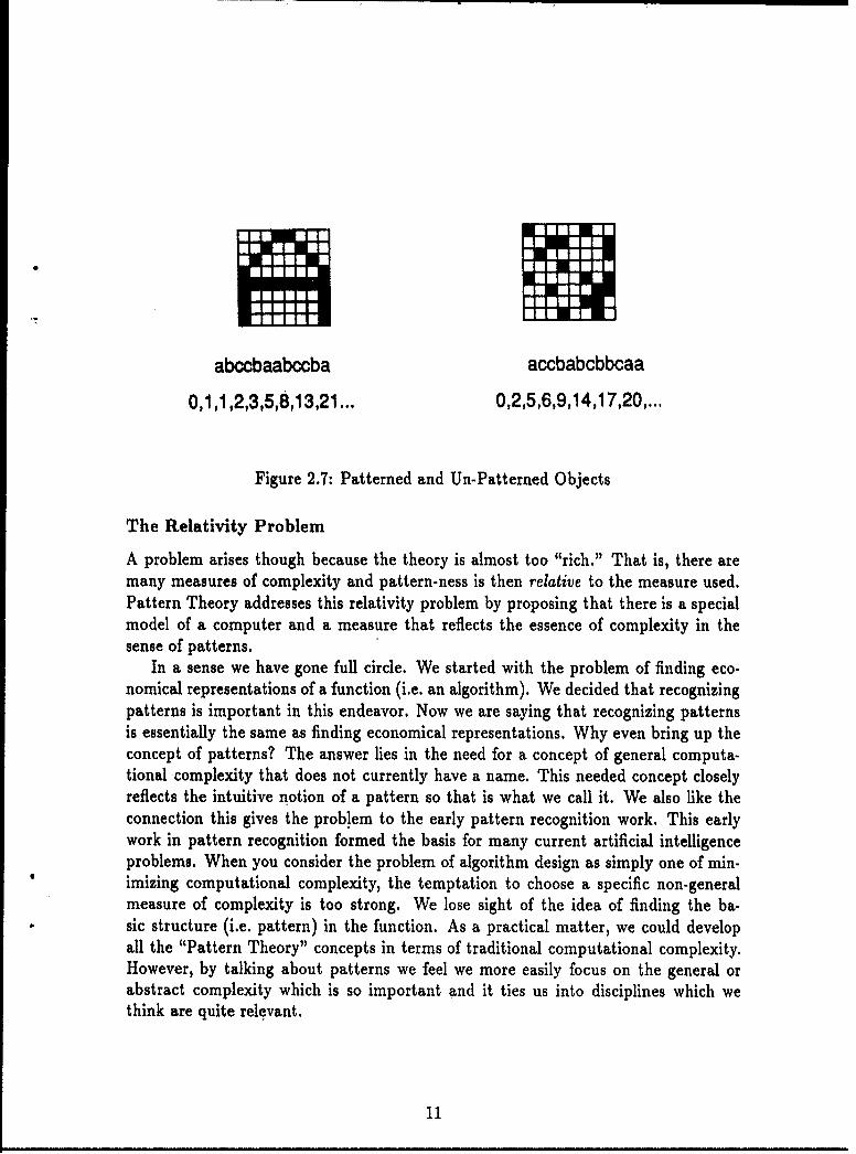
abccbaabccba accbabcbbcaa

0,1,1,2,3,5,8,13,21 ... 0,2,5,6,9,14,17,20,...

Figure 2.7: Patterned and Un-Patterned Objects

The Relativity Problem

A problem arises though because the theory is almost too "rich." That is, there aremany measures of complexity and pattern-ness is then relative to the measure used.Pattern Theory addresses this relativity problem by proposing that there is a specialmodel of a computer and a measure that reflects the essence of complexity in thesense of patterns.

In a sense we have gone full circle. We started with the problem of finding eco-nomical representations of a function (i.e. an algorithm). We decided that recognizingpatterns is important in this endeavor. Now we are saying that recognizing patternsis essentially the same as finding economical representations. Why even bring up theconcept of patterns? The answer lies in the need for a concept of general computa-tional complexity that does not currently have a name. This needed concept closelyreflects the intuitive notion of a pattern so that is what we call it. We also like theconnection this gives the problem to the early pattern recognition work. This earlywork in pattern recognition formed the basis for many current artificial intelligenceproblems. When you consider the problem of algorithm design as simply one of min-imizing computational complexity, the temptation to choose a specific non-generalmeasure of complexity is too strong. We lose sight of the idea of finding the ba-sic structure (i.e. pattern) in the function. As a practical matter, we could developall the "Pattern Theory" concepts in terms of traditional computational complexity.However, by talking about patterns we feel we more easily focus on the general orabstract complexity which is so important and it ties us into disciplines which wethink are quite relevant.

11

2.2 Background of Related Disciplines

2.2.1 Recognizing Patterns - the Many Disciplines

In the following we will survey the disciplines relevant to Pattern Theory. Perhaps themost obvious discipline is pattern recognition (e.g. [16, 22, 29]). However, the modernappc,)aches to pattern recognition do not treat patterns in our special sense. Thisposition is developed in [48, 51]. Early pattern recognition research was concernedwith special patterns, as are elements of modern research (e.g. [58, 63]). At onetime, Pattern Recognition (PR) and Artificial Intelligence (AI) research had a greatdeal in common. This common philosophical base is quite relevant to Pattern Theory.However, the specific disciplines within PR and AI (e.g. statistical pattern recognition,syntactic pattern recognition, expert systems, neural nets) seem to have all divergedfrom the core problem. In all these disciplines, the basic structure of the problem mustbe recognized by the designer without theoretical tools or automation. Only after thisbasic structure is defined can theoretical tools or anything approaching automationbe applied. Data Compression (e.g. [27]) can be considered as a problem of findingand exploiting patterns in data. This has an obvious connection with our problem.Within the data compression discipline the patterns are recognized by the designer ofthe data compression routine, again without theoretical tools or automation. As wehave already mentioned, the complexity and computability disciplines of theoreticalcomputer science are most related to Pattern Theory. We will make extensive useof computational complexity results. We will also show that computability is a sub-problem of complexity and of no special interest within our context (see Appendix A).Finally, the problem of designing electronic circuits (switching theory) is connectedto Pattern Theory. We will see that with respect to our generalized measure ofcomplexity, designing efficient circuits and designing efficient algorithms are the sameproblem. As you would expect, both problems depend on finding some pattern inthe function to be realized. We make extensive use of function decomposition theorywith was originally developed within the switching theory context.

2.2.2 Pattern Recognition

The relationship between the traditional field of pattern recognition and PatternTheory is discussed in depth in [48, 49]. The following is a brief summary of thatdiscussion.

The subject of pattern recognition can be divided up many ways. The mostcommon is to consider the fields of statistical (also decision-theoretic, geometric orvector space) pattern recognition, syntactic (also structural or linguistic) patternrecognition and fuzzy methods of pattern recognition. The references [48, 49] usea slightly different division, emphasizing the role of apriori structure in designingrecognizers. The a priori structure is the representation system or language used toexpress the recognition algorithm. Pattern Theory is an attempt to generalize thisidea of a priori structure. Therefore, the role of a priori structure within traditional

12

pattern recognition is especially relevant. Most traditional pattern recognition isbased on either a geometric or a syntactic structure. Reference [48] discusses thebackground of traditional pattern recognition in terms of these two structures.

The basic disconnect between Pattern Recognition and Pattern Theory lies in ourbelief that the interesting pattern finding phenomenon occurs in the design of recog-nition systems rather than in their operation. Reference [51] explains this position.This difference in perspective is reflected in the different approaches to research. InPattern Recognition it is generally believed that a researcher should choose a singlerealistic problem (typically speech or character recognition). The PT approach is tostudy many simple problems (e.g. Chapter 6 reports on over 1000 different functions).The concern is that when we study only a single function, the researcher ends up do-ing the pattern finding and the so-called "pattern recognition" algorithm is simplya realization of the patterns recognized by the researcher. Studying many differentkinds of functions makes it more difficult for the researcher to insert (deliberately orunconsciously) any humanly recognized patterns. This forces the machine to do sometrue pattern finding.

2.2.3 Artificial Intelligence

Machine learning, a problem of artificial intelligence (AI), might be thought of asan attempt to automate the process that we seek to understand. That is, we wantto understand the process of defining an algorithm while machine learning seeksto automatically generate an algorithm. Therefore, Pattern Theory has a strongconnection to machine learning.

We think of the artificial intelligence approach to this problem as one of figuringout how people do it and then attempting to model that process on a computer. Forexample, expert systems derive from the cognitive psychology model of thought andneural nets derive from the physiological model of the hardware involved in thought.It is possible that Al will come up with useful systems based on this approach withoutany understanding of the process at an abstract level. An often used e'nalogy for AIis the problem of manned flight. In this analogy the AI approach would be analogousto the artificial bird approach. That is, we could design machines with bird-likeproperties since a bird is an existing system which performs the desired function. Weare trying to take what might be called the "Wright" approach. That is we seek tounderstand the basic phenomenon that will allow us to design from first principles.This approach will not immediately lead to systems with practical value; however, webelieve it is the only approach to continuing long term improvements.

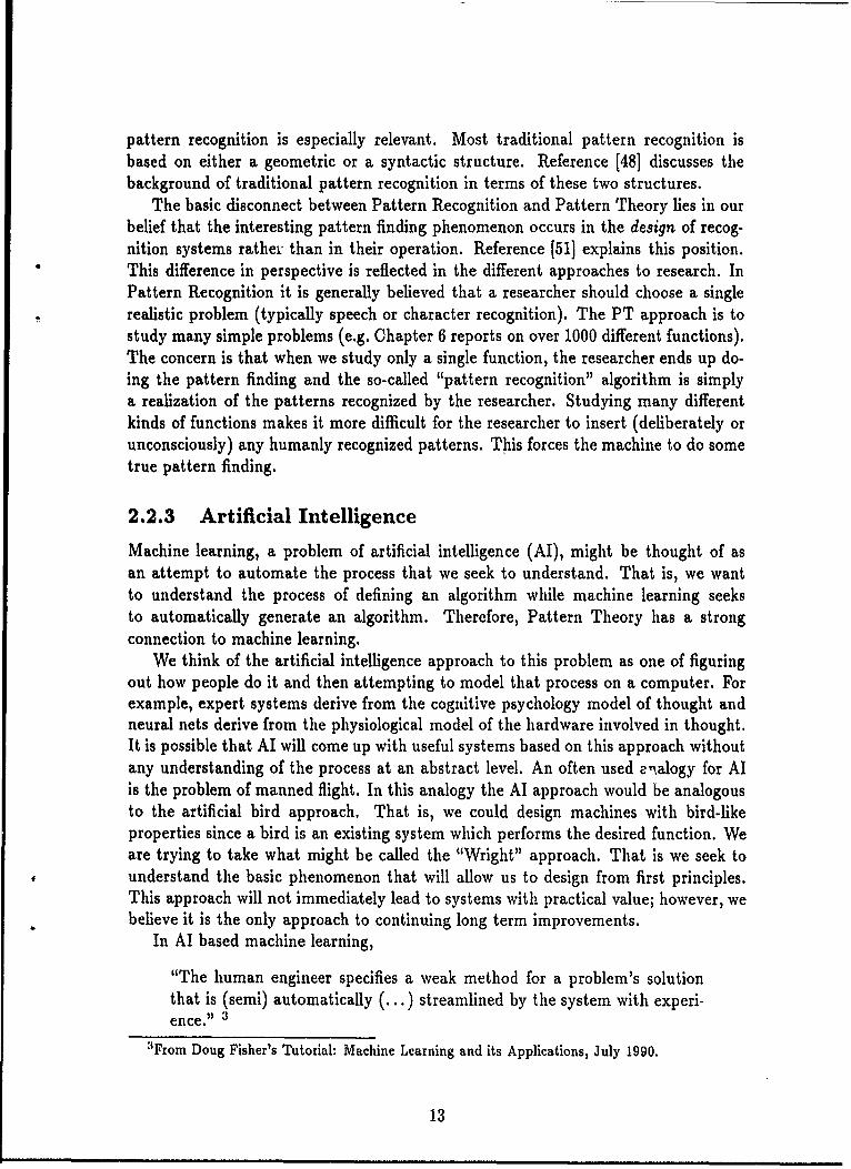
In AI based machine learning,

"The human engineer specifies a weak method for a problem's solutionthat is (semi) automatically (...) streamlined by the system with experi-ence." 13

"From Doug Fisher's Tutorial: Machine Learning and its Applications, July 1990.

13

-NN

Figure 2.8: Neural Net Paradigm

We feel that the so called "weak method" constitutes a large fraction of the overallsolution. The problem addressed in Pattern Theory includes the development of aweak method as well as the "automatic streamlining."

There are many approaches to machine learning. Learning within the context ofexpert systems include rule learning (e.g. [13]), adaptive figure-of-merits to improvenon-exhaustive searches (e.g. [13]), and genetic algorithms (e.g. [15]). Some neuralnets learn [53]. Within the discipline of pattern recognition there are learning methodsfor both geometric (e.g. [16]) and syntactic (e.g. [22]) systems. Adaptive systems (e.g.[37]) as used in estimation and control theory for non-linear systems have as manylearning characteristics as Al systems.

We can characterize machine learning systems using the diagram in Figure 2.1.The "other" information includes an assumption that the desired function has arealization of the form used by the learning system. Take Neural Nets for example(Figure 2.8), the "other information" is an assumption that the desired functionmay be represented by the chosen architecture of thresholded linear combinations.Appendix A demonstrates that this assumption is surprisingly restrictive. The designapproach then is back-propagation or some other method of assigning weights. Thetraditional machine learning paradigms are built around a specific structure. The keyidea of Pattern Theory is that we want to find the structure that already exists inthe function. We do not want to try to force fit a function to some structure that wechose ahead of time.

One Al approach, known as Abduction [44], uses the "chunking" idea of Miller [43].The function decomposition approach of Pattern Theory also exhibits this chunkingidea.

14

2.2.4 Algorithm Design

The texts on algorithm design (e.g. [3]) are quite different from the texts on mostother electrical engineering design problems (e.g. circuit design, control system de-sign, communications system design). Most electrical engineering design texts tell, inan almost cookbook fashion, how to solve problems of a given type. Typically youbegin by developing a dynamic model of the system involved. Next, you apply somevery general principles, such as modulation in communications or feedback in con-trols. Then there are some mathematically rigorous tools for optimizing the design.Finally there are methods for predicting performance and evaluating the design. Bycontrast, texts on algorithm design give a list of specific algorithms that you are tomix and match to your problem. They do not tell you how to come up with a newalgorithm. If controls texts were like algorithm design texts they might give a table offeedback gains for specific plants and specific desired step responses, but they wouldnot give the general relationship between feedback gain and system performance thatcontrol theory actually provides. It seems that if an engineer with a good under-standing of control theory were to compete in solving a new controls problem with anengineer with no controls background, the engineer with knowledge of control theorywould arrive at a much better design. However, if two engineers were to competeat discovering a new algorithm, the engineer with a background in algorithm designwould seem to have little advantage (unless, of course, some previously discovered al-gorithm happened to fit the new problem). In summary, although you can find textson algorithm design, they do not address design of fundamentally new algorithms.

In the introduction of an algorithm design text they may mention a general prin-ciple of algorithm design know as "divide and conquer," e.g. [7, p.3]. The functiondecomposition approach of Pattern Theory can be thought of as a formalization ofthe divide and conquer principle.

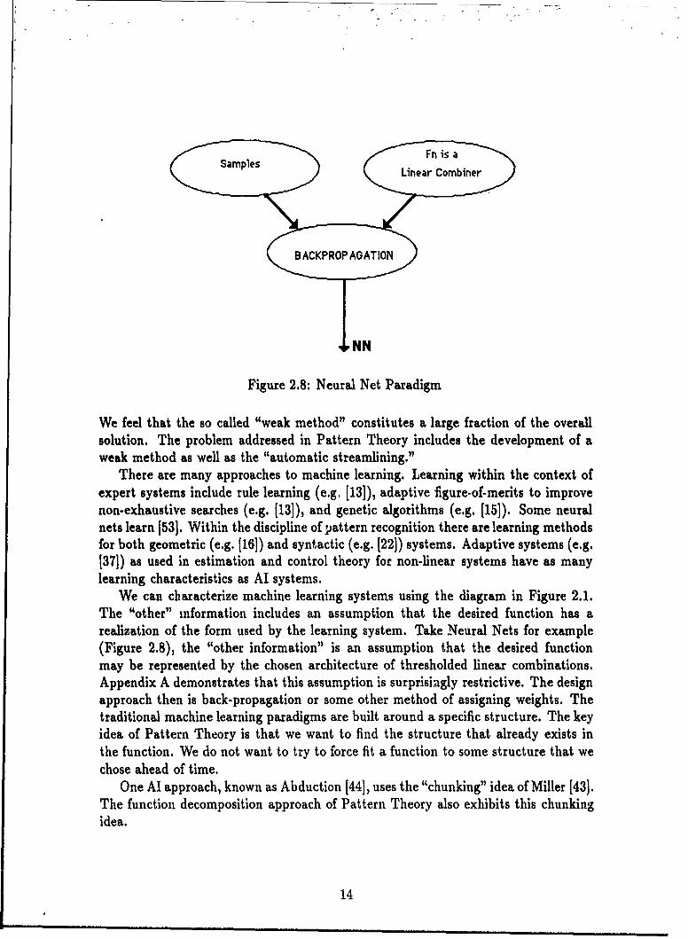
An important technology that is being developed and used in the Avionics Di-rectorate is Model-Based Reasoning, especially its application to target recognition.From a Pattern Theory perspective, Model-Based Reasoning is not too different fromtraditional algorithm design. Referring again to Figure 2.1, model-based simplymeans that the "other" information is a collection of models. The algorithm de-sign problem is classical; that is, we are left to our own inventiveness to turn themodels into an algorithm (Figure 2.9).

2.2.5 Computability

The problem of computability would seem to be quite relevant to Pattern Theory.But it is not. Computability, in its formal sense, is tied to recursion.

"... because all evidence indicates that the class of partial recursive func-tions is exactly the class of effectively computable functions; ... " 1351

It seems clear that recursion is a desirable property in a function, but it is neither nec-essary nor sufficient for a function to be patterned. We say this because all functions

15

Algorithm

Figure 2.9: Model-Based Reasoning Paradigm

of interest in practical computing are finite; all finite functions are partial recursive;yet finite functions are not practically computable with high probability. There are ofcourse many infinite functions (especially those on the real or natural numbers) thatare of interest, but we never really try to compute them. We would always be satis-fied with the ability to compute these function on some finite sub-domain. Therefore,the use of (and complete dependence on) infinite functions for interesting results incomputability makes it of no practical use in Pattern Theory. We will argue laterthat recursion is of secondary importance in the general complexity used in PatternTheory. Appendix A develops some classical computability results from a PatternTheory perspective.

2.2.6 Computational Complexity

As we have mentioned, "Pattern Theory" might more appropriately be an un-namedsub-set of computational complexity theory. The theory of computational complexity(e.g. [33, 54, 64]) has well developed measures of complexity. The measures used inPattern Theory are a special case of these. There are also many computiing theory re-sults in what we call Pattern Phenomenology. However, complexity theory is orientedtowards analysis rather than the synthesis of computational systems. Sections 4.4 and4.5 develop the relationship between conventional measures of complexity and PatternTheory.

2.2.7 Data Compression

The design of a data compression system depends upon recognizing and exploitingsome pattern in the data. However, like algorithm design texts, data compression

16

texts (e.g. [271) give you a list of specific procedures for some common patterns thatwere recognized by people. They do not tell you how to find new patterns in data.

2.2.8 Cryptography

Cryptography is concerned with patterns in sequences rather than functions. Al-though any mathematician will tell you that a sequence is a function, the problemis somewhat different. Pattern theory has so far been concerned with patterns infunctions. Although the problem of breaking codes must involve pattern finding inthe sense of Pattern Theory, we have not explored how Pattern Theory relates tocryptography.

2.2,9 Switching Theory

From a Pattern Theory perspective, the design of electronic circuits is essentially thesame as algorithm design. Unlike algorithm design though, there are many theoreticalsynthesis tools. There seem to be three approaches to the design of discrete circuits.One approach (e.g. [21]), using ROM or PLA's, uses an essentially brute force tablelook-up. This approach offers no special insight into the pattern finding problem. Asecond approach is to design optimal two-level circuits [21]. This approach does notcapture patterns in a sufficiently general sense because some highly patterned func-tions (e.g. the parity function) do not have efficient two-level realizations. The thirdapproach is based on function decomposition. The idea of function decompositionhas been around a long time (see [41), but it has had a limited role in circuit design.Function decomposition is not even mentioned in many standard Switching Theorytexts (e.g. [21, 26, 45]). When function decomposition is discussed (e.g. [60]), thereseems to be general agreement that function decomposition is "prohibitively labo-rious." We believe that function decomposition gets at the crux of computationalcomplexity. The practical difficulties of using function decomposition for circuit de-sign does not detract from its central theoretical role. If nothing else, we hope thatPattern Theory will contribute to the realization that function decomposition is a (ifnot the) fundamental problem in computer science.

2.2.10 Summary

There are many disciplines that are relevant to Pattern Theory. As Pattern Theorymatures there will be many potential areas of application. There are also many resultsfrom these related fields that are useful in Pattern Theory. We especially use somecomplexity ideas from computing theory and the function decomposition idea fromswitching theory.

17

Chapter 3

The Pattern Theory Paradigm

3.1 Why is Pattern Theory Needed?

This section will attempt to motivate the Pattern Theory work. This motivation isdeveloped by picking a particular problem, discussing the importance of computingin solving this problem, discussing the role of algorithms in doing computing, and,finally, discussing the need for a theory to design algorithms.

3.1.1 Offensive Avionics as a Potential Application

The Pattern Theory work was performed in the Mission Avionics Division of theAvionics Directorate of Wright Laboratory (WL/AART). This organization has of-fensive avionics algorithms as a principal product. Therefore; we use this potentialapplication of an algorithm design theory as an example to motivate the need for sucha theory. The arguments used here could have been couched in terms of any one ofthe many diverse problems requiring algorithms (see Section 2.2). We chose offensiveavionics algorithms because we are most familiar with this application and it helpsexplain why it is appropriate for Pattern Theory work to be done in this organization.

3.1.2 Importance of Computing Power in Offensive Avion-ics

Offensive avionics (or fire control) is responsible for locating, identifying and selectingtargets, appropriately releasing weapons and doing this in the most survivable mannerpossible. In order to better understand what must be done to meet the responsibilitiesof fire control, we often think of fire control as a family of functions. These functionsserve one of two purposes. Either they are part of the overall sensor system or they arepart of the control system. The sensor system attempts to determine the "state-of-the-world," which includes targets, self, threats, cooperating friendlies and anythingelse that could be a factor. The control system manages all the resources of theaircraft. This includes deciding on the specific trajectory for the aircraft, managing

19

the sensors, as well as managing the weapons themselves.All these functions have always been part of the fire control problem. At one

time, the "weapon system" was just a person. This person formed their state-of-the-world picture from what they could see and hear. They moved into position on footand instinctively planned and executed their "weapon delivery" (perhaps a punch orkick). Over time, people began to use artificial weapons, at first sticks and stones buteventually guns and bombs. We began to use artificial sensors such as telescopes andradars. We also developed artificial means of locomotion, beginning with horses andeventually leading to airplanes. We have added these increasingly sophisticated ma-chines to a person always trying to improve the overall weapon system performance.Until recently, the extremely adaptive nature of people has allowed them to do theirstate-of-the-world assessment, their planning and control functions and to use thesemachines effectively. However, there has been an explosion in the complexity of theweapon systems. Now we not only have an artificial sensor, we have multiple sensors,each capable of measuring multiple attributes of many targets. Our artificial weaponsnow include many types, some with long range and many degrees of flexibility. Ourmeans of getting about have become faster and more maneuverable.

At first we tried to deal with the increasing complexity by putting more peoplein the system. The crew size for bombers was six when we built the B-52. Then,as computers and software technology became available we began to deal with thecomplexity more and more through aids and automation. The crew of the B-1 wasdown to four and the B-2 has only two crew members.

What technology has allowed the crew size to decrease despite an increase inthe complexity of the task? What technology may eventually allow the crew sizeto go to zero? The crew provides no useful work in the force times distance sense.Their sensory capabilities, in terms of being able to resolve and detect light, sound oracceleration could be easily replaced. People are in modern combat aircraft for onereason: their computing power. Therefore, it is fair to say that computing power isan extremely important technology for avionics systems.

3.1.3 Importance of Algorithms in Computing Power

In the preceding section we discussed the importance of computing power. Now wewant to discuss how important algorithms are in overall computing power. We canthink of computing power as being made up of three technologies. One technologyis computing hardware. Fairly good measures of hardware capability exist in termsof Instructions per Second, Operations per Second, etc. There has been tremendousgrowth in computing hardware technology. In addition to hardware, effective compu-tation requires software. We like to think of this software as being developed in twostages. First there must be some algorithm that describes the desired computation atan abstract level. Then this algorithm must be implemented in a specific computerlanguage. We consider the first problem to be algorithm design and the second prob-lem to be software engineering. These problems are not entirely separable, just as thehardware and software problems are not entirely separable; however, it is useful to

20

Runtime1.000E+ 10 - [

1.000E+09 The 'normal' complexity Is exponential.

1.000E+0810000000 Algorithms are-cubic or better.

1000000100000

1o000

101'

0 ,1 1-- A -, I I , I I I . . . , i .

0 2 4 6 8 10 12 14 16 18 20 22 24 26 28 30

Number of Input Bits- Exponential --- Cubic

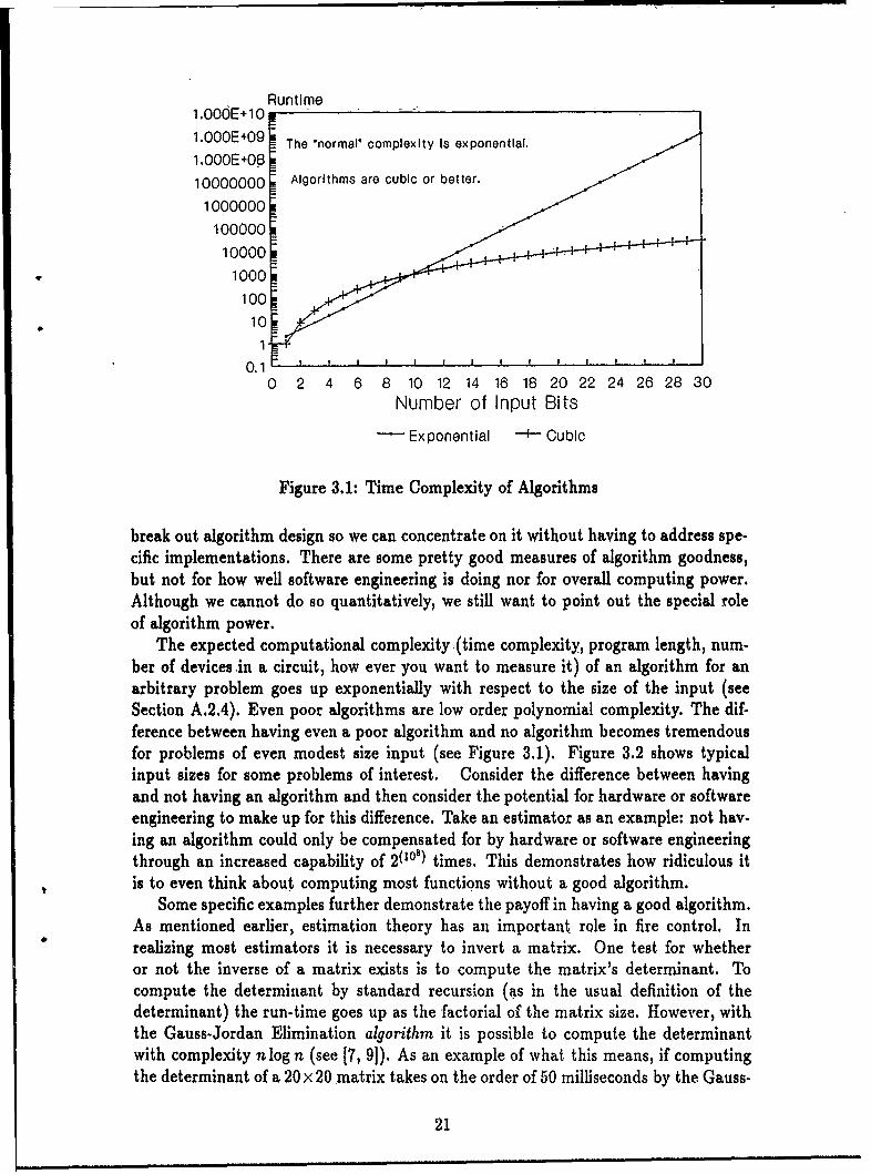
Figure 3.1: Time Complexity of Algorithms

break out algorithm design so we can concentrate on it without having to address spe-cific implementations. There are some pretty good measures of algorithm goodness,but not for how well software engineering is doing nor for overall computing power.Although we cannot do so quantitatively, we still want to point out the special roleof algorithm power.

The expected computational complexity -(time complexity, program length, num-ber of devices in a circuit, how ever you want to measure it) of an algorithm for anarbitrary problem goes up exponentially with respect to the size of the input (seeSection A.2.4). Even poor algorithms are low order polynomial complexity. The dif-ference between having even a poor algorithm and no algorithm becomes tremendousfor problems of even modest size input (see Figure 3.1). Figure 3.2 shows typicalinput sizes for some problems of interest. Consider the difference between havingand not having an algorithm and then consider the potential for hardware or softwareengineering to make up for this difference. Take an estimator as an example: not hav-ing an algorithm could only be compensated for by hardware or software engineeringthrough an increased capability of 2(ls) times. This demonstrates how ridiculous itis to even think about computing most functions without a good algorithm.

Some specific examples further demonstrate the payoff in having a good algorithm.As mentioned earlier, estimation theory has an important role in fire control. Inrealizing most estimators it is necessary to invert a matrix. One test for whetheror not the inverse of a matrix exists is to compute the matrix's determinant. Tocompute the determinant by standard recursion (as in the usual definition of thedeterminant) the run-time goes up as the factorial of the matrix size. However, withthe Gauss-Jordan Elimination algorithm it is possible to compute the determinantwith complexity n log n (see [7, 9]). As an example of what this means, if computingthe determinant of a 20 x 20 matrix takes on the order of 50 milliseconds by the Gauss-

21

Agoic .. Number of Binary Variables

Algorithm Design :to evaluate 16 ................................................... 1012

Estimator 1Oe.lO12

ATR 1osIFFN Fusion 104Clhnruclor flucognillon 1o'Missile Envelope 1oControl Law 2SO.103

Library Functions 16 ....................... 64

Data Compression : to store 13 ...................... 46Video 32 .... 46Audio 19 ..... 32

Large S1W or Data Bases 19....29Pictures 13 ...... 27Airborne/PC S/W or Data 13-21

Digital Circuit Design 4 ...... 16I )n

0 10 20 30 40 50 100 10, 105 106 1012

Figure 3.2: Typical Algorithm Input Sizes

Jordan Elimination method then it would take on the order of 10 million years by thestandard recursion method. Sorting a list with Insertion sort has complexity n2 (570minutes to sort 100,000 elements) while Quick sort has complexity n log n (30 secondsto sort 100,000 elements). The relatively recent invention of algorithms like QuickSort has brought about many of the word processing features that we use everyday.Even minor improvements in an algorithm can have dramatic effects. For example, theinvention of the Fast Fourier Transform (FFT) algorithm only reduced the complexityfrom n2 to nlog n (see [46]). However, without the FFT algorithm, today's real timedigital Synthetic Aperture Radar (SAR) capability could only be achieved with ahardware throughput improvement of about five orders of magnitude. Note that theFFT and Quick Sort algorithms were "invented." Without an engineering theory,things are invented. With an engineering theory, things are designed.

Therefore, good algorithms are very important in effective computing and in areal sense more important than hardware or software engineering.

3.1.4 Role of a "Design Theory"

We have gone from recognizing the need for computing power to the need for algo-rithms; now we want to recognize the need for an engineering theory to help designalgorithms. But before we do that, we review the role of an engineering theory indesign.

Although there are some particular well established engineering design theories(e.g. Modern Control Theory or Estimation Theory) there does not seem to be muchliterature on these kinds of theories in general. There is a body of literature onmethods to improve the creativity of designers (e.g. [6, 17]). There is also some workon a theory about design (e.g. [28]). However, these do not treat "design theory"

22

in the desired sense. The most relevant literature about engineering design concerns"optimal design" (e.g. [47, 57]). In this literature the design process is one of defininga model, establishing the criteria for a good design and then optimizing the designwith respect to that criteria. While most of the traditional optimal design theorieshave quantitative criteria and specific methods for optimization, they would be ofvalue even without that. A good design theory tells you what is important about aclass of problems, tells you about some absolute limits on performance, allows youto predict performance, and gives you some specific steps towards solving a class ofproblems. For example, estimation theory (e.g. [36]) tells you that it is important tomodel the dynamic behavior of the system (i.e. X = AX + BU-) and the measurementprocess (i.e. Z = HX- + Gzi) as well as the specific form of an optimal estimator basedon these models. Estimation theory also allows you to determine any observabilitylimitations. Ideally, a design theory would have a formal structure. As Melsa andCohn [39] say in regards to decision and estimation theory:

"Although we treat such problems intuitively all the time, it is importantthat we cast them into a more definite mathematical model in order todevelop a rigorous structure for stating them, solving them, and evaluatingtheir solution."

By a mathematical model we would not necessarily mean a numerical model, onlythat the model have a formal logical structure.

A good design theory is not the solution to any particular problem; rather, it is atool useful in solving a whole class of problems.

3.1.5 The Need for a Design Theory for Algorithms

Historically, Electrical Engineering design theories (especially estimation -and controltheory) have been used to develop fire control algoithms. However, the modern firecontrol problem requires a large variety of algorithms. Many of tihese problems areeither not naturally representable as estimation or control problems or the solutionsprovided by these traditional theories are computationally intractable. For example,the determination of an aircraft trajectory for attacking multiple ground targets in asingle pass can be set up as an optimal controls problem. However, because closedform optimal solutions cannot be found, this leads to a computationally impracticaldesign. Further, the problem of selecting a trajectory for the attack of multipleairborne targets cannot even be set up as a reasonable controls problem. The pointwe are trying to make is that there is a need for a more general theory of algorithmdesign. Our recognition of this need arose in considering fire control problems butthe need is pervasive in the application of computing power.

With the extensive literature on algorithms it seems surprising that there is nota general theory of algorithm design. However, most of this literature is concernedwith the analysis of algorithms rather than their design. Even the literature onalgorithm design typically does not discuss how to create an algorithm; rather they tellyou how to apply known algorithms in various situations. When algorithm creation

23

is discussed, it is in terms of "discover" or "invent" rather than design (e.g. "The'discovery' by Cooley and Tukey in 1965 of a fast algorithm ... " [71 or "The creationof an algorithm . .. , is an inventive process ... " [38] ).

Once connected with the problem of "discovery", we begin to wonder if a designtheory for algorithms is even possible. Reference [31] argues that it is not onlyrossible to have a theory of the discovery process but that it is possible to automatethe process. While we think they are correct, this report is concerned with simplytrying to understand algorithm design in a formal theoretical sense. We feel that athorough understanding of the problem is the first step to a useful design theory andthat design assisted by an engineering theory would logically precede automation ofalgorithm design.

3.1.6 Summary

This section attempts to show the practical relevance of Pattern Theory. We beganby discussing the importance of computing in offensive avionics; although the impor-tance of computing could have been derived from many sources. We then point outthe special dependence that computing power has on algorithm design. Improvedhardware or software engineering are fine tuning compared to new algorithms whichcreate entirely new capabilities. After clarifying what we mean by a "design theory,"we explain that a design theory for algorithms would be very beneficial and that sucha theory does not currently exist. The bottom line is that there is a strong, un-met,need for a theory of algorithm design.

3.2 The Pattern Theory ApproachPattern Theory is an attempt at an engineering design theory for algorithms. Thissection will present the algorithm design problem in a way consistent with an engi-neering theory. We begin by first expanding on our concept of a design theory.

3.2.1 The "Given and Find" Characterization of a DesignTheory

We will develop our concept of a design theory in terms of "givens" and "finds." Givenand Find are intermediate stages in going from the real problem to the real solution.The design theory provides methods for relating the given problem statement to whatwe want to find. However, there always remains the task of couching the real designproblem into a simplified problem of specific givens and finds such that the designtheory can be applied.

Many engineers first encounter a design theory in Statics. Therefore, we use aproblem from statics as our example, from [40]. The real problem is to design a roofthat will support whatever snow, wind, etc. that will stress it. The first step in goingfrom the "real problem" to the "given" for the design problem is to select some form

24

of truss. For example, a Howe truss could be selected. This selection might be basedon the designer's recognition that it is appropriate for this class of problem, but isoutside the design theory. A second step in going from the "real problem" to the"given" for the design problem is to make some assumptions about the loads thatwill be applied to the truss. These assumptions take the form of a certain magnitudeforce applied at certain points on the truss. These assumptions might be based onthe designer's knowledge of local weather, etc.; but again, this is outside the designtheory. We have gone from the "real problem" to a set of "givens." This part ofthe design is not based on any "design theory," rather it depends upon the humanelement in design.

The "real solution" to this problem might consist of a complete specification ofmaterials in the truss, the size and shape of the members of the truss, how themembers are joined, etc. The designer recognizes that if the forces in the memberscan be found, then it would be easier to complete the real problem. For example,a catalog could be used to select truss members on ce the maximum load on a givenmember was known. Therefore, we say the "find" is the force in each member. Again,going from the "find" to the "real solution" will not be aided by the design theory.However, now that we have specific "givens" and "finds," we can apply the "designtheory" of Statics to connect these two. In particular, given the loads on a particulartruss we can solve for the forces in each member of the truss.

In summary, a design theory operates within the simplified environment of specific"givens" and "finds." The messy problems of determining the "givens" from the realproblem and the real solution from the "finds" are outside the theory. Pattern Theoryis an attempt at a design theory in this sense for algorithms.

3.2.2 Definition, Analysis and Specialization

It is important that a design theory begin with a well-defined problem. CharlesKettering is reported to have said:

"A problem well stated is a problem half solved."

Our approach to stating the problem is to first define a very general and abstractproblem (Section 3.3). A problem is well-defined when we can say precisely what isgiven, what is to be found and the criteria by which the solutions are to be judged.The problem will then be analyzed to determine how it might be partitioned intosimpler problems. Finally, we specialize to one of the simpler problems (Section 3.4.9).We deliberately and explicitly set aside some aspects of the problem. There are twopurposes to this approach. First, it allows us to arrive at a well-defined and potentiallysolvable problem. Second, it allows us to understand how our problem is a specialcase of more general problems.

25

3.3 The General Problem of Computational Sys-tem Design

Here we develop the most general Pattern Theory problem. This problem is a centralpart of many disciplines (c.f. Chapter 2). First we must deal with several rathergeneral, almost philosophical, issues. We will explain why we are especially interestedin recognizing patterns in functions, the meaning of a representation of a function,and figures-of-merit for competing designs.

3.3.1 Computation and Functions

We can imagine trying to recognize patterns in all kinds of mathematical objects.The examples of Section 2.1 were typically sequences. However, we believe thatfunctions have a unique importance when considering pattern finding in connectionwith computation.

First of all, functions are a fundamental mathematical concept. A function f is aset of ordered pairs from X x Y such that for all (x1,yi) and (X2,42) in f, if x, = Z2

then y, = Y2. This definition of a function only requires some set theory, order, andlogic as background.

The only trick to being a function is that there be only one output for any giveninput. For example, in an Automatic Target Recognition setting our assumption isthat there i. ;:zctly one desired output (e.g. target type) for each input (e.g. animage). This assunption does not preclude the output from having probabilities; inthis case our assumption only requires that there be exactly one desired output prob-ability distribution (e.g. p(tank) = 0.1, p(truck) = 0.6, p(tree) = 0.2, ... ) for eachinput. Our assumption does preclude those cases where there are a significant numberof inputs for which multiple possible outputs would be acceptable. For example, ifwe consider outputs of either 0.99 or 1.0 to be acceptable then our assumption doesnot hold. While this may seem to be the more common situation, it is possible todefine a codomain for almost any real problem such that the assumption does hold.For example, we could define "0.99 or 1.0" as a single output value.

Functions are also abstractions of most of the traditional models of computation.Language acceptance is a common model for computation in the theory of computing.Language acceptance is a special case of a function; that is, a language acceptor is afunction from a set of strings into the binary set {accept, reject}. Problem solving isa common model of computation in computing theory and some artificial intelligencecontexts. Problem solving is a function from a set of problem definitions into the set ofpossible solutions. Decision making is also a function from the factors in the decisioninto the set of possible decisions. Functions are a "show me" approach to modelingknowledge. What a computer (or person) knows is exactly the set of questions thatit can answer. We would say that knowledge is well represented by a function froma set of questions into a set of answers. Reference [49] discusses this relationshipbetween mathematical functions and knowledge at length. Many models of machine

26

learning, e.g.[13, p.326] or [42, p.6], can also be interpreted as special cases of functionrealization.

Non-function computation problems exist, such as the generation of one-way com-munications (radio/TV) or clocks, but virtually all conventional computing is welmodeled by functions.

In summary, a function is an extremely general and well-defined model for com-putation. When we talk about computation we are talking about realizing a function.

3.3.2 Representation

The notion of representation is very important in Pattern Theory (see [49, pp.29-50]).The design problem begins with some sort of a representation of a function and thenwe want to find an efficient algorithm that will also be a representation of that samefunction. Therefore, the design problem is one of translating representations.

The representation of a function is meaningful only if there is some agreed to"representation system." The representation system is kind of like the syntax andsemantics of a language. It is the background knowledge that one must have to makesense of a representation.

We do not have a formal definition of a "representation system." Think of rep-resentation in the sense of communication. Whenever we represent a function, wemust assume that the reader has some knowledge that allows them to make senseof the representation. This "knowledge" is what we are trying to specify with "rep-resentation system." An important aiO unsolved problem of Pattern Theory (andcomputing in general) is that of dealing with this idea of a representation system.Sections 3.4.3 and 3.4.4 explain how we get around this problem for the PT 1 project.

The representation system used for defining the function to be computed is calledthe "input representation system." Input comes from this being the input to thedesign problem. PT 1 focused on tabular input representation systems. The repre-sentation system used for the solution is called the "output representation system."Again, output comes from this being the output of the design problem. PT 1 useddirected graphs with functions at each node for the output representation system.

In addition to the concept of a representation system, there are many forms ofrepresentation within each system. Several classes of representation are identified asexamples of this idea.

First, there is the simple table definition of a function (e.g. Table 4.1). A tableseems to require the minimum possible representation system.

Secondly, there is the class of algorithmic representations of a function. Theserepresentations give an algorithm for computing f(x) when given x. The representa-tion f(x ) = ax + 2x - 1 is algorithmic. The representation system for this examplemust include knowledge of arithmetic. A common situation in fire control algorithmdesign is to have an algorithmic definition of a problem (often called a "truth-model")that is too slow for airborne use. The design problem is to find a better algorithmicrepresentation.

27

A third class of representation might be called the algorithmic inverse class. Rep-resentations from this class provide algorithms that, when given y, produce X suchthat y = f(x). An example of an algorithmic inverse representation of f is x = y',where y = f(x). Therefore, when given y we can generate x using the representa-tion; however, the representation does not explicitly tell us how to generate y whengiven x. The "vision" problem is a more practical example of an algorithmic inverserepresentation. For the vision problem, the function that we want to realize (i.e. amapping from a two-dimensional image into a three-dimensional model of a scene) iseasily represented in inverse form. That is, we can use geometric projection, whichis algorithmic, to determine what two-dimensional image would result from a giventhree-dimensional scene.

Our fourth class of representation is the algorithmic NP class. The "NP" comesfrom the non-deterministic polynomial set of functions as studied in time complexitywhich have this form of representation. For an algorithmic NP representation, wemust be given both x and y and then the representation is an algorit m that willdetermine if y = f(x). An example of this class of representation is when the functionhas some equation as its input and solutions to the equation as its outputs. Whengiven the equation and a candidate solution, it is easy to tell if the solution fits.

A fifth class of representation is called the function predicate class. In this class,the function is represented by some algorithmic predicate on the whole function. Anexample of this class is a differential equation.

A final class might be any mix of the above classes. For example, a functioncan be represented by a differential equation (function predicate class) and boundaryconditions (table class).

3.3.3 Figures-of-Merit

There is one other idea that needs to be developed before we can state the generalproblem. This idea has to do with what constitutes a "good" design. A well designedcomputational system should have a number of properties. We divide these propertiesinto two general categories.

One category has to do with the accuracy of the computational system. That is,how often does it produce errors or no output at all. Errors could be defined as thedifference between the desired function and the function actually computed. Thereare many options for defining the difference between functions. For example, if Xhas finite cardinality and Y is the set of real numbers then the difference (d) betweenfunctions f : X --+ Y and 9: X - Y might be d = E .v I fy(x) - g(x) 1. For manycomputational problems, we want no errors. For other problems, avoiding all errorsis either simply not possible or not worth the increased cost.

The second category of properties concerns monetary costs. There are costs asso-ciated with arriving at the design, physically realizing the design and using the design.In arriving at the design there are the costs of gathering samples of a function or ofperforming experiments to narrow the possible set of functions. We associate thesecosts with the definition problem (see [50]). The cost of realizing a design includes the

28

cost of purchasing and assembling equipment. This is the cost of concern in circuitdesign (e.g. [21]). The cost of using the design is most often thought of in terms of therun-time or memory use on a sequential computer (e.g. [7], but is also reflected in cir-cuit design as "depth." While there is considerable latitude for trading-off equipmentcost versus run-time, we think this trade-off is between different ways of exploitingthe singular pattern-ness of a function rather than between different kinds of patterns.Therefore, we want our measure of pattern-ness to be high whenever it is possibleto realize a function with low equipment cost and reasonable run-time or with smallrun-time and reasonable equipment cost.

3.3.4 Problem Statement

We now state the general computation system design problem of PT. The statementof the problem is not sufficiently precise to be useful in the design theory sense. Thepurpose in stating this general problem (a problem that includes virtually everythinganybody does with computational systems) is that it will allow us to show how thePT 1 problem (Section 3.4) is a special case of the general problem.

We state the problem in terms of what is given and what is to be found., Forthe general problem, we are given an input representation system, a set of functionsrepresented in the input representation system, a set of output representatioxi systemsand figures-of-merit.

The "input representation system" is the language in which the function(s) to becomputed is given. Sometimes, if there is a precise definition of the function, theinput representation system might be little more than arithmetic. For example, thefunction might be given as: "compute y when given x where y = x2+2x+3." However,when the function is given in vague terms, the representation system might include anatural language as well as many value judgements. For example, a function might begiven as: "compute y when given x, where x is time and y is the intensity and colorof the video signal of a new hit TV show." Although it may always be difficult, andsometimes impossible, to specify the input representation system, we think that sucha characterization is a necessary step towards a theoretical engineering understandingof the problem.

In addition to the input representation system, there must be representations (ex-pressed in the input representation system) that define the specific functions thatwe want to compute. In our general statement of the computational system designproblem we allow for there to be a set of functions to be computed rather than justa single function. We can imagine that when computing several functions, the com-putation of one function might be used in computing a second function. Therefore,the design problem is somewhat different when computing more than one function.It turns out that it is not as different as we once thought (see Section 6.2.2).

The design of a "gener 11 purpose" computer requires that the most general prob-lem not only allow for a set of functions, but that there be some super set of functionsand that we do not know which exact subset is to be computed. The idea here isthat there is some set of functions that you might potentially want to compute, but

29

you do not know exactly which ones. Therefore, the design problem is to come upwith the computer that would do well on average for any subset of functions thatmight be specified later. This is the problem faced by people who design generalpurpose computers. As with the representation systems, it is not easy to specify theset of given functions but this specification is necessary for a theoretical engineeringtreatment of the problem. Designing algorithms or electronic circuits is a special casewhere the functions to be computed are known ahead of time.

The output representation system is the representation system that will be usedto express the design. For circuit design (including the design of general purposecomputers) the output representation system typically consists of some set of circuitelements. In algorithm design the output representation system might be a partic-ular computer language. We said that the "givens" might include a set of outputrepresentation systems. Why a set? In the most general design problem we includethe problem of selecting the output representation system. By specifying an outputrepresentation system, we are limiting the scope of possible solutions. Limiting thescope of solutions is not desirable in itself but is necessary for an engineering theoryof the problem. This scope limiting part of the problem specification is characteristicof other engineering design theories. For example, classical control theory limits con-sideration to control laws based upon linear combinations of the system states andthe desired states.

The figures-of-merit reflect error, the cost of the output representation systemsand the cost of individual representations. Differences between the given function andthe realized function is what we are calling "error." We sometimes do not insist thatthe error be zero. Instead we want it to be close but not to the point of compromisingthe other considerations (especially cost). Therefore, the "givens" must reflect ourrelative tolerance for errors and cost. The cost of the output representation systemis essentially the cost of the computer hardware. The cost of the individual repre-sentation is sometimes the monetary cost of the hardware (as in circuit design) andsometimes the cost of execution (for example the run-time of an algorithm).

We stated the problem in terms of what is given and what is to be found. For thegeneral problem, we are given an input representation system, the representations ofa set of functions, a set of output representation systems and figures-of-merit. Theproblem then is to find an output representation system (from the set given) and therepresentations of a subset of the given functions such that the figures-of-merit areoptimized.

3.4 The Pattern Theory 1 Problem as a SpecialProblem in Computational System Design

Recall that the objective is to isolate that part of traditional algorithm design thatdepends on this special character of patterns that we have discussed. This problemwill be analyzed and the results extended back towards more practical problems.

30

There are two basic mechanisms for doing this isolation. First we can partitionthe general problem into sub-problems, allowing us to set aside some very difficultpractical problems that are not directly involved in the pattern issues. The retainedportion of the partition will have the pattern issues more accessible. The secondmechanism is to simplify the general problem, always retaining a non-trivial patternfinding problem.

3.4.1 Special Rather Than General Purpose Computers

The Pattern Theory (PT) 1 problem is concerned only with realizing a set of func-tions that are known ahead of time. As discussed above, when designing generalpurpose computers, we do not know what exact functions we will eventually be com-puting. The design of "special purpose" computers includes circuit design as well asspecific uses of general purpose computers. Therefore, our sense of "special purpose"computer design includes algorithm design,

3.4.2 Single Function Realization

For the general problem we allowed for there to be several functions to be realized.The PT 1 is concerned with realizing only a single function. Realizing a single functionseemed to be a simpler problem that still requires pattern finding in a non-trivialsense. It turns out that it is not possible to get completely away from realizingmultiple functions because when you decompose a single function you are creatingmultiple "sub-functions" that must be realized. The Lupanov representation (see [54,pp.116-118]) re-uses computations of sub-functions in realizing individual functions.However, for the relatively small number of variables considered in the PT 1 study,this re-use technique is not effective. Therefore, it is meaningful to consider singlefunction realization as a further specialization to the general computing problem.

3.4.3 Input Representation System

For the general computing problem, we did not specify a particular input represen-tation system. In fact, we did not even give a formal definition of a representationsystem. For the PT 1 problem we chose to limit consideration to input functionsrepresented as tables. The representation system for tables is trivial; that is, theknowledge required to use a table is trivial. This specialization allows PT I to avoidhaving to deal with the messy problem of input representation systems. However, thepattern finding problem when given a function in the form of a table is not trivial.In fact, this is kind of a worst case for pattern finding. When a function is specifiedin some non-trivial representation system there may be some clues as to the patternsin the function. However, when the function is given as a table, there are no clues.As desired, this specialization results in a cleaner theoretical problem while retainingthe essential pattern finding problem.

31

3.4.4 Output Representation System

The output representation system for PT 1 will be kept at a fairly abstract level.Therefore, selecting an output representation system does not require that we selecta specific programming language or a specific set of circuit elements. The outputrepresentation system for PT 1 is a directed graph with a function associated witheach node. The details are &fined in Chapter 4. On the surface it may appear thatPT 1 specializes to combinational machines with a loss of applicability to sequentialmachines and, in fact, we do represent our decompositions combinationally. However,because of the connection between time (sequential) complexity and size (combina-tional) complexity, the patterns found in the decomposition process are not essentiallydifferent than sequential patterns (see Section 4.4). Therefore, although PT 1 doesspecialize to combinational output representation systems, it does so without loss ofgenerality.

3.4.5 Functions

PT 1 makes a number of specializations to the kind of functions considered. Firstof all, PT 1 is only concerned with finite functions. Although it has been usefulto use infinite functions (to the exclusion of finite functions, i.e. all finite functionsare computable and have complexity 0(1)) in most traditional computing theoryparadigms, there is no greater generality in infinite functions. It is simply a matter ofconvenience. We feel that any real problem can be modeled finitely, whether or notthe solution is eventually implemented in an analog or discrete system. Therefore,although unusual, our specialization to finite functions is without loss of generality.

We are especially interested in mappings on domains whose elements have parts.That is, the inputs are made up of multiple parts. There are two common modelsfor these multiple part inputs, the string and the vector. Vectors are thought of aselements of a product of sets (as in X1 x X 2 x X 3 x ... x Xn). All the vectors ina set typically have the same length, that is dimension, not metric length. Infinite-dimensional vectors are commonly used in Real Analysis. Strings are thought ofas a sequence of drawings from a single set. Strings are typically not all the samelength. Strings may also have.infinite length. Either is sufficiently general to modelthe other. All strings of length n or less from an alphabet E can be modeled asvector elements of (E U {blankl}) n, where vectors with a blank left of a non-blankare not included. Similarly, vectors from X1 x X 2 x X 3 x ... x X, can be modeledas those strings of length n from the alphabet E = Ut'_Xj, with the i' h componentfrom Xi. Vectors are especially common models in Electrical Engineering applica-tions such as Circuit Design, Estimation Theory, Control Theory, and Digital SignalProcessing. String based models are especially common in Computer Science, e.g.compilation problems, and are used in Computability Theory. Vectors have slightlymore transparent combinatorics (see Appendix A). There are approximately twiceas many strings as vectors for a given maximum length. While this difference mightbe important in some particular instance, the trends are the same for functions on a

32

set of vectors as for functions on a set of strings. The ideas in this report could bedeveloped exclusively in terms of strings or vectors; without any significant differencein the fundament4 results. We use vectors in the quantitative discussions because oftheir simplified, combinatorics; however, we also use the string nomenclature in orderto highlight relationships, to the traditional theory of computing.

In addition to limiting, consideration to finite functions, PT 1 limits considerationto binary functions. Binary functions are functions of the form f : {0, 1}" - 0, }.Functions on any other, finite domain can be modeled as binary functions. Also, func-tions with other codomains can be modeled with multiple binary functions. Therefore,there is little loss of generality in limiting consideration to binary functions.

3.4.6 Definition versus RealizationIn reference [51] we made a distinction between the problem of choosing what functionto compute (the definition problem), and the problem of figuring out how to computethe chosen function (the. realization problem). Even in our general statement of thecomputing problem we had already limited consideration to the realization prob-lem. The Pattern Theory idea is to associate patterns and simplicity. Patterns arethose functions with economi c realizations; these may be called "realization patterns."

There may also be, in this pragmatic sense, "definition patterns." That is, a functionhas a definition pattern if it is easy to define, for example, amenable to interpolation.It is not clear whether or not these two concepts of pattern can be unified; but forPT 1, pattern is addressed only in the realization pattern sense.

3.4.7 Figure-of-Merit for the PT 1 Problem

The figure-of-merits for the general problem included a consideration for error in therealized function. This factor is important in real computational system design (see[61]), but perhaps not as important as we once thought (see Section 6.6). PT 1 limitsconsideration to exact realizations (as in [48, p.33]). This specialization is made at

the expense of generality to allow us to focus on the pattern issues. Although findingthe pattern in a function that allows its exact computation is a special case of findingthe patterns that allow functions to be approximately computed, it is by n meanstrivial. We think the essential character of the pattern finding problem is preserved inthe PT 1 problem and made more readily accessible by setting aside the error issues.Section 6.6 further discusses the cost-error trade-offs.

The general problem also included several measures of cost (hardware costs, run-time, etc.). A central thesis of the Pattern Theory paradigm is that all these costsare well represented (with respect to our pattern finding problem) in one abstractmeasure, Decomposed Function Cardinality. Chapter 4 explains and supports thisthesis. Therefore, the PT 1 problem specializes to this single measure with very littleloss of generality.

33

3.4.8 Kinds of Patterns

We discussed previously that functions have a property called "realization pattern-ness." That is, some functions have simple realizations while others do not. Of course,whether or not a function has a simple realization is relative to the representationsystem. Reference [481 develops the idea that there are two fundamental mechanismsthat allow simple realizations. That is, there are two kinds of realization patterns.One kind is based on the relationship between a function and physical processes (callthis kind "physical patterns"). The second kind is based solely on the decomposabilityof the function (call this kind "decomposition patterns"). PT 1 is concerned only withthis second kind of realization patterns.

There is some definite loss of generality here. Some functions are naturally realizedby some devices and exploiting this is essential in some real problems, for examplethe computation performed by an optical lens. However, applications of generalpurpose computers seem to rely on decomposition patterns. Functions with physicalrealizations may also have decomposition pattern-ness (e.g. addition can be realizedphysically by many means and addition also has high decomposition pattern-ness).There seems to be a problem here for the physicists to worry about. Why does thenatural world have such a high degree of decomposition pattern-ness?

3.4.9 Problem Statement

Recall that the objective is to isolate that part of traditional algorithm design thatdepends on this special character of patterns that we have discussed.

Through the specializations discussed above, we arrive at the PT 1 problem.That is, given a single finite binary function completely defined as a table, find anexact combinational realization that minimizes the Decomposed Function Cardinalitymeasure.

We have gone from a very general, but somewhat vague statement of computa-tional system design to a less general but definite statement that retains the essentialpattern finding problem.

3.5 Summary

This chapter explained the need for an algorithm design theory and defined the Pat-tern Theory paradigm as a potential approach.

The need for an algorithm design theory was shown by starting with the obviousneed for offensive avionics, showing how important computing power is in offensiveavionics, showing how important algorithm design is in computing power and thenfinally showing how important an engineering theory is to design. Although this de-velopment could have been based on many different kinds of problems, the importanceof an algorithm design theory to offensive avionics is sufficient to justify our research.

The Pattern Theory paradigm was defined by first discussing the form of a problemdefinition for an engineering theory. We then stated the most general problem that

34

might be characterized as, "computational system design." Finally, we, made explicitspecializations to this general problem to arrive at the PT 1 problem, i.e. the problemof designing exact combinational realizations of binary functions, given as atable, suchthat the Decomposed Function Cardinality (DFC) is minimized. The PT 1 problemis, much simpler than the. general problem; yet it retains the essential pattern findingproblem that is our focus.

35

Chapter 4

Decomposed Function Cardinalityas a Measure of Pattern-ness

4.1 Introduction

The central thesis of Pattern Theory is that function decomposition is a way to get atthe essential idea of computational complexity. The connection between decomposi-tion and computation has come up before. The "divide and conquer" principle (e.g. [7,p.3]) is essentially a suggestion that decomposition is a good idea for algorithm de-sign. The "chunking" model of learning (see [43]) is a form of function decomposition.The Abductive Reasoning paradigm represents functions by compositions of simplerfunctions. Function decomposition is also a generalization of representations thatuse arithmetic or logical operators. When we were first exposed to pattern recogni-tion and machine learning, we were impressed with the prominent role of arithmeticoperators, e.g. "... the adaptive linear combiner, the critical component of virtuallyall practical adaptive systems."1 We asked ourselves, "What makes arithmetic sospecial?" Why should it have any special powers? We now believe the answer liesin the fact that arithmetic operators are members of a common class of decomposi-tions. However, there are other classes and that is why it is important to understanddecomposition as the underlying principle with linear combiners as a special case.

We propose Decomposed Function Cardinality (DFC) as a quantification of afunction's pattern-ness. Section 4.2 contains a formal definition of DFC. Informally,we base our measure on the cardinality of a function. A function is a set of orderedpairs and, as with any set, a function has some cardinality. That is, for finite functions,a function has some number of elements. Function h of Table 4.1 has cardinality 8while functions f and g of Table 4.2 have cardinality 16.

Now we need to distinguish between functions of the same cardinality that havedifferent pattern-ness. First recognize that some functions can be represented asa composition of smaller functions. For example, f in Table 4.2 can be written

'From the UCLA Adaptive Neural Network and Adaptive Filters Course announcement, BernardWidrow and Mark A. Cluck Instructors, 1991.

37

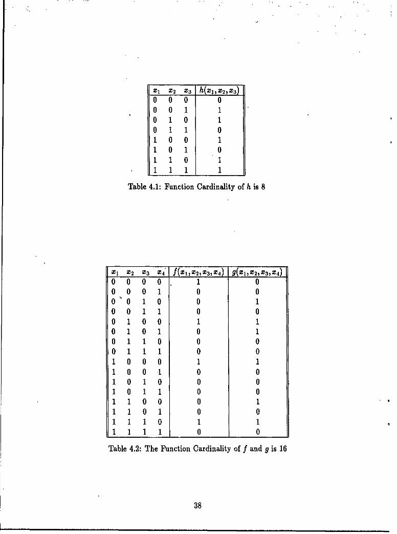
01 02 03 h(xlX2,X3)0 0 0 00 0 1 10 1 0 10 1 1 01 0 0 11 0 1 01 1 0 11 1 1 1

Table 4.1: Function Cardinality of h is 8

-TI -T2 X3 -T4_ f(2:170,1X3,704) g(-Tl,-2, Z3,:4)

0 0 0 0 1 00 0 0 1 0 00 0 1 0 0 10 0 1 1 0 00 1 0 0 1 10 1 0 1 0 10 1 1 0 0 00 1 1 1 0 01 0 0 0 1 11 0 0 1 0 01 0 1 0 0 01 0 1 1 0 01 1 0 0 0 1

1 1 0 1 0 01 11 0 1 1

1111 0 0

Table 4.2: The Function Cardinality of f and g is 16

38

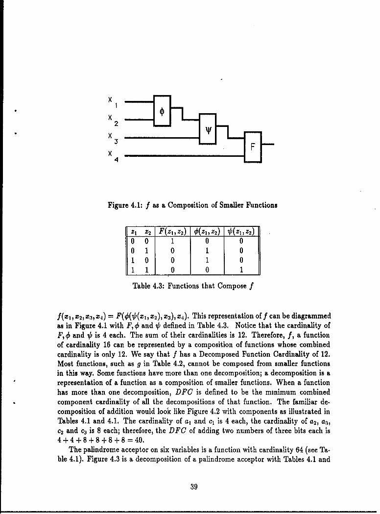
x

x2

x3

x4

Figure 4.1: f as a Composition of Smaller Functions

Zl z2 F(zi,z 2) q(Zl),Z2) __(_iZ2)

0 0 1 0 00 1 0 1 01 0 0 1 011 0 0 1

Table 4.3: Functions that Compose f

f~zl~z X 3, 4) = F(4O(4(zi, X2), ), X x4 ). This representation of f can be diagrammedas in Figure 4.1 with F, O and Ob defined in Table 4.3. Notice that the cardinality ofF, s0 and b is 4 each. The sum of their cardinalities is 12. Therefore, f, a functionof cardinality 16 can be represented by a composition of functions whose combinedcardinality is only 12. We say that f has a Decomposed Function Cardinality of 12.Most functions, such as g in Table 4.2, cannot be composed from smaller functionsin this way. Some functions have more than one decomposition; a decomposition is arepresentation of a function as a composition of smaller functions. When a functionhas more than one decomposition, DFC is defined to be the minimum combinedcomponent cardinality of all the decompositions of that function. The familiar de-composition of addition would look like Figure 4.2 with components as illustrated inTables 4.1 and 4.1. The cardinality of a, and Cl is 4 each, the cardinality of a2, a3 ,c2 and c3 is 8 each; therefore, the DFC of adding two numbers of three bits each is4+4+8+8+8+8 =40.

The palindrome acceptor on six variables is a function with cardinality 64 (see Ta-ble 4.1). Figure 4.3 is a decomposition of a palindrome acceptor with Tables 4.1 and

39

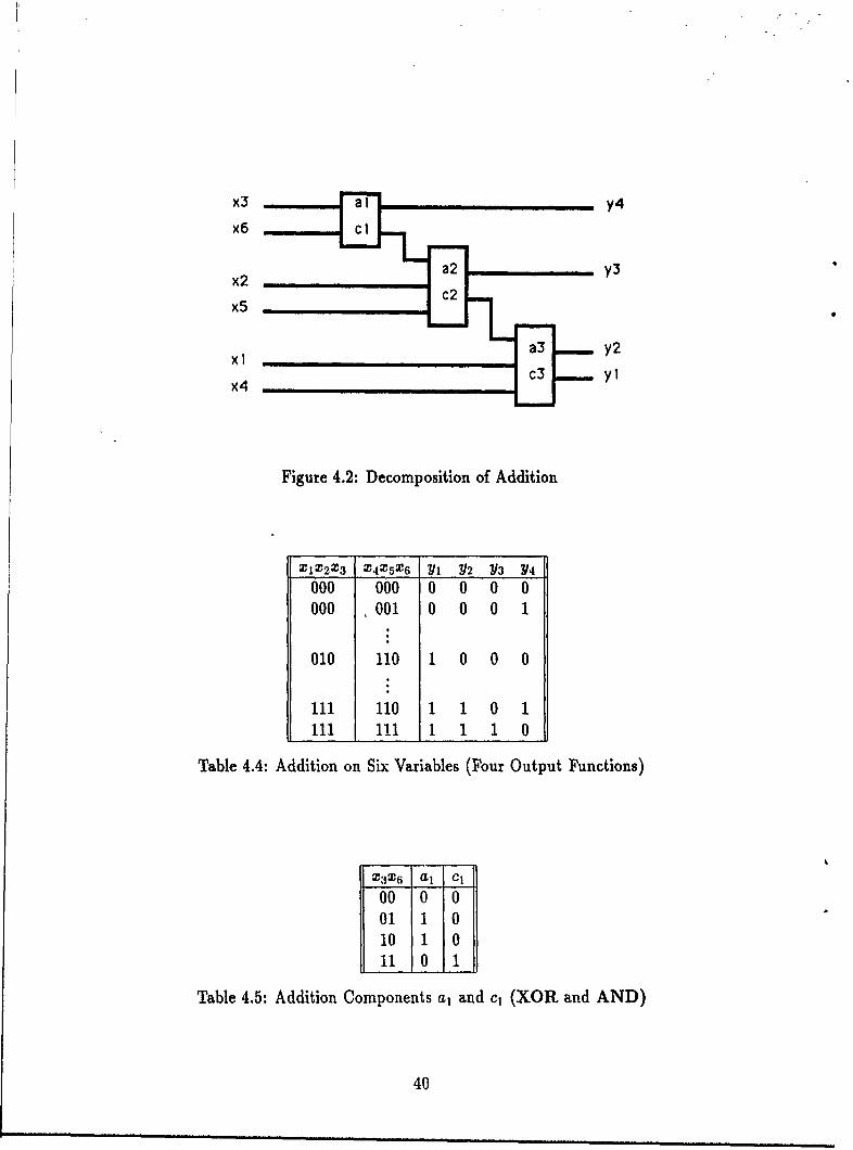
X3 aIy4

x 6a y3

x5

x4 c

Figure 4.2: Decomposition of Addition

X1X2X 3 X4X5X6 YI Y2 Y3 Y/4

000 000 0 0 0 0000 ~001 0 0 0 1

010 110 1 0 0 0

1l1 110 1 1 0 1il1 111 1 1 1 0

Table 4.4: Addition on Six Variables (Four Output Functions)

X3 X6 a, C,00 001 1 0110) 1 0

11 0 11Table 4.5: Addition Components a, and c, (XOR an~d AND)

40

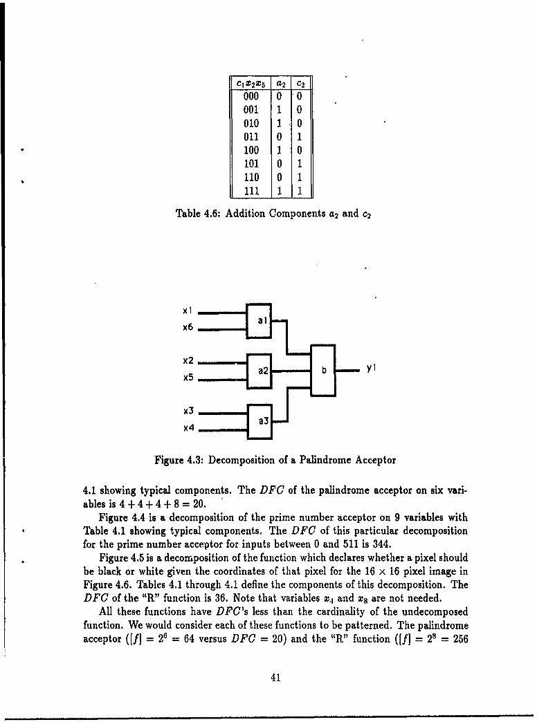
CI X 2 X5 a 2 c 2

000 0 0001 1 0010 1 0011 0 1100 1 0

101 0 1110 0 1111 1 I

Table 4.6: Addition Components a2 and c2

Xlx6

x2

x5

X3

x4

Figure 4.3: Decomposition of a Palindrome Acceptor

4.1 showing typical components. The DFC of the palindrome acceptor on six vari-ables is 4 + 4 + 4 + 8 = 20.

Figure 4.4 is a decomposition of the prime number acceptor on 9 variables withTable 4.1 showing typical components. The DFC of this particular decompositionfor the prime number acceptor for inputs between 0 and 511 is 344.

Figure 4.5 is a decomposition of the function which declares whether a pixel shouldbe black or white given the coordinates of that pixel for the 16 x 16 pixel image inFigure 4.6. Tables 4.1 through 4.1 define the components of this decomposition. TheDFC of the "R" function is 36. Note that variables x., and x are not needed.

All these functions have DFC's less than the cardinality of the undecomposedfunction. We would consider each of these functions to be patterned. The palindromeacceptor (If] = 26 - 64 versus DFC = 20) and the "R" function ([fJ = 28 = 256

41

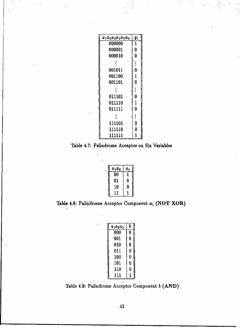
X1X 2 X3 X4 X5 X 6 YI

000000 1000001 0

000010 0

001011 0001100 1001101 0

011101 0011110 1011111 0

111101 0111110 0111111 1

Table 4.7: Palindrome Acceptor on Six Variables

100 1101 010 0

11001

Table 4.8: Palindrome Acceptor Component a, (NOT XOR)

a1a 2a3 b000 0001 0010 0011 0100 0101 0110 0111 1

Table 4.9: Palindrome Acceptor Component b (AND)

42

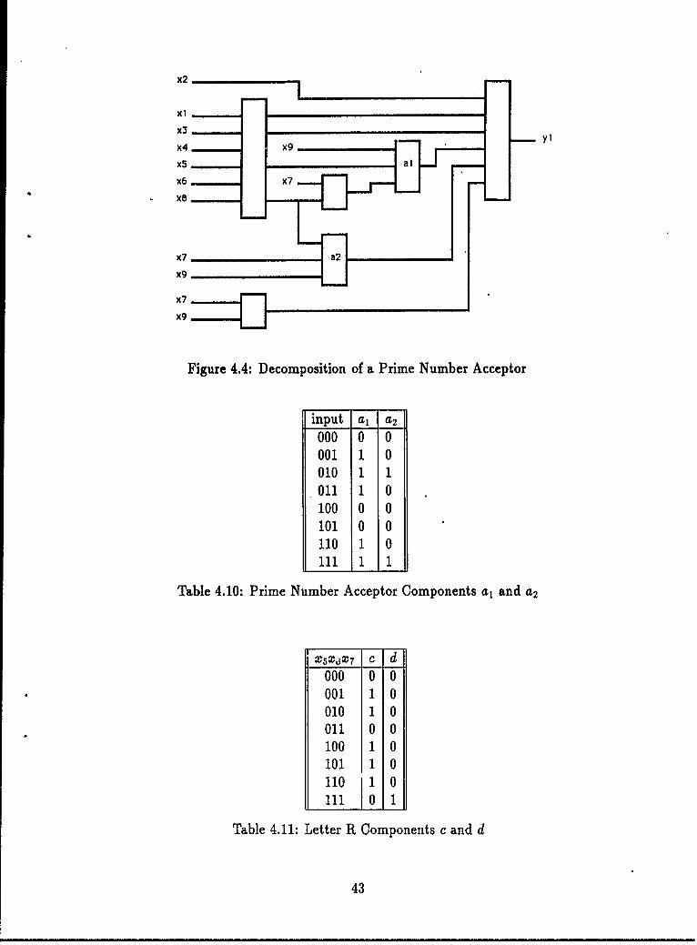
x2

X5 al

x65

q - X8

07 _____________

X9

07

X9

Figure 4.4: Decomposition of a Prime Number Acceptor

input a, a2

000 0 0001 1 0010 1 1011 1 0100 0 0101 0 0110 1 0111 1 1

Table 4.10: Prime Number Acceptor Components a, and a2

X5X,3X7 c d000 0 0

*0011 0010 1 0011 0 0100 1 0101 1 0110 1 10ill 0

Table 4.11: Letter R Components c and d

43

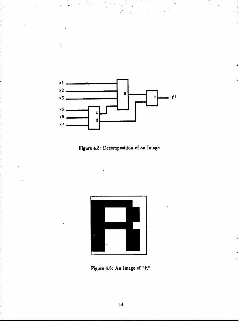
x2 _____________

'(3 y__ _ _ _ _ _ _ _ _ _

'(5

X60(

Figure 4.5: Decomposition of an Image

Figure 4.6: An Image of "IV'

44

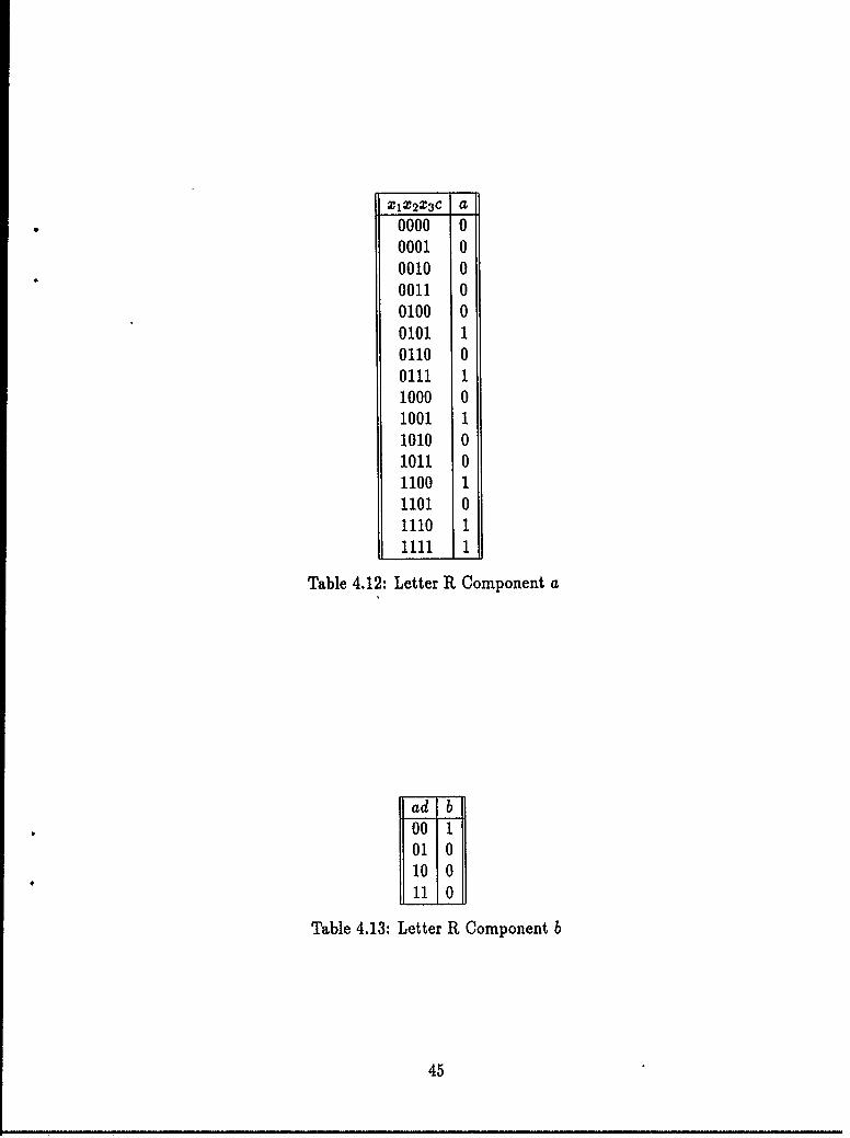
XIX,2a 3c a*0000 0

0001 00010 00011 00100 00101 10110 00111 11000 01001 11010 01011 01100 11101 01110 11111 1

Table 4.12: Letter R Component a

ad*0 0

0110

Table 4.13: Letter Rt Component b

45

versus DFC = 36) are very patterned, while the prime number acceptor ([f] = 29 -512 versus DFC = 344) is only slightly patterned.

The components of a decomposition can be any kind of function, not just the usuallogical functions (AND, OR, XOR, etc.). Note also that some of these decompositionsare very familiar (e.g. addition or the palindrome acceptor) while others were notpreviously known (e.g. the primality test or the "').

We believe that DFC is a very robust measure of pattern-ness. As in the previousexamples, where completely different kinds of patterns are involved, a small DFC(compared to the cardinality of the undecomposed function) is truly indicative ofpattern-ness.

The development of DFC began at the Air'Force Institute of Technology (AFIT)where Matthew Kabrisky stressed the fundamental importance of features in recog-nizer design. DFC resulted from an attempt to generalize the geometric patternrecognition concept of "features." We realized that features are just intermediatestages in the data flow that promote a computationaly efficient realization of a func-tion. Function decomposition also produces these intermediate stages of data forexactly the same purpose. DFC allows for an explanation of pattern-ness that coversthe common pattern recognition paradigms, i.e. geometric, syntactic and artificialintelligence approaches [49'. It seems that the one common factor in all these ap-proaches was this decomposition idea. The idea gained further credence when werealized that the "Divide and Conquer" approach to algorithm design is essentially afunction decomposition approach. We were eventually directed 2 to some theoreticaldevelopments of function decomposition in the Switching Theory literature. Hereagain is this idea in yet another context.

In addition to these informal arguments for the robustness of DFC as a measureof pattern-ness there are several more objective supporting arguments. Chapter 6empirically relates DFC to factors in data compression and to complexity as ratedby people. The remainder of this chapter will report on the relationship betweenDFC and three of the most common measures of computational complexity. Firstwe consider program length. By treating DFC as a component of program length wecan apply some useful results from Information Theory (see [12, 23)). We then relateDFC to time complexity. Under reasonable assumptions one can prove that a smalltime complexity implies a small DFC (see [54]). Finally, we point out that DFC is aspecial case of circuit size complexity. By connecting DFC to these traditional mea-sures (i.e. program length, time complexity and circuit size complexity) we supportthe contention that DFC is a reflection of a very general property, as we would hopewould be the case for a measure of pattern-ness.

2By Frank Brown of AFIT.

46

4.2 Decomposed Function Cardinality

We need a more formal notation for the representation of a function's decompositionto define Decomposed Function Cardinality (DFC). For f : X1 x X 2 x... x X, -4 Y, arepresentation r! of f is a finite, acyclic, directed graph G and a set of finite functionsP. 'That is, r! = (G, P). G and P are defined below.

It will simplify the notation if we rename some sets. We will use Ui to representinput (Xj), intermediate (Z4), and output (Y) sets. In particular, let

IXi i = 1, 2, ....

Ui = Zi-, i = n+1, n+2, ..., n+[P]-1Y i= n+[P].

In this notation,f:U 1 XU 2 X ... X Un -- Un+[p],

and U,+1, U,+2 ,... Un+fp]-i are the intermediate ("feature") sets that are created asa result of the decomposition.

The graph (G) consists of a set of vertices (V) and a set of arcs (A). That is,G = (V, A). There is a vertex in the graph for each variable in the representation,i.e. V = {uI,u 2,. .. ,u,+[p}. The lower case ui is a variable for the set Uj. A is asubset of V x V, called a set of arcs. Indegree of ui is 0 for i = 1,2,... ,n; outdegreeof un+(p] is 0; indegree of un+P] is 1; indegree and outdegree of ui are not 0 fori = n+ 1,n+2,...,n+ [P]- 1.

P = {PhP2,... ,P[P} is a set of nonempty and nonconstant functions of the fol-lowing form:

PJ :Xui -4 uJ, =n + 1,n + 2,...,n + [P],

iE j

where Ij is a set of the indices of the input variables for pj. That is, with I the set ofpositive integers,

Ij = {i E I I (ui,u ) E A}.

A and P are such that (ui, uj) E A if and only if there exists a pj E P which hasi E Ij. Let nj be the number of variables input to pj. That is, nj = [I].

In summary,rf= (G,P),G =(V, A),

V = {Ui)U 2, ... ,Un+[PJ},

AC V xV,

P = {PHP2,... ,P(P},

andP: T i _ j

E7tj

47

DFC (c.f. [48, pp.37-481: ) is used with two meanings. First, it is used to denotethe DFC of a particular representation of function,

[P]DFC( r) = Z(llEUj]).

j=1 iEzj

When U, = {0,1} for all j, this becomes:

[P]DFC(rf) - 2".

j=1

We are occasionally interested in using the actual cardinality [pj] of the componentfunctions rather than 2"j . We call this Decomposed Partial Function Cardinality(DPFC),

(P]DPFC(rf) = [pj].

j=1

When all the component functions of a representation are total the two measuresDFC and DPFC are the same.

When we talk about the DFC of a function, we mean the DFC of that function'soptimal representation. If 7R is the set of all possible representations then

DFC(f) = minimum over rf E 1 of (DFC(rf)).

The DPFC of a function is similarly defined. We also use simply DFC (or DPFC)when the particular function or representation is made clear by the context.

4.3 Decompositions Encoded as Programs

4.3.1 Introduction

We want to relate DFC to program length as developed in Appendix A. In partic-ular, we want to formalize how representations of decompositions are special casesof programs. The cost function on representations that then corresponds to pro-gram length is of special interest since we know a number of properties of programlength. We must also address the concern that a decomposition of a function consistsof both component functions and their interconnections while DFC only measuresthe complexity of the component functions. After all, it could be the case that thecomplexity of the interconnections is independently important in the true measure ofpattern-ness.

We will be concerned with a binary function f:{O, 1}" -+ {0, 1} and representationsof such functions denoted rf. We will also be interested in the optimal representation

'In the notation of [481, DFC is exactly fr(r,-opt) when w(r) = 1 for all r in R' and R' is theset of all Boolean functions of the form f : {O, 1}n --+ {O, 1}"' , m and n1 positive integers.

48

of a given function f which will be denoted Rf. Let A* denote the set of all finitestrings from alphabet A. Define an encoding procedure e : -4 {0, 1}*, where R isthe set of all possible representations. We prove that e(rf) is a program in the formalsense of Appendix A. We define a cost function on encodings as simply their stringlength, L(e(rf)). L is like a combinational form of Kolmogorov complexity and hasmany of its properties (see [33] and [54, Section 5.7]). We use the relationships ofAppendix A to prove a number of properties of e. In particular we prove that for allf 2(n, + 1) < L(e(Rf)) < 2"n + 1,

there exists a function f such that

L(e(Rf)) = 2" + 1,

and that2n < average (L(e(Rf))) < 2" + 1.

With respect to the concern that DFC does not reflect the interconnection complexity,we prove that if DFC is small then L(e(Rj)) (which does reflect interconnectioncomplexity) is also small.

4.3.2 Encoding Procedure

We now define a method for encoding decompositions into binary strings. The en-coding procedure produces a binary string e(rf) which is an identifier of a uniquefunction of the form f: {0,1}" {O, 1}. The procedure for generating encodings isdefined on RV, a subset of R. In particular, using the notation of Section 4.2, RV isthe subset of R such that:

1. IF] < 2",

2. (pi -< 2" for i = 1, 2,...,e]

3. [A] < 2".

We will prove that although VI is a proper subset of 1R, RI includes all optimalrepresentations. We use the notation ra] to specify the smallest integer that is greaterthan or equal to the real number a. Similarly, La] is the largest integer less than orequal to a. There is one other relationship which is a direct consequence of 1 above.

Theorem 4.1 For any r1 in R' an arc in A can be specified with n 2 bits for n > 4.

Proof:By definition of V, [V] < (n+[P]). Thus, a vi in V can be specified with rlog(n+ [P])]bits (log to the base 2). By constraint 1 on 7V', [log(n + [P])] < rlog(n + 2")] <rn log(n)]. Finally, since an arc can be defined by its head and tail vertices, an arccan be specified with 2[rnlog(n)] bits, which is less than or equal to n 2 for n > 4.1

49

The objective of the following encoding scheme is to encode any reasonable rfinto as short a binary string as possible while keeping a manageable expression forL(e(rf)). We assume that n is known. If n is not known, a unary representation of nusing n + 1 bits could be added to the front of the encoding. The encoding- assumesthat all functions involved are total. If a partial function is involved, it can be madetotal by arbitrarily assigning all Don't-Cares to be 0. The encoding procedure is asfollows:

1. The first bit of e(ri)) indicates whether or not the function is decomposed.When this bit is 0, the function is not decomposed and the rest of the programlists, in the order of the domain of f, all the images of f. When this bit is 1the rest of the encoding is as follows.

2. The next n bits specify [P], which is possible -by the first constraint on V'.

3. If [P] is zero then f is either a constant or a projection of one of its variables.When [P] is zero the next n + 1 bits of the encoding indicate which constantor projection function. If f is a projection of the ijh variable then the ijh ofthe first n bits is one and the others are zero. If f is a constant, which willbe indicated by the first n bits being all zero, then the n + 11h bit indicateswhich constant function is f. The total encoding of any constant or projectionfunction therefore requires 2(n + 1) bits. If f is not a constant or projectionfunction then [P] is not zero-and the encoding proceeds as follows.

4. The encoding repeats the following for i = 1 ... [P]

a. The first n bits specify [Pi], which is possible by the second constraint on R'.

b. The next [pi] bits specify pi.

5. The next n bits of the program specify [A], which is possible by the thirdconstraint on '.

6. The encoding then repeats the following for i = 1 ... [A]. The ith arc is specifiedby n 2 bits, which is possible by Theorem 4.1.

4.3.3 Length of an Encoding

We now develop the expression for the length of the string which results from theencoding procedure.

Theorem 4.2 If[P] = 0 then L(e(rf)) = 2(n+ 1); if [P] = 1 then L(e(r)) 1+ 2";otherwise L(e(rf)) = 1 + 2n + n2[A] + niP] + DFC(f).

50

Proof:When [P) = 0 there is the bit of step 1, the n bits of step 2 and the n + 1 bits of step3. When [P] = 1, the worst case is when there are no vacuous variables and thenthere is the bit of step 1 and the 2n bits of f. Otherwise: Step 1 uses 1 bit. Step 2uses n bits. Step 4 uses a sum as i = 1, 2,..., [P] of the bits required for part a) plusthe bits required for part b). Part a) requires n bits. Part b) requires [Pd] bits. Thetotal number of bits required for Step 4 then is:

[P] IP]

E(n + [pi) = n[P] + -pi] = n[P] + DFC(f).i=1 i=1

Step 5 uses n bits. Step 6 uses a sum as i = 1 to [A] of the bits required for an arc.An arc requires n2 bits, assuming n > 4. The total number of bits required for Step6 then is:

(A)

8=1

Therefore,

L(e(rf)) = 1 + n + n[P] + DFC(f) + n + n 2[A] = 1 + 2n + n2[A] + n[P] + DFC(f).

0

4.3.4 VZ' Includes All Optimal Representations

As mentioned earlier, R' is a proper subset of R ; for example, we could define an r!with arbitrarily many identity functions so [P] would be larger than that allowed forencoding. However, RI includes most reasonable representations and we prove that RIincludes all "optimal" representations. For every f, define re-opt as a representationof f such that L(e(rf-,pj)) <_ L(e(rf)) for all rf that represent f. In order to provethat all optimal representations are in R! we need several results which we developnow.

Theorem 4.3 For n > 3, 2(n + 1) < L(e(rj-oft)) 1 + 2".

Proof:The right inequality follows since an arbitrary f has a representation with [P] = 1(i.e. p = f) and whose length is 1 + 2'. The left inequality follows immediatelyif rf is not a decomposition. If rf is a decomposition then either, L(e(r1 )) =

1 + 2n + n [A] + n[P + DFC(f) 2(n + 1) or L(e(rf)) = 2(n + 1).0)

The DFC of a total function cannot be greater than its cardinality.

Theorem 4.4 DFC(f) 2n.

51

Proof:From Theorem 4.3, L(e(rf-pt)),:_ 1 + 2". By Theorem 4.2, 1 +-2n + n 2[A] + ni[P] +DFC(f) < 1 + 2" or 2n + n2 [A] [+ I[P] + DFC(f) < 2". Since all the terms on theleft are positive, each term is less than or equal to 2n. In particular, DFC(f) < 2".0

No component of a decomposition can be larger than the whole DFC.

Theorem 4.5 [pd 2" fori = 1,2,...,[P].

Proof:From Theorem 4.4, DFC(f) _ 2n. Since all the [pi] terms that sum to DFC(f) arepositive, each term must be less than or equal to 2".0

The number of components cannot exceed the DFC.

Theorem 4.6 [P] < 2".

Proof:n[P] is a term in L(e(rfopt)) by Theorem 4.2 and must be less than or equal to 2n

by Theorem 4.3. Finally, since n > 1 we have [P] 2n.

0

The number of arcs cannot exceed the DFC.

Theorem 4.7 [A] < 2".

Proof:Follows as in Theorem 4.6.0

Finally we can prove that R! -includes all optimal representations.

Theorem 4.8 For all f of the form f : {O, 1}" -- {0, 1}, rfopt E 1V.

Proof:Follows from Theorems 4.5, 4.6, and 4.7 and the definition of 7.'.0

4.3.5 Properties of Encodings

We now can relate the encoded representations to the programs of Appendix A.

Theorem 4.9 e(rf) is a program.

52

Proof:The set of e(rf) for all rf E 7! is a language P satisfying the prefix condition. ForF as the set of all functions of the form f : {0, 1}n, -* {O, 1} define M : P -* F suchthat M(e(rf)) = f. Under these conditions, (P, F, M) form a programmable machineas defined in Appendix A.0

Because e(rf) is a program, all the results about programs apply to e(rf). Wewant to highlight a few of these results in the present context.

Theorem 4.10 There ezists a function f such that L(e(rf-opt)) = 1 + 2n.

Proof:Suppose to the contrary that no such function existed. That is, the worst cost of anyfunction is 2" or less. We know there exist functions with cost strictly less than 2",e.g. a constant function. In this situation the average L(e(rf)) is strictly less than2"; that is, we have an average of a set of finite numbers containing some numbersless than 2" but containing no numbers greater than 2". However, since e(rf) is aprogram the average L(e(rf)) being strictly less than 2" contradicts Theorem A.16.Therefore the supposition is false and the theorem is proven.0

Theorem 4.11 2" < average L(e(rtopj)) < 1 + 2".

Proof:The left inequality follows from Corollary A.3. For the right inequality, we know thatthere exist functions with cost strictly less than 2" + 1, e.g. a constant function, andthat there are no functions with cost greater than 2" + 1 by Theorem 4.3. Thereforethe average L(e(rf)) is strictly less than 2n + 1.0

4.3.6 Decomposed Function Cardinality and Program Length

We are concerned with the question: "How well does DFC(f) capture the essentialcomplexity of a function?" In Appendix A we developed the idea of program lengthas a very general characterization of size complexity. In this section we found thate(rf) is a program with length L(e(rf)) = 1+ 2n+n 2[A]+n[P]+ DFC(f). Therefore,one step in relating DFC(f) to general complexity is to assess its role in L(e(rf)).

In those cases where L(e(rf _op,) = 1 + 2", DFC(f) = [f] = 2" = L(e(rfo,)) - 1.That is, in most cases DFC(f) is almost exactly L(e(r-opt)). When L(e(rfo.p.)) <1 + 2", we do not have as simple a relationship. However, we can prove that DFC(f)is roughly of the same order of complexity as L(e(r-

53

We already know that L(e(rj_,vt)) cannot be small unless DFC(f) is small sinceDFC(f) is a part of L(e(r _opt)). Our concern is that DFC(f)might be small whileL(e(rfo.0 t)) is large. That is, we do not want to think that a function is patternedbased on DFC while it really is not patterned when you consider the full cost ofrepresentation as measured by L(e(rf _opt )). In order to demonstrate that this is nota problem, we will show that L(e(r-opt)) < n3DFC(f). That is, L(e(r _opt)) is neverof a much higher order than DFC(f).'

Theorem 4.12 DFC(f) < L(e(rf _o0 t)) < n3 DFC(f) for all n > 4 andDFG(f) > 1.

Proof-The left inequality follows immediately. For the right, let ni be the number of inputvariables for pi. Then DFC(f) = Ei-1 2n'. Since ni > 2 we have DFC(f) _ 4[P].

Also, [A] = E[__1 n- + 1 and since n, n we have [A] _ n[P] +1. Now use the secondinequality to eliminate [A] from the expression for L(e(rf _op)) to get:

L(e(rf _opt)) _ 1 + 2n + n2(n[P] + 1) + n[P] + DFC(f)

and then use the first inequality to eliminate [P] to get:

L(e(rfo.0 t)) K_ 1 + 2n + n2 (n1DFC(f) + 1) + n1DFC(f) + DFC(f)4 4

or equivalently:

L(e(r _ot)) < 1 + 2n + n2 + -DFC(f)(n3 + n + 4)4

This simplifies to L(e(rj.o.,f)) < n3DFC(f) for n > 4 and DFC(f) > 1.0

From Theorem 4.12 we know that if DFC(f) is small then program length isalso small. For example, if DFC(f) is polynomial in n then program length is alsopolynomial in n. The point is that DFC(f) reflects the essential complexity eventhough it does not directly include a measure of the interconnection complexity of

the representation.There is another indication of the relative importance of interconnection complex-

ity versus DFC. If the interconnections are minimized without regard to DFC thenthe result is n + 1 interconnections (n the number of non-vacuous variables). That is,

all functions on a given number of variables have the same minimum interconnectioncomplexity.

4c.f. [54] Theorem 5.7.5.

54

4.4 Decomposed Function Cardinality and TimeComplexity

Another concern about the DFC(f) measure of pattern-ness is that it is based oncombinational machines. What if there are patterns that only become measurablewith respect to sequential machines? If this were the case then DFC(f) would notmeasure the patterns of interest in most real computing problems. Of course, this isnot the case. In order to demonstrate that DFC(f) will be small whenever there existsa good sequential algorithm, we relate DFC(f) to time complexity (the traditiomalmeasure of Computational Complexity Theory). There are several differences in thetwo perspectives (time complexity versus DFC(f)) that must be considered. Onedifference is that DFC(f) considers complexity in terms of a single measure of awhole finite function while traditional complexity is in terms of a particular inputto an infinite function. A second difference is that Pattern Theory is based on sizecomplexity while traditional measures are based on time complexity. The objectiveof this section is to demonstrate that size and time complexity are simpiy differentperspectives of what might be considered the essential computational complexity ofa function.

Why not just use time complexity in the first place? First and foremost, the timecomplexity of all finite functions is 0(1). Therefore, time complexity does not differ-entiate between patterned and un-patterned finite functions. Another problem withtime complexity is finding out what it is. We know how to find the time complexityof an algorithm. But we do not know whether or not that is the time complexity ofthe function. It may simply be a poor algorithm. This also presupposes that youhave an algorithm for the function, which is begging our question.

Once the relationship between DFC(f) and traditional time complexity is es-tablished we are able to apply results from the traditional theory of computationalcomplexity. Also, because small time complexity implies small DFC(f) we knowthat patterns as measured by time complexity are a subset of patterns as measuredby DFC(f).

Traditional time complexity t(n) is defined in terms of the run-time of a TuringMachine [59] which realizes a function of the form f : {0, 1}* -4 {0, 1}, when theinput is a string of length n. On the other hand, DFC(f) is defined as a measureof a realization of a function of the form g : {0, 1}" --+ {0, 1}. In order to be able tocompare these two measures we use the following device. Let f : {0, 1}* --, {0, 1} bea function and f,: {0, 1}n

_ {0, 1} for n = 0,1,2,... be a sequence of functions suchthat f(x) = f(x) for all x in {0, 1}" and for all n in N. The DFC complexity of arepresentation of f,, is denoted s(n).

We developed this device and the following theorem not knowing that a similarresult had been previously demonstrated (see [19, 55]). However, because this isfundamentally important to Pattern Theory, we want to present a proof. Ratherthan repeating the original proof, we present our proof and suggest that the readersee [64, pp.271-276] for a more elegant demonstration of this result.

55

Theorem 4.13 If f : {,1}* - {0, 1} is a function with an algorithm of worst-casetime complexity t(n) then for every n E N, there exists a combinational realization off, such that s(n) is in O(t(n) log t(n)).

Proof:Let M = {, r, Q, q0, 6, F} be the Turing Machine which realizes f with worst casetime complexity t(n), where r is the tape alphabet, E is a subset of r called theinput alphabet, Q is a set of machine states, q0 is the start state, F is a set of finalstates, and 6 : r x Q --+ r x Q x {-1, +1} is the transition function (reference [59,pp.211-215]). The L (for left) and R (for right) of Sudkamp's definition have beenreplaced with -1 and +1; the reason for this will be pointed out later. We break 6into 6' : r x Q -- , r6" : r x Q -- Q, and 6"': r x Q -- {-1,+1} such that 6(g,q)equals (6'(g, q), 6"(g, q), 6"(g, q)).

Define the interval Z = {0,1,2, ... , t(n)} and the function p : Z -- Z such thatp(i) is the position of the tape after i transitions. Define q : Z - Q such that q(i) isthe state of the machine after i transitions. Define g : Z x Z r P such that g(ij)is the symbol in the jth position of the tape after i transitions. We use p, q, g and hto establish a combinational realization of fn. Define h : on(n) x z x Q -- (n) suchthat g(i,j) = h(g(i - 1,j),p(i - 1),q(i - 1)) for all i and j.

From the starting conditions of the Turing Machine p(O) = 1, q(O) = qo, andg(Oj) = x(j) (i.e. the input) for j = 1,2,... , n. From the final conditions, p(t(n)) = 0and q(t(n)) is the state defined to correspond to f(z) = 0 and f(z) = 1 as appropriate.

By the definition of a Turing Machine we can write difference equations for p, q,and g:

p(i) = p(i - 1) + 6"(g(i - 1,p(i - 1)),q(i - 1)) for i - 1,2,...,t(n). Using

{-1, +1} as the range of 6"', rather than {L, R}, allows this simple addition. Theincrement in cost associated with each i is the cost of addition plus the cost of 6"',i.e. a(+) + s(6"..), since the cost of all the other functions are accounted for elsewhere.The cost of "" is O(m) (reference [7] where, since the largest number to be addedis t(n),m = log t(n). That is, s(+) = klogt(n). For 6' : r x Q - {-1,+1},we have s(6"') = [rl[Qlog[{-1,+1}] = [r][Q] = k, k some constant. Therefore,s(p) = k1 log(t(n)) + k2.

q(i) = 6"(g(i - 1,p(i - 1)),q(i- 1)), for i = 1,2,... ,t(n). The increment in costassociated with each i is s(6"), since the cost of all the other functions are accountedfor elsewhere. For 6" : F x Q --, Q, we have s(6") = [r][Q]log(Q] = k, k someconstant. Therefore, s(q) = k.

g(i,j) is unchanged for all j except j = p(i- 1) and g(i,p(i- 1)) = 6'(g(i- 1,p(i-1)), q(i - 1)). That is, g(i,j) = h(g(i - 1,j),p(i - 1), q(i - 1)) = .NOT.(.EQ.(j,p(i -1))) x g(i - 1,j) + .EQ.(j,p(i - 1)) x S'(g(i - 1,j),q(i - 1)), where the functions.NOT. and .EQ. are the obviouq logical operators with values 0 or 1 and + and xare arithmetic operators. The increment in cost associated with h is s(.NOT.) +s(+) + s(6') + 2s(.EQ.) + 2s(x). The multiplications always involve a zero or aone, therefore we assume that s(x) is constant. The addition always involves a zero,therefore we assume s(+) is constant. The cost of the logical operators is constant.

56

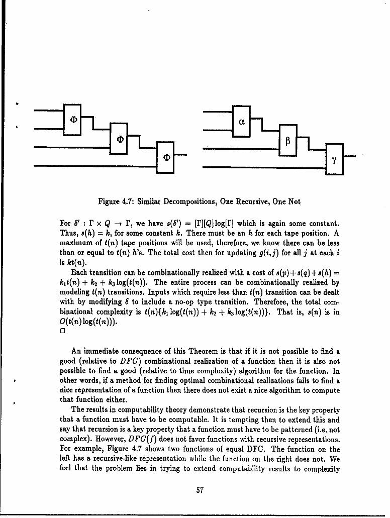
Figure 4.7: Similar Decompositions, One Recursive, One Not

For 6':• r x Q r~1, we have s(6') = [r][Q]log(r] which is again some constant.Thus, s(h) = k, for some constant k. There must be an h for each tape position. A

maximum of t(n) tape positions will be used, therefore, we know there can be lessthan or equal to t(n) h's. The total cost then for updating g(i,j) for all j at each iis kt(n).

Each transition can be combinationally realized with a cost of s(p) + i(q) + s(h) =kit(n) + k2 + k3 log(t(n)). The entire process can be combinationally realized bymodeling t(n) transitions. Inputs which require less than t(n) transition can be dealt

with by modifying 6 to include a no.op type transition. Therefore, the total com-binational complexity is t(n){ki log(t(n)) + k2 + k3 log(t(n))}. That is, s(n) is inO(t(n) log(t(n))).

An immediate consequence of this Theorem is that if it is not possible to find agood (relative to DFC) combinational realization of a function then it is also notpossible to find a good (relative to time complexity) algorithm for the function. Inother words, if a method for finding optimal combinational realizations fails to find anice representation of a function then there does not exist a nice algorithm to computethat function either.

The results in computability theory demonstrate that recursion is the key propertythat a function must have to be computable. It is tempting then to extend this andsay that recursion is a key property that a function must have to be patterned (i.e. notcomplex). However, DFC(f) does not favor functions with recursive representations.For example, Figure 4.7 shows two functions of equal DFC. The function on theleft has a recursive-like representation while the function on the right does not. Wefeel that the problem lies in trying to extend computability results to complexity

57

rather than in DFC(f). Recursion is important in getting finite representations ofinfinite functions (see Appendix A); however, it is not crucial to the complexity offinite functions. There is a real cost savings in recursively reusing components of acomposition; however, we believe that this is a secondary effect and it is not indicativeof the existence or absence of patterns. It would be easy to redefine DFC to reflectthe economy of reusing functions in a composition; for example, we could include onlythe unique pi's in adding up DFC. However, finding this newly defined DFC wouldbe much more difficult. We feel that this improvement in generality is not worth theloss in tractability.

In summary, it has been proven that if a function has low time complexity thenit also has low DFC. This means that if a function has, a nice representation usingsequential constructs (do-while, recursion, etc.) then it also has a nice combinationalrepresentation. The main point is that there is no loss in generality due to the PT 1restriction to combinational machines.

4.5 Decomposed Function Cardinality and Cir-cuit Complexity

There has been a great deal of theoretical work on measuring and minimizing thecomplexity of electronic circuits. Using Savage'76 [541 as the principal reference, wereview the several measures of complexity. "Combinational" complexity is the num-ber of circuit elements required to realize a function. "Formula size" is the numberof operators in an algebraic expression of the function. "Delay complexity" is thelength of the longest path from input to output in a realization of a function. Combi-national complexity is very similar to Decomposed Function Cardinality (DFC). Wewill discuss their relationship first. The relationship of combinational complexity toformula size and depth complexity is then summarized from Savage'76.

Combinational complexity in Savage'76 is defined relative to a set of basis func-tions (Q). A given Boolean function f is then realized by combinations of the elementsof Q. The combinational complexity Cn(f) of a Boolean function f relative to thebasis 11 is the minimum number of elements from 0 required to realize f.

Cn(f) is sometimes generalized by allowing the various elements of f1 to havedifferent costs [52]. For example, we could define a weighting function (w : 1 -4 R,7?. the real numbers) on Q. Then the generalized cost of a function (Cn, (f)) is thesum of the weights of the elements in the realization that minimizes that sum. CO(f)is the special case of Co, (f) where w is the constant 1 function.

DFC is also a special case of this generalized combinational complexity. DFC isexactly Cnj,,(f) when Q is the set of all Boolean functions and w(p) = [p] for all p E ft.

Note that for the most common set of basis functions, Q = {AND, OR, NOT},Cp(f) and DFC are also very similar.

Theorem 4.14 For a Boolean function f and basis set Q = {AND, OR, NOT},DFC(f) 4Cg(f) < 4nDFC(f).

58

Proof:DFC < 4Cn since each element of fZ has cardinality of 4 or less. Suppose the decom-

position of f with minimum DFC is made up of PIi P2, '" ,pp and the number of vari-

ables going into pi is ni. In this case, DFC(f) = i 2. Now, Cr(f) _< E!'I Ci(p,).Since each pi has a sum-of-products representation, we have Cn(pj) _ ni2i[54, p.19].Therefore, Cn(f) E I h2" n = 2< ' = nDFC(f).

0

In summary, CQ is in some ways more general than DFC; but, it is more generalin a way that denies any absolute meaning to complexity. That is, for all functionsf there exist an 12 (n.nely any Q with f as an element) such that Cn(f) = 1. Thisrelativity of complexity to a chosen basis is believed by some to be unavoidable.'The main idea of Pattern Theory is that there is some general absolute measure ofcomplexity in the sense of patterns.

C{AND,ORNOT} is quantitatively similar to DFC but it leads you to artificiallydecompose (i.e. represent in some normal form) un-patterned functions. In PatternTheory, all functions have themselves as a normal form representation. Also, onsmaller functions it gives an artificial importance to members of n.

Savage'76 has little to say about the relationship of combinational complexity toformula size and depth complexity. Depth complexity is proportional to the logarithmof Co. Also, Co < formula size. Other than that, not much is known about therelationship between combinational complexity, depth complexity and formula size.

4.6 Summary

This chapter defines our chosen figure-of-merit for algorithm design: DecomposedFunction Cardinality (DFC). We then support the idea that DFC reflects the essentialpattern-ness of a function. Chapter 6 has the results of many experiments thatsupport this idea. In this chapter we supported this idea by showing that if a functionhas an interesting pattern by most other measures then it also has a pattern accordingto DFC. We considered three other measures of computational complexity: programlength, time complexity and circuit complexity.

Appendix A interprets a result from Communications Theory in terms of programsand the length of a program (essentially the number of characters in a listing of aprogram). It turns out that a similar interpretation had previously been made [12].We then related DFC and program length. This relation supports the use of DFCrather than program length as our measure of patterns because DFC is more tractableand yet reflects the essential complexity that program length would measure.

We developed a formal proof of the relationship between DFC and time complexity.It turns out that this relationship had also been previously demonstrated [54]. Therelationship between DFC and time complexity demonstrates that DFC is a moregeneral measure of complexity (that is, anything patterned relative to time complexitywill also be patterned relative to DFC). DFC also has the advantage over time

59

complexity in that it is meaningful for finite functions and allows for a method ofdesign (Chapter 5).

The relationship between DFC and circuit complexity is quite simple. DFC is aspecial case of the more general definition of circuit complexity. We believe it is thespecial case that reflects the essential pattern-ness of a function.

We mentioned earlier that it would be desirable to include the cost of the intercon-nections in a general measure of patterns, as in the program length of an encoding of adecomposition. It would also be desirable for a general measure to reflect the savingsof reusing components, as in a recursive representation. However, we believe thatDFC allows you to determine the basic degree of pattern-ness without the complexityof dealing with these secondary effects.

60

Chapter 5

Function Decomposition

5.1 Introduction

By a "function" we mean the traditional mathematical function; that is, a functionis an association between inputs and outputs such that for every input X there isexactly one output f(x). Functions in general may have several inputs, e.g. f(z, y, z).The decomposition of a function is an expression of that function in terms of a com-position of other (usually smaller) functions. For example, if f(XI, X2,... , XS) =

F[A[O(a;1,Z 2), O(X3, X4), (X5, X6)], C(X7, Xs)J then the right-hand side of the equationis a decomposition of the function f. The process of finding a decomposition of afunction is called function decomposition.

Function decomposition is of practical importance in the design of computationalsystems. The realization of a large function in terms of smaller functions has a numberof practical benefits, especially simplifying the design process and lowering the cost ofthe overall realization. The development of function decomposition theory has beenmotivated primarily by Switching (or Logic) Circuit Design, where the lowest levelsub-functions are realized by some standard circuit component (e.g. an AND gate).Pattern Theory holds that function decomposition is of fundamental importance inthe development of all computing systems, including algorithm design and machinelearning. Aside from the practical motivation, function decomposition is a well definedand very interesting mathematical problem.

This chapter has three main sections. Section 5.2 introduces and formally provesthe test for decomposability. The next section describes the Ada trogram used inthis project to decompose functions. The final section reports on performance testsof various versions of the Ada program.

61

5.2 The Basic Decomposition Condition

5.2.1 Introduction

A number of algorithms have been developed to find the decompositions of a givenfunction. All these algorithms are iterative. That is, they decompose the functionin a series of similar steps. The first step decomposes the function into a smallnumber of sub-functions. The second step decomposes each of these sub-functionsinto a small number of sub-subfunctions. This process is repeated until the remainingfunctions are no longer decomposable. The function decomposition algorithms usea fairly standard test for whether or not a function (or sub-function) decomposes.This test is based on what we call the basic decomposition condition. On the otherhand, the function decomposition algorithms use different methods for searching andselecting among possible decompositions. An optimal method of search and selection(other than exhaustive search) has not been defined. The basic decomposition isthe common non-heuristic portion of these algorithms. The basic decompositioncondition test is an exponentially (relative to the number of variables in the function)difficult problem. The number of variable partitions is another exponential factor,however, this factor can perhaps be mitigated with reasonable search heuristics. Thenature of the decomposition test is such that there is no way to limit its exponentialcomplexity. Therefore, the decomposition test is also important as a limiting factorin the practicality of any algorithm which exactly decomposes total functions.

The purpose of this section is to develop a concise, yet rigorous statement of ageneral basic decomposition condition. Many of the previously published statementsof the basic decomposition condition have shortcomings in rigor, generality, or inrequiring an extensive background in non-essential materials. For example, the bibleof function decomposition is the text by H. A. Curtis [14]. However, its not untilpage 471 that the most general form of the decomposition condition is given and anunderstanding of much of the previous 470 pages is required to understand page 471.Reference [14 also does not prove the most general statement of the decompositioncondition, rather it is an extension of the proofs of less general forms, The mostgeneral form given in [141 is also not applicable to multi-valued functions. Finally,[14] has been out of print for some time and it is very difficult to find.

5.2.2 An Intuitive Introduction to the Decomposition Con-dition

Consider a function of the form f : X, x X 2 x ... x X,, - Y. This function isalso denoted f(X1,X 2 ,... , ,,), where x, represents some unspecified value of Xi.1 2,. . . , ,} is called the set of variables of f. We are interested in a partition ofthe variables of f into two sets. A partition is a collection of subsets whose union isthe whole set and whose intersections are all empty. We denote the two sets of vari-ables v, and v2. Therefore, Vl Uv 2 = {X1 , 2,... , ,,} and vl nv 2 = 0. For example, if

62

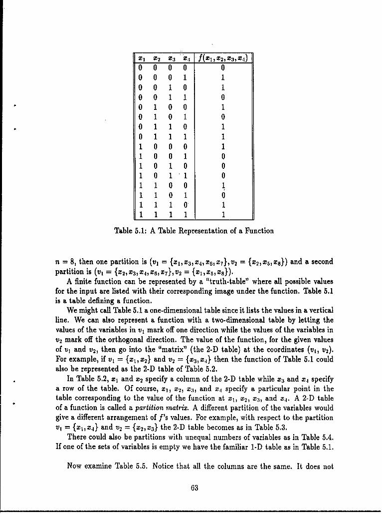
X1 I2 X3 J X7 f X2,1X3,iZ.1)

0 0 0 0 00 0 0 1 10 0 1 0 10 0 1 1 00 1 0 0 10 1 0 1 00 1 1 0

0 1 1 11 0 0 0 11 0 0 1 01 0 1 0 01 0 1 1 0S1 00 1

1 1 0 1 01110 1

I1 111 1

Table 5.1: A Table Representation of a Function

n = 8, then one partition is (v1 = {XlX 3 , 4 ,XX 7},V 2 = {X2 ,2zs, xs}) and a secondpartition is (vI = {X2 ,X 3 ,X, X 6,X 7 },V 2 = {x 1 ,) 5 ,xS}).

A finite function can be represented by a "truth-table" where all possible valuesfor the input are listed with their corresponding image under the function. Table 5.1is a table defining a function.

We might call Table 5.1 a one-dimensional table since it lists the values in a verticalline. We can also represent a function with a two-dimensional table by letting thevalues of the variables in v, mark off one direction while the values of the variables inv2 mark off the orthogonal direction. The value of the function, for the given valuesof v, and v 2, then go into the "matrix" (the 2-D table) at the coordinates (vI, v2).For example, if v, = {X1 ,X 2} and v2 = {X3, X} then the function of Table 5.1 couldalso be represented as the 2-D table of Table 5.2.

In Table 5.2, x, and X2 specify a column of the 2-D table while X3 and x., specifya row of the table. Of course, xj, X2, x3 , and X4 specify a particular point in thetable corresponding to the value of the function at x1, X2, X3 , and X4. A 2-D tableof a function is called a partition matrix. A different partition of the variables wouldgive a different arrangement of f's values. For example, with respect to the partitionV1 = {X,X 4} and v2 = {X2,X 3} the 2-D table becomes as in Table 5.3.

There could also be partitions with unequal numbers of variables as in Table 5.4.If one of the sets of variables is empty we have the familiar 1-D table as in Table 5.1.

Now examine Table 5.5. Notice that all the columns are the same. It does not

63

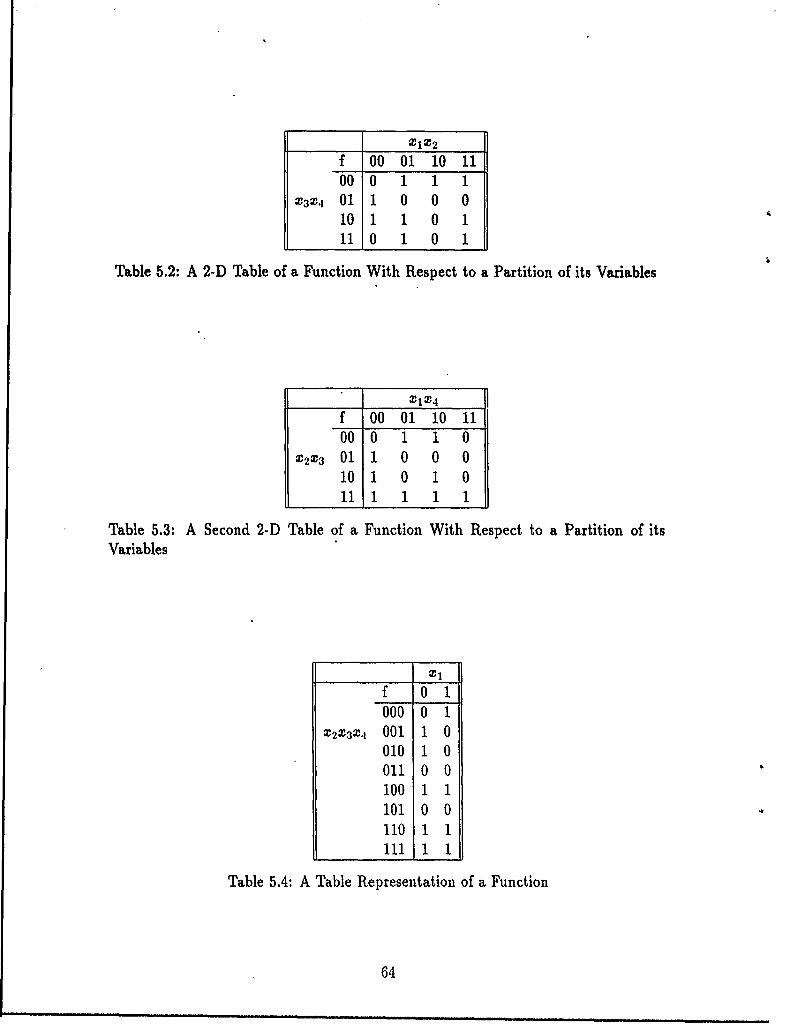
XlM2

f 00 01 10 1100 0 1 1 1

X3X4 01 1 0 0 0

10 1 1 0 111 0 1 0 1

Table 5.2: A 2-D Table of a Function With Respect to a Partition of its Variables

X1X4

f 00 01 10 1100 0 1 1 0

X2X3 01 1 0 0 010 1 0 1 011 1 1 1 1

Table 5.3: A Second 2-D Table of a Function With Respect to a Partition of itsVariables

f 0 1000 0 1

X2X3X 4 001 1 0

010 1 0011 0 0100 1 1101 0 0110 1 1

Table 5.4: A Table Representation of a Function

64

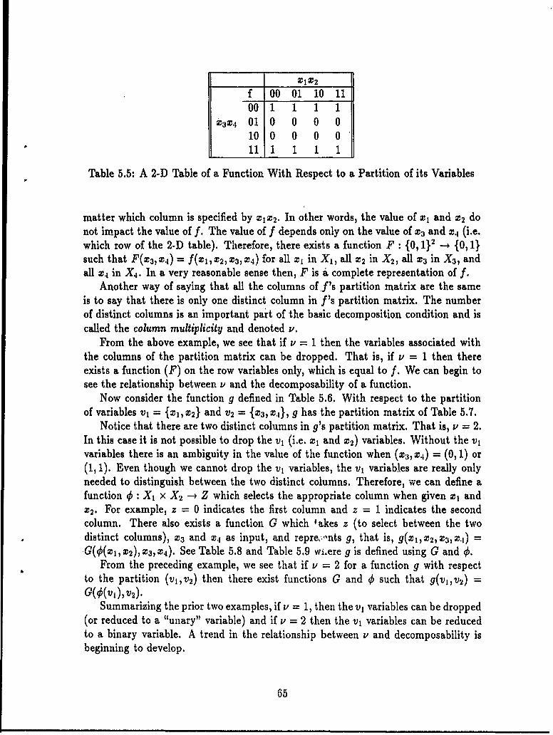
XlX2

f 00 01 10 1100 1 1 1 1

i02 4 01 0 0 0 0

10 0 0 0 011 1 1 1 1

Table 5.5: A 2-D Table of a Function With Respect to a Partition of its Variables

matter which column is specified by ZaX2. In other words, the value of x, and X2 donot impact the value of f. The value of f depends only on the value of X3 and X4 (i.e.which row of the 2-D table). Therefore, there exists a function F : {0, 1}2 + {0,1}such that F(X3 , Z4 ) = f(X1,Z 2 , Z3, X4) for all x, in X1, all X2 in X2 , all X3 in X3 , andall X4 in X4. In a very reasonable sense then, F is a complete representation of f.

Another way of saying that all the columns of f's partition matrix are the sameis to say that there is only one distinct column in f's partition matrix. The numberof distinct columns is an important part of the basic decomposition condition and iscalled the column multiplicity and denoted v.

From the above example, we see that if v = 1 then the variables associated withthe columns of the partition matrix can be dropped. That is, if v = 1 then thereexists a function (F) on the row variables only, which is equal to f. We can begin tosee the relationship between v and the decomposability of a function.

Now consider the function g defined in Table 5.6. With respect to the partitionof variables v, = {fX,X 2 } and v2 = {z3, z,}, g has the partition matrix of Table 5.7.

Notice that there are two distinct columns in g's partition matrix. That is, V = 2.In this case it is not possible to drop the v, (i.e. x, and X2) variables. Without the v,variables there is an ambiguity in the value of the function when (XI, Xj) = (0,1) or(1,1). Even though we cannot drop the v, variables, the vi variables are really onlyneeded to distinguish between the two distinct columns. Therefore, we can define afunction 0 : X, x X 2 -, Z which selects the appropriate column when given z, andz 2. For example, z = 0 indicates the first column and z = 1 indicates the secondcolumn. There also exists a function G which 4akes z (to select between the twodistinct columns), x3 and X4 as input, and repre,,.nts g, that is, g(Xl,Z2,X 3 ,X.1) =,G(O(xlX2),X3, X4). See Table 5.8 and Table 5.9 wiere g is defined using G and 0.

From the preceding example, we see that if v = 2 for a function g with respectto the partition (vI,v 2) then there exist functions G and q such that g(vj,v 2) =

G(cb(v1),V2).Summarizing the prior two examples, if v = 1, then the v, variables can be dropped

(or reduced to a "unary" variable) and if v = 2 then the v, variables can be reducedto a binary variable. A trend in the relationship between v and decomposability isbeginning to develop.

65

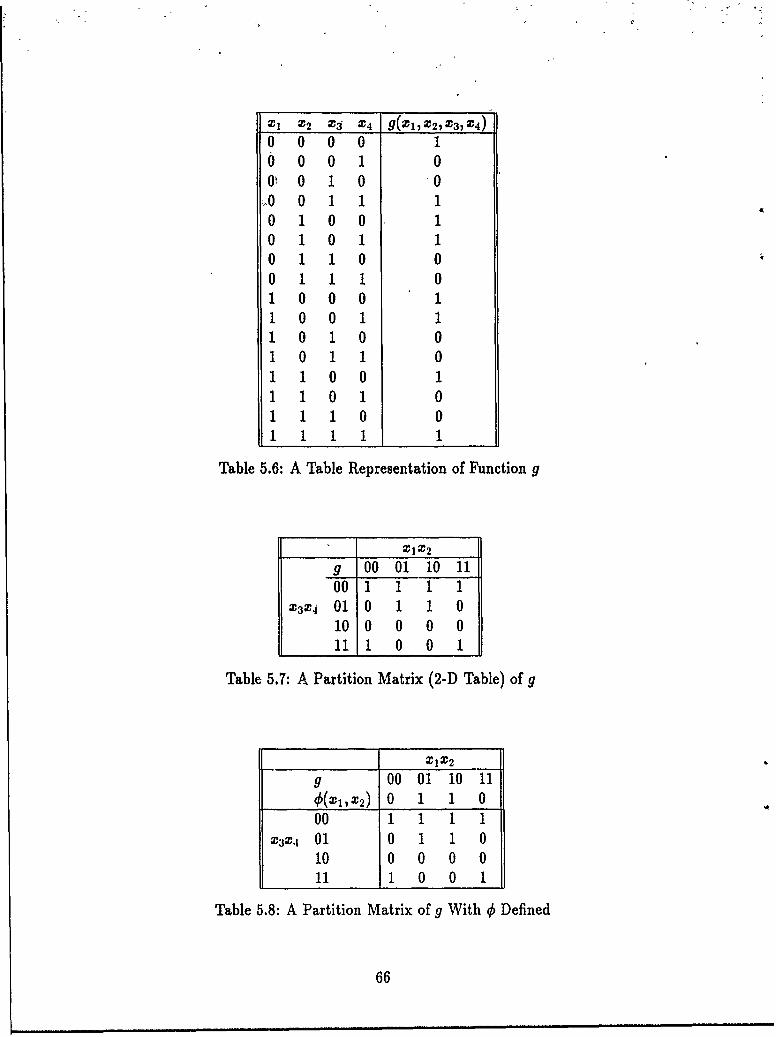
X1 X2 X3 t4 _(____,z3,_4)

0 0 0 0 10 0 1 001 0 1 0 0

1,10 0 1 1 10 1 0 0 10 1 0 1 10 1 1 0 00 1 1 1 01 0 0 01 0 0 11 0 1 0 01 0 1 1 01 1 0 0 11 1 0 1 0

1 0 01 1 11 1

Table 5.6: A Table Representation of Function g

X1lX2

g 00 01 10 1100 1 1 1 1

X3X4 01 0 1 1 010 0 0 0 011 1 0 0 1

Table 5.7: A Partition Matrix (2-D Table) of g

XIX2

g 00 01 10 11O(XI, X2 ) 0 1 1 0

00 1 1 1 1X3X4 01 0 1 1 0

10 0 0 0 011 1 0 0 1

Table 5.8: A Partition Matrix of g With q Defined

66

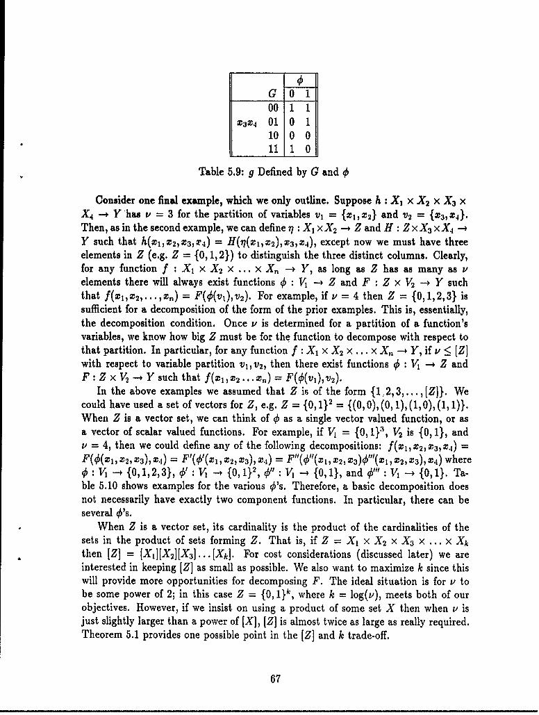
0G 0 1

00 1 1

X3X4 01 0 110 0 0

11 1 0

Table 5.9: g Defined by G and 4

Consider one final example, which we only outline. Suppose h : X, x X 2 x X 3 xX4 --+ Y'has v = 3 for the partition of variables vi = {a 1,X 2} and v2 = IX3,X4}.

Then, as in the second example, we can define 77 : X1 x X 2 -* Z and H : Z x X 3 x X 4 -4

Y such that h(xi, X2,z 3,aX4) = H(n(xl,X 2), X3,X 4), except now we must have threeelements in Z (e.g. Z = {0, 1, 2}) to distinguish the three distinct columns. Clearly,for any function f : X 1 x X 2 x ... x X, -- Y, as long as Z has as many as velements there will always exist functions , : --* Z and F : Z x V2 -4 Y suchthat f(XliX2,...,iX) = F((v 1),v2). For example, if v = 4 then Z = {0,1,2,3} issufficient for a decomposition of the form of the prior examples. This is, essentially,the decomposition condition. Once v is determined for a partition of a function'svariables, we know how big Z must be for the function to decompose with respect tothat partition. In particular, for any function f : X1 x X 2 x ... x X Y, if v < [Z]with respect to variable partition v1,V2, then there exist functions 4, : V1 -+ Z andF: Z x V2 --* Y such that f(XI,2 ...Xn)= F(0(v1),v 2).

In the above examples we assumed that Z is of the form {1, 2,3,...,[Z]}. Wecould have used a set of vectors for Z, e.g. Z = {0, 1}2 = {(0, 0), (0,1), (1, 0), (1, 1)}.When Z is a vector set, we can think of 4 as a single vector valued function, or asa vector of scalar valued functions. For example, if V = {0, 1 1,1, V2 is {0, 1}, andv = 4, then we could define any of the following decompositions: f(XX 2,X 3,X 4) =

F(O(ai, X2 ,X 3 ), .1 ) = F(0'(xi, 2 , X3 ), .) = F"(0I"(X1 ,X 2 ,X 3)0..(X1 ,X 2 ,X 3 ),X 4 ) where4,: V1 - {0,1,2,3}, 0': I __ {0,1}2, 0,": V -+ {0,1}, and 4': V -- {0,1}. Ta-ble 5.10 shows examples for the various O's. Therefore, a basic decomposition doesnot necessarily have exactly two component functions. In particular, there can beseveral O's.

When Z is a vector set, its cardinality is the product of the cardinalities of thesets in the product of sets forming Z. That is, if Z = X, x X 2 x X 3 x ... x Xkthen [Z] = [X1][X 2][X 3 ] ... [XkJ. For cost considerations (discussed later) we areinterested in keeping [Z] as small as possible. We also want to maximize k since thiswill provide more opportunities for decomposing F. The ideal situation is for vi tobe some power of 2; in this case Z = {0, 1}k , where k = log(v), meets both of ourobjectives. However, if we insist on using a product of some set X then when v isjust slightly larger than a power of [X], [Z] is almost twice as large as really required.Theorem 5.1 provides one possible point in the [Z] and k trade-off.

67

X1 X2 3 X3 € ' 4" ,,0 0 0 0 (0,0) 0 00 0 1 2 (1,0) 1 00 1 0 1 (0,1) 0 10 i 1 1 (0,1) 0 11 0 0 0 (0,0) 0 01 0 1 3 (1,1) 1 11 1 0 2 (1,0) 1 01 1 1 0 (0,0) 0 0

Table 5.10: Various Forms of Z

V,

FV2 f(vl,v2)

Figure 5.1: Form of a Decomposition

Theorem 51 For minimum [Z], (i.e. [Z] = v), the number of variables in Z =

X, x X 2 x X 3 x ... x Xk is maximized if [X1],[X 21,[X 31,...,[Xk are the primefactors of v.

There is one final twist to the decomposition problem that we want to discuss atan intuitive level. In the decomposition condition just discussed, we were consideringdecompositions of the form of Figure 5.1.

A generalization of this form is to allow some of the variables which are inputs to4' to also be inputs to F; that is, to allow decompositions of the form of Figure 5.2.

In this more general case the partition matrix is three-dimensional. V definescolumns as before. V3 defines rows as before. V2 defines the third dimension. Thatis, for every value of V2, there is a traditional two-dimensional partition matrix. Theinformation of V2 is available to F; differences in the values of the function across

V,

V2 F(V ,V2,V3)

V3

Figure 5.2: Form of a More General Decomposition

68

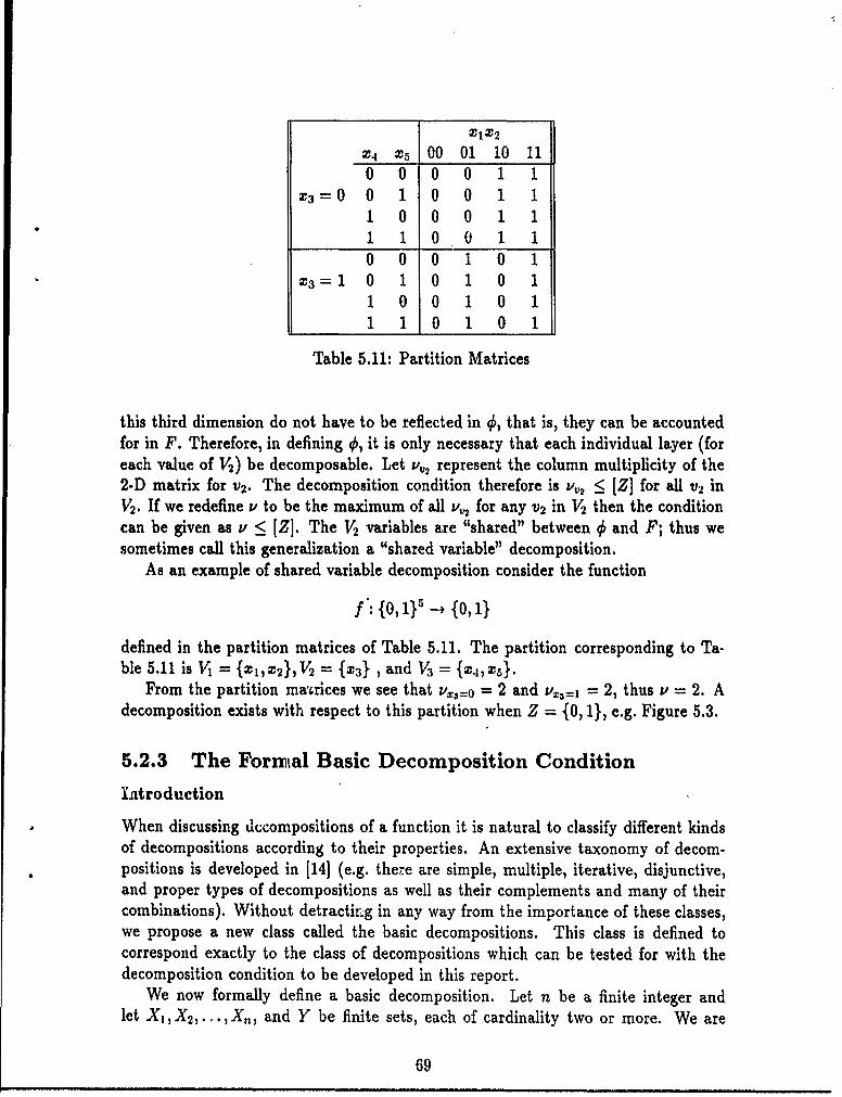
X1X 2

X4 X5 00 01 10 11

c3 =0 0 1 0 0 1 1

1 0 0 0 1 1

1 1 0 0 1 10 0 0 1 0 1

X3=1 0 1 0 1 0 11 0 0 1 0 1S1 0 1 01

Table 5.11: Partition Matrices

this third dimension do not have to be reflected in 0, that is, they can be accountedfor in F. Therefore, in defining qS, it is only necessary that each individual layer (foreach value of V2) be decomposable. Let v,, represent the column multiplicity of the2-D matrix for v2. The decomposition condition therefore is v,2 < [Z] for all v2 inV2. If we redefine v to be the maximum of all v,2 for any v2 in V2 then the conditioncan be given as v < [Z]. The V2 variables are "shared" between 4 and F; thus wesometimes call this generalization a "shared variable" decomposition.

As an example of shared variable decomposition consider the function

f: {0,1}Y -+ {0,1}

defined in the partition matrices of Table 5.11. The partition corresponding to Ta-ble 5.11 is V = {1 l,X 2 }, V 2 = {X3 }, and V3 = IX4,XS}.

From the partition ma,6rices we see that v,3=0 = 2 and V 3 = 2, thus v = 2. Adecomposition exists with respect to this partition when Z = {0, 1}, e.g. Figure 5.3.

5.2.3 The Formal Basic Decomposition ConditionIntroduction

When discussing decompositions of a function it is natural to classify different kindsof decompositions according to their properties. An extensive taxonomy of decom-positions is developed in [14] (e.g. there are simple, multiple, iterative, disjunctive,and proper types of decompositions as well as their complements and many of theircombinations). Without detractirg in any way from the importance of these classes,we propose a new class called the basic decompositions. This class is defined tocorrespond exactly to the class of decompositions which can be tested for with thedecomposition condition to be developed in this report.

We now formally define a basic decomposition. Let n be a finite integer andlet X1 , X 2,...,X,,, and Y be finite sets, each of cardinality two or more. We are

69

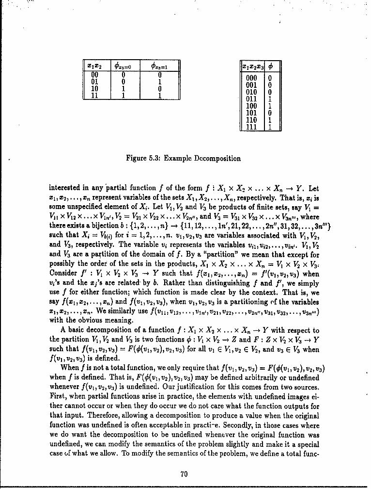
M12 0x3=O 0.3=l XlX2X3 90 00 0 000 001 0 1 001 010 1 0 010 011 1 1 011 1

100 1101 0110 1111 1

Figure 5.3: Example Decomposition

interested in any partial function f of the form f X1 x X2 x ... x X n - Y. LetXI Z2),... t, represent variables of the sets X 1,X 2,... ,X,, respectively. That is, zi issome unspecified element of Xi. Let V1, V2 and V3 be products of finite sets, say V1 =VII X V 2 X ... X V,, V2 = V21 X V22 x ... x V2,,,, and V3 = V31 X V32 X ... X V,,,, wherethere exists a bijection b: {1,2,..., n} -* {11, 12,..., ln', 21, 22,..., 2n",3, 32,..., 3n"}such that Xi = Vb() for i = 1,2,...,n. V1,v 2,V3 are variables associated with V1, V2,and V3, respectively. The variable vi represents the variables Vil, 2,... ,Vin,'. V1, V2

and V3 are a partition of the domain of f. By a "partition" we mean that except forpossibly the order of the sets in the products, X, x X 2 x ... x X,, = V1 x V2 x V3;

Consider f : V x V2 x VI -* Y such that f(XI, 2,...,X,) = f'(vI,v 2,)V3 ) whenvi's and the xj's are related by b. Rather than distinguishing f and f, we simplyuse f for either function; which function is made clear by the context. That is, wesay f(X ,Z2, ,x, ) and f(V1,v 2,v3), when vI,v 2,v 3 is a partitioning ('f the variablesX, 2,... t , ,. We similarly use f (VIi, 1 2, ... ,V1 n,,'V 21 ,) 22 ,... ,V2,, , V3 1 V 3 2, t ... , V3n)

with the obvious meaning.A basic decomposition of a function f : X1 x X 2 x ... x X, --- Y with respect to

the partition V, V2 and V3 is two functions 9 : V x V2 -4 Z and F : Z x V2 x V3 -4 Ysuch that f(VI,V 2 ,V3) = F(O(vi,v 2),v 2,v 3 ) for all vI E VI,V 2 E V2 , and v3 E V3 whenf(vI,v 2,v 3 ) is defined.

When f is not a total function, we only require that f(vI, v 2, v,) = F(9(vi, v2), v 2, v)when f is defined. That is, F(O(vl, V2 ), V2 , V3 ) may be defined arbitrarily or undefinedwhenever f(vI, v 2, v3) is undefined. Our justification for this comes from two sources.First, when partial functions arise in practice, the elements with undefined images ei-ther cannot occur or when they do occur we do not care what the function outputs forthat input. Therefore, allowing a decomposition to produce a value when the originalfunction was undefined is often acceptable in practi-e. Secondly, in those cases wherewe do want the decomposition to be undefined whentver the original function wasundefined, we can modify the semantics of the problem slightly and make it a specialcase of what we allow. To modify the semantics of the problem, we define a total func-

70

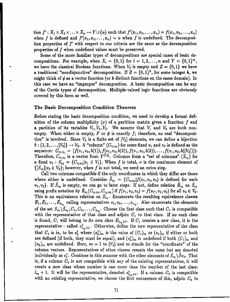
tion f: X, x X 2 x ... x X, -- YU{u} such that f'(OhO2, ... ,0n) f(0t,2,...,?O)when f is defined and f'(X1 ,X 2,. . . ,On) = u when f is undefined. The decomposi-tion properties of f with respect to our criteria are the same as the decompositionproperties of f when undefined values must be preserved.

Some of the more familiar types of decompositions are special cases of basic de-compositions. For example, when Xi = {0,1} for i = 1,2,...,n and Y = { 0 ,1}m,we have the classical Boolean functions. When V2 is empty and Z = {O, 1} we havea traditional "nondisjunctive" decomposition. If Z = {0, 1}k, for some integer k, wemight think of 0 as a vector function (or k distinct functions on the same domain). Inthis case we have an "improper" decomposition. A basic decomposition can be anyof the Curtis types of decomposition. Multiple-valued logic functions are obviouslycovered by this form as well.

The Basic Decomposition Condition Theorem

Before stating the basic decomposition condition, we need to develop a formal defi-nition of the column multiplicity (v) of a partition matrix given a function f anda partition of its variables V1, V2 , V3. We assume that V and V3 are both non-empty. When either is empty, F or q0 is exactly f; therefore, no real "decomposi-tion" is involved. Since V3 is a finite set of [V3] elements, we can define a bijectionb: {1,2,... I[V]} -+ V1. A "column" (C,,,,) for some fixed v, and v2 is defined as thesequence: C,,V. = (f(v,v 2,b(l)), f(vi,v2,b(2)),f(vI,v 2,b(3)),. . . ,f(v1,v 2,b([V]))).Therefore, C,,, 2 is a vector from Y1 31. Columns form a "set of columns" (SV2) fora fixed v2 : Sv, = {C, 2 [vl E Vl}. When f is total, v is the maximum element of{ [SvJV2 E V21; however, when f is not total, we need an extra step.

Call two columns compatible if the only coordinates in which they differ are thosewhere either is undefined. Consider §V 2 = {C, 1,2Vf(v,v 2, v3) is defined for eachv1,v3}. If S 2 is empty, we can go to later steps. If not, define relation R 2 on §V

using prefix notation by R&2 (C V2,C1V,1V 2 ) if f(vI,v 2,v3 ) = f(vI,v 2 ,v 3) for all v3 E V3.This is an equivalence relation on Se,. Enumerate the resulting equivalence classesEl, E2, .... Ei2 calling representatives el, e 2 , . . ., ev2. Also enumerate the elementsof the set S 2 \S 2, C1, C2 ,..., Ci1,. Choose the first class such that C1 is compatiblewith the representative of that class and adjoin C1 to that class. If no such classis found, C1 will belong to its own class Eiv2+1. If C creates a new class, it is therepresentative - called e!+ 1 . Otherwise, define the new representative of the classthat C, is in, to be e' where (e'),,, is the value of (CI)m or (ek)m, if either or bothare defined (if both, they must be equal), and (e'),,, is undefined if both (CI),,, and(ek)m are undefined. Here, m = 1 to [V3] and m stands for the "coordinate" of thecolumn vectors. Representatives of other classes remain the same but are denotedindividually as el. Continue in this manner with the other elements of Sv, \Sv2. Thatis, if a column C is not compatible with any of the existing representatives, it willcreate a new class whose number is one more than the number of the last class:1,2 + 1. It will be the representative, denoted e1,2 +1. If a column Ca is compatiblewith an existing representative, we choose the first occurrence of this, adjoin Ca to

71

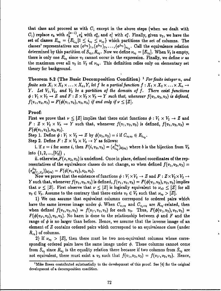
that class and proceed as with C, except in the above steps (when we dealt withCI) replace ek with ea1), 4e with ea, and- e, with e'. Finally, given v2, we have theset of classes E,2 = {Ej,2 11 < i,,: v,2 } which partitions the set of columns. Theclasses' representatives are (ejV2 ), (e j 2 )2,... , (ej

-2 )1 2 . Call the equivalence relationdetermined by this partition of S,2 , R12 . Now we define v12 = [E12]. When V2 is empty,there is only one E,2 since v2 cannot occur in the expression. Finally, we define v asthe maximum over all V2 in V2 of v,2. This definition relies only on elementary settheory for background.

Theorem 5.2 (The Basic Decomposition Condition) 1 For finite integern, andfinite sets X1 x X 2 x ... x X,, Y, let f be a partial function f : X, x X 2 x ... x X,, --

Y. Let V1, V2, and V3 be a partition of the domain of f. There exist functions4 : V1 x V2 -+ Z and F : Z x V2 x V3 -* Y such that, whenever f(vi,v 2,v 3 ) is defined,f(vI,v 2 1,v3) = F(S(v1,v2),v 2,v3 ) if and only if v < [Z].

Proof:First we prove that v < [Z implies that there exist functions q0 : V1 x V2 --+ Z andF : Z x V2 x V3 -* Y such that, whenever f(vI,v 2 ,v3 ) is defined, f(vI,v 2 ,v 3) =

Step 1. Define 4,: V x V2 --* Z by O(v,v 2) = i if C 1 12 E Ei,2Step 2. Define F : Z x V2 x V3 -- Y as follows:

i. if z = i for some i, then F(i,v2,v3) = (e i2)b(v,) where b is the bijection from V3

into {1,2,...,[V3]},ii. otherwise,F(z, v2, v3i) is undefined. Once in place, defined coordinates of the rep-

resentatives of the equivalence classes do not change, so when defined f(vi, V2,v3) -

jv2(,~~. j2 ))b(V3)= = ((jV),2V

Now we prove that the existence of functions 4 : V1 x V 2 -, Z and F : Z x V2 V3Y such that, whenever f(vI, v 2, v 3) is defined, f(v1, v 2, v 3) = F((vl, v2 ), v 2, v 3) impliesthat v < [Z]. First observe that v < [Z] is logically equivalent to v'2 < [Z] for allV2E V. Assume to the contrary that there exists v2 E V2 such that vV2 > [Z].

1) We can assume that equivalent columns correspond to ordered pairs whichhave the same inverse image under 4,. When C,,v, and C1, I V2 are R V2 -related, thenwhen defined f(v 1 ,v 2,v 3) = f(vI,,v 2 ,v3 ) for each v3. Thus, F(0(vj,v2),V2 ,v3 ) =F(0(v,,v2),v 2,v 3 ). No harm is done to the relationship between 4 and F and therange of 4 is no larger than before. Hence, we assume that the inverse image of anelement of Z contains ordered pairs which correspond to an equivalence class (underR,,,) of columns.

2) If V,2 > [Z], then there must be two non-equivalent columns whose corre-sponding ordered pairs have the same image under 4,. These columns cannot comefrom S U2 since R,2 is the equality relation there because if two columns from S 2 arenot equivalent, there must exist a v3 such that f(vI,v 2 ,v3 ) = f(vI,v 2,v3). Hence,

'Mike Breen contributed substantially to the development of this proof. See [4) for the originaldevelopment of a decomposition condition.

72

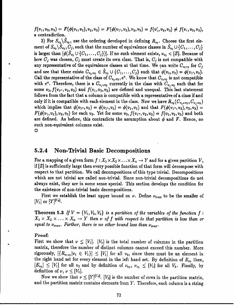
f(V1,V2,V3)= FQP(viV2),V2,V3) =F(k(ViV2),V2 ,V3) = f(cnIV 2,V3) f(VgV 2,V3),a contradiction.

3) For SV2\S 2, use the ordering developed in defining R12. Choose the first ele-ment of S, 2 \S 2, Cj, such that the number of equivalence classes in S,,2 U {Ct,... , Cj}is larger than [q(Sv2 U {C1,..., Cj})]. If no such element exists, v,2 < [Z]. Because ofhow Cj was chosen, Cj must create its own class. That is, Cj is not compatible withany representative of the equivalence classes at that time. We can write C 1,2 for Cjand see that there exists C, e S 2 U {C 1 ,...,Cj} such that q(vj,v2) = (vII,v 2).Call the representative of the class of C,, 2, ea. We know that CV 2 is not compatiblewith ea.Therefore, there is a C,11 2 currently in the class with C,,,, 2 such that forsome v3 ,f(v,,vuV3 ) and f(v 1 ,v 2,v 3) are defined and unequal. This last statementfollows from the fact that a column is compatible with a representative of a class if andonly if it is compatible with each element in the class. Now we have Rv2 (C, 111V2, CVt,,2)which implies that q(V 1,,v 2) = q(vI,v 2 ) = q(vj,v2 ) and that F(#(vI-i,V 2 ),v 2 ,v 3 ) =F((vi,v2 ),v 2,v 3) for each v3. Yet for some v3 ,f(vi,,v 2,v3 ) = f(vi,v 2,v3 ) and bothare defined. As before, this contradicts the assumption about 0 and F. Hence, nosuch non-equivalent columns exist.0

5.2.4 Non-Trivial Basic Decompositions

For a mapping of a given form f X1 x X2 ... x X, --+ Y and for a given partition V,if [Z] is sufficiently large then every possible function of that form will decompose withrespect to that partition. We call decompositions of this type trivial. Decompositionswhich are not trivial are called non-trivial. Since non-trivial decompositions do notalways exist, they are in some sense special. This section develops the condition forthe existence of non-trivial basic decompositions.

First we establish the least upper bound on v. Define Vmax to be the smaller of[V] or [y][l 1.

Theorem 5.3 If V = {V 1, V2 , V3} is a partition of the variables of the function fX1 x X 2 x ... x Xn -* Y then v of f with respect to that partition is less than orequal to vmx. Further, there is no other bound less than Umax

Proof:First we show that v < [VJ. [VIJ is the total number of columns in the partitionmatrix, therefore the number of distinct columns cannot exceed this number. Morerigorously, [{Ro1t 2Ivi E V1}] < [V] for all v2, since there must be an element inthe right hand set for every element in the left hand set. By definition of EV2 then,[E,,] < [V] for all v2 and by definition of P,,, v,, [11] for all V2 . Finally, bydefinition of v, v < [V1].

Now we show that v < [Y]1I31. [V3] is the number of rows in the partition matrix,and the partition matrix contains elements from Y. Therefore, each column is a string

73

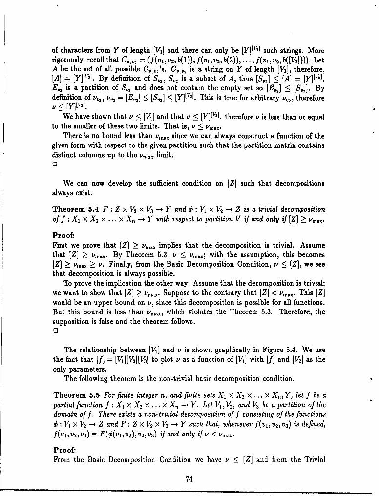
of characters from Y of length [V3] and there can only be [Y11"31 such strings. Morerigorously, recall that C,,,, = (f(vI, v 2, b(1)),f(vI, v 2, b(2)),..., f(VI, v2, b([V;]))). LetA be the set of all possible C,11,,2's. C, 1 2 is a string on Y of length [V], therefore,[A] - [Y]IN. By definition of SV2, S, is a subset of A, thus [$S21 :- [A] = [Y][IN.E,,2 is a partition of S12 and does not contain the empty set so [E,2 ] :_ [S.21. Bydefinition of vv,, vv 2 [ E2] < [S2] < [Y]V3]. This is true for arbitrary v,,, thereforeV < [Y[tV3].

We have shown that v < [V] and that v < [Y][ '3]. therefore v is less than or equalto the smaller of these two limits. That is, v < .

There is no bound less than Vmax since we can always construct a function of thegiven form with respect to the given partition such that the partition matrix containsdistinct columns up to the v,,a, limit.3

We can now develop the sufficient condition on [Z] such that decompositionsalways exist.

Theorem 5.4 F : Z x V2 x V3 -+ Y and q : V1 x V2 - Z is a trivial decompositionoff : X, x X 2 x ... x X,, --, Y with respect to partition V if and only if [Z] > vmax.

Proof:First we prove that [Z] > vnmax implies that the decomposition is trivial. Assumethat [Z] > vma.x. By Theorem 5.3, v < v,; with the assumption, this becomes(Z] _ Vz,,.x _ v,. Finally, from the Basic Decomposition Condition, v < (Z], we seethat decomposition is always possible.

To prove the implication the other way: Assume that the decomposition is trivial;we want to show that [Z] > 'aVMx. Suppose to the contrary that [Z] < Vma. This [Z]would be an upper bound on vi, since this decomposition is possible for all functions.But this bound is less than Vmax, which violates the Theorem 5.3. Therefore, thesupposition is false and the theorem follows.0

The relationship between [VI] and v is shown graphically in Figure 5.4. We usethe fact that [f] = [V1[V2][V3] to plot v as a function of [Vl with [f] and [V2] as theonly parameters.

The following theorem is the non-trivial basic decomposition condition.

Theorem 5.5 For finite integer n, and finite sets X 1 x X 2 x ... x X,,,Y, let f be apartial function f : X, x X2 x ... x X,, -- Y. Let V1, V2, and V3 be a partition of thedomain of f. There exists a non-trivial decomposition of f consisting of the functions0 : V x V2 -4 Z and F : Z x V2 x V3 -- Y such that, whenever f(vi,v 2,v 3) is defined,f(vj,v 2 ,v 3) = F((v,v 2),v 2 ,v 3) if and only if v< v

Proof:From the Basic Decomposition Condition we have v < [Z] and from the Trivial

74

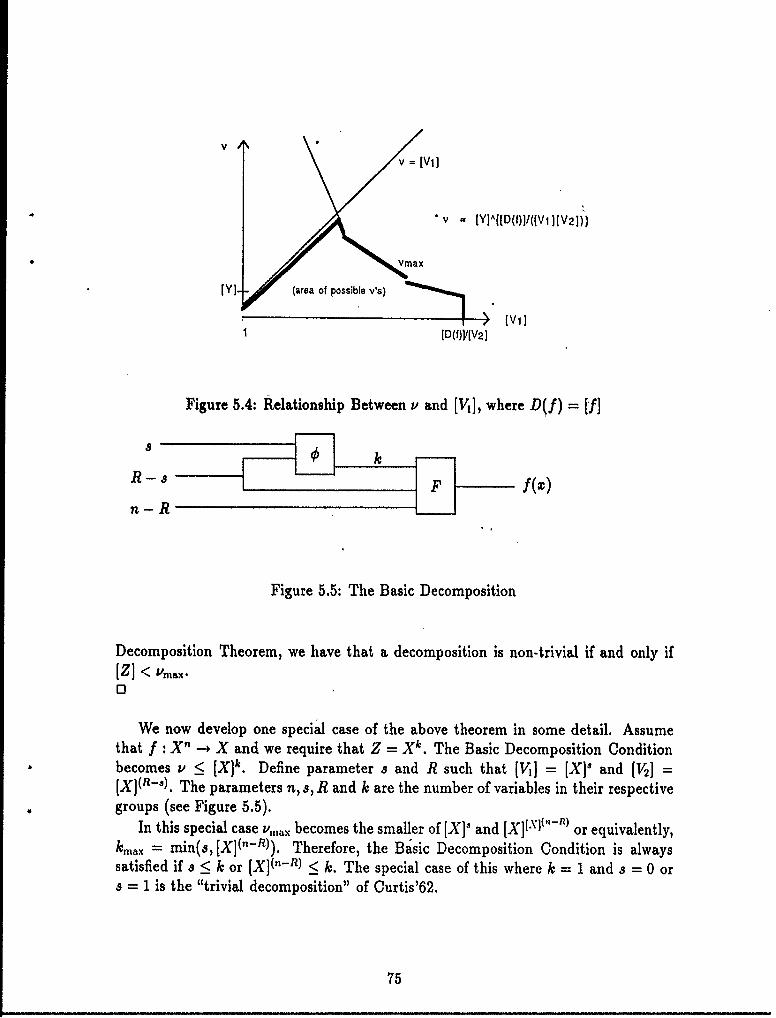
V

v= [Vi]

V = [Y]A[D(f)I/((V 1[V2])}

Vmax

[Y] (area of possible vs)

[y)~~~ ~ ~ (aeaovpsibl]v

ID(f)]/(V2]

Figure 5.4: Relationship Between v and [Vi], where D(f) = [f]

n-R

Figure 5.5: The Basic Decomposition

Decomposition Theorem, we have that a decomposition is non-trivial if and only if[Z] < Lmax.0

We now develop one special case of the above theorem in some detail. Assumethat f : Xn -4X and we require that Z = Xk. The Basic Decomposition Conditionbecomes v < [X]k. Define parameter 8 and R such that [Vi] = [X]3 and [2] =

[X](R-°). The parameters n, s, R and k are the number of variables in their respectivegroups (see Figure 5.5).

In this special case v,ax becomes the smaller of [X]' and [X][_yl(" - R ) or equivalently,kmax = min(a, [X](n-R)). Therefore, the Basic Decomposition Condition is alwayssatisfied if a < k or [X](nR) < k. The special case of this where k = 1 and S = 0 ora = 1 is the "trivial decomposition" of Curtis'62.

75

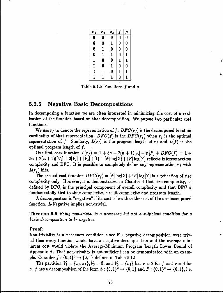
X1 X2 X3 f g0 0 0 0 0

0 0 1 0 -00 1 0 0 00 1 1 0 11 0 0 1 11 0 1 0 01 1 0 1 11 00

Table 5.12: Functions f and g

5.2.5 Negative Basic Decompositions

In decomposing a function we are often interested in minimizing the cost of a real-ization of the function based on that decomposition. We pursue two particular costfunctions.

We use rf to denote the representation of f. DFC(rf) is the decomposed functioncardinality of that representation. DFC(f) is the DFC(rj) when rf is the optimalrepresentation of f. Similarly, L(rf) is the program length of rf and L(f) is theoptimal program length of f.

Our first cost function L(rf) = 1 + 3n + 2(n + 1)[A] + n[P] + DFC(f) = 1 +5n + 2(n + 1)([V] + 2[V 2] + (V3 + '1) + [ )] log[Z] + [F] log[Y] reflects interconnectioncomplexity and DFC. It is possible to completely define any representation ry withL(rf) bits.

The second cost function DFC(rf) = [4)] log[Z] + [F] log[Y] is a reflection of sizecomplexity only. However, it is demonstrated in Chapter 4 that size complexity, asdefined by DFC, is the principal component of overall complexity and that DFC isfundamentally tied to time complexity, circuit complexity and program length.

A decomposition is "negative" if its cost is less than the cost of the un-decomposedfunction. L-Negative implies non-trivial.

Theorem 5.6 Being non-trivial is a necessary but not a sufficient condition for abasic decomposition to be negative.

Proof:Non-triviality is a necessary condition since if a negative decomposition were triv-ial then every function would have a negative decomposition and the average min-imum cost would violate the Average-Minimum Program Length Lower Bound ofAppendix A. That non-trivality is not sufficient can be demonstrated with an exam-ple. Consider f : {0, 1}' -4 {0, 1} defined in Table 5.12

The partition V = {X,X 2}, V2 = 0, and V3 = {X3} has v = 2 for f and v = 4 forg. f has a decomposition of the form 4): {0, 1} - {0, 1} and F: {0, 1}2 -+ {0, 1}, i.e.

76

Z = {0, 1}. This decomposition is non-trivial since there exists a function (namelyg) that does not have this decomposition with respect to this partition. This decom-position is also not negative. That is, L(rf) DFC(rf) = 22 + 22 = 8 which is notless than 2 3 = 8.0

Explicit statements of the various negative decomposition conditions are of interestsince they are used in decomposition algorithms. The following is called the L-Negative Basic Decomposition Condition.

Theorem 5.7 A Basic Decomposition : V x V2 --+ Z and F: Z x V2 x V, -- Y ofa function f : X 1 x X2 x ... x Xn - Y with respect to partition V is negative withrespect to L if and only if 1 + 7n + 2(n + 1)([V1] + 2[V2] + [V]) + [Vj [V2] log[Z] +[Z[V2 [V3 log[Y] < [V1][V2 [V3] log[Y].

Proof:By definition of a negative decomposition: L(rj) < [X] log[Y] + 1. The theoremfollows by substitution and simplification.0

The next theorem is the DFC-Negative Basic Decomposition Condition.

Theorem 5.8 A Basic Decomposition q! : V x V2 -+ Z and F : Z x V2 x V3 -4 Y ofa function f : X1 x X 2 x ... x Xn -* Y with respect to partition V is negative withrespect to DFC if and only if [VIllog[Z] + [Z[V3]log[yl < [V1][V] log[Y].

Proof:By definition of a negative decomposition: DFC(rf) < [X] log[Y. The theorem fol-lows by substitution and simplification.0'

The largest (Z] that satisfies the above inequalities is the largest [Z] that willyield a negative decomposition in the applicable situation. Since [Z] must be greaterthan or equal to the column multiplicity v, the above inequalities give the maximumv that will result in a negative decomposition. Therefore, when we are exclusivelyinterested in negative decompositions, we are only interested in v's which satisfy theabove inequalities. That is, in the DFC case, [VI] log v + v[V.j] log[Y] < [V1][V11 log[Y].If vmax is the largest integer that satisfies the negative decomposition condition thenwe are only interested in v's which are less than or equal to Vmax. Therefore, when weare counting columns in a partition matrix, we can stop counting as soon as v reaches

-,,ax. With respect to our special case of the previous section (i.e. f : X" --+ X, Z =Xk, XV = X 8 ,2 = X(R-.), and V3 = X("-")) the DFC-Negative decompositioncondition becomes k[X]' + [X](k+--R) < [X]. That is, from the theorem above:

[V19log[ZJ + [Z][V log[Y] < [ V][V]log[Y],

77

[X] ° log([x]k) + [x]k[x](n - R) log[X] < [X]O[X](n-") log[X],

k[X]5 log[X] + [X](k+n- R) log[X] < [X](n-R+s) log[X],

k[Xj + [X](k+n-R) < [X](n-R+).

With the further specialization that there be no shared variables (i.e. R = 8), thecondition becomes k[X]R + [X](k+n- R) < [X](") or k[X](R-n) + [X](k-R) < 1.

If we define kmax as the largest integer satisfying the applicable condition thenwe know that k must be less than or equal to kmax for negative decompositions. Itfollows then that the maximum v of interest is inax = [X]kmax.

The important point is that, given n and V, we can directly determine the maxi-mum v for a negative decomposition. This test can be useful since we may want todiscontinue counting columns in evaluating column multiplicity after we are assuredthat no negative decomposition is possible.

We have one final result concerning basic decompositions. Let N be the numberof ways that a set X can be partitioned into three sets V1, V2, V3 .2 The number ofcombinations of i elements from the set X, where X has n elements, is n!/(n - i)! =C(n, i). This takes care of the first set V1. Now select j elements from n - i elements:(n - i)/(n-i -j)! = C(n -i,j) where j elements go into V2 and (n-i-j) elementsgo into V3 . Thus the number of combinations for one partition is C(n, i)C(n - ij).

For each i there are different combinations of n - i elements, so for all partitions,the number of different combinations is:

n n-i

N E E (ni)C(n-i,j)i=U j=O

nn-i

=jC(n, i) E C(n - i,j)i=0 j=0

i n-i n

= C(n,i)1' F C(n - ij)lO'--)l(i) = Z C(n,i)l(1 + 1)(i)(i=0 j=O i=0

Recalling the Binomial Theorem [41, p.27]:

n

(a + b)" = E C(n, i)a (')b',i=U

N = _ C(n,i)li2(n - ) = (1 + 2)n = 3n.i=0

The number of nontrivial partitions (N') can be derived by the same method.We must make sure that V has no less than two elements and no more than n - 2elements, so i will go from two to n - 2. Also V2 can have zero elements, but no more

2This result was developed by Tina Normand.

78

than n - i - 2 elements, (to make sure V3 has at least 2 elements), so j will.go fromzero to n - i - 2. The result is:

n-2 m-i-2N'=r, E C(n,i)C(n- i,j)i=2 j=O

n-2 n-i-2

= Z C(n,i) E C(n -ij)1(n-i)i(n-i-)i=2 j=O

n-2

= E C(n,i)(2'- C(n - i,n - i- 1) - C(n - i,n - i))i=2

n-2

-E C(n,i)(2' - (n-) - 1)i=2

n-2 n-2 n-2

- LG(n,i)2'-(n + 1) E C(n,i) + E C(n,i).i=2 i=2 i=2

This can be further reduced since E,'=oiC(n,i) = n2(n - 1) [65, p7l].

5.3 The Ada Function Decomposition Programs

The PT 1 function decomposition algorithm takes a binary partial function of theform f : {0, 1}n --- {, 1} and attempts to decompose the function into components0 and F such that f(x,y,z) = F(4(m,y),y,z) where x, y, and z are vectors. We areespecially interested in decompositions where the size of the decomposition (i.e. thesize of F plus the size of 0) is less than the size of the original function. The algorithmaccomplishes this decomposition by searching through all possible partitions of inputvariables and testing to see if the function decomposes for that partition. The test fordecomposition and other theoretical aspects of function decomposition are developedin the preceding section. If the function does not decompose with respect to a givenpartition then another partition is tried. If the function does decompose then anattempt is made to decompose each of the component functions. As the algorithmsearches through possible decompositions, any decomposition which has lower costthan any previous decomposition is recorded. When the search is completed, we havethe lowest cost decomposition (lowest cost of those considered) of the input function.

Several versions of this function decomposition algorithm were implemented inAda during the PT 1 project. This section describes these programs. A User's Guidefor the AFD program is in Appendix B. The PT 1 function decomposition softwarewas written in Ada on the VMS System running on a Vax 11/780. This Vax is partof the Fire Control Simulation (FICSIM) Facility of WL/AART located in Building22 at Wright Patterson AFB, Ohio.

79

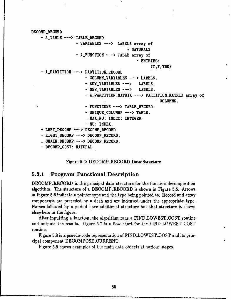
DECONPRECORD- A-TABLE --- > TABLE-RECORD

- VARIABLES --- > LABELS array of

- NATURALS- A-FUNCTION ---> TABLE array of

- ENTRIES:

(T,F,TBD)- A-PARTITION --- > PARTITION-RECORD

- COLUMN-VARIABLES ---> LABELS.

- ROW-VARIABLES ---> LABELS.- NEW-VARIABLES ---> LABELS.

- APARTITIONMATRIX --- > PARTITION-MATRIX array of- COLUMNS.

- FUNCTIONS ---> TABLE-RECORD.

- UNIQUE-COLUMNS ---> TABLE.- MAXNU: INDEX: INTEGER- NU: INDEX.

- LEFTDECOMP ---> DECOMPRECORD.

- RIGHTDECOMP ---> DECOMPRECORD.- CHAINDECOMP ---> DECOMPRECORD.

- DECONPCOST: NATURAL

Figure 5.6: DECOMP-RECORD Data: Structure

5.3.1 Program Functional Description

DECOMP-RECORD is the principal data structure for the function decompositionalgorithm. The structure of a DECOMPRECORD is shown in Figure 5.6. Arrowsin Figure 5.6 indicate a pointer type and the type being pointed to. Record and arraycomponents are preceded by a dash and are indented under the appropriate type.Names followed by a period have additional structure but that structure is shownelsewhere in the figure.

After inputting a function, the-algorithm runs a FIND.LOWEST-COST routineand outputs the results. Figure 5.7 is a flow chart for the FINDJOWESTCOSTroutine.

Figure 5.8 is a psuedo-code representation of FIND-LOWESTCOST and its prin-cipal component DECOMPOSE-CURRENT.

Figure 5.9 shows examples of the main data objects at various stages.

80

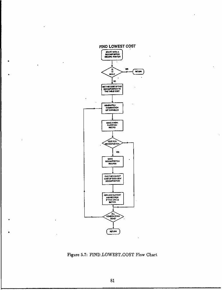
FIND LOWEST COSTSTART MM~ A

is yIT

'D

IETAU.EOST

Of VAAALES

PARTITIN

TEST FR

MWcE

FWD THE LOWEST

COTOF EAH NE

RUMCE OST" RM.

IFhIS ONE IS

AL.

Figure 5.7: FIND-.LOWESL-COST Flow Chart

81

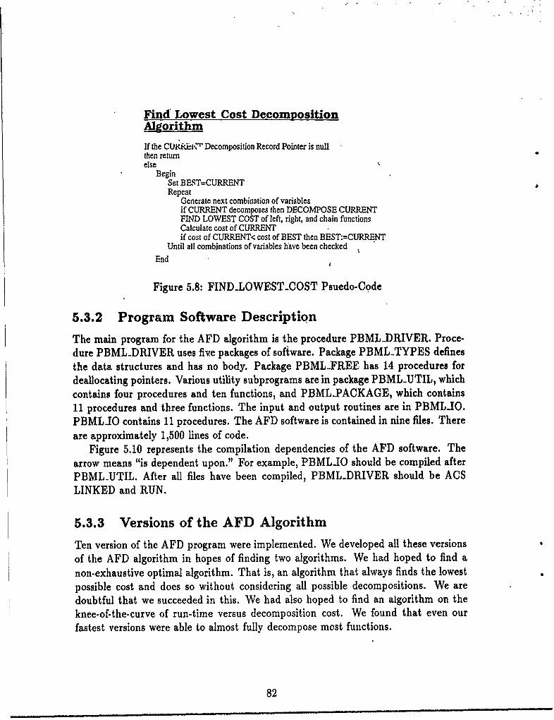
Find Lowest Cost DecompositionAlgorithm

If the CUR-€t'Z Decomposition Record Pointer is nullthen returnelse

BeginSet BEST=CURRENTRepeat

Generate next combination of variablesif CURRENT decomposes then DECOMPOSE CURRENTFIND LOWEST COST of left, right, and chain functionsCalculate cost of CURRENTif cost of CURRENT< cost of BEST then BEST:=CURRENT

Until all combinations of variables have been checked

End

Figure 5.8: FINDLOWEST-COST Psuedo-Code

5.3.2 Program Software Description

The main program for the AFD algorithm is the procedure PBMLDRIVER. Proce-dure PBMLDRIVER uses five packages of software. Package PBMLTYPES definesthe data structures and has no body. Package PBMLFREE has 14 procedures fordeallocating pointers. Various utility subprograms are in package PBMLUTIL, whichcontains four procedures and ten functions, and PBMLPACKAGE, which contains11 procedures and three functions. The input and output routines are in PBML-IO.PBMLJO contains 11 procedures. The AFD software is contained in nine files. Thereare approximately 1,500 lines of code.

Figure 5.10 represents the compilation dependencies of the AFD software. Thearrow means "is dependent upon." For example, PBML_IO should be compiled afterPBMLUTIL. After all files have been compiled, PBML.DRIVER should be ACSLINKED and RUN.

5.3.3 Versions of the AFD Algorithm

Ten version of the AFD program were implemented. We developed all these versionsof the AFD algorithm in hopes of finding two algorithms. We had hoped to find anon-exhaustive optimal algorithm. That is, an algorithm that always finds the lowestpossible cost and does so without considering all possible decompositions. We aredoubtful that we succeeded in this. We had also hoped to find an algorithm on theknee-of-the-curve of run-time versus decomposition cost. We found that even ourfastest versions were able to almost fully decompose most functions.

82

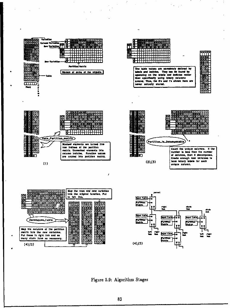
eperttabesIn g sim e thelbl stIdctrse

0

Pa1edel1,t11 tur ne 'mte Pstte .s.....e peat1! 7 row In~s "M the "INGartltlonw

metIBMT "snug ascae oftements ]MoeadIic Intoy aun the funi u b oun.y hcoum Tablee Functiot; asne telbsanme Md e~ rathen th 0umear cohie intololl usittio maaj e column@,te tdoepss

"hMIe binryl stabels 1or eacC 1 atA)unqeceun

3 IT I oi

aa

rowInlo f hepaFiour 5.9:t Alorth Stquaclmnges h

motll.Un ake eemns nt nmbrIsbe te te83me

Organization of PBML Code

procedure PBML_DRIVER

Vpackage PBM.PACKAGE

Vpackage PBMLIO

Vpackage PBMLUTIL

IV

package PBMLFRBE

Vpackage PBML_TYPES

Figure 5.10: Compilation Dependencies

Search Constraints Common to All Versions

An exhaustive search approach to function decomposition becomes intractable forfunctions on more than two or three vari.bles. Therefore, it is necessary to limitthe search. There are some search limits that all the versions have in common. Fora given partition of variables, the basic approach of each version is to compute thecolumn multiplicity v of the function with respect to that partition. The value ofv is then compared to a threshold that is version dependent. If the threshold isexceeded then this decomposition is dropped from further consideration. The ideais that we only want to pursue decompositions that are reducing cost. It is in howmuch of a reduction we want or how we measure cost that the versions differ. For ourhighest threshold (i.e. most exhaustive search) we know of no functions where a moreexhaustive search would produce a lower overall cost decomposition. However, forour other thresholds we know that some desirable decompositions are being dropped.Using this threshold significantly reduces the search space; since otherwise everypartition yields a decomposition whose children must be decomposed before we knowthat it will not result in an lower overall cost.

When the threshold is not exceeded and the decomposition is pursued, the firststep is to form the children of the decomposition, F and 4. All the versions formF and 4' by using the binary equivalent of an enumeration of the columns generatedin counting up the column multiplicity. This simple approach to defining F and 4'substantially reduces the overall search space. There are typically many different F'sand O's for a given decomposition. At least in some cases, how F and 4' are definedaffects the decomposability of F and 4' and, consequently, the eventual cost of theoverall decomposition. Therefore, to be exhaustive, we must assess the decompos-ability of all the different possible values for F and 4, before arriving at a specific F

84

and q. None of the AFD versions did this.

Search Constraint Differences Between Versions

There are two classes of variable partitions used by the AFD algorithms. Version 1and all the 2 versions (i.e. 2, 2a, 2b, 2ab) partition the variables into two disjoint sets.One set is input into F and the other into q. Version 3 and all the 4 (i.e. 4, 4a, 4b,4ab) versions partition the variables into three disjoint sets. One set is input into Fonly, the second set is input into q only, and the third set is input to both F and 0.We call this latter class of partitions the "shared variable" class while the first classis cailed "no-shared variables." When only no-shared variable partitions are used ina search it is possible for the specific values assigned to F and 0 to affect the costof the overall decomposition. We know of no cases where the method of assigningvalues to F and 0 affects the overall decomposition when shared variable partitionsare used in the search. It is possible that one has an alternative between searchingthrough values for F and 0 and searching with shared variable partitions; with eitherapproach resulting in optimal decompositions.

The "a" versions (i.e. versions 2a, 2ab, 4a and 4ab) differ from the other versionsin that they are "greedy." The "" versions search through partitions in order ofincreasing numbers of variables input into 0. When a cost saving decomposition isfound for some number of input variables into 0 then partitions with a larger numberof variables input into 0 are not considered. That is, once a decomposition is foundfor some number of variables into 0 we pursue that decomposition but do not backupto consider larger numbers of inputs into 4. The idea here is that we want to breakthe original function into pieces that are as small as possible. Therefore, when wehave succeeded in breaking out a small piece, we do not worry about trying to breakout a larger piece. The "a" versions run substantially faster than the other versionsand perform only slightly worse in terms of the cost of the decompositions produced.

As discussed previously, the AFD algorithms compare the cost of a candidatedecomposition to a threshold. There are two methods for computing the cost of acandidate decomposition. The "b" versions (i.e. version 2b, 2ab, 4b, 4ab) computecost based on the cardinality of the components (DPFC). The other versions computecost based on the number of variables input into each component of the decomposition(DFC). That is,

DPFC= [pi]PiEll

andDFC = Z 2".

pIEP

When the components are total functions the two costs are the same. However,when a component is a partial function, which can occur even when the input is atotal function, DPFC is less than DFC. Since candidate decompositions are pursuedwhenever the cost is less than the threshold, "b" versions will in general conduct alarger search.

85

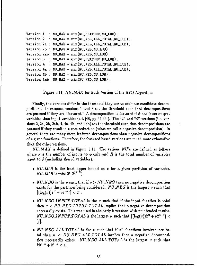
Version 1 : NUMAX = min(NUFEATURENULUB).

Version 2 : NUMAX = min(NUNEGALLTOTAL,NULUB).

Version 2a : NUMAX = min(NU_NEGALL_TOTAL,NULUB).

Version 2b : NUMAX = min(NUNEG,NULUB).

Version 2ab: NUMAX = min(NUNEG,NULUB).Version 3 : NUMAX = min(NU_FEATURE,NULUB).

Version 4 : NUMAX = min(NU_NEGALLTOTAL,NULUB).

Version 4a : NUMAX = min(NU_NEGALLTOTAL,NU_LUB).

Version 4b : NUMAX = min(NUNEG,NULUB).

Version 4ab: NUMAX = min(NUNEG,NULUB).

Figure 5.11: NUMAX for Each Version of the AFD Algorithm

Finally, the versions differ in the threshold they use to evaluate candidate decom-positions. In essence, versions 1 and 3 set the threshold such that decompositionsare pursued if they are "featured." A decomposition is featured if 4 has fewer outputvariables than input variables (c.f. [48, pp.64-66]). The "2" and "4" versions (i.e. ver-sions 2, 2a, 2b, 2ab, 4, 4a, 4b, and 4ab) set the threshold such that decompositions arepursued if they result in a cost reduction (what we call a negative decomposition). Ingeneral there are many more featured decompositions than negative decompositionsof a given functions. Therefore, the featured based versions are much more exhaustivethan the other versions.

NUMAX is defined in Figure 5.11. The various NU's are defined as followswhere a is the number of inputs to 0 only and R is the total number of variablesinput to qS (including shared variables).

* NULUB is the least upper bound on v for a given partition of variables.NU.LUB is min(2-,22"- ).

* NU.NEG is the v such that if v > NUNEG then no negative decompositionexists for the partition being considered. NUNEG is the largest v such that[(log(v))21? + v2"-'1 < 2".

* NU.NEGINPUTTOTAL is the v such that if the input function is totalthen v < NUNEGINPUTTOTAL implies that a negative decompositionnecessarily exists. This was used in the early b versions with unintended results.NUNEGINPUTTOTAL is the largest v such that [(log(v))2 R + v2" 8] <[f].

* NUNEGALL-TOTAL is the v such that if all functions involved are to-tal then v < NU.NEGALLTOTAL implies that a negative decomposi-tion necessarily exists. NU.NEGALLTOTAL is the largest v such thatk2r-' + 2 k-s < 1.

86

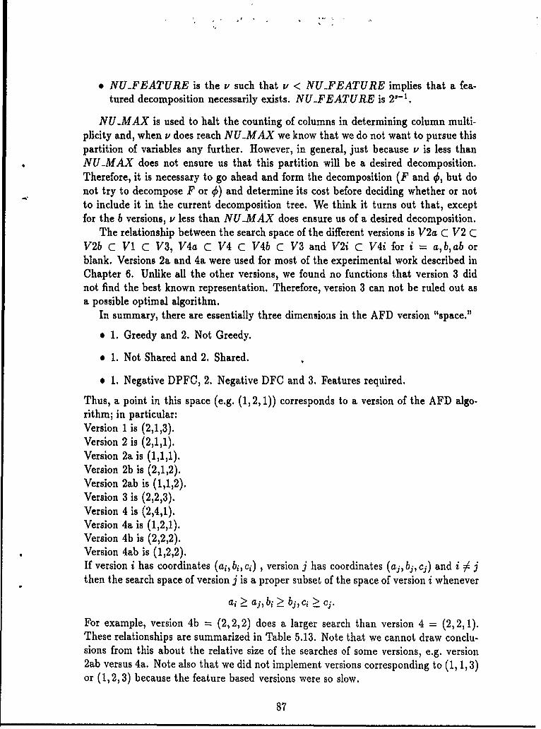
* NUFEATURE is the v such that v < NUFEATURE implies that a fea-tured decomposition necessarily exists. NU-FEATURE is 2 - 1.

NUMAX is used to halt the counting of columns in determining column multi-plicity and, when v does reach NUMAX we know that we do not want to pursue thispartition of variables any further. However, in general, just because v is less thanNU-MAX does not ensure us that this partition will be a desired decomposition.Therefore, it is necessary to go ahead and form the decomposition (F and 0, but donot try to decompose F or 0) and determine its cost before deciding whether or notto include it in the current decomposition tree. We think it turns out that, exceptfor the b versions, v less than NUMAX does ensure us of a desired decomposition.

The relationship between the search space of the different versions is V2a C V2 CV2b C V1 C V3, V4a C V4 C V4b C V3 and V2i C V4i for i = a,b, ab orblank. Versions 2a and 4a were used for most of the experimental work described inChapter 6. Unlike all the other versions, we found no functions that version 3 didnot find the best known representation. Therefore, version 3 can not be ruled out asa possible optimal algorithm.

In summary, there are essentially three dimensioas in the AFD version "space."

* 1. Greedy and 2. Not Greedy.

. 1. Not Shared and 2. Shared.

* 1. Negative DPFC, 2. Negative DFC and 3. Features required.

Thus, a point in this space (e.g. (1, 2,1)) corresponds to a version of the AFD algo-rithm; in particular:Version 1 is (2,1,3).Version 2 is (2,1,1).Version 2a is (1,1,1).Version 2b is (2,1,2).Version 2ab is (1,1,2).Version 3 is (2,2,3).Version 4 is (2,4,1).Version 4a is (1,2,1).Version 4b is (2,2,2).Version 4ab is (1,2,2).If version i has coordinates (ai, bi, ci), version j has coordinates (aj, bj, cj) and i Jthen the search space of version j is a proper subset of the space of version i whenever

ai >_ aj, bi > bj, ci >_ c1 .

For example, version 4b = (2,2,2) does a larger search than version 4 = (2, 2,1).These relationships are summarized in Table 5.13. Note that we cannot draw conclu-sions from this about the relative size of the searches of some versions, e.g. version2ab versus 4a. Note also that we did not implement versions corresponding to (1, 1, 3)or (1, 2, 3) because the feature based versions were so slow.

87

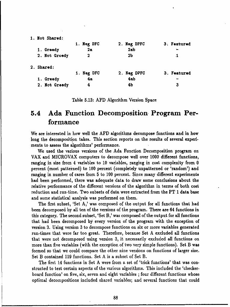
1. Not Shared:i. Neg DFC 2. Neg DPFC 3; Featured

1. Greedy 2a 2ab2. Not Groedy 2 2b I

2. Shared:i. Neg DFC 2. Neg DPFC 3. Featured

1. Greedy 4a 4ab -

2. Not Greedy 4 4b 3

Table 5.13: AFD Algorithm Version Space

5.4 Ada Function Decomposition Program Per-formance

We are interested in how well the AFD algorithms decompose functions and in howlong the decomposition takes. This section reports on the results of several experi-ments to assess the algorithms' performance.

We used the various versions of the Ada Function Decomposition program onVAX and MICROVAX computers to decompose well over 1000 different functions,ranging in size from 4 variables to 10 variables, ranging in cost complexity from 0percent (most patterned) to 100 percent (completely unpatterned or 'random') andranging in number of cares from 5 to 100 percent. Since many different experimentshad been performed, there was adequate data to draw some conclusions about therelative performance of the different versions of the algorithm in terms of both costreduction and run-time. Two subsets of data were extracted from the PT 1 data baseand some statistical analysis was performed on them.

The first subset, 'Set A,' was composed of the output for all functions that hadbeen decomposed by all ten of the versions of the program. There are 64 functions inthis category. The second subset, 'Set B,' was composed of the output for all functionsthat had been decomposed by every version of the program with the exception ofversion 3. Using version 3 to decompose functions on six or more variables generatedrun-times that were far too great. Therefore, because Set A excluded all functionsthat were not decomposed using version 3, it necessarily excluded all functions onmore than five variables (with the exception of two very simple functions). Set B wasformed so that we could compare the other nine versions on functions of larger size.Set B contained 119 functions. Set A is a subset of Set B.

The first 14 functions in Set A were from a set of 'trick functions' that was con-structed to test certain aspects of the various algorithms. This included the 'checker-board function' on five, six, seven and eight variables ; four different functions whoseoptimal decompositions included shared variables; and several functions that could

88

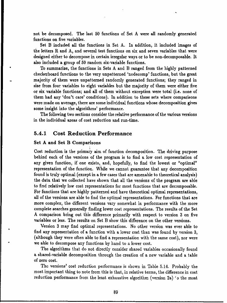
not be decomposed. The last 50 functions of Set A were all randomly generatedfunctions on five variables.

Set B included all the functions in Set A. In addition, it included images ofthe letters R and A, and several test functions on six and seven variables that weredesigned either to decompose in certain irregular ways or to be non-decomposable. Italso included a group of 50 random six-variable functions.

To summarize, the functions in Sets A and B ranged from the highly patternedcheckerboard functions to the very unpatterned 'nodecomp' functions, but the greatmajority of them were unpatterned randomly generated functions; they ranged insize from four variables to eight variables but the majority of them were either fiveor six variable functions; and all of them without exception were total (i.e. none ofthem had any 'don't care' conditions). In addition to these sets where comparisonswere made on average, there are some individual functions whose decomposition givessome insight into the algorithms' performance.

The following two sections consider the relative performance of the various versionsin the individual areas of cost reduction and run-time.

5.4.1 Cost Reduction Performance

Set A and Set B Comparisons

Cost reduction is the primary aim of function decomposition. The driving purposebehind each of the versions of the program is to find a low cost representation ofany given function, if one exists, and, hopefully, to find the lowest or "optimal"representation of the function. While we cannot guarantee that any decompositionfound is truly optimal (except in a few cases that are amenable to theoretical analysis)the data that we collected have shown that all the versions of the program are ableto find relatively low cost representations for most functions that are decomposable.For functions that are highly patterned and have theoretical optimal representations,all of the versions are able to find the optimal representations. For functions that aremore complex, the different versions vary somewhat in performance with the morecomplete searches generally finding lower cost representations. The results of the SetA comparison bring out this difference primarily with respect to version 3 on fivevariables or less. The results on Set B show this difference on the other versions.

Version 3 may find optimal representations. No other version was ever able tofind any representation of a function with a lower cost than was found by version 3,(although they were often able to find a representation with the same cost), nor werewe able to decompose any functions by hand to a lower cost.

The algorithms that do not directly consider shared variables occasionally founda shared-variable decomposition through the creation of a new variable and a tableof zero cost.

The versions' cost reduction performance is shown in Table 5.14. Probably themost important thing to note from this is that, in relative terms, the difference in costreduction performance from the least exhaustive algorithm (version 2a) 'D the most

89

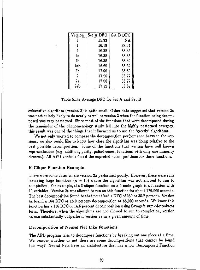
Version Set A DFC Set B DFC3 15.93 NA1 16.19 38.344 16.38 38.35

4a 16.38 38.354b 16.38 38.394ab 16.69 38.522b 17.00 38.692 17.06 38.72

2a 17.06 38.722ab 17.12 38.69

Table 5.14: Average DFC for Set A and Set B

exhaustive algorithm (version 3) is quite small. Other data suggested that version 2awas particularly likely to do nearly as well as version 3 when the function being decom-posed was very patterned. Since most of the functions that were decomposed duringthe remainder of the phenomenology study fell into the highly patterned category,this result was one of the things that influenced us to use the 'greedy' algorithms.

We not only wanted to compare the decomposition performance between the ver-sions, we also would like to know how close the algorithm was doing relative to thebest possible decomposition. Some of the functions that we ran have well knownrepresentations (e.g. addition, parity, palindromes, functions with only one minorityelement). All AFD versions found the expected decompositions for these functions.

K-Clique Function Example

There were some cases where version 2a performed poorly. However, these were runsinvolving large functions (n = 10) where the algorithm was not allowed to run tocompletion. For example, the 3-clique function on a 5-node graph is a function with10 variables. Version 2a was allowed to run on this function for about 170,000 seconds.The best decomposition found to that point had a DFC of 360 or 35.2 percent. Version4a found a 164 DFC or 16.0 percent decomposition at 65,000 seconds. We know thisfunction has a 116 DFC or 14.5 percent decomposition using Savage's sum-of-productsform. Therefore, when the algorithms are not allowed to run to completion, version4a can substantially out'perform version 2a in a given amount of time.

Decomposition of Neural Net Like Functions

The AFD program tries to decompose functions by breaking out one piece at a time.We wonder whether or not there are some decompositions that cannot be foundthis way? Neural Nets have an architecture that has a low Decomposed Function

90

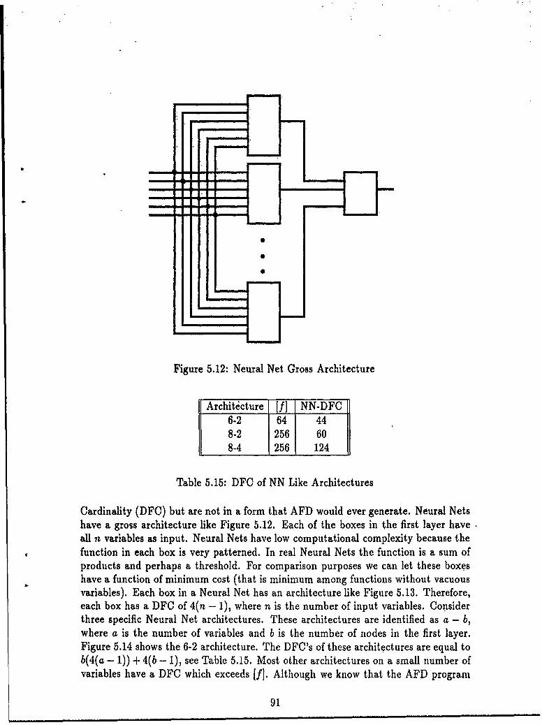
Figure 5.12: Neural Net Gross Architecture

Architecture [f] NN-DFC6-2 64 448-2 256 608-4 256 124

Table 5.15: DFO of NN Like Architectures

Cardinality (DFC) but are not in a form that AFD would ever generate. Neural Netshave a gross architecture like Figure 5.12. Each of the boxes in the first layer haveall n variables as input. Neural Nets have low computational complexity because thefunction in each box is very patterned. In real Neural Nets the function is a sum ofproducts and perhaps a threshold. For comparison purposes we can let these boxeshave a function of minimum cost (that is minimum among functions without vacuousvariables). Each box in a Neural Net has an architecture like Figure 5.13. Therefore,each box has a DFC of 4(n - 1), where n is the number of input variables. Considerthree specific Neural Net architectures. These architectures are identified as a - biwhere a is the number of variables and b is the number of nodes in the first layer.Figure 5.14 shows the 6-2 architecture. The DFC's of these architectures are equal tob(4(a - 1)) + 4(b - 1), see Table 5.15. Most other architectures on a small number ofvariables have a DFC which exceeds [f]. Although we know that the AFD program

91

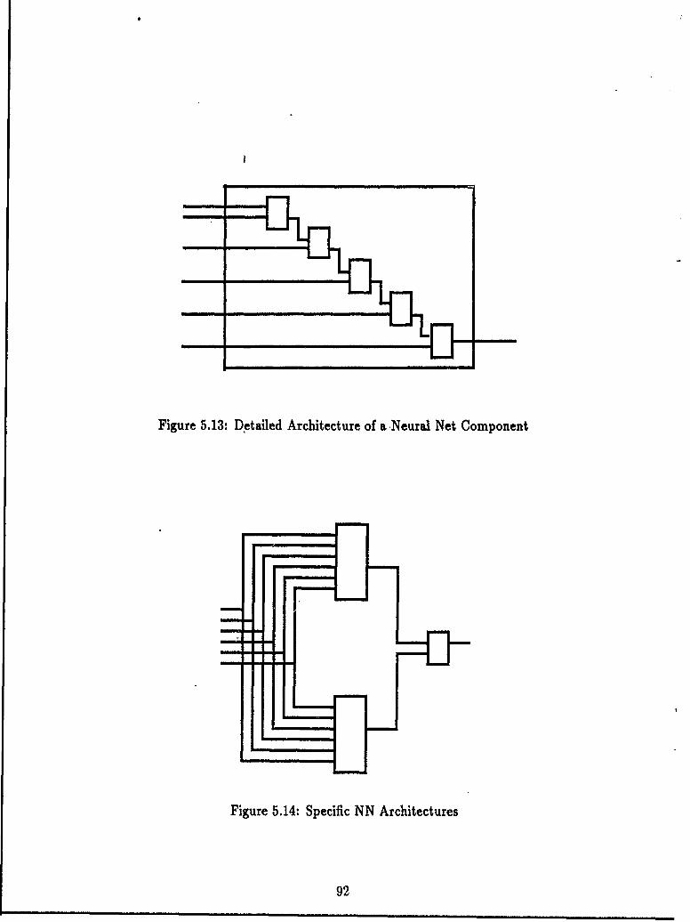
Figure 5.13: Detailed Architecture of a, Neural Net Component

----- j

Figure 5.14: Specific NN Architectures

92

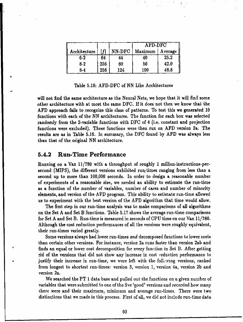
C

AFD-DFCArchitecture [f] NN-DFC Maximum Average

6-2 64 44 40 25.28-2 256 60 56 42.08-4 256 124 100 48.8

Table 5.16: AFD-DFC of NN Like Architectures

will not find the same architecture as the Neural Nets, we hope that it will findl someother architecture with at most the same DFC. If it does not then we know that theAFD approach fails to recognize this class of patterns. To test this we generated 10functions with each of the NN architectures. The function for each box was selectedrandomly from the 2-variable functions with DFC of 4 (i.e. constant and projectionfunctions were excluded). These functions were then run on AFD version 2a. Theresults are as in Table 5.16. In summary, the DFC found by AFD was always lessthan that of the original NN architecture.

5.4.2 Run-Time Performance

Running on a Vax 11/780 with a throughput of roughly 1 million-instructions-per-second (MIPS), the different versions exhibited run-times ranging from less than asecond up to more than 100,000 seconds. In order to design a reasonable numberof experiments of a reasonable size, we needed an ability to estimate the run-timeas a function of the number of variables, number of cares and number of minorityelements, and version of the AFD program. This ability to estimate run-time allowedus to experiment with the best version of the AFD algorithm that time would allow.

The first step in our run-time analysis was to make comparisons of all algorithmson the Set A and Set B functions. Table 5.17 shows the average run-time comparisonsfor Set A and Set B. Run-time is measured in seconds of CPU time on our Vax 11/780.Although the cost reduction performances of all the versions were roughly equivalent,their run-times varied greatly.

Some versions always had lower run-times and decomposed functions to lower coststhan certain other versions. For instance, version 2a runs faster than version 2ab andfinds an equal or lower cost decomposition for every function in Set B. After gettingrid of the versions that did not show any increase in cost r.eduction performance tojustify their increase in run-time, we were left with the follvwing versions, rankedfrom longest to shortest run-times: version 3, version 1, version 4a, version 2b andversion 2a.

We searched the PT 1 data base and pulled out the functions on a given number ofvariables that were submitted to one of the five 'good' versions and recorded how manythere were and their maximum, minimum and average run-times. There were twodistinctions that we made in this process. First of all, we did not include run-time data

93

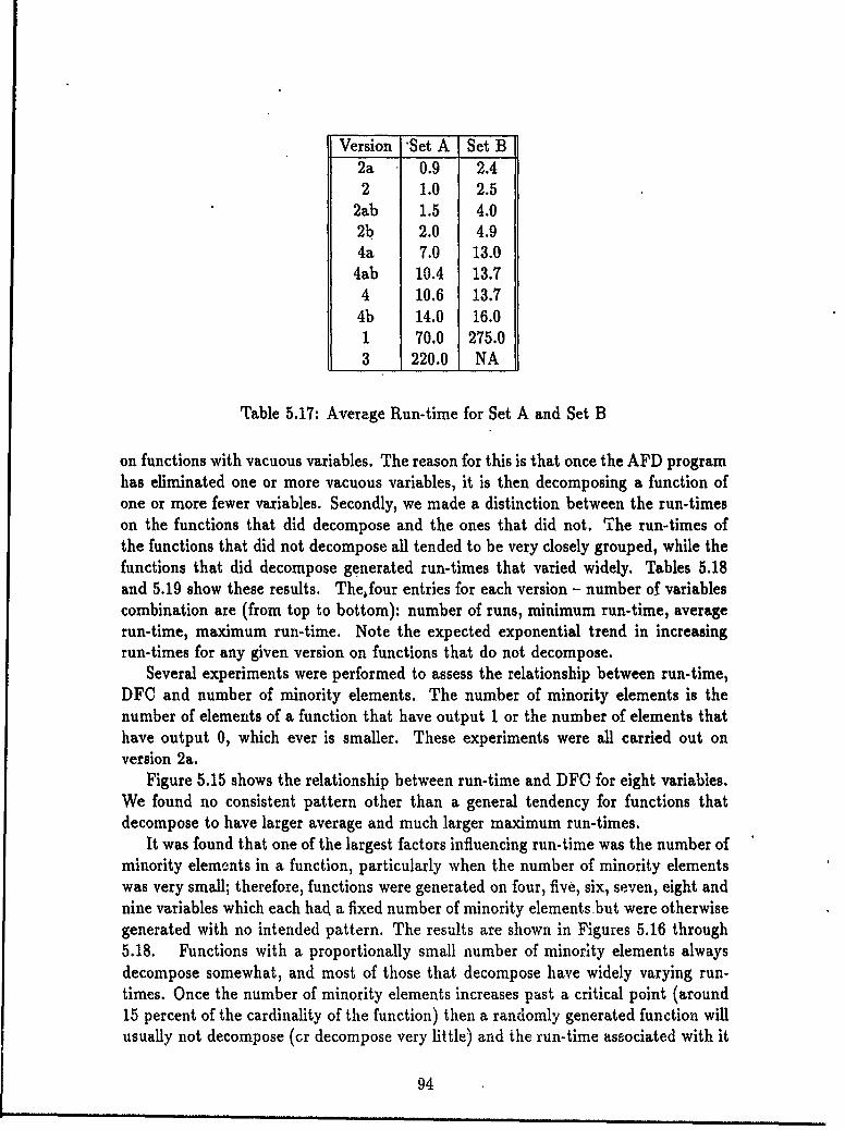
Version "Set A Set B2a 0.9 2.42 1.0 2.5

2ab 1.5 4.02b 2.0 4.94a 7.0 13.0

4ab 10.4 13.74 10.6 13.7

4b 14.0 16.01 70.0 275.03 220.0 NA

Table 5.17: Average Run-time for Set A and Set B

on functions with vacuous variables. The reason for this is that once the AFD programhas eliminated one or more vacuous variables, it is then decomposing a function ofone or more fewer variables. Secondly, we made a distinction between the run-timeson the functions that did decompose and the ones that did not. The run-times ofthe functions that did not decompose all tended to be very closely grouped, while thefunctions that did decompose generated run-times that varied widely. Tables 5.18and 5.19 show these results. Thefour entries for each version - number of variablescombination are (from top to bottom): number of runs, minimum run-time, averagerun-time, maximum run-time. Note the expected exponential trend in increasingrun-times for any given version on functions that do not decompose.

Several experiments were performed to assess the relationship between run-time,DFC and number of minority elements. The number of minority elements is thenumber of elements of a function that have output 1 or the number of elements thathave output 0, which ever is smaller. These experiments were all carried out onversion 2a.

Figure 5.15 shows the relationship between run-time and DFC for eight variables.We found no consistent pattern other than a general tendency for functions thatdecompose to have larger average and much larger maximum run-times.

It was found that one of the largest factors influencing run-time was the number ofminority elements in a function, particularly when the number of minority elementswas very small; therefore, functions were generated on four, five, six, seven, eight andnine variables which each had a fixed number of minority elements but were otherwisegenerated with no intended pattern. The results are shown in Figures 5.16 through5.18. Functions with a proportionally small number of minority elements alwaysdecompose somewhat, and most of those that decompose have widely varying run-times. Once the number of minority elements increases past a critical point (around15 percent of the cardinality of the function) then a randomly generated function willusually not decompose (or decompose very little) and the run-time associated with it

94

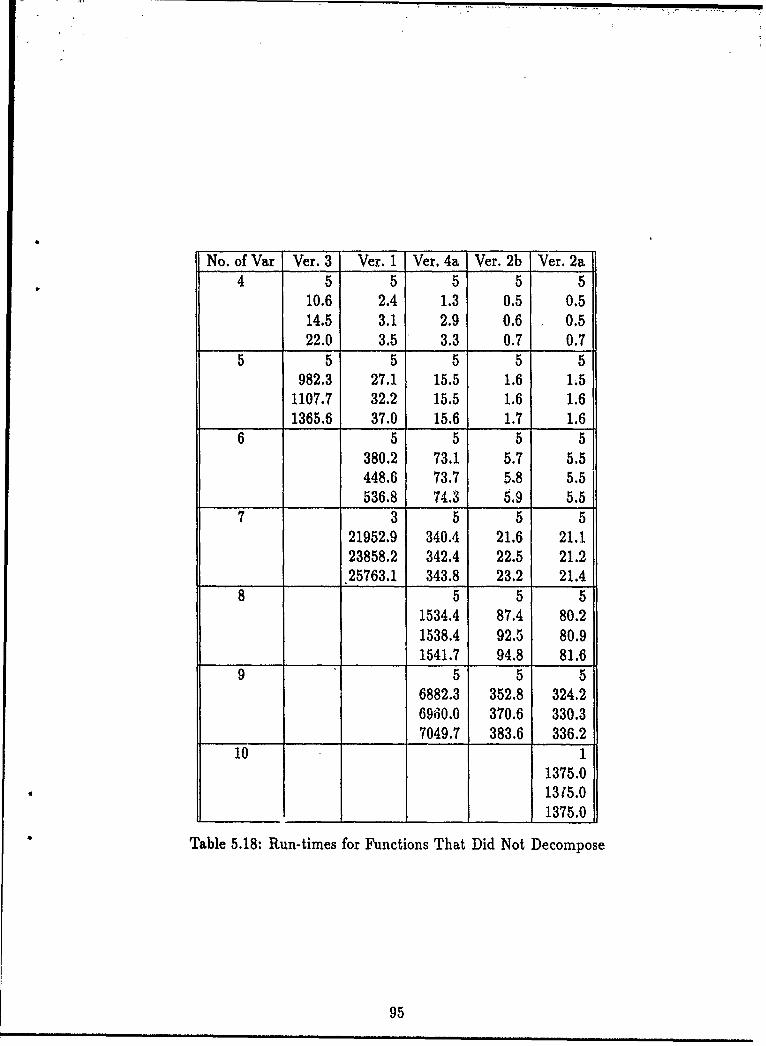
No. of Var Vet. 3 Vet. 1 Vet. 4a Ver. 2b Ver. 2a4 5 5 5 5 5

10.6 2.4 1.3 0.5 0.514.5 3.1 2.9 0.6 0.522.0 3.5 3.3 0.7 0.7

5 5 5 5 5 5982.3 27.1 15.5 1.6 1.5

1107.7 32.2 15.5 1.6 1.61365.6 37.0 15.6 1.7 1.6

6 5 5 5 5380.2 73.1 5.7 5.5448.6 73.7 5.8 5.5536.8 74.3 5,9 5.5

7 3 5 5 521952.9 340.4 21.6 21.123858.2 342.4 22.5 21.225763.1 343.8 23.2 21.4

8 5 5 51534.4 87.4 80.21538.4 92.5 80.91541.7 94.8 81.6

9 5 5 56882.3 352.8 324.26960.0 370.6 330.37049.7 383.6 336.2

10 11375.01315.01375.0

Table 5.18: Run-times for Functions That Did Not Decompose

95

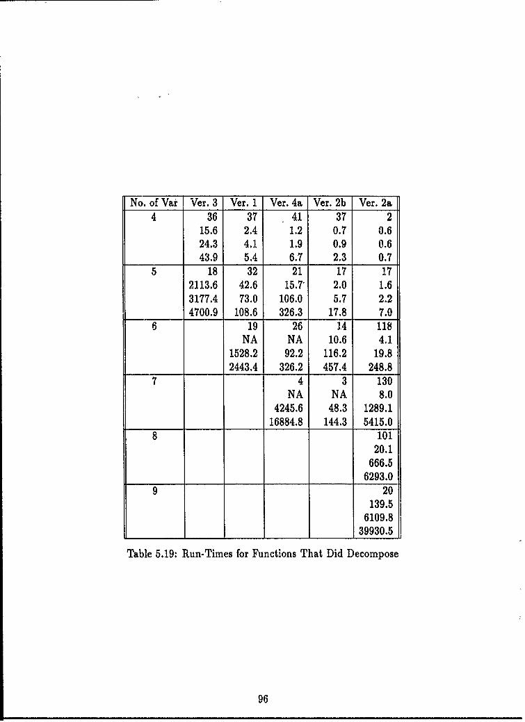
No. of Var Vet. 3 Vet. 1 Ver. 4a Ver. 2b Ver. 2a4 36 37 41 37 2

15.6 2.4 1.2 0.7 0.624.3 4.1 1.9 0.9 0.643.9 5.4 6.7 2.3 0.7

5 18 32 21 17 172113.6 42.6 15.71 2.0 1.63177.4 73.0 106.0 5.7 2.24700.9 108.6 326.3 17.8 7.0

6 19 26 .4 118NA NA 10.6 4.1

1528.2 92.2 116.2 19.82443.4 326.2 457.4 248.8

7 4 3 130NA NA 8.0

4245.6 48.3 1289.116884.8 144.3 5415.0

8 10120.1

666.56293.0

9 20139.5

6109.839930.5

Table 5.19: Run-Times for Functions That Did Decompose

96

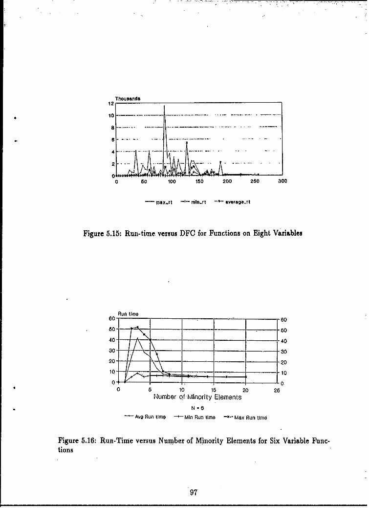
Thousands12

01

4

00 50 100 156 200 250 300

-- axjtt -m- nnrt -*0- average..rt

Figure 5.15; Run-time versus DFC for Functions on Eight Variables

Run time6001 ____ _0 __

30- -3

20- 2

*0 6 10 16 20 26N~umber oFflority Elements

Avg Run time --i- Min Run time -*- Max Run time

Figure 5.16: Run-Timne versus Number of Minority Elements for Six Variable Func-tions

97

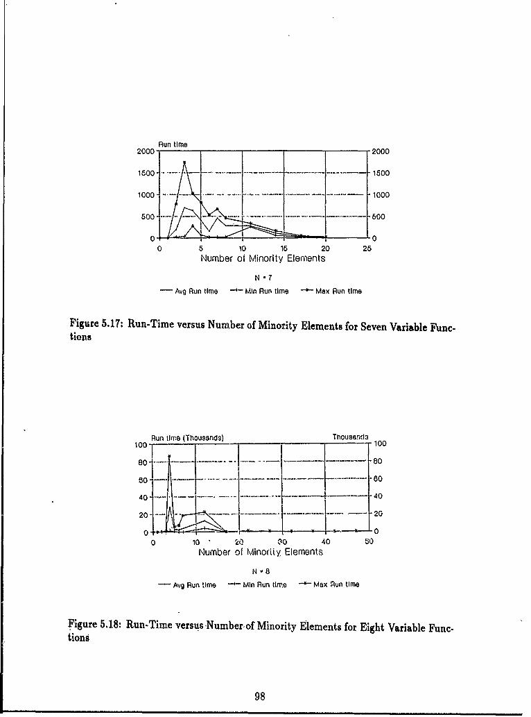
Run time2000 2000

1600.- " - --.. ........ .. .. ........... .. . 1500

1000 .. . . ....... . . ....... ... .. ..- 1000

500' 6 ---- - -. . . ....... 00

0 '00 5 10 15 20 25

Number of Minority Elements

N -7- Avg Run time *- Min Run time -* Max Run time

Figure 5.17: Run-Time versus Number of Minority Elements for Seven Variable Func-tions

Run time (Thousands) Thousand3100 -100

40 4020 ....... !20

0 10 20 $0 40 50Number of Minoriiy Elements

N -8

Avg Run time - Min Run time - Max Pul time

Figure 5.18: Run-Time versus Numberof Minority Elements for Eight Variable Func-tions

98

will be very close to the expected run-time for any unpatterned function.

5.4.3 Summary

There was little difference in the average DFC performance between versions. Thereare cases though with substantial differences. There was a lot of difference in theaverage run-time between versions. We narrowed the number of versions to the fivebest, a set of versions where an increase in average run-time always corresponded toan increase in cost reduction performance. The experimental run-time data was con-sistent with the expected exponential relationship between run-time and the numberof variables. There is a great deal of run-time sensitivity to the number of minorityelements in a function. Even the faster versions had sufficient cost reduction perfor-mance to allow for some interesting results in the Pattern Phenomenology experiments(Chapter 6).

5.5 Summary

This chapter introduces the problem of function decomposition and discussed the Adaimplementation that was used in this project. Approaches to decomposition consistof a test for decomposability and a search methodology. The test for decomposabilityis understood theoretically and is described in detail. The approaches to searchinghave little theoretical basis. We described several approaches that were experimentedwith in this project. We found that a 1 MIPS machine is capable of decomposingmost functions on less than 10 binary variables in a matter of hours.

99

Chapter ,

Pattern PhenomenQlogy

whqeA you, can, measure, what you are, speaking alkout, and express itin numbes, yq, know soz, thing about it;, but wkeq you cannot expressit nu r you~ lkNedge is; oa meager, aud unsatisfactory kind.'.",

- Lord Kelin.

6.1 Introduc t ionThis chapter hias tywoobjectites. On le one hand we experinentaly test our- ass ertioAthat Decompoqed Fuctig, C ardinality, (DFC,) a yery general zneas.v e of, p ttern-ness. On. the other hand,, assuming that DFC is a general nwasure. 9f- pttern-ness,we begin sizing up, the w9rld relative, to this new metric.

The first Qbjective is complementaryt9 the Chapter 4 theoretical 0me~iostratioAof DFO's generality., In Chap, t.r. 4 we r¢ated DF. to, the Isual measures oftcomputa-tional complexity; informati0on theoretic program length, algorithmic time complexity,and circuit size qomplexity.,

This chapter reports pattern-ness mraqsurements for many different kinds of things.These experiments are viewed in, a'yi analogous to the first experiments with othe;scientific instruments., For examp1e the first uses of' the mxrcury expaAsion ther-mometer were, qtj the s.me titre, aessing the ;eaqonableness of the tqn p.eraturereadings .nd quatifying. fo;, the st ti e yrious important temper.tures (_g, melt-ing points). The aknalogy. ext d4s to tfe difference between per eiyed teperatureand actual tempera ture. 'eTevmperature" ' first became a concept based on thi generalsensation of warmth ,qA cold. It only he came a precise objective physial p, qpertyafter the invention 9f a the mo ieter. We pw accept that any dfferencs, betweensensed an4d measured temp.grqures are due to 'th.ermal illusions" rater than spomefailing of thermometers. While we insist t hat a temperature measuring device reflectgeneral trendg in sseed tlmp.prature we expect situations were there are difererles.When we are cold, things, seem to he warmer than a thermometer would indicate.Therefore, a thermometer, is not ikn exac predict9r of sensed temperature. However,we would not accept a thermometer as, a measure of temperature if it got too, far

from our expectations. We think of DFC as a measure of pattern-ness much likea thermometer is a measure of temperature. We expect "pattern illusions" of twokinds. First there will be functions that are patterned whose pattern-ness is of a kindthat we do not appreciate. Thinking now in terms of the pattern-ness of an imageas compared to the DFC of the function that generates the image, some patternedfunctions (e.g. the prime number acceptor) will not look patterned to us. A secondpattern illusion might result from our tendency to impose a certain degree of order onthings. For example, people can see a face in almost any image with two horizontallydisplaced dark spots. As more specific examples, reference Figure 6.13 and 6.17; notethat character 31 of font 3 looks patterned but does not have low DFC; character 48of font 2 with permuted variables does not look patterned but has low DFC.

There are a few complicating factors in these experiments. For one thing wecannot be sure that the AFD program has found the true minimum cost. Most of theruns reported in this chapter were done with version 2a, the balance were done withversion 4a. As indicated in Chapter 5 we do not think we are missing the optimumby very much, but there is certainly some bias on the measured DFC as compared tothe true minimum DFC. Also, as discussed in Chapter 4, DFC does not include thecosts of interconnections. Therefore, things that decompose but do so with high DFCmay not be patterned at all. Finally, the AFD program's run-time is exponential inthe number of input variables. Therefore, we are limited to measuring the DFC offunctions with no more than about ten variables.

6.2 Randomly Generated Functions

6.2.1 Introduction

Patterned functions are both extremely rare and extremely common. If you look at allfunctions and choose a function at random, assuming all functions are equally likely,then the function almost certainly will not be patterned. Have you ever noticedthat if you watch a television that is not receiving a signal that realistic imagesnever seem to appear? If what we are seeing is a truly random image then anyparticular realistic image (e.g. John Wayne sitting on a horse) is just as probableas any particular random looking image. You can watch these random images fora long time and, although some strange psychological phenomena start to happen,you never see anything that is remotely realistic. Realistic images are patterned andpatterns are extremely rare in the space of all functions. On the other hand if youpick realistic functions, such as functions with names (e.g. addition, sine, palindromeacceptor), real images, real sounds, etc. then the function almost certainly will bepatterned. That is, patterns are extremely common in the real world. It seems to usthat this is a physical property of the world, kind of like mass or any other physicalproperty.

This section will assess the cost distribution (mean, maximum, minimum, andoccasionally standard deviations) for arbitrary functions, functions with a specific

102

number of minority, element.s,, and functions with a specific number of cares. Thisassessment will be. based on theoretical and, experimental results.

6.2.2 Completely Random Functions

This section is concerned with the cost of completely random functions. That is', theclass of functions to be considered includes all functions and each function has thesame probability of being chosen as any other function. Of course these functions are"random!' only in the sense that generating a function using- a random source of O'sand l's is one way of generating a sample of this class. All the functions in this classare completely deterministic. That is, they all produce a specific output for a specificinput. Later sections will limit class membership to those functions with a specificnumber of minority elements or a specific number of cares.

We need some initial results that will allow us to characterize the number offunctions with respect to DFC.

Theorem 6.1 The minimum DFC of a function is either 0, 2, or a sum of powersof 2 greater than 2.,

Proof:DFC is a sum of powers of 2 by definition. If a minimum representation has costgreater than 2 and an individual component of cost 2 then we must have a situationwhere the component of cost 2 (pl) is connected to another component (p2). There-fore, P2 could be redefined without increasing P2's cost such that P, is not required.The representation with the redefined P2 would have lower cost than the original rep-resentation which contradicts the assumption that we began with a minimum costrepresentation. Therefore, the assumption that we can have a minimum cost repre-sentation with a component of cost 2 is false.01

Theorem 6.2 An integer n is the sum of powers of 2 greater than 2 if and only if nis evenly divisible by 4.

Proof:

Assume that n is the sum of powers of 2 greater than 2, i.e. n = P 2 where eachpi 2 2. Thus, n = 4 t=I 2P-2 where pi - 2 > 0. The sum is a whole number qinceeach of the terms is a whole number. Thus, n is divisible by 4.

Assume that n is divisible by 4, i.e. there exists a whole number n' such that n = 4n'.

Thus n = 4.

103

Theorem 6.3 All functions must have DFC's of 0,..2, or multiples of 4.

Proof:Follows from Theorems 6.1 and 6.2.0

Theorem 6.4 The maximum number of non-vacuous variables (n') for a functionwith DFC> 4 is n' = _.. + 1.

Proof:It follows from Theorem 6.5 that 4(n' - 1) is the minimum cost for n' non-vacuousvariables; that is n' < "-7 + 1. The equality follows since --T + 1 is always aninteger by Theorem 6.2.

Now we consider the number of functions of a given cost:

* cost = 0: There are n projection functions and 2 constant function for a totalof n + 2 functions of cost 0.

• cost = 2: There are n complements of the projection functions for a total of nfunctions of cost 2.

* cost = 4: There can only be .two non-vacuous variables by Theorem 6.4. Thereare n choose 2 (or n(n - 1)/2) pairs of variables. Let n' = 2. There are 22"'total functions on n' variables. Of these, n! + 2 have cost 0 and n' have cost2. By Theorem 6.3 above, no functions have cost 1 or 3. Therefore, there are22"' - (n'+ 2) - n' functions left of cost 4. Since n' = 2, 22"' - (n' + 2) - n' = 10.Therefore, there are 10n(n - 1)/2 functions of cost 4.

* Cost = 8: There can only be three non-vacuous variables. There are n choose3 (or n(n - 1)(n - 2)/6) triples of variables. Let n' = 3. There are 22"' totalfunctions on n' variables. Of these, n' + 2 have cost 0, nt' have cost 2 andlOn'(n' - 1)/2 functions of cost 4. By Theorem 6.3 above, no functions have

cost 1, 3, 5, 6 or 7. Therefore, there are 22" ' - (n' + 2) - n' - 10n'(n' - 1)/2

functions left of cost 8. Since n' = 3, 22"' - (n' + 2) - n' - 10n'(n' - 1)/2 = 218.Therefore, there are 218n(n - 1)(n - 2)/6 functions of cost 8.

* Cost = 12: There can only be four non-vacuous variables. There are n choose4 (or n(n - 1)(n - 2)(n - 3)/24) groups of variables. Let n' = 4. There are22"' total functions on n' variables. Of these, n' + 2 have cost 0, n' have cost 2,10n'(n' - 1)/2 functions of cost 4 and 218n'(n' - 1)(n' - 2)/6 functions of cost8. By Theorem 6.3 above, no functions have cost 1, 3, 5, 6, 7, 9, 10, 11, 13,14, or 15. We do not know how many functions there are of cost 16, but we

104

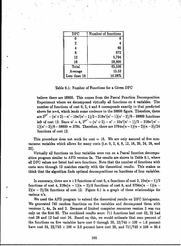
DFC Numbei of functions0 62 44 608 87212 5,79416 58,800

Total 65,536Average 15.53

Less than 16 10.28%

Table 6.1: Number of Functions for a Given DFC

believe there are 58800. This comes from the Pascal Function DecompositionExperiment where we decomposed virtually all functions on 4 variables. Thenumber of functions of cost 0, 2, 4 and 8 corresponds exactly to that predictedabove for n=4, which lends some credence to the 58800 figure. Therefore, there

are 22"' - (n' + 2) - n '- lOn'(n' - 1)/2 - 218n'(n'- 1)(n'- 2)/6-58800 functions

left of cost 12. Since n' = 4, 22n' - (n' + 2) - n' - lOn'(n' - 1)/2 - 218n'(n' -1)(n'- 2)/6 - 58800 = 5794. Therefore, there are 5794n(n - 1)(n - 2)(n - 3)/24functions of cost 12.

This procedure does not work for cost = 16. We are only assured of five non-vacuous variables which allows for many costs (i.e. 0, 2, 4, 8, 12, 16, 20, 24, 28, and32).

Virtually all functions on four variables were run on a Pascal function decompo-sition program similar to AFD version 2a. The results are shown in Table 6.1, whereall DFC values not listed had zero functions. Note that the number of functions withcosts zero through 12 matches exactly with the theoretical results. This makes usthink that the algorithm finds optimal decompositions on functions of four variables.

In summary, there are n + 2 functions of cost 0, n functions of cost 2, 10n(n - 1)/2functions of cost 4, 218n(n - 1)(n - 2)/6 functions of cost 8, and 5794n(n - i)(n -

2)(n - 3)/24 functions of cost 12. Figure 6.1 is a graph of these relationships forvarious n's.

We used the AFD program to extend the theoretical results on DFC histograms.We generated 745 random functions on five variables and decomposed them withversions 1, 4a, 2a and 3. Because of limited computer resources version 3 was runonly on the first 92. The combined results were: 711 functions had cost 32, 22 hadcost 28 and 12 had cost 24. Based on this, we would estimate that zero percent ofthe functions on five variables have cost 0 through 20, 12/745 x 100 = 1.6 percenthave cost 24, 22/745 x 100 = 3.0 percent have cost 28, and 711/745 x 100 = 95.4

105

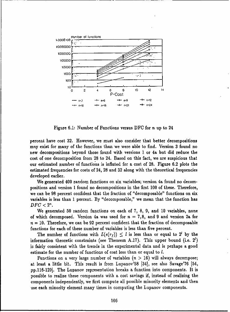
Number o lunctions

1.000E408 r10000000

002408 10020

P-Cost

- n,3 -4- n,6 -* n,9 ..-e.- n12

-'*- n,15 -+- n,18 - n,21 -.*- n,24

Figure 6.1: Number of Functions versus DFO for n up to 24

percent have cost 32. However, we must also consider that better decompositionsm~.y exist for many of the functions than we were able to find. Version 3 found nonew decompositions beyond those found with versions 1 or 4a but did reduce thecost of one decomposition from 28 to 24. Based on this fact, we are suspicious thatour estimated number of functions is inflated for a cost of 28. Figure 6.2 plots theestimated frequencies for costs of 24, 28 and 32 along with the theoretical frequenciesdeveloped earlier.

We generated 400 random functions on six variables; version 4a found no decom-positions and version 1 found no decompositions in the first 100 of these. Therefore,we can be 98 percent confident that the fraction of "decomposable" functions on sixvariables is less than 1 percent. By "decomposable," we mean that the function hasDFC < 2".

We generated 50 random functions on each of 7, 8, 9, and 10 variables, noneof which decomposed. Version 4a was used for n = 7, 8, and 9 and version 2a forn = 10. Therefore, we can be 92 percent confident that the fraction of decomposablefunctions for each of these number of variables is less than five percent.

The number of functions with L(e(rf)) <_ 1 is less than or equal to 2' by theinformation theoretic constraints (see Theorem A.17). This upper bound (i.e. 2')is fairly consistent with the trends in the experimental data and is perhaps a goodestimate for the number of functions of cost less than or equal to 1.

Funtions on a very large number of variables (n > 16) will always decompose;at least a little bit. This result is from Lupanov'58 134], see also Savage'76 [54,pp.116-120]. The Lupanov representation breaks a function into components. It ispossible to realize these components with a cost savings if, instead of realizing thecomponents independently, we first compute all possible minority elements and thenuse each minority element many times in computing the Lupanov components.

106

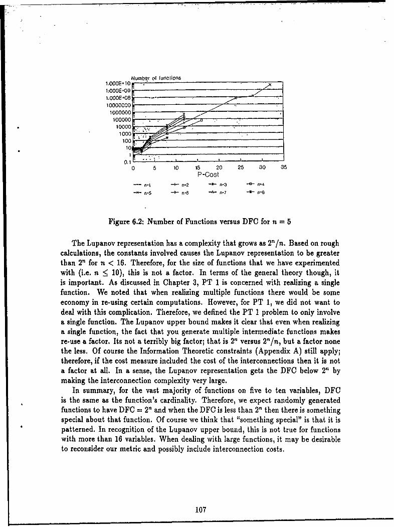
Number of functions1.000E410

1;000E+091.00OE+08100000001000000

10000010000

100010010

10.I

0 5 10 15 20 25 30 35

P-Cost-n- -+- n.2 2 n.7 .3-- n.4

n.S -8 A.-8 n.7 -I- '

Figure 6.2: Number of Functions versus DFC for n = 5

The Lupanov representation has a complexity that grows as 2"/n. Based on roughcalculations, the constants involved causes the Lupanov representation to be greaterthan 2n for n < 16. Therefore, for the size of functions that we have experimentedwith (i.e. n _ 10), this is not a factor. In terms of the general theory though, itis important. As discussed in Chapter 3, PT 1 is concerned with realizing a singlefunction. We noted that when realizing multiple functions there would be someeconomy in re-using certain computations. However, for PT 1, we did not want todeal with this complication. Therefore, we defined the PT 1 problem to only involvea single function. The Lupanov upper bound makes it clear that even when realizinga single function, the fact that you generate multiple intermediate functions makesre-use a factor. Its not a terribly big factor; that is 2n versus 2"/n, but a factor nonethe less. Of course the Information Theoretic constraints (Appendix A) still apply;therefore, if the cost measure included the cost of the interconnections then it is nota factor at all. In a sense, the Lupanov representation gets the DFC below 2n bymaking the interconnection complexity very large.

In summary, for the vast majority of functions on five to ten variables, DFCis the same as the function's cardinality. Therefore, we expect randomly generatedfunctions to have DFC = 2" and when the DFC is less than 2n then there is somethingspecial about that function. Of course we think that "something special" is that it ispatterned. In recognition of the Lupanov upper bound, this is not true for functionswith more than 16 variables. When dealing with large functions, it may be desirableto reconsider our metric and possibly include interconnection costs.

107

6.2.3 Functions with a Specific Number of Minority Ele-ments

Some functions have a definite minority in terms of output type. That is, a functionmay have 0 as its output for all but a small number of inputs. In this case we wouldsay that 1 is the minority output type. An element of a function with output of theminority type is calied a "minority element." This section will investigate the costof functions with respect to their number of minority elements. Functions with arelatively small fraction of minority elements are common in practice. For example,the prime number acceptor only outputs a 1 for the relatively few numbers that areprime and a target detection algorithm would only output a 1 on the extremely smallfraction of possible images that include targets.

There is a minimum cost for a function with a given number of non-vacuousvariables. In particular, if a function has n non-vacuous variables then the cost of thefunction cannot be less than 4(n - 1). Therefore, if a function on n variables has ivacuous variables the cost of this function is at least 4(n - i - 1).

Theorem 6.5 If F is the set of binary functions with n non-vacuous variables thenthe greatest lower bound on the cost of f E F is 4(n - 1).

Proof:There exists a function f in F with ni = 2 for i = 1,... , P where ni is the numberof input variables for component pi of the representation of f and P is the totalnumber of components in the representation. We are assured of f's existence sincefor any representation with a pi with ni > 3 we could partition the variables of piinto groups of size ni - 1 and 1 with cost 2"i- 1 + 22 which is less that 2 n for ni > 3.The resulting function would be an element of F since the composition of functionswhich are essentially dependent on all their inputs is a function that is essentiallydependent on all of its inputs. We can solve for P for such a representation since thetotal number of variables input to the pi's is the original n input variables plus the Pvariables generated by some pi minus the final output variable which is not an input.That is,

P

zni=n+P-1i=1

which reduces to P = n - 1 since all ni = 2. The cost of this representation is:P n-1

Z21 1 = 2 = 4(n- 1).

i1 i=I

This is a greatest lower bound since there exist functions with this cost, e.g. x, + x2 +... + x,, where + is an OR operation and the xi's are Boolean variables.0

There is a relationship between the number of minority elements in a functionand the possible existence of vacuous variables. Intuitively, if a function has an odd

108

number of minority elements then it is not possible for a partition matrix to have twoidentical sets of columns and two identical sets of columns are possible for a functionwith a vacuous variable. We state this as a theorem.

Theorem 6.6 Suppose F is the set of functions on n variables with exactly k minor-ity elements, where k is an integer greater than zero. There exists f E F such that fhas i vacuous variables if and only if k has 2i as a factor.

Proof:

f has k minority elements and i vacuous variables. If there are no vacuous variablesthen 20 is obviously a factor. Otherwise, choose a vacuous variable. The partitionmatrix with respect to this variable has two identical columns. Of course the columnscontain the same number of minority elements and therefore the total function had aneven number of minority elements. If we now drop this vacuous variable and repeatthe argument for the remaining function we see that there is a factor of 2 in k foreach vacuous variable.

Let k = k2'. We can construct an f with i vacuous variables one vacuous variable ata time. For the first vacuous variable, let f(... ,0, .. '.) = f(... ,1,...) but leave thespecific values undefined. Now consider f... ., 0,...) as the "function" and repeat theprocedure i times. This is possible since there are a multiple of 2' minority elements.The final "function" can be defined arbitrarily as long as it has k' minority elements.A function so constructed has i vacuous variables and k2' minority elements.0

This result could be used as a search constraint in the decomposition process. Forexample, if there are an odd number of minority elements then there is no point intesting for vacuous variables.

We now have a connection between the number of minority elements and thenumber of vacuous variables as well as between the number of vacuous variables andthe minimum cost.

Theorem 6.7 Let F be the set of binary functions on n variables with exactly kminority elements. Let i be the largest i such that 2' is a factor of k. Then for allf E F the cost of f is > 4(n - i' - 1) and there exists an f E F such that the cost off equals 4(n - i - 1). That is, the cost of functions in F has a greatest lower boundof 4(n - i' - 1).

Proof:This follows from Theorem 6.5 and Theorem 6.6.0

109

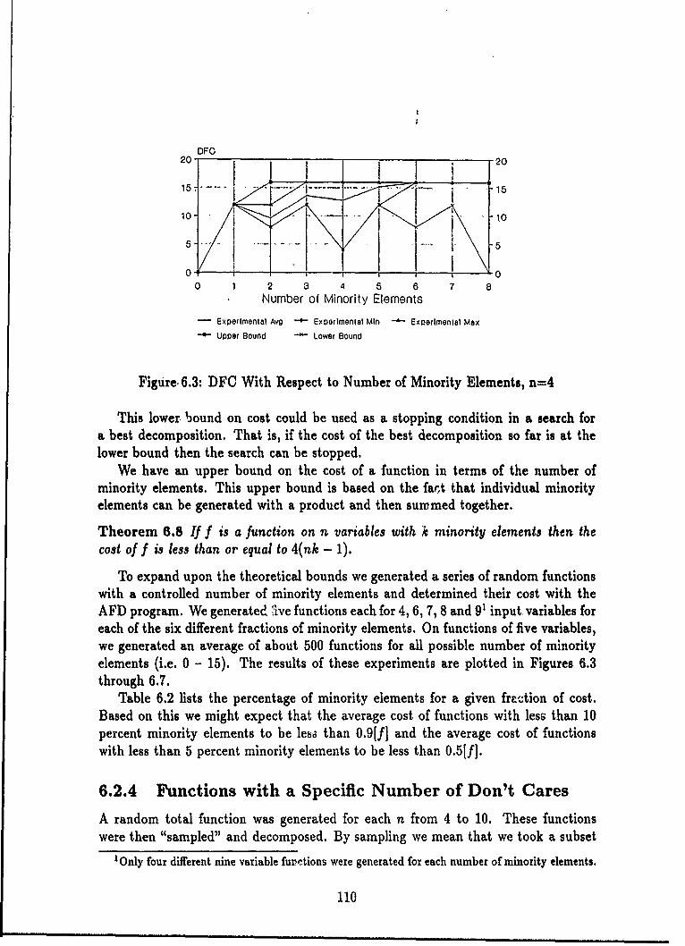
DFO20 20

10-0

0 0

0 1 2 a 5 6 7 8Number of Minority Elements

- Experimental Avg ,--Experimental Min -4 Experimental Max

--- Upper Bound - Lower Bound

Figure, 6.3: DFO With Respect to Number of Minority Elements, n=4

This lower bound on cost could be used as a stopping condition in a search fora best decomposition. That is, if the cost of the best decomposition so far is at thelower bound then the search can be stopped.

We have an upper bound on the cost of a function in terms of the number ofminority elements. This upper bound is based on the fact that individual minorityelements can be generated with a product and then summed together.

Theorem 6.8 If f is a function on n variables with k minority elements then thecost of f is less than or equal to 4(nk - 1).

To expand upon the theoretical bounds we generated a series of random functionswith a controlled number of minority elements and determined their cost with theAFD program. We generated ave functions each for 4, 6, 7, 8 and 9' input variables foreach of the six different fractions of minority elements. On functions of five variables,we generated an average of about 500 functions for all possible number of minorityelements (i.e. 0 - 15). The results of these experiments are plotted in Figures 6.3through 6.7.

Table 6.2 lists the percentage of minority elements for a given fraction of cost.Based on this we might expect that the average cost of functions with less than 10percent minority elements to be less than 0.9[f] and the average cost of functionswith less than 5 percent minority elements to be less than 0.5[f].

6.2.4 Functions with a Specific Number of Don't Cares

A random total function was generated for each n from 4 to 10. These functionswere then "sampled" and decomposed. By sampling we mean that we took a subset

'Only four different nine variable fuctions were generated for each number of minority elements.

110

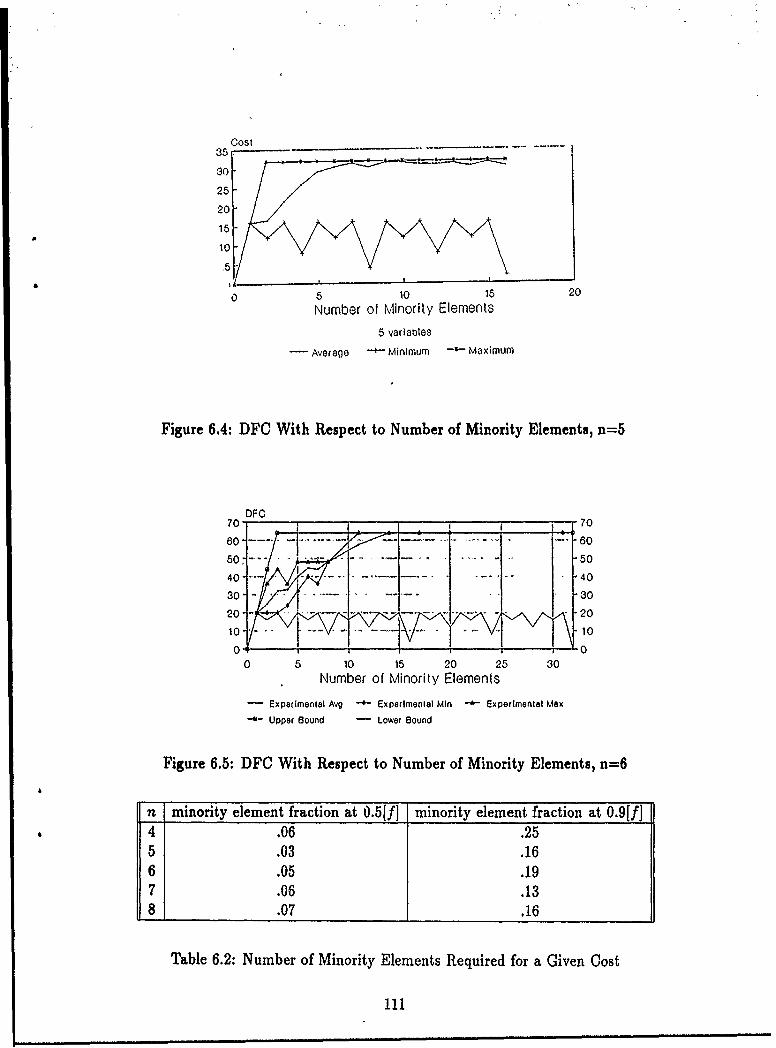
Cost

30

25

20-

15

10-

0 5 10 15 20Number of Minority Elements

5 VariableS

Average -4- Minimum *-w Maximum

Figure 6.4: DFO With Respect to Number of Minority Elements, n=5

DFO _ _ _ _ _ _ _ ___

70 7

00 --- --~- ---- 60

-50

40~ 40

20-- -20

10 0

0 5 10 15 20 25 30Number of Minority Elements

- Experimental Avg - Experimental Min -- Experimental Max-- Upper Bound -Lower Bound

Figure 6.5: DFC With Respect to Number of Minority Elements, n=6

n I minority element fraction at 0.5[fJ minority element fraction at 0.91f]4 .06 .255 .03 .166 .05 .197 .06 .138 .07 .16

Table 6.2: Number of Minority Elements Required for a Given Cost

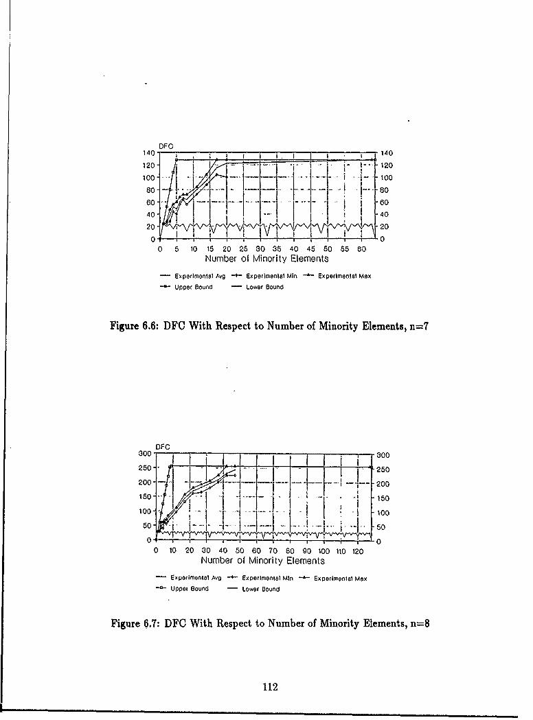
DFO140- _140

120- 1--, - 120

100- 100~

. . . 8

60 .- 60

40' 40

i " I i i .... 020-v2

o 0

0 5 10 15 20 25 3O 35 40 45 50 55 60Number of Minority Elements

- Experimental Avg "-- Experimental Min -6- Experimental Max

*- Upper Bound - Lower Bound


DFC300 -. 00200.. ... . . 2 - 00

250-- A 1 50

100 .. . . . . .. . 100150 50

0 10 20 30 40 50 60 70 80 90 100 110 120

Number of Minority Elements

- Expoilmental Avg -- Experimental MIn -- Experimental Max

-4-- Upper Bound - Lower Bound


112

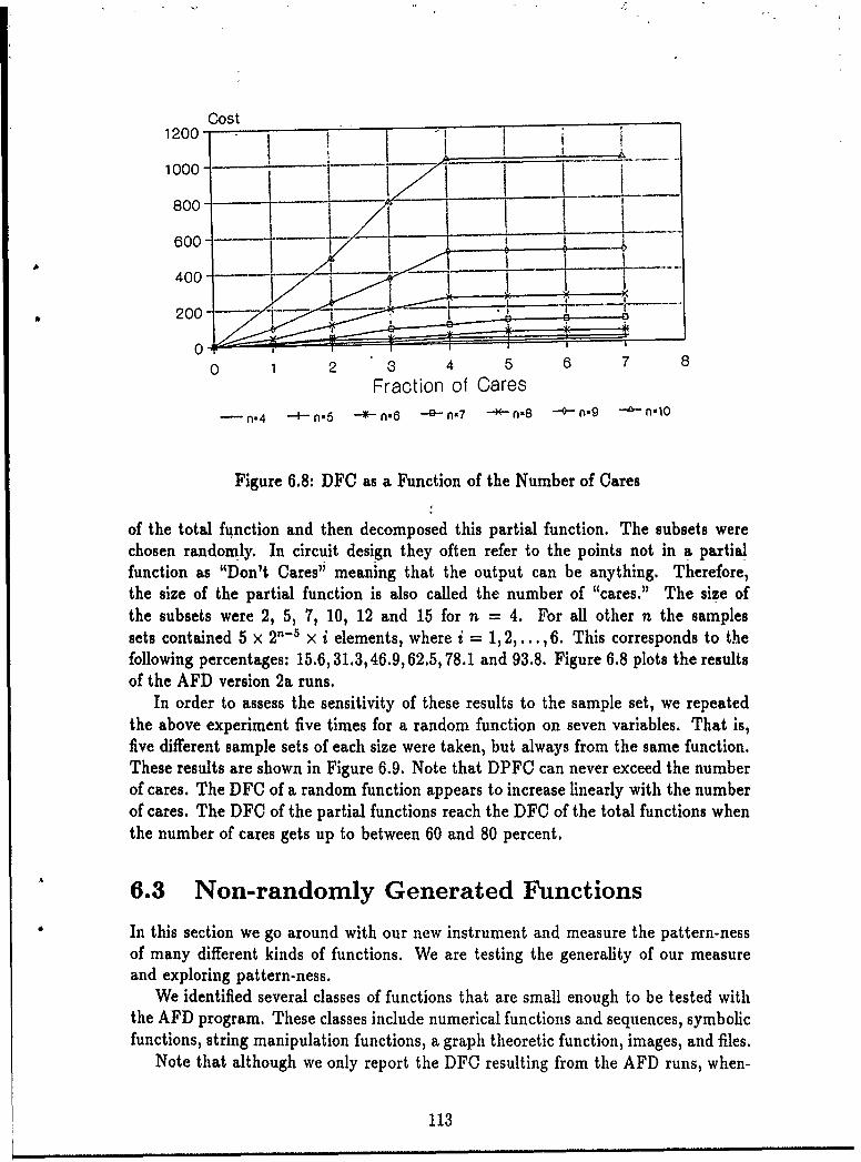
Cost1200 I

iooo___ I

1 I .. .100--- II800- -1

_ _ _

400-

200-

0- 0 123 4 5 7 8

Fraction of Caresn-4 --4- n.6 n-6 ae n-7 M n-8 --- n-9 n-lO

Figure 6.8: DFC as a Function of the Number of Cares

of the total function and then decomposed this partial function. The subsets werechosen randomly. In circuit design they often refer to the points not in a partialfunction as "Don't Cares' meaning that the output can be anything. Therefore,the size of the partial function is also called the number of "cares." The size ofthe subsets were 2, 5, 7, 10, 12 and 15 for n = 4. For all other n the samplessets contained 5 x 2n- 5 x i elements, where i = 1,2,...,6. This corresponds to thefollowing percentages: 15.6,31.3,46.9,62.5, 78.1 and 93.8. Figure 6.8 plots the resultsof the AFD version 2a runs.

In order to assess the sensitivity of these results to the sample set, we repeatedthe above experiment five times for a random function on seven variables. That is,five different sample sets of each size were taken, but always from the same function.These results are shown in Figure 6.9. Note that DPFC can never exceed the numberof cares. The DFC of a random function appears to increase linearly with the numberof cares. The DFC of the partial functions reach the DFC of the total functions whenthe number of cares gets up to between 60 and 80 percent.

6.3 Non-randomly Generated Functions

In this section we go around with our new instrument and measure the pattern-nessof many different kinds of functions. We are testing the generality of our measureand exploring pattern-ness.

We identified several classes of functions that are small enough to be tested withthe AFD program. These classes include numerical functions and sequences, symbolicfunctions, string manipulation functions, a graph theoretic function, images, and files.

Note that although we only report the DFC resulting from the AFD runs, when-

113

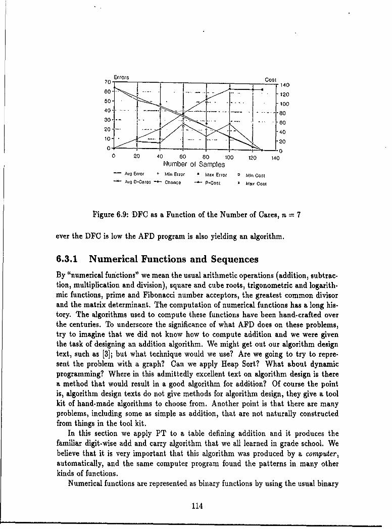
7 Er rors Cost14

60 1: -- - 12050- 100

10 - '20

O, 0o 20 40 60 80 100 120 140

Number of Samples- Avg Error + Min Error * Mex Error 1 Min Cost

Avg D-Cares + Chance - P-Cost I Max Cost

Figure 6.9: DFC as a Function of the Number of Cares, n - 7

ever the DFC is low the AFD program is also yielding an algorithm.

6.3.1 Numerical Functions and Sequences

By "numerical functions" we mean the usual arithmetic operations (addition, subtrac-tion, multiplication and division), square and cube roots, trigonometric and logarith-mic functions, prime and Fibonacci number acceptors, the greatest common divisorand the matrix determinant. The computation of numerical functions has a long his-tory. The algorithms used to compute these functions have been hand-crafted overthe centuries. To underscore the significance of what AFD does on these problems,try to imagine that we did not know how to compute addition and we were giventhe task of designing an addition algorithm. We might get out our algorithm designtext, such as [31; but what technique would we use? Are we going to try to repre-sent the problem with a graph? Can we apply Heap Sort? What about dynamicprogramming? Where in this admittedly excellent text on algorithm design is therea method that would result in a good algorithm for addition? Of course the pointis, algorithm design texts do not give methods for algorithm design, they give a toolkit of hand-made algorithms to choose from. Another point is that there are manyproblems, including some as simple as addition, that are not naturally constructedfrom things in the tool kit.

In this section we apply PT to a table defining addition and it produces thefamiliar digit-wise add and carry algorithm that we all learned in grade school. Webelieve that it is very important that this algorithm was produced by a computer,automatically, and the same computer program found the patterns in many otherkinds of functions.

Numerical functions are represented as binary functions by using the usual binary

114

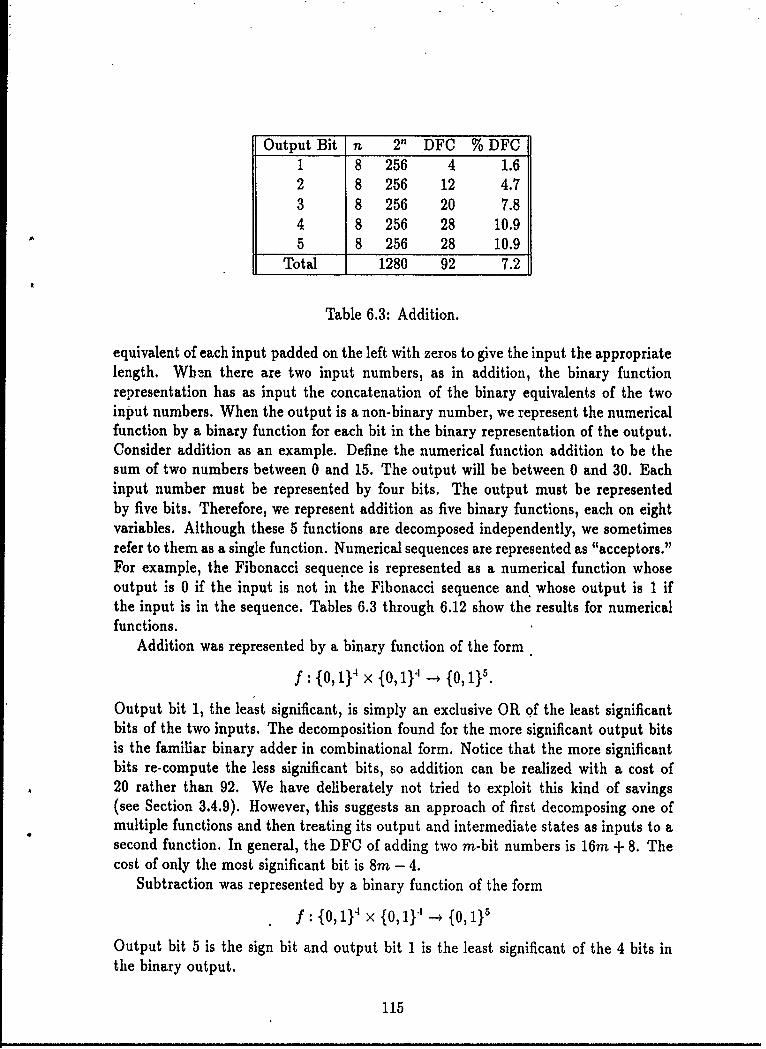
Output Bit n 2" DFC % DFC1 8 256 4 1.62 8 256 12 4.73 8 256 20 7.84 8 256 28 10.95 8 256 28 10.9

Total 1280 92 7.2

Table 6.3: Addition.

equivalent of each input padded on the left with zeros to give the input the appropriatelength. Wb-In there are two input numbers, as in addition, the binary functionrepresentation has as input the concatenation of the binary equivalents of the twoinput numbers. When the output is a non-binary number, we represent the numericalfunction by a binary function for each bit in the binary representation of the output.Consider addition as an example. Define the numerical function addition to be thesum of two numbers between 0 and 15. The output will be between 0 and 30. Eachinput number must be represented by four bits. The output must be representedby five bits. Therefore, we represent addition as five binary functions, each on eightvariables. Although these 5 functions are decomposed independently, we sometimesrefer to them as a single function. Numerical sequences are represented as "acceptors."For example, the Fibonacci sequence is represented as a numerical function whoseoutput is 0 if the input is not in the Fibonacci sequence and whose output is 1 ifthe input is in the sequence. Tables 6.3 through 6.12 show the results for numericalfunctions.

Addition was represented by a binary function of the form

f/: {o,114 X× ,11 {o,1 } .

Output bit 1, the least significant, is simply an exclusive OR of the least significantbits of the two inputs. The decomposition found for the more significant output bitsis the familiar binary adder in combinational form. Notice that the more significantbits re-compute the less significant bits, so addition can be realized with a cost of20 rather than 92. We have deliberately not tried to exploit this kind of savings(see Section 3.4.9). However, this suggests an approach of first decomposing one ofmultiple functions and then treating its output and intermediate states as inputs to asecond function. In general, the DFC of adding two m-bit numbers is 16m + 8. Thecost of only the most significant bit is 8m - 4.

Subtraction was represented by a binary function of the form

f: fo,) × X 0 14-4o, 1}

Output bit 5 is the sign bit and output bit 1 is the least significant of the 4 bits inthe binary output.

115

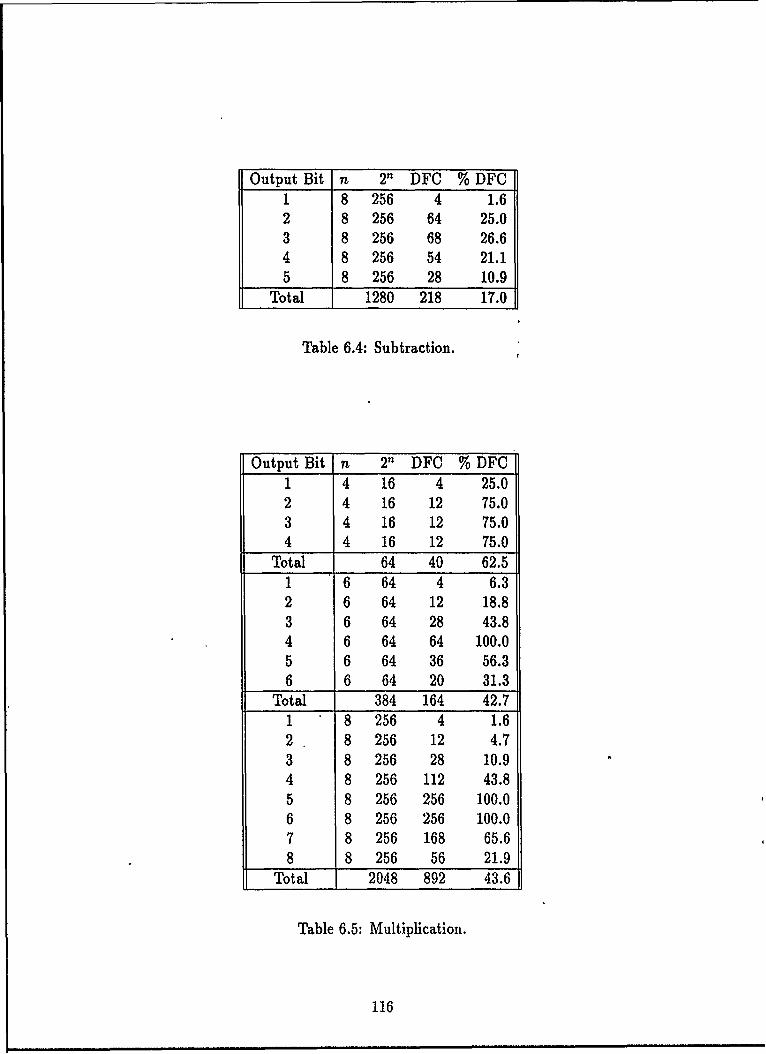
Output Bit n 2n DFC % DFC1 8 256 4 1.62 8 256 64 25.03 8 256 68 26.64 8 256 54 21.15 8 256 28 10.9

Total 1280 218 17.0

Table 6.4: Subtraction.

Output Bit n 2n DFC % DFC1 4 16 4 25.02 4 16 12 75.03 4 16 12 75.04 4 16 12 75.0

Total 64 40 62.51 6 64 4 6.32 6 64 12 18.83 6 64 28 43.84 6 64 64 100.05 6 64 36 56.36 6 64 20 31.3

Total 384 164 42.71 8 256 4 1.62 8 256 12 4.73 8 256 28 10.94 8 256 112 43.85 8 256 256 100.06 8 256 256 100.07 8 256 168 65.68 8 256 56 21.9

Total 2048 892 43.6

Table 6.5: Multiplication.

116

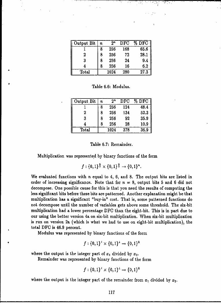
Output Bit n 2" DFC % DFC1 8 256 168 65.62 8 256 72 28.13 8 256 24 9.44 8 256 16 6.2

Total 1024 280 27.3

Table 6.6: Modulus.

Output Bit n 2n DFC % DFC1 8 256 124 48.42 8 256 134 52.33 8 256 92 35.94 8 256 28 10.9

Total 1024 378 36.9

Table 6.7: Remainder,

Multiplication was represented by binary functions of the form

f: {0,1}, x {0,1} -, {o,1}-.

We evaluated functions with n equal to 4, 6, and 8. The output bits are listed inorder of increasing significance. Note that for n = 8, output bits 5 and 6 did notdecompose. One possible cause for this is that you need the results of computing theless significant bits before these bits are patterned. Another explanation might be thatmultiplication has a significant "buy-in" cost. That is, some patterned functions donot decompose until the number of variables gets above some threshold. The six-bitmultiplication had a lower percentage DFC than the eight-bit. This is in part due toour using the better version 4a on six-bit multiplication. When six-bit multiplicationis run on version 2a (which is what we had to use on eight-bit multiplication), thetotal DFC is 46.9 percent.

Modulus was represented by binary functions of the form

f: {0,1}' X {o,1}4 -f {0,1 18

where the output is the integer part of x, divided by X2 .Remainder was represented by binary functions of the form

f: o, 1}' X f0, 11 -+ {0, 118

where the output is the integer part of the remainder from x1 divided by X2 .

117

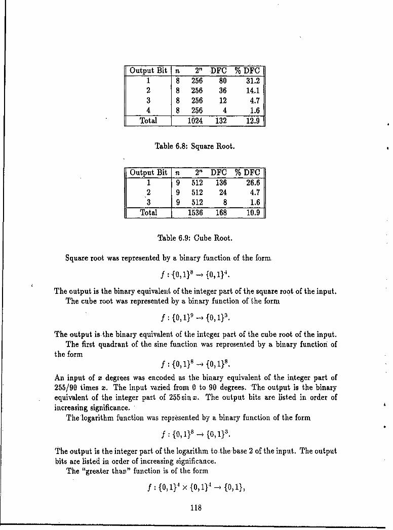
Output Bit n 2n -DFC % DFC1 8 256 80 31.22 8 256 36 14.13 8 256 12 4.74 8 256 4 1.6

Total 1024 132 12.9

Table 6.8: Square Root.

Output Bit n 2" DFC % DFC1 9 512 136 26.62 9 512 24 4.73 9 512 8 1.6

Total 1536 168 10.9

Table 6.9: Cube Root.

Square root was represented by a binary function of the form.

:,{O, 18 -, ,14 .

The output is the binary equivalent of the integer part of the square root of the input.The cube root was represented by a binary function ofi he form

f: {0,}- {01}3.

The output is~the binary equivalent of the integei part of the cube root of the input.The first quadrant of the sine function was represented by a binary function of

the formf: {0,1}8 _ {0,1}.

An input of x degrees was encoded as the binary equivalent of -the integer part of255/90 times x. The input varied from 0 to 90 degrees. The output is the binaryequivalent of the integer part of 255 sin x. The output bits are listed in order ofincreasing significance. -

The'logarithm function was represented by a binary function of the form

f: .{0, 1}8 __ {0,1}3 .

The output is the integer part of the logarithm to the-base 2 of the input. The outputbits are listed in order of increasing significance.

The "greater than" function is of the form

f : {o,1}" x {oi} - {0,1},

118

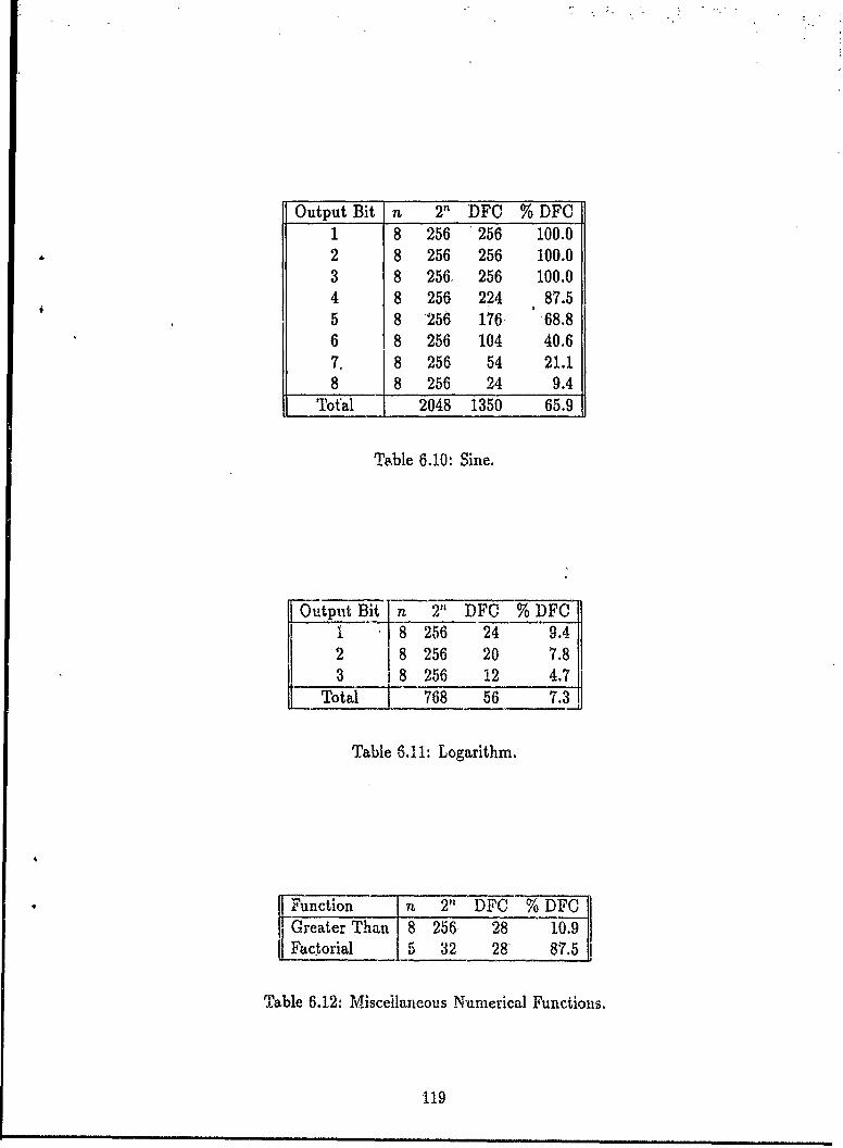
Output Bit n 2 n DFC % DFO1 8 256 '256 100.02 8 256 256 100.03 8 256. 256 100.04 8 256 224 87.55 8 '256 176- 68.86 8 256 104 40.67, 8 256 54 21.18 8 256 24 9.4

Tot'al 2048 1350 65.9

Table 6.10- Sine.

~Output Bit n 2" DFC % DFO1 8 256 24 9.4

2 8256 20 7.8 j3 8__ 256 12 4.7

1____ 768 56 7.3]

Table 6.11: Logarithm.

Function nz 2" DFO % DFCGreater Than 8 256, 28 10.9Factor ial 5 32 28- 87.5

Table 6.12: Miscellaneous Numerical Functions.

'119

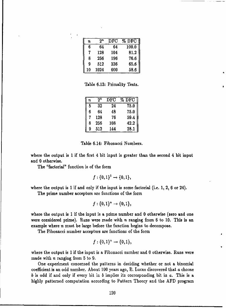
n 2n DFC %DFC6 64 64 100.07 128 104 81.28 256 196 76.69 512 336 65.6

10 1024 600 58.6

Table 6.13: Primality Tests.

n 2n DFC % DFC5 32 24 75.06 64 48 75.07 128 76 59.48 256 108 42.29 512 144 28.1

Table 6.14: Fibonacci Numbers.

where the output is 1 if the first 4 bit input is greater than the second 4 bit inputand 0 otherwise.

The "factorial" function is of the form

f : 101,1} 5 -- 0,1ill

where the output is 1 if and only if the input is some factorial (i.e. 1, 2, 6 or 24).The prime number acceptors are functions of the form

f,: {0,1}"' -- {0,1},

where the output is 1 if the input is a prime number and 0 otherwise (zero and onewere considered prime). Runs were made with n ranging from 6 to 10. This is anexample where n must be large before the function begins to decompose.

The Fibonacci number acceptors are functions of the form

f : fo0,1}_ f 0,1},

where the output is 1 if the input is a Fibonacci number and 0 otherwise. Runs weremade with n ranging from 5 to 9.

One experiment concerned the patterns in deciding whether or not a binomialcoefficient is an odd number. About 100 years ago, E. Lucas discovered that a chooseb is odd if and only if every bit in b implies its corresponding bit in a. This is ahighly patterned computation according to Pattern Theory and the AFD program

120

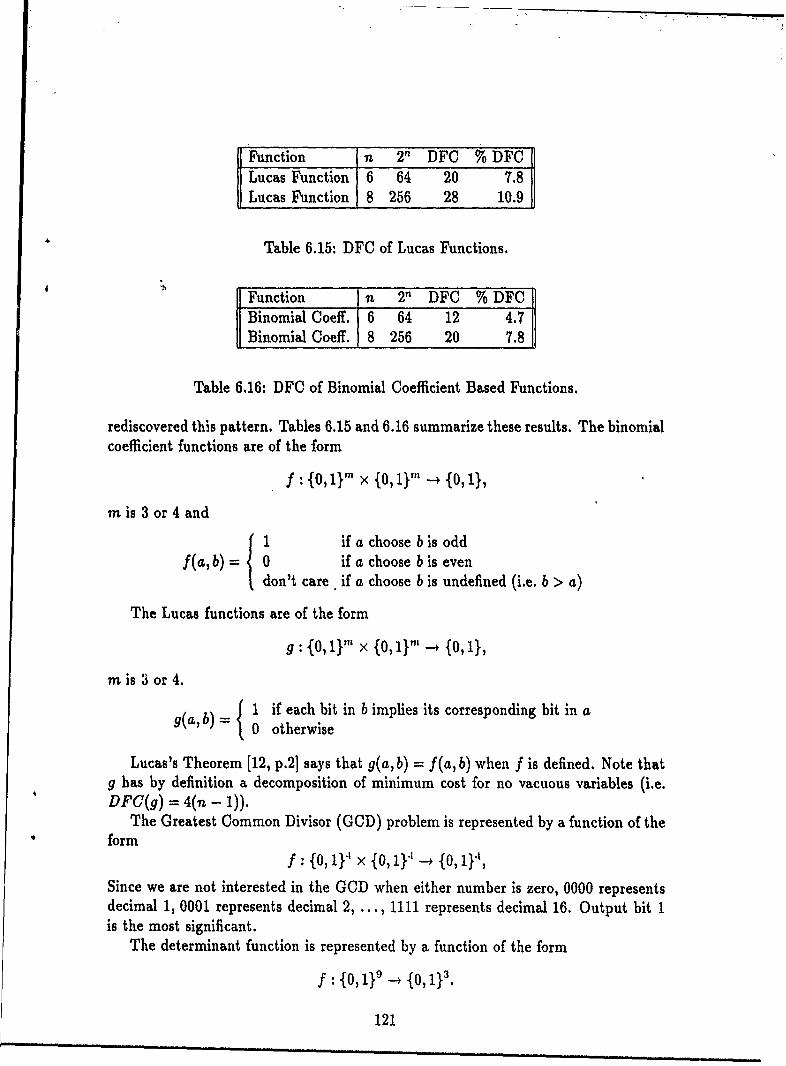
Function n 2n DFC % DFCLucas Function 6 64 20 7.8Lucas Function 8 256 28 10.9

Table 6.15: DFC of Lucas Functions.

Function 7n 2n DFC % DFCBinomial Coeff. 6 64 12 4.7Binomial Coeff. 8 256 20 7.8

Table 6.16: DFC of Binomial Coefficient Based Functions.

rediscovered this pattern. Tables 6.15 and 6.16 summarize these results. The binomialcoefficient functions are of the form

f : {0,J.} m X {0,iy -, 10,1},

m is 3 or 4 and { if a choose b is oddf(ab) 0 if a choose b is even

don't care if a choose b is undefined (i.e. b > a)

The Lucas functions are of the form

g : {0,1} m × {0,i}" -+ {0, 1,

m is 3 or 4.

b 1 if each bit in b implies its corresponding bit in ag(a,b)- = 0 otherwise

Lucas's Theorem [12, p.2] says that g(a, b) - f(a, b) when f is defined. Note thatg has by definition a decomposition of minimum cost for no vacuous variables (i.e.DFC(g) = 4(n - 1)).

The Greatest Common Divisor (GCD) problem is represented by a function of theform

f : {0, 114 X {o, 1141 {o, '},

Since we are not interested in the GCD when either number is zero, 0000 representsdecimal 1, 0001 represents decimal 2, ... , 1111 represents decimal 16. Output bit 1is the most significant.

The determinant function is represented by a function of the form

f : {0 -19_ {2,1}3.

121

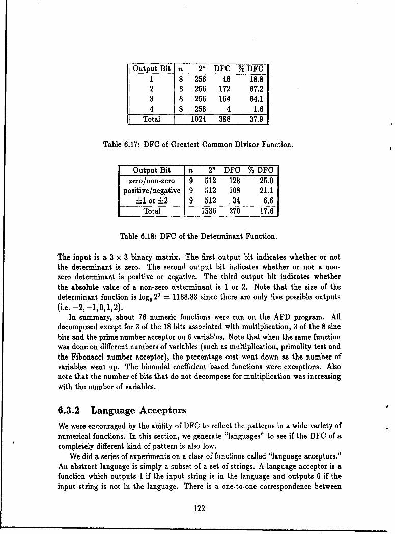
Output Bit n 2 n DFC % DFC1 8 256 48 18.82 8 256 172 67.23 8 256 164 64.14 8 256 4 1.6

Total 1024 388 37.9

Table 6.17: DFC of Greatest Common Divisor Function.

Output Bit n 2n DFC % DFCzero/non-zero 9 512 128 25.0

positive/negative 9 512 108 21.1±1 or ±2 9 512 .34 6.6

Total 1536 270 17.6

Table 6.18: DFC of the Determinant Function.

The input is a 3 x 3 binary matrix. The first output bit indicates whether or notthe determinant is zero. The second output bit indicates whether or not a non-zero determinant is positive or j egative. The third output bit indicates whetherthe absolute value of a non-zero 6tterminant is 1 or 2. Note that the size of thedeterminant function is log 5 2' = 1188.83 since there are only five possible outputs(i.e. -2,-i,0,1,2).

In summary, about 76 numeric functions were run on the AFD program. Alldecomposed except for 3 of the 18 bits associated with multiplication, 3 of the 8 sinebits and the prime number acceptor on 6 variables. Note that when the same functionwas done on different numbers of variables (such as multiplication, primality test andthe Fibonacci number acceptor), the percentage cost went down as the number ofvariables went up. The binomial coefficient based functions were exceptions. Alsonote that the number of bits that do not decompose for multiplication was increasingwith the number of variables.

6.3.2 Language Acceptors

We were encouraged by the ability of DFC to reflect the patterns in a wide variety ofnumerical functions. In this section, we generate "languages" to see if the DFC of acompletely different kind of pattern is also low.

We did a series of experiments on a class of functions called "language acceptors."An abstract language is simply a subset of a set of strings. A language acceptor is afunction which outputs 1 if the input string is in the language and outputs 0 if theinput string is not in the language. There is a one-to-one correspondence between

122

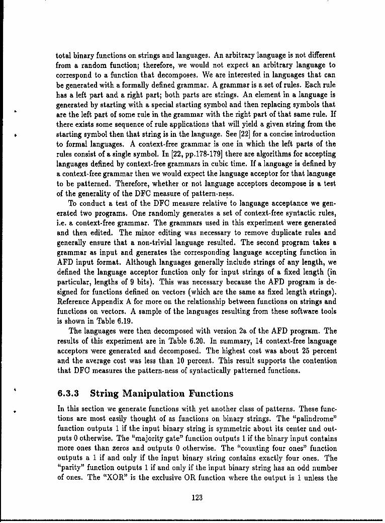
total binary functions on strings and languages. An arbitrary language is not differentfrom a random function; therefore, we would not expect an arbitrary language tocorrespond to a function that decomposes. We are interested in languages that canbe generated with a formally defined grammar. A grammar is a set of rules. Each rulehas a left part and a right part; both parts are strings. An element in a language isgenerated by starting with a special starting symbol and then replacing symbols thatare the left part of some rule in the grammar with the right part of that same rule. Ifthere exists some sequence of rule applications that will yield a given string from thestarting symbol then that string is in the language. See [22] for a concise introductionto formal languages. A context-free grammar is one in which the left parts of therules consist of a single symbol. In [22, pp.178-179] there are algorithms for acceptinglanguages defined by context-free grammars in cubic time. If a language is defined bya context-free grammar then we would expect the language acceptor for that languageto be patterned. Therefore, whether or not language acceptors decompose is a testof the generality of the DFC measure of pattern-ness.

To conduct a test of the DFC measure relative to language acceptance we gen-erated two programs. One randomly generates a set of context-free syntactic rules,i.e. a context-free grammar. The grammars used in this experiment were generatedand then edited. The minor editing was necessary to remove duplicate rules andgenerally ensure that a non-trivial language resulted. The second program takes agrammar as input and generates the corresponding language accepting function inAFD input format. Although languages generally include strings of any length, wedefined the language acceptor function only for input strings of a fixed length (inparticular, lengths of 9 bits). This was necessary because the AFD program is de-signed for functions defined on vectors (which are the same as fixed length strings).Reference Appendix A for more on the relationship between functions on strings andfunctions on vectors. A sample of the languages resulting from these software toolsis shown in Table 6.19.

The languages were then decomposed with version 2a of the AFD program. Theresults of this experiment are in Table 6.20. In summary, 14 context-free languageacceptors were generated and decomposed. The highest cost was about 25 percentand the average cost was less than 10 percent. This result supports the contentionthat DFC measures the pattern-ness of syntactically patterned functions.

6.3.3 String Manipulation Functions

In this section we generate functions with yet another class of patterns. These func-tions are most easily thought of as functions on binary strings. The "palindrome"function outputs 1 if the input binary string is symmetric about its center and out-puts 0 otherwise. The "majority gate" function outputs 1 if the binary input containsmore ones than zeros and outputs 0 otherwise. The "counting four ones" functionoutputs a 1 if and only if the input binary string contains exactly four ones. The"parity" function outputs 1 if and only if the input binary string has an odd numberof ones. The "XOR" is the exclusive OR function where the output is 1 unless the

123

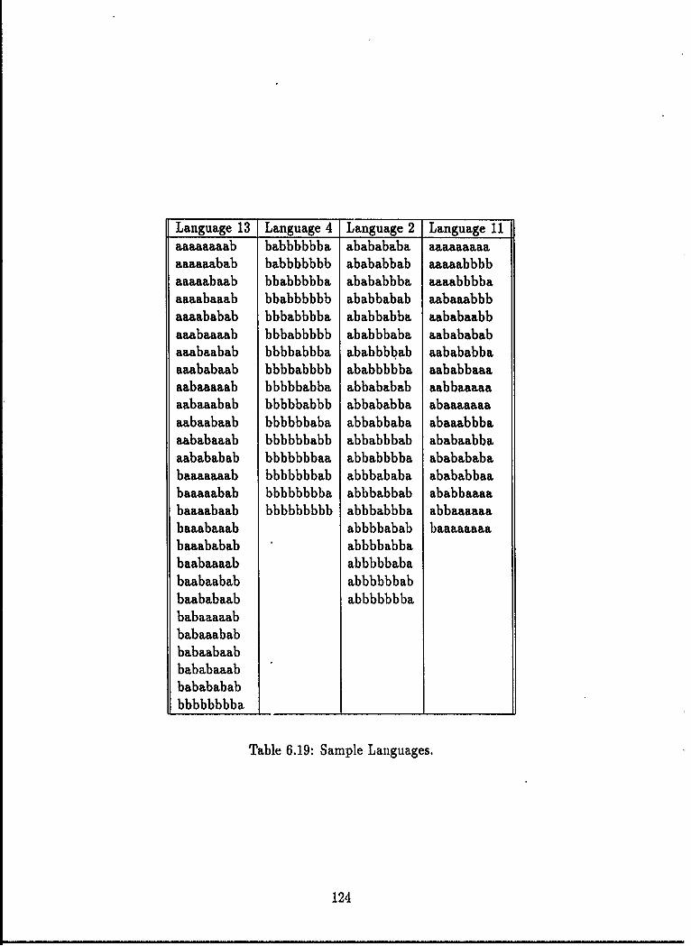
Language 13 Language 4 Language 2 Language 11aaaaaaaab babbbbbba ababababa aaaaaaaaaaaaaaabab babbbbbbb abababbab aaaaabbbbaaaaabaab bbabbbbba abababbba aaaabbbbaaaaabaaab bbabbbbbb ababbabab aabaaabbbaaaababab bbbabbbba ababbabba aababaabbaaabaaaab bbbabbbbb ababbbaba aababababaaabaabab bbbbabbba ababbbbab aabababbaaaababaab bbbbabbbb ababbbbba aababbaaaaabaaaaab bbbbbabba abbababab, aabbaaaaaaabaaabab bbbbbabbb abbababba abaaaaaaaaabaabaab bbbbbbaba abbabbaba abaaabbbaaababaaab bbbbbbabb abbabbbab ababaabbaaabababab bbbbbbbaa abbabbbba abababababaaaaaaab bbbbbbbab abbbababa abababbaabaaaaabab bbbbbbbba abbbabbab ababbaaaabaaaabaab bbbbbbbbb abbbabbba abbaaaaaabaaabaaab abbbbabab baaaaaaaabaaababab abbbbabbabaabaaaab abbbbbababaabaabab abbbbbbabbaababaab abbbbbbbababaaaaabbabaaababbabaabaabbababaaabbababababbbbbbbbba __________________

Table 6.19: Sample Languages.

124

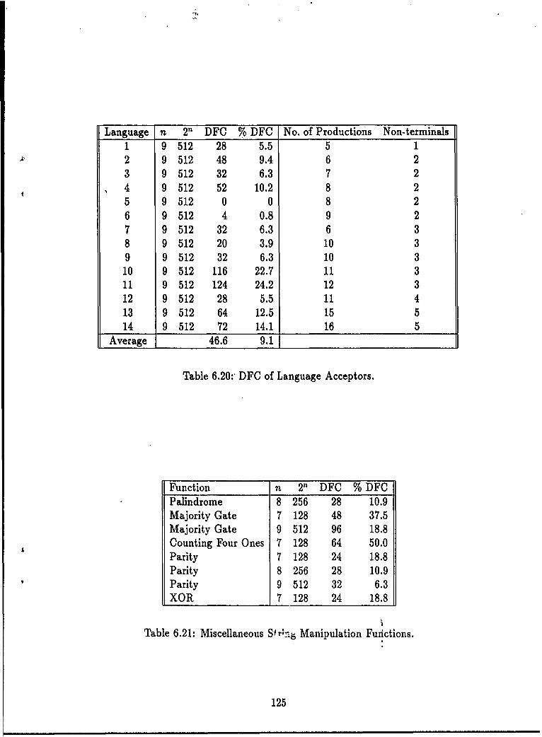
Language n 2" DFC % DFC No. of Productions Non-terminals1 9 512 28 5.5 5 12 9 512 48 9.4 6 23 9 512 32 6.3 7 24 9 512 52 10.2 8 25 9 512 0 0 8 26 9 512 4 0.8 9 27 9 512 32 6.3 6 38 9 512 20 3.9 10 39 9 512 32 6.3 10 310 9 512 116 22.7 11 311 9 512 124 24.2 12 312 9 512 28 5.5 11 413 9 512 64 12.5 15 514 9 512 72 14.1 16 5

Average 46.6 9.1

Table 6.20:- DFC of Language Acceptors.

Function n 2" DFC % DFCPalindrome 8 256 28 10.9Majority Gate 7 128 48 37.5Majority Gate 9 512 96 18.8Counting Four Ones 7 128 64 50.0Parity 7 128 24 18.8Parity 8 256 28 10.9Parity 9 512 32 6.3XOR 7 128 24 18.8

Table 6.21: Miscellaneous Sf r; Manipulation Fuiictions.

125

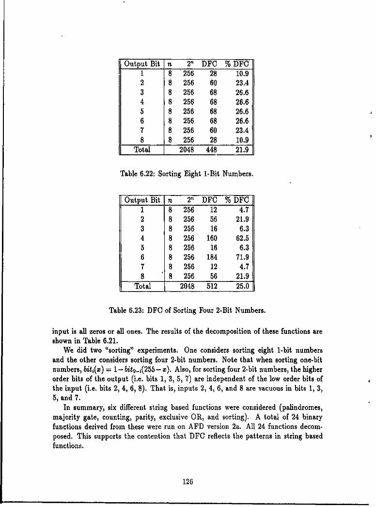
Output Bit n 2" DFC % DFC1 8 256 28 10.92 8 256 60 23.43 8 256 68 26.64 8 256 68 26.65 8 256 68 26.6

6 8 256 68 26.67 8 256 60 23.48 8 256 28 10.9

Total 2048 448 21.9

Table 6.22: Sorting Eight 1-Bit Numbers.

Output Bit n 2" DFC % DFC1 8 256 12 4.72 8 256 56 21.93 8 256 16 6.34 8 256 160 62.55 8 256 16 6.36 8 256 184 71.97 8 256 12 4.78 8 256 56 21.9

Total 2048 512 25.0

Table 6.23: DFC of Sorting Four 2-Bit Numbers.

input is all zeros or all ones. The results of the decomposition of these functions areshown in Table 6.21.

We did two "sorting" experiments. One considers sorting eight 1-bit numbersand the other considers sorting four 2-bit numbers. Note that when sorting one-bitnumbers, biti(x) = 1- bit 9 _i(255 - x). Also, for sorting four 2-bit numbers, the higherorder bits of the output (i.e. bits 1, 3, 5, 7) are independent of the low order bits ofthe input (i.e. bits 2, 4, 6, 8). That is, inputs 2, 4, 6, and 8 are vacuous in bits 1, 3,5, and 7.

In summary, six different string based functions were considered (palindromes,majority gate, counting, parity, exclusive OR, and sorting). A total of 24 binaryfunctions derived from these were run on AFD version 2a. All 24 functions decom-posed. This supports the contention that DFC reflects the patterns in string basedfunctions.

126

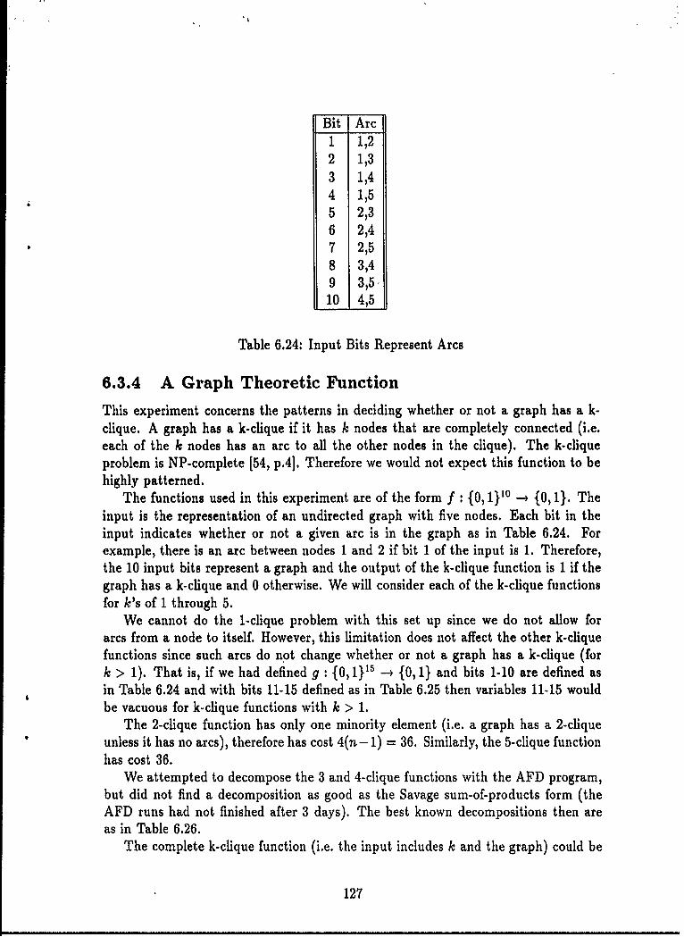
Bit Arc1 1,22 1,33 1,44 1,55 2,36 2,47 2,58 3,49 3,510 4,5

Table 6.24: Input Bits Represent Arcs

6.3.4 A Graph Theoretic Function

This experiment concerns the patterns in deciding whether or not a graph has a k-clique. A graph has a k-clique if it has k nodes that are completely connected (i.e.each of the k nodes has an arc to all the other nodes in the clique). The k-cliqueproblem is NP-complete [54, p.4]. Therefore we would not expect this function to behighly patterned.

The functions used in this experiment are of the form f : {0, 1}1° -* {0, 1}. Theinput is the representation of an undirected graph with five nodes. Each bit in theinput indicates whether or not a given arc is in the graph as in Table 6.24. Forexample, there is an arc between nodes 1 and 2 if bit 1 of the input is 1. Therefore,the 10 input bits represent a graph and the output of the k-clique function is 1 if thegraph has a k-clique and 0 otherwise. We will consider each of the k-clique functionsfor k's of 1 through 5.

We cannot do the 1-clique problem with this set up since we do not allow forarcs from a node to itself. However, this limitation does not affect the other k-cliquefunctions since such arcs do not change whether or not a graph has a k-clique (fork > 1). That is, if we had defined g : {0, 1}" -- {0, 1} and bits 1-10 are defined asin Table 6.24 and with bits 11-15 defined as in Table 6.25 then variables 11-15 wouldbe vacuous for k-clique functions with k > 1.

The 2-clique function has only one minority element (i.e. a graph has a 2-cliqueunless it has no arcs), therefore has cost 4(n- 1) = 36. Similarly, the 5-clique functionhas cost 36.

We attempted to decompose the 3 and 4-clique functions with the AFD program,but did not find a decomposition as good as the Savage sum-of-products form (theAFD runs had not finished after 3 days). The best known decompositions then areas in Table 6.26.

The complete k-clique function (i.e. the input includes k and the graph) could be

127

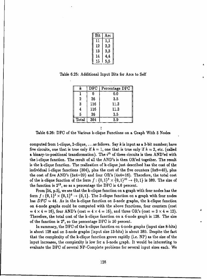
Bit Arc11 i,112 2,213 3,314 4,415 5,5

Table 6.25: Additional Input Bits for Arcs to Self

k DFC Percentage DFC1 0 0.02 36 3.53 116 11.34 116 11.35 36 3.5

Total 304 5.9

Table 6.26: DFC of the Various k-clique Functions on a Graph With 5 Nodes

computed from 1-clique, 2-clique, ... as follows. Say k is input as a 3-bit number; havefive circuits, one that is true only if k = 1, one that is true only if k = 2, etc. (calleda binary-to-positional transformation). The iLh of these circuits is then AND'ed withthe i-clique function. The result of all the AND's is then OR'ed together. The resultis the k-clique function. The realization of k-clique just described has the cost of theindividual i-clique functions (304), plus the cost of the five counters (5x8=40), plusthe cost of five AND's (5x4=20) and four OR's (4x4=16). Therefore, the total costof the k-clique function of the form f : {0, 1}' x {0, 1}O -. {0, 1} is 380. The size ofthe function is 213, so as a percentage the DFC is 4.6 percent.

From [54, p.5], we see that the k-clique function on a graph with four nodes has theform f : {0, 1}2 x {0, 1} -- {0., 1}. The 3-clique function on a graph with four nodeshas DFC = 44. As in the k-clique function on 5-node graphs, the k-clique functionon 4-node graphs could be computed with the above functions, four counters (cost= 4 x 4 = 16), four AND's (cost = 4 x 4 = 16), and three OR's (cost = 3 x 4 = 12).Therefore, the total cost of the k-clique function on a 4"-node graph is 128. The sizeof the function is 2s , so the percentage DFC is 50 percent.

In summary, the DFC of the k-clique function on 4-node graphs (input size 8-bits)is about 128 and on 5-node graphs (input size 13-bits) is about 380. Despite the factthat the complexity of the k-clique function grows rapidly (i.e. NP) as the size of theinput increases, the complexity is low for a 5-node graph. It would be interesting toevaluate the DFC of several NP-Complete problems for several input sizes each. We

128

k DFC Percentage DFC1 0 0.02 20 31.33 44 68.84 20 31.3

Total 84 32.8

Table 6.27: DFC of the Various k-clique Functions on a Graph With Four Nodes

Font Number Font Name Number of Characters0 default 2531 triplex 942 small 943 sans serif 954 Gothic 95

Table 6.28: Turbo Pascal V5.5 Font Sets

only have two data points on this single NP-Complete problem, but the growth incomplexity is much less than we expected. There are many long-standing unansweredquestions about the complexity of NP problems and decomposition may be an avenueto some new insights. In any case, DFC reflects the patterns in yet another context.

6.3.5 Images as Functions

In the preceding sections we saw that DFC captures the essential complexity of manykinds of functions. In this section, we consider the pattern-ness of images. Since DFCmeasures the pattern-ness of binary functions, we need to represent an image as abinary function. Suppose we want to assess the pattern-ness of a 16 pixel by 16 pixelblack and white image. We represent this image as a binary function of the form

f : {0, 1}n X {o, 1}m -4 {0, 1},

where n = 4 and m = 4. The first 4 bits of the input specify a column of the image,the last 4 bits specify a row and the output is the color (0 for white and 1 for black)of the pixel at that row a-Aid column.

This experiment uses a 16 by 16 pixel sampling of the characters generated byTurbo Pascal V5.52 for images. There are 631 total characters in 5 fonts, distributedas in Table 6.28. Each character was drawn on a VGA monitor With the maximumfont size that would allow all characters of a given font to fit within a 16 x 16 pixel

2Borland International.

129

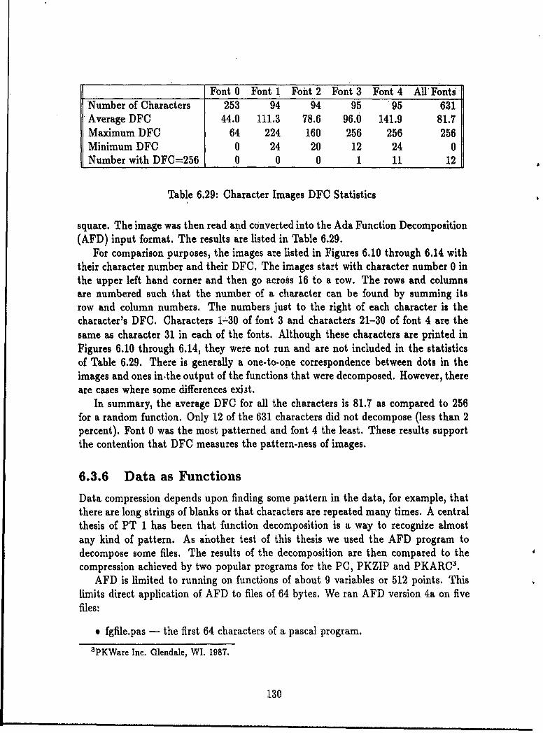
Font 0 Font 1 Font 2 Font 3 Font 4 All'Fonts''Number of Characters 253 94 94 95 95 631Average DFC 44.0 111.3 78.6 96.0 141.9 81.7Maximum DFC 64 224 160 256 256 256Minimum DFC 0 24 20 12 24 0Number with DFC-256 0 0 0 1 11 12

Table 6.29: Character Images DFC Statistics

square. The image was then read and converted into the Ada Function Decomposition(AFD) input format. The results are listed in Table 6.29.

For comparison purposes, the images are listed in Figures 6.10 through 6.14 withtheir character number and their DFC. The images start with character number 0 inthe upper left hand corner and then go across 16 to a row. The rows and columnsare numbered such that the number of a character can be found by summing itsrow and column numbers. The numbers just to the right of each character is thecharacter's DFC. Characters 1-30 of font 3 and characters 21-30 of font 4 are thesame as character 31 in each of the fonts. Although these characters are printed in'Figures 6.10 through 6.14, they were not run and are not included in the statisticsof Table 6.29. There is generally a one-to-one correspondence between dots in theimages and ones in.the output of the functions that were decomposed. However, thereare cases where some differences exist.

In summary, the average DFC for all the characters is 81.7 as compared to 256for a random function. Only 12 of the 631 characters did not decompose (less than 2percent). Font 0 was the most patterned and font 4 the least. These results supportthe contention that DFC measures the pattern-ness of images.

6.3.6 Data as Functions

Data compression depends upon finding some pattern in the data, for example, thatthere are long strings of blanks or that characters are repeated many times. A centralthesis of PT 1 has been that function decomposition is a way to recognize almostany kind of pattern. As another test of this thesis we used the AFD program todecompose some files. The results of the decomposition are then compared to thecompression achieved by two popular programs for the PC, PKZIP and PKARC'.

AFD is limited to running on functions of about 9 variables or 512 points. Thislimits direct application of AFD to files of 64 bytes. We ran AFD version 4a on fivefiles:

* fgfile.pas - the first 64 characters of a pascal program.

3PKWare Inc. Glendale, WI. 1987.

130

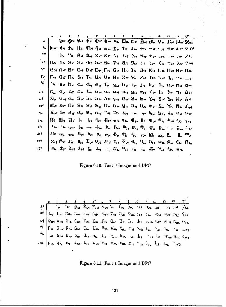
3 1/ (F 7 ' t to tf 2.. f2i74

14 # Ab tio!. q10~ §41 u~a~ t. 4&io -+vq 4-v ite +-4I' rh. q V 6',

/I. ,/ ". 01 $w Y,..q &W~ (its )10 *0 +' #y -- O /6'f

JZV S~vq lot 2 3&y 44 5,, &iq' 7wi' E6&' 9&vJ : 1t& ' i4Vf 14.' '.

j74 L:zq aw b" CIf dw f fy y1' %z. ho. 11.1 ma r 1.#.9 1%4 *41 36 *1z

172 q %qt lir Si to -wo kW IL KLf Y& Z~ -iY4 1:,Iq r 6 ,.

20? 944 Ur O 113 lt , EfjL .bL 44 Apt .5" @ .q ~o bo wo Yw7v- qii'

tq Ef4 3ie '1- &4 S* b r 744 Uo 7 i U (t. fii Yeqf~

-' ~ Deed ,V -.p 3 en.y 4,&q 4j q.~ >>~5. ~ : :~r=V >g *

174 ~ ~ Al' :.::q q 1.M., E9g .11L M IT' j~ Jqz ,q 96 Lw %4 Axff 1 -Li6?b P. Q..~Po, S1 1 T~U~1 Vet. X~2. 4., ,~ .. ~\9L'3LL(

Figure 6.11: Font 1 Images and DFC

1 2. q 7 0 1141311

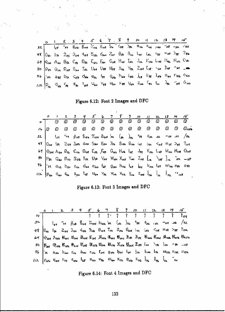
,C) 10. ir *~ 7. o t 12. 13 i

3z,. ff & $ /.ci. "lo 3 W ( '9 )Sff IM~ +14 a1 -3z c72. 11 273I 31,, 6. ,z 1. 7, w ;

Figure 6.12: Font 2 Images and DFO

4 . 3 ~ c 7 f 7 10 11I X. 13 1,Y /,I

32. Q~. ~ i.T 2 U !j~ %011c &261 f32q 1'5:L [ A \\ 1q I.- /-?

17 0% '32. 2,~ iiv c,,. 4c, . 6,2 7;,& 8Oiw & 9 :.%, I q k,0 <o =fl >Itb 0?O

P,1. Cb.l&, ,,,, S L aT U f, Vt,.q %k. . X 11Yq q Ii11%S If Ill -, - V

Figure 6.13: Font 3 Images and DFO

o 1 2.. 3 -7 4 7 2 10 1( 12-. 13 If~

9(. ';j. til, ttlto 1~il i3o r,3(, f104 ua*x 11IA to I i 7 hmq 17& lir,. i3,u ,37,

Figure 6.14: Font 4 Images and DFC

132

* -story.in, -a 64 character sentence.

9 command.com - the first 64 characters of an executable file.

,* xor7.cht - the-first 64 characters of a graphics file.

* parity8.fng - the first 64 characters of a numeric data file.

Only parity8.fng decomposed, to a cost of 220. The size of all these files increased,typically to around 90 bytes when, PKARC'ed. Apparently, there is no interestingcompression activity for files that are this small.

In order to allow us to run larger files, we considered each bit of a byte to be adifferent function. Now we can look at 512 byte files as 8 functions each on 9 variables.We ran several files like this.

* cin.asc, 537 bytes, a text file containing the first 512 characters of Chapter 1.

# hawaii.asc, 524 bytes, a text file containing the first paragraph of an exampledata text file from enableOA4 .

* data.asc, 519 bytes, a section of the numerical data from the FERD experiment.

* dbf.asc, 520 bytes, a section of the example data base file from enableOA.

* west.muz, 519 bytes, a section of a file of music data for Pianoman5 .

* auld.muz, 519 bytes, a section of a file of music data for Pianoman.

* mousea.ss, 516 bytes, a section from the first part of VGA image of a mouse.

* mouseb.ss, 516 bytes, a section from the middle of VGA image of a mouse.

* mousec.ss, 516 bytes, a section from the last part of VGA image of a mouse.

The results for each run are listed in Table 6.30 where the rows identified as 1, 2,etc. are the DFC for output bits 1, 2, etc. of the file labeling the appropriate column.The row labeled "Total" is the sum of the DFC's for all eight bits. The rows labeledPKARC and PKZIP are the compressed file size in bits. These results are summarizedin Table 6.31, where L is the length of an encoding of the decomposition.

We also generated some functions with trivial decompositions to see what PKARCand PKZIP would do with them.

e (file name: rand0l) A random string of ASCII O's and l's. The file had 514bytes. Bits 1-7 had zero DFC and bit 8 did not decompose. Therefore, DFC =512 or 12.5 percent, L = 646 or 15.8 percent, PKARC = 173 bytes or 33.7 per-cent, PKZIP = 244 bytes or 47.4 percent.

'1Trademark of Enable Software Inc.'Neil J. Rubenking, 1988.

133

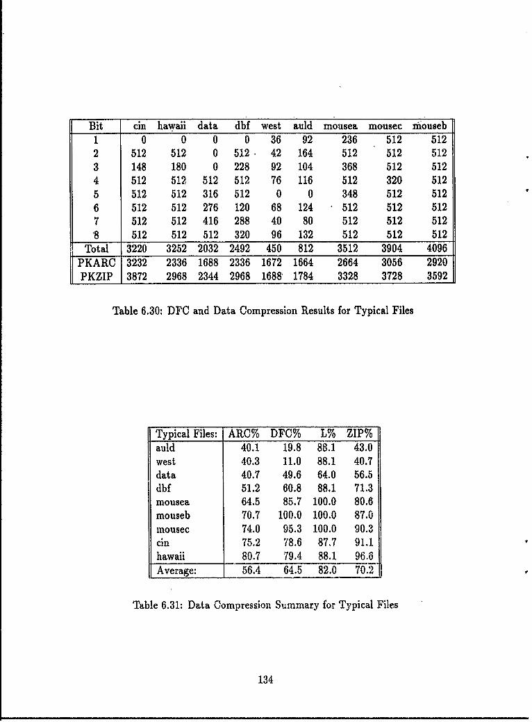
Bit cin hawaii data dbf west auld mousea mousec mouseb1 0 0 0 0 36 92 236 512 5122 512 512 0 512 42 164 512 512 5123 148 180 0 228 92 104 368 512 512

4 512 512 512 512 76 116 512 320 5125 512 512 316 512 0 0 348 512 5126 512 512 276 120 68 124 512 512 5127 512 512 416 288 40 80 512 512 512'8 512 512 512 320 96 132 512 512 512

Total 3220 3252 2032 2492 450 812 3512 3904 4096PKARC 3232 2336 1688 2336 1672 1664 2664 3056 2920PKZIP 3872 2968 2344 2968 1688 1784 3328 3728 3592

Table 6.30: DFC and Data Compression Results for Typical Files

Typical Files: ARC% DFC% L% ZIP%auld 40.1 19.8 88.1 43.0west 40.3 11.0 88.1 40.7data 40.7 49.6 64.0 56.5dbf 51.2 60.8 88.1 71.3mousea 64.5 85.7 100.0 80.6mouseb 70.7 100.0 100.0 87.0mousec 74.0 95.3 100.0 90.3cin 75.2 78.6 87.7 91.1hawaii 80.7 79.4 88.1 96.6Average: 56.4 64.5 82.0 70.2

Table 6.31: Data Compression Summary for Typical Files

134

Contrived files: ARC%: DFC%: L%: ZIP%:zeros 8.0 0.0 3.7 30.5spaces 8.7 6.8 27.8 47.3zeroone 16.7 0.0 3.7 33.7majgate 26.6 2.3 15.8 45.1randOl 33.7 12.5 15.8 47.4asciistr 94.4 0.0 3.7 85.5Average: 31.4 3.6 11.8 48.3All files Average: 48.4 40.1 58.3 63.1

Table 6.32: Data Compression Summary for Atypical Files

* (file name: majgate) A string of ASCII 0's and l's defining the majority gatefunction. The file had 514 bytes. Bits 1-7 had zero DFC and bit 8 decomposedto 96. Therefore, DFC = 96 or 2.3 percent, L = 646 or 15.8 percent, PKARC= 136 bytes or 26.6 percent, PKZIP = 232 bytes or 45.1 percent.

9 (file name: zeros) A string of ASCII O's. The file had 514 bytes. All 8 bits hadzero DFC. Therefore, DFC = 0 or 0 percent, L = 152 or 3.7 percent, PKARC= 42 bytes or 8.0 percent, PKZIP = 157 bytes or 30.5 percent.

* (file name: zeroone) A string of alternating ASCII 0's and l's. The file had516 bytes. All 8 bits had zero DFC. Therefore, DFC = 0 or 0 percent, L =152 or 3.7 percent, PKARC = 86 bytes or 16.7 percent, PKZIP = 174 bytes or33.7 percent.

* (file name: spaces) A file with two lines, each line has two ASCII l's separatedby 254 spaces. The file had 516 bytes. Six output bits had zero DFC, theother two had 4 minority elements so their cost is no more than 140. Therefore,DFC = 280 or 6.8 percent, L = 1140 or 27.8 percent, PKARC = 45 bytes or8.7 percent, PKZIP = 244 bytes or 47.3 percent.

* (file name: asciistr) A file with two lines, each line lists all ASCII characters inorder. The file had 517 bytes. All output bits had zero DFC. Therefore, DFC= 0 or 0 percent, L = 152 or 3.7 percent, PKARC = 488 bytes or 94.4 percent,PKZIP = 442 bytes or 85.5 percent.

These results are summarized in Table 6.32.The ARC, ZIP and AFD data are not directly comparable for several reasons.

The AFD representation is "random access" while the ARC and ZIP files must bedecompressed as a complete file. The ARC and ZIP compression routines run manytimes faster than AFD. DFC does not measure a complete representation (i.e. doesnot measure the interconnection complexity) and AFD does not optimize L. Also,for n = 9, as is the case for all these runs, L is bigger than 2" unless the function has

135

vacuous variables. That is, L includes a n2 [A] term and for no vacuous variables [A] >n. Therefore, L > n3 > 2" for n = 9. Therefore, we cannot expect decompositionto be a realistic data compression approach for small n. However, despite that, thedata compression performance for AFD (as measured by L) is in the same ball-parkas ARC and ZIP. That is, ARC had an average compression factor of 0.48 on allfiles, ZIP 0.63 and AFD 0.58. It is also interesting that there was a high degree ofcorrelation between pattern-ness as measured by DFC and the degree of compressionachieved by ARC and ZIP. For the typical files, the correlation coefficient betweenDFC and ARC was 0.87 and between DFC and ZIP it was 0.94. Remember thatthe ARC and ZIP compression programs were written by someone who had studiedthe common kinds of files and had recognized some patterns in these files that allowthem to be compressed. ARC and ZIP therefore look for specific kinds of patternsand those kinds of patterns were originally discovered by a person. AFD, on the otherhand, finds the patterns itself. The patterns it found in the files allowed compressionthat was comparable to that of the hand-crafted methods of ARC and ZIP. Thatthere is little pattern-ness beyond that considered by ARC and ZIP is evident in thehigh degree of correlation between DFC and the ARC and ZIP compression factorsfor typical files. That there exist some kinds of patterns that ARC and ZIP do notlook for is evident in the file assciistr where the DFC is 0 yet ARC and ZIP hadcompression factors between 0.85 and 0.95.

In summary, files were treated as functions and run on AFD. Not only does AFDfind patterns in yet another kind of function, it does so as well as programs hand-crafted for this class of patterns. The generality of AFD (and the lack of generality inthe hand-crafted programs) is indicated by an example where the compression factorfor AFD is less than 5 percent of that of the hand-crafted pattern finders.

6.3.7 Summary

It is our contention that DFC measures the essential pattern-ness that is important incomputing. We have the AFD algorithm that estimates DFC (never underestimatingthough). We took this algorithm and estimated the DFC of as many kinds of non-random functions as we could imagine. This involved about 850 decompositions.Table 6.33 is a summary of all the decompositions of the non-random functions. TheDFC column is an average when multiple runs are involved. Table 6.34 shows thatlarger n tends to have greater decomposability. With the current AFD algorithm,we are just able to decompose functions with sufficiently large n to have interestingpatterns; which makes these results all the more remarkable.

Recall that random functions do not decompose with high probability. In all 850runo there were only about 20 functions that did not decompose. As you look overTable 6.33 notice the correlation between DFC and the intuitive complexity of eachfunction. We believe that this is the most general quantitative measure of pattern-nessever proposed.

136

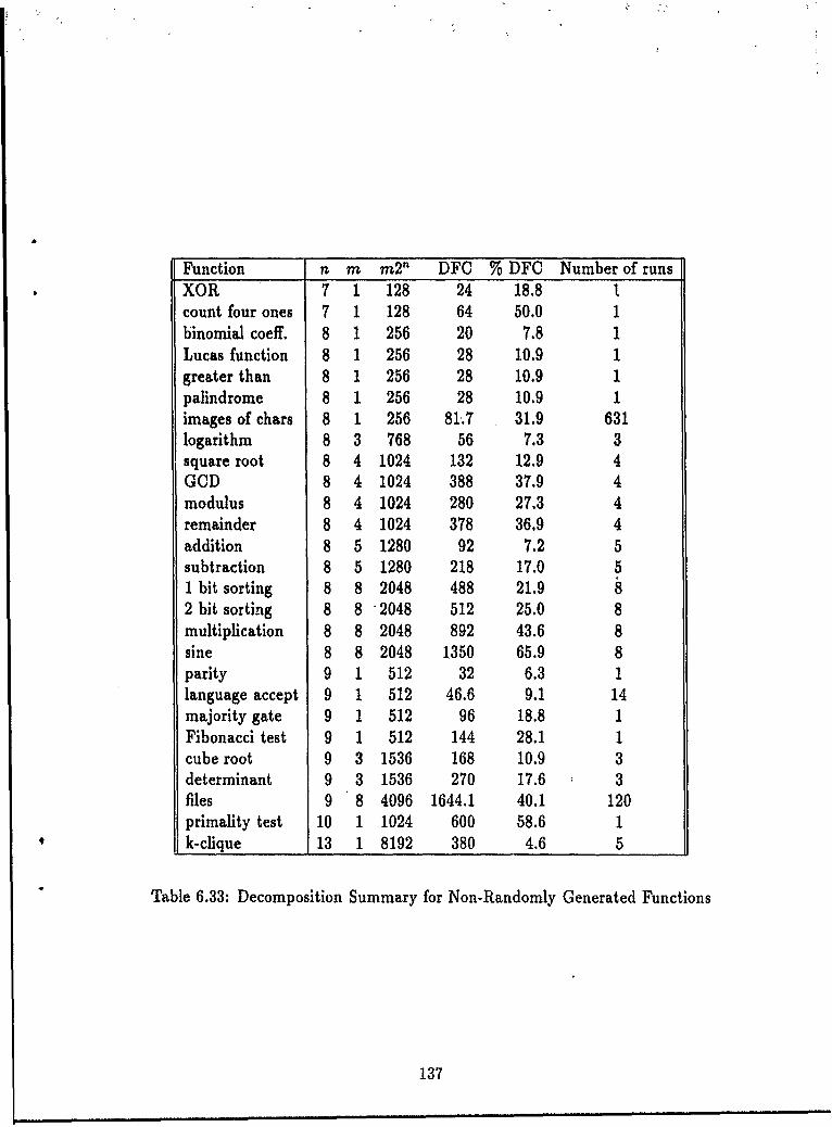
Function n m m2n DFO % DFC Number of runsXOR 7 1 128 24 18.8 tcount four ones 7 1 128 64 50.0 1binomial coeff. 8 1 256 20 '.8 1Lucas function 8 1 256 28 10.9 1greater than 8 1 256 28 10.9 1palindrome 8 1 256 28 10.9 1images of chars 8 1 256 81.7 31.9 631logarithm 8 3 768 56 7.3 3square root 8 4 1024 132 12.9 4GCD 8 4 1024 388 37.9 4modulus 8 4 1024 280 27.3 4remainder 8 4 1024 378 36.9 4addition 8 5 1280 92 7.2 5subtraction 8 5 1280 218 17.0 51 bit sorting 8 8 2048 488 21.9 §2 bit sorting 8 8 '2048 512 25.0 8multiplication 8 8 2048 892 43.6 8sine 8 8 2048 1350 65.9 8parity 9 1 512 32 6.3 1language accept 9 1 512 46.6 9.1 14majority gate 9 1 512 96 18.8 1Fibonacci test 9 1 512 144 28.1 1cube root 9 3 1536 168 10.9 3determinant 9 3 1536 270 17.6 3files 9 8 4096 1644.1 40.1 120primality test 10 1 1024 600 58.6 1k-clique 13 1 8192 380 4.6 5

Table 6.33: Decomposition Summary for Non-Randomly Generated Functions

137

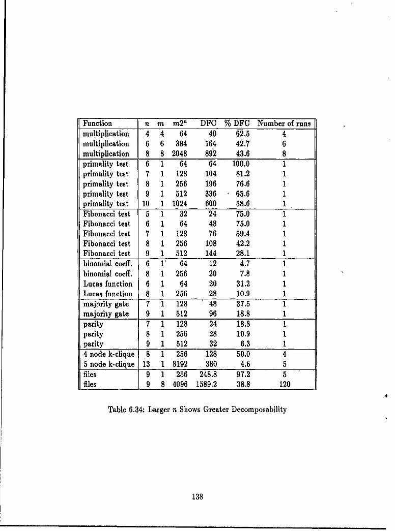
Function n m m2" DFC % DFC Number of runsmultiplication 4 4 64 40 62.5 4multiplication 6 6 384 164 42.7 6multiplication 8 8 2048 892 43.6 8primality test 6 1 64 64 100.0 1primality test 7 1 128 104 81.2 1primality test 8 1 256 196 76.6 1primality test 9 1 512 336 65.6 1primality test 10 1 1024 600 58.6 1Fibonacci test 5 1 32 24 75.0 1Fibonacci test 6 1 64 48 75.0 1Fibonacci test 7 1 128 76 59.4 1Fibonacci test 8 1 256 108 42.2 1Fibonacci test 9 1 512 144 28.1 1binomial coeff. 6 1' 64 12 4.7 1binomial coeff. 8 1 256 20 7.8 1Lucas function 6 1 64 20 31.2 1Lucas function 8 1 256 28 10.9 1majority gate 7 1 128 48 37.5 1majority gate 9 1 512 96 18.8 1parity 7 1 128 24 18.8 1parity 8 1 256 28 10.9 1parity 9 1 512 32 6.3 14 node k-clique 8 1 256 128 50.0 45 node k-clique 13 1 8192 380 4.6 5files 9 1 256 248.8 97.2 5files 9 8 4096 1589.2 38.8 120

Table 6.34: Larger n Shows Greater Decomposability

138

6.4 Patterns as Perceived by People

In this section we consider the relationship between complexity as measured by a func-tion decomposition algorithm and complexity as perceived by people when functionsare represented as two-dimensional images.

We have hypothesized that the DFC measure captures the essence of pattern-nessin general. DFC has established correlation with conventional measures such as timecomplexity, program length and circuit complexity. Since people are, in some sense,a computation system, we wonder: does this measure correlate with complexity asperceived by people? The AFD program provides the DFC measure of complexity. Toget human assessments of the complexity of these functions, we turned the functioninto something which can be easily perceived. There are a variety of possible ways ofdoing this. An image can be created from a function as discussed in Section 6.3.5. Asimilar method could be used to produce other experiences (e.g. sounds).

We generated a set of test functions, found the DFC complexity using the AFDprogram, found the complexity as perceived by people and assessed the relationshipbetween these two measures. Thomas Abraham reports the results of this study in[1]. In summary, this experiment found a correlation coefficient of 0.8 between DFCand pattern-ness as ranked by people.

6.4.1 Effect of the Order of Variables on the Pattern-nessof Images

At various points throughout the PT 1 study it has been useful to think of binaryfunctions as black and white images. This technique was used in the extrapolationexperiments, in the tests for DFC generality and in the pattern-ness/DFC correlationstudy just discussed.

In order to get an image from a binary function one must choose which variablesspecify rows and which specify columns. You must also decide the order among therow variables and among the column variables. This experiment is concerned with theeffect of the chosen grouping of variables on the appearance of the images. Table 6.35lists the images used in this experiment.

We used the Turbo Pascal character set (as in Section 6.3.5) as a source of func-tions. A program was used to draw a specified function with a variety of variablepermutations. Figures 6.15 through 6.18 show a sequence of images resulting fromthe program. Each figure has the character number, the font number, and the De-composed Function Cardinality (DFC) listed at the bottom. At the top left of thefigure is the image as drawn by the Turbo Pascal procedure outtextxy. At top rightis the drawing of the function that was generated by "getting pixels" from the leftimage. The top two images should always be the same. The order of the variablesfor the top row's images can arbitrarily be labeled as 1, 2, 3, 4 for the columns and 5,6, 7, 8 for the rows. From left to right, the second row of images are a permutationof these variables as in Table 6.36. Permutation 1 is a swapping of the high and low

139

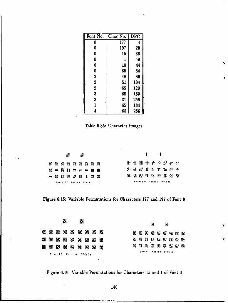
Font No. Char No. DFC0 177 40 197 200 15 360 1 400 10 440 65 642 48 802 51 1042 65 1203 65 1603 31 2561 65 1844 65 256

Table 6.35: Character Images

+I +

11. AEEi111C R 1-I.7 Fone O 0 rC 4 Ch ir I1 97 ront o OfC 20

Figure 6.15: Variable Permutations for Characters 177 and 197 of Font 0

Char: I ron, a o orc: 40

Char 15 Font:O OFC:36

Figure 6.16: Variable Permutations for Characters 15 and 1 of Font 0

140

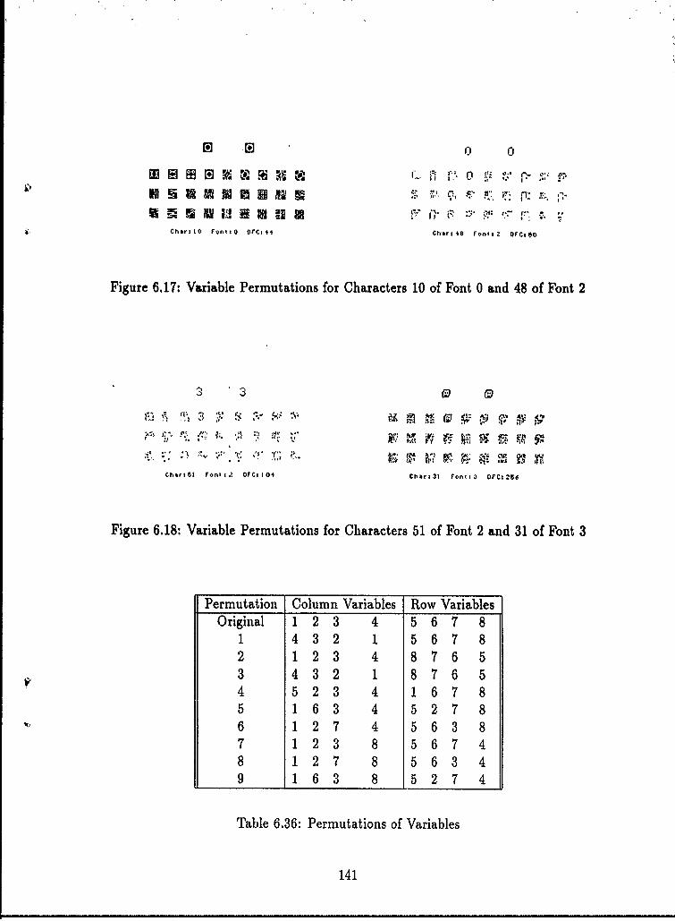
M. RE M. r.. Po o .*

0a a H I

Chart 10 FontO o t 1 I i Mlri4a rFot 12 OC 0O

Figure 6.17: Variable Permutations for Characters 10 of Font 0 and 48 of Font 2

3 3

Char ti Font . Drs 0 4 Chars 31 Font 1 3 orM 256

Figure 6.18: Variable Permutations for Characters 51 of Font 2 and 31 of Font 3

Permutation Column Variables Row VariablesOriginal 1 2 3 4 5 6 7 8

1 432 1 567 82 1 23 4 876 53 432 1 876 54 523 4 1 67 85 1 63 4 527 86 1 27 4 563 87 1 23 8 567 48 1 27 8 563 49 1 63 8 527 4

Table 6.36: Permutations of Variables

141

order bits of the column variables; 2 is a swapping of the high and low order bits ofthe row variables; 3 is a swapping of the high and low order bits of both the columnand row variables; 4 through 7 swap a column variable for a row variable; 8 swaps twoside-by-side column variables for two side-by-side row variables; 9 swaps every othercolumn variable for every other row variable. Note that all the font 0 characters haveat least two vacuous variables while none of the characters in the other fonts haveany vacuous variables.

This data shows that the apparent pattern-ness of a given function is highly de-pendent upon the variable permutation. For example, character 51 of font 2 withthe original combination of variables appears to be highly patterned while all of theimages resulting from a random permutations of the variables do not appear to bepatterned. This points out the risk in trying to "see" the patterns in a function byturning it into an image. There is at least one definite property, "connected-ness"that the original images have that is lost in the random permutations. Al but twoof the original images (i.e. all but characters 1 and 177 of font 0) are made up of nomore than 3 "islands." The randomly permuted images are made up of many moreof these islands. We argue that the "real" abstract pattern-ness of all the images ofa particular function is the same and that the difference in apparent pattern-ness isa result of our biological visual system.

6.5 Pattern-ness Relationships for Related Func-tions

When we defined the PT 1 problem (Section 3.4.9) we chose to only consider functionsdefined by tables. However, we eventually will consider functions defined in otherways. This raises the question, what does the pattern-ness of one function implyabout the pattern-ness of a related function? We are especially interested in thisquestion when one function is used to define a second function. For example, wemight be asked to compute y = f (x) where x = y'. What does knowing how tocompute x from y tell us about computing y from x? We hope to study this questionin depth in PT 2; however, we have some initial results that are described in thissection.

6.5.1 Functions and Their Complements

Perhaps the most trivial kind of relationship is when one function is simply thecomplement of a second function. If f(x) = g(not(x)) or not(g(x)) or not(g(not(x)))then f and g have the same DFC (except when f or g is a projection function).Not only is the DFC the same, so is the architecture of the decomposition (i.e. thealgorithm). Therefore, if we are asked to design an algorithm for f and f is definedfor us in the form of an algorithm for the complement of f then our job is very simple.

142

6.5.2 Functions and Their Inverses

This section is concerned with the relationship between the complexity of a functionand the complexity of that function's inverse6 and summarizes [30].

One motivation for studying this problem comes from the fact that many com-putational problems are originally specified in terms of the inverse of the functionwhich we want to realize. For example, there is the "classical inverse problem" ofcomputer vision. The transformation from a 3-D model of a space into a 2-D imageof that space from a particular perspective (Projective Geometry) is well understoodand of relatively low computational complexity. The computer vision problem is easyto specify using Projective Geometry. However, the objective in computer vision isto take a 2-D image and generate from that a 3-D model. Therefore, the problem isspecified using a function (Projective Geometry) which is the inverse of the functionthat we wish to realize on a computer. A second example is the situation where wewant to find an x with a particular given property y. Typically, the properties of x(say P(x)) are easy to compute and this is how the problem is specified. However,the inverse of P is needed to find x with a given input property y.

The question then arises; if a function (f) is of low computational complexity(which is generally the case when f is used in a problem specification) then shouldwe expect the inverse of f to have low computational complexity. In other words, ifa problem has a simple specification then does it necessarily have a simple computerrealization?

Our approach to studying this problem was to generate many functions and theirinverses and then compute their complexity. Since we are studying only true functions,we required the functions of this study to be bijections. That is, both the functionand its inverse are true functions.

This experiment was done with functions of the form:

f: 0,1I}, - {0,1}"'.

There are actually four functions going each way and the "cost" in the tables arethe sum of the DFC's of the four functions. We decomposed about 34,000 function -inverse pairs. Table 6.37 shows the relationship between functions with a given DFCand the average DFC of those function's inverses. Figure 6.19 shows the average DFCrelationship between functions and their inverses.

There are function-inverse pairs that have substantially different DFC's, e.g. 36versus 52 or 40 versus 56. However, they tended to be the same on average. In par-ticular, 19.9 percent of the functions had higher cost than their inverses, 20.2 percenthad lower cost and 59.9 percent had the same cost. The experimental correlationcoefficient between the DFC of a function and its inverse was 0.90. We observed fromthe detailed data that if one (or more) of the functions going one way was a projectionthen the inverse functions would also include the same number of projections. Thiswas also true of complements of projections.

6 This experiment was performed by John Lan~enderfer.

143

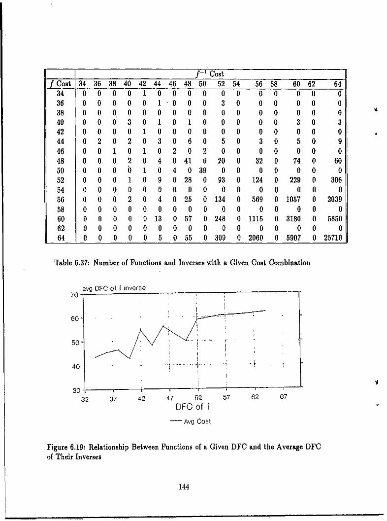
f- Costf Cost 34 36 38 40 42 44 46 48 50 52 54 56 58 60 62 64

34 0 0 0 0 1 0 0 0 0 0 0 0 0 0 0 036 0 0 0 0 0 1 0 0 0 3 0 0 0 0 0 038 0 0 0 0 0 0 0 0 0 0 0 0 0 0 0 040 0 0 0 3 0 1 0 1 0 0 0 0 0 3 0 342 0 0 0 0 1 0 0 0 0 0 0 0 0 0 0 044 0 2 0 2 0 3 0 6 0 5 0 3 0 5 0 946 0 0 1 0 1 0 2 0 2' 0 0 0 0 0 0 048 0 0 0 2 0 4 0 41 0 20 0 32 0 74 0 6050 0 0 0 b 1 0 4 0 39 0 0 0 0 0 0 052 0 0 0 1 0 9 0 28 0 93 0 124 0 229 0 30654 0 0 0 0 0 0 0 0 0 0 0 0 0 0 0 056 0 0 0 2 0 4 0 25 0 134 0 569 0 1057 0 203958 0 0 0 0 0 0 0 0 0 0 0 0 0 0 0 060 0 0 0 0 0 13 0 57 0 248 0 1115 0 3180 0 585062 0 0 0 0 0 0 0 0 0 0 0 0 0 0 0 064 0 0 0 0 0 5 0 55 0 309 0 2060 0 5907 0 25710

Table 6.37: Number of Functions and Inverses with a Given Cost Combination

avg DFC of f inverse70-

50 - ' ,

3032 37 42 47 52 57 62 67

DFO of I

Avg Cost

Figure 6.19: Relationship Between Functions of a Given DFC and the Average DFCof Their Inverses

144

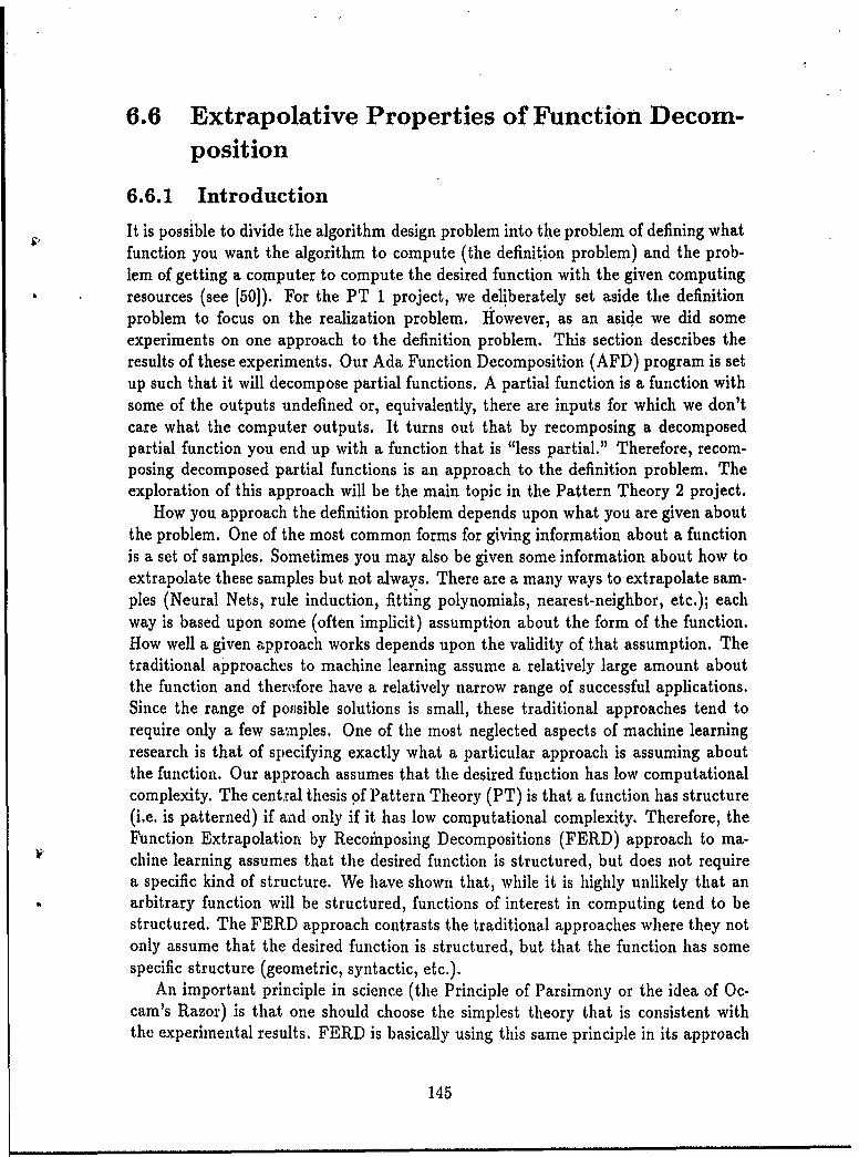
6.6 Extrapolative Properties of Function Decom-position

6.6.1 Introduction

It is possible to divide the algorithm design problem into the problem of defining whatfunction you want the algorithm to compute (the definition problem) and the prob-lem of getting a computer to compute the desired function with the given computingresources (see [50]). For the PT 1 project, we deliberately set aside the definitionproblem to focus on the realization problem. However, as an aside we did someexperiments on one approach to the definition problem. This section describes theresults of these experiments. Our Ada Function Decomposition (AFD) program is setup such that it will decompose partial functions. A partial function is a function withsome of the outputs undefined or, equivalently, there are inputs for which we don'tcare what the computer outputs. It turns out that by recomposing a decomposedpartial function you end up with a function that is "less partial." Therefore, recom-posing decomposed partial functions is an approach to the definition problem. Theexploration of this approach will be the main topic in the Pattern Theory 2 project.

How you approach the definition problem depends upon what you are given aboutthe problem. One of the most common forms for giving information about a functionis a set of samples. Sometimes you may also be given some information about how toextrapolate these samples but not always. There are a many ways to extrapolate sam-ples (Neural Nets, rule induction, fitting polynomials, nearest-neighbor, etc.); eachway is based upon some (often implicit) assumption about the form of the function.How well a given approach works depends upon the validity of that assumption. Thetraditional approaches to machine learning assume a relatively large amount aboutthe function and therefore have a relatively narrow range of successful applications.Since the range of poisible solutions is small, these traditional approaches tend torequire only a few samples. One of the most neglected aspects of machine learningresearch is that of specifying exactly what a particular approach is assuming aboutthe function. Our approach assumes that the desired function has low computationalcomplexity. The centxal thesis of Pattern Theory (PT) is that a function has structure(i.e. is patterned) if and only if it has low computational complexity. Therefore, theFunction Extrapolation by Recoinposing Decompositions (FERD) approach to ma-chine learning assumes that the desired function is structured, but does not requirea specific kind of structure. We have shown that, while it is highly unlikely that anarbitrary function will be structured, functions of interest in computing tend to bestructured. The FERD approach contrasts the traditional approaches where they notonly assume that the desired function is structured, but that the function has somespecific structure (geometric, syntactic, etc.).

An important principle in science (the Principle of Parsimony or the idea of Oc-cam's Razor) is that one should choose the simplest theory that is consistent withthe experimental results. FERD is basically using this same principle in its approach

145

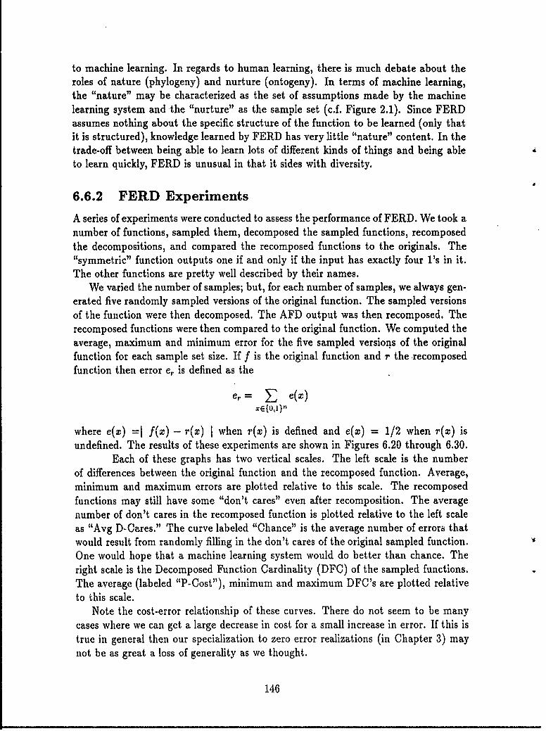
to machine learning. In regards to human learning, there is much debate about theroles of nature (phylogeny) and nurture (ontogeny). In terms of machine learning,the "nature" may be characterized as the set of assumptions made by the machinelearning system and the "nurture" as the sample set (c.f. Figure 2.1). Since FERDassumes nothing about the specific structure of the function to be learned (only thatit is structured), knowledge learned by FERD has very little "nature" content. In thetrade-off between being able to learn lots of different kinds of things and being ableto learn quickly, FERD is unusual in that it sides with diversity.

6.6.2 FERD Experiments

A series of experiments were conducted to assess the performance of FERD. We took anumber of functions, sampled them, decomposed the sampled functions, recomposedthe decompositions, and compared the recomposed functions to the originals. The"symmetric" function outputs one if and only if the input has exactly four l's in it.The other functions are pretty well described by their names.

We varied the number of samples; but, for each number of samples, we always gen-erated five randomly sampled versions of the original function. The sampled versionsof the function were then decomposed. The AFD output was then recomposed. Therecomposed functions were then compared to the original function. We computed theaverage, maximum and minimum error for the five sampled versions of the originalfunction for each sample set size. If f is the original function and r the recomposedfunction then error e, is defined as the

er= e(x)XE{O,1}n

where e(x) =1 f(x) - r(x) I when r(x) is defined and e(x) = 1/2 when r(x) isundefined. The results of these experiments are shown in Figures 6.20 through 6.30.

Each of these graphs has two vertical scales. The left scale is the numberof differences between the original function and the recomposed function. Average,minimum and maximum errors are plotted relative to this scale. The recomposedfunctions may still have some "don't cares" even after recomposition. The averagenumber of don't cares in the recomposed function is plotted relative to the left scaleas "Avg D-Cares." The curve labeled "Chance" is the average number of errors thatwould result from randomly filling in the don't cares of the original sampled function.One would hope that a machine learning system would do better than chance. Theright scale is the Decomposed Function Cardinality (DFC) of the sampled functions.The average (labeled "P-Cost"), minimum and maximum DFC's are plotted relativeto this scale.

Note the cost-error relationship of these curves. There do not seem to be manycases where we can get a large decrease in cost for a small increase in error. If this istrue in general then our specialization to zero error realizations (in Chapter 3) maynot be as great a loss of generality as we thought.

146

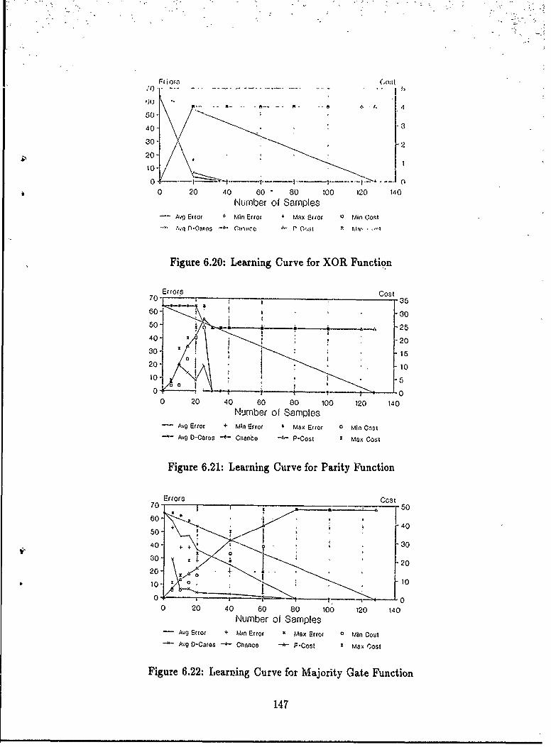
F-t i or, (,om 4

50.

40-' -3

220"

tII -- --100

0 20 40 60 80 100 120 140Number of Samples

-- Avg Error 4 Min Error Max Error U Min QoSI/,vk D-Caros -4- fl'r e A-- V CX . ..

Figure 6.20: Learning Curve for XOR Function

Errors Cost

60- - 30

50- -. 2

4 0 o - 2 0

20 , 10

10 1 1

050 . . 0


Avg Error + MIN Error Max Error Min Cost

Avg O-Caros -4- Chance - P-Cost Z Max Cost

Figure 6.21: Learning Curve for Parity Function

Errors Cost

60- ,+ - 4050- ,0

30 .2802, 0- z 0

'to 0 '10 :'


- Avg Error + Min Error 4 Max Error 0 Min Cot

--- Avg D-Caros -! Chance 4- F-Cost S Max Gosi

Figure 6.22: Learning Curve for Majority Gate Function

147

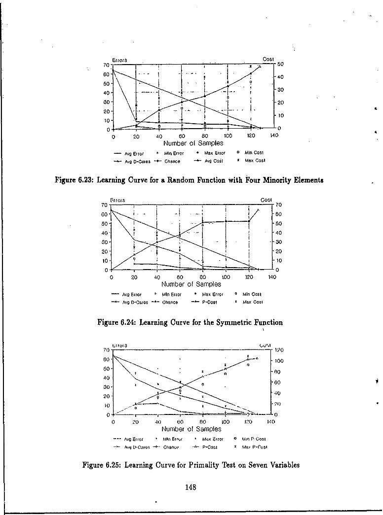
ErrorsCost

50 _0

601040

0 A0 40 6 8 0310 10

3- Av2ro0 ~nErr a ro mCs

205040

0 20 40 60 80 100 120 140

Number of Samples-Avg Error + in Error Max Error 0 Mi Cost

- Avg -Cars !h Chance Av PCol I Max Cost

~~~Figure 6.2 4: Learning Curve for th Symmetri FunctionWihPuMnotyEe ns

70 - 0

60 too50 05

40- 4

30-0 -60

20* 40

10~

0 --r0o 20 'to 60 80 too 120 140

Number of Samples-Avg Error Min Error 6 Max E~rror 0 Min tCos

SAvg L)'Caros 4O Can P-Cost X Max PCot

Figure 6.2: Learning Curve for r ty eo S eveticFncViable

1480

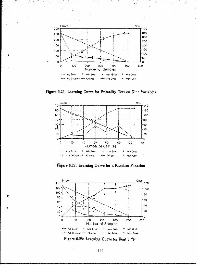
Cost

2001 200

250- -50

-0020 10 -023050050 O

0


- Avg Error + Minr Error * Max Error 0 Min Cost

~- Avg 0-Cares Chance -41- P-gCost zMax Cost

Figure 6.2 : Learning Curve for iat Rand om FunctVio le

Errors Cost10 -120

10-2

0- -0

20- 40

104-

0 "00 0 5 00 15 0 200 20 140

Number of Sampl'es- Avg Error + Min Error * Max Error 0 Min Cost

-- Avg -Cars -- Chance -AgCost Imax Cost

Figure 6.2: Learning Curve for Fanot Functio

140- 1 1 2 2

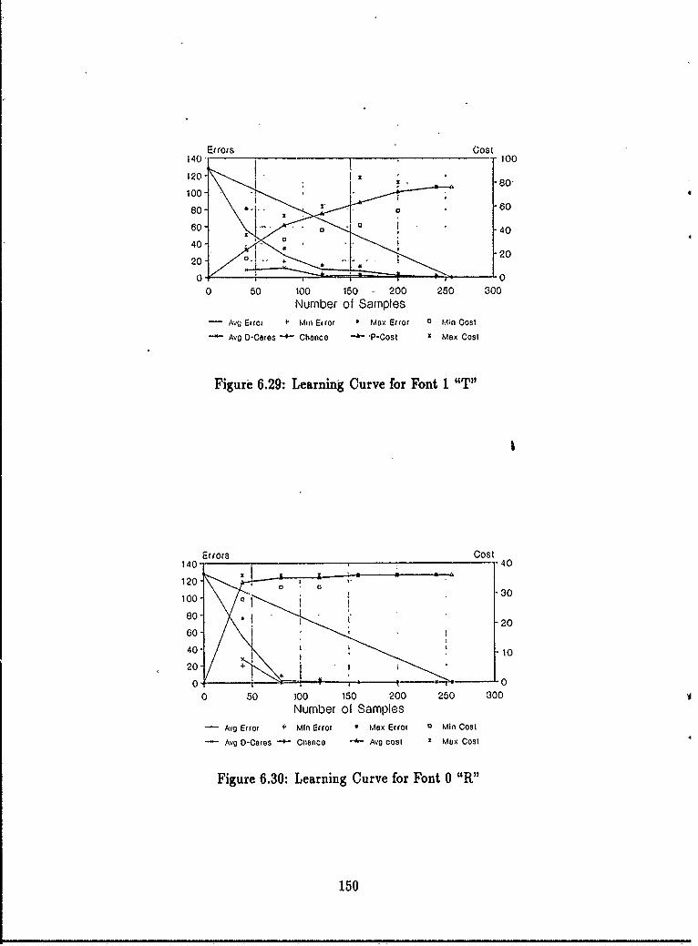
14-Errors cost10

-80.

1020

40-o

0 50 100 150 -200 250 300Number of Samples

- Avg Error Min Error max Error 0 Min Cost

Avg 0-Cares -- Chance -'P-Cost 11 Max Cost

Figure 6.29: Learning Curve for Font 1 "T"

Errors Cost140- 40

8030

-20

0 s0 100 150 200 250 300Number of Samples

-Avg Error +Min Error *Max Error 0Min Cost

-Avg 0-Cares -- Chance -- Avg cost max Cost

Figure 6.30: Learning Curve for Font 0 "'R"

150

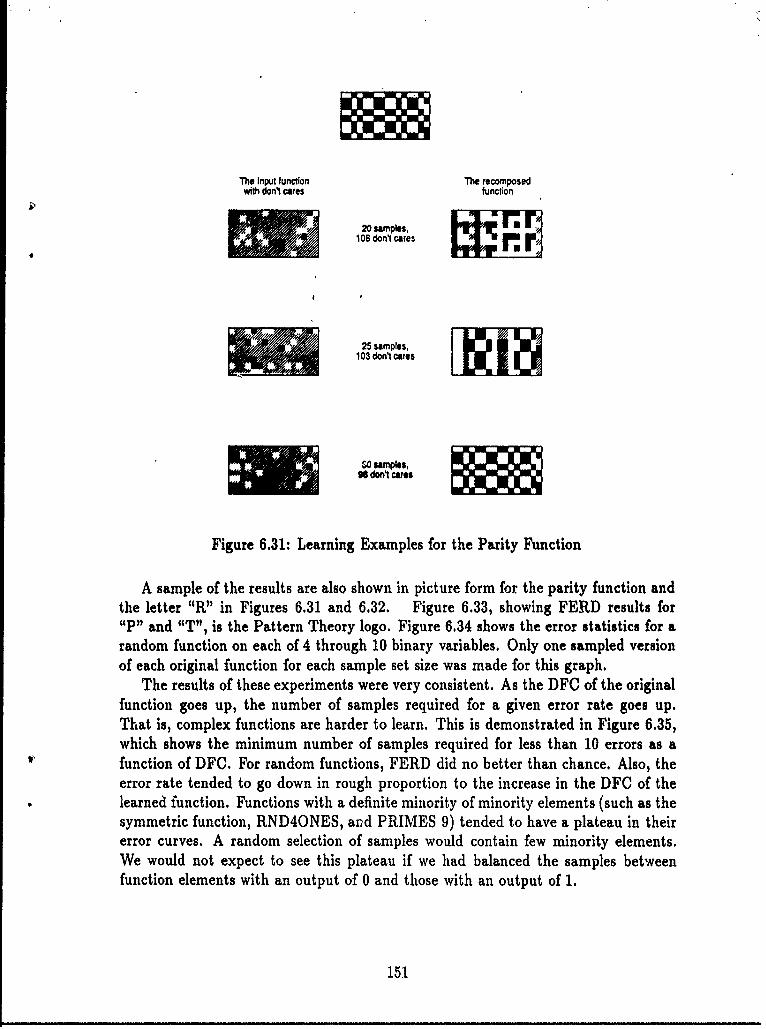
The Input function The recomposedwith don't cares function

20 samples,108 don't cares

103 don't cares

SO samples, ElEI98 don't cares

Figure 6.31: Learning Examples for the Parity Function

A sample of the results are also shown in picture form for the parity function andthe letter "R" in Figures 6.31 and 6.32. Figure 6.33, showing FERD results for"P" and "T", is the Pattern Theory logo. Figure 6.34 shows the error statistics for arandom function on each of 4 through 10 binary variables. Only one sampled versionof each original function for each sample set size was made for this graph.

The results of these experiments were very consistent. As the DFC of the originalfunction goes up, the number of samples required for a given error rate goes up.That is, complex functions are harder to learn. This is demonstrated in Figure 6.35,which shows the minimum number of samples required for less than 10 errors as afunction of DFC. For random functions, FERD did no better than chance. Also, theerror rate tended to go down in rough proportion to the increase in the DFC of thelearned function. Functions with a definite minority of minority elements (such as thesymmetric function, RND4ONES, and PRIMES 9) tended to have a plateau in theirerror curves. A random selection of samples would contain few minority elements.We would not expect to see this plateau if we had balanced the samples betweenfunction elements with an output of 0 and those with an output of 1.

151

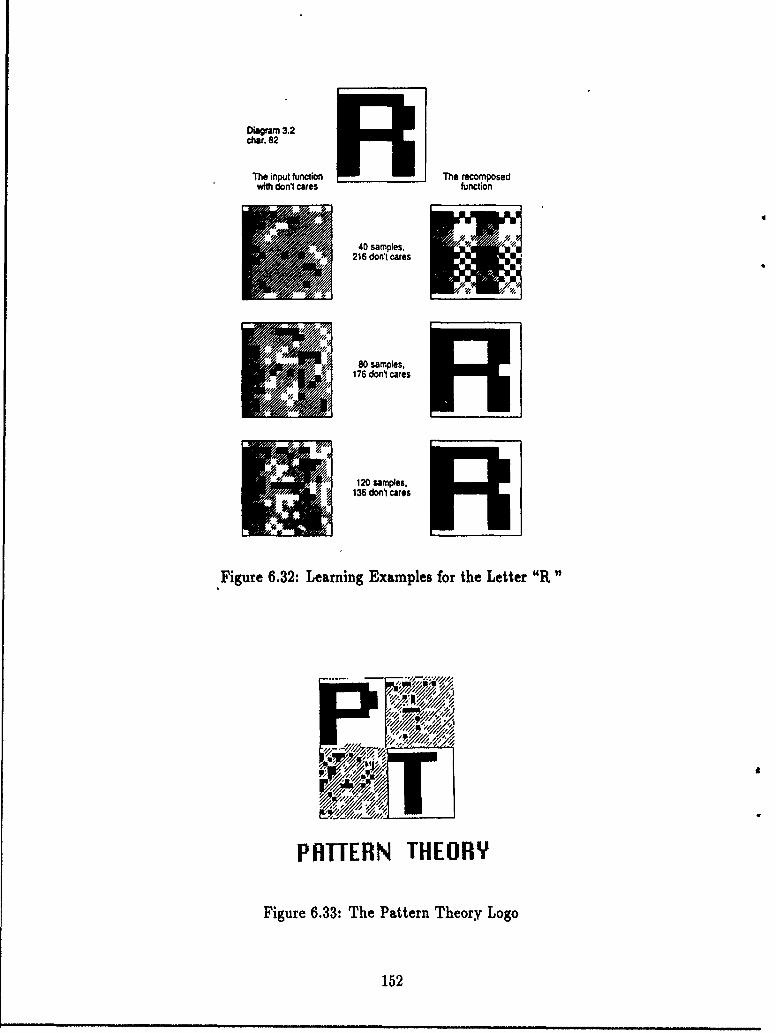
Diagram 3.2cha. 82

The input function I The recomposedwit don't cares function

Q 4 samples,. '

216 don't cares

80 sample,176 don't cares

A 120 samples.136 don't cares

Figure 6.32: Learning Examples for the Letter "R"

,~~4

PRTTERN THEORY

Figure 6.33: The Pattern Theory Logo

152

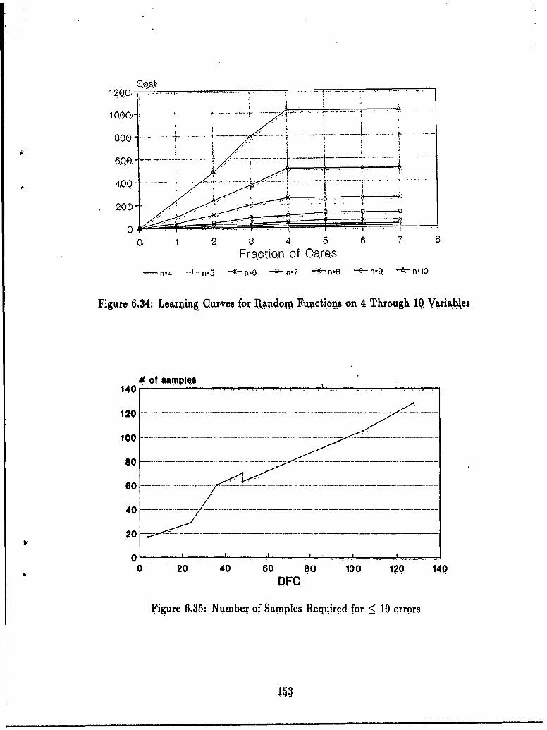
1000'

800t-.

400 --

200

0. 2 3 4 5 6 7 8Fraction of Oares

- n-4 --i-- -*n'- 6 -7 n±..8 --- n-9, 10

Figure 6.34: Learning Ourve for RkaudqM Fuctions on 4 Through 10. YVgiae

# of samlqo140 ..- -

120

20-

0 4

0 20 40 60 80 100 120 140DFC

Figu~re 6.35: Number of Samples Requ~ired for < 10 errors

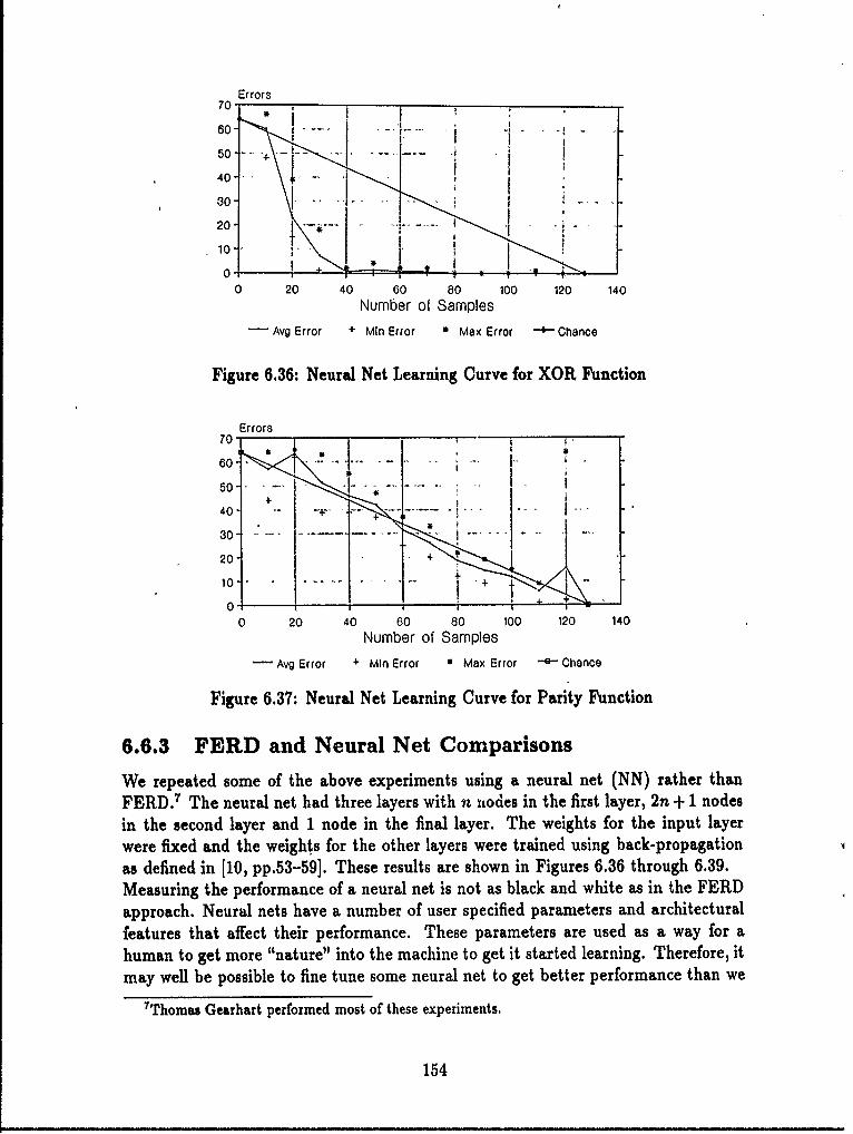
Errors70 - ,

60-. . .. . . . .--

50 '

30.20 1"

10 • i-


- Avg Error + Min Error 1 Max Error * Chance

Figure 6.36: Neural Net Learning Curve for XOR Function

Errors

60 . . . ... .

40 -. . .I. . .. .

30 -

10- t +


Avg Error + MIn Error • Max Error * Chance

Figure 6.37: Neural Net Learning Curve for Parity Function

6.6.3 FERD and Neural Net Comparisons

We repeated some of the above experiments using a neural net (NN) rather thanFERD.7 The neural net had three layers with n nodes in the first layer, 2n + 1 nodesin the second layer and 1 node in the final layer. The weights for the input layerwere fixed and the weights for the other layers were trained using back-propagationas defined in [10, pp.53-59]. These results are shown in Figures 6.36 through 6.39.Measuring the performance of a neural net is not as black and white as in the FERDapproach. Neural nets have a number of user specified parameters and architecturalfeatures that affect their performance. These parameters are used as a way for ahuman to get more "nature" into the machine to get it started learning. Therefore, itmay well be possible to fine tune some neural net to get better performance than we

TThomas Gearhart performed most of these experiments.

154

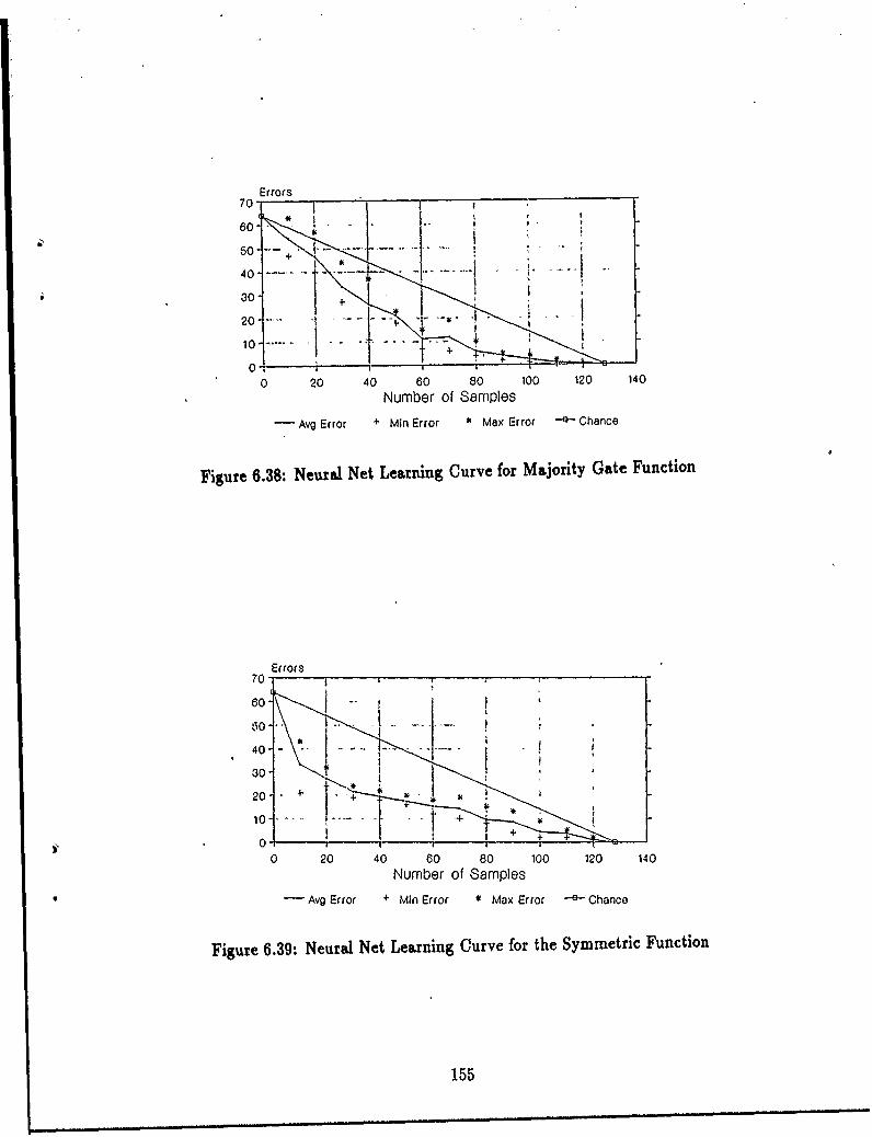
70 Errors

++

20 ,"

10. i7 i0..

0 20 40 60 8o 100 120 140

Number of Samples

Avg Error + Min Error • Max Error -- Chance

Figure 6.38: Neural Net Learning Curve for Majority Gate Function

Errors70

60

40 ,

30 "

20O

loi - 410-0 .1.

0 20 40 60 80 100 120 140

Number of Samples

- Avg Error + Min Error * Max Error - Chance

Figure 6.39: Neural Net Learning Curve for the Symmetric Function

155

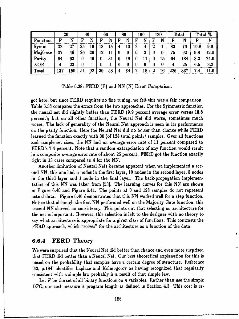
20 40 60 80 100 120 Total Total %Function F N F N F N F N F N F N" F N F NSymm 32 27 25 19 18 15 4 10 2 4 2 1 83 76 10.8 9.9MajGate 37 46 26 26 12 11 0 6 0 3 0 0 75 92 9.8 12.0Parity 64 63 0 46 0 31 0 18 0 11 0 15 64 184 8.3 24.0XOR 4 23 0 1 0 1 0 0 0 0 0 0 4 25 0.5 3.3Total 137 159 51 92 30 58 4 34 2 18 2 16 226 337 7.4 11.0

Table 6.38: FERD (F) and NN (N) Error Comparison

got here; but since FERD requires no fine tuning, we felt this was a fair comparison.Table 6.38 compares the errors from the two approaches. For the Symmetric functionthe neural net did slightly better than FERD (9.9 percent average error versus 10.8percent); but on all other functions, the Neural Net did worse, sometimes muchworse. The lack of generality of the Neural Net approach is seen in its performanceon the parity function. Here the Neural Net did no better than chance while FERDlearned the function exactly with 30 (of 128 total pointb) samples. Over all functionsand sample set sizes, the NN had an average error rate of 11 percent compared toFERD's 7.4 percent. Note that a random extrapolation of any function would resultin a composite average error rate of about 25 percent. FERD got the function exactlyright in 13 cases compared to 4 for the NN.

Another limitation of Neural Nets became apparent when we implemented a sec-ond NN, this one had n nodes in the first layer, 10 nodes in the second layer, 5 nodesin the third layer and 1 node in the final layer. The back-propagation implemen-tation of this NN was taken from [53]. The learning curves for this NN are shownin Figure 6.40 and Figure 6.41. The points at 0 and 128 samples do not representactual data. Figure 6.40 demonstrates that this NN worked well for a step function.Notice that although the first NN performed well on the Majority Gate function, thissecond NN showed no consistency. This points out that selecting an architecture forthe net is important. However, this selection is left to the designer with no theory tosay what architecture is appropriate for a given class of functions. This contrasts theFERD approach, which "solves" for the architecture as a function of the data.

6.6.4 FERD Theory

We were surprised that the Neural Net did better than chance and even more surprisedthat FERD did better than a Neural Net. Our best theoretical explanation for this isbased on the probability that samples have a certain degree of structure. Reference[33, p.194] identifies Laplace and Kolmogorov as having recognized that regularityconsistent with a simple law probably is a result of that simple law.

Let F be the set of all binary functions on n variables. Rather than use the simpleDFC, our cost measure is program length as defined in Section 4.3. This cost is es-

156

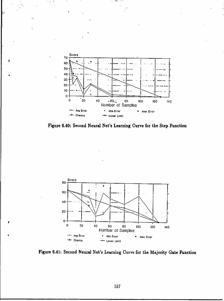
Errors

60 2 0 6o 0 2 4

G-- Cac ~ oe ii

115

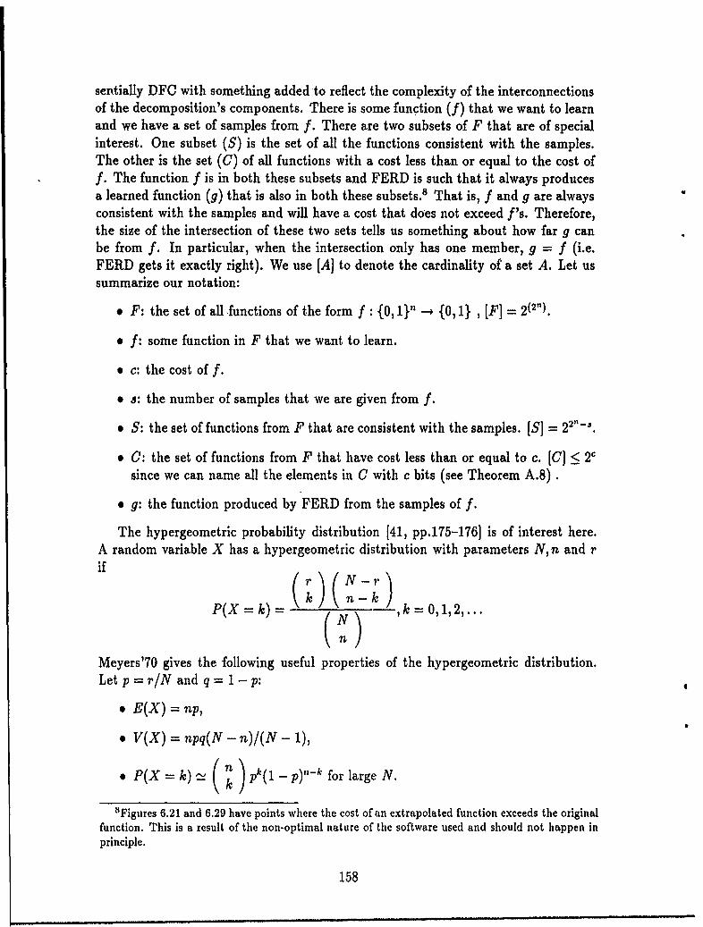
sentially DFC with something added to reflect the complexity of the interconnectionsof the decomposition's components. There is some function (f) that we want to learnand we have a set of samples from f. There are two subsets of F that are of specialinterest. One subset (S) is the set of all the functions consistent with the samples.The other is the set (C) of all functions with a cost less than or equal to the cost off. The function f is in both these subsets and FERD is such that it always producesa learned function (g) that is also in both these subsets.' That is, f and g are alwaysconsistent with the samples and will have a cost that does not exceed f's. Therefore,the size of the intersection of these two sets tells us something about how far g canbe from f. In particular, when the intersection only has one member, g = f (i.e.FERD gets it exactly right). We use [A] to denote the cardinality of a set A. Let ussummarize our notation:

* F: the set of all .functions of the form f: {0, 1}" - {0, 1} , [F] = 2(2n).

• f: some function in F that we want to learn.

* c: the cost of f.

* a: the number of samples that we are given from f.

e S: the set of functions from F that are consistent with the samples. [S] - 22"-s.

9 C: the set of functions from F that have cost less than or equal to c. [C] < 2c

since we can name all the elements in C with c bits (see Theorem A.8) .

9 g: the function produced by FERD from the samples of f.

The hypergeometric probability distribution [41, pp.175-176] is of interest here.A random variable X has a hypergeometric distribution with parameters N, n and rif ( XN -( r)

P(X = k) - ,k = O,1,2,...

Meyers'70 gives the following useful properties of the hypergeometric distribution.Let p =r/N and q = 1- p:

* E(X) = np,

* V(X) = npq(N - n)/(N - 1),

* P(X= k)- ( ) p)k(l -p)- for large N.

'Figures 6.21 and 6.29 have points where the cost of an extrapolated function exceeds the originalfunction. This is a result of the non-optimal nature of the software used and should not happen inprinciple.

158

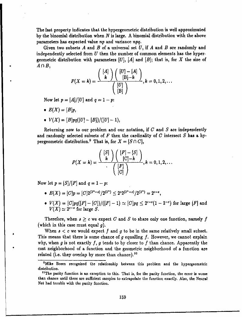
The last property indicates that the hypergeometric distribution is well approximatedby the binomial distribution when N is large. A binomial distribution with the aboveparameters has expected value np and variance npq.

Given two subsets A and B of a universal set U, if A and B are randomly andindependently selected from U then the number of common elements has the hyper-geometric distribution with parameters [U], [A] and [BI; that is, for X the size ofAnB,

P(X =k)= [B]- k ,= 0,1,2....

[B]Now let p = [A]/[U] and q 1 - p:

9 E(X) = [BJp,

* V(X) = [B]pq([Uj - [B])/([U] - 1),

Returning now to our problem and our notation, if C and S are independentlyand randomly selected subsets of F then the cardinality of C intersect S has a hy-pergeometric distribution.' That is, for X = [S n C],

IS (F] - (I

P(X=k)= [C)-k ,k = 0,1,2,...

Now let p = [S]/[F] and q = 1 - p:

* E(X) = [C]p =< 2[2 (n-,/2(2")= 2 ,-

* V(X) = [C]pq([F] - [C])/([FJ- 1) L [C]pq <_ 20-(1 - 2-') for large IF] andV(X) "' 2c- 3 for large S.

Therefore, when s > c we expect C and S to share only one function, namely f(which in this case must equal g).

When 8 < c we would expect f and g to be in the same relatively small subset.This means that there is some chance of g equalling f. However, we cannot explainwhy, when g is not exactly f, g tends to by closer to f than chance. Apparently thecost neighborhood of a function and the geometric neighborhood of a function arerelated (i.e. they overlap by more than chance)., 0

9Mike Breen recognized the relationship between this problem and the hypergeometricdistribution.

"The parity function is an exception to this. That is, for the parity function, the error is worsethan chance until there are sufficient samples to extrapolate the function exactly. Also, the NeuralNet had trouble with the parity function.

159

It seems that S is controlled by "geometric" distance while C is controlled bycost differences. What is the relationship between cost and geometric distance andhow does this relate to FERD? We first develop an upper bound on cost distanceas a function of geometric distance. Second, we draw some conclusions about the"topology" of the space of functions with respect to cost. Finally, we re-interpretsome earlier experimental results in a way that applies to this problem.

We can relate the geometric and cost distance between two functions by, in effect,using the computation of one function to compute the other. That is, we compute themore costly function by first computing the less costly function and then computingthe differences between the two functions. Define the geometric distance (d) betweentwo Boolean functions (f and g) on n variables as:

dg(f,g) = E f(x)-g(xI.xEX

This is equivalent to the number of points in which f and g differ. Define the costdistance (d,) between f and g as:

d,(f,g) =1 DFC(f) - DFC(g) 1,

where DFC(f) means the Decomposed Function Cardinality of f.

Theorem 6.9 If dg(f,g) < p then d,(f,g) < 4np.

Proof:Assume that dg(f,g) < p. Suppose f is the less expensive of the two functions. Wecan compute g by first computing f (with cost DFC(f)), computing the p minorityelements where f and g differ (with cost 4(n - 1) each, or a total of 4p(n - 1)) andthen summing f and the p minority elements together (with cost 4(k - 1), wherek = p + 1 is the number of variables to be summed, for a total cost of 4p). The DFCof g therefore must not be greater than the cost of the above computation, which isDFC(f) + 4p(n - 1) + 4p = DFC(f) + 4np. That is, DFC(g) <_ DFC(f) + 4np.0

Theorem 6.10 If dg(f,g) 2" - p then d,(f,g) < 4np + 2.

Proof:Note that d(f,g) >_ 2n - p implies dg(f, not(g)) <_ p, since if f and g disagree on allbut p points then f and not(g) agree on all but p points. We can compute not(g) asabove and then complement it with a cost of 2.0

If neither f nor g have cost < 2 then Theorem 6.10 has the slightly stronger formof Theorem 6.9: if dg(f,g) _ [f] - p then d,(f,g) < 4np, since the cost of a functionwith cost more than 2 is the same as its complement.

160

Theorem 6.9 tells us that functions within a local geometric neighborhood arealso within a local cost neighborhood. The converse of Theorem 6.9 is not true.Theorem 6.10 points out a certain kind of symmetry in the cost of functions as yougo from one point in the dq space of functions to its opposite point. The relationshipbetween dg and d. is analogous to the temperature distribution on the earth. Thetemperature everywhere inside this county is within a degree or two of the temperaturehere. However, when you consider the places that have temperatures about the sameas here, you might have to include places as far away as Europe or Asia. We think thatthe set of low cost functions form many small separated regions within the geometricspace of functions. We can think of the learning situation as one where S specifiesa fairly large connected geometric region and C specifies a bunch of small separategeometric regions. The geometric regions formed by S are "sub-spaces." For example,if F were 3-D then S might be a plane or a line. The intersection of S and C thenmight typically be just a sub-space of one of these small pockets of low cost. FERD,in effect, picks one of the lowest cost elements from S intersect C. Looking at thelearning curves, we see that as more and more samples are provided the minimumcost function has higher and higher cost. Also, when the cost of the minimum costfunction gets up to the cost of f, f is almost always the function FERD selects. Itseems the only way there would be more than one function of minimum cost is if thesub-space defined by S runs along a constant cost line (surface or whatever) ratherthan crossing it. Apparently the odds of that happening are not great.

The expected size of S intersect C is 2'- '. This result depends upon the assump-tion that S and C are randomly and independently selected from F. Let us examinethat assumption. Independence requires the distribution of functions with respect tocost within S to be the same as within F as a whole (as in P(C I S) = P(C)). Thefirst part of this section showed that within a small dg neighborhood independencedoes not hold. However, S is not small and its not really a neighborhood either. Weknow that all the functions in S are the same on the sample set so their dg is no morethan [f] - s. However, in real world learning applications, . is very small compared to[f]. That is, S is very large. For any function f, in S there exists a function f2, not isS, such that dg(f 1,f 2) = 1; that is, they differ only on some point in the sample set.That is, S is not what we would think of as a neighborhood. Therefore, Theorem 6.9does not pieclude independence between C and S for realistic situations.

There is some evidence suggesting that S and C are sufficien, 'y independent. Thisevidence comes from the minority element experiments (Sectie" 6.2.3). We studiedthe relationship between the number of minority elements in a function and thefunction's DFC. It appears that if the number of minority elements is greater thanabout 20 percent of the size of f then the cost distribution is random (at least theaverage DFC is about the same as a random distribution). The number of minorityelements in a function is the same as its d. from a constant function. Also, since theDFC of a constant function is zero, the DFC of a function is the same as its d, from aconstant function. Therefore, the DFC versus number-of-minority elements data canbe thought of as d. versus d, data relative to a constant function. If f is a constant

161

function and s is less than 60 percent of [f] then S looks pretty much like the set ofrandom functions with greater than 20 percent minority elements. Therefore, if a isless than 60 percent of [f], which it almost always will be, then the cost distributionon S is pretty much random. This means that S and C are reasonably independentunder the expected conditions. Intuitively, you" would think that you would haveto get further from a constant function than any other function before things lookrandom. Therefore, this conclusion that S has a random cost distribution relative toconstant functions is even more likely to be true for other functions.

6.6.5 Summary

In summary, FERD is an approach to function extrapolation that chooses the leastcomputationally complex function that is consistent with the samples. In effect,FERD chooses a function from the intersection of the set of low cost functions (C)and the set of functions consistent with the samples (S). Under an assumption ofindependence of C and S, the expected value of [C n S] is 2C-". We see some evidencethat this assumption may not be too bad in practice. Anecdotal comparisons of FERDand Neural Nets suggest that FERD has considerable potential as an extrapolationmethod. PT 2 will focus on FERD.

6.7 Summary

This chapter reports on the results of looking at the world from a Pattern Theoryperspective. We found that randomly generated functions have high DFO and thata very wide range of patterned functions (numeric, symbolic, string, graphic, imagesand files) have low DFC. There is high correlation between pattern-ness as measuredby DFC and as perceived by people. There is also high correlation between DFOand the compression factor for files. These results support the contention that DFCis a measure of the essential pattern-ness of a function. We also found the functiondecomposition has remarkably general extrapolative properties. This further supportsthe idea of a fundamental importance of decomposition.

162

Chapter 7

Conclusions andRecommendations

The theory of computing, as taught in most universities, fails the engineer in sev-eral ways. First, it makes much ado over something that is practically trivial, i.e.that there exists infinite functions that cannot be computed with finite machines(Appendix A). Second, the treatment of complexity results in a statement that ispractically not acceptable; i.e. that all finite functions have the same complexity (O(1)time complexity) (Section 4.4). Finally, and most importantly, the theory does notsupport design.

This report introduces a computing paradigm that we hope will support the en-gineering requirements. Note that .most of its elements (the decomposition condition[4], the relationship between combinational and time complexity [64], the theor: ofprogram length [12]) are known in the computing theory community, but lack thedeserved emphasis. If this report offers anything new to computing theory it is theidea of Decomposed Function Cardinality (DFC) as a general measure of essentialcomputational complexity. DFC correlates very well with the intuitive expectationsfor a general measure of pattern-ness. We ran the AFD program on a wide varietyof patterned functions. Recall that randomly generated functions do not decomposewith high probability. Therefore, it is quite remarkable that of the roughly 850 func-tions that we did not generate randomly, only about 20 did not decompose. We feelthat the generality of DFC as a measure of pattern-ness has been well demonstrated.

We can also start to see the potential for practical benefits from Pattern Theory.We have been working with what might be called "toy" problems (i.e. binary functionson no more than 10 or so variables). However, we believe that we should expect to beable to do algorithm design on toy problems before more general problems. Note thatthis is opposite from the approach taken in most machine learning paradigms. Thecommon view in machine learning is that we solve the easy problems by hand andwhen we get to problems that we cannot solve by hand such as the character recogni-tion (cannot solve the definition problem) or the traveling salesman problem (cannotsolve the realization problem) then we try to get a machine to solve it. We think thatwe should be able to machine learn (or machine design algorithms for) easy problems

163

long before we can machine learn the hard ones. Each time the AFD program foundthat a function had a low DFCf (which it did some 830 times), it also found an al-gorithm for that function. Therefore, although we were limited to toy problems, wehave demonstrated machine designed algorithms in a very general setting. From amachine learning perspective, FERD performed as well as a Neural Net on functionswell suited to Neural Nets and considerably outperformed the Neural Net on otherfunctions. Also, unlike most traditional machine learning paradigms, we can say ex-actly what property a function must have to be amenable to FERD extrapolation.That property is low computational complexity in the sense of DFC. Recall that DFCis a strikingly general sense of complexity and we begin to appreciate the significanceof FERD. Similarly, from a data compression perspective, function decompositionperformed comparably to hand-crafted compression algorithms on typical files andconsiderably outperformed them on atypical files. Therefore, we feel that PatternTheory represents a solid foundation for an engineering theory of computing.

The results of PT 1 clearly support the need for further exploration and develop-ment of Pattern Theory. Although PT 1 dealt with toy problems, we went from ageneral statement of the real problems to the PT 1 problem in a series of deliberatepartitions and simplifying assumptions. Therefore, our recommendations for futuredevelopments of Pattern Theory are simply to revisit each decision in defining thePT 1 problem and consider the implications of not making that decision.

164

Chapter 8

Summary

Algorithm technologies are very important to the Avionics Directorate because theyoffer a cost-effective means to realize adaptive and fault tolerant avionics capabilities.There is an un-met need for a theory of algorithm design. We only have to considerthe power of Estimation Theory or Control Theory to realize the importance of anengineering theory. This report proposes and discusses "Pattern Theory" as a basisfor an engineering theory of algorithm design.

Pattern Theory (PT) begins with a very general statement of the algorithm designproblem. This general problem covers virtually every other discipline that results ina computational system, including Neural Networks (NN) and model-based vision.Deliberate specializations to this general problem are made to arrive at the problemtreated in this report (the PT 1 problem). It is important (and unusual) to stateup-front how a specialized approach relates to the general problem.

The problem of finding a pattern in a function is the essence of algorithm design.The key to PT is its measure of pattern-ness: Decomposed Function Cardinality(DFC). The thesis is that low DFC indicates pattern-ness. This measure is uniquelygeneral in reflecting the low complexity that is associated with patterns. The proper-ties of DFC are defined and developed with mathematical rigor. The principal resultof PT 1 is a demonstration of the generality with which 1)FC measures pattern-ness.

The generality of DFC is suppcrted theoretically by 57 proven theorems. DFChas the property that if a function is computationally non-complex relative to timecomplexity or circuit complexity then it is necessarily non-complex with respect toDFC, while the converse is not necessarily true. The previous statement is not truerelative to program length since one can always assign an arbitrarily short programto any function. However, DFC has the property that its average is no more thana single bit greater than the average program length and, when decompositions areencoded as programs, the program length caanot be large without DFC also beinglarge. By rigorously relating DFC to time complexity, program length and circuitcomplexity it can be assured that the class of patterns defined by DFO includes theclasses of patterns that would be defined by these conventional measures. In doingthis, new results were also developed in the theory of program length (Appendix A).

PT 1 explored function decomposition algorithms as a means to find DFO pat-

165

terns. We developed a general test (the Basic Decomposition Condition), based onDFC, for whether or not a function will decompose for a given partition of its v4ri-ables. This test was then used in algorithms (collectively known as the Ada FunctionDecomposition (AFD) algorithms) with a variety of heuristics for limiting the depthof the search through iterative decompositions. AFD produces a decomposition (i.e.an algorithm in combinational form) and the DFC of a function. We did not findthe hoped for threshold where additional searching had no payoff. However, we didfind that the most restrictive search method came very close to performing as well asthe least restrictive search method, despite the several orders of magnitude greaterrun-time of the less restricted search. There was especially little benefit in the largersearch when the function being decomposed was highly patterned.

The generality of DFC was also supported experimentally. Over 800 non-randomlygenerated functions were tested including many kinds of functions (numeric, symbolic,string based, graph based, images and files). Roughly 98 percent of the non-randomlygenerated functions had low DFC (versus less than 1 perent for random functions).The 2 percent that did not decompose were the more complex of the non-randomlygenerated functions rather than some class of low complexity that AFD could notdeal with. It is important to note that when AFD says the DFC is low, which it didsome 800 times, it also provides an algorithm. AFD found the classical algorithmsfor a number of functions.

Some applications demonstrate the importance of DFC's generality. The correla-tion coefficient between DFC and a ranking of patterns by people was 0.8. In a datacompression application on typical files, the correlation coefficient between DFC andthe compression factor of two commercial data compression programs was about 0.9.However, on an atypical file, AFD had the much better compression factor of 0.04versus 0.86 and 0.94 for the commercial programs. In a machine learning applica-tion, AFD did as well as a NN on problems well suited to NN's. However, on anotherproblem, AFD learned a 128 point function from 30 samples whereas the NN requiredall 128 points. These applications demonstrate that traditional paradigms look for aparticular kind of pattern; when they find that pattern they, do well and when theydon't they do poorly. PT is unique in that it does not look for a particularkind of pattern, it looks for patterns in general.

PT is a pervasive technology and, at maturity, may revolutionize the approach tomany computational problems. Potential areas for early application of PT have beenidentified, such as algorithm development for Non-Cooperative Target Identification.PT has also shown promise in machine learning and data compression problems. Al-though PT 1 has laid the foundation and even identified potential early applications,there are many unsolved problems. PT 2 will begin to address the issues that limitthe application of decomposition to small problems.

166

Appendix A

Program Length and theCombinatorial Implications forComputing

A.1 Mathematical Preliminaries

A.1.1 Basic Definitions

A partial function f : X -+ Y is a set of ordered pairs from X x Y, where thereis at most one y E Y associated by f with any x E X. That is, (x, y) E f and(X,y') E f implies that y = y'. A total function is a partial function with theadditional property that f is defined on all of X. That is, for all x E X, there exists ay E Y such that (X,y) E f. We will also use the word "mapping" for a function. Theset X is called the domain of f. The set Y is called the codomain of f. The firstelement of all the pairs in f form a set called the base (this is not standard). Thebase of f is a subset of the domain of f. If f is total then the base of f equals thedomain of f. The second element of all the pairs of f form a set called the range.The range is a subset of the codomain. The image of an element x in the domainof f is the corresponding element y = f(x) in the range of f. When the range of amapping equals the codomain "of the mapping, the mapping is said to be surjectiveor "onto." Number theoretic functions are functions of the form f : N" -4 N,where N is the set of natural numbers.

The cardinality of a set A, denoted [A], is the number of elements in the set A ifA is a finite set. The cardinality of an infinite set is determined by which standard setit corresponds to in a one-to-one manner. The cardinals associated with infinite setsare called transfinite cardinals. Since a function f is also a set, [f] is well-definedand indicates the size of a function. Let c indicate the cardinality of the continuum(i.e. the real numbers) and Ro indicate the cardinality of a countably infinite set.We know that n ° equals c for any finite n greater than one [20, p.155 Equation 2].In general, a finite number to the power of a transfinite cardinal is the next larger

167

cardinal. We have a particular interest in the cardinality of sets involving the Naturalnumbers (N). All elements of N are finite. However, N is unbounded. That is, theredoes not exists a b E N such that n < b for all n E N. Therefore, N has cardinalityR, and a function with domain N, also has cardinality R. . The set of all possiblefunctions with domain N has cardinality c [59, p.12]. The relationship "<" can beinterpreted in a natural way on N and on transfinite numbers; i.e. n < R" < c for alln E N. That is, the elements of N have their usual order, the transfinite cardinalshave their usual order and all transfinite cardinals are greater than all finite cardinals.The relationship "=" also has a natural interpretation, so "<" can be used as well.

Let E be a set of symbols, not necessarily of finite cardinality. Let Q be N ora subset of N of the form {n E N I n < T} for some T E N. A string on E is amapping from Q into F for some Q. Define E* as the set of all possible strings on E.For x, a string in F*, we denote the length of x by s(x). We have not adopted thetraditional finite limitation on [B] and s(x). A language over E is a subset of E*

Let X 1, X2,... , X,, be arbitrary sets. An element of a product of sets (e.g. X, xX 2 x ... x Xn) is a vector. A vector is also a string with alphabet E = X, U X2 U... U Xn. Therefore, we designate the length of a vector s(x) as its length as a string.For a vector in X, x X 2 x ... x X, , s(x) = n.

A.1.2 CombinatoricsLet us review some basic combinatorics. We are especially interested in the cardinalityof the set of all vectors of a given length, the set of all strings no longer than a givenlength, and the set of all functions on a given domain. The following theorem givesthe cardinality of a set of vectors.

Theorem A.1 If V is the set of all vectors of length s(v) = n, that is V =

then there are [rja(v) vectors in V, i.e. (V] =-

Proof:There can be any one of [E] symbols in the first position. Then for each symbol inthe first position, there can be any one of [E] symbols in the second position. Thus,the number of combinations for a two-dimensional vector is [E][E] = [] 2. Similarly,for each combination of the first two symbols there can be any one of [E] symbols inthe third position. Thus, the number of combinations for a three-dimensional vectoris [E]2[] = [E]3. This argument can be continued to find that there are [E]' (' ) com-binations of symbols in an s(v)-dimensional vector.0

We now develop the cardinality of a set of strings on an alphabet E of [E] letters.

Theorem A.2 If L is the set of strings on E whose lengths are less than or equal to

some threshold s(l') then L] = -IEJ-1

168

Proof:If L is a subset of E*. Let I' be a string in L of the maximum allowed length. Thereare strings of length 0,1, 2,..., s(l'). For each string of length i there are [EJ] differentstrings (as with vectors). Therefore, there are a total of

8(1')

i=0

strings in L. Thus,

[ 8(' =_ ([8 ] - ) 1 ,)(o [) s(')+ [Eli ] _ ()[(=o - 1 = [J]-1

i=Op

'1i + [_]d(1+i []O + = ,[ F]' ¢p')+l. 1

The expression for the number of vectors is simpler than the expression for thenumber of strings, yet there is not much difference between the two.

Theorem A.3 For finite s(l') and s(l') = s(v), we have [V] < [L] < 2[V].

Proof:The first inequality follows from V being a proper subset of L. The second inequalitycan be developed as follows:

,+> []8()+1 _1 = [E]][J8() - 1 > 2[E]'(") - 1,

assuming [E] > 2. Thus,

[E]1 + 1 > 2[]1(") - 1,[]]) + 1 - 2[]1) >-I2]1(!+ 1 - 2[8 1( ') > [~]81')+1 - 1,

2[F]1(*)([8 ] - 1) > []s(V)+1 _ 12[]s4v) > (]],e+ )(1l )

Finally, since[IV] = []()= ](")

and

we have 2[V] > [L].0

169

Also, for transfinite s(t'), we have [L] = [V]; i.e. the addition, subtraction ormultiplication of a finite number with a transfinite cardinal yields the same transfinitecardinal. Therefore, for finite or transfinite s(l'), [L] and [V] are very similar. Let Fbe the set of all total functions of the form f : X - Y, where X and Y are arbitrarysets. A set of strings satisfies the prefix condition if no string in the set containsanother string from the set as its first letters.

Theorem A.4 The largest number of different strings of length < I and satisfyjingthe prefiz condition is the number of vectors of length 1.

Proof:Any string of length < I eliminates all longer strings with that beginning from the setof strings satisfying the prefix condition. There is always more than one string elimi-nated by a string of length < 1. A string of length I only eliminates itself. Therefore,the largest set of strings satisfying the prefix condition is the set of stings of lengthexactly 1.0

The following theorem gives the cardinality of a function.

Theorem A.5 If F is the set of all total functions of the form f : X -+ Y then[F]- [y-I'l.

Proof:Each function f E F can be thought of as a vector made up of the sequence of imagesunder f for all x E X. Thus, the cardinality of F is the cardinality of a set of vectorsof length [X] over the symbol set Y.0

We might have assumed that F is the set of all partial (rather than total) functionson a given domain. However, we can model any partial function g : X --* Y with atotal function f : X -4 (Y U {J'}), where y is some symbol not in Y. That is, letf(x) = g(xz) for any x in the base of g and let f(m) = y' for all other x's. Therefore,the set of all partial functions into Y has a one-to-one correspondence with the set ofall total functions into Y U {y'}. The number of partial functions into Y equals thenumber of total functions into Y U {y'}. The number of total functions into Y U {y'}is ([Y] + 1)tX1. The number of partial functions into Y is then ([Y] + 1)(Mi. Therefore,whether we use F as the set of all total functions or as the set of all partial functions,there is little difference in the essential combinatorics.

170

A.2 Program Length Constraints for Computa-tion

A.2.1 Introduction

In most texts on Computability Theory you will find a statement such as: there existnumber theoretic functions (i.e. functions on finite numbers) which cannot be com-puted with any finite program. The proof of this statement depends only upon somecombinatorial arguments. While this is clearly a most impressive consequence of thesecombinatorial considerations, the consequences are much broader than indicated bythat one statement. The objective of this appendix is to recognize and precisely statethe general computing limitations implied by combinatorial considerations. As com-pared with the traditional statement of noncomputability, the following statementsare stronger and more general, yet equally easy to derive.

Now it is reasonable to ask whether or not there exists a machine for a given Pand F. We kno.w from above that, regardless of the particular association desiredbetween P and F, these simple combinatorial constraints must be satisfied. If theyare not satisfied then we say that no machine exists which can be programmed fromP to compute any element of F. In particular, if we consider P = E, then [P] is Ro.If we also consider F to be the set of all functions on the set of all finite strings then,although s(x) is finite, [X] (or [f]) is K and [F] is c. Therefore, [P] is not greaterthan or equal to [F] and, consequently, there does not exist a machine which can beprogrammed from P to compute any element of F. This is the traditional statementof noncomputability.

We feel that the generalized developments of this appendix allow a more intuitiveintroduction to computability as well as the more general implications of programlength constraints. That is, first develop the max-min program length constraints.These constraints are intuitive and easy to develop from basic combinatorial con-siderations. With an understanding of these constraints, we can easily derive thetraditional noncomputability result as well as many other more general or strongerresults. The existence of noncomputable functions is uncoupled from the traditionalsources of confusion such as the relationship between transfinite cardinals and the rich(but irrelevant) structure of Turing machines and number theoretic functions. There-fore, although this alternative introduction to noncomputability is more general andstronger, it can also be more intuitive. We can then develop average-minimum pro-gram length constraints by applying Information Theoretic concepts to this paradigm.There are several practically important applications of these program length con-straints.

171

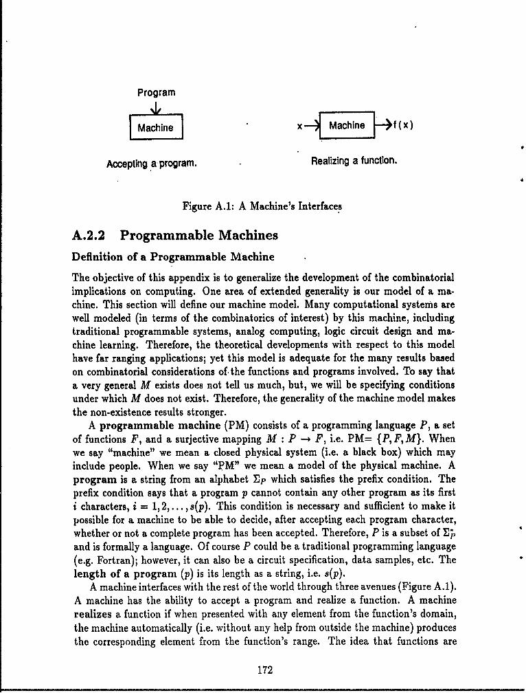
Program

Machine x Machine f(x)

Accepting a program. Realizing a function.

Figure A.1: A Machine's Interfaces

A.2.2 Programmable Machines

Definition of a Programmable Machine

The objective of this appendix is to generalize the development of the combinatorialimplications on computing. One area of extended generality is our model of a ma-chine. This section will define our machine model. Many computational systems arewell modeled (in terms of the combinatorics of interest) by this machine, includingtraditional programmable systems, analog computing, logic circuit design and ma-chine learning. Therefore, the theoretical developments with respect to this modelhave far ranging applications; yet this model is adequate for the many results basedon combinatorial considerations of. the functions and programs involved. To say thata very general M exists does not tell us much, but, we will be specifying conditionsunder which M does not exist. Therefore, the generality of the machine model makesthe non-existence results stronger.

A programmable machine (PM) consists of a programming language P, a setof functions F, and a surjective mapping M : P -- F, i.e. PM= {P, F, M}. Whenwe say "machine" we mean a closed physical system (i.e. a black box) which mayinclude people. When we say "PM" we mean a model of the physical machine. Aprogram is a string from an alphabet Ep which satisfies the prefix condition. Theprefix condition says that a program p cannot contain any other program as its firsti characters, i = 1,2,... ,s(p). This condition is necessary and sufficient to make itpossible for a machine to be able to decide, after accepting each program character,whether or not a complete program has been accepted. Therefore, P is a subset of E;,and is formally a language. Of course P could be a traditional programming language(e.g. Fortran); however, it can also be a circuit specification, data samples, etc. Thelength of a program (p) is its length as a string, i.e. s(p).

A machine interfaces with the rest of the world through three avenues (Figure A.1).A machine has the ability to accept a program and realize a function. A machinerealizes a function if when presented with any element from the function's domain,the machine automatically (i.e. without any help from outside the machine) producesthe corresponding element from the function's range. The idea that functions are

172

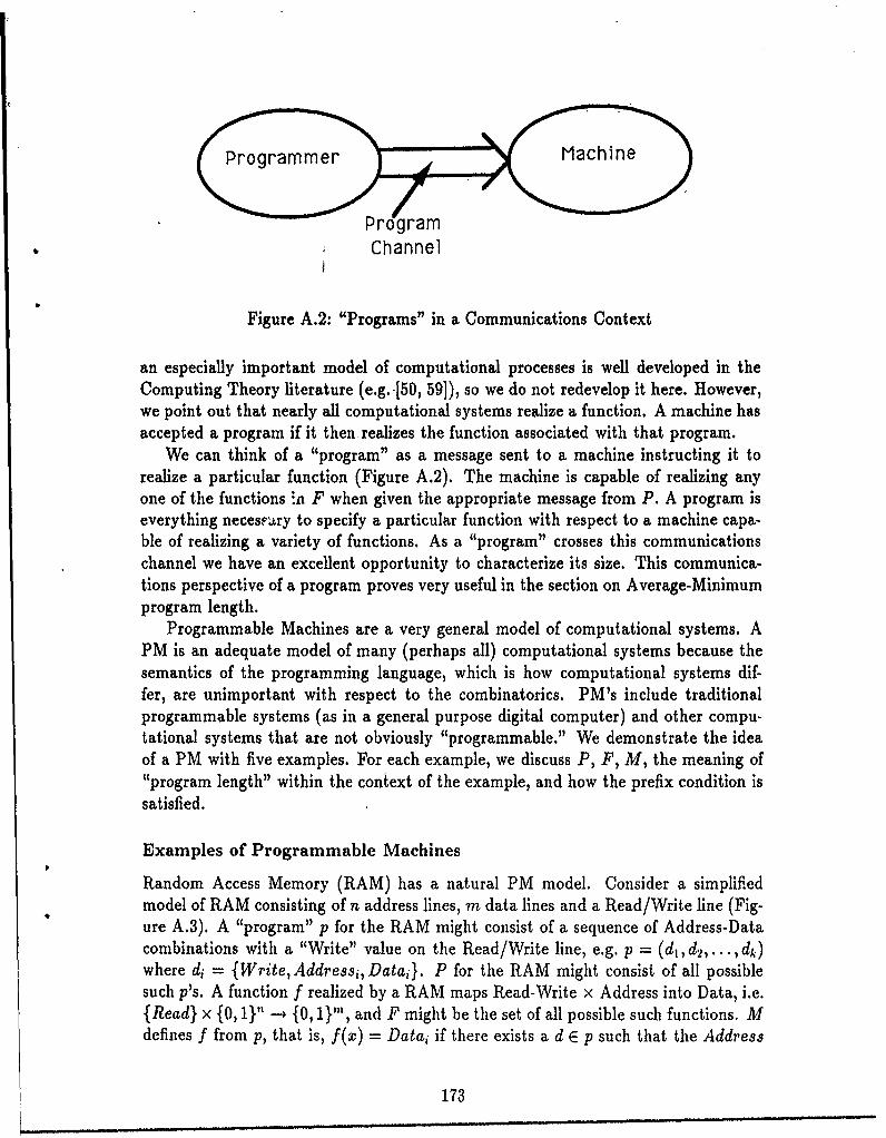
ProgramChannel

Figure A.2: "Programs" in a Communications Context

an especially important model of computational processes is well developed in theComputing Theory literature (e.g. [50, 59]), so we do not redevelop it here. However,we point out that nearly all computational systems realize a function. A machine hasaccepted a program if it then realizes the function associated with that program.

We can think of a "program" as a message sent to a machine instructing it torealize a particular function (Figure A.2). The machine is capable of realizing anyone of the functions in F when given the appropriate message from P. A program iseverything necessary to specify a particular function with respect to a machine capa-ble of realizing a variety of functions. As a "program" crosses this communicationschannel we have an excellent opportunity to characterize its size. This communica-tions perspective of a program proves very useful in the section on Average-Minimumprogram length.

Programmable Machines are a very general model of computational systems. APM is an adequate model of many (perhaps all) computational systems because thesemantics of the programming language, which is how computational systems dif-fer, are unimportant with respect to the combinatorics. PM's include traditionalprogrammable systems (as in a general purpose digital computer) and other compu-tational systems that are not obviously "programmable." We demonstrate the ideaof a PM with five examples. For each example, we discuss P, F, M, the meaning of"program length" within the context of the example, and how the prefix condition issatisfied.

Examples of Programmable Machines

Random Access Memory (RAM) has a natural PM model. Consider a simplifiedmodel of RAM consisting of n address lines, m data lines and a Read/Write line (Fig-ure A.3). A "program" p for the RAM might consist of a sequence of Address-Datacombinations with a "Write" value on the Read/Write line, e.g. p = (d1 , d2,... ,4 )where di = {Write, Addressj, Datai}. P for the RAM might consist of all possiblesuch p's. A function f realized by a RAM maps Read-Write x Address into Data, i.e.{Read} x {0, 1}" -- {0, 1}"', and F might be the set of all possible such functions. Mdefines f from p, that is, f(x) = Data if there exists a d E p such that the Address

173

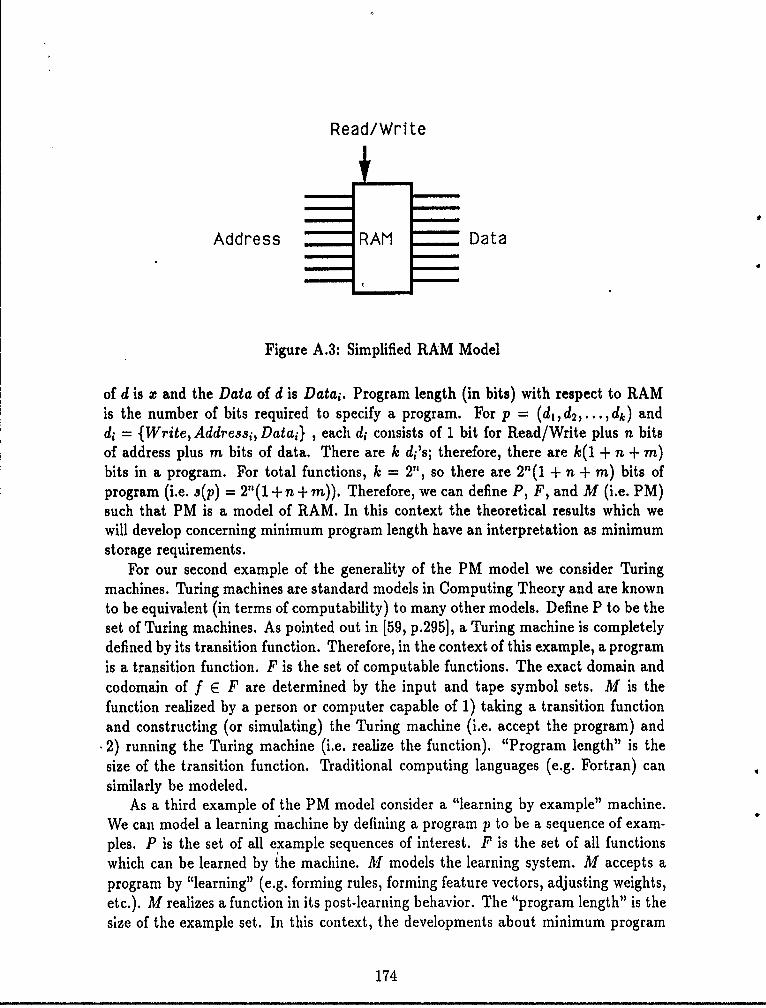
Read!Write

Address RAM Data

Figure A.3: Simplified RAM Model

of d is x and the Data of d is Datai. Program length (in bits) with respect to RAMis the number of bits required to specify a program. For p = (d,d 2,...,dk) anddi = {Write, Addressi, DataJ} , each di consists of 1 bit for Read/Write plus n bitsof address plus m bits of data. There are k di's; therefore, there are k(1 + n + m)bits in a program. For total functions, k = 2", so there are 2 n(1 + n + m) bits ofprogram (i.e. s(p) = 2"(1 + n + m)). Therefore, we can define P, F, and M (i.e. PM)such that PM is a model of RAM. In this context the theoretical results which wewill develop concerning minimum program length have an interpretation as minimumstorage requirements.

For our second example of the generality of the PM model we consider Turingmachines. Turing machines are standard models in Computing Theory and are knownto be equivalent (in terms of computability) to many other models. Define P to be theset of Turing machines. As pointed out in [59, p.295], a Turing machine is completelydefined by its transition function. Therefore, in the context of this example, a programis a transition function. F is the set of computable functions. The exact domain andcodomain of f E F are determined by the input and tape symbol sets. M is thefunction realized by a person or computer capable of 1) taking a transition functionand constructing (or simulating) the Turing machine (i.e. accept the program) and2) running the Turing machine (i.e. realize the function). "Program length" is the

size of the transition function. Traditional computing languages (e.g. Fortran) cansimilarly be modeled.

As a third example of the PM model consider a "learning by example" machine.We can model a learning machine by defining a program p to be a sequence of exam-pies. P is the set of all example sequences of interest. F is the set of all functionswhich can be learned by the machine. M models the learning system. M accepts aprogram by "learning" (e.g. forming rules, forming feature vectors, adjusting weights,etc.). M realizes a function in its post-learning behavior. The "program length" is thesize of the example set. In this context, the developments about minimum program

174

length and "programmability" become minimum example requirements and "learn-ability." This example could be adapted to other learning modes, where whatever itis that the machine learns from acts as the program.

In this example of a PM we connect "program length" with circuit complexity.Define a program to be the specification of a logic circuit. P is the set of all suchspecifications. F is the set of all functions of the form f : {0, 1}" --+{0, 1}. M is thefunction realized by 1) a person or automated manufacturing system which "acceptsa program" by constructing a circuit per the specifications and 2) the constructedcircuit which realizes a function. There are many ways in which a logic circuit mightbe specified (e.g. ((w AND x) OR ( NOT y)) AND z). However, any specificationmust identify the gates (e.g. AND, OR, NOT) and the interconnection of the gates.Therefore, program length (i.e. length of the circuit specification) is related to thecomplexity of the circuit (i.e. number of gates and number of interconnections). Inthis context, the developments concerning minimum program length become limitson minimum circuit complexity.

The discussion in the previous example did not depend on the circuits havingdiscrete values. Therefore we could define a PM for analog computing (electronic,acoustical, optical, etc.). Programs would reflect an identification of the componentsand their interconnection. F would be the set of functions realizable by some specifiedanalog computer.

Tabular Programs

There is a special form of program, for most machines, with the following charac-teristics. One, every function in F has a representation of this form and two, thelength of the program in this form is the same for every function in F. We call arepresentation of this form a tabular representation. A tabular representation is es-sentially an exhaustive list or table of the function's values. Revisiting the examplesabove, every RAM program is tabular. That is, every function has a program andall programs are the same length. With respect to a Turing Machine, a transitionfunction which includes a transition for each ordered pair of f (i.e. x and f(x)) isa tabular representation. In this case, as with the RAM, the size of the transitionfunction (program length) corresponds to the size of f (i.e. 8(p) 0C [f]). A tabularrepresentation with respect to a learning machine simply means that the "exampleset" is an exhaustive list of the ordered pairs of f. That is, there is an example inthe training set for each possible input. Again, the size of the example set (programlength) corresponds to the size of f. A tabular representation with respect to logiccircuits could be constructed using canonical forms. A tabular representation of afunction is a kind of the backstop of all representations.

The Set of Minimum Length Programs

As our final comment on machine models we identify a special subset of the set ofall programs. A program specifies which element of F that the machine is to realize.

175

Each program has exactly one function associated with t. However, each functionmay have zero, one, or more associated programs. That is, a given program can onlyrealize one function, but, a particular function may have any number of programs.Let Pmi,, a subset of P, consist of those elements of P which do not have a shorterprogram that realizes the same function.. That is,

Pmi. = {p E P I s(p) <_ s(q)Vq E P and M(p) = M(q)},

where M(p) indicates the function realized by p. A largest element of -P.in is denotedp', so that s(p') > s(p)Vp E Pmin. That is, p' is a largest program of P,,i, required torealize any realizable function of F. If s(p') is greater than some threshold (t) thenit immediately follows that there exists a program of length greater than t. That is,p' is a program of length greater than t. s(p') will be called the max-min programlength of set P with respect to M.

A.2.3 Maximum-Minimum Program Length for Finite andTransfinite Sets

The following theorem relates function set and program set cardinalities.

Theorem A.6 If (M,P, F) is a Programmable Machine then [P] > [F].

Proof:By definition of a function, each p E P can be associated with at most one f E F;or a particular program can only compute one function. Also, since M is onto F,there is a (p, f) pair for every f E F. Therefore, for every f E F there is at least oneunique p E Pmin and Pmin C P.0

This seems trivial. However, it is the basis for all the combinatorics based non-computability results. Now let p' denote the longest program in Pmin. Now we relatefunction set cardinality and program length.

Theorem A.7 If(M, P, F) is a Programmable Machine and the programs are strings

on an alphabet Ep of [Ep] letters then '( [F].

Proof:Theorem A.2 demonstrated that the set of all strings of length less than or equal to

s(p') is [ +- Therefore, any particular set P, with a longest string p', cannot

have more than[ -1 elements, i.e. [ >']- > [P]. This inequality and that

of Theorem A.6 gives us [ >,] [] [F].0

176

Theorem A.8 if(M, P, F) is a Programmable Machine and the programs are vectorson an alphabet EJp of [Ep] letters then [Ep]s(p) > IF].

Proof:Same as Theorem A.6, except replace the expression for the cardinality of a set ofstrings with the expression for the cardinality of a set of vectors (Theorem A.1).0

Theorem A.8 may be interpreted as an approximation of the constraint of The-orem A.7. This approximation is correct to within a factor of 2 by Theorem A.3.The discussion will use this simpler and essentially correct expression. We will call"6[Ep]a(P') > [F]" the first max-min program length constraint.

What does the first max-min program length constraint imply about the relation-ship between function cardinality [f] and program length s(p')? In general nothing.That is, the function set F and individual elements of F can have any combination ofcardinalities. For example, let the individual functions be of the form {(i,j)}, withij E N. In this example, [F] = N., while [f] = 1. On the other hand, suppose weare only interested in two functions, namely f(x) = x and g(z) = x + 1, each on theReals. In this case, [F] = 2, while If] = c. Therefore, in general, the combinatorialconstraint implies nothing about the relationship between function cardinality andmax-min program length.

Let us assume that the functions of interest are exactly all the total functions on agiven domain (X). This assumption creates a relationship between IF] and [f]. Thisallows us to use the combinatorial constraint to relate [f] and s(p').

Theorem A.9 If (M, P, F) is a Programmable Machine, the programs are stringson an alphabet Ep of [EJp] letters and F is the set of all total functions of the formf : X - Y then

[EPj(P 1)+I 1 > [y]X][EP] - I

Proof:By Theorem A.4 [F] - [Y][x]. Theorem A.9 then follows immediately from Theo-rem A.7.0

Theorem A.10 If (M, P, F) is a Programmable Machine, the programs are vectorson an alphabet EJp of [Ep] letters, F is the set of all total functions of the formf : X -f Y and [Y] = [Ep] then s(p') > [X].

Proo[E( I+- of Theorem A.9 is replaced by [Ep]s(P') as in Theorem ...8 to get [rpj(P') >

[Y1[1]. Since [Y = j)pp, a log of both sides gives s(p') >_ [X].

177

Note that [X] = [f] for total functions. When we are talking about decisionproblems (i.e. [Y] = 2) and a binary alphabet (i.e. [Ep] = 2), this expression applies.Again, by fixing some particulars and approximating the cardinality of a set of stringswe can simplify the expression and bc't !r reveal the essential relationships. We callthis the second max-min program length conbtraint.

A comparison between function cardinality and program length seems to be espe-cially natural. The representation of a function as a look-up table is always possible,although infinite functions require infinite tables. We can think of a table with alook-up capability as a "program" and the length of this program is exactly that ofthe function. This is the basis for many of the developments of Chapter 4.

We can think of the length of an input in two ways. The length of the input as thelength of a string might be one measure. For functions with inputs from N, the inputlength might be the value of the input. However, the set N and the set of finite lengthstrings have the same cardinality, therefore it makes no difference which approach weuse. Let us treat input length as the length of the string that expresses the input,and denote it s(x). Now what does the combinatorial constraint imply about therelationship between input length and program length? Again, in general nothing.That is, the function set F and an individual element f E F can have independentcardinalities (as indicated before) and the cardinality of an input X to f can beindependent of [f]. For the example with individual functions of the form {(i,j)},with ij E N, [F] = N. while s(x) = 1. On the other hand, for the two functions,f(x) = x and g(x) = x + 1, each on the Reals, [F] = 2 while s(x) = N,. Therefore, ingeneral, the combinatorial constraint implies nothing about the relationship betweeninput length and max-min program length.

We established in Theorem A.9 that, with an assumption about the form of thefunction set F, we could relate function cardinality [f I to function set cardinality [F].Now we introduce an additional assumption which allows us to relate input lengths(x) and function set cardinality [F]. Let us assume, as before, that the functions ofinterest are exactly all the total functions on a given domain X and codomain Y. Inaddition let us assume that the domain X is the set of all strings on an alphabet E.\.of [Ex) letters. The following theorem relates input length and program length.

Theorem A.11 If (M, P, F) is a Programmable Machine, the programs are stringson an alphabet Ep of [Ep] letters, F is the set of all total functions of the formf : X - Y and X is the set of all strings on Ex of length less than or equal to s(x')then

[P8(P()+i - 1 [ )+ L

(.,' - 1 -

or equivalently[pJs(p()+I -

p," - 178

178

Proof:From Theorem A.2, [X] = [X -1 Theorem A.11 then follows immediately fromTheorem A.9.0

Theorem A.12 If (M, P, F) is a Programmable Machine, the programs are stringson an alphabet IEp of [IEp] letters, F is the set of all total functions of the formf : X - Y and X is the set of all strings on EX of length less than or equal to s(aY)then s(p') > [Y.x"C).

Proof:By Theorem A.1 [X] = [x]\.(x'). The proof then follows from Theorem A.10.0

Again, the expression of the constraint can be greatly simplified by assumptionsand approximations in non-essential areas. Under these assumptions, if a machinecan realize all functions with input less than or equal to s(Z') then s(p') is greaterthan or equal to the power of input length, i.e. s(p') > [Ex]-(x'). This might alsobe expressed .(p') > [.]6(x)Vx E X. This is the third max-min program lengthconstraint.

The remainder of this section is a summary of the developments so far. Wediscussed the important role of simple combinatorics in deciding the max-min programlength. In particular, for there to exist a sufficient number of programs, at least onefor each function, the longest program must be at least a certain length. Another wayto express this is that there must exist a program of a certain length s(p') or longer.We developed three statements of this combinatorial constraint: 1) [Ep]j8(P') > [F],2) s(p') >_ [f], and 3) s(p') [.\]s(x)Vx E X. We called these the first, second andthird max-min program length constraints, respectively. We did not assume finitecardinalities in the development of these constraints; therefore, all the constraints arevalid for finite an .i transfinite cardinals.

The first statement says that there must exist a program whose length is greaterthan or equal to the number of elements in the set of functions that the machinecan be programmed to realize. This is the most general and most explicit of thethree statements. It is general in that it uses neither of the assumptions required forstatements 2 and 3. In particular, the functions and their domains are not assumedto be of a particular form. The first statement is more explicit in that it includes [F]and s(p'), which are the driving parameters of the problem. The other parameters(i.e. [f] or s(x)) determine s(p') only indirectly through [F], via the assumptions ofthe second and third statements.

The second statement says that there must exist a program with length greaterthan or equal to the number of elements in the functions that the machine can beprogrammed to realize. This statement requires that we assume a function set of acertain form. Therefore, it is not as general as the first statement. However, thisstatement has an attractive intuitive interpretation. A function is a set of cardinality

179

[f], therefore, it is reasonable to expect a representation of the function to be ofcardinality [f]. Furthermore, any function can be represented with a look-up table(although transfinite functions will require transfinite table sizes) and the size of thetable is exactly [f].

The third statement says that there must exist a program with length greater thanor equal to the power of the longest input string to the functions that the machine canbe programmed to realize. This statement requires two assumptions. One assumptionconcerns the functions' form relative to the domain. The other assumption concernsthe form of the domain itself. Therefore, this third statement is the least general ofthe three. These assumptions provide the necessary link back to [F]i however, [F] isnow twice removed in this expression. Therefore this third statement is also the leastexplicit.

Programmability

We have seen how the combinatorial constraint implies that "programs" must bea certain length if we are to realize a certain variety of functions. However, withthe machine model of Section A.2.1 we see that "program" has an unusually generalmeaning. For example, the combinatorial constraint implies that the specification ofa circuit must be so long if the specification format is sufficiently general to allowspecifying a certain variety of functions. Similarly, the combinatorial constraint im-plies that a certain minimum number of examples are required if a learning machineis to be capable of learning a certain variety of functions. The constraint even limitsthe expressability of a natural language in instructing a person in a task.

We would now like to develop the idea of "programmability." We assume thatwe have a set of functions (F) which we wish to be able to compute and a set ofprograms (P) which we are capable of generating. The programmability question thenis: "Does there exist a Programmable Machine which will map P into F?" Another,more traditional, way of viewing this problem is: "Does there exist an f E F whichcannot be programmed from P?" The previous results provide a sufficient conditionfor the existence of non-programmable functions.

Theorem A.13 Given a set of programs P and a set of functions F there exist anon-programmable function if [P] < [F].

Proof:There are more f's in F than there are p's in P and any given p can realize only onef.0

We can produce several variants of this result using the conditions of Theo-rems A.8, A.10, and A.12.

180

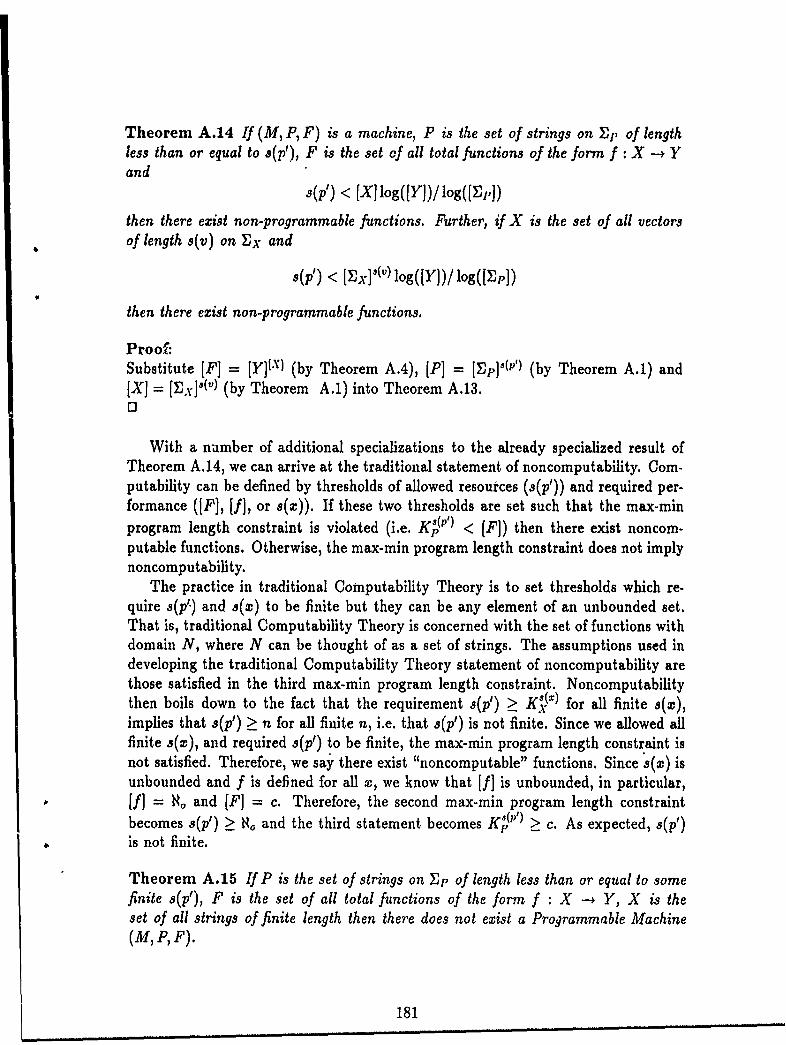
Theorem A.14 If (M, P, F) is a machine, P is the set of strings on Ejr of lengthless than or equal to s(p'), F is the set of all total functions of the form f : X -+ Yand 8(p') < [XjlogQYDl/log([r,,])then there exist non-programmable functions. Further, if X is the set of all vectorsof length s(v) on E2x and

s-0) < [EX]'t')log(Ir]/log[EP])

then there exist non-programmable functions.

Proof:Substitute [F] = [Y]I.') (by Theorem A.4), [P] = [Ep]'(P') (by Theorem A.1) and[XJ = [EP,- '(v)(by Theorem A.1) into Theorem A.13.

With a number of additional specializations to the already specialized result ofTheorem A.14, we can arrive at the traditional statement of noncomputability. Com-putability can be defined by thresholds of allowed resources (s(p')) and required per-formance ([F], [f], or s(x)). If these two thresholds are set such that the max-minprogram length constraint is violated (i.e. K p" ') < [F]) then there exist noncom-putable functions. Otherwise, the max-min program length constraint does not implynoncomputability.

The practice in traditional Computability Theory is to set thresholds which re-quire s(p') and s(x) to be finite but they can be any element of an unbounded set.That is, traditional Computability Theory is concerned with the set of functions withdomain N, where N can be thought of as a set of strings. The assumptions used indeveloping the traditional Computability Theory statement of noncomputability arethose satisfied in the third max-min program length constraint. Noncomputabilitythen boils down to the fact that the requirement s(p') > Ks!x) for all finite s(z),implies that s(p') > n for all finite n, i.e. that s(p') is not finite. Since we allowed allfinite s(x), and required s(p') to be finite, the max-min program length constraint isnot satisfied. Therefore, we say there exist "noncomputable" functions. Since s(x) isunbounded and f is defined for all x, we know that [f] is unbounded, in particular,[f] = R, and [F] = c. Therefore, the second max-min program length constraintbecomes s(p') > R,, and the third statement becomes K,)'() > c. As expected, s(p')is not finite.

Theorem A.15 If P is the set of strings on Ep of length less than or equal to somefinite s(p'), F is the set of all total functions of the form f : X -* Y, X is theset of all strings of finite length then there does not exist a Programmable Machine(M, P, F).

181

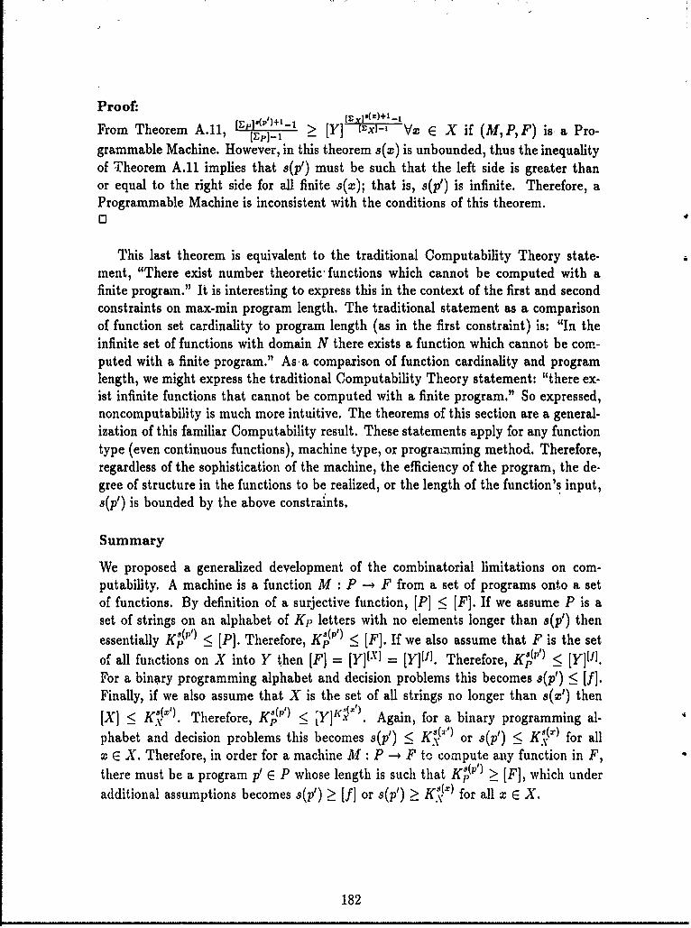
Proof:[ ](P')+ -1. Ix )+ -

From Theorem A.11, ]- _ [Y] L xJ-,FVX E X if (M, P,F) is a Pro-grammable Machine. However, in this theorem s(x) is unbounded, thus the inequalityof Theorem A.11 implies that s(p') must be such that the left side is greater thanor equal to the right side for all finite s(x); that is, s(p) is infinite. Therefore, aProgrammable Machine is inconsistent with the conditions of this theorem.o3

This last theorem is equivalent to the traditional Computability Theory state-ment, "There exist number theoretic functions which cannot be computed with afinite program." It is interesting to express this in the context of the first and secondconstraints on max-min program length. The traditional statement as a comparisonof function set cardinality to program length (as in the first constraint) is: "In theinfinite set of functions with domain N there exists a function which cannot be com-puted with a finite program." As a comparison of function cardinality and programlength, we might express the traditional Computability Theory statement: "there ex-ist infinite functions that cannot be computed with a finite program." So expressed,noncomputability is much more intuitive. The theorems of this section are a general-ization of this familiar Computability result. These statements apply for any functiontype (even continuous functions), machine type, or programiming method. Therefore,regardless of the sophistication of the machine, the efficiency of the program, the de-gree of structure in the functions to be realized, or the length of the function's input,s(p') is bounded by the above constraints.

Summary

We proposed a generalized development of the combinatorial limitations on com-putability. A machine is a function M : P -- F from a set of programs onto a setof functions. By definition of a surjective function, [P] _ [F]. If we assume P is aset of strings on an alphabet of Kp letters with no elements longer than 8(p') thenessentially K '" ) < [P]. Therefore, K p' ) [F]. If we also assume that F is the setof all functions on X into Y then [F] = [Y]-\' = [Yjfl. Therefore, K,("') < [Yj!JJ.For a binary programming alphabet and decision problems this becomes s(p') :_ [f].Finally, if we also assume that X is the set of all strings no longer than s(z') then

_ j":' K (° yjK (').[X] < K. K ". Therefore, K' < . Again, for a binary programming al-phabet and decision problems this becomes s(p') < Ah'') or s(p') < Ka(x) for allx E X. Therefore, in order for a machine M : P -- F to compute any function in F,there must be a program p' E P whose length is such that g p ') > [F], which underadditional assumptions becomes s(p') If] or s(p') , 1x) for all x E X.

182

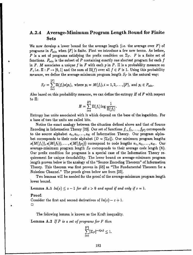
A.2.4 Average-Minimum Program Length Bound for FiniteSets

We now develop a lower bound for the average length (i.e. the average over F) ofprograms in Pmin when [F] is finite. First we introduce a few new terms. As before,P is a set of programs satisfying the prefix condition on Ep. F is a finite set offunctions. Pmi, is the subset of P containing exactly one shortest program for each fin F. M associates a unique f in F with each p in P. 11 is a probability measure onF, i.e. 11 : F --+ [0, 1] and the sum of H1(f) over all f E F is 1. Using this probabilitymeasure, we define the average-minimum program length SF in the natural way:

SF= >3I(fi)s(pi), where pi = M(fi), i = 1,2,.. ., [F], and Pi E P,i,,.i=1

Also based on this probability measure, we can define the entropy H of F with respectto 11:

IF]H = >3n(fi)log .(f).

Entropy has units associated with it which depend on the base of the logarithm. Fora base of two the units are called bits.

Notice the exact analogy between the situation defined above and that of SourceEncoding in Information Theory [23]. Our set of functions fl, f 2,... , fir] correspondsto the source alphabet at,a 2,... , aK of Information Theory. Our program alpha-bet corresponds to their code alphabet (D = [Ep]). Our minimum program lengthss(M(fi)),a(M(f 2)),...,s(M(f(Fj)) correspond to code lengths nl,n 2 ,...,nK. Ouraverage-minimum program length SF corresponds to their average code length (i).Our prefix condition for programs is a special case of the Information Theory re-quirement for unique decodability. The lower bound on average-minimum programlength proven below is the analogy of the "Source Encoding Theorem" of InformationTheory. This theorem was first proven in [56] as "The Fundamental Theorem for aNoiseless Channel." The proofs given below are from [23].

Two lemmas will be needed for the proof of the average-minimum program lengthlower bound.

Lemma A.1 ln(z) < z - 1 for all z > 0 and equal if and only if z = 1.

Proof:Consider the first and second derivatives of ln(z) - z + 1.0

The following lemma is known as the Kraft inequality.

Lemma A.2 If P is a set of programs for F then

IF] ~< 1i=1

183

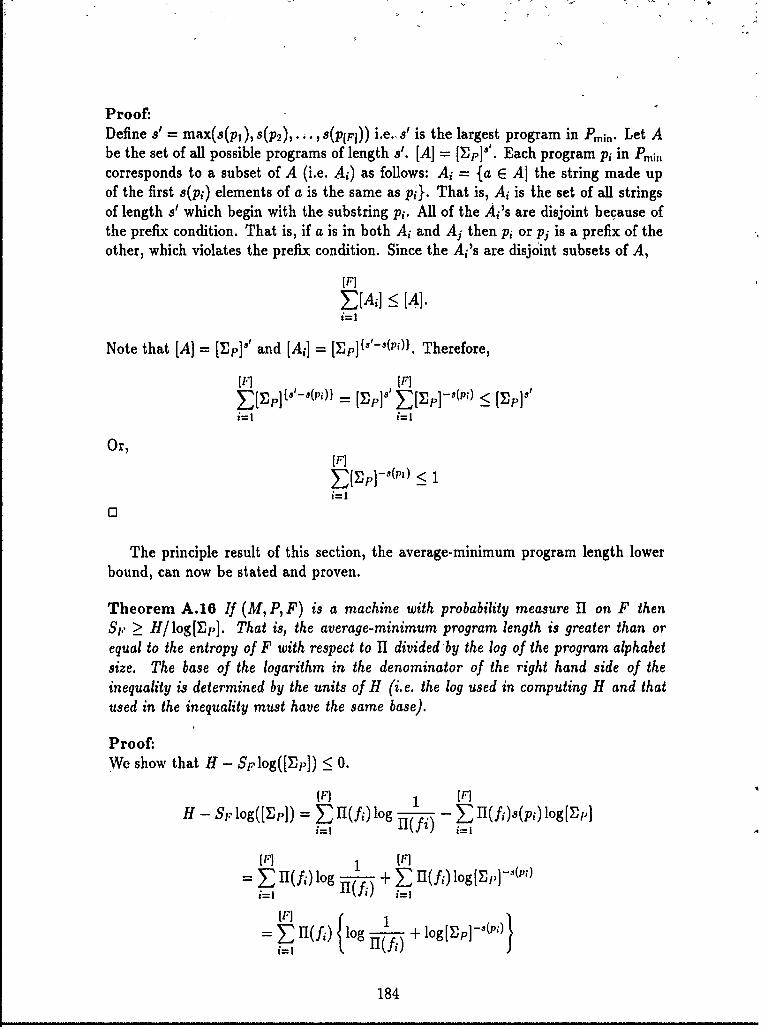
Proof:Define ' = max(s(p1 ),s(p2),. . ,S(p(F])) i.e., a' is the largest program in P,. Let Abe the set of all possible programs of length s'. [A] = [Ep]'. Each program pi in P ..hjcorresponds to a subset of A (i.e. Ai) as follows: Ai = {a E Al the string made upof the first s(pi) elements of a is the same as pi). That is, Ai is the set of all stringsof length s' which begin with the substring pi. All of the Ai's are disjoint because ofthe prefix condition. That is, if a is in both Ai and Aj then pi or pj is a prefix of theother, which violates the prefix condition. Since the Ai's are disjoint subsets of A,

['1[A,] <141].

Note that [A] = [EpV' and [Ai] = [E}]{'-$(P)}. Therefore,

I'.'] [F]

=F [E]'Z rJ]-(l I~Vi E i= 1

Or,[F]

i=I1

0

The principle result of this section, the average-minimum program length lowerbound, can now be stated and proven.

Theorem A.16 If (M, P, F) is a machine with probability measure II on F thenSp > H/log[']p]. That is, the average-minimum program length is greater than orequal to the entropy of F with respect to II divided by the log of the program alphabetsize. The base of the logarithm in the denominator of the right hand side of theinequality is determined by the units of H (i.e. the log used in computing H and thatused in the inequality must have the same base).

Proof:We show that H - Splog([]p]) < 0.

[F 1 [F]

H - SFlog([EP]) = HL(h )log - 1(fi)S(Pi)log[EP]i~~l II(fi) i

[]1 [F]

- U (fi) log f + L II(f) log[,]l-("')i=I IIJi) i= I

- II())log + log[EpI - (Pi)}I=,184

184

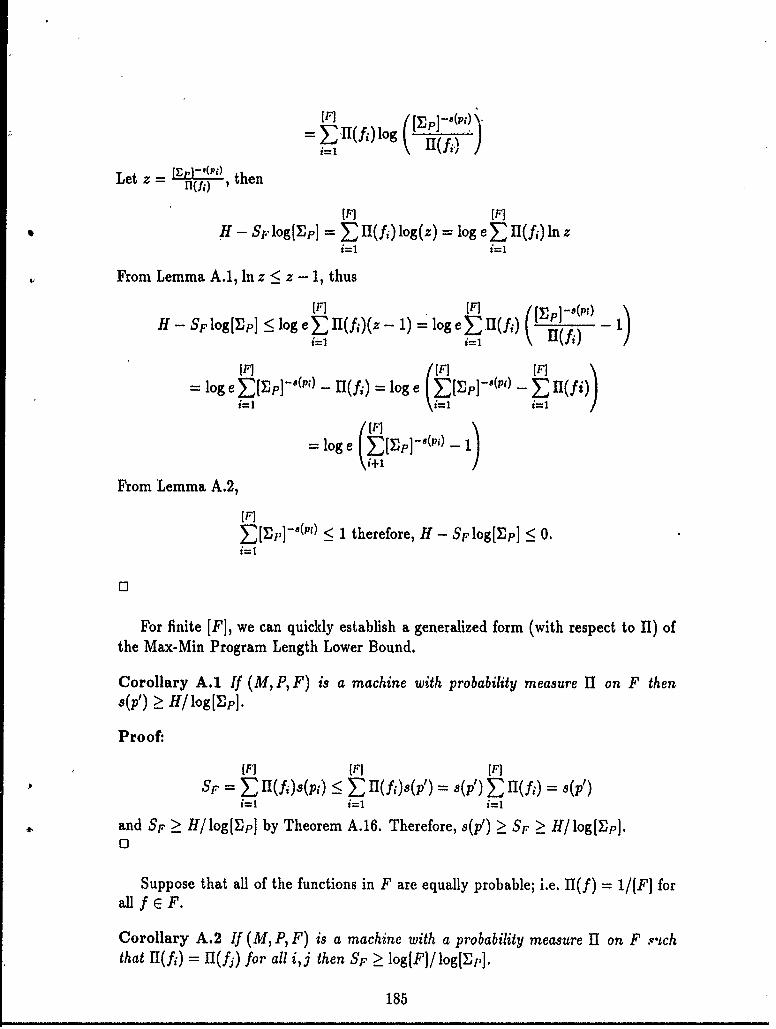
-Z"(f,)log

Letz= hen ,

[F] IF]

H - Splog[Ep] = r(f/i) log(z) = log e 11(f,)lnzi=1 i=1

From Lemma A.1, In z < z - 1, thustI , III ( [E ]- ("'O '

H - SFlo[Ep] < log eZI(fj)(z- 1) = loge HI(A)Cf)1

[F] [ F(f]

I[II. IF-,( ) 1F)=log e [Ep](Pi) - 11(fj) = log e Eip")- E 11(i))

log e p[](P) -

From Lemma A.2,

[F]

Z[Fp] -B() < 1 therefore, H - Splog[Ep] < 0.i=1

0

For finite [F], we can quickly establish a generalized form (with respect to H) ofthe Max-Min Program Length Lower Bound.

Corollary A.1 If (M, P, F) is a machine with probability measure 1I on F thens(p') > H/log[Ep].

Proof:

IF] IF] [F]

Sr = (f,)s(pi) <_ j(f,)s(p') = q(p') Z1(f) = 9(p')i=1 i=l i=1

and SF _ H/log[Ep] by Theorem A.16. Therefore, s(p') > SF _ H/log[Ep].0

Suppose that all of the functions in F are equally probable; i.e. 1(f) = 1/[F] forall f E F.

Corollary A.2 If (M, P, F) is a machine with a probability measure H1 on F -ichthat II(f;) = I(f,) for all ij then SF > log[F]/log[Ep],

185

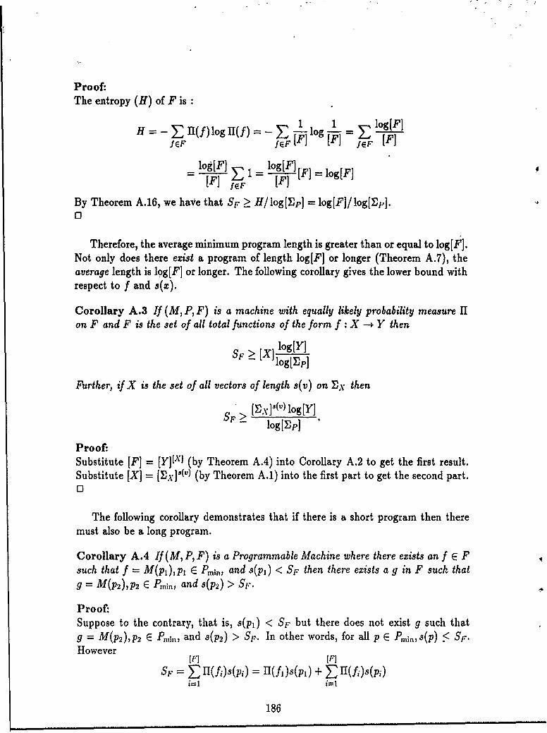
Proof:The entropy (H) of F is

s~r 1 log[F]H -- (f)logll(f)- -- l lo = l[F]

JEF fEF [] F] fEF F

log[F= log[F]

- [F] 1 -F [F]

By Theorem A.16, we have that SF > H/log[Ep] = log[F]/log[Ep].0

Therefore, the average minimum program length is greater than or equal to log[F].Not only does there exist a program of length log[F] or longer (Theorem A.7), theaverage length is log[F] or longer. The following corollary gives the lower bound withrespect to f and s(x).

Corollary A.3 If (M, P, F) is a machine with equally likely probability measure H1on F and F is the set of all total functions of the form f : X --+ Y then

SF [AX log[Y]log [EP]

Further, if X is the set of all vectors of length s(v) on Ex then

SF > [E .y](V) log[Y ] .

log[EJp]

Proof:Substitute [F] = [Y]LXJ (by Theorem A.4) into Corollary A.2 to get the first result.Substitute [X] = [Fx]s(v) (by Theorem A.1) into the first part to get the second part.01

The following corollary demonstrates that if there is a short program then theremust also be a long program.

Corollary A.4 If(M, P, F) is a Programmable Machine where there exists an f E Fsuch that f = M(pl),p, E Pm., and s(pl) < Sr then there exists a g in F such thatg = M(p 2 ),P 2 E Pmin, and 8(p2) > Srl.

Proof-Suppose to the contrary, that is, s(pi) < Sp but there does not exist g such thatg = M(p 2 ),p 2 E P,,,j,, and 8(p2) > S1,. In other words, for all p E Pmin,S(p) :5 SF.However

[F] [F]

sF= I (fi)s(pi)= (I)s(p) + Z (fi)s(pi)=1 i=1

186

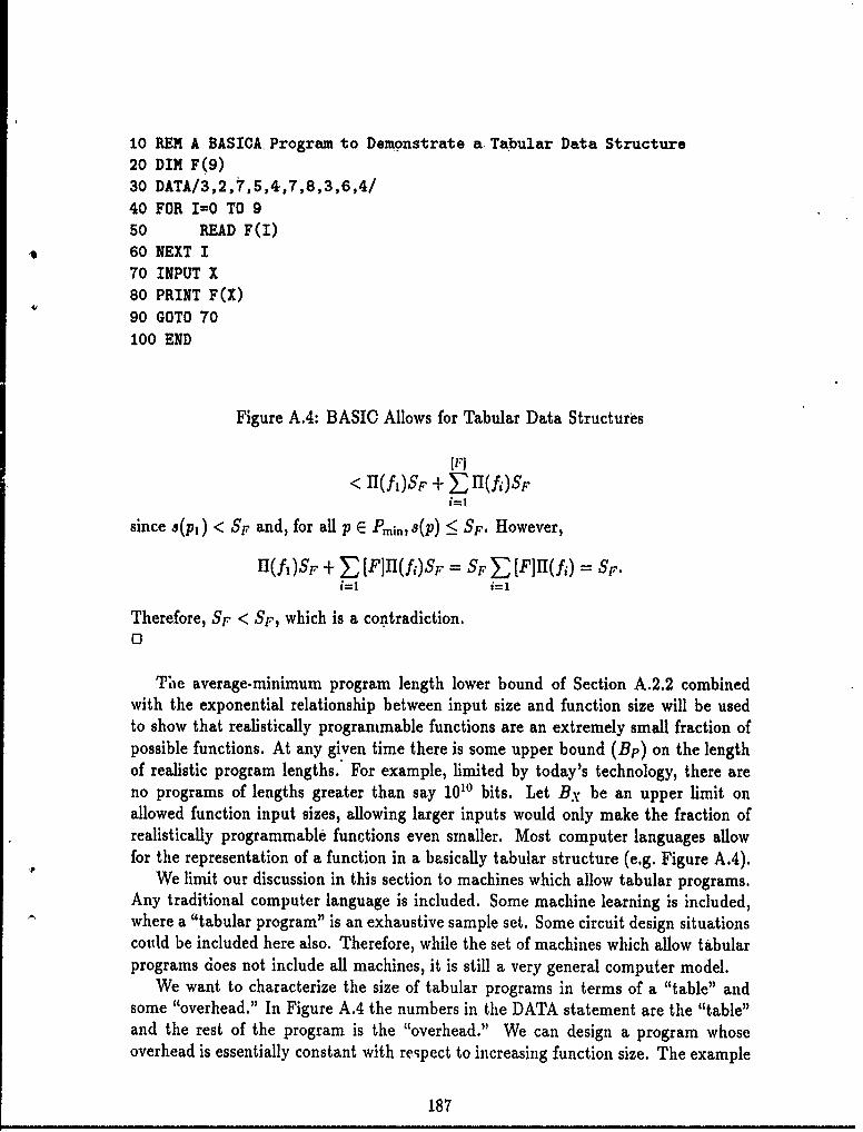
10 REM A BASICA Program to Demonstrate a Tabular Data Structure20 DIM F(9)30 DATA/3,2,7,5,4,7,8,3,6,4/40 FOR I=O TO 950 READ F(I)60 NEXT I

70 INPUT X80 PRINT F(X)90 GOTO 70100 END

Figure A.4: BASIC Allows for Tabular Data Structures

[F]

< 1(fi)S + II(i)SF

since s(pl) < SF and, for all p E Pmin,s(P) < SF. However,

(fl)SF + =[F]II(f)SF Sp [F]II(fi) = Sr.i=1 i=1

Therefore, SF < SF, which is a contradiction.0

The average-minimum program length lower bound of Section A.2.2 combinedwith the exponential relationship between input size and function size will be usedto show that realistically programmable functions are an extremely small fraction ofpossible functions. At any given time there is some upper bound (Bp) on the lengthof realistic program lengths. For example, limited by today's technology, there areno programs of lengths greater than say 1010 bits. Let Bx be an upper limit onallowed function input sizes, allowing larger inputs would only make the fraction ofrealistically programmable functions even smaller. Most computer languages allowfor the representation of a function in a basically tabular structure (e.g. Figure A.4).

We limit our discussion in this section to machines which allow tabular programs.Any traditional computer language is included. Some machine learning is included,where a "tabular program" is an exhaustive sample set. Some circuit design situationscould be included here also. Therefore, while the set of machines which allow tabularprograms does not include all machines, it is still a very general computer model.

We want to characterize the size of tabular programs in terms of a "table" andsome "overhead." In Figure A.4 the numbers in the DATA statement are the "table"and the rest of the program is the "overhead." We can design a program whoseoverhead is essentially constant with respect to increasing function size. The example

187

in Figure A.4 requires changing the DIM and FOR statements (these grow as thelog of function size); however, it is possible to design around such statements. DefineM' to be the set of machines which allow programs with lengths < [f] + K, for anyf and some constant K. Let F be a set of functions on inputs of length B.Y. Let G(the "good" functions) be the subset of F such that

G = {f E F13p E f = M'(p) implies that s(p) :_ Bp}.

Define R = [G]/[FJ, the fraction of F with programs of length Bp or less. Thisfraction of realistically computable functions is very small.

Theorem A.17 For any machine in M', R < K

Proof:Let St be the average-minimum program length of the set of functions . We areespecially concerned with SF, SG and SF-G.

SF [G]SG + [F - G]SF-G[F]

RSG + (1 - R)SFG

Since every function in f has a tabular program of cost [f] + K, the average-minimumcost over F (or any subset of F) cannot exceed this. Therefore,

SF-G <_. [f] + K = [,XIBx + K

andSG < Bp

from the definition of Bp. Substituting these relations into the expression for SF:

Sp = RS0 + (1 - R)SP-a _< R(Bp) + (1 - R)([E.] Bx + K)

From Theorem A.16, SF > [f] = [E.-]B.x. Therefore,

[E.\.]x < SF < R(BP) + (1 - R)([Ex]Bx + K)

[+J.]BX < R(Bp) + [XlBx + K - R([ExIjBx + K),

K > R(Bp - [,.\]B, + K).

Therefore,

KR [E .]Bx - Bp + K"

We see that the fraction of 'good' (i.e. realistically programmable) functions goesas the inverse of the difference between the bound in program size (Bp) and the bound

188

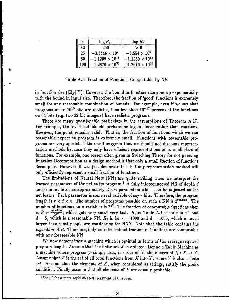
n log R1 log R 2

12 -256 >.025 -3.3546 x 1 -8.554 x 10650 -1.1259 x 10"s -1.1259 x 10'"

100 -1.2676 × 1030 -1.2676 x 103'

Table A.1: Fraction of Functions Computable by NN

in function size ([ .x]Bx). However, the bound in fwction size goes up exponentigilywith the bound in input size. Therefore, the fract on of 'good' functions is extremelysmall for any reasonable combination of bounds. For example, even if we say thatprograms up to 1010 bits are realistic, then less than 10- 12 percent of the functionson 64 bits (e.g. two 32 bit integers) have realistic programs.

There are many questionable particulars in the assumptions of Theorem A.17.For example, the 'overhead' should perhaps be log or linear rather than constant.However, the point remains valid. That is, the fraction of functions which we canreasonable expect to program is extremely small. Functions with reasonable pro-grams are very special. This result suggests that we should not discount represen-tation methods because they only have efficient representations on a small class offunctions. For example, one reason often given in Switching Theory for not pursuingFunction Decomposition as a design method is that only a small fraction of functionsdecompose. However, it was just demonstrated that any representation method willonly efficiently represent a small fraction of functions.

The limitations of Neural Nets (NN) are quite striking when we interpret thelearned parameters of the net as its program.' A fully interconnected NN of depth dand n input bits has approximately d x n parameters which can be adjusted as thenet learns. Each parameter is some real variable of say r bits. Therefore, the programlength is r x d x n. The number of programs possible on such a NN is 2rd~n. Thenumber of functions on n variables is 22". The fraction of computable functions then

2 rxdxnis R = 2--; which gets very small very fast. R, in Table A.1 is for r = 64 andd = 5, which is a reasonable NN. R 2 is for r = 1000 and d = 1000, which is muchlarger than most people are considering for NN's. Note that the table contains thelogarithm of R. Therefore, only an infinitesimal fraction of l'unctions are computablewith any foreseeable NN.

We now demonstrate a machine which is optimal in terms of fhc average requiredprogram length. Assume that the finite set X is ordered. Define a Table Machine asa machine whose program pi simply lists, in order of X, the images of fi : X -4 Y.Assume that F is the set of all total functions from X into Y, where Y is also a finites-'t. Assume that the elements of X, when considered as strings, satisfy the prefixcco1dition. Finally assume that all elements of F are equally probable.

'See [2] for a more sophisticated treatment of this idea.

189

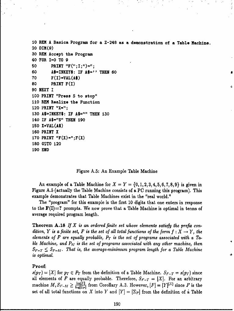
10 REM A Basica Program for a Z-248 as a demonstration of a Table Machine.20 DIM(9)30 REM Accept the Program40 FOR I=O TO 950 PRINT 'IF(";I;")=";60 A$INKEY$: IF A$'' THEN 6070 F(I)=VAL(A$)80 PRINT F(I)90 NEXT I100 PRINT "Press S to stop"110 REM Realize the Function120 PRINT "Xu";130 A$INKEY$: IF A$="" THEN 130140 IF A$="S" THEN 190150 X=VAL(A$)160 PRINT X170 PRINT "F(X)=";F(X)180 GOTO 120190 END

Figure A.5: An Example Table Machine

An example of a Table Machine for X = Y = {0,1, 2,3,4,5,6,7,8,9} is given inFigure A.5 (actually the Table Machine consists of a PC running this program). Thisexample demonstrates that Table Machines exist in the "real world."

The "program" for this example is the first 10 digits that one enters in responseto the F(I)=? prompts. We now prove that a Table Machine is optimal in terms ofaverage required program length.

Theorem A.18 If X is an ordered finite set whose elements satisfy the prefix con-dition, Y is a finite set, F is the set of all total functions of the form f : X -- Y, theelements of F are equally probable, PT is the set of programs associated with a Ta-ble Machine, and PA, is the set of programs associated with any other machine, thenSF-T < S-...A That is, the average-minimum program length for a Table Machineis optimal.

Proof:s(p'r) = [XI for P7 E PT from the definition of a Table Machine. SF-T = s(pT) sinceall elements of F are equally probable. Therefore, S.-T = [X]. For an arbitrarymachine M, S--Al > !1] from Corollary A.3. However, [F] = [Y]('J since F is thelog[ ,]set of all total functions on X into Y and [Y] = [Ep] from the definition of i Table

190

Machine. Then,

log[F = [X] log[Ep] and Sr-Ai > X logEe]-log[r~J]

Therefore, SF-A > [X] = SF-T.0

One consequence of this theorem is that "powerful" languages (e.g. Fortran is more"powerful" than a machine language) do not lessen the average-minimum programlength. The intuition that more powerful languages should allow a simpler expres-sion of a relationship is shown to depend a non-equally probable distribution of thefunction set. This suggests a connection between language design and some assumed(at least implicitly) probability distribution on F.

Theorem A.19 establishes that the bounds of Theorem A.16, Corollary A.2 andCorollary A.3 are the greatest lower bounds when the assumptions of Theorem A.18are met.

Theorem A.19 If the conditions of Theorem A,18 are met, thr ihe lower bounds ofTheorem A.i 6, Corollary A. 2 and Corollary A. 3 are greaiest- lower bounds of average-minimum program length.

Proof:If there were a greater lower bound then it would be violated by a Table Machine.0

A.3 Summary

This appendix develops a theory of computational complexity based on programlength. We formally defined our concept of programmable machine and proved nu-merous properties of program length. A programmable machine is sufficiently abstractto include many different kinds of problems. Under various interpretations the pro.gram length results become memory requirements, learnability, or circuit complexityresults. In effect, we have brought into an engineering setting some of the devel-opments of Shannon, Turing, C1h-itin and others. This common setting then hasextended applications, such as learnability, circuit complexity and especially PatternTheory.

191

Appendix B

Function Decomposition ProgramUser's Guide

This software is located in ficsim::user2:[vogt]'. There are 10 (that's right 10) differ-ent versions characterized as follows:

V.1. (8): Non-shared, exhaustiveV.2. (2): Non-shared, negative decompositionsV.2A. (0): Non-shared, negative decompositions,

greedy searchV.2B. (3): Non-shared, negative decompositions,

number of cares costV.2AB. (1): Non-shared, negative decompositions,

number of cares cost, greedyV.3. (9): Shared, exhaustiveV.4. (6): Shared, negative decompositionsV.4A. (4): Shared, negative decompositions,

greedy searchV.4B. (7): Shared, negative decompositions,

number of cares costV.4AB. (5): Shared, negative decompositions,

number of cares cost, greedy

The numbers in parentheses indicate relative speed, with V.2A being the fastestand V.3 the slowest. These are only rough estimates, and may even be slightly wrong.

To run the program, get into the directory appropriate to the version you wantto run, e.g.

$ set def [vogt.pbml.v4ab]

and then type

'This User's Guide was written by Chris Vogt.

193

run pbml-driver

It's that simple. The program will then come up with the following prompt:

SPECIFY FUNCTION TABLE VALUES:

Enter 0 to input from a file, i from terminal,

or 2 to QUIT program:

Interactive InterfaceTo enter the function in question interactively, enter a 1. The program will then

prompt you for the information needed. The prompts are relatively staightforward.A sample session to input a "checkerboard" on 3 variables (i.e. 01011010) is shownbelow:

Name of function: checkerboard3How many input variables does the function have?3

Enter 0 to input falses, 1 to enter trues: 1How many function values will you be entering? 4Enter negative values below for Don't CaresEnter decimal equivalent of binary input that has a true value: IEnter decimal.equivalent of binary input that has a true value: 3Enter decimal equivalent of binary input that has a true value: 4Enter decimal equivalent of binary input that has a true value: 6

To enter "don't care" values, use a negative number. For example, if we wanted toenter the function 010X1010, we would have typed -3 instead of 3.Input From a FileIf you are going to be using a function often, it may be handy to store it in a file.To input a function from a file, type 0 to the first prompt. The program will then

prompt you for the file name. Make sure you give the full file specification needed, orthe program will crash. The function is stored in the file with the following format:The first n + 1 digits indicate the number of input variables in unary. The next 2n

digits are the function itself. Thus, the file for the checkerboard entered above wouldbe:

01

1001011

194

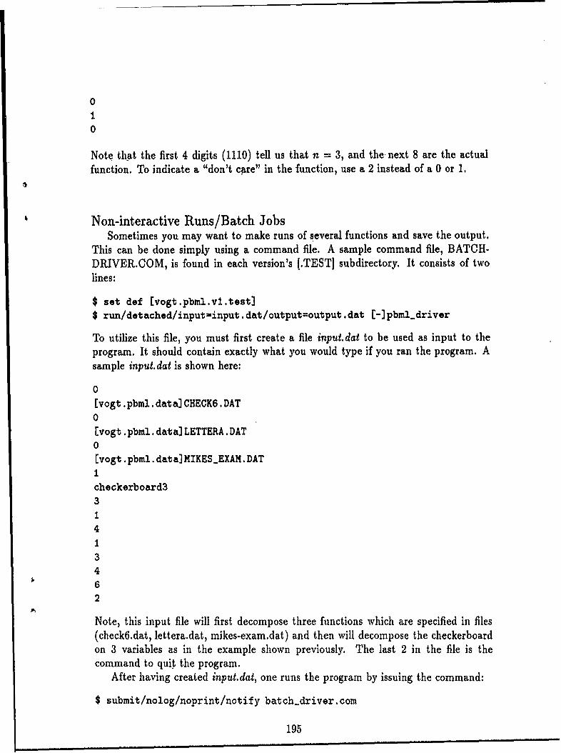
0

0

Note that the first 4 digits (1110) tell us that n = 3, and the next 8 are the actualfunction. To indicate a "don't care" in the function, use a 2 instead of a 0 or 1,

Non-interactive Runs/Batch JobsSometimes you may want to make runs of several functions and save the output.

This can be done simply using a command file. A sample command file, BATCH-DRIVER.COM, is found in each version's [.TEST] subdirectory. It consists of twolines:

$ set def [vogt.pbml.vl.test)$ run/detached/inputrinput.dat/output=output.dat [-]pbml-driver

To utilize this file, you must first create a file input.dat to be used as input to theprogram. It should contain exactly what you would type if you ran the program. Asample input.dat is shown here:

0[vogt.pbml. data) CHECK6.DAT0[vogt. pbml. data) LETTERA.DAT0[vogt. pbml. data) MIKESEXAM.DATIcheckerboard331413462

Note, this input file will first decompose three functions which are specified in files(check6.dat, lettera.dat, mikes-exam.dat) and then will decompose the checkerboardon 3 variables as in the example shown previously. The last 2 in the file is thecommand to quit the program.

After having created input.dat, one runs the program by issuing the command:

$ submit/nolog/noprint/notify batch-driver.com

195

The output from the program will be saved in the file output. dat, which will not beaccessible until the program is done running.

RecompilationIf changes are made to the source code, recompilation is simple. In each ver-

sion's directory, there is a corn file called comp*.com which does the job. The* isreplaced with the version number. Thus, in [vogt.pbml.v2ab] there is a file calledcompv2ab.com. This file can be executed interactively (with the @ sign), or can besubmitted as a batch job.

Two WARNINGS about recompiling:

e At present there is just barely enough disk quota to handle all of the filescreated during compilation. You need about 1300 blocks free, so check thequota beforehand.

* After compiling, to get rid of all of the "unnecessary" files created, execute thecommand file killada.com found in [vogt.com].

196

Bibliography

[1] Thomas Abraham. Pattern Recognition: Machine vs. Man. Final Report,USAF-UES Summer Faculty Research Program, July 1990.

(2] Ysar S. Abu-Mostafa. Information theory, complexity and neural networks.IEEE Communications Magazine, 27(11):25-28, 1989.

[3] A. V. Aho, J. E. Hopcroft, and J. D. Ullman. Data Structures and Algorithms.Addison-Wesley, Reading, Massachusetts, 1983.

(4] Robert L. Ashenhurst. The decomposition of switching functions. In Proceedingsof the International Symposium on the Theory of Switching, April 1957. Alsoin The Annals of the Harvard Computational Laboratory XXXIX, Harvard Uni-versity Press, Cambridge, Massachusetts, 1959, pages 74-116, and in Curtis'62pages 571-602.

[5] Mark Boeke. Pattern Based Machine Learning. Final Report, AFOSR HighSchool Apprenticeship Program, August 1990.

[6] John D. Bransford and Barry S. Stein. The IDEAL Problem Solver. W. H.Freeman and Company, New York, 1984.

[71 Gilles Brassard and Paul Bratley. Algorithmics: Theory and Practice. PrenticeHall, Englewood Cliffs, New Jersey, 1988.

[8] Mike Breen. Some Results in Pattern-Based Machine Learning. Final Report,USAF Summer Faculty Research Program, 1990.

[91 Richard Burden and J. Faires. Numerical Analysis. Prindle, Weber and Schmidt,

Boston, third edition, 1985.

[10] Maureen Caudill. Neural networks primer. Al Expert, 3(6):53-59, June 1988.

[11] Michael Chabinyc. Pattern Based Machine Learning: A Comparison of AdaFunction Decomposer Versions. Final Report, AFOSR High School Apprentice-ship Program, August 1990.

[12] Gregory. J. Chaitin. Algorithmic Information Theory. Cambridge UniversityPress, New York, 1987.

197

[13] Paul R. Cohen and Edward A. Feigenbaum, editors. The Handbook of ArtificialIntelligence. Addison-Wesley, Reading, Massachusetts, 1982.

[14] H. Allen Curtis. A New Approach to The Design of Switching Circuits. D. VanNostrand Company, Princeton, New Jersey, 1962.

[15] Lawrence Davis. Genetic Algorithms and Simulated Annealing. Morgan Kauf-mann, Palo Alto, California, 1987.

[16] Pierre A. Devijver and Josef Kittler. Pattern Recognition: A Statistical Ap-proach. Prentice Hall, Englewood Cliffs, New Jersey, 1982.

[17] D. Henry Edel. Introduction to Creative Design. Prentice Hall, Englewood Cliffs,New Jersey, 1967.

[18] Michael J. Findler. Neural Networks and Machine Learning. Graduate StudentResearch Program Final Report, Air Force Office of Scientific Research, August1989.

[19] M. J. Fischer and N. Pippenger. M. J. Fischer Lecture Notes on Network Com-plexity. Universitat Frankfurt, Frankfurt, 1974.

[20] A. A. Fraenkel. Abstract Set Theory. North-Holland Publishing Company, Am-sterdam, 1953.

[21] Arthur D. Friedman. Fundamentals of Logic Design and Switching Theory. Com-puter Science Press, Rockville, Maryland, 1986.

[22] King Sun Fu. Syntactic Pattern Recognition and Applications. Prentice Hall,Englewood Cliffs, New Jersey, 1982.

(23] R. Gallager. Information Theory and Reliable Communications. Wiley, NewYork, 1968.

[24] Wendell Garner. Good patterns have few alternatives. In I. Janis, editor, Cur-rent Trends in Psychology, pages 185-192, William Kaufmann Inc., Los Altos,California, 1977.

[25] Thomas K. Gearhart. Investigations of a Lower Bound on the Error in LearnedFunctions. Final Report, USAF-UES Summer Faculty Research Program, July1990.

1261 Donald D. Oivoiw. ntroduictimi to Snitchin Circuit Theory. Mc'raw-llI, NewYork, 1970.

[27] Gilbert Held and Thomas Marshall. Data Compression. Wiley, New York, sec-ond edition, 1987.

[28] Vladimir Hubka. Theory of Technical Systems. Springer-Verlag, New York, 1988.

198

(291 Laveen N. Kanal. Patterns in pattern recognition: 1968-1974. IEEE Transac-tions on Information Theory, 20:697-722, November 1974.

[301 John Langenderfer. A Study of the Computational Complexities of Functionsand their Inverses. Memorandum, Wright Research and Development Center,WL/AART Wright Patterson AFB, OH, September 1989.

[311 Pat Langley, editor. Proceedings of the Fourth Puternational Workshop on Ma-chine Learning, Morgan Kaufmann, Palo Alto, California, 1987.

[32] Pat Langley, Herbert A. Simon, Gary L. Bradshaw, and Jan M. Zytkow. Scien-tific Discovery: Computational Explorations of the Creative Process. The MITPress, Cambridge, Massachusetts, 1987.

[33] Ming Li and Paul M. B. Vitanyi. Kolmogorov complexity and its applications. InJan Van Leeuwen, editor, Handbook of Theoretical Computer Science, chapter 4,pages 189-254, The MIT Press, Cambridge, Massachusetts, 1990.

[34] 0. B. Lupanov. A method of circuit synthesis. Izv. V.U.Z. Radiofiz., 1(1):120-140, 1958.

[35] M. Machtey and P. R. Young. Theory of Algorithms. Elsevier North-Holland,New York, 1978.

[36] Peter S. Maybeck. Stochastic Models, Estimation and Control. Volume 1, Aca-demic 'Press, New York, 1979.

[37] Peter S. Maybeck. Stochastic Models, Estimation and Control. Volume 2, Aca-demic Press, New York, 1982.

(38] Loren P. Meissner. The Science of Computing. Wadsworth Publishing, Belmont,California, 1974.

(39] James L. Melsa and David L. Cohn. Decision and Estimation Theory. McGraw-

Hill, New York, 1978.

[40] J. L. Meriam. Statics. Wiley, New York, second edition, 1971.

[411 Paul L. Meyer. Introductory Probability and Statistical Applications. Addison-Wesley, Reading, Massachusetts, second edition, 1970.

(42] Ryszard Michalski, Jaime Carbonell, and Tom M. Mitchell. Machine Learning:An Artificial Intelligence Approach. Volume 1, Morgan Kaufmann, Palo Alto,California, 1983.

[43] G. A. Miller. The magic number seven, plus or minus two: some limits on ourcapacity for processing information. The Psychological Review, 63:81-97, March1956.

199

[44] Gerald J. Montgomery and Keith C. Drake. Abductive networks. In SPIEApplications of Neural Networks Conference, April 1990.

[45] Saburo Muroga. Logic Design and Switching Theory. Wiley, New York, 1979.

[46] A. Oppenheim and R. Schafer. Digital Signal Processing. Prentice Hall, Engle-wood Cliffs, New Jersey, 1975.

[47] Engineering Concepts Curriculum Project. Man and His Technology. McGraw-Hill, New York, 1973.

[48] Timothy D. Ross. Elementary Theorems in Pattern Theory. PhD thesis, AirForce Institute of Technology, 1988.

[49] Timothy D. Ross. Pattern Representation and Recognition. Research Prospec-tus, Air Force Institute of Technology, 1986.

[50] Timothy D. Ross and Alan V. Lair. Definition and realization in pattern recog-nition system design. In Proceedings of the 1987 IEEE Int. Conf. on Systems,Man and Cybernetics, pages 744-748, 1987.

[51] Timothy D. Ross and Alan V. Lair. On the role of patterns in recognizer design.In Josef Kittler, editor, Pattern Recognition, pages 193-202, Springer-Verlag,New York, 1988.

[52] J. Paul Roth. Minimization over Boolean trees. IBM Journal, 543-558, Novem-ber 1960.

[53] David E. Rumelhart, James L. McClelland, and the PDP Research Group. Par-allel Distributed Processing: Explorations in the Microstructure of Cognition.Volume 1, The MIT Press, Cambridge, Massachusetts, 1986.

[54] John E. Savage. The Complexity of Computing. Wiley, New York, 1976.

[55] C. P. Schnorr. The network complexity and the Turing machine complexity offinite functions. Acta Informat., 7:95-107, 1976.

[56] Claude E. Shannon. A mathematical theory of communication. Bell SystemsTech. Journal, 27:379-423 (Part I), 623-656 (Part II), 1948. Reprinted in bookform with postscript by W. Weaver, Univ. of Illinois Press, Urbana, 1949.

[57] Harold A. Simon. A Student's Introduction to Engineering Design. PergamonPress, New York, 1975.

[58] Jean-Claude Simon. Patterns and Operators: The Foundations of Data Repre-sentation. McGraw-Hill, New York, 1986. Translated by J. Howlett.

[59] Thomas A. Sudkamp. Languages and Machines: An Introduction to the Theoryof Computation. Addison-Wesley, Reading, Massachusetts, 1988.

200

[60] H. C. Torng. Switching Circuits: Theory and Logic Design. Addison-Wesley,Reading, Massachusetts, 1972.

[61] J. F. Traub, G. W. Wasilkowski, and H. Wozniakowski. Information-Based Com-plexity. Academic Press, New York, 1988.

[62] Leonard Uhr, editor. Pattern Recognition: Theory, Experiment, Computer Sim-ulation, and Dynamic Models of Form Perception and Discovery. Wiley, NewYork, 1966.

[63] Satosi Watanabe. Pattern Recognition: Human and Mechanical. Wiley, New

York, 1985.

[64] Ingo Wegener. The Complexity of Boolean Functions. Wiley, New York, 1987.

[65] William Allen Whitworth. Choice and Chance. Hafner Publication Company,New York, 1951.

[66] H. Woolf, editor. Webster's New Collegiate Dictionary. G. and C. Merrian Co.,Springfield, Mass., 1973.

201 *U.S. Government Printing Office:1 991-648127/62064

pattern theory: an engineering paradigm for algorithm design

Documents