100 Progress in Computational Fluid Dynamics, Vol. 10, No. 2, 2010

Copyright © 2010 Inderscience Enterprises Ltd.

Parallel Modified Nodal Integral Method for three-dimensional incompressible Navier-Stokes and energy equations

Suneet Singh* Department of Energy Science and Engineering, Indian Institute of Technology Bombay, Powai, Mumbai 400076, India E-mail: suneet.singh@iitb.ac.in *Corresponding author

Rizwan-uddin Department of Nuclear Plasma and Radiological Engineering, University of Illinois at Urbana-Champaign, 216 Talbot Lab, 104 S. Wright St., Urbana, IL 61801, USA E-mail: rizwan@illinois.edu

Abstract: A Modified Nodal Integral Method (MNIM) for three-dimensional, incompressible Navier-Stokes (N-S) equations has recently been developed. MNIM requires relatively less number of grid points for the desired accuracy. The Parallel MNIM (PMNIM) is developed in order to further enhance its capabilities. Since template of the nodal integral method is quite different from those that result from finite volume schemes, parallelisation of a nodal code has unique challenges. The PMNIM is applied to a test problem to evaluate its performance. It is observed that significant memory effects in the computations with variable problem size result in efficiencies greater than one.

Keywords: nodal integral; parallel computation; N-S; Navier-Stokes.

Reference to this paper should be made as follows: Singh, S. and Rizwan-uddin (2010) ‘Parallel Modified Nodal Integral Method for three-dimensional incompressible Navier-Stokes and energy equations’, Progress in Computational Fluid Dynamics, Vol. 10, No. 2, pp.100–112.

Biographical notes: Suneet Singh recently finished his PhD in Nuclear Engineering from University of Illinois at Urbana-Champaign, USA. After completing his PhD, he joined Idaho National Laboratory at Idaho, USA as Post Doctoral Research Associate. He is currently Assistant Professor of Energy Science and Engineering at Indian Institute of Technology Bombay in Mumbai (India).

Rizwan-uddin is Professor of Nuclear, Plasma and Radiological Engineering; Professor of Computational Science and Engineering at the University of Illinois at Urbana-Champaign. His areas of interest include thermal hydraulics, CFD, computational methods, biological systems and general modelling and simulation. Most of his research is related to modelling and simulation, reactor design and engineering and stability analysis of components and integral systems.

1 Introduction

Nodal methods, developed for multi-group neutron diffusion and neutron transport equations, now constitute the backbone of production codes used in the nuclear industry. An early review of nodal methods, developed and used by the nuclear industry, is given by Lawrence (1986). Nodal schemes are developed by approximately satisfying the governing differential equations on finite size brick-like elements that are obtained by discretising the space of independent variables.

Similar approaches have been used in other branches of science and engineering to develop efficient numerical schemes (Elnawawy et al., 1990; Horak and Dorning, 1985; Wescott and Rizwan-uddin, 2001). Nodal methods, as a general class of computational schemes, are discussed by Hennart (1986). NIMs, a subclass of nodal methods, have been developed for the steady-state (Azmy and Dorning, 1983) and time-dependent (Wilson et al., 1988) N–S equations. NIM was applied to the steady-state Boussinesq equations for natural convection, and to several

Parallel Modified Nodal Integral Method for three-dimensional incompressible Navier-Stokes 101

steady-state incompressible flow problems (Azmy, 1985). Esser and Witt (1993) developed a nodal scheme for the two-dimensional, vorticity-stream function formulation of the N–S equations. This development – that leads to inherent upwinding in the numerical scheme – however cannot be easily extended to three dimensions. NIM was also developed and applied to the time-dependent heat conduction problem (Wilson et al., 1988). Michael et al. (2001) developed a second- and a third-order NIM for the convection–diffusion equation.

Though highly innovative, those early applications of nodal methods for the N–S equations did not take full advantage of the potential that the nodal approach offers. An improved method has recently been developed to solve the incompressible N–S equations. This MNIM was first developed for 2D time-dependent problems (Wang and Rizwan-uddin, 2003), and then extended for 3D time-dependent flows as well (Wang and Rizwan-uddin, 2005). However, since NIMs rely on the transverse-integration (TIP) procedure, they are therefore restricted to physical domains with boundaries parallel to one of the axes, i.e., to geometries that can be filled with brick-like cells. Recently, methods have been developed for fluid flow (Toreja and Rizwan-uddin, 2003a, 2003b) as well as for neutron diffusion equations (Gu and Rizwan-uddin, 2005), combining NIM with other numerical methods (for example finite element method and finite analytic method) to overcome this restriction. Another approach is used to transform quadrilateral cells to square cells (Nezami et al., 2009). Owing to several advantages discussed earlier, it is natural to use MNIM to simulate turbulent flows. However, to do that, it is necessary to first develop a PMNIM for simulation of turbulent flows, which are highly computationally intensive.

Various parallelisation strategies have been developed for unstructured and structured grids for different numerical methods. Pseudo-spectral methods (Peyret, 2002) because of their high numerical accuracy are particularly suitable for direct numerical simulations, although for limited geometrical configurations. Several computational strategies have been developed for parallelisation of pseudo-spectral methods. These have been implemented on several different machines. For example, Pelz (1991) implemented parallel spectral methods for the N–S equations on a 1024-node hypercube computer. Jackson et al. (1991) and Chen and Shan (1992) implemented it on an Intel iPSC/860 hypercube machine and CM-2 machine, respectively. Basu (1994) implemented a pseudo-spectral scheme on a three-processor multicomputer. Numerous parallel implementations of other numerical schemes – finite difference, finite element, control volume – have also been reported. Levit and Jespersen (1988) used finite-difference-based parallel solvers for their flow simulations. Naik et al. (1993) also developed parallel finite difference fluid solvers. Mixed spectral and finite difference schemes were implemented by Prestin and Shtilman (1995) and also by Garg et al. (1997) on parallel computers. Wu et al. (1997) presented an adaptive parallel multigrid method for the

incompressible N–S equations. Passoni et al. (2001) developed a parallelisation strategy for shear flow simulations. Finite-element-based parallel solver for fluid flow was implemented by Johan and Hughes (1992). Wasfy et al. (1998) developed a parallel finite element scheme for incompressible N–S equation. Compressible flow simulations were carried out by Mittal and Tezduyar (1995) using parallel finite element method. Recently, Liu et al. (2003) developed a parallel Galerkin FEM for flow simulations.

Here, we report the development and implementation of a parallel MNIM for the N–S equations using the domain decomposition paradigm for a structured grid. The dependencies of the variables in the subdomains, which result from the decomposition of the original computational domain, on the variables in the neighbouring subdomains have been identified and communication procedure is accordingly implemented. Message-Passing Interface (MPI) (Gropp et al., 1994, 1999), which is a library specification for message-passing, has been used for domain decomposition as well as for communications between processors. The parallel version of the MNIM developed here is tested by applying it to several test problems. Speedup and efficiency for different numbers of processors are presented for one test problem.

2 Modified Nodal Integral Method

A brief description of the NIM as applied to a generic 3D convection–diffusion equation is presented here. Focus here is to identify the unique set of discrete equations that result in a nodal scheme. Details are given by Wang and Rizwan-uddin (2003, 2005).

The space time domain (X, Y, Z, T) is discretised in parallelepiped cells (i, j, k, n) of size (2ai × 2bj × 2ck × 2τn) with cell-centred local coordinates (x, y, z, t, –ai ≤ x ≤ ai, –bj ≤ y ≤ bj, –ck ≤ z ≤ ck, –τn ≤ t ≤ τn). The convection–diffusion equation (for a physical quantity C) in a cell is written as follows:

2 2 2

2 2 2

( , , , ) ( , , , )( , , , )

( , , , )( , , , )

( , , , )( , , , )

( , , , ) ( , , , ) ( , , , )

( , , , )

C x y z t C x y z tu x y z tt x

C x y z tv x y z ty

C x y z tw x y z tz

C x y z t C x y z t C x y z tDx y z

s x y z t

∂ ∂+∂ ∂

∂+∂

∂+∂

∂ ∂ ∂= + + ∂ ∂ ∂ +

(1)

where u, v and w are the velocity components in x, y and z directions, respectively. D is the diffusion coefficient and is constant in space and time; s(x, y, z, t) is a source term for C.

The next step in the NIM is the TIP. The TIP involves local averaging of the PDE over the cell in all independent variables except one, which results in a

102 S. Singh and Rizwan-uddin

corresponding ODE. This process is repeated for all independent variables yielding three transverse-integrated ODEs in the space variables, and one ODE in time. For example, averaging over y, z and t, i.e., operating

by 1 d d d ,8

j kn

n j k

b c

b cj k n

y z tb c

τ

ττ+ + +

− − −∫ ∫ ∫ one gets,

2

2

d ( ) d ( ) ( )d d

yzt yztyztC x C xu D S x

x x− = (2)

where, ,u v and w are cell-averaged velocities,

1( ) ( , , , ) d d d8

j kn

n j k

b cyzt

b cj k n

C x C x y z t y z tb c

τ

ττ+ + +

− − −≡ ∫ ∫ ∫ (3)

and the pseudo-source term ( )yztS x is defined as

2 2

2 2

1 ( , , , ) ( , , , )( )8

( , , , )( , , , )

( , , , )

( , , , ) d d d .

j kn

n j k

b cyzt

b cj k n

C x y z t C x y z tS xb c y z

C x y z ts x y z t vy

C x y z twz

C x y z t y z tt

τ

ττ+ + +

− − −

∂ ∂≡ + ∂ ∂∂+ −

∂∂−

∂∂ − ∂

∫ ∫ ∫

(4) To average the convection term, u(∂C/∂x), average of the product is approximated by the product of the averages, which is known to be a second-order approximation. Two ODEs for the variables ( )xytC z and

( ),zxtC y similar to ODE in Equation (2), can be obtained by applying TIP in the other two directions. These variables have similar definitions to the variable ( )yztC x given in Equation (3). Moreover, an ODE (in time) for the variable ( )xyzC t is obtained by averaging over x, y and z.

The ODEs are solved after pseudo-source terms are expanded and truncated at a desired order. A set of discrete equations for surface-averaged variables is obtained in terms of truncated pseudo-source terms by imposing continuity of C and its corresponding flux (for second-order ODEs) at interfaces, for example, at the interface between cell (i, j, k, n) and (i + 1, j, k, n). Similar steps when applied to the ODE in time results in a scheme for marching in time.

In the final step, the truncated pseudo-source terms are eliminated by imposing certain constraints. The constraint equations are obtained by satisfying the PDE over a cell in an average sense and imposing the condition that cell-averaged variables be unique, i.e., independent of the order of integration.

Development of the MNIM for the momentum equations is similar to that for the convection–diffusion equation. Explicitly, the u-momentum equation in a cell is written as,

2 2 2

2 2 2

( , , , ) ( , , , ) ( , , , )

( , , , )

( , , , ) ( , , , ) ( , , , )

( , , , )

p p

p

u

u x y z t u x y z t u x y z tu vt x y

u x y z twz

u x y z t u x y z t u x y z tx y z

s x y z t

ν

∂ ∂ ∂+ +∂ ∂ ∂

∂+∂

∂ ∂ ∂= + + ∂ ∂ ∂ +

(5)

where

0 0

0

1( , , , ) ( ) ( )

( ) .

u p p

p x

p u us x y z t u u v vx x y

uw w gz

ρ∂ ∂ ∂= − + − + −∂ ∂ ∂

∂+ − +∂

(6)

In the above-mentioned equation, u, v and w are the velocity components in the x, y and z directions, respectively. Variable p represents pressure and v is viscosity. Variable gx is the body force term in the equation. The variables 0 ,u 0v and 0w are obtained by averaging velocity components at current time step. Similar variables at the previous time step are given as ,pu ,pv .pw In addition to the momentum equation in the x-direction, the momentum equations in the other directions can be similarly written. Once the momentum equations are written in the form similar to the convection–diffusion equation (Eq. 2), the rest of the procedure to obtain the discrete equations can be similarly applied. The details are omitted here and can be found in the literature (Wang and Rizwan-uddin, 2003, 2005).

In addition to the momentum equations, in the MNIM a pressure Poisson equation is solved in place of the continuity equation, which is given by

2 2 2

2 2 2 ( , , , )pp p p s x y z t

x y z∂ ∂ ∂+ + =∂ ∂ ∂

(7)

where sp(x, y, z, t) depends on velocities and body force terms. The procedure to develop the MNIM for the pressure Poisson equation is similar to that described for the convection–diffusion equation.

The set of algebraic equations for pressure (3 equations) and u velocity (4 equations) is as follows (Wang and Rizwan-uddin, 2003, 2005)

27 , , , 21 1, , , 22 1, , , 23 , , , , 1, ,

24 1, , , 1, 1, , 25 , , , , , 1,

26 1, , , 1, , 1, 28 1 , , , 29 1

( )

( ) ( )

( )

yzt yzt yzt zxt zxti j k n i j k n i j k n i j k n i j k n

zxt zxt xyt xyti j k n i j k n i j k n i j k n

xyt xyti j k n i j k n i j k n i

F p F p F p F p p

F p p F p p

F p p F f F f

− + −

+ + − −

+ + −

+ + = +

+ + + +

+ + + + 1, , ,j k n+

(8)

Parallel Modified Nodal Integral Method for three-dimensional incompressible Navier-Stokes 103

37 , , , 31 , 1, , 32 , 1, , 33 , , , , , 1,

34 , 1, , , 1, 1, 35 , , , 1, , ,

36 , 1, , 1, 1, , 38 1 , , , 39 1

( )

( ) ( )

( )

zxt zxt zxt xyt xyti j k n i j k n i j k n i j k n i j k n

xyt xyt yzt yzti j k n i j k n i j k n i j k n

yzt yzti j k n i j k n i j k n i

F p F p F p F p p

F p p F p p

F p p F f F f

− + −

+ + − −

+ − +

+ + = +

+ + + +

+ + + + , 1, ,j k n+

(9)

47 , , , 41 ,, 1, 42 , 1, 43 , , , , , 1,

44 , 1, , , 1, 1, 45 , , , 1, , ,

46 , 1, , 1, 1, , 48 1 , , , 49 1 , ,

( )

( ) ( )

( )

xyt xyt xyt yzt yzti j k n i k n i k n i j k n i j k n

yzt yzt zxt zxti j k n i j k n i j k n i j k n

zxt zxti j k n i j k n i j k n i j

F p F p F p F p p

F p p F p p

F p p F f F f

− + −

+ + − −

+ − +

+ + = +

+ + + +

+ + + + 1,k n+

(10)

57 , , , 51 1, , , 52 1, , , 53 , , , , , , 1

54 1, , , 1, , , 1

( )

( )

yzt yzt yzt xyz xyzi j k n i j k n i j k n i j k n i j k n

xyz xyzi j k n i j k n

F u F u F u F u u

F u u− + −

+ + −

+ + = +

+ + (11)

67 , , , 61 , 1, , 62 , 1, , 63 , , , , , , 1

64 , 1, , , 1, , 1

( )

( )

zxt zxt zxt xyz xyzi j k n i j k n i j k n i j k n i j k n

xyz xyzi j k n i j k n

F u F u F u F u u

F u u− + −

+ + −

+ + = +

+ + (12)

47 , , , 41 , , 1, 42 , , 1, 43 , , , , , , 1

44 , , 1, , , 1, 1

( )

( )

xyt xyt xyt xyz xyzi j k n i j k n i j k n i j k n i j k n

xyz xyzi j k n i j k n

F u F u F u F u u

F u u− + −

+ + −

+ + = +

+ + (13)

77 , , , 78 , , , 1 2 71 , , , 72 , , 1, 73 , , ,

74 1, , , 75 , , , 76 , 1, ,

78 , , , 1

xyz xyz xyt xyt yzti j k n i j k n i j k n i j k n i j k n

yzt zxt zxti j k n i j k n i j k n

xyzi j k n

F u F u f F u F u F u

F u F u F u

F u

− −

− −

−

− = + + +

+ + +

+ (14)

where 1, , , , , , ( )yzt yzti j k n i j k n ip p x a− ≡ = − and , , , , , , ( ).yzt yzt

i j k n i j k n ip p x a≡ = + All other variables are similarly defined. The subscripts i, j, k and n in F coefficients and in f2 are omitted. The F coefficients are dependent on the dimensions (ai, bj and ck) of the cell. The f1 and f2 coefficients are obtained by averaging the source terms in a cell. The further details of these coefficients are not relevant for the parallelisation of the scheme and therefore omitted here. These details can be found in the previously published literature (Wang and Rizwan-uddin, 2003, 2005). The equations for v and w-velocities are similar. The algebraic equations for temperature equation will also be similar in structure to the velocity equations. It should be noted that, in the 3D MNIM, four algebraic equations need to be solved for each velocity component (or temperature), as there are four variables corresponding to each velocity component ( yztu , zxtu , xytu , xyzu ). Similarly, there are three discrete variables for the pressure ( yztp , zxtp , xytp ).

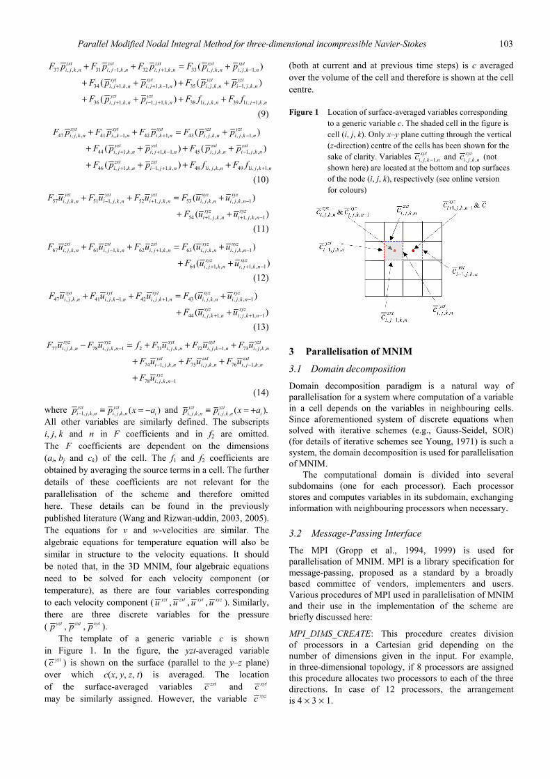
The template of a generic variable c is shown in Figure 1. In the figure, the yzt-averaged variable ( yztc ) is shown on the surface (parallel to the y–z plane) over which c(x, y, z, t) is averaged. The location of the surface-averaged variables zxtc and xytc may be similarly assigned. However, the variable xyzc

(both at current and at previous time steps) is c averaged over the volume of the cell and therefore is shown at the cell centre.

Figure 1 Location of surface-averaged variables corresponding to a generic variable c. The shaded cell in the figure is cell (i, j, k). Only x–y plane cutting through the vertical (z-direction) centre of the cells has been shown for the sake of clarity. Variables , , 1,

xyti j k nc − and , , ,

xyti j k nc (not

shown here) are located at the bottom and top surfaces of the node (i, j, k), respectively (see online version for colours)

3 Parallelisation of MNIM

3.1 Domain decomposition

Domain decomposition paradigm is a natural way of parallelisation for a system where computation of a variable in a cell depends on the variables in neighbouring cells. Since aforementioned system of discrete equations when solved with iterative schemes (e.g., Gauss-Seidel, SOR) (for details of iterative schemes see Young, 1971) is such a system, the domain decomposition is used for parallelisation of MNIM.

The computational domain is divided into several subdomains (one for each processor). Each processor stores and computes variables in its subdomain, exchanging information with neighbouring processors when necessary.

3.2 Message-Passing Interface

The MPI (Gropp et al., 1994, 1999) is used for parallelisation of MNIM. MPI is a library specification for message-passing, proposed as a standard by a broadly based committee of vendors, implementers and users. Various procedures of MPI used in parallelisation of MNIM and their use in the implementation of the scheme are briefly discussed here:

MPI_DIMS_CREATE: This procedure creates division of processors in a Cartesian grid depending on the number of dimensions given in the input. For example, in three-dimensional topology, if 8 processors are assigned this procedure allocates two processors to each of the three directions. In case of 12 processors, the arrangement is 4 × 3 × 1.

104 S. Singh and Rizwan-uddin

MPI_CART_CREATE: This procedure creates a new communicator with Cartesian topology based on the output of MPI_DIMS_CREATE. Each processor is assigned a coordinate according to its position in a virtual three-dimensional array of the processors.

MPI_CART_SHIFT: The procedure is used to identify immediate neighbouring processors in all the directions. The procedure needs to be called once for each direction to assign neighbours in that direction. For periodic topology, the procedure identifies the neighbours suitably. The input argument of this procedure contains a logical array variable of size three to identify the directions in which the topology is periodic.

MPI_BCAST: The input data is read by one of the processors and broadcasted to all the processors using this procedure. Before broadcasting, the input data is stored in two arrays, one for integer variables and for double precision variables. Only two calls of the procedure, one for each array, are then required to broadcast the data. Two arrays are required, as two different datatypes cannot be communicated simultaneously. The values of various parameters are then assigned from those processors in each array.

It is pointed out here that one array can also be used to broadcast the input variables by using a derived datatype, which consists of both datatypes. However, the broadcast is required only once and hence it is obviously not very useful to define a new datatype for the purpose.

Once the total number of cells is known to a processor, the starting and end cell numbers in each direction in that processor is evaluated depending on its position in the three-dimensional array assigned by MPI_CART_ CREATE. This is done so as to keep the computational load evenly balanced among the processors.

MPI_SEND_RECV: During the iterative process, the required communications, as discussed in the previous section, are carried out using this procedure.

MPI_ALL_REDUCE: Each processor checks convergence after each Gauss-Seidel iteration only locally. Global convergence is checked by using this procedure.

3.3 Communication between processors

The discrete variables that must be communicated to neighbouring processors depend on the ‘template’ in the set of algebraic equations. The variables thus communicated are stored in the ghost surfaces or cells in the receiving processor. Figure 2 shows two neighbouring subdomains in the x-direction. The figure is in the x–y plane showing only one layer of cells. All layers of cells in the z-direction will follow the same communication procedure.

From Equations (11) and (14), it can be seen that the variable yztu for the cells at the interface of two processors (corresponding to two subdomains) next to each other in the x-direction needs to be exchanged between them.

In Figure 3, the surfaces shown in the red colour (solid line) on the left processor are the ghost surfaces, which receive

yztu variable computed at the red surfaces in the right processor. This communication is shown by the red (solid line) arrow. The green colour surfaces and green (dashed line) arrow represent similar communication in the opposite direction. Similar communications are required for the variables zxtu and xytu between the processors next to each other in the y- and z-directions, respectively.

Figure 2 Decomposition of computational domain into eight subdomains

Figure 3 Communications required for the velocity equations in the x-direction (see online version for colours)

In addition, xyzu from the cells at the interface is communicated from each processor to its neighbouring processor in the negative x-direction. Since xyzu are node-averaged velocities, ghost cells (shaded cells in Fig. 3) are created to store the variable. The blue dots and blue (dotted line) arrow in the figure represent the above-mentioned communication. Similar communications are required in the y- and z-directions as well. The communications for corresponding variables in v, w and temperature equations are similar to those for the u equation.

Figure 4, which is similar to Figure 3, shows the communications of pressure variables between neighbouring processors in the x-direction. For pressure field, from Equation (8), it can be seen that yztp needs to be exchanged between the neighbouring processors in the x-direction. This communication is shown by red (solid line) and green (dashed line) colour arrows in Figure 4. Similar communications of corresponding variables are also needed in the y- and z-directions.

Also, ,xytp zxtp and f1 from the cells adjacent to the interface are communicated from each processor to its neighbouring processor in the negative x-direction. The communications for zxtp and f1 are shown in brown (dash-dot line) and blue (dotted line) colours, respectively. The communication for xytp is not shown in the figure for sake of clarity. Similar communications are also required in the y- and z-directions. All these communications are ideally needed at each iteration.

Parallel Modified Nodal Integral Method for three-dimensional incompressible Navier-Stokes 105

Figure 4 Communications required for the pressure equations in the x-direction (see online version for colours)

Special care is needed for communication of pressure variables in the corner cells. Figure 5 shows the communication of zxtp variable in the corner cell from where it is communicated to its destination. The above-mentioned variable is communicated to the neighbour in the diagonal direction. This process is carried out in two steps. First, the variable moves to the neighbour in the positive y-direction. From the receiving processor, this variable is moved to its neighbour to the left. Therefore, it is important to note that the communication shown by the red arrow (solid line) in the figure must precede the communication shown by the green arrow (dashed line). Otherwise, upper left processor in Figure 5 will not have the correct value. Similar care in the order of communications is also required for xytp and yztp variables in the corner cells.

Figure 5 Order of communication for the pressure variables in corner cell surfaces. Communication shown by solid arrow must precede that shown by dashed arrow (see online version for colours)

The coefficients in Equations (11)–(14) depend, in addition to the cell dimensions, on the previous time step velocities from that cell and the neighbouring cells. Therefore, ,pu pv and pw are also sent to neighbouring cells in the negative x-, y- and z-directions, respectively, but only once at each time step.

3.4 Communication cost relative to computational cost

The efficiency of parallel computation depends on efforts spent on communication between the processors relative to

computations carried out in each processor. The efficiency is higher if the cost of the communication is less.

For a Gauss-Seidel solver, the computational cost per cell for MNIM is approximately four times that for finite volume method because there are four surface-averaged variables for each velocity component (The advantage of the MNIM results from the fact that number of grid points, or cells, required is significantly less than that required for finite volume method for the same level of accuracy (Wang and Rizwan-uddin, 2003)). However, there are only two variables corresponding to each velocity component, which need to be communicated between the processors. Therefore, in MNIM, only half of the variables that are computed need to be communicated as opposed to all the variables in the case of finite volume method. Hence, it can be a priori concluded that parallelisation of MNIM is more likely to be more efficient than that for finite volume method. However, pressure equations need communications of four variables ( ,yztp ,zxtp xytp and f1) in each direction leading to no advantage over finite difference or finite volume parallelisation schemes. Since there are three velocity components and obviously only one pressure, overall parallelisation efficiency of PMNIM is expected to be higher than that for finite difference or control volume schemes.

In the above-mentioned discussion, the communication cost of previous time step velocities has been ignored, as they are sent only once for each time step. This cost is assumed to be negligible compared with the communication cost of variables that must be transmitted at each iteration.

4 Numerical results

4.1 Comparison with Benchmark solution

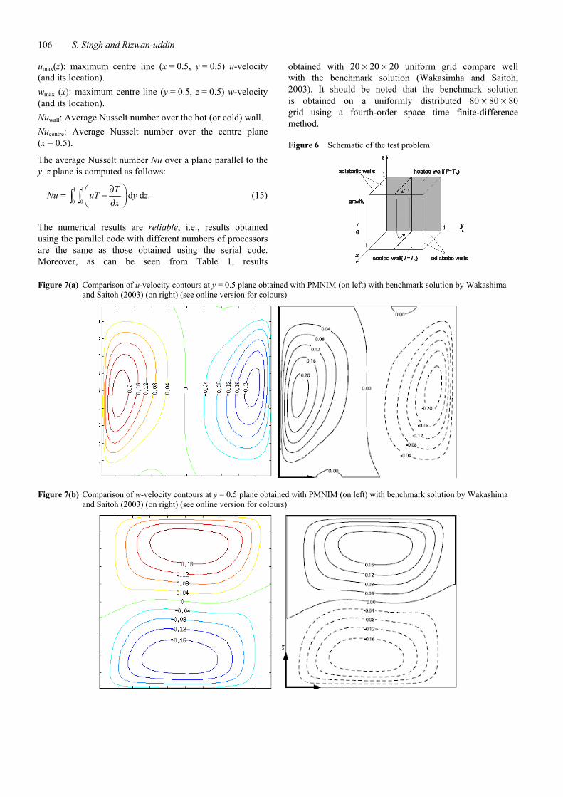
The PMNIM is used to simulate natural convection in a three-dimensional cubic cavity of unit dimensions. The schematic diagram of the problem is shown in Figure 6. The fluid in the cavity is air (Prandtl number 0.71), and Rayleigh number is 104. Gravity is in the z-direction. All surrounding walls are rigid and impermeable. The wall at x = 0 and x = 1 are isothermal but at different temperatures of Th and Tc, respectively. The remaining four walls are adiabatic. The flow is assumed to be incompressible and laminar. The Boussinesq approximation has been assumed to be valid. The equations are solved in the primitive variables. Simulations are carried out on the Turing cluster, which consists of 640 Apple Xserves, each with two 2 GHz G5 processors. The primary network connecting the cluster machines is a high-bandwidth, low-latency Myrinet network.

Figure 7 shows the velocity and temperature profiles at y = 0.5 plane for the test problem. The u and w velocity contours (a, b) and isotherms (c) are shown in the figure. The following quantities obtained using the PMNIM are compared in Table 1 with those reported for the benchmark solution given by Wakashima and Saitoh (2003).

106 S. Singh and Rizwan-uddin

umax(z): maximum centre line (x = 0.5, y = 0.5) u-velocity (and its location). wmax (x): maximum centre line (y = 0.5, z = 0.5) w-velocity (and its location). Nuwall: Average Nusselt number over the hot (or cold) wall. Nucentre: Average Nusselt number over the centre plane (x = 0.5).

The average Nusselt number Nu over a plane parallel to the y–z plane is computed as follows:

1 1

0 0d d .TNu uT y z

x∂ = − ∂ ∫ ∫ (15)

The numerical results are reliable, i.e., results obtained using the parallel code with different numbers of processors are the same as those obtained using the serial code. Moreover, as can be seen from Table 1, results

obtained with 20 × 20 × 20 uniform grid compare well with the benchmark solution (Wakasimha and Saitoh, 2003). It should be noted that the benchmark solution is obtained on a uniformly distributed 80 × 80 × 80 grid using a fourth-order space time finite-difference method.

Figure 6 Schematic of the test problem

Figure 7(a) Comparison of u-velocity contours at y = 0.5 plane obtained with PMNIM (on left) with benchmark solution by Wakashima and Saitoh (2003) (on right) (see online version for colours)

Figure 7(b) Comparison of w-velocity contours at y = 0.5 plane obtained with PMNIM (on left) with benchmark solution by Wakashima and Saitoh (2003) (on right) (see online version for colours)

Parallel Modified Nodal Integral Method for three-dimensional incompressible Navier-Stokes 107

Figure 7(c) Comparison of temperature contours at y = 0.5 plane obtained with PMNIM (on left) with benchmark solution by Wakashima and Saitoh (2003) (on right) (see online version for colours)

Table 1 Comparison of some of the results obtained using the

PMNIM with the benchmark solution

PMNIM Benchmark

umax (z) 0.1995 (0.826) 0.1984 (0.825) wmax (x) 0.2217 (0.117) 0.2216 (0.117) Nuwall 2.0621 2.0634 Nucentre 2.0751 2.0636

Source: Wakashima and Saitoh (2003)

4.2 Efficiency with fixed problem size per processor

It is now well established that the parallelisation efficiency is best measured by increasing the problem size as the number of processors is increased (Gustafson, 1988, 1990). Therefore, parallelisation performance is evaluated in this section by keeping the problem size for each processor fixed. To achieve this goal, the number of grid points or cells in each processor is kept constant while number of processors is increased. However, as the total number of grid points or cells changes in this case, number of iterations to converge will also change. Therefore, number of iterations is also kept fixed so as to achieve the above-mentioned objective.

Since problem size per processor is fixed, therefore it is expected that the running time, in the absence of communication cost, should remain constant irrespective of the number of processors. In view of the above-mentioned statement, speedup S for fixed problem size is defined as,

s

p

pTS

T= (16)

and efficiency E is defined as

s

p

TE

T= (17)

where p is the number of processors, Ts is runtime when a single processor is used and Tp is runtime when p number of processors are used.

The speedups and efficiency for a 10 × 10 × 10 grid in each processor are given in Table 2. The number of iterations performed is 5000. The computations take into account not only the effect of the number of processors but also the effect of processor configurations as well.

Table 2 Speedup and efficiency with 10 × 10 × 10 grid for each processor for fixed problem size per processor

Processor configuration Time (s) Speedup Efficiency (%)

1 × 1 × 1 72.52 1 100

2 × 1 × 1 78.22 1.85 92.70

3 × 1 × 1 80.97 2.69 89.56

4 × 1 × 1 81.84 3.54 88.61

2 × 2 × 1 86.70 3.35 83.65

3 × 2 × 1 87.61 4.97 82.77

2 × 2 × 2 93.88 6.18 77.24

3 × 3 × 1 91.90 7.20 80.01

4 × 3 × 1 93.80 9.28 77.32

3 × 2 × 2 94.80 9.18 76.50

4 × 4 × 1 95.66 12.13 75.81

4 × 2 × 2 97.79 11.86 74.16

3 × 3 × 3 102.31 19.14 70.88

4 × 3 × 3 103.06 25.33 70.37

5 × 3 × 3 104.31 31.29 69.52

4 × 4 × 3 104.54 33.29 69.37

4 × 4 × 4 105.91 43.82 68.47

It is obvious that the efficiency of a given configuration depends on the processor with maximum number of neighbours. Moreover, if the highest number of neighbours

108 S. Singh and Rizwan-uddin

in different configurations is the same, efficiencies are similar even if total number of processors is significantly different. For example, efficiency for 3 × 3 × 3 configuration is almost the same as that for 4 × 4 × 4 configuration because processor with maximum number of neighbours has six neighbours in both cases. The small decrease in efficiency can be attributed to the fact that the communication cost associated with the convergence check depends only on the total number of processors and not on the number of grid points. Since the maximum number of neighbours will not exceed six, therefore, the efficiency approaches a (nearly) constant value as the number of processors is increased. In other words, scalability of the scheme is quite good.

It can be seen that efficiency not only depends on the number of processors but also on the configuration of the processors, i.e., the efficiency for the same number of processors is different for different processor configurations. Such a trend is expected since blocking communication MPI_SEND_RECV is used in the implementation of the scheme. The blocking communication makes all the processors to wait for the exchange of one set of variables (initiated by the first MPI_SEND_RECV) before initiating the communication for the subsequent MPI_SEND_RECV. This can be further explained by considering the case of 2 × 2 × 1 configuration and comparing it with the case of 4 × 1 × 1. In 2 × 2 × 1 configuration, each processor has to communicate with two neighbouring processors in different directions. Although some processors in 4 × 1 × 1 configuration do have to communicate with two processors, the communication is only in the x-direction. Since MPI_SEND_RECV simultaneously communicates all information in one direction (say, x) and only then starts communicating in the other directions, the result is that the efficiency of 4 × 1 × 1 configuration is higher among the two cases considered here. Moreover, 4 × 1 × 1 and 3 × 1 × 1 configuration efficiencies are not significantly different. Figure 8 shows the speedup for the cases in which at least one processor has six neighbours.

The efficiencies with different numbers of processors for the 20 × 20 × 20 grid (for 5000 iterations) are given in Table 3. The trends observed for the 20 × 20 × 20 grid case are similar to those for the 10 × 10 × 10 grid. The ratio of cells at the interface to total number of cells decreases as total number of grid points is increased. Therefore, in general, efficiency of 20 × 20 × 20 case should be higher than 10 × 10 × 10 grid. However, this is true only if communication cost of sending data is independent of the size of the data. This assumption is usually not valid because of limitations of the bus size used for data exchange. For the 3D thermal cavity problem solved using the PMNIM, however, the efficiency of the 20 × 20 × 20 case for some configurations is lower than the 10 × 10 × 10 grid case while it is higher for other configurations. The result may be explained by the fact that contiguity of data to be sent in different directions is not the same. This result in higher

communication cost in the direction in which communicated data is non-contiguous. Figure 9 shows the speedup for the cases in which at least one processor has six neighbours.

Figure 8 Speedup of PMNIM with 10 × 10 × 10 grid for fixed problem size per processor. All cases shown here have at least one processor with six neighbours. Efficiency ranges from 68.47% to 70.88%

Figure 9 Speedup of PMNIM with 20 × 20 × 20 grid for fixed problem size per processor. All cases shown here have at least one processor with six neighbours. Efficiency ranges from 75.58% to 78.02%

Table 3 Speedup and efficiency with 20 × 20 × 20 grid for each processor for fixed problem size per processor (continues on next page)

Processor configuration Time (s) Speedup Efficiency (%)

1 × 1 × 1 2542.66 1 100

2 × 1 × 1 2846.66 1.79 89.32

3 × 1 × 1 2877.33 2.65 88.36

4 × 1 × 1 2899.66 3.50 87.68

2 × 2 × 1 2900.33 3.47 87.66

3 × 2 × 1 2900.66 5.26 87.65

2 × 2 × 2 3050.33 6.67 83.35

3 × 3 × 1 2967.01 7.71 85.69

4 × 3 × 1 2985.33 10.22 85.17

Parallel Modified Nodal Integral Method for three-dimensional incompressible Navier-Stokes 109

Table 3 Speedup and efficiency with 20 × 20 × 20 grid for each processor for fixed problem size per processor (continued)

Processor configuration Time (s) Speedup Efficiency (%)

3 × 2 × 2 3000.66 10.09 84.05

4 × 4 × 1 3025.00 13.55 84.73

4 × 2 × 2 3038.66 13.39 83.67

3 × 3 × 3 3291.05 20.86 77.26

4 × 3 × 3 3258.66 28.09 78.02

5 × 3 × 3 3364.03 34.01 75.58

4 × 4 × 3 3346.02 36.47 75.99

4 × 4 × 4 3300.05 49.31 76.05

4.3 Efficiency with variable problem size per processor

In this subsection, whereas the problem size per processor is varied, the overall problem size is kept fixed, i.e., the total number of cells is kept constant. The problem size per processor, therefore, decreases as number of processors increases. The number of iterations remains almost same irrespective of the number of processors used. The definition of speedup, S, relevant for this subsection, for a given number of processors, is as follows:

.s

p

TS

T= (18)

The efficiency E is defined as:

.s

p

TE

pT= (19)

The performance is evaluated for two cases with 12 × 12 × 12 and 20 × 20 × 20 grid. Speedup and efficiency for PMNIM with 12 × 12 × 12 grid are presented in Table 4. Figure 10 shows the plot for the speedup for 12 × 12 × 12 grid case. It can be seen that as the number of processors is increased the speedup and efficiency decrease. This expected behaviour is observed because, for a given grid, the communication cost goes up with the number of processors while computation cost remains unchanged. It can be seen from Table 4 that the drop in efficiency is rapid for relatively higher number of processors. This rapid drop is because that a small number of cells are being distributed over a large number of processors resulting in large number of cells at interfaces, which need communication of variables, thereby increasing the communication cost relative to the computation cost. For example, with 24 processors number of cells in each processor is 72 while number of cells at interfaces is 96, leading to reduced efficiency.

Figure 10 Speedup of PMNIM with 12 × 12 × 12 grid for variable problem size per processor

Table 4 Speedup and efficiency with 12 × 12 × 12 grid, for variable problem size per processor

Processors Time (m) Speedup Efficiency (%)

24 2.77 6.42 26.8 16 2.90 6.13 38.3 12 2.92 6.09 50.7 8 3.43 5.17 64.6 6 3.65 4.87 81.2 4 4.78 3.71 92.8 2 9.03 1.97 98.6 1 17.78 1 100.0

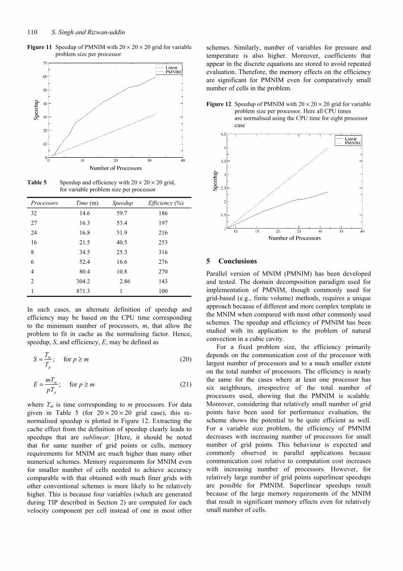
Table 5 presents the speedup and efficiency of PMNIM with 20 × 20 × 20 grid. Figure 11 shows plot for the speedup for 20 × 20 × 20 grid case. The efficiency and speedup trends for this case are very different from the 12 × 12 × 12 grid case. The efficiency increases with increasing number of processors initially and only then starts to decrease. Moreover, efficiency is greater than 100%. Superlinear efficiencies have been encountered in the past and they are associated with memory/cache effects (Gustafson, 1990; Helmbold and McDowell, 1989; Parkinson, 1986). Therefore, it is possible that for a relatively large problem, the memory required exceeds the size of the faster memory type (cache) if small number of processors is used. This results in increase in efficiency with number of processors because a larger fraction of the memory need is satisfied by the faster memory type as the number of processors is increased (Gustafson, 1990; Helmbold and McDowell, 1989; Parkinson, 1986). The efficiency starts decreasing only when the communication cost starts dominating over the memory effect. CPU times for different numbers of processors in Table 5 suggest that a qualitatively different kind of change takes place as the number of processors is changed from 6 to 8, suggesting that for given capabilities of the processors used and the problem size (20 × 20 × 20), minimum of 8 processors are needed to satisfy the memory requirement entirely by the faster memory.

110 S. Singh and Rizwan-uddin

Figure 11 Speedup of PMNIM with 20 × 20 × 20 grid for variable problem size per processor

Table 5 Speedup and efficiency with 20 × 20 × 20 grid, for variable problem size per processor

Processors Time (m) Speedup Efficiency (%)

32 14.6 59.7 186 27 16.3 53.4 197 24 16.8 51.9 216 16 21.5 40.5 253 8 34.5 25.3 316 6 52.4 16.6 276 4 80.4 10.8 270 2 304.2 2.86 143 1 871.3 1 100

In such cases, an alternate definition of speedup and efficiency may be based on the CPU time corresponding to the minimum number of processors, m, that allow the problem to fit in cache as the normalising factor. Hence, speedup, S, and efficiency, E, may be defined as

; form

p

TS p m

T= ≥ (20)

; form

p

mTE p m

pT= ≥ (21)

where Tm is time corresponding to m processors. For data given in Table 5 (for 20 × 20 × 20 grid case), this re-normalised speedup is plotted in Figure 12. Extracting the cache effect from the definition of speedup clearly leads to speedups that are sublinear. [Here, it should be noted that for same number of grid points or cells, memory requirements for MNIM are much higher than many other numerical schemes. Memory requirements for MNIM even for smaller number of cells needed to achieve accuracy comparable with that obtained with much finer grids with other conventional schemes is more likely to be relatively higher. This is because four variables (which are generated during TIP described in Section 2) are computed for each velocity component per cell instead of one in most other

schemes. Similarly, number of variables for pressure and temperature is also higher. Moreover, coefficients that appear in the discrete equations are stored to avoid repeated evaluation. Therefore, the memory effects on the efficiency are significant for PMNIM even for comparatively small number of cells in the problem.

Figure 12 Speedup of PMNIM with 20 × 20 × 20 grid for variable problem size per processor. Here all CPU times are normalised using the CPU time for eight processor case

5 Conclusions

Parallel version of MNIM (PMNIM) has been developed and tested. The domain decomposition paradigm used for implementation of PMNIM, though commonly used for grid-based (e.g., finite volume) methods, requires a unique approach because of different and more complex template in the MNIM when compared with most other commonly used schemes. The speedup and efficiency of PMNIM has been studied with its application to the problem of natural convection in a cubic cavity.

For a fixed problem size, the efficiency primarily depends on the communication cost of the processor with largest number of processors and to a much smaller extent on the total number of processors. The efficiency is nearly the same for the cases where at least one processor has six neighbours, irrespective of the total number of processors used, showing that the PMNIM is scalable. Moreover, considering that relatively small number of grid points have been used for performance evaluation, the scheme shows the potential to be quite efficient as well. For a variable size problem, the efficiency of PMNIM decreases with increasing number of processors for small number of grid points. This behaviour is expected and commonly observed in parallel applications because communication cost relative to computation cost increases with increasing number of processors. However, for relatively large number of grid points superlinear speedups are possible for PMNIM. Superlinear speedups result because of the large memory requirements of the MNIM that result in significant memory effects even for relatively small number of cells.

Parallel Modified Nodal Integral Method for three-dimensional incompressible Navier-Stokes 111

Acknowledgements

This research was supported in part by an INIE grant from the US Department of Energy. The authors also acknowledge use of the Turing cluster, which is operated by the Computational Science and Engineering Programme at the University of Illinois.

References Azmy, Y.Y. (1985) Nodal Method for Problems in Fluid

Mechanics and Neutron Transport, PhD Thesis, University of Illinois, Urbana, Illinois.

Azmy, Y.Y. and Dorning, J.J. (1983) ‘A nodal integral approach to the numerical solution of partial differential equations’, Proceedings of Advances in Reactor Computations, Salt Lake City, UT, 28–30 March, Vol. II, pp.893–909.

Basu, A.J. (1994) ‘A parallel algorithm for spectral solution of the three-dimensional Navier-Stokes equations’, Parallel Comput., Vol. 20, No. 8, pp.1191–1204.

Chen, S. and Shan, X. (1992) ‘High-resolution turbulent simulations using the connection machine-2’, Comput. Phys., Vol. 6, No. 6, pp.643–646.

Elnawawy, O.A., Valocchi, A.J. and Ougouag, A.M. (1990) ‘The cell analytical-numerical method for solution of the advection-dispersion equation: two-dimensional problems’, Water. Resour. Res., Vol. 26, No. 11, pp.2705–2716.

Esser, P.D. and Witt, R.J. (1993) ‘An upwind nodal integral method for incompressible fluid flow’, Nucl. Sci. Engrg., Vol. 114, No. 1, pp.20–35.

Garg, R.P., Ferziger, J.H. and Monismith, S.G. (1997) ‘Hybrid spectral finite difference simulations of stratified turbulent flows on distributed memory architectures’, Int. J. Numer. Meth. Fluids, Vol. 24, No. 11, pp.1129–1158.

Gropp, W., Skjellum, A. and Lusk, E. (1994) Using MPI: Portable Parallel Programming with the Message-Passing Interface, MIT Press, Cambridge, MA.

Gropp, W., Skjellum, A. and Thakur, R. (1999) Using MPI-2: Advanced Features of the Message-Passing Interface, MIT Press, Cambridge, MA.

Gu, Y. and Rizwan-uddin (2005) ‘A hybrid method for multi-group neutron diffusion equations in arbitrary geometry’, Proceedings of International Topical Meeting on Mathematics and Computations, Supercomputing, Reactor Physics and Nuclear and Biological Applications (M&C), Avignon, France, 12–15 September, Available on CD-ROM.

Gustafson, J.L. (1988) ‘Reevaluating Amdahl’s law’, CACM, Vol. 31, No. 5, pp.532–533.

Gustafson, J.L. (1990) ‘Fixed time, tiered memory, and superlinear speedup’, Proceedings of Fifth Conference on Distributed Memory Computing (DMCC5), Charleston, SC, USA, 9–12 April, pp.1255–1260.

Helmbold, D.P. and McDowell, C.E. (1989) ‘Modeling Speedup(n) greater than n’, Proceedings of International Conference on Parallel Processing, University Park, PA, USA, 8–12 August, pp.219–225.

Hennart, J.P. (1986) ‘A general family of nodal schemes’, SIAM J. Sci. Stat. Comp., Vol. 7, No. 1, pp.264–287.

Horak, W.C. and Dorning, J.J. (1985) ‘A nodal coarse-mesh method for the efficient numerical solution of laminar flow problems’, J. Comp. Physics, Vol. 59, No. 3, pp.405–440.

Jackson, E., She, Z.S. and Orszag, S.A. (1991) ‘A case study in parallel computing: inhomogeneous turbulence on a hypercube’, J. Sci. Comput., Vol. 6, No. 1, pp.27–45.

Johan, Z. and Hughes, T.J.R. (1992) ‘A data parallel finite element method for computational fluid dynamics on the connection machine system’, Comput. Meth. Appl. Mech. Eng., Vol. 99, No. 1, pp.113–134.

Lawrence, R.D. (1986) ‘Progress in nodal methods for the solutions of the neutron diffusion and transport equations’, Progress in Nuclear Energy, Vol. 17, No. 3, pp.271–301.

Levit, C. and Jespersen, D. (1988) ‘Explicit and implicit solution of the Navier–Stokes equations on a massively parallel computer’, Comput. Struct., Vol. 30, Nos. 1–2, pp.385–393.

Liu, C.H., Leung, D.Y.C. and Woo, C.M. (2003) ‘Development of a scalable finite element solution to the Navier-Stokes equations’, Computational Mechanics, Vol. 32, No. 3, pp.185–198.

Michael, E.P.E., Dorning, J.J. and Rizwan-uddin (2001) ‘Studies on nodal integral methods for the convection–diffusion heat equation’, Nucl. Sci. Eng., Vol. 137, No. 3, pp.380–399.

Mittal, S. and Tezduyar, T.E. (1995) ‘Parallel finite element simulation of 3D incompressible flows: Fluid-structure interactions’, Int. J. Numer. Meth. Fluids, Vol. 21, No. 10, pp.933–953.

Naik, H., Naik, V.K. and Nicoules, M. (1993) ‘Parallelization of a class of implicit finite difference schemes in computational fluid dynamics’, Int. J. High Speed Comp., Vol. 5, No. 1, pp.1–50.

Nezami, E., Singh, S., Sobh, N. and Rizwan-uddin (2009) ‘A nodal integral method for quadrilateral elements’, Int. J. Numer. Meth. Fluids, Vol. 61, No. 2, pp.144–164.

Parkinson, D. (1986) ‘Parallel efficiency can be greater than unity’, Parallel Comput., Vol. 3, No. 3, pp.261–262.

Passoni, G., Cremonesi, P. and Alfonsi, G. (2001) ‘Analysis and implementation of a parallelization strategy on a Navier-Stokes solver for shear flow simulations’, Parallel Comput., Vol. 27, No. 13, pp.1665–1685.

Pelz, R.B. (1991) ‘The parallel Fourier pseudo-spectral method’, J. Comput. Phys., Vol. 92, No. 2, pp.296–312.

Peyret, R. (2002) Spectral Methods for Incompressible Viscous Flows, Springer, New York.

Prestin, M. and Shtilman, L. (1995) ‘A parallel Navier–Stokes solver: the Meiko implementation’ J. Supercomput., Vol. 9, No. 4, pp.347–364.

Toreja, A.J. and Rizwan-uddin (2003a) ‘A hybrid nodal method for time-dependent incompressible flow in two-dimensional arbitrary geometries’, Proceedings of Nuclear Mathematical and Computational Sciences: A Century in Review, A Century Anew (M&C), 6–10 April, Gatlinburg, TN, USA, Available on CD-ROM.

Toreja, A.J. and Rizwan-uddin (2003b) ‘Hybrid numerical methods for convection–diffusion problems in arbitrary geometries’, Computers and Fluids, Vol. 32, No. 6, pp.835–872.

Wakashima, S. and Saitoh, T.S. (2003) ‘Benchmark solutions for natural convection in a cubic cavity using the high order time-space method’, Int. J. Heat Mass Transfer, Vol. 47, No. 4, pp.853–864.

Wang, F. and Rizwan-uddin (2003) ‘A modified nodal scheme for the time-dependent, incompressible Navier-Stokes equations’, J. Comp. Physics, Vol. 187, No. 1, pp.168–196.

112 S. Singh and Rizwan-uddin

Wang, F. and Rizwan-uddin (2005) ‘Modified nodal integral method for the three-dimensional time-dependent incompressible Navier-Stokes equations’, Nucl. Sci. Engrg., Vol. 149, No. 1, pp.107–114.

Wasfy, T., West, A.C. and Modi, V. (1998) ‘Parallel finite element computation of unsteady incompressible flows’, Int. J. Numer. Meth. Fluids, Vol. 26, No. 1, pp.17–37.

Wescott, B. and Rizwan-uddin (2001) ‘An efficient formulation of the modified nodal integral method and application to the two dimensional Burgers equation’, Nucl. Sci. Engrg., Vol. 139, No. 1, pp.293–305.

Wilson, G.L., Rydin, R.A. and Azmy, Y.Y. (1988) ‘Time-dependent nodal integral method for the investigation of bifurcation and nonlinear phenomena in fluid flow and natural convection’, Nucl. Sci. Engrg., Vol. 100, No. 4, pp.414–425.

Wu, J., Ritzdorf, H., Oosterlee, K., Steckel, B. and Schüller, A. (1997) ‘Adaptive parallel multigrid solution of 2D incompressible Navier–Stokes equations’, Int. J. Numer. Meth. Fluids, Vol. 24, No. 9, pp.875–892.

Young, D. (1971) Iterative Solutions of Large Linear Systems, Academic Press, New York.