IEEE TRANSACTIONS ON IMAGE PROCESSING 1

A reliable order-statistics-basedapproximate nearest neighbor search algorithm

Luisa Verdoliva, Davide Cozzolino, Giovanni Poggi

Abstract—We propose a new algorithm for fast approximatenearest neighbor search based on the properties of orderedvectors. Data vectors are classified based on the index and signof their largest components, thereby partitioning the space ina number of cones centered in the origin. The query is itselfclassified, and the search starts from the selected cone andproceeds to neighboring ones. Overall, the proposed algorithmcorresponds to locality sensitive hashing in the space of directions,with hashing based on the order of components. Thanks tothe statistical features emerging through ordering, it deals verywell with the challenging case of unstructured data, and is avaluable building block for more complex techniques dealing withstructured data. Experiments on both simulated and real-worlddata prove the proposed algorithm to provide a state-of-the-artperformance.

Index Terms—Approximate nearest neighbor search, localitysensitive hashing, vector quantization, order statistics.

I. INTRODUCTION

A large number of applications in computer vision andimage processing need to retrieve, in a collection of vectors,the nearest neighbor (NN) to a given query. A well-knownexample is image retrieval based on compact descriptors, butthere are countless more, from patch-based image denoising,to copy-move forgery detection, data compression, and soon. Typically, large sets of points are involved, calling forfast search techniques to guarantee an acceptable processingtime. However, for high-dimensional data, no exact NN searchalgorithm can provide a significant speed-up w.r.t. linearsearch, so one is forced to settle for some approximate searchalgorithms, trading off accuracy for efficiency.

In recent years, there has been intense research on tech-niques that improve this trade-off. These can be classifiedin two large families according to their focus on memoryor time efficiency. A first family [1], [2], [3], [4] addressesthe case of very large datasets, that do not fit in memory.This may occur, for example, in image retrieval and othercomputer vision applications. In this condition, performing anaccurate search based on Euclidean vector distances wouldrequire data transfers from disk, with an exceedingly largedelay. By associating compact codes with original vectors, andapproximating exact distances based on such codes, one candrastically reduce memory usage and avoid buffering, with ahuge impact on search speed. In this case, therefore, memoryefficiency is the main issue and the prevailing measure ofperformance, while actual search time is of minor interest.

On the contrary, when data and associated structures canfit in memory, processing time becomes the main issue, and

Universita Federico II di Napoli – ITALY, e-mail name.surname@unina.it

performance is measured in terms of accuracy vs speed-up, with memory usage assuming minor importance. This isthe case of a large number of image processing application,especially in the patch-based paradigm. Notable examples arenonlocal denoising [5], exemplar-based inpainting [6], copy-move forgery detection [7] and optical flow estimation [8].The present work fits in the latter family. That is, our aim isto provide a large speed-up with respect to linear search whilestill guaranteeing a very high accuracy based on Euclideandistance computation on the original vectors.

Most techniques of this family follow a similar path, withmany variations: first the search space is partitioned intosuitable cells1, and all vectors are classified based on the cellthey belong to. Then, at run time, the query is itself classified,and the NN is searched only among vectors falling in the samecell as the query, or possibly in some neighboring ones. Statedin these terms, approximate NN (ANN) search bears strikingsimilarities with the vector quantization (VQ) problem [9],[10]. In both fields, defining a good partition of the space anda fast classification rule are the key ingredients of success.Hence similar concepts and tools are used [11].

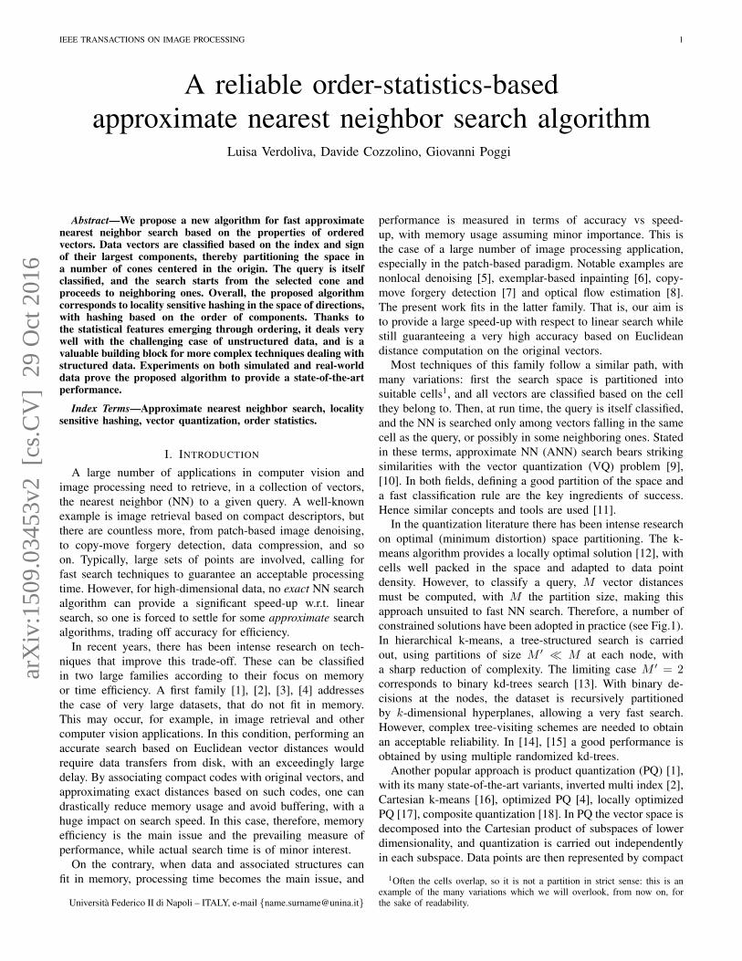
In the quantization literature there has been intense researchon optimal (minimum distortion) space partitioning. The k-means algorithm provides a locally optimal solution [12], withcells well packed in the space and adapted to data pointdensity. However, to classify a query, M vector distancesmust be computed, with M the partition size, making thisapproach unsuited to fast NN search. Therefore, a number ofconstrained solutions have been adopted in practice (see Fig.1).In hierarchical k-means, a tree-structured search is carriedout, using partitions of size M ′ M at each node, witha sharp reduction of complexity. The limiting case M ′ = 2corresponds to binary kd-trees search [13]. With binary de-cisions at the nodes, the dataset is recursively partitionedby k-dimensional hyperplanes, allowing a very fast search.However, complex tree-visiting schemes are needed to obtainan acceptable reliability. In [14], [15] a good performance isobtained by using multiple randomized kd-trees.

Another popular approach is product quantization (PQ) [1],with its many state-of-the-art variants, inverted multi index [2],Cartesian k-means [16], optimized PQ [4], locally optimizedPQ [17], composite quantization [18]. In PQ the vector space isdecomposed into the Cartesian product of subspaces of lowerdimensionality, and quantization is carried out independentlyin each subspace. Data points are then represented by compact

1Often the cells overlap, so it is not a partition in strict sense: this is anexample of the many variations which we will overlook, from now on, forthe sake of readability.

arX

iv:1

509.

0345

3v2

[cs

.CV

] 2

9 O

ct 2

016

IEEE TRANSACTIONS ON IMAGE PROCESSING 2

(a) (b) (c)

(d) (e) (f)

Fig. 1. ANN search is tightly related to quantization and space partitioning.Some important concepts may emerge even with a simple 2d example. Forstructured data, unconstrained vector quantization (a) is optimal but usuallytoo complex for real-world applications. Tree-structured VQ (b), and productVQ (c) reduce complexity but do not fully exploit data dependencies. Forunstructured data, it can make sense resorting to product scalar quantization(d). However, lattice VQ (e) provides a better tessellation of the space.Basic LSH corresponds to non-orthogonal product quantization (f), hence itis theoretically worse than both product and Lattice VQ.

codes obtained by stacking the quantization indices of allsubspaces. Thanks to these compact codes and to approxi-mate code-based distances, large datasets can be dealt withefficiently. The limiting case of scalar subspaces correspondsto the independent quantization of vector components. Thissolution is simple but largely suboptimal, and much betterregular partitions of the space can be found [19].

Interestingly, one of the most popular ANN search tech-niques, locality sensitive hashing (LSH) [20], [21], amountsto nothing more than scalar product quantization [11], withdata projected on randomly oriented, non-orthogonal, axes.Nonetheless, LSH can achieve a good performance througha number of clever expedients, like the use of multiple hashtables [20], and multi-probe search [22]. Moreover, data-dependent variants of LSH improve largely over basic LSH,by learning projection axes from the data [23], [24], [25], andusing non-uniform quantizers [11].

In general, taking advantage of the intrinsic structure of datacan greatly help speeding up the search. However, often datahave little or no structure, or become unstructured after somepreliminary processing. In hierarchical k-means, for example,as well in IVFADC [1], after the top-level quantization, thepoints become almost uniformly distributed in their cells.Looking for the NN when data have no structure is anespecially challenging task, encountered in many high-levelproblems, and therefore a fundamental issue of ANN search.

In this work we propose a Reliable Order-Statistics basedApproximate NN search Algorithm (ROSANNA) suited forunstructured data. Like in the methods described before,we define a suitable partition of the space, and carry outclassification and priority search. The main innovation consistsin classifying the data based just on the index and sign of theirlargest components. This simple pre-processing allows us topartition the search space effectively, with negligible complex-

ity and limited impact on memory usage. For each query, onlya short list of candidates is then selected for linear search.ROSANNA can be also regarded as a variant of LSH, wherethe hashing is based on the vector directions. This makesfull sense in high dimensions, since data tend to distributeon a spherical shell. ROSANNA produces a uniform partitionof the space of directions, and all vectors are automaticallyclassified based on the order of their sorted components. Byusing multiple hash tables, obtained through random rotationsof the basis, and a suitable visiting scheme of the cells, avery high accuracy is obtained, with significant speed-up w.r.t.reference techniques. Experiments on both unstructured andreal-world structured data prove ROSANNA to provide a state-of-the-art search performance. We also used ROSANNA toinitialize the NN field in copy-move forgery detection, a real-world computation-intensive image processing task, obtaininga significant speed-up.

In the vast literature on ANN search, several papers re-lated with ROSANNA have obviously appeared. For example,sorting has been already exploited by Chavez et al. [26].This technique, however, is pivot-based rather than partition-based. A number of anchor vectors, or “pivots” are chosen inadvance. Then, for each database vector the distances to allpivots are computed and sorted, keeping track of the orderin a permutation vector. At search time, a permutation vectoris computed also for the query and compared with those ofthe database points to select a short list of candidate NNs,assuming that close vectors have similar permutation vectors.In summary, sorting is used for very different goals than inthe proposed method.

If ROSANNA is regarded as LSH in the space of directions,then the same goal is pursued by the Spherical LSH (SLSH)proposed in [27], (not to be confused with the unrelatedSpherical Hashing [28]), where a regular Voronoi partitionof the unit hypersphere is built based on the vertices of aninscribed polytope. For example, working in a 3d space, theunit sphere can be partitioned in 8 cells corresponding tothe 8 vertices of the inscribed cube. Therefore, in SLSH, aregular partition is obtained with a low-complexity hashingrule [27]. Unfortunately, in high-dimensional spaces (K ≥ 5)there are only three kinds of regular polytopes, simplex, withK+1 vertices, orthoplex, with 2K vertices, and hypercubewith 2K vertices. SLSH uses eventually only the orthoplexpolytope, which corresponds to a strongly constrained versionof ROSANNA. Likewise, Iterative quantization (ITQ), pro-posed in [3] for ANN search through compact codes, makesreference to hyper-octants, and hence corresponds to another(opposite) constrained version of ROSANNA. By removingsuch constraints, ROSANNA is able to provide much betterresults.

In Concomitant LSH [29], instead, a Voronoi partition of thespace of directions is built based on a set of M points taken atrandom on the unit sphere. Although originally proposed forcosine distance, it presents some similarities with ROSANNA,the use of directions and sorting, and can be easily adaptedto deal with the Euclidean distance. However, to classify thequery, M distances must be computed at search-time, beforeinspecting the candidates, which is a severe overhead for

IEEE TRANSACTIONS ON IMAGE PROCESSING 3

p c x1 x2 x3

1

0 -22 12 5-21 -19 -12

1

29 24 -1344 17 -449 -6 557 8 -2

2

0 -3 -18 10-1 -13 0

15 11 4

11 14 -314 25 23

30

-36 23 -475 26 -279 -2 -17

12 5 -141 -7 11 22

p c x1 x2 x3

1-2

0 -21 -19 -12-1 -13 0

1 -22 12 52 49 -6 5

3

5 11 411 14 -329 24 -1344 17 -457 8 -2

1-3

0 -36 23 -47

2 9 -2 -1712 5 -14

2-3

1 -3 -18 102 5 26 -27

3 14 25 23-7 11 22

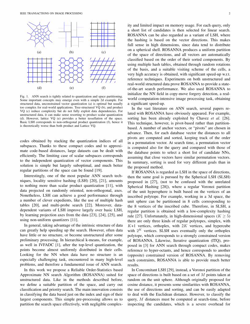
Fig. 2. Two different organization of the same dataset. Left: only the largestcomponent is used for classification, G=1. Profile p=1 includes all vectorswhere the first component, x1, is largest. The profile is divided in two cones,c=0, including vectors with x1 < 0, and c=1, including the others. Right:the two largest components are used for classification, G=2. Profile p=1-2 includes all vectors where x1 and x2 are the largest components. Theprofile is divided in four cones, according to the sign of these components.The largest G components are shown in bold and color.

large hashing tables. To reduce this burden, several variantsare also proposed in [29] which, however, tend to produce aworse partition of the space. Irrespective of the implementationdetails, the regular partition of the space of directions providedby ROSANNA can be expected to be more effective thanthe random partition used in Concomitant LSH. Moreover, inROSANNA, the hashing requires only a vector sorting, withno distance computation. As for concomitants (related to orderstatistics) they are only used to carry out a theoretical analysisof performance, but are not considered in the algorithm.

Recently, Cherian et al. proposed to use sparse ANN codes[30], where each data point is represented as a sparse combi-nation of unit-norm vectors drawn from a suitable dictionary.The indexes of the selected dictionary vectors represent a shortcode used to speed up retrieval. If a low-coherence dictionaryis designed [31], close data points tend to fall in the samebucket, a cone identified by the selected dictionary vectors,which is then searched linearly. This technique (SpANN) isexplicitly designed to deal with datasets with large nominaland low intrinsic dimensionality (i.e., sparse). Therefore, itis ineffective with unstructured data. In this case, the extraefforts of designing a low-coherence dictionary (off-line), andfinding the sparse code of the query (at search time) arebasically useless. ROSANNA can be seen as the limitingcase of SpANN when the vocabulary vectors are uniformlydistributed over the space of directions and a single vector isused to approximate a data point.

In the following, we first describe the basic algorithm andexplain its rationale (Section 2), then describe the full-fledgedimplementation (Section 3), discuss experiments on simulatedand real-world data (Section 4) and finally draw conclusions.

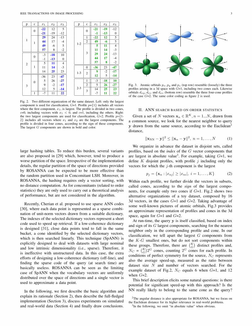
Fig. 3. Atomic orbitals px, py and pz (top row) resemble (loosely) the threeprofiles arising in a 3d space with G=1, including two cones each. Likewiseorbitals dxy , dxz and dxz (bottom row) resemble the three four-cone profilesof the case G=2. The same color coding as figure 2 is used.

II. ANN SEARCH BASED ON ORDER STATISTICS

Given a set of N vectors xn ∈ RK , n = 1...N , drawn froma common source, we look for the nearest neighbor to queryy drawn from the same source, according to the Euclidean2

distance,

‖xNN − y‖2 ≤ ‖xn − y‖2, n = 1, . . . , N (1)

We organize in advance the dataset in disjoint sets, calledprofiles, based on the index of the G vector components thatare largest in absolute value3. For example, taking G=1, wedefine K disjoint profiles, with profile j including only thevectors for which the j-th component is the largest

pj = xn : |xnj | ≥ |xni|, i = 1, . . . ,K (2)

Within each profile, we further divide the vectors in subsets,called cones, according to the sign of the largest compo-nents, for example only two cones if G=1. Fig.2 shows twoalternative organizations of a toy dataset, composed by 163d vectors, in the cases G=1 and G=2. Taking advantage ofsome well-known pictures of atomic orbitals, Fig.3 providesan approximate representation of profiles and cones in the 3dspace, again for G=1 and G=2.

At run-time, the query y is itself classified, based on indexand sign of its G largest components, searching for the nearestneighbor only in the corresponding profile and cone. In ourclassification, we tell apart the largest G components fromthe K-G smallest ones, but do not sort components withinthese groups. Therefore, there are

(KG

)distinct profiles and,

NC =(KG

)2G cones, counting 2G cones for each profile. In

conditions of perfect symmetry for the source, NC representsalso the average speed-up, measured as the ratio betweendataset size N and number of vectors searched. For theexample dataset of Fig.2, NC equals 6 when G=1, and 12when G=2.

This brief description elicits some natural questions: is therepotential for significant speed-up with this approach? Is theNN really likely to belong to the same cone as the query?

2The angular distance is also appropriate for ROSANNA, but we focus onthe Euclidean distance for its higher relevance in real-world problems.

3In the following, we omit “in absolute value” when obvious.

IEEE TRANSACTIONS ON IMAGE PROCESSING 4

−2 −1 0 1 2 3−3

−2

−1

0

1

2

3

−2 −1 0 1 2 3−3

−2

−1

0

1

2

3

Fig. 4. Scatter plots of the first two components of 512 8d Gaussian vectors.Left: randomly selected vectors. Right: vectors where the first two componentsare the largest ones.

Both questions may have a positive answer when we move tohigh-dimensional spaces, K 1, thanks to the properties oforder statistics.

Concerning speed-up, it is important to note that the numberof cones grows very quickly with K and G. For example,it is almost 30000 for K=16 and G=4. Note that K=16 isconsidered a relatively small dimensionality for NN searchproblems. By increasing the number of cones, one can reduceat will the average number of vectors per cone, hence thesearch time. Needless to say, in doing so, one should alwaysguarantee a high probability that the NN is actually found inthe searched cone (or cones).

To analyze this point, let us focus on the specific caseof vector components modeled as independent identicallydistributed (i.i.d.) random variables with standard Gaussiandistribution, Xi ∼ N (0, 1). This is arguably a worst case forthe NN search problem, as there is no structure in the data totake advantage of. It can be appreciated, for example, in theleft scatter plot of Fig.4, showing the first two componentsof 512 8-dimensional vectors with i.i.d. standard Gaussiancomponents. In the same plot we also show, in red, the firsttwo components of a query drawn from the same distribution.Clearly, there is not much structure in the data to help speedingup the NN search. The right scatter plot of Fig.4 is obtainedas the left one, except that we now include only vectors suchthat the first two components are also the largest ones. Thedifference between the two scatter plots is striking: sorting thecomponents has created a structure in the data, which can beexploited to speed-up the search. In particular, we can safelyrestrict attention to only one of the four emerging clusters (ourcones), comprising vectors where the sign of the two largestcomponents is the same as in the query, gaining therefore afactor four in speed. Still, it is not impossible that the trueNN belongs to a different cluster (it depends on the remainingcomponents) but there is an energy gap to overcome, due tothe query-cluster distance in the first two components.

Of course, after sorting, the components are not identicallydistributed anymore, and certainly not independent on oneanother. Given the probability density function (pdf) of theoriginal components, fX(x), we can easily compute the pdf ofthe sorted components. Let Ai = |Xi| be the absolute value ofthe i-th component, and A(i) the i-th component of the sortedvector of absolute values, such that A(i) ≥ A(i+1). Note that

−2 0 20

0.5

1

1.5

−2 0 20

0.5

1

1.5

−2 0 20

0.5

1

1.5

−2 0 20

0.5

1

1.5

−2 0 20

0.5

1

1.5

−2 0 20

0.5

1

1.5

−2 0 20

0.5

1

1.5

−2 0 20

0.5

1

1.5

Fig. 5. pfd of the components of an 8-dimensional vector of i.i.d. standardGaussians after sorting for decreasing magnitude. The largest components(top) have a high variance and are clearly bi-modal. The first componentalone holds 44% of the vector energy, the first four almost 90% of it.

A(1) is smaller than a given value x only if all the A′is are.Likewise, A(i) is smaller than x only if at least K− i+ 1of the A′is are. Based on such observations, and due to theindependence of the A′is, we can compute the marginal pdfof the sorted absolute values (see (6), Appendix A)

fA(i)(x) =

K!

(K − i)!(i− 1)!

× [FA(x)]K−i[1− FA(x)]i−1fA(x) (3)

where F (·) denotes cumulative distribution function (CDF).Then, given (3), we readily obtain the pdf of the originalcomponents after sorting them by decreasing magnitude.

In our example, the components are standard Gaussian,with CDF expressed in terms of the Q-function [32] asFXi

(x) = 1−Q(x). For the case K=8, Fig.5 shows the pdf ofall components, which are very different from one another. Thefirst components (top) have a much larger variance than thelast ones, holding most of the vector energy. Therefore, theyimpact heavily in the computation of the Euclidean distancew.r.t. a given query, while the last ones are almost negligible.Moreover, the largest components are markedly bimodal, withmodes growing farther apart as K grows.

This figure provides, therefore, some more insight into therationale of our approach. We are trying to classify vectorsbeforehand, in a sensible way, to reduce the search space.Doing this by taking into account all components with equalimportance would be impractical (or infeasible) as K growslarge, and not much reliable, because most components arescarcely informative. Therefore, we focus only on the largestcomponents, those holding most of the energy and of theinformation content, obtaining a much smaller (and tunable)number of classes and, eventually, some stronger guaranteethat the NN will indeed belong to the same profile as the query.As a matter of fact, we chose the name “profile” for analogywith the actions naturally taken to identify a person basedon a summary description, focusing on the most prominent

IEEE TRANSACTIONS ON IMAGE PROCESSING 5

−2 −1 0 1 2 3

−2

−1

0

1

2

3

−2 −1 0 1 2 3

−2

−1

0

1

2

3

Fig. 6. Scatter plots of 2-dimensional i.i.d. Gaussian vectors. At very highdensity (left, ρ=4) the NN belong almost always to the query’s cone. Thismay not happen at lower density (right, ρ=2), especially if the query is nearto the cone boundaries. A rotation of coordinates brings the query near thecenter of the new cone (dash-dot lines), with the NN in the same cone.

features, “...he had the most unusual nose...”, “...she had acurious accent...”, to reduce the search space while preservingaccuracy. Given the profile, and assuming the NN is actuallyfound in that class, the analysis of signs restricts the searchvery reliably on the cone of interest. In fact, since the largestcomponents have such a strongly bimodal distribution, it isvery unlikely that the smallest components cause a coneswitch.

Taking a different point of view, ROSANNA can be seenas a form of locality sensitive hashing. Component sortingbecomes just a means to determine algorithmically a partitionof the space based on vector direction. Given the identity of theG out of K largest components, a data vector is automaticallyassociated with one of the cells of the partition, and the samehappens with the query. With G=1, the space in divided in2K cells, our cones, which become 2K(K − 1) with G=2,and so on, up to 2K cells for G=K. It is worth underliningthat the space partition is, by definition, completely symmetric,and induces a partition of the unit hyper-sphere with thesame property. In Appendix B we characterize the proposedapproach in terms of collision probability.

III. IMPLEMENTATION

We now turn the naive basic algorithm into a reliableANN search tool. The weak point in the basic version is theassumption that the NN is found exactly in the cone singledout by the query. This is quite likely if the dataset has a highdensity of points,

ρ = log2N/K (4)

as in the 2d example on the left of Fig.6, much less so inthe case of lower density, shown on the right. This latter plotshows how the NN may happen not to be in the query’s cone,especially if the query lies near the boundary of the cone andnot in the very center. This might look as a rare unfortunatecase. However, in high-dimensional spaces, this is actuallyquite likely, especially at low density. As a matter of facts,even in the right plot the point density is actually quite high,while in most real-world applications densities in the order ofρ=1 or even lower are to be expected, in which case the NNmay easily happen to be far from the query. Fig.6, however,suggests also possible countermeasures, amounting basically

Algorithm 1 ROSANNA (NN search)Require: y . queryEnsure: NN . index of approximate nearest neighbor

for r = 1 : R do . for each rotationcompute y(r) . projection of y on r-th basisfind c(r)1 , . . . , c

(r)C . ordered list of cones to be visited

end forfor l = 1 : C do . C cones visited for each basis

for r = 1 : R dofor each x ∈ c(r)l do

if x not analyzed then . boolean side informationcompute ‖ x− y ‖2 . with partial distance eliminationupdate NNmark x as analyzed

end ifend for

end forend for

in considering alternative bases (see the dash-dot lines on theright), obtained through rotation, or including also neighboringcones in the search.

To make our OS-based search reliable we resort thereforeto some typical expedients of LSH methods, enlarging the setof candidate points and exploring them with suitable priority.

A. Using multiple bases

To increase the reliability of our search algorithm we dealfirst with the boundary problem. Although this is not obviousin the 2d case, in higher-dimensional spaces it is quite likelythat the query lies far from the center of its cone. When thishappens, the probability that the NN belongs to a differentcone is quite large, exceeding 1/2 when the query lies exactlyon a boundary. To address this problem, we consider multiplereference systems, obtained from one another through randomrotations, like in [14], and look for the NN in the union of allthe cones where the query belongs. This solution correspondsto the use of multiple hash tables in LSH algorithms, andpresents the same pros and cons. The probability of finding theNN in the enlarged cone is much higher than before, but thereis a processing cost, since the query is projected on multiplebases and more points are checked, and a memory overhead,due to the need to store multiple classifications.

B. Checking neighboring cones

Using multiple bases increases the probability of findingthe NN in the query’s enlarged cone, but there is still anon-negligible probability of missing it, especially in thelow-density case. Therefore, it can make sense to extendthe search to some close cones, as far as a positive time-accuracy trade-off is kept, which is the multiprobe searchused in LSH methods [22]. Rather than computing the actualEuclidean distances between the query and candidate cones,we exploit the intrinsic structure of profiles defined for variousvalues of G. Let i1, i2, . . . , iK be the indexes of the querycoordinates sorted by decreasing magnitude. Therefore, for agiven value G, the query belongs to the profile identified byi1, i2, . . . , iG. The most likely reason why the NN may notbelong to the same profile is that its G-th coordinate differs

IEEE TRANSACTIONS ON IMAGE PROCESSING 6

1 2 3 4 5 6 7 8 9 10 11 12 13 14 15 160

0.1

0.2

0.3

0.4

0.5

0.6

0.7

0.8

0.9

1

G

Pro

b

01 rotations

02 rotations

04 rotations

08 rotations

16 rotations

1 2 3 4 5 6 7 8 9 10 11 12 13 14 15 160

0.1

0.2

0.3

0.4

0.5

0.6

0.7

0.8

0.9

1

G

Pro

b

F=1

01 rotations

02 rotations

04 rotations

08 rotations

16 rotations

1 2 3 4 5 6 7 8 9 10 11 12 13 14 15 160

0.1

0.2

0.3

0.4

0.5

0.6

0.7

0.8

0.9

1

G

Pro

b

F=2

01 rotations

02 rotations

04 rotations

08 rotations

16 rotations

1 2 3 4 5 6 7 8 9 10 11 12 13 14 15 160

0.1

0.2

0.3

0.4

0.5

0.6

0.7

0.8

0.9

1

G

Pro

b

F=3

01 rotations

02 rotations

04 rotations

08 rotations

16 rotations

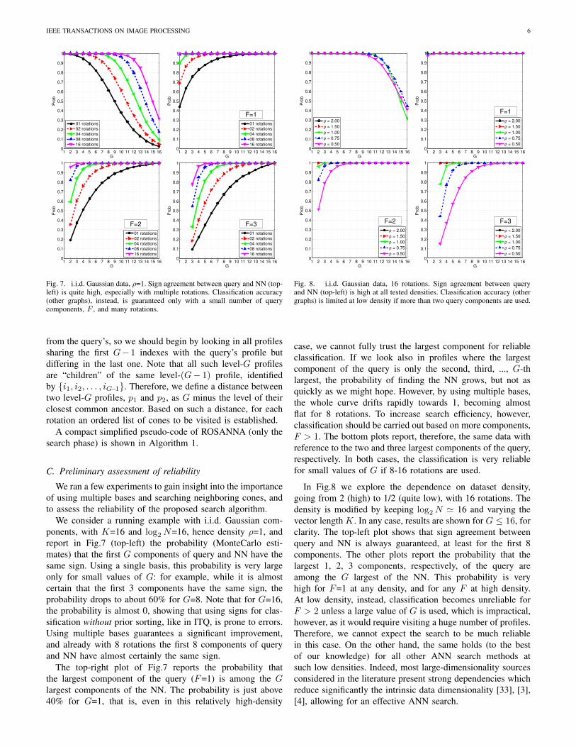
Fig. 7. i.i.d. Gaussian data, ρ=1. Sign agreement between query and NN (top-left) is quite high, especially with multiple rotations. Classification accuracy(other graphs), instead, is guaranteed only with a small number of querycomponents, F , and many rotations.

from the query’s, so we should begin by looking in all profilessharing the first G−1 indexes with the query’s profile butdiffering in the last one. Note that all such level-G profilesare “children” of the same level-(G− 1) profile, identifiedby i1, i2, . . . , iG−1. Therefore, we define a distance betweentwo level-G profiles, p1 and p2, as G minus the level of theirclosest common ancestor. Based on such a distance, for eachrotation an ordered list of cones to be visited is established.

A compact simplified pseudo-code of ROSANNA (only thesearch phase) is shown in Algorithm 1.

C. Preliminary assessment of reliability

We ran a few experiments to gain insight into the importanceof using multiple bases and searching neighboring cones, andto assess the reliability of the proposed search algorithm.

We consider a running example with i.i.d. Gaussian com-ponents, with K=16 and log2N=16, hence density ρ=1, andreport in Fig.7 (top-left) the probability (MonteCarlo esti-mates) that the first G components of query and NN have thesame sign. Using a single basis, this probability is very largeonly for small values of G: for example, while it is almostcertain that the first 3 components have the same sign, theprobability drops to about 60% for G=8. Note that for G=16,the probability is almost 0, showing that using signs for clas-sification without prior sorting, like in ITQ, is prone to errors.Using multiple bases guarantees a significant improvement,and already with 8 rotations the first 8 components of queryand NN have almost certainly the same sign.

The top-right plot of Fig.7 reports the probability thatthe largest component of the query (F=1) is among the Glargest components of the NN. The probability is just above40% for G=1, that is, even in this relatively high-density

1 2 3 4 5 6 7 8 9 10 11 12 13 14 15 160

0.1

0.2

0.3

0.4

0.5

0.6

0.7

0.8

0.9

1

G

Pro

b

ρ = 2.00

ρ = 1.50

ρ = 1.00

ρ = 0.75

ρ = 0.50

1 2 3 4 5 6 7 8 9 10 11 12 13 14 15 160

0.1

0.2

0.3

0.4

0.5

0.6

0.7

0.8

0.9

1

G

Pro

b

F=1

ρ = 2.00

ρ = 1.50

ρ = 1.00

ρ = 0.75

ρ = 0.50

1 2 3 4 5 6 7 8 9 10 11 12 13 14 15 160

0.1

0.2

0.3

0.4

0.5

0.6

0.7

0.8

0.9

1

G

Pro

b

F=2

ρ = 2.00

ρ = 1.50

ρ = 1.00

ρ = 0.75

ρ = 0.50

1 2 3 4 5 6 7 8 9 10 11 12 13 14 15 160

0.1

0.2

0.3

0.4

0.5

0.6

0.7

0.8

0.9

1

G

Pro

b

F=3

ρ = 2.00

ρ = 1.50

ρ = 1.00

ρ = 0.75

ρ = 0.50

Fig. 8. i.i.d. Gaussian data, 16 rotations. Sign agreement between queryand NN (top-left) is high at all tested densities. Classification accuracy (othergraphs) is limited at low density if more than two query components are used.

case, we cannot fully trust the largest component for reliableclassification. If we look also in profiles where the largestcomponent of the query is only the second, third, ..., G-thlargest, the probability of finding the NN grows, but not asquickly as we might hope. However, by using multiple bases,the whole curve drifts rapidly towards 1, becoming almostflat for 8 rotations. To increase search efficiency, however,classification should be carried out based on more components,F > 1. The bottom plots report, therefore, the same data withreference to the two and three largest components of the query,respectively. In both cases, the classification is very reliablefor small values of G if 8-16 rotations are used.

In Fig.8 we explore the dependence on dataset density,going from 2 (high) to 1/2 (quite low), with 16 rotations. Thedensity is modified by keeping log2N ' 16 and varying thevector length K. In any case, results are shown for G ≤ 16, forclarity. The top-left plot shows that sign agreement betweenquery and NN is always guaranteed, at least for the first 8components. The other plots report the probability that thelargest 1, 2, 3 components, respectively, of the query areamong the G largest of the NN. This probability is veryhigh for F=1 at any density, and for any F at high density.At low density, instead, classification becomes unreliable forF > 2 unless a large value of G is used, which is impractical,however, as it would require visiting a huge number of profiles.Therefore, we cannot expect the search to be much reliablein this case. On the other hand, the same holds (to the bestof our knowledge) for all other ANN search methods atsuch low densities. Indeed, most large-dimensionality sourcesconsidered in the literature present strong dependencies whichreduce significantly the intrinsic data dimensionality [33], [3],[4], allowing for an effective ANN search.

IEEE TRANSACTIONS ON IMAGE PROCESSING 7

0.990.90010

0

101

102

speed u

p

accuracy

E2LSH

IMIRKDT

HKM

FLANNIVFADC

ROSANNA

0.990.90010

0

101

102

speed u

p

accuracy

E2LSH

IMIRKDT

HKM

FLANNIVFADC

ROSANNA

0.990.90010

0

101

102

speed u

p

accuracy

E2LSH

IMIRKDT

HKM

FLANNIVFADC

ROSANNA

Fig. 9. Experimental results at ρ=1 with Gaussian (left), Uniform (center), and Laplace (right) i.i.d. data. In all cases ROSANNA, outperforms all references,sometimes by an order of magnitude, and results are only weakly affected by the data pdf.

N number of dataset vectorsK vector lengthG number of components used for queryNC number of cones, NC =

(KG

)2G

R number of rotations (hash tables)C number of cones visited for each rotation

TABLE IMAIN PARAMETERS OF THE ALGORITHM.

D. Assessment of complexity

We can now provide a theoretical assessment of compu-tational complexity, keeping in mind, however, that someprocessing steps include random components that may af-fect results significantly. To this end, Tab.I lists the mainparameters of the algorithm and the associated symbols, whileTab.II reports the complexity assessment as a function of thesequantities.

The dataset preparation phase is normally of minor interestsince it is carried out off-line once and for all. Considering thatN is much larger than K, the dominant term of this phaseis the rotation of the dataset points along the R bases. Weare considering the use of structured orthonormal matrices,like DCT or Walsh-Hadamard, in place of pseudo-randommatrices, which may reduce this cost. Hashing, instead, hasmore limited cost, related to vector sorting.

For on-line NN search the most critical item is typicallythe linear search of the candidate short-list where the distancefrom query to all candidates must be computed. However,the corresponding entry in Tab.II is only an approximation,based on the assumptions that dataset points are uniformlydistributed among the cones, and that the visited cones in-clude disjoint sets of points. The first assumption is prettyreasonable, the second much less. When multiple rotationsare used, it is very likely that some points are visited morethan once, in which case the distance is not computed anew.Therefore, our estimate is a bit pessimistic, but how muchso depends on many parameters. We can however single outbest and worst cases. In the best case, the shortlist includesonly one candidate, and search complexity is dominated by thecost of query rotation O(RK2). In the worst case, the shortlist

phase action complexitygenerate rotation matrices O(RK3)

dataset preparation rotate dataset points O(NRK2)

hash dataset points O(NRK log(K))

rotate query O(RK2)

NN search hash query O(RK log(K))

search short-list O(RCK(N/NC))

TABLE IICOMPLEXITY ASSESSMENT.

includes all dataset points, coming down to linear search, withcost NK.

In next Section, ROSANNA will be applied also to longvectors (e.g., 128 components) reduced to shorter unstructuredvectors through PCA and random rotation. Taking into accountalso the estimation of covariance matrix and the PCA, andthe use of partial distance elimination techniques, the aboveanalysis holds with minor adjustments also in such a case.

IV. EXPERIMENTAL ANALYSIS

We carried out a number of experiments to assess the per-formance of the proposed method. Results are given in termsof accuracy-efficiency plots, as in [15], [34] with accuracymeant as the probability that the selected point is the actual NN(also called precision and recall@1), and efficiency measuredin terms of speed-up w.r.t. linear search. The software iswritten in C++ using open libraries and some routines of theFLANN package4, and is published online5 to guarantee fullreproducibility of results. There are only a few parameters toset: the number of components used for classification, G, thenumber of rotations, R, used for multiple-basis search, and thenumber of visited cones per basis, C. In the preparation phase,for each rotation, all dataset points are projected on the newbasis and classified according to the index and sign of their Glargest components. Therefore we need R hash tables, with arelative memory overhead of R/K. A second-level hash table

4http://www.cs.ubc.ca/research/flann/5http://www.grip.unina.it

IEEE TRANSACTIONS ON IMAGE PROCESSING 8

0.990.90010

0

101

102

speed u

p

accuracy

E2LSH

IMIRKDT

HKM

FLANNIVFADC

ROSANNA

0.990.90010

0

101

102

speed u

p

accuracy

E2LSH

IMIRKDT

HKM

FLANNIVFADC

ROSANNA

0.990.90010

0

101

102

speed u

p

accuracy

E2LSH

IMIRKDT

HKM

FLANNIVFADC

ROSANNA

Fig. 10. Experimental results with Gaussian i.i.d. data at high (ρ=1.5, left), medium (ρ=1, center), and low (ρ=0.75, right) density. Performance dependsstrongly on density. ROSANNA works much better than the references at high density, and is on par with HKM at low density. In the latter case, a verylimited speed-up is obtained anyway.

is used to manage the tables when the number of cones growsvery large.

We compare results with a number of relevant state-of-the-art references: i) plain Euclidean LSH (E2LSH) [35] withthe implementation available online6 including the automaticsetting of most parameters; ii) randomized kd-trees (RKDT)and, iii) hierarchical k-means (HKM), both implemented in theFLANN package [15], together with iv) FLANN itself, whichis always inferior to the the best of RKDT and HKM butsets automatically all parameters; v) the IVFADC algorithm[1], based on product quantization, and implemented by usstarting from the Matlab code published by the authors7, andfinally vi) Inverted Multi-Index (IMI) [2] developed by theauthors8 except for the final linear search among candidates,which we carried out as in ROSANNA. All these techniquesare implemented in C++ language. We also implementedand run optimized PQ, both parametric and non-parametric[4], but did not include results, generally worse than thoseof the PQ-based IMI and IVFADC, in order not to clutterfurther the figures. Curves are obtained (except for FLANN)as the upper envelope, in the accuracy-time plane, of pointscorresponding to different parameter settings. For ROSANNA,we consider G ∈ 1, 2, . . . ,K/2, R ∈ 1, 2, 4, 8, 16, C ∈1, 2, 4, . . . , 128, and similar wide grids are explored forthe main parameters of all other techniques. To focus on themore interesting high-accuracy range, in all graphs we use alogarithmic scale for both accuracy and speed-up.

A. Unstructured data

Fig.9 (left) shows results for our running example, Gaussiani.i.d. data, k=16, ρ=1. ROSANNA guarantees uniformly thebest performance, being almost twice as fast than the secondbest, HKM, at all levels of accuracy, and much faster thanall the other references, gaining a full order of magnitudew.r.t. RKDT and E2LSH. The FLANN curve lies somewhatbelow HKM, since the parameters are selected in advance and

6http://www.mit.edu/∼andoni/LSH/7http://people.rennes.inria.fr/Herve.Jegou/projects/ann.html8http://arbabenko.github.io/MultiIndex/

may turn out not to be the best possible. However, we couldnot compute results for FLANN at high accuracy due to thelarge time needed to optimize the parameters. In Fig.9 wealso shows results obtained in the same conditions as beforebut using Uniform (left) and Laplace (right) random variablesin place of Gaussian. The general behavior is the same asbefore, with slight improvements observed in the Uniformcase, probably due to the smaller entropy.

With Fig.10 we go back to the Gaussian case, but changethe dataset density considering ρ =1.5 (left), ρ =1.0 (center)as before, for ease of comparison, and ρ =0.75 (right). Asexpected, ROSANNA works especially well at high density,while its performance becomes very close to the best reference,HKM, at lower density. In this latter case, however, a signif-icant speed-up can be obtained only at pretty low accuracy,whatever the technique used.

B. Structured data

Previous experiments confirm that ROSANNA works verywell with unstructured data. It can be argued, however, thatmost real-world datasets are highly structured, and oftenhave large dimensionality. Therefore, we now consider somepopular structured sources, SIFT descriptors [36], and MNISTimages of handwritten digits, often used to test the perfor-mance of ANN search algorithms. In particular we will usethe 100K-vector UBC SIFT dataset9, the 1M-vector IRISASIFT dataset10, and the 60K-vector MNIST database11, withthe train/test split coming with each one. SIFT vectors havelength 128, while MNIST images comprise 784 pixels. In bothcases, we search the datasets based on reduced-dimensionalityvectors. First, we compute the PCA and project the pointson the new basis, and then classify the data based only onthe first 16 components, which account for a large fractionof the energy (about 70% for the SIFT datasets and 60%for the MNIST database). In any case, the NN is searchedamong the selected candidates by computing distances over

9http://people.cs.ubc.ca/∼mariusm/uploads/FLANN/datasets/sift100K.h510http://corpus-texmex.irisa.fr/11http://yann.lecun.com/exdb/mnist/

IEEE TRANSACTIONS ON IMAGE PROCESSING 9

0.990.90010

1

102

103

speed u

p

accuracy

E2LSH

IMIRKDT

HKM

FLANNIVFADC

ROSANNA

0.990.90010

1

102

103

speed u

p

accuracy

E2LSH

IMIRKDT

HKM

FLANNIVFADC

ROSANNA

0.990.90010

1

102

103

speed u

p

accuracy

E2LSHIMI

RKDT

HKMFLANN

IVFADC

ROSANNAROSANNA+

Fig. 11. Experimental results with real-world data. Left: 100K UBC SIFT; center: 60K MNIST; right: 1M IRISA SIFT. ROSANNA outperforms almostuniformly all reference techniques in the first two cases. The same happens in the third case after k-means clustering (ROSANNA+).

0 10 20 30 400

0.05

0.1

0.15

0.2

0.25

0.3

0 10 20 30 400

0.2

0.4

0.6

0.8

1

Fig. 12. Normalized eigenvalues (left) and their cumulative sum (right) fortwo SIFT datasets. Energy distribution is highly skewed, with more than 70%of the energy in the first 16 components. The intrinsic data dimensionality ismuch smaller than 128.

all components, using partial distance elimination (PDE) [37]to speed-up the process.

The use of PCA is motivated by the need to reduce com-plexity and, a posteriori, by experimental evidence. However,it is also justified by the observation that the intrinsic dimen-sionality of real-world data is typically much smaller than theirnominal dimensionality. SIFT descriptors, for example, havea nominal dimensionality of 128, but the components are alsostrongly correlated. In Fig.12 we show, for both the UBC andthe IRISA datasets, the first 48 normalized eigenvalues λi (a),which account for the distribution of energy among the vectorcomponents after taking the PCA, and their cumulative sum(b). In both cases, and especially for IRISA, the distributionis very far from uniform, with most eigenvalues very close tozero, and 70% of the total energy in the first 16 components.Therefore, the intrinsic data dimensionality is much smallerthan 128. A rough estimate is

D∗ = 2H(p) (5)

where H(p) is the informational entropy, and pi =λi/∑i(λi). With this definition, the intrinsic dimensionality

drops to 38.69 for UBC and 27.94 for IRISA. Of course, thisestimate neglects non-linear dependencies, quite significantfor SIFT data (and MNIST as well), so the true intrinsicdimensionality is arguably even smaller.

Results are reported in Fig.11. In general, a much largerspeed-up is obtained w.r.t. to the case of unstructured data

(notice the decade shift on the y-axis) and no obvious lossof accuracy is observed due to the classification performedonly on 16 components. On both the UBC SIFT and MNISTdatasets, ROSANNA outperforms all reference techniques inthe medium-accuracy and especially high-accuracy range. Inthe 0.9–0.99 accuracy range, it is about twice as fast asthe best competitors. The situation changes with the IRISASIFT dataset, where all techniques, including ROSANNA(and except E2LSH), provide a comparable performance. Thereason lies in the much stronger structure of the IRISAdata, where the first PCA component accounts for almost33% of the total energy, as opposed to just above 10% forUBC data (the dataset size is, instead, immaterial, as thesame behavior is observed with 100K vectors). This is notsurprising, since ROSANNA is not designed to exploit datadependencies. In this case, the best performance is provided byIVFADC, which performs a preliminary k-means clustering,thus exploiting major data dependencies, before resorting toproduct quantization within a restricted number of clusters. Weresorted therefore to a similar solution to adapt ROSANNA tothe case of highly dependent data. Data are clustered off-lineby k-means. At search time, the query is compared with thecluster centroids, and only the nearest clusters are analyzedwith ROSANNA, collecting the candidates that are eventuallysearched for the NN. The overall search time is roughly halvedw.r.t. the basic version, providing much better results than allreferences, including IVFADC, especially at high accuracies.Preliminary k-means clustering is instead ineffective with theless structured UBC SIFT and MNIST data.

We conclude this analysis by showing, in Tab.III, inspiredto Tab.I of [15], some numerical performance figures ofROSANNA for the 100K UBC-SIFT dataset as a functionof its main parameters. In the first line we consider a pivotconfiguration with speed-up 100, while the following sixlines (labeled G−, G+, R−, R+, C−, C+) provide someinsight into the effect of increasing/decreasing only one of theparameters at a time w.r.t. the pivot. By increasing G, narrowercones are generated, leading to faster search (remember thatthe other parameters are fixed) but lower accuracy, while theopposite happens when G decreases. Operating on R and Cproduces similar effects, slower search and higher accuracy

IEEE TRANSACTIONS ON IMAGE PROCESSING 10

configuration parameters accuracy search memory build

G R C speed-up overhead time

pivot 4 8 4 0.905 100 0.36 0.36

G− 3 8 4 0.961 37 0.16 0.35

G+ 5 8 4 0.814 168 0.69 0.36

R− 4 4 4 0.788 180 0.18 0.26

R+ 4 16 4 0.966 54 0.71 0.57

C− 4 8 2 0.841 145 0.36 0.35

C+ 4 8 8 0.946 66 0.36 0.36

high speed 6 2 16 0.595 404 0.24 0.20

high accu. 3 16 8 0.999 14 0.30 0.56

low memory 3 1 128 0.901 18 0.03 0.17

TABLE IIIPERFORMANCE FIGURES FOR VARIOUS PARAMETER CONFIGURATIONS.

MEMORY OVERHEAD AND BUILD TIME ARE RELATIVE TO DATASETOCCUPATION AND LINEAR SEARCH TIME FOR THE TEST SET,

RESPECTIVELY.

when the parameter grows, and the opposite when it decreases.In all these cases, there is a nearly linear relationship betweenaccuracy and speed-up, when one grows the other decreases.Memory overhead, instead, exhibits a more varied behavior. Itremains constant when operating on C, since the data structuredoes not change. It is positively correlated with speed whenoperating on G, because faster search is obtained by definingmore cones. On the contrary, it is negatively correlated withspeed when operating on R, because faster search is obtainedby using less rotations. Therefore, one can keep memory lowboth when high-speed is required (reducing R) and when highaccuracy is required (reducing G). This is reflected in thenext two configurations, selected to guarantee high speed, andhigh accuracy, respectively, where memory overhead is alwaysrelatively low. The last configuration instead has almost nomemory overhead and still a good performance.

C. Fast copy-move forgery detection

With the diffusion of powerful image editing tools, imagemanipulation, often with malicious and dangerous aims, hasbecome easy and widespread. Copy-move is one of the mostcommon attacks, where a piece of the image is cut and pastesomewhere else in the same image to hide some undesiredobjects. Using material drawn from the same target image, infact, raises the likelihood to escape the scrutiny of a casualobserver.

The most effective copy-move detectors [38], [39], [7] arebased on dense feature matching. A feature is associated witheach block, and the most similar feature is searched for overthe whole image. Eventually, a dense field of offsets linkingcouple of pixels is obtained which, after some suitable post-processing, may reveal the presence of near-duplicate regions.By using scale/rotation invariant features, copy-moves canbe effectively detected even in the presence of geometricaldistortions.

Feature matching is the most computation-intensive phase ofcopy-move detection algorithms. In [7], this task is carried out

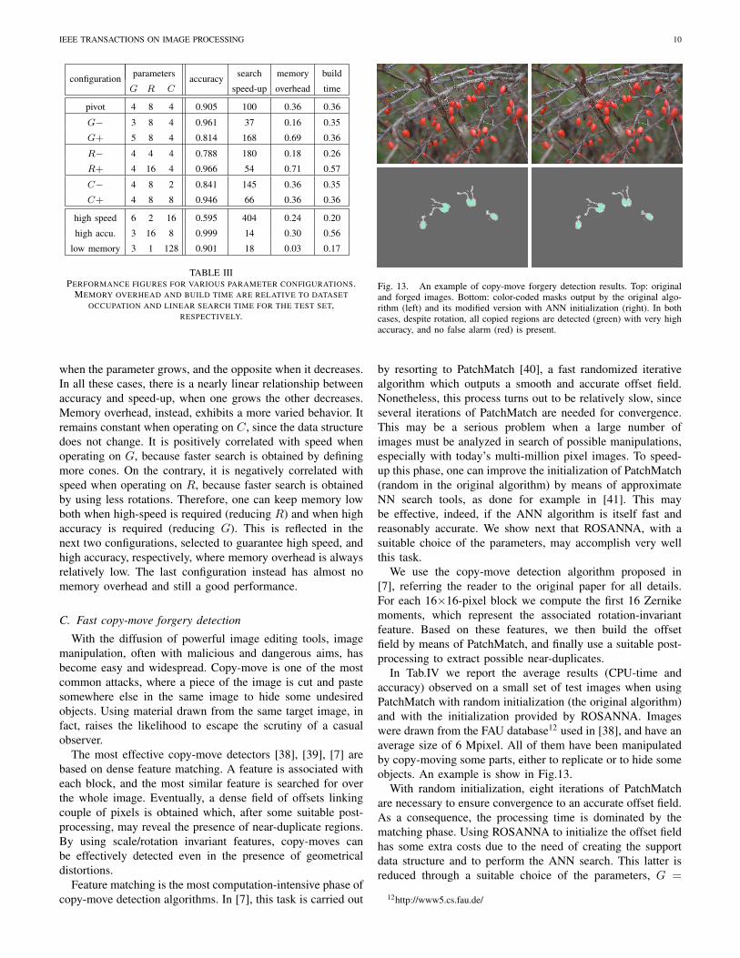
Fig. 13. An example of copy-move forgery detection results. Top: originaland forged images. Bottom: color-coded masks output by the original algo-rithm (left) and its modified version with ANN initialization (right). In bothcases, despite rotation, all copied regions are detected (green) with very highaccuracy, and no false alarm (red) is present.

by resorting to PatchMatch [40], a fast randomized iterativealgorithm which outputs a smooth and accurate offset field.Nonetheless, this process turns out to be relatively slow, sinceseveral iterations of PatchMatch are needed for convergence.This may be a serious problem when a large number ofimages must be analyzed in search of possible manipulations,especially with today’s multi-million pixel images. To speed-up this phase, one can improve the initialization of PatchMatch(random in the original algorithm) by means of approximateNN search tools, as done for example in [41]. This maybe effective, indeed, if the ANN algorithm is itself fast andreasonably accurate. We show next that ROSANNA, with asuitable choice of the parameters, may accomplish very wellthis task.

We use the copy-move detection algorithm proposed in[7], referring the reader to the original paper for all details.For each 16×16-pixel block we compute the first 16 Zernikemoments, which represent the associated rotation-invariantfeature. Based on these features, we then build the offsetfield by means of PatchMatch, and finally use a suitable post-processing to extract possible near-duplicates.

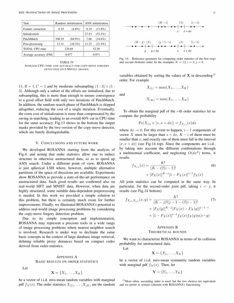
In Tab.IV we report the average results (CPU-time andaccuracy) observed on a small set of test images when usingPatchMatch with random initialization (the original algorithm)and with the initialization provided by ROSANNA. Imageswere drawn from the FAU database12 used in [38], and have anaverage size of 6 Mpixel. All of them have been manipulatedby copy-moving some parts, either to replicate or to hide someobjects. An example is show in Fig.13.

With random initialization, eight iterations of PatchMatchare necessary to ensure convergence to an accurate offset field.As a consequence, the processing time is dominated by thematching phase. Using ROSANNA to initialize the offset fieldhas some extra costs due to the need of creating the supportdata structure and to perform the ANN search. This latter isreduced through a suitable choice of the parameters, G =

12http://www5.cs.fau.de/

IEEE TRANSACTIONS ON IMAGE PROCESSING 11

Task Random initialization ANN initialization

Feature extraction 6.19 (4.8%) 6.19 (11.8%)

Initialization – 27.43 (52.2%)

PatchMatch 100.19 (84.9%) 7.66 (14.6%)

Post-processing 13.31 (10.3%) 11.22 (21.4%)

TOTAL CPU-time 129.69 52.50

Average accuracy (FM) 0.977 0.971

TABLE IVAVERAGE CPU-TIME AND ACCURACY FOR COPY-MOVE FORGERY

DETECTION ON 6 MPIXEL IMAGES.

11, R = 1, C = 1 and by moderate subsampling (1 : 3)× (1 :3). Although only a subset of the offsets are initialized, due tosubsampling, this is more than enough to ensure convergenceto a good offset field with only two iterations of PatchMatch.In addition, the random search phase of PatchMatch is skippedaltogether, reducing the cost of a single iteration. Eventually,the extra cost of initialization is more than compensated by thesaving in matching, leading to an overall 60% cut in CPU-timefor the same accuracy. Fig.13 shows in the bottom the outputmasks provided by the two version of the copy-move detector,which are barely distinguishable.

V. CONCLUSIONS AND FUTURE WORK

We developed ROSANNA starting from the analysis ofFig.4, and noting that order statistics allow one to inducestructure in otherwise unstructured data, so as to speed upANN search. Under a different point of view, ROSANNAis just spherical LSH where, however, multiple alternativepartitions of the space of directions are available. Experimentsshow ROSANNA to provide a state-of-the-art performance onunstructured data. Such good results are confirmed also onreal-world SIFT and MNIST data. However, when data arehighly structured, some suitable data-dependent preprocessingis needed. In this work we provided a simple solution tothis problem, but there is certainly much room for furtherimprovements. Finally, we illustrated ROSANNA’s potential toaddress real-world image processing problems by consideringthe copy-move forgery detection problem.

Due to its simple conception and implementation,ROSANNA may represent a precious tools in a wide rangeof image processing problems where nearest neighbor searchis involved. Research is under way to declinate the samebasic concepts in the context of large database image retrieval,defining reliable proxy distances based on compact codesderived from order-statistics.

APPENDIX ABASIC RESULTS ON ORDER STATISTICS

LetX = X1, . . . , XK

be a vector of i.i.d. zero-mean random variables with marginalpdf fX(x). The order statistics X(1), . . . , X(K) are the random

-(K−i)

x

(1)

x+dx

(i−1)r r r r r r r r r r r r

-(K−j)

y

(1)

y+dy

(j−1−i)

x

(1)

x+dx

(i−1)r r r r r r r r r r r rFig. 14. Reference geometry for computing order statistics of the first (top)and second (bottom) order. In the examples K = 12, i = 3, j = 9.

variables obtained by sorting the values of X in descending13

order. For example

X(1) = max(X1, . . . , XK)

andX(K) = min(X1, . . . , XK)

To obtain the marginal pdf of the i-th order statistics let uscompute the probability

Pr(X(i) ∈ [x, x+ dx]) = fX(i)(x)dx

where dx→ 0. For this event to happen, i− 1 components ofvector X must be larger than x+ dx, K − i of them must besmaller than x, and exactly one of them must fall in the interval[x, x + dx] (see Fig.14 top). Since the components are i.i.d.,by taking into account the different combinations througha multinomial coefficient, and neglecting O(dx2) terms, itresults

fX(i)(x) =

K!

(K − i)!(i− 1)!(6)

× [FX(x)]K−i[1− FX(x)]i−1fX(x)

All joint statistics can be computed in the same way. Inparticular, for the second-order joint pdf, taking i < j, itresults (see Fig.14 bottom)

fX(i)X(j)(x, y) =

K!

(K − j)!(j − 1− i)!(i− 1)!(7)

× [FX(y)]K−j [FX(x)− FX(y)]j−1−i

× [1− FX(x)]i−1fX(x)fX(y)u(x−y)

APPENDIX BTHEORETICAL BOUNDS

We want to characterize ROSANNA in terms of its collisionprobability for unstructured data.

LetX = X1, . . . , XK

be a vector of i.i.d. zero-mean symmetric random variableswith marginal pdf fX(x). Then, let

Y = Y1, . . . , YK

13More often, ascending order is used, but the two choices are equivalentand we prefer to remain coherent with ROSANNA’s functioning.

IEEE TRANSACTIONS ON IMAGE PROCESSING 12

-y1

6

y2

c1

Ω

c1\Ω

@@@@@

@@@ &%

'$rx

@@∆

hhrθ

Fig. 15. Geometry of the problem in 2d.

be a second vector which, given X = x, is uniformlydistributed on the hypersphere of radius r centered on x, thatis

fY(y|x) =1

SK(r)δ(‖y − x‖ − r)

where SK(r) is the measure of the K-d hypersphere of radiusr, and δ(·) is the Dirac delta function. We want to compute,for any radius r, the probability that X and Y belong to thesame cone

pcoll(r) = Pr[h(X) = h(Y)]

where the hash function h(·) associates a vector to a givencone based on the index and sign of its G largest components.Rather than the probability of collision, we will consider itscomplement

pcross(r) = 1− pcoll(r)

which is the probability that point Y lies across any of theboundaries of X’s cone.

A. The 2d case

Let us begin by considering the simplest non-trivial case ofK = 2 and G = 1. Fig.15 provides a pictorial description ofour problem in this setting. In the example, point x belongsto cone c1 where the first component is the largest, and it ispositive. In addition, we focus on the half-cone Ω where alsothe second component of x is positive

Ω = x ∈ R2 : x1 ≥ x2 ≥ 0

However, thanks to symmetry, all following arguments applyequally well to all other cones and half-cones with obviousmodifications. Therefore

pcross(r) = pcross(r |Ω) =

∫Ω

fX|Ω(x)pcross(r |x)dx (8)

Cone c1 has two boundaries, the lines with equations y2 = y1

and y2 = −y1. For each x in c1 let us label the boundaries inorder of increasing distance from x, so that

pcross,1(r |x)

is the probability of crossing boundary number 1, the nearestone. Let ∆ be the distance of x from this boundary. Since werestrict attention to Ω, this is

∆ = (x1 − x2)/√

2

0 1 2 3 40

0.1

0.2

0.3

0.4

0.5

0.6

0.7

0.8

0.9

1

point distance, r

P(c

ross|r

)

10−2

10−1

100

101

102

0

0.1

0.2

0.3

0.4

0.5

0.6

0.7

0.8

0.9

1

point distance, r

P(c

ross|r

)

Fig. 16. Theoretical bounds and MonteCarlo estimate for the crossingprobability in the case of i.i.d. standard Gaussian RV’s, with K=2, G=1.

while more in general it holds

∆ =max(|x1|, |x2|)−min(|x1|, |x2|)√

2

If ∆ < r, part of the circumference of radius r centered on xwill cross the nearest boundary. For our hypothesis of uniformdistribution of Y |x, the fraction of the circumference past theboundary represents the probability of crossing it

pcross,1(r |x) =

θ(r,∆)/π ∆ < r0 otherwise (9)

whereθ(r,∆) = arccos

(∆

r

)(10)

Of course, other points on the circumference may cross thesecond boundary, and some may cross both. Therefore (9)is only a lower bound to pcross(r|x). A good upper boundis obtained by the sum pcross,1(r|x) + pcross,2(r|x), whichmay be difficult to compute. Simpler but looser bounds are2 pcross,1(r|x) and 1 − 1/NC , with NC the total number ofcones. In summary

pcross,1(r|x)≤ pcross(r|x) (11)

≤ min

(2 pcross,1(r|x),

NC−1

NC

)and by averaging over X ∈ Ω we obtain lower and upperbounds for pcross(r).

In Fig.16 we plot these upper and lower bounds, togetherwith the actual crossing probability estimated through Monte-Carlo simulation, when the Xi’s are standard Gaussian RV’s.As expected, for small values of r the MonteCarlo estimateis very close to the theoretical lower bound (see also the log-scale plot on the right), while the gap grows when the distancebetween the two points, X and Y , becomes comparable withtheir own norm. When r → ∞, of course, Y belongs to anycone with the same probability, and the curve approaches thetheoretical upper bound of 3/4.

B. The general case

We now consider the general high-dimensional case, pro-ceeding in the very same way as for the 2d case, except forsome suitable modifications. The most important differencewith respect to the previous case is that we will resort to

IEEE TRANSACTIONS ON IMAGE PROCESSING 13

order statistics to reduce the final K-dimensional integral to anumerically tractable 2d integral.

In this case we have NC =(KG

)2G cones, statistically

indistinguishable from one another. Let us consider the conec1 where the first G components are also the largest, and theyare all positive. Furthermore, let us restrict attention to thesubregion of c1, call it again Ω, where also the smallest K−Gcomponents are all positive

Ω = x ∈ RK :min(x1, . . . , xG) ≥ max(xG+1, . . . , xK),

xi ≥ 0, i = 1, . . . ,K (12)

Again, because of symmetry, this restriction is immaterial, and(8) still holds. So, we will provide lower and upper boundsfor pcross(r|x), and then integrate over Ω.

Cone c1 is now delimited by 2G(K −G) hyperplanes, thehyper-planes with equations yi = yj and yi = −yj , for alli = 1, . . . , G and j = G + 1, . . . ,K, and the point Y atdistance r from x leaves the cone only if it crosses at leastone of such boundaries.

Let again ∆ be the distance of x from the closest boundary.If ∆ > r the probability of crossing that boundary (or anyother) is 0. Otherwise, it can be computed as the ratio betweenthe measure SK,∆(r) of the hyper-spherical cap intercepted bya hyperplane at distance ∆ from the center, and the measureSK(r) of the whole hyper-sphere. It is known that

SK(r) =2πK/2

Γ(K2 )rK−1

with Γ(·) the Gamma function, while the measure of the capcan be computed by integrating over θ the (K−1)-dimensionalhyper-spheres of radius r sin(θ)

SK,∆(r) =

∫ θ(r,∆)

0

SK−1(r sin(θ)) r dθ

where θ(r,∆) is still given by (10). As for ∆, note that theclosest boundary to x is the hyperplane of equation ym = yMwhere m is the index of the smallest component among the Glargest, and M is the index of the largest component amongthe K −G smallest. Consequently

∆ =xm − xM√

2

In summary it results

pcross,1(r |x) =

SK,∆(r)/SK(r) ∆ < r0 otherwise

Again, pcross,1(r|x) is a lower bound for pcross(r|x). An upperbound can be easily obtained as

pcross(r |x) ≤2G(K−G)∑

i=1

pcross,i(r|x)

≤ min

(2G(K −G)pcross,1(r|x),

NC − 1

NC

)As the last step of our development, we must compute the

integral (8) over X ∈ Ω which, for K 1, is computationallyintractable. However, we are not really interested in the K-

0 1 2 3 40

0.1

0.2

0.3

0.4

0.5

0.6

0.7

0.8

0.9

1

point distance, r

P(c

ross|r

)

10−2

10−1

100

101

102

0

0.1

0.2

0.3

0.4

0.5

0.6

0.7

0.8

0.9

1

point distance, r

P(c

ross|r

)

Fig. 17. Theoretical bounds and MonteCarlo estimate for the crossingprobability in the case of i.i.d. standard Gaussian RV’s, with K=16, G=4.

dimensional integral, since pcross,1(r |x) depends only on theG-th and (G+ 1)-st largest components of x through ∆, thatis,∫

Ω

fX|Ω(x)pcross,1(r |x)dx =∫ ∞0

∫ α

0

fX(G),X(G+1)|Ω(α, β)pcross,1(r |α, β)dβdα

where the X(i)’s are the order statistics obtained by sorting Xin descending order (remember that in Ω this coincides withsorting the vector for descending absolute values). Thereforewe only need the joint pdf of X(G) and X(G+1), which isgiven by (7).

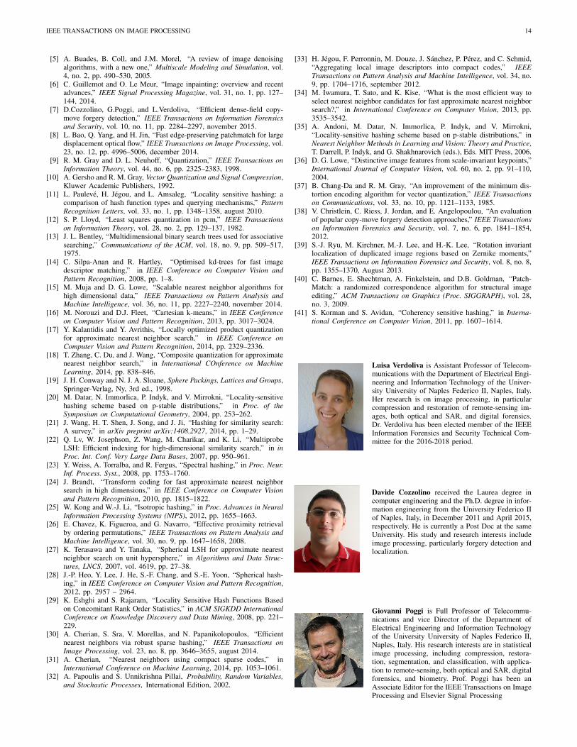
In Fig.17, we plot these upper and lower bounds, togetherwith the actual crossing probability estimated through Monte-Carlo simulation, when the Xi’s are standard Gaussian RV’s,for a single high-dimensional case, with K=16 and G=4.Again, for small values of r the MonteCarlo estimate is veryclose to the theoretical lower bound. The upper bound, instead,is too loose to be of practical guide.

These theoretical results confirm the correctness of theproposed algorithm. Close points tend to be hashed in thesame cell, and the collision probability approaches 1 as thedistance goes to 0. In addition, they can be used to guidethe choice of the algorithm parameters. One could computeupper and lower bounds for each value of K and G, andchoose the combination of parameters that better meets theproblem requirements. It is worth reminding that these resultshold rigorously only for the Gaussian i.i.d. case, and have beenobtained with reference to a simple version of the algorithm,with a single basis and no multi-probe. Nonetheless, theyrepresent a conceptual support to practical design.

REFERENCES

[1] H. Jegou, M. Douze, and C. Schmid, “Product quantization for nearestneighbor search,” IEEE Transactions on Pattern Analysis and MachineIntelligence, vol. 33, no. 1, pp. 117–128, january 2011.

[2] A. Babenko and V. Lempitsky, “The inverted multi-index,” in IEEEConference on Computer Vision and Pattern Recognition, 2012, pp.3069–3076.

[3] Y. Gong, S. Lazebnik, A. Gordo, and F. Perronin, “Iterative quantiza-tion: A procrustean approach to learning binary codes for large-scaleimage retrieval,” IEEE Transactions on Pattern Analysis and MachineIntelligence, vol. 35, no. 12, pp. 2916–2929, december 2013.

[4] T. Ge, K. He, Q. Ke, and J. Sun, “Optimized product quantization,”IEEE Transactions on Pattern Analysis and Machine Intelligence, vol.36, no. 4, pp. 744–755, april 2014.

IEEE TRANSACTIONS ON IMAGE PROCESSING 14

[5] A. Buades, B. Coll, and J.M. Morel, “A review of image denoisingalgorithms, with a new one,” Multiscale Modeling and Simulation, vol.4, no. 2, pp. 490–530, 2005.

[6] C. Guillemot and O. Le Meur, “Image inpainting: overview and recentadvances,” IEEE Signal Processing Magazine, vol. 31, no. 1, pp. 127–144, 2014.

[7] D.Cozzolino, G.Poggi, and L.Verdoliva, “Efficient dense-field copy-move forgery detection,” IEEE Transactions on Information Forensicsand Security, vol. 10, no. 11, pp. 2284–2297, november 2015.

[8] L. Bao, Q. Yang, and H. Jin, “Fast edge-preserving patchmatch for largedisplacement optical flow,” IEEE Transactions on Image Processing, vol.23, no. 12, pp. 4996–5006, december 2014.

[9] R. M. Gray and D. L. Neuhoff, “Quantization,” IEEE Transactions onInformation Theory, vol. 44, no. 6, pp. 2325–2383, 1998.

[10] A. Gersho and R. M. Gray, Vector Quantization and Signal Compression,Kluwer Academic Publishers, 1992.

[11] L. Pauleve, H. Jegou, and L. Amsaleg, “Locality sensitive hashing: acomparison of hash function types and querying mechanisms,” PatternRecognition Letters, vol. 33, no. 1, pp. 1348–1358, august 2010.

[12] S. P. Lloyd, “Least squares quantization in pcm,” IEEE Transactionson Information Theory, vol. 28, no. 2, pp. 129–137, 1982.

[13] J. L. Bentley, “Multidimensional binary search trees used for associativesearching,” Communications of the ACM, vol. 18, no. 9, pp. 509–517,1975.

[14] C. Silpa-Anan and R. Hartley, “Optimised kd-trees for fast imagedescriptor matching,” in IEEE Conference on Computer Vision andPattern Recognition, 2008, pp. 1–8.

[15] M. Muja and D. G. Lowe, “Scalable nearest neighbor algorithms forhigh dimensional data,” IEEE Transactions on Pattern Analysis andMachine Intelligence, vol. 36, no. 11, pp. 2227–2240, november 2014.

[16] M. Norouzi and D.J. Fleet, “Cartesian k-means,” in IEEE Conferenceon Computer Vision and Pattern Recognition, 2013, pp. 3017–3024.

[17] Y. Kalantidis and Y. Avrithis, “Locally optimized product quantizationfor approximate nearest neighbor search,” in IEEE Conference onComputer Vision and Pattern Recognition, 2014, pp. 2329–2336.

[18] T. Zhang, C. Du, and J. Wang, “Composite quantization for approximatenearest neighbor search,” in International COnference on MachineLearning, 2014, pp. 838–846.

[19] J. H. Conway and N. J. A. Sloane, Sphere Packings, Lattices and Groups,Springer-Verlag, Ny, 3rd ed., 1998.

[20] M. Datar, N. Immorlica, P. Indyk, and V. Mirrokni, “Locality-sensitivehashing scheme based on p-stable distributions,” in Proc. of theSymposium on Computational Geometry, 2004, pp. 253–262.

[21] J. Wang, H. T. Shen, J. Song, and J. Ji, “Hashing for similarity search:A survey,” in arXiv preprint arXiv:1408.2927, 2014, pp. 1–29.

[22] Q. Lv, W. Josephson, Z. Wang, M. Charikar, and K. Li, “MultiprobeLSH: Efficient indexing for high-dimensional similarity search,” in inProc. Int. Conf. Very Large Data Bases, 2007, pp. 950–961.

[23] Y. Weiss, A. Torralba, and R. Fergus, “Spectral hashing,” in Proc. Neur.Inf. Process. Syst., 2008, pp. 1753–1760.

[24] J. Brandt, “Transform coding for fast approximate nearest neighborsearch in high dimensions,” in IEEE Conference on Computer Visionand Pattern Recognition, 2010, pp. 1815–1822.

[25] W. Kong and W.-J. Li, “Isotropic hashing,” in Proc. Advances in NeuralInformation Processing Systems (NIPS), 2012, pp. 1655–1663.

[26] E. Chavez, K. Figueroa, and G. Navarro, “Effective proximity retrievalby ordering permutations,” IEEE Transactions on Pattern Analysis andMachine Intelligence, vol. 30, no. 9, pp. 1647–1658, 2008.

[27] K. Terasawa and Y. Tanaka, “Spherical LSH for approximate nearestneighbor search on unit hypersphere,” in Algorithms and Data Struc-tures, LNCS, 2007, vol. 4619, pp. 27–38.

[28] J.-P. Heo, Y. Lee, J. He, S.-F. Chang, and S.-E. Yoon, “Spherical hash-ing,” in IEEE Conference on Computer Vision and Pattern Recognition,2012, pp. 2957 – 2964.

[29] K. Eshghi and S. Rajaram, “Locality Sensitive Hash Functions Basedon Concomitant Rank Order Statistics,” in ACM SIGKDD InternationalConference on Knowledge Discovery and Data Mining, 2008, pp. 221–229.

[30] A. Cherian, S. Sra, V. Morellas, and N. Papanikolopoulos, “Efficientnearest neighbors via robust sparse hashing,” IEEE Transactions onImage Processing, vol. 23, no. 8, pp. 3646–3655, august 2014.

[31] A. Cherian, “Nearest neighbors using compact sparse codes,” inInternational Conference on Machine Learning, 2014, pp. 1053–1061.

[32] A. Papoulis and S. Unnikrishna Pillai, Probability, Random Variables,and Stochastic Processes, International Edition, 2002.

[33] H. Jegou, F. Perronnin, M. Douze, J. Sanchez, P. Perez, and C. Schmid,“Aggregating local image descriptors into compact codes,” IEEETransactions on Pattern Analysis and Machine Intelligence, vol. 34, no.9, pp. 1704–1716, september 2012.

[34] M. Iwamura, T. Sato, and K. Kise, “What is the most efficient way toselect nearest neighbor candidates for fast approximate nearest neighborsearch?,” in International Conference on Computer Vision, 2013, pp.3535–3542.

[35] A. Andoni, M. Datar, N. Immorlica, P. Indyk, and V. Mirrokni,“Locality-sensitive hashing scheme based on p-stable distributions,” inNearest Neighbor Methods in Learning and Vision: Theory and Practice,T. Darrell, P. Indyk, and G. Shakhnarovich (eds.), Eds. MIT Press, 2006.

[36] D. G. Lowe, “Distinctive image features from scale-invariant keypoints,”International Journal of Computer Vision, vol. 60, no. 2, pp. 91–110,2004.

[37] B. Chang-Da and R. M. Gray, “An improvement of the minimum dis-tortion encoding algorithm for vector quantization,” IEEE Transactionson Communications, vol. 33, no. 10, pp. 1121–1133, 1985.

[38] V. Christlein, C. Riess, J. Jordan, and E. Angelopoulou, “An evaluationof popular copy-move forgery detection approaches,” IEEE Transactionson Information Forensics and Security, vol. 7, no. 6, pp. 1841–1854,2012.

[39] S.-J. Ryu, M. Kirchner, M.-J. Lee, and H.-K. Lee, “Rotation invariantlocalization of duplicated image regions based on Zernike moments,”IEEE Transactions on Information Forensics and Security, vol. 8, no. 8,pp. 1355–1370, August 2013.

[40] C. Barnes, E. Shechtman, A. Finkelstein, and D.B. Goldman, “Patch-Match: a randomized correspondence algorithm for structural imageediting,” ACM Transactions on Graphics (Proc. SIGGRAPH), vol. 28,no. 3, 2009.

[41] S. Korman and S. Avidan, “Coherency sensitive hashing,” in Interna-tional Conference on Computer Vision, 2011, pp. 1607–1614.

Luisa Verdoliva is Assistant Professor of Telecom-munications with the Department of Electrical Engi-neering and Information Technology of the Univer-sity University of Naples Federico II, Naples, Italy.Her research is on image processing, in particularcompression and restoration of remote-sensing im-ages, both optical and SAR, and digital forensics.Dr. Verdoliva has been elected member of the IEEEInformation Forensics and Security Technical Com-mittee for the 2016-2018 period.

Davide Cozzolino received the Laurea degree incomputer engineering and the Ph.D. degree in infor-mation engineering from the University Federico IIof Naples, Italy, in December 2011 and April 2015,respectively. He is currently a Post Doc at the sameUniversity. His study and research interests includeimage processing, particularly forgery detection andlocalization.

Giovanni Poggi is Full Professor of Telecommu-nications and vice Director of the Department ofElectrical Engineering and Information Technologyof the University University of Naples Federico II,Naples, Italy. His research interests are in statisticalimage processing, including compression, restora-tion, segmentation, and classification, with applica-tion to remote-sensing, both optical and SAR, digitalforensics, and biometry. Prof. Poggi has been anAssociate Editor for the IEEE Transactions on ImageProcessing and Elsevier Signal Processing