wake-airfoil interaction as broadband noise source: …acoustique.ec-lyon.fr/publi/boudet_ija05.pdfm...

Wake-airfoil interaction as broadbandnoise source: a large-eddy simulation study

Jérôme Boudet†, Nathalie Grosjean, Marc C. JacobLaboratoire de Mécanique des Fluides et d’Acoustique (LMFA)

Ecole Centrale de Lyon/Université Claude Bernard Lyon 1/UMR CNRS 5509

36, avenue Guy de Collongue – 69134 Ecully Cedex – France

e-mail: [email protected]

ABSTRACTA large-eddy simulation is carried out on a rod-airfoil configuration and compared to anaccompanying experiment as well as to a RANS computation. A NACA0012 airfoil (chord c = 0.1 m) is located one chord downstream of a circular rod (diameter d = c/10, Red = 48 000).The computed interaction of the resulting sub-critical vortex street with the airfoil is assessedusing averaged quantities, aerodynamic spectra and proper orthogonal decomposition (POD) ofthe instantaneous flow fields. Snapshots of the flow field are compared to particle image velocimetry(PIV) data. The acoustic far field is predicted using the Ffowcs Williams & Hawkings acousticanalogy, and compared to the experimental far field spectra. The large-eddy simulation is shownto accurately represent the deterministic pattern of the vortex shedding that is described by PODmodes 1 & 2 and the resulting tonal noise also compares favourably to measurements. Furthermorehigher order POD modes that are found in the PIV data are well predicted by the computation.The broadband content of the aerodynamic and the acoustic fields is consequently well predictedover a large range of frequencies ([0 kHz; 10 kHz]).

NOMENCLATUREc airfoil chordC speed of sound in the medium at restCs Smagorinsky constantd rod diameteret total energyf frequencyf0 shedding frequencyk turbulent kinetic energyLexp spanwise extent in the experiment (30d)Lsim spanwise extent in the simulation (3d)

aeroacoustics volume 4 · number 1+2 · 2005 – pages 93 – 115 93

†now Research Fellow at the University of Surrey (UK) – TFS UTC.

IJA 4(1)P-06-Boudet 13/4/05 2:33 pm Page 93

M Mach numberp pressureq generic field quantityRed Reynolds number based on the rod diameterSij strain rate tensorSt Strouhal number of the vortex shedding

(St = f0.d/U∞, where f0 is the frequency of the vortex shedding)U mean flow velocity<u> local mean streamwise velocityu′ rms value of velocity fluctuations in local mean flow directionui velocity component in the ith direction (i = 1:x, i = 2:y, i = 3:z)Wij weighting factorx, y, z cartesian coordinates (cf. Figure 1) (origin at airfoil leading edge)r, θ, z cylindrical coordinates (x = r cosθ − c/2, y = r sinθ) for observer

point (origin at airfoil centre)δij Kronecker symbol∆c filter size∆x+, ∆y+, ∆z+ near wall mesh spacing in wall units (tangent to wall, normal

to wall and spanwise respectively)Γ 2 correlation functionλ bulk viscosityµ dynamic viscosity (µ = ρν)µsgs subgrid-scale viscosity (µsgs = ρνsgs)ρ densityσij deviatoric part of strain rate tensorω turbulent dissipation (model of Wilcox [28])

SUBSCRIPTS∞ upstream flow quantities

SUPERSCRIPTS— filter operator~ Favre operator

ABBREVIATIONSCFD computational fluid dynamicsDES detached-eddy simulationLES large-eddy simulationPIV particle image velocimetryPOD proper orthogonal decompositionPSD power spectral densityOGV outlet guide vanesRANS Reynolds averaged Navier-Stokesrms root mean square

94 Wake-airfoil interaction as broadband noise source


aeroacoustics volume 4 · number 1+2 · 2005 95

1. INTRODUCTIONMany practical applications involve flows governed by both deterministic and randommechanisms. On an aircraft, examples are numerous: periodic interaction of turbomachineblades with the turbulent wakes of the upstream blade row, interaction of slat cavitytones with airfoil boundary layer and wake, etc. Since these mechanisms lead to highnoise levels, they have been a major research topic for the last decades.

In aeronautics, the first studies were concerned with the deterministic part of suchflows. In particular, the aeolian tones of flows around cylinders have been a populararea of interest since Strouhal’s pioneering work [1]. For a single airfoil, the mostcommon noise source is of broadband nature as soon as the oncoming flow advects nonnegligible turbulence. Unsteady airfoil aerodynamics have therefore been very earlyoriented towards turbulence/airfoil interactions (e.g. references [2, 3, 4, 5, 6]). Theessence of these approaches is to decompose incoming turbulent flow perturbations intoharmonic gusts impinging the leading edge and to predict the resulting lift fluctuationsfrom a linear theory (Sears [5]). In the seventies, Widnall [7] and Amiet [8, 9] predictedthe broadband noise spectrum for single airfoils in turbulent flows by combining thesetheories with acoustic analogies. These theories were then extended to non-linearinteractions (Goldstein & Atassi [10]). Now efforts are spent to accompany and extendthese theoretical approaches by numerical ones for more complex geometries (airfoilswith slats and flaps) (e.g. [11]).

In parallel to Amiet’s work, similar approaches were developed for the prediction ofboth tonal and broadband noise generated by rotating blades for turbomachineryapplications. In 1974, Hanson [12] studied the noise radiated by a fan submitted toatmospheric turbulence, comparing his experiments with a spectral formulation based onmeasured turbulent statistics. Homicz and George [13] extended Amiet’s work to rotatingblades assuming the shape of the turbulent spectrum at the inlet and a lift response of theairfoil governed by an aerodynamic transfer function (depending on the turbulent wave-length). More recently, Majumdar and Peake [14] also focused on ingested atmosphericturbulence, following the work of Hanson, and formulated the influence of streamlinecontraction on turbulence using Rapid Distortion Theory. More recently, Glegg [15]included cascade effects into a rotor-stator interaction broadband noise model.

This kind of prediction is very useful to model both the tones and the statistics of thebroadband noise radiated by turbo-engines. However, as progress is made in aircraft noisereduction, the broadband contribution of engines (fan/OGV) and of high-lift devices to theoverall sound level tend to increase. Since all the state-of-the-art methods have alreadybeen applied, every new noise abatement requires more advanced and precise designtools. Because of the limits of the analytical approaches, that require simplifyingassumptions about the turbulent flow and the blade geometry, numerical approaches in thetime domain offer a promising alternative. As pointed out by the present authors inprevious studies [16, 17], only the deterministic part of a flow is predicted by solving theReynolds Averaged Navier-Stokes (RANS) equations that are as commonly used foraerodynamic design. The prediction of the broadband noise can be achieved by adding astochastic model for the turbulent fluctuations, such as proposed by Bailly et al. [18].However, such models are often limited to particular turbulent conditions.


Therefore, new CFD methods that were so far out of reach for aeroacoustic predictionsin complex flows, have to be considered in the light of currently available computerresources as a road map for future applications in an industrial environment. This is thecase of large-eddy simulation (LES), which predicts the larger turbulent structures of the flow down to the size of the spatial filter, assuming that their sound radiationdominates the lower end of the acoustic spectrum. The validity of this assumption hasbeen shown by Seror et al. [19], who compared a fully resolved DNS to a LES in thecase of isotropic homogeneous turbulence and showed that the subgrid scale eddies donot contribute to frequencies that are a few times smaller than the cut-off frequency.Consequently, in the present configuration an LES approach can be expected to allow theprediction of the acoustic spectrum up to a frequency of the order of the cut-offfrequency, which corresponds to the smallest resolved turbulent structures. For example,Terracol et al. [11] applied this idea to the prediction of trailing edge noise. A large-eddysimulation was used to predict the aerodynamic sources, but was not suited for acousticpropagation due to the different numerical requirements of the aerodynamic and acousticcomputations. In order to predict the far field, Terracol et al. computed the sources forthe Ffowcs Williams and Hawkings acoustic analogy [20], or used the Kirchhof integralequation [11] in the acoustic near field. This approach is particularly convenient forsimple propagation conditions, but for more complex configurations, including complexgeometries (e.g. turbo-engine nacelle) or inhomogeneous propagation media, alternativeComputational Aero-Acoustics methods have to be applied. The complex geometries canbe taken into account using an adapted Green function in the Ffowcs Williams andHawkings acoustic analogy (such Green functions generally need to be estimatednumerically) or using the well-known Boundary Elements Method. Also, semi-analyticalsolutions for propagation in tubes with varying cross-sectional area are available forducted flows and can be coupled with the far field approaches. Finally, the linearisedEuler equations allow to take into account both the complex geometries and the flowinhomogeneities, but the computational cost limits its application to the near field.Schönwald et al. [21] presented a review of such methods for turbo-engines.

In this context, the present study is a step towards complex multi-body configurations.The flow past an airfoil in the wake of a rod is a challenge for large-eddy simulation(LES) and a relevant configuration with regard to aeronautic applications, includingboth tonal and broadband noise sources.

In Section 2, the configuration, the experiment and the computational tools aredescribed. The main results are shown and discussed in Section 3, highlighting theinnovative analysis of the aerodynamic field in relation with the resulting acoustics.Finally, conclusions are drawn in Section 4.

2. METHODS AND APPROACHESBenchmark experimentThe CFD results are compared to those of a rod-airfoil experiment reported by Jacob et al. [22]. The experiment is carried out in the large anechoic room of the Ecole Centralede Lyon (10 m × 8 m × 8 m). A NACA 0012 airfoil (chord: c = 0.1m; thickness: 0.012 m)



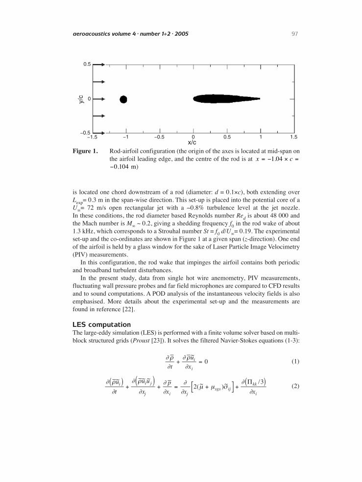
is located one chord downstream of a rod (diameter: d = 0.1×c), both extending overLexp= 0.3 m in the span-wise direction. This set-up is placed into the potential core of aU∞= 72 m/s open rectangular jet with a ∼0.8% turbulence level at the jet nozzle. In these conditions, the rod diameter based Reynolds number Red is about 48 000 andthe Mach number is M∞ ~ 0.2, giving a shedding frequency f0 in the rod wake of about1.3 kHz, which corresponds to a Strouhal number St = f0 d/U∞= 0.19. The experimentalset-up and the co-ordinates are shown in Figure 1 at a given span (z-direction). One endof the airfoil is held by a glass window for the sake of Laser Particle Image Velocimetry(PIV) measurements.

In this configuration, the rod wake that impinges the airfoil contains both periodicand broadband turbulent disturbances.

In the present study, data from single hot wire anemometry, PIV measurements,fluctuating wall pressure probes and far field microphones are compared to CFD resultsand to sound computations. A POD analysis of the instantaneous velocity fields is alsoemphasised. More details about the experimental set-up and the measurements arefound in reference [22].

LES computationThe large-eddy simulation (LES) is performed with a finite volume solver based on multi-block structured grids (Proust [23]). It solves the filtered Navier-Stokes equations (1-3):

(1)

(2)∂ ρ

∂

∂ ρ

∂∂∂

∂∂

µ µ σ∂

∂( )

/u

t

u u

x

p

x x xi i j

j i jsgs ij

kk

i

( )+

( )+ = +[ ] +

( )2

3Π~ ~ ~~ ~

∂ ρ∂

∂ ρ∂t

u

xi

i

+ =~

0


1.510.5−0.5−1.5−0.5

0

0.5

y/c

x/c−1 0

Figure 1. Rod-airfoil configuration (the origin of the axes is located at mid-span onthe airfoil leading edge, and the centre of the rod is at

)−0 104. mx c= − × =1 04.


(3)

where

and

Πkk is neglected according to Erlebacher [24], and νsgs is modelled by the auto-adaptivemodel of Casalino et al. [16, 22, 25]:

(4)

(5)

where Cs = 0.18, and ∆c is the local length scale of the filter (the cubic root of the cellvolume). corresponds to the summation over the 27 nearest points that surround each

mesh point, the grid being a 3D structured mesh with additional planes for the boundaryconditions. This model is based on the Smagorinsky model [26], but includes the factorWij to damp the strong gradients in the regions of high mean shear: for example near the wall, where the Smagorinsky model is too dissipative, the weight factors tend tozero following the van Driest law [27]. More information about the construction of thismodel and its validation (channel flow, isolated rod) can be found in the references [16, 22, 25].

The fluxes are interpolated by centred spatial schemes. A 4th order scheme is usedfor the convective fluxes, with a 4th order artificial dissipation defined by:

for the interface between points (i − 1) and i, where: |u| is the velocity in the considereddirection of the flux, C the speed of sound and q the considered field quantity on the fourpoint stencil (i − 2 to i + 1). This numerical viscosity creates a peripheral damping zone,

επ

= + × −( )( ) + × −( )( )( )0 10 11

50 0 2 50 0 1..

arctan | | . arctan | | .x y

F u C q q q qiAD

i i i i− − − += × +( ) × − + − +( )1 2 2 1 1386 13 13 6/ | |

ε

∑Nw

W

S

S

ij

ij

N

lmN

l m

w

w

=

∑

∑∑

91

1

3

3,

~

~

ν sgs s c ij ijC W S= 2 2 22∆ ƒ

Πij i j i ju u u u= − +ρ ρ~ ~

σ δij ij ij kkS S= −1

3S

u

x

u

xiji

j

j

i

= +

1

2

∂∂

∂

∂

∂ ρ

∂∂

∂ρ

∂∂

µ σ∂

∂µ σ

∂∂

λµ ∂

∂(

(e

t xe p u

xu u

x

xC

T

x

t

it i

ji ij i

jsgs ij

iv

sgs

t i

( )+ +( )[ ] = ( ) + ( )

+ +

Pr

2 2~ ~~ ~ ~ ~

~ ~



but vanishes for and in order to preserve the turbulent fluctuations. A 2nd

order scheme is used for the diffusive fluxes [23]. Time marching is explicit with a 5-stage Runge-Kutta algorithm [23].

The central part of the grid is shown on Figure 2: it extends over 100d and 50d in the stream-wise (x) and cross-stream (y) directions respectively, and over Lsim = 3d in thespan-wise direction (z). The rod and the airfoil surfaces are meshed with 205 and 353circumferential points respectively, at each span-wise location, and with 31 points alongthe span. The total number of points is about 2.4 million, divided into 32 grid blocks.On the airfoil, the grid density is characterised by: ∆x+ < 300 (< 85 for x/c < 0.13, i.e.in the leading edge region), ∆y+ < 1.25 and ∆z+ < 350, in the stream-wise, normal-to-wall and span-wise directions respectively. The resolution in the span-wise direction isquite low compared to wall flow scales, but since the turbulence is governed by thevortex shedding, which induces a strong correlation along z (the two-point pressurecorrelation length is about 3d on the side of the rod [16]), this spacing (31 points percorrelation length) is physically reasonable.

Boundary conditions are non-slip at the walls and non-reflecting on the outerboundaries (combined with a damping layer characterised by increased numerical viscosityand grid stretching), whereas a slip condition is applied to the planes limiting the span.This latter condition has been chosen to reduce the constraints on the flow field. Unlikeperiodicity conditions that fully correlate all the aerodynamic field quantities of thelimiting planes, the slip condition only imposes one component of velocity (z-component)to vanish and only affects the vicinity of the boundary. This condition is also physicallyrelevant: the mean value of the spanwise velocity is zero in the modelled flow. In a previouscomputation [16, 25], the two-point span-wise pressure correlation on the isolated rodwas proven to match the experimental one, which is of major importance for the acousticcomputations and cannot be achieved with a periodicity condition. Consequently, theslip condition allows a better comparison with the experiment that was carried out witha long span (Lexp= 30d).

| |y c≤| |x c≤ 2


Figure 2. Detail of the LES grid


The inflow is uniform in the inlet section, and the surrounding jet flow of theexperiment is not modelled. This is justified by the fact that the experimental rod-airfoilconfiguration was located in the potential core of the jet and that a few diameters awayin the cross-stream direction, the flow became uniform over several rod diametersbefore the jet shear layers were reached.

The LES computation is launched from a converged RANS computation (cf. nextsub-section), run over 6 cycles for further convergence and then recorded for 18 cycles.

As an example, the z-component of the instantaneous vorticity obtained from theLES computation is mapped in Figure 3. The main vortices shed from the rod (vonKármán vortices) impinge onto the airfoil and partly split at the leading edge. The airfoilwake can also be distinguished. Moreover, many smaller structures can be noticed inthe rod wake, due to the transition to turbulence in the shear layers of the rod. Thismultiple scale flow dominated by the large von Kármán vortices is a characteristicfeature of the rod-airfoil configuration in the sub-critical shedding regime.

Unsteady RANS computationAn unsteady RANS computation has been previously carried out [17], using the samecode and the k-ω turbulence model of Wilcox [28] (with an inflow turbulence levelu’/U∞ ~ 0.8%). The grid was only two-dimensional, because a three-dimensionalconfiguration similar to the LES one gave no difference with the 2D grid: the flow wasa span-wise repetition of the 2D flow. This is due to the averaged formulation of theRANS approach that does not predict turbulence as a fluctuating field and dampens outsmall perturbations. The RANS computation was considered converged when the pressureoscillations became periodic within ± 3%. This computation is compared to the LES.

Aeroacoustic computationsThe rotor noise code Advantia (Casalino [29]) is used for the acoustic prediction. Thiscode is based on the Ffowcs Willams & Hawkings analogy [20]. In the present


y

x

(rot v)z

10000.000

−10000.000

Figure 3. z-component of instantaneous vorticity from the LES computation


investigation it exploits the retarded time penetrable FW-H formulation proposed byBrentner & Farassat [30]. Only surface integrals are computed, since at the current Machnumber, the volume sources give a vanishing contribution to the acoustic radiation. Theconsistency of this approximation has been checked by Casalino et al. [31] for a RANScomputation of the rod-airfoil flow by comparing acoustic results obtained from differentintegration surfaces.

In the present paper, results are shown for a penetrable surface that surrounds theairfoil at a distance of one rod diameter (d ), and is defined on the CFD mesh points.Preliminary studies such as references [16, 25] as well as experimental results [22] haveshown that the rod contribution to the overall sound level is negligible with respect tothat of the airfoil. This surface contains the largest eddies of the flow around the airfoil.At the shedding frequency f0 = 1.3 kHz, the average surface resolution is of 356 pointsper wavelength in the circumferential direction, and 262 points per wave-length in thespan-wise direction. At 10 kHz, these values drop to 48 and 34 respectively.

3. RESULTS AND DISCUSSIONIn this section, typical results are discussed, first the velocity statistics, then the unsteadyfields (spectra) and instantaneous values, and finally the far field.

Velocity statisticsVelocity statistics are compared to single hotwire data: the mean velocity modulus<u>/U∞ and the corresponding rms velocity fluctuations in the local mean flowdirection u′ are plotted in Figure 4 and Figure 5 for two cross sections.

Figure 4 shows the profiles in the far rod wake at x/c = −0.255, that is about 7.5 roddiameters downstream of the rod. The LES provides a much more accurate descriptionof the mean velocity than the RANS computation. The narrower and smaller velocitydeficit in the RANS computation is due to the fact that separation on the rod is delayedas discussed in [16, 25]. Moreover on the LES predicted rms profile, the two mixinglayers have merged similarly to the experiment, whereas they are still distinct with highermaximal values in the RANS computation. In fact the RANS profile is quite close tothat predicted by potential flow. This seems to indicate that the turbulent diffusion isunderestimated in the RANS computation. Both computations predict slightly higherlevels than the measured ones. In the case of LES, this may be inferred to a lack of timeseries resulting in poorly converged statistics.

Figure 5 is dedicated to the section x/c = 0.25 near the airfoil thickest cross-section.Again, LES is much more accurate than RANS. In particular, the mean flow near thewall fits better to the hotwire data. The near wall region extends up to about y/c = 0.45in the LES whereas it is confined to y/c ≤ 0.3 in the RANS profile, with a pronouncedmaximum near y/c = 0.18. The shape of these profiles can be explained by the fact thatin this region the flow is the result of two tendencies: on one hand the influence of theairfoil onto the steady flow is to accelerate it; on the other hand the fluctuating flow isdominated by vorticity shed from the corresponding side (y = +d/2) of the rod that tendsto accelerate the flow away from the airfoil (the effect is strongest at the limit of thevortex core) and to slow it down near the wall. Again, the underestimated diffusion in




0.8

1

0.6

0.4

0.2

0−0.4 −0.2 0.2 0.4

experiment (hot-wire)RANS computationLES computation


y/c

<u>

/U∞

0

15

20

10

5

0−0.4 −0.2 0.2 0.4

y/c

u′ (

m/s

)

0

Figure 4. Mean velocity (top) and rms value of fluctuating velocity (bottom) at x/c = −0.255 (mid span z = 0). [Note: for the RANS computation,

u’ = where is the resolved velocity,is the mean flow direction, k the turbulent kinetic energy

and < > the time average]

r rn u u= < > < >/

ruu n u k( . ) /< − < > > + × < >

r r 2 2 3

IJA 4(1)P-06-Boudet 13/4/05 2:33 pm 2


0.8

1

0.6

0.40 0.2 0.4 0.6 0.8 1



y/c

<u>

/U∞

15

20

10

5

00 0.2 0.4 0.6 0.8 1

y/c

u′ (

m/s

)

Figure 5. Mean velocity (top) and rms value of fluctuating velocity (bottom) at x/c = 0.25 (mid span z=0). [Note: for the RANS computation,

u’ = where is the resolved velocity,

is the mean flow direction, k the turbulent kinetic energyand < > the time average]

r rn u u=< > < >/

ruu n u k( . ) /< − < > > + × < >

r r 2 2 3


the RANS results in a more concentrated vorticity and therefore the effect is strongerfor this computation. In the RANS solution, the well-organised vorticity patterns alsoresult in locally high fluctuation levels that do not reach so far out into the flow as theydo in the LES or in the experiment. Other evidences of this analysis will appear in thespectral analysis and in the instantaneous snapshots.

Spectral analysis of the aerodynamic fieldsAnother insight into this flow can be gained from the analysis of typical spectra, whichare expected to distinguish the broadband from the deterministic part of the fluctuations.Thus the spectrum obtained from a wall pressure probe located at x/c = 0.2 on thesurface of the airfoil, is plotted in Figure 6 and compared to the corresponding LES andRANS results.

All lines are dominated by the Strouhal peak of the rod shedding frequency. In theexperiment this frequency is f0 = 1 370 Hz, that is St = f0.d/U∞ = 0.19. This value of Stagrees with the values found in literature about vortex shedding from a circular cylindernear Red ∼ 4.8 × 104 [32]. On the experimental curve, the first harmonic can also bedistinguished although it hardly peaks out of the background noise. The second mainfeature of this spectrum is the twofold influence of sub-critical rod wake turbulence: itbroadens the main peak around the shedding frequency as a result of the interactionbetween the large von Kármán vortices and the multiple turbulent scales, and also


experiment (unsteady wall pressure probe)

RANS computationLES computation130

120

110

100

90

80

70

60

50

40

301000 10000

f (Hz)

PS

D (

dB)

Figure 6. Pressure spectrum at x/c = 0.2 on the airfoil


generates a broadband spectrum that is directly related to the flow turbulence and thatdecays slowly in the higher frequency range.

The level and the width of the peak, as well as the background turbulent spectrumare well predicted by LES. This remarkable result shows that the LES gives an accurateflow picture of both the deterministic and the random part of the flow, even near thecurved airfoil. Only the first harmonic does not clearly peak out of the broadbandspectrum as it does in the experiment.

Technically, the experimental spectrum results from the average of the spectracalculated on 200 samples and has a spectral resolution of 4 Hz. This is unaffordablefor the LES due to the prohibitive computational time that would be required in thisexplicit time approach. The present LES spectrum was obtained by averaging 31 singlepoint spectra over the span-wise direction and has a resolution of 72 Hz.

Finally, the quality of this LES spectrum is also highlighted by the comparison withthe RANS results.

The RANS spectrum in Figure 6 confirms the purely periodic deterministic nature ofthis flow. There is no broadband component due to turbulence since turbulence is onlymodelled by the averaged quantities k and ω. Furthermore, the shedding frequency isoverestimated by 25%, because of the inaccurate representation of the sub-criticalseparation on the rod [16, 25] (delayed separation).

An example of velocity spectra at x/c = 0.25 is shown on Figure 7: for practicalreasons the LES spectrum, which had to be chosen on the Ffowcs Williams &Hawkings integration surface, is obtained at y/c = 0.20 and compared to the nearest hot-wire measurements at y/c = 0.16 and y/c = 0.30 whereas the RANS spectrum is not


−10

−20

−30

−40

−50

−60

−70

−80

−901000 10000

f (Hz)

experiment 2 (hot-wire)LES computation

experiment 1 (hot-wire)DS

P (

dB, r

ef. 1

(m

/s)2

)

100000

Figure 7. Velocity spectrum (experiment 1: x/c = 0.25 and y/c = 0.16; experiment 2:x /c = 0.25 and y/c = 0.3; LES: x /c = 0.25 and y/c = 0.2)


plotted here. The LES and hot-wire spectra compare very favourably. Only the level isnot accurately predicted since the furthest measurement point gives the results closestto the computed ones. This indicates that the rod vortices are closer to the airfoil in thecomputation than in the experiment (cf. POD analysis, in the next sub-section). Besidesthis aspect, conclusions about this figure are essentially the same as for the wallpressure spectra. This plot also shows that the cut-off frequency of the LES filter isabout 12 kHz, which is of the same order of magnitude as the local eddy turnoverfrequency (∼7.5 kHz) based on the mesh size (10−3 m) and the rms value of the velocityfluctuations (7.5 m/s). This result confirms the high quality of the LES results alreadymentioned about the wall pressure spectra.

Instantaneous flow and POD analysisA more direct insight into the flow structures can be obtained from two-dimensionalvorticity snapshots extracted from the PIV and the computations. Snapshots of the z-vorticity near the airfoil leading edge are plotted in Figure 8. The same post-processing[22] tools are used for the PIV, RANS and LES fields. The LES compares remarkablywell with the PIV. Large structures that are remainders of the von Kármán vortices,impact the leading edge and are partly split but mostly deviated to one side of the airfoil(the same side as they originate from, on the rod). Moreover, a variety of smallerstructures that characterises the high turbulence of the experiment is also obvious in the LES flow. The topology of the wake and the levels are accurately represented by the LES. As expected, the snapshot confirms that RANS only predicts the periodic von Kármán vortices that are arranged in a stable deterministic vortex street.

A sequence of 500 snapshots is used to carry out a Proper Orthogonal Decomposition(POD), and to analyse the flow field through the extracted modes. The same PODtechnique [33, 22] has been applied to both the experiment and the computations. Themean flow has been subtracted from total fields; therefore the mode 0 which containsthe steady part of the flow is not mentioned hereafter. The POD eigenvalues, which areproportional to the energy of the corresponding modes, are shown in Figure 9. Thevelocity vectors of the first POD modes are plotted in Figure 10. The agreement betweenLES and PIV is again striking. The first two modes carry most of the flow energy(Figure 9). They correspond to the convection of the von Kármán vortices toward theleading edge and their interaction with it (Figure 10). Since the mean field is removedfrom the modes, the vortices are shifted towards the axis. Considering both modes 1 and2, the approaching vortices appear in better alignment with the x-axis in the LES thanin the PIV. However, the difference lies within the spatial resolution. Because of thealignment with the x-axis, the vortices split in two at the leading edge. It is interestingto note that downstream of the leading edge, the LES modes sweep closer past theairfoil than the experimental ones, as have been inferred from the velocity spectrum inFigure 7. The third mode corresponds to a symmetric entrainment by the wake: theopposite signs of the PIV and LES modes are a mathematical artefact due to anindependent choice of the modal basis. The fourth mode shows the upstream potentialinfluence of the airfoil and the resulting deviation of the flow. Finally, the fifth mode isanother vortical mode that can be related to the first two modes. This is quite surprising




0.3

0.2

0.1y/

c

−0.1

−0.2

−0.5 −0.4 −0.3 −0.2 −0.1 0 0.1x/c

x 104

1.5

2

1

0.5

0

−1

−1.5

−2

−0.5

0.2

0

0.3

0.2

0.1

y/c

−0.1

−0.2

−0.5 −0.4 −0.3 −0.2 −0.1 0 0.1x/c

x 104

1.5

2

1

0.5

0

−1

−1.5

−2

−0.5

0.2

0

0.3

0.2

0.1

y/c

−0.1

−0.2

−0.5 −0.4 −0.3 −0.2 −0.1 0 0.1x/c

x 104

1.5

2

1

0.5

0

−1

−1.5

−2

−0.5

0.2

0

Figure 8. Instantaneous fluctuating z-vorticity near the airfoil leading edge (top: PIVmeasurements, middle: RANS, bottom: LES)


because higher order modes are generally not so well-organised. A possible interpretationis that this mode illustrates the interaction between the von Kármán vortices and theturbulence. These first five modes are accurately represented by the LES in terms ofboth shape and energy (eigenvalues). The following modes are not shown here, becauseof their very limited contribution to the overall energy. However, Figure 9 shows thatthe energy decay is very accurately predicted for the first 100 modes. In the case ofRANS, all the energy is concentrated in the first two modes, which correspond to thelarge von Kármán vortices whereas the higher order modes (≥ 3) are negligible and theirenergy decay is steep. Therefore the energy of the two first modes is higher than in the experiment. This can be related to the periodic nature of the flow as discussed in theprevious sections (e.g. the pressure spectrum in Figure 6 and the regular pattern of the instantaneous RANS vorticity field in Figure 8). The corresponding RANS modesare not shown for the sake of briefness: they are extensively discussed in reference [16].In particular it is demonstrated that they agree fairly well with the two first PIV modes.This shows that in the POD analysis, the deterministic unsteadiness is described by the two first modes, whereas the other features of the turbulent flow are depicted by thehigher order modes.

Tonal and broadband noise generationThe measured and computed acoustic far field spectra are plotted on Figure 11 at r = 1.85 m from the airfoil centre and θ = 70 deg to the main flow direction. As mentionedin the first section, the sound computations have been carried out using the Ffowcs


experiment (PIV)RANS computationLES computation

1000100Mode order

10110−2

10−1

100

101

102

Eig

enva

lues

(m

2 /s2

)

103

105

104

106

Figure 9. Eigenvalues of the POD decompositions



0.3

0.2

0.1

y/c

−0.1

−0.2

−0.4 −0.2 0x/c

0.2

PIV, mode 1

1

0

0.3

0.2

0.1

y/c

−0.1

−0.2

−0.4 −0.2 0x/c

0.2

LES, mode 1

1

0

0.3

0.2

0.1

y/c

−0.1

−0.2

−0.4 −0.2 0x/c

0.2

PIV, mode 2

1

0

0.3

0.2

0.1

y/c

−0.1

−0.2

−0.4 −0.2 0x/c

0.2

LES, mode 2

1

0

0.3

0.2

0.1

y/c

−0.1

−0.2

−0.4 −0.2 0x/c

0.2

PIV, mode 3

1

0

0.3

0.2

0.1

y/c

−0.1

−0.2

−0.4 −0.2 0x/c

0.2

LES, mode 3

1

0

0.3

0.2

0.1

y/c

−0.1

−0.2

−0.4 −0.2 0x/c

0.2

PIV, mode 4

1

0

0.3

0.2

0.1

y/c

−0.1

−0.2

−0.4 −0.2 0x/c

0.2

LES, mode 4

1

0

0.3

0.2

0.1

y/c

−0.1

−0.2

−0.4 −0.2 0x/c

0.2

PIV, mode 5

1

0

0.3

0.2

0.1

y/c

−0.1

−0.2

−0.4 −0.2 0x/c

0.2

LES, mode 5

1

0

Figure 10. POD modes velocity vectors (left: PIV measurements, right: LES)


Williams & Hawkings [20] acoustic analogy, implemented in Advantia. The radiationof the isolated rod is shown to be negligible compared to the rod-airfoil configuration,according to both the experimental [22] and computational [16] results. More precisely,these studies show that the spectrum of the rod is about 10 dB lower than that of therod-airfoil configuration. Therefore, the numerical integration is carried out on apenetrable control surface surrounding only the airfoil, at a distance 1d = 0.1c from thephysical surface, and no volume integration is performed. This approach iscomputationally less expensive than a volume integration, and takes into account boththe surface sources on the airfoil and the volume sources resulting from the interactionof the rod wake (typical extent: 2d) with the airfoil. In the present case, the instantaneoussnapshots (Figure 8) and the main POD modes (Figure 10) show that the largest vorticalperturbations remain generally in the vicinity of the wall as they are convected alongthe airfoil. As a result the surface sound sources and the main volume sound sources aretaken into account.

Another concern is the influence of the span. The LES has been carried out for a Lsim = 3d span, whereas the experimental facility had a span of Lexp = 30d. In order tocompare the LES results to the experimental data, a correction of the LES data thattakes into account the span-wise coherence must be applied. The LES span-wisepressure correlation on the isolated rod was proven to match the experimental one [16, 25] (no experimental data are available for the airfoil) and can be considered as a reasonable estimate for both the rod and the airfoil due to the persistence of the


100

90

80

70

60

50

40

PS

D (

dB)

30

20

10

01000 10000

f (Hz)

experimentRANS computationLES computation

Figure 11. Power spectral density of the pressure, at r = 1.85 m and θ = 70 deg (x = 0.68 m, y =1.74 m)


main vortices. Hence the span-wise pressure coherence computed on the rod waspreferred to correct the power spectral density according to the formula:

(6)

where Γ 2( f, ∆z) is the coherence at the frequency f, between two points separated bythe span-wise distance ∆z along the rod, PSDLES is the power spectral density providedby LES and PSD the corrected value. More information about this correction that fullyrelies on LES data can be found in references [16, 25].

For the sound computation based on the RANS prediction, the two-dimensional flowfield is simply repeated in the span-wise direction over 30d, assuming the flow field tobe fully correlated. This gives the sound field as it can be derived by relying only on thedata provided by the RANS computation. Casalino et al. [31, 22] showed that a muchmore realistic far field can be predicted from a RANS computation if the stochasticnature of the vortex shedding is modelled on the basis of experimental data about thespan-wise correlation and if the model is introduced into the acoustic analogy by asuitable random time shift. In the present paper, the strategy is to compare the capabilityof CFD tools to model broadband noise sources: therefore, the latter approach is notconsidered here.

The far field spectra lead to similar conclusions as the wall pressure spectra: theRANS approach only predicts the tonal noise, there is no broadband noise because theturbulent fluctuations are not directly simulated by this approach and since no additionalinformation has been introduced into the far field prediction. The levels of the RANSpeaks are higher than the experimental ones, which is not surprising since all the energyis concentrated on small bandwidths. The RANS predicted far field contains manyharmonics, since there is no broadband spectrum to out-range them. Conversely, theLES predicts quite well the main Strouhal peak and its width. The broadband spectrumis also fairly well described around the shedding frequency. However, two features aredifferent from the experimental result. First, the LES spectrum contains many jigsaws:this is due to the fact that the computed far field sound spectrum is obtained from onesample whereas the experimental one is averaged from 200 samples. This limitation isdue to the use of an explicit time advancement algorithm that requires very small timesteps (about 3 × 10−8 s) and consequently increases the computational efforts. Also, thelimited duration of the sample (18 cycles) can explain the oscillations observed on the left hand side of the spectrum, because of the limited frequency resolution. Thesecond discrepancy is an over-estimate on the high frequencies of about 10 dB, whichexceeds the 5 dB overestimate observed on the wall pressure spectrum (for slightlylower frequencies). Moreover for the wall-pressure, the high frequencies do not

PSD f PSD f

f z dz dz

f z dz dz

L

L

L

L

L

L

L

L

sim

sim

sim

sim( ) ( ) . log

( , )

( , )

/

/

/

/

/

/

/

/= + ×

−−

−−

∫∫

∫∫LES 10 0

1 2

2

2

2

2

1 2

2

2

2

2

Γ ∆

Γ ∆

exp

exp

exp

exp



produce a hump as they do in the far field. This could be an error related to the acousticcomputation: a possible explanation for this might be that some of the smaller eddiesgenerate spurious sound when they cross the integration surface, the inside part of theeddy being still accounted for as a volume term, the outer part being not taken intoaccount. Thus in certain cases, the dipole cancellation of some quadrupole terms maybe momentarily ineffective which could lead to more efficient sources. Apparently thisproblem does not appear for the large structures when they enter the domain upstream ofthe leading edge or when they leave it downstream of the trailing edge since the combinedRANS/analogy approach has been checked for this, as reported in reference [31]. In orderto answer this open question, the volume terms would have to be computed, but this wouldconsiderably increase the computational costs and was thus not done in the framework ofthe present study.

Nevertheless, the present LES allowed to carry out a very good broadband soundcomputation.

4. CONCLUSIONSThe main conclusions of this study are that LES is able to provide an accuratedescription of broadband sources of a complex flow, given that high order algorithmsand suitable subgrid scale models are used. Even if the cost of such an LES is still veryhigh, a significant reduction can be achieved by choosing implicit time advancementschemes as shown by Sorgüven et al. [34], but these have to be applied even morecarefully. Another strategy to generalise the use of LES in complex configurations is todevelop mixed RANS/LES approaches such as Detached eddy Simulation (DES). Suchdevelopments are underway and are currently tested on the rod-airfoil configuration[35]. The present study also shows that the time domain description of turbulent eddiesis not only important for the prediction of higher frequency broadband noise, but alsofor an accurate computation of a statistically steady flow: the LES mean flow results are much more accurate than RANS data obtained with the same solver. Moreover,interactions between random and periodic flow patterns modify the tonal componentsof radiated sound by broadening their peaks. Finally a comprehensive POD study is apromising post-processing tool for the analysis of broadband noise sources and theirinteraction with tonal sources.

ACKNOWLEDGEMENTSThe authors thank D. Casalino for his contribution to the LES and the soundcomputations, and M. Michard and P. Ferrand for their participation to this work. Thisstudy was supported by the European Community in the project TurboNoiseCFDG4RD-CT-1999-00144. The CINES provided the parallel computing facilities.

REFERENCES1. Strouhal, V., Über eine besondere Art der Tonerregung, Annalen der Physik und

Chemie, 1878, 3(5), 216-251.

2. Wagner, H., Über die Entstehung des dynamischen Auftriebes von tragflügeln,Zeitschrift fur Angewandte Mathematik und Mechanik, 1925, 5(1), 17-35.



3. Glauert, H., The force and moment on an oscillating airfoil, British AeronauticalResearch Council, Reports & Memoranda, No. 1242, 1929.

4. Küssner, H.G., Zusammenfassender Bericht über den instationären Auftrieb vonFlügeln, Luftfahrtforschung, 1936, 13, 410-424.

5. Sears, W.R., Some aspects of non-stationary airfoil theory and its practicalapplication, Journal of Aeronautical Sciences, 1941, 8 (3), 104-108.

6. Graham, J.W.S., Similarity rules for thin airfoils in non-stationary subsonic flows,Journal of Fluid mechanics, 1970, 43(4), 753-766.

7. Widnall, S., Helicopter noise due to blade-vortex interaction, Journal of theAcoustical Society of America, 1971, 51(3), 354-365.

8. Amiet, R.K., High frequency thin airfoil theory for subsonic flow, AmericanInstitute of Aeronautics and Astronautics Journal, 1976, 14(8), 1076-1082.

9. Amiet, R.K., Low frequency approximations in unsteady small perturbation ofsubsonic flows, Journal of Fluid Mechanics, 1975, 75(3), 545-552.

10. Goldstein, M.E., Atassi, H.M., A complete second order theory for the unsteadyflow about an airfoil due to a periodic gust, Journal of Fluid Mechanics, 1976,74(1), 741-765.

11. Terracol, M., Manoha, E., Herrero, C., Sagaut, P., Airfoil noise prediction usinglarge-eddy simulation, Euler equations and Kirchhoff integral, LES for Acoustics,Göttingen, 2002.

12. Hanson, D.B., Spectrum of rotor noise caused by atmospheric turbulence, Journalof the Acoustical Society of America, 1974, 56 (1), 110-126.

13. Homicz, G.F., George, A.R., Broadband and discrete frequency radiation fromsubsonic rotors, Journal of Sound and Vibration, 1974, 36 (2), 151-177.

14. Majumdar, S.J., Peake, N., Noise generation by the interaction between ingested turbulence and a rotating fan, Journal of Fluid Mechanics, 1998, 359,181-216.

15. Glegg, S., The response of a swept blade row to a 3D gust, Journal of Sound andVibration, 1999, 227(1), 29-64.

16. Boudet, J., Approches numériques pour la simulation du bruit à large bande en vue de l’application aux turbomachines, PhD. Thesis, No. d’ordre: 2003-36,Ecole Centrale de Lyon, 2003.

17. Boudet, J., Casalino, D., Jacob, M.C., Ferrand, P., Unsteady RANS computationsof the flow past an airfoil in the wake of a rod, American Society of Mechanical Engineers FEDSM 2002, paper No. FEDSM2002-31343, Montreal, 2002.

18. Bailly, C., Lafon, P., Candel, S., A stochastic approach to compute noisegeneration and radiation of free turbulent flows, American Institute of Aeronauticsand Astronautics, paper 95-092, 1995.

19. Seror, C., Sagaut, P., Bailly, C., Juve, D., On the Radiated Noise computed byLarge-Eddy Simulation, Physics of Fluids, 2001, 13(2), 476-487.



20. Ffowcs-Williams, J.E., Hawkings, D.L., Sound Generated by Turbulence andSurfaces in Arbitrary Motion, Philosophical Transactions of the Royal Society,1969, A264 (1151), 321-342.

21. Schönwald, N., Li, S.D., Schemel, C., Eschrich, D., Boltalova, N., Thiele, F.,Numerical simulation of sound propagation and radiation from aero-engines,ERCOFTAC Bulletin, 2003, 58, 55-58.

22. Jacob, M.C., Boudet, J., Casalino, D., Michard, M., A rod-airfoil experiment as benchmark for broadband noise modelling, to appear in Theoretical andComputational Fluid Dynamics (published online by Springer Verlag), 2004.

23. Smati, L., Aubert, S., Ferrand, P., Massao, F., Comparison of numerical schemes toinvestigate blade flutter, 8th International Symposium on Unsteady Aerodynamicsand Aeroelasticity of Turbomachines, Stockholm, 1997.

24. Erlebacher, G., Hussaini, M.Y., Speziale, C.G., Zang, T.A., Towards the large-eddy simulation of compressible turbulent flows, Journal of Fluid Mechanics,1992, 238, 155-185.

25. Boudet, J., Casalino, D., Jacob, M.J., Ferrand, P., Prediction of sound radiated bya rod using large-eddy simulation, American Institute of Aeronautics andAstronautics, AIAA paper 2003-3217, Hilton Head, 2003 (also submitted to AIAAJournal).

26. Smagorinsky, J., Numerical study of small-scale intermittency in three-dimensionalturbulence, Monthly Weather Review, 1963, 91, 99-164.

27. van Driest, E.R., On the turbulent flow near a wall, Journal of AeronauticalSciences, 1956, 23, 1007-1011.

28. Wilcox, D.C., Comparison of two-equation turbulence models for boundarylayers with pressure gradient, American Institute of Aeronautics and AstronauticsJournal, 1993, 31(8), 1414-1421.

29. Casalino, D., An advanced time approach for acoustic analogy predictions,Journal of Sound and Vibration, 2003, 261 (4), 583-612.

30. Brentner, K.S., Farassat, F., Analytical comparison of the acoustic analogy andKirchhoff formulation for moving surfaces, American Institute of Aeronautics andAstronautics Journal, 1998, 8 (36), 1379-1386.

31. Casalino, D., Jacob, M., Roger, M., Prediction of rod-airfoil interaction noiseusing the Ffwocs Williams - Hawkings analogy, American Institute of Aeronauticsand Astronautics Journal, 2003, 41 (2), 182-191.

32. Williamson, C.H.K., Vortex dynamics in the cylinder wake, Annual Review ofFluid Mechanics, 1996, 28, 477-539.

33. Graftieaux, L., Michard, M., Grosjean, N., Combining PIV, POD, and vortexidentification algorithms for the study of unsteady turbulent swirling flows,Measurement Science Techniques, 2001, 11, 1422-1429.



34. Sorgüven, E. Magagnato, F. & Gabi, M., Sound prediction of an airfoil in thewake of a cylinder, Proceedings of the Colloquium Euromech 449, Chamonix,2003.

35. Greschner, B., Thiele, F., Casalino, D., Jacob, M.C., Influence of turbulencemodelling on the broadband noise simulation for complex flows, AmericanInstitute of Aeronautics and Astronautics, AIAA Paper 2004-2926, Manchester,2004.



wake-airfoil interaction as broadband noise source: …acoustique.ec-lyon.fr/publi/boudet_ija05.pdfm...

Documents