Philosophical Communications, Web Series, No 36Dept. of Philosophy, Göteborg University, SwedenISSN 1652-0459

Per Lindström

FIRST-ORDER LOGIC

May 15, 2006

PREFACE

Predicate logic was created by Gottlob Frege (Frege (1879)) and first-order(predicate) logic was first singled out by Charles Sanders Peirce and Ernst Schröderin the late 1800s (cf. van Heijenoort (1967)), and, following their lead, by LeopoldLöwenheim (Löwenheim (1915)) and Thoralf Skolem (Skolem (1920), (1922)).Both these contributions were of decisive importance in the development ofmodern logic. In the case of Frege's achievement this is obvious. However,Frege's (second-order) logic is far too complicated to lend itself to the type of(mathematical) investigation that completely dominates modern logic. It turnedout, however, that the first-order fragment of predicate logic, in which you canquantify over “individuals” but not, as in Frege's logic, over sets of “individuals”,relations between “individuals”, etc., is a logic that is strong enough for (most)mathematical purposes and still simple enough to admit of general, nontrivialtheorems, the Löwenheim theorem, later sharpened and extended by Skolem,being the first example.

In stating his theorem, Löwenheim made use of the idea, introduced by Peirceand Schröder, of satisfiability in a domain D, i.e., an arbitrary set of “individuals”whose nature need not be specified; the cardinality of D is all that matters. Thisconcept, a forerunner of the present-day notion of truth in a model, was quiteforeign to the Frege-Peano-Russell tradition dominating logic at the time and itsintroduction and the first really significant theorem, the Löwenheim (-Skolem)theorem, may be said to mark the beginning of modern logic.

First-order logic turned out to be a very rich and fruitful subject. The mostimportant results, which are at the same time among the most important resultsof logic as a whole, were obtained in the 1920's and 30's: the Löwenheim-Skolem-Tarski theorem, the first completeness theorems (Skolem (1922), (1929), Gödel(1930)), the compactness theorem (Gödel (1930) (denumerable case), Maltsev(1936)), and the undecidability of first-order logic (Church (1936b), Turing (1936)).This period also saw the beginnings of proof theory (Gentzen (1934-35), Herbrand(1930)). In fact, the main areas of research in modern logic, model theory,computability (recursion) theory, and proof theory were all inspired by and grewout of the study of first-order logic. During most of the 1940's the subject layfallow; logic in the 1940's was dominated by computability theory and decisionproblems. This lasted until the rediscovery by Henkin of the compactnesstheorem (Henkin (1949)) – Maltsev's work was not known in the West at thetime – and the subsequent numerous contributions of Alfred Tarski, AbrahamRobinson, and others in the 1950's. And since then (the theory of) first-order logichas developed into a vast and technically advanced field.

But in spite of its central role in logic there still seems to be no expositioncentering on first-order logic; in fact, none that covers even the materialpresented here. The present little book is intended to, at least partially, fill this gapin the literature.

Most of the results presented in this book were obtained before 1960 and all ofthem before 1970. I have confined myself (in Chapter 3) to results that will(hopefully) appear meaningful and interesting even to nonlogicians. However,sometimes the proof of a result, even the fact that it can be proved, may be moreinteresting than the result itself.

The reader I have in mind is thoroughly at home with the elementary aspectsof first-order logic and, perhaps somewhat vaguely, aware of the basic conceptsand results and would like to see exact definitions and full proofs of these. Thereader is also assumed to be familiar with elementary set theory including simplecardinal arithmetic. Zorn's Lemma is used twice (and formulated explicitly) anddefinition by transfinite induction is used three times (and once in Appendix 5);that's all.

In Chapter 1, §7 there are several examples of first-order theories, some ofthem taken from “modern algebra”. These are used in Chapter 3 to illustratesome of the model-theoretic results proved in that chapter. However, noknowledge of algebra is presupposed; the algebraic results, elementary and not soelementary, needed in these applications are stated without proof.

P. L.

CONTENTS

Chapter 0. Introduction 1

Chapter 1. The elements of first-order logic 5§1 Syntax of L1 5§2 Semantics of L1 6§3 Prenex and negation form 10§4 Elimination of function symbols 10§5 Skolem functions 11§6 Logic and set theory 12§7 Some first-order theories 13Notes 16

Chapter 2. Completeness 17§1 A Frege-Hilbert-type system 17§2 Soundness and completeness of FH 20§3 A Gentzen-type sequent calculus 26§4 Two applications 29§5 Soundness and completeness of GS 34§6 Natural deduction 38§7 Soundness and completeness of ND 42§8 The Skolem-Herbrand Theorem 43§9 Validity and provability 44Notes 45

Chapter 3. Model theory 46§1 Basic concepts 46§2 Compactness and cardinality theorems 49§3 Elementary and projective classes 52§4 Preservation theorems 54§5 Interpolation and definability 58§6 Completeness and model completeness 61§7 The Fraïssé-Ehrenfeucht criterion 66§8 Omitting types and ℵ0-categoricity 69§9 Ultraproducts 75§10 Löwenheim-Skolem theorems for two cardinals 80§11 Indiscernibles 83§12 An illustration 87§13 Examples 87Notes 93

Chapter 4. Undecidability 96§1 An unsolvable problem 96§2 Undecidability of L1 99§3 The Incompleteness Theorem 103§4 Completeness and decidability 105§5 The Church-Turing thesis 106Notes 106

Chapter 5. Characterizations of first-order logic 108§1 Extensions of L1 108§2 Properties of logics 110§3 Characterizations 112Notes 118

Appendix 1 119

Appendix 2 125

Appendix 3 128

Appendix 4 131

Appendix 5 133

Appendix 6 137

Appendix 7 139

References 140

Index 144

Symbols 148

1

0. INTRODUCTION

Suppose you are interested in a certain mathematical object (structure, model) M,say, the sequence of natural numbers 0, 1, 2, ... or the Euclidean plane or thefamily of all sets. You want to know, or be able to find out, for its own sake or forthe sake of application, what is true and what is not about M.

The first thing you have to do is then to decide on certain basic (primitive)concepts in terms of which you are going to formulate statements about M. In thecase of the natural numbers the natural choice is addition and multiplication. Inthe case of the Euclidean plane the concepts point, (straight) line, and lies on (arelation between points and lines) are natural choices and there are others.Finally, in set theory the obvious choice, at least since Cantor, is the element

relation.The primitive concepts are not defined (in terms of other concepts) – you can't

define everything – but should be sufficiently clear, possibly on the basis ofinformal explanation. Additional concepts such as exponentiation and prime

number or triangle and parallel with or function and ordinal number can then beintroduced by definition.

Your goal is to be able to prove nontrivial theorems about M. Since youcannot prove everything, you have to start by accepting certain statements aboutM as true without proof. These are your axioms. The idea, which goes back toEuclid, is then to prove theorems by showing that they follow from, or areimplied by, the axioms. But “follow from” in what sense? It is in an attempt toanswer this question, and related questions, that logic enters the stage.

In (mathematical) logic we want to be able to investigate, by mathematicalmeans, mathematical statements, theories, and families of theories in much thesame way as numbers are studied in number theory, points, straight lines, circles,etc. in geometry, sets in set theory, topological spaces in topology, etc.

But mathematical statements and theories in their usual form and therelation follows from are not sufficiently well-defined (or explicit) to be amenableto investigation of this nature. Thus, the first thing we shall have to do is replacesuch statements and theories by other entities sufficiently well-defined to formthe subject matter of mathematical theorizing. This is achieved by formalization.

To formalize a theory T you first introduce a formal (artificial) language, orskeleton of a language, l with a perfectly precise (and perspicuous) syntax; inother words, the “alphabet” (set of primitive symbols) including the

mathematical symbols, for example, + and . in the case of number theory and ∈in the case of set theory, should be explicitly given and the rules of formation, i.e.,

2

definitions of “term” (noun phrase), “formula”, “sentence” (formula withoutfree variables), etc. of l should be explicitly stated (cf. Chapter 1, §1). In formulaswe need, in addition to the mathematical symbols, among other things, certainlogical symbols such as ¬ (not), ∧ (and), ∃ (there exists), = (equal to).

The next step is then to define a suitable semantical interpretation of l. Thus,for any sentence ϕ of l and any model M (appropriate) for l, it should be explicitlydefined what it means to say that ϕ is true in M, or M is a model of ϕ (cf. Chapter1, §2). In this definition the meaning of the logical symbols is constant(independent of M) whereas the meaning of the mathematical symbols isdetermined by M. We are going to need true in for all models and not just for themodel we are particularly interested in. A sentence ϕ is valid if ϕ is true in allmodels. M is a model of T if the axioms of T are true in M.

In terms of the concept true in we can now define one concept follows from: asentence ϕ of l follows from (the axioms of) T if ϕ is true in all models of T. (If Thas only finitely many axioms, then ϕ follows from T iff χ → ϕ is valid, where χis the conjuction of the axioms of T.) Without formalization this relation couldnot even be precisely defined, let alone investigated by mathematical means.

The next task of logic is then to formulate suitable logical rules of inference bymeans of which theorems of T can be derived from the axioms of T. Again,without formalization, such rules could not be investigated or even preciselydefined. What the logical rules are, their properties, and their relation to theconcept follows from will in general depend on the basic concepts of your logic.In other words, there are different (classical) logics – though not different in thesense of competing – one logic may be different from another in being morepowerful, having greater expressive power. The weakest mathematicallyinteresting (in both senses) logic, and the one we shall almost exclusively beconcerned with in this book, is first-order logic, L1. It is characterized by the fact

that its basic logical concepts (symbols) are the propositional connectives and theusual quantifiers (existential and universal) and that its variables are individual

variables. And this, as it turns out, is all we need in (classical) mathematics, i.e.,in mathematical definitions and proofs.

The relation between the various sets of rules of inference of L1 – we present

four such sets – and the concept follows from is investigated in Chapter 2, whereit is shown that this relation is as satisfactory as can be: L1 is complete, i.e., L1

admits of a complete set of rules of inference; everything that follows from a first-order theory T can, at least in principle – the proof may be very long – be shownto follow from T by applying the rules of inference. In particular, if ϕ is valid, thiscan be shown by applying these rules. Extensions of L1, on the other hand, areoften not complete in this sense. For example, the logic L1(Q0), obtained from L1

3

by adding the new quantifier Q0, “there are infinitely many”, is not complete in

this sense (see Chapter 5).Having defined a logic, one is naturally interested in its expressive power, i.e.,

what can and what cannot be “said” or “defined”, and how, in that logic. A classK of models is an elementary class – L1 is sometimes called “elementary logic”– if

K is the class of models of some first-order sentence or, more generally, some(possibly infinite) first-order theory. One question is then: What are the generalproperties of elementary classes and how can we tell if a class is elementary ornot? Consider, for example, the class of finite models (for a given language). Isthis an elementary class? This and related questions form the subject of themodel theory of L1 (cf. Chapter 3). (The class of finite models is not elementary).

Given a (first-order) sentence ϕ, it is often not at all clear whether or not ϕ isvalid. We know that if ϕ is valid, this can be shown to be the case. But, of course,if ϕ is not valid, our attempts to show that it is will be inconclusive. Thus, itwould be very useful, at least in principle, to have a general method by means ofwhich, if ϕ isn’t valid, this can effectively be shown to be the case. Does there existsuch a method? Here the question is not if such a method has been found but,rather, if such a method is at all possible. But then, if there is no such method,the question may seem unanswerable. It isn't, however: in computability(recursion) theory there is a characterization of those (sets of) problems that arecomputable, i.e., can be solved by a general method – in fact, there are many(equivalent) such characterizations – and examples are given of problems that areunsolvable in this sense. In Chapter 4 we borrow one such unsolvable problemfrom computability theory and use it to show that the answer to our question is,indeed, negative. We also give a short proof of Gödel's first incompletenesstheorem.

By the results of Chapters 2, 3, there are numerous natural mathematicalconcepts that cannot be expressed in L1. In L1 we cannot say of a set (represented

by a one-place predicate) that it is finite or that it is uncountable, we cannot say ofa linear ordering that it is a well-ordering, etc. Thus, it is natural to extend L1 in

order to remove (some of) these “deficiencies”. This can be done in manydifferent ways. One way is to introduce second-order variables and allow(universal and existential) quantification over these; another is to allowconjunctions and disjunctions of certain infinite sets of formulas and, possibly,quantification over certain infinite sets of (individual) variables; yet another is toadd one or more so-called generalized quantifiers to L1; for example, thequantifier Q0 mentioned above. Etc. In Chapter 5 we define a general conceptabstract logic such that (almost) all “standard” extensions of L1 are abstract logicsin this sense. We then prove that L1 is unique among abstract logics in having

4

certain fundamental properties: in other words, these properties jointlycharacterize L1.

Proofs presupposing ideas not yet explained, proofs of results not belonging tothe theory of L1, and some (lengthy) examples and applications have been

relegated to a number of appendices.Notation: k, m, n, p, q, r, s are natural numbers or positive integers, unless it is

clear that they are not. N is the set of natural numbers. κ, λ are infinite cardinals.ξ, η are ordinals. |X| is the cardinality of the set X. “Denumerable” will be used tomean denumerably infinite and “countable” to mean finite or denumerable. Ø isthe empty set. X x Y = {¤a,b%: a∈X & b∈Y}. Xn = {¤a1,...,an%: a1,...,an ∈X}.

5

1. THE ELEMENTS OF FIRST-ORDER LOGIC

This chapter consists chiefly of a list of defintions of the basic concepts that will bestudied and used throughout this book and some elementary propositionsformulated in terms of these. Actually, we presuppose that the reader is alreadyfamiliar, more or less, with these concepts, although perhaps not with their exactdefinitions, and so we can permit ourselves to be rather brief (and not overlyformal).

To illustrate the scope of first-order logic, L1, and for future use (in Chapter 3),

in §7 there is a list of first-order concepts and theories.

§1. Syntax of L1. The primitive symbols of a first-order language are the logical

symbols:the propositional connectives ¬, ∧, ∨, →,the quantifiers ∃, ∀,the equality symbol =,(individual) variables x, y, z, x', x1, y2,...,

parentheses,and a set of nonlogical symbols:

predicates, function symbols, and (individual) constants.Each predicate and function symbol has a positive (finite) number of “places”.Sometimes, when it is convenient, we also include the propositional constant ⊥(false) among the primitive symbols. Some definitions and results will then haveto be extended or reformulated in an obvious way.

All these symbols except the nonlogical symbols are the same for all first-orderlanguages. Thus, we may think of the language as the set l of its nonlogicalsymbols. There are no restrictions on the cardinality of l, except, of course, whenthe contrary is explicitly assumed. (What the symbols or the formulas of thelanguage really are, symbols written on paper, natural numbers, sets etc., is of noconcern to us; what is is their structure and how they are related to one another.)To be sure, for most of our results the fact that they hold for (theories in)uncountable languages is not very important. But in Chapter 3 we shall makeessential use of the fact that for any (infinite) cardinal κ, l may contain κ manyindividual constants.

The concept term of l is defined inductively as follows: (i) variables andconstants in l are terms of l, (ii) if f is an n-place function symbol in l and t1,...,tn

are terms of l, then f(t1,...,tn) is a term of l. A term t is closed if no variable occurs

in t.An atomic formula of l is a formula of the form Pt1...tn or t1 = t2, where P is an

6

n-place predicate in l and t1,...,tn are terms of l. The concept formula of l is now

defined inductively as follows (we leave it to the reader to add parentheses whenthey are needed): (i) an atomic fomula of l is a formula of l, ((i') ⊥ is a formula of

l) (ii) if ϕ and ψ are formulas of l, then ¬ϕ, ϕ ∧ ψ, ϕ ∨ ψ, ϕ → ψ are formulas of l(ϕ ↔ ψ is an abbreviation of (ϕ → ψ) ∧ (ψ → ϕ)), (iii) if ϕ is a formula of l, then ∃xϕand ∀xϕ are formulas of l. Note that formulas such as ∀x(ϕ → ∃xψ) are allowed(and unambiguous). We sometimes write ∃xyϕ for ∃x∃yϕ, ∀xyzϕ for ∀x∀y∀zϕ,etc. lϕ is the set of nonlogical symbols occurring in ϕ.

An (occurrence of a) variable x is free in a formula if it is not in the scope of aquantifier expression ∃x or ∀x; x is bound it it is not free. A closed formula orsentence is a formula without free variables. If a formula ϕ has been written asϕ(x1,...,xn), we assume that the free variables of ϕ are among x1,...,xn, but all theseneed not occur in ϕ; and similarly for terms t(x1,...,xn). However, ϕ, ψ, etc. are anyformulas and t, t', etc. are any terms. The universal closure of a formula ϕ with

the free variables x1,...,xn is ∀x1...xnϕ.A formula is existential if it is of the form ∃x1,...,xnψ and universal if it is of

the form ∀x1,...,xnψ, where, in both cases, ψ is quantifier-free.If ti, i = 1,...,n, are terms, then ϕ(x1/t1,...,xn/tn) is the formula obtained from ϕ by

replacing all free occurrences of x1,...,xn simultaneously by t1,...,tn. It is thenassumed that no free occurrence of xi lies in the scope of a quantifier containing avariable occurring in ti. Thus, for example, in ∀y∃zPxyz we may not replace x by yor by f(z,u). If ϕ := ϕ(x1,...,xn), then ϕ(t1,...,tn) is short for ϕ(x1/t1,...,xn/tn).

In what follows we often use ordinary mathematical notation in (atomic)formulas. For example, if ≤ is a two-place predicate, we may write x ≤ y instead of≤xy. And if + is a two-place function symbol, we may write x + y instead of +(x,y).

Sets of sentences, sometimes called theories, will be denoted by Φ, Ψ, T etc.The members of T are then the axioms of T. We always assume that the membersof a set Φ are sentences of the same language lΦ.

§2. Semantics of L1. A model (or structure) for l is a pair A = (A,I), where A, the

domain of A, is a nonempty set and I is an interpretation of l in A, i.e., a functionon l such that (i) I(P) ˘ An if P is an n-place predicate, (ii) I(f) is a function on An

into A if f is an n-place function symbol (I(f)∈AAn), and (iii) I(c)ŒA if c is anindividual constant. I(P), I(f), I(c) will almost always be written as PA, fA, cA,respectively. lA = l and IA = I. In what follows A, B, A', Cn etc. are the domains ofA, B, A', Cn etc.

A valuation in A is a function v on the set Var of variables into A, v: Var → A.The value tA[v] of the term t in A under the valuation v is defined as follows: (i) if

7

t is a variable x, then tA[v] = v(x), (ii) if t is a constant c, then tA[v] = cA (the value ofc under v is independent of v), (iii) if f is an n-place function symbol of l andt1,...,tn are terms of l, then

f(t1,...,tn)A[v] = fA(t1A[v],...,tnA[v]).Note that if v and v' coincide on the variables occurring in t, then tA[v] = tA[v'].

Example. Let + be a two-place function symbol and 1 an individual constant. LetA = (N, I) be the model for {+,1} such that N is the set of natural numbers andI(+) is addition and I(1) is the number one. Let v be such that v(x) = 2. Then

(x+1)A[v] = x[v] +A 1A = v(x) + 1 = 2 + 1 = 3.Here we are using + and 1 in two different senses: in the first two terms + is aformal two-place function symbol and 1 an individual constant, in the next twoterms thay are used in their ordinary sense to denote addition and the numberone. Similar (harmless) ambiguities will be common in what follows. �

Our next task is to define “v satisfies ϕ in A”, in symbols, A[ϕ[v]. Supposev: Var → A and aŒA. Then v(x/a) is the valuation v' such that v'(y) = v(y) for y ≠ xand v'(x) = a.

A[ϕ[v] is defined inductively as follows; P is an n-place predicate:A[Pt1...tn [v] iff ¤t1A[v],...,tnA[v]%ŒPA,A[t1 = t2[v] iff t1A[v] = t2A[v],

(not A[⊥[v]),A[¬ψ[v] iff A]ψ[v],A[(ψ ∧ θ)[v], iff A[ψ[v] and A[θ[v],similarly for ψ ∨ θ and ψ → θ,A[∃xψ[v] iff A[ψ[v(x/a)] for some aŒA,A[∀xψ[v] iff A[ψ[v(x/a)] for all aŒA.

If v and v' coincide on the variables free in ϕ, then A[ϕ[v] iff A[ϕ[v'].

Example. Let E be a one-place predicate and . a two-place function symbol. Let A =

(N, I) be the model for {E,.} such that I(E) is the set of even numbers and I(.) ismultiplication. Then

A[∀y(∃z(x = y.z) → ¬Ey)[v] iff

for every kŒN, A[(∃z(x = y.z) → ¬Ey)[v(y/k)] iff

---------"---------, if A[(∃z(x = y.z)[v(y/k)], then A[¬Ey[v(y/k)] iff

---------"---------, if there is an m such that A[(x = y.z)[v(y/k)(z/m)], then A]Ey[v(y/k)] iff

8

---------"---------, if there is an m such that xA[v] = (y.z)A[v(y/k)(z/m)], then yA[v(y/k)]œEA iff

---------"---------, if there is an m such that

v(x) = yA[v(y/k)(z/m)] .A zA[v(y/k)(z/m)], then kœEA iff

---------"---------, if there is an m such that v(x) = k.m, then k is not even iff v(x) is odd. �

If ϕ is a sentence of lA, then A[ϕ, ϕ is true in A, or A is a model of ϕ, if A[ϕ[v]

for some v: Var → A or, equivalently, A[ϕ[v] for every v: Var → A. A formula ϕ(which may contain free variables) of l is (logically) valid, [ϕ, if A[ϕ[v] for everymodel A for l and every valuation v in A. Thus, ϕ is valid iff its universal closureis. Formulas ϕ and ψ are (logically) equivalent if[ϕ ↔ ψ. Thus, two sentences areequivalent if they have the same models.

A is a model of Φ, A[Φ, if A[ϕ for every ϕŒΦ. ϕ is a logical consequence of Φ,Φ[ϕ, if for every model A, if A[Φ, then A[ϕ. (Thus, as is customary in modeltheory, and elsewhere,[ is used in two, or three, different senses.) Φ and Ψ are(logically) equivalent if they have the same models.

Models A and B are elementarily equivalent, A ≡ B, if lA = lB and for everysentence ϕ of lA, A[ϕ iff B[ϕ. (L1 is also known as “elementary logic”.)

Let A and B be models for l. A function g is an isomorphism of A onto B,g: A ƒ B, if g is a function on A onto B such that for all a1,...,anŒA,

g(a1) = g(a2) iff a1 = a2,¤g(a1),...,g(an)%ŒPB iff ¤a1,...,an%ŒPA,

cB = g(cA),fB(g(a1),...,g(an)) = g(fA(a1,...,an)),

for all predicates P, constants c, and function symbols f of l. A is isomorphic to B,A ƒ B, if there is an isomorphism of A onto B.

Suppose g: A → B. If v: Var → A, let gv: Var → B be defined by: gv(x) = g(v(x)).gv(x/a) = (gv)(x/g(a)).

The following result is really quite obvious, particularly the fact that if A ƒ B,then A ≡ B, but we nevertheless give a complete proof.

Proposition 1. Suppose g: A ƒ B and v: Var → A. Then for every term t of l,(1) g(tA[v]) = tB[gv].Also, for every formula ϕ of l,(2) A[ϕ[v] iff B[ϕ[gv].In particular, if A ƒ B, then A ≡ B.

Proof. (1) Induction. For a variable x we have

9

g(xA[v]) = g(v(x)) = gv(x) = xB[gv]and so g(xA[v]) = xB[gv]. Thus, (1) holds if t is a variable. Next, for an individualconstant c we have

g(cA[v]) = g(cA) = cB = cB[gv]and so (1) holds if t is a constant. Finally, suppose t := f(t1,...,tn) and (1) holds forthe terms ti, 0 < i ≤ n. Then

g(tA[v]) = g(fA(t1A[v],...,tnA[v])) = fB(g(t1A[v]),...,g(tnA[v])) =fB(t1B[gv],...,tnB[gv])) = tB[gv])

and so (1) holds for t. This proves (1).(2) Suppose ϕ is atomic. Then ϕ is of the form t1 = t2 or Pt1...tn. In the first case

we have, by (1),A[t1 = t2[v] iff t1A[v] = t2A[v] iff g(t1A[v]) = g(t2A[v]) iff t1B[gv] = t2B[gv] iffB[t1 = t2[gv]

and so (2) holds for t1 = t2. We also haveA[Pt1...tn[v] iff ¤t1A[v],...,tnA[v]%ŒPA iff ¤g(t1B[v]),...,g(tnB[v])%ŒPB iff¤t1B[gv],...,tB[gv]%ŒPB iff B[Pt1...tn[gv]

and so (2) holds for Pt1...tn.

The inductive cases corresponding to the propositional connectives areobvious. Suppose ϕ := ∃xψ and (2) holds for ψ. Then

A[ψ[v(x/a)] iff B[ψ[(gv)(x/g(a))].Also, since g is onto B,

B[∃xψ[gv] iff there is an aŒA such B[ψ[(gv)(x/g(a))].It follows that A[∃xψ[v] iff B[∃xψ[gv], as desired.

The case ϕ := ∀xψ is similar. �It is often convenient to simplify the official notation and we shall often do so

when confusion is unlikely. If A = (A, I), we may use(A, PA,..., fA,..., cA,...)

to refer to A. In some cases we shall even denote models by expressions such as(A, R,...,f,...,a,...),

where R is a relation on A, f is a function on A, and a is a member of A, leaving itto the reader to figure out, in case it matters, which language we have in mindand which predicate, function symbol, constant goes on which relation, function,and member of A. This is sometimes indicated by using the same symbol as inthe formal language. For example, a model for {≤,S,c} may be written as (A, ≤,S,c).

Suppose lA ˘ lB. B is then an expansion of A, and A a restriction of B (to lA), ifA = B and A and B (IA and IB, really) coincide on lA. The restriction of A to l iswritten as A|l. If, for example, IB = IA ∪ {¤P,R%}, we may write (A, R) for B andsimilarly for more than one nonlogical constant. In particular, (A, a1,...,an) should

be understood in this way.

10

§3. Prenex and negation normal form. A formula ϕ is in negation normal form

(n.n.f.) if all occurrences of ¬ in ϕ apply to atomic formulas.

Proposition 2. For every formula ϕ, there an equivalent formula ϕn in n.n.f.

Proof. ϕn is obtained from ϕ by repeatedly applying the following operations:replace ¬¬ψ by ψ,----"---- ¬(ψ ∧ θ) by ¬ψ ∨ ¬θ,----"---- ¬(ψ ∨ θ) by ¬ψ ∧ ¬θ,----"---- ¬(ψ → θ) by ψ ∧ ¬θ,----"---- ¬∀xχ by ∃x¬χ,----"---- ¬∃xχ by ∀x¬χ. �

A formula ϕ is in prenex normal form if it is of the form Q1x1...Qnxnψ, whereeach Qi is either ∃ or ∀ and ψ is quantifier-free.

Proposition 3. For every formula ϕ, there is an equivalent formula ϕp in prenexnormal form.

Proof. We may assume that no two quantifier expressions ∀x, ∃y, etc. in ϕ containthe same variable. Next, let ϕn be a formula in n.n.f. equivalent to ϕ. Let ϕp be aprenex formula obtained from ϕn by repeatedly performing the followingoperations, where ∗ is either ∧ or ∨ and Q is either ∀ or ∃ and Qd is ∃ if Q is ∀ and

∀ if Q is ∃, and x is not free in θ:replace Qxψ ∗ θ by Qx(ψ ∗ θ),----"---- θ ∗ Qxψ by Qx(θ ∗ ψ),----"---- θ → Qxψ by Qx(θ → ψ),----"---- Qxψ → θ by Qdx(ψ → θ).

ϕp is equivalent to ϕ. Note that ϕp is not uniquely determined by ϕ. �

§4. Elimination of function symbols. Function symbols are sometimes a nuisance(and sometimes almost indispensable; see §5). They can always be eliminated inthe following sense.

Let us say that an atomic formula is primitive if it contains at most one non-logical symbol. An arbitrary formula is primitive if all its atomic subformulas areprimitive. Suppose, for example Pxf(c) is a subformula of ϕ. Let ϕ' be obtained

from ϕ by replacing Pxf(c) by∃yz(y = c ∧ z = f(y) ∧ Pxz) or∀yz(y = c ∧ z = f(y) → Pxz).

11

ϕ' is then equivalent to ϕ. In this way we can eliminate all atomic subformulas

containing more than one nonlogical constant. The resulting formula isprimitive and equivalent to ϕ. Thus, every (universal, existential) formula isequivalent to a primitive (universal, existential) formula.

Suppose ϕ is primitive. For every n-place function symbol f occurring in ϕ(and so in ϕ), let Pf be a new n+1-place predicate. Let ϕR be obtained from ϕ byreplacing subformulas of the form f(x1,...,xn) = y or y = f(x1,...,xn) by Pfx1,...,xny.

Let Gf be the graph of f. For any A = (A, PA,...,fA,...,cA,...), letAR = (A, PA,...,GfA,...,cA,...).

For every n+1-place predicate P let Fn(P) be the sentence saying that P is an n-place function, i.e., Fn(P) :=

∀x1...xn∃y∀z(Px1...xnz ↔ z = y).Let ϕF be the conjunction of the sentences Fn(Pf) for all function symbols f in ϕ.

Proposition 4. (a) For every A and every sentence ϕ of lA, A[ϕ iff AR[ϕR. Thus,

the models of ϕ and the models of ϕF ∧ ϕR are essentially the same.(b) ϕF → ϕR is logically valid iff ϕ is logically valid.

This should be rather obvious.Similarly, an individual constant c can be replaced by one-place predicates Pc

plus the additional condition ∃x∀y(Pcy ↔ y = x) or, if we are only interested in

validity, by a universally quantified individual variable.Thus, function symbols (and individual constants) are dispensable in

principle but in many examples and applications it would be awkward to workwith predicates (and constants) only.

§5. Skolem functions. The ideas explained in this § will be important in Chapter2, §8, and Chapter 3, §10.

Suppose ϕ := ∀x1...xn∃yψ(x1,...,xn,y). Let f be a new n-place function symbol.

Then(*) for every model A for lϕ, A[ϕ iff there is an expansion A' = (A, fA') of A

such that A'[∀x1...xnψ(x1,...,xn,f(x1,...,xn)).

A function fA' introduced in this way (and sometimes the function symbol f) iscalled a Skolem function.

Suppose ϕ is in prenex normal form, for example, ϕ :=∀x∃y∀zu∃v∀wψ(x,y,z,u,v,w),

where ψ is quantifier-free. Let g0 be new one-place function symbols and let g1 be

a new two-place function symbol. Then, by two applications of (*),

12

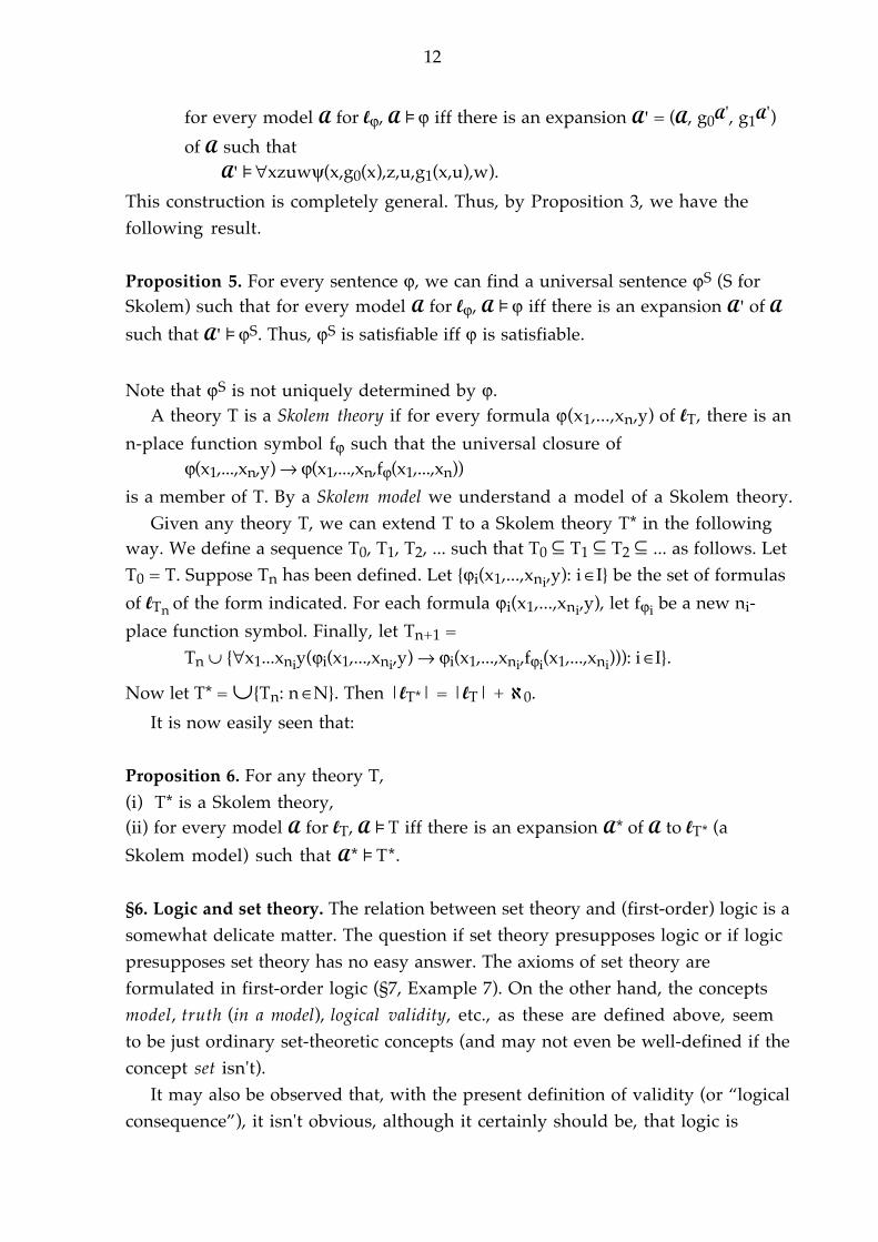
for every model A for lϕ, A[ϕ iff there is an expansion A' = (A, g0A', g1A')

of A such thatA'[∀xzuwψ(x,g0(x),z,u,g1(x,u),w).

This construction is completely general. Thus, by Proposition 3, we have thefollowing result.

Proposition 5. For every sentence ϕ, we can find a universal sentence ϕS (S forSkolem) such that for every model A for lϕ, A[ϕ iff there is an expansion A' of A

such that A'[ϕS. Thus, ϕS is satisfiable iff ϕ is satisfiable.

Note that ϕS is not uniquely determined by ϕ.A theory T is a Skolem theory if for every formula ϕ(x1,...,xn,y) of lT, there is an

n-place function symbol fϕ such that the universal closure ofϕ(x1,...,xn,y) → ϕ(x1,...,xn,fϕ(x1,...,xn))

is a member of T. By a Skolem model we understand a model of a Skolem theory.Given any theory T, we can extend T to a Skolem theory T* in the following

way. We define a sequence T0, T1, T2, ... such that T0 ˘ T1 ˘ T2 ˘ ... as follows. LetT0 = T. Suppose Tn has been defined. Let {ϕi(x1,...,xni,y): iŒI} be the set of formulas

of lTn of the form indicated. For each formula ϕi(x1,...,xni,y), let fϕi be a new ni-

place function symbol. Finally, let Tn+1 =Tn ∪ {∀x1...xniy(ϕi(x1,...,xni,y) → ϕi(x1,...,xni,fϕi(x1,...,xni))): iŒI}.

Now let T* = ∪{Tn: nŒN}. Then |lT*| = |lT| + ℵ0.

It is now easily seen that:

Proposition 6. For any theory T,(i) T* is a Skolem theory,(ii) for every model A for lT, A[T iff there is an expansion A* of A to lT* (a

Skolem model) such that A*[T*.

§6. Logic and set theory. The relation between set theory and (first-order) logic is asomewhat delicate matter. The question if set theory presupposes logic or if logicpresupposes set theory has no easy answer. The axioms of set theory areformulated in first-order logic (§7, Example 7). On the other hand, the conceptsmodel, truth (in a model), logical validity, etc., as these are defined above, seemto be just ordinary set-theoretic concepts (and may not even be well-defined if theconcept set isn't).

It may also be observed that, with the present definition of validity (or “logicalconsequence”), it isn't obvious, although it certainly should be, that logic is

13

applicable in set theory, where the domain (range of the variables) is a properclass and not a set. In fact, we haven't even defined “truth” (in a model) in thiscase. But although our definition of validity may not be intensionally correct, i.e.,yield the right concept, it is extensionally correct (for L1), i.e., the right sentences

are characterized as valid (see Chapter 2, §9).

§7. Some first-order theories. This section consists of a list of examples that willlater (in Chapter 3) be used to illustrate model-theoretic concepts and theorems.In these examples we often leave out the initial universal quantifiers of axioms.

Example 1. Linear orderings. Let ≤ be a two-place predicate. The theory LO of(reflexive) linear (or simple) orderings is the set of the following sentences(axioms).

∀xyz(x ≤ y ∧ y ≤ z → x ≤ z),∀xyz(x ≤ y ∧ y ≤ x → x = y),∀x(x ≤ x),∀xy(x ≤ y ∨ y ≤ x).

We write x < y for x ≤ y ∧ x ≠ y. The theory DiLO of discrete linear orderings with

no endpoints is LO plus:∀x∃y(x < y ∧ ∀z(x < z → y ≤ z)),∀x∃y(y < x ∧ ∀z(z < x → z ≤ y)).

Let Z be the set of integers and ≤ the usual ordering of Z. (Z, ≤) is a model of DiLO.The theory DeLO of dense linear orderings without endpoints is obtained

from LO by adding:∀xy(x < y → ∃z(x < z ∧ z < y)),∀x∃y(x < y),∀x∃y(y < x).

Let Ra and Re be the sets of rational and real numbers, respectively. Let ≤ be theusual ordering of Ra (Re). Then (Ra, ≤) and (Re, ≤) are models of DeLO. �

Example 2. The successor function. Let S be a one-place function symbol and 0a constant. Let Sn(x) be defined by: S0(x) := x, Sn+1(x) := S(Sn(x)). SF, the theory ofthe successor function, is then the set of the following sentences.

∀xy(S(x) = S(y) → x = y),∀x(S(x) ≠ 0),∀x(Sn+1 (x) ≠ x), nŒN,∀x(x ≠ 0 → ∃y(x = S(y))).

(N, S, 0), where S is the successor function, S(i) = i+1, is a model of SF. �Example 3. Boolean algebras. Let ∩, ∪ be two-place function symbols, * a one-

place function symbol, and 0, 1 individual constants. We write x* for *(x). Thetheory BA of Boolean algebras has the following members (axioms).

14

x ∩ y = y ∩ x, x ∪ y = y ∪ x,(x ∩ y) ∩ z = x ∩ (y ∩ z), (x ∪ y) ∪ z = x ∪ (y ∪ z),x ∩ (y ∪ z) = (x ∩ y) ∪ (x ∩ z), x ∪ (y ∩ z) = (x ∪ y) ∩ (x ∪ z),x ∩ x = x, x ∪ x = x,x ∩ (x ∪ y) = x, x ∪ (x ∩ y) = x,(x ∩ y)* = x* ∪ y*, (x ∪ y)* = x* ∩ y*,x** = x, 0 ≠ 1,x ∪ 0 = x, x ∩ 0 = 0,x ∩ 1 = x, x ∪ 1 = 1,x ∩ x* = 0, x ∪ x* = 1.

In BA we can define a partial ordering ≤ by letting x ≤ y be x ∩ y = x or,equivalently, x ∪ y = y.

Let At(x) (x is an atom) be the formulax ≠ 0 ∧ ∀z(z ≤ x → z = 0 ∨ z = x).

Adding∀x(x ≠ 0 → ∃y(At(y) ∧ y ≤ x))

to BA we get the theory AtBA of atomic Boolean algebras. Finite Boolean algebrasare atomic.

Let X be any set, let S(X) be the set of subsets of X. Then (S(X), ∩, ∪, *, Ø, X),where ∩, ∪ are understood as usual and Y* = X – Y, is an atomic Boolean algebra.

The theory NoAtBA of atomless Boolean algebras is obtained from BA byadding

∀x¬At(x).Let PF be the set of formulas of propositional logic (in the variables p0, p1, p2,

...). For every FŒPF, let [F] = {GŒPF: G ↔ F is a tautology}. Let [F] ∩ [G] = [F ∧ G],[F] ∪ [G] = [F ∨ G], [F]* = [¬F], 0PF = [⊥], and 1PF = [H], where H is any tautology.Finally, let [PF] = {[F]: FŒPF}. Then ([PF], ∩, ∪, *, 0PF, 1PF) is an atomless Boolean

algebra. �Example 4. Groups. Let + be a two-place function symbol, – a one-place

function symbol, and 0 an individual constant. The theory G of groups has theaxioms:

(x + y) + z = x + (y + z),x + –x = 0, –x + x = 0,x + 0 = x, 0 + x = x.

In view of the first axiom, the associative law, parentheses in terms may beomitted.

The theory AG of Abelian groups has the additional axiomx + y = y + x.

15

For every n > 0, let nx be and x + x +...+ x, with n occurrences of x. A group G istorsion-free if the sentences

∀x(nx = 0 → x = 0)are true in G. G is divisible if the sentences

∀x∃y(x = ny)are true in G:

Let TAG and DTAG be the theories of torsion-free and divisible torsion-freeAbelian groups, respectively.

(Re, +, –, 0), where Re is the set of real numbers and +, – (a one-placefunction), and 0 are understood as usual, are models of DTAG. Another exampleis (Re2, +', –', 0'), where ¤r,s% +'¤r',s'% = ¤r+s,r'+s'%, –'¤r,s% = ¤–r,–s%, and 0' =¤0,0%. �

Example 5. Fields. Let +, . be two-place function symbols and let 0, 1 beindividual constants. The axioms of the theory of fields are as follows.

x + y = y + x, (x + y) + z = x + (y + z),

x . y = y . x, (x . y) . z = x . (y . z),

x . (y + z) = (x . y) + (x . z),x + 0 = x, ∃y(x + y = 0),

x . 1 = x, x . y = 0 → x = 0 ∨ y = 0,

0 ≠ 1, x ≠ 0 → ∃y(x . y = 1).

Since + and . are associative, we may omit parentheses in terms in the usual way.For every natural number n > 0, let nx be the term x + x + x +...+ x and let xn be

the term x . x ..... x, in both cases with n occurrences of x. A field F is ofcharacteristic p if p1 = 0 is true in F. F is of characteristic 0 if n1 ≠ 0 is true in F forall n > 0. Every field is of characteristic p, for some prime p, or of characteristic 0.

(Ra, +, ., 0, 1) and (Re, +, ., 0, 1) are fields of characteristic 0.F is an algebraically closed field if every polynomial with coefficients in F has a

zero in F, i.e., the following sentences (one for each n > 0) are true in F.

(1n) xn ≠ 0 → ∃y(xn. yn + xn–1. yn–1 +...+ x1. y + x0 = 0).

The complex numbers form an algebraically closed field of characteristic 0(Fundamental Theorem of Algebra).

Let ACF (ACF(p), where p is 0 or a prime) be the theory of algebraically closedfields (of characteristic p).

F = (F', ≤) is an ordered field if F' is a field and ≤ is a linear ordering of F and

the following axioms are true in F:x ≤ y → x + z ≤ y + z,

16

x ≤ y ∧ 0 ≤ z → x . z ≤ y . z.An ordered field F is real closed if (1n), for n odd, and the following axiom are

true in F:0 ≤ x → ∃y(x = y2).

The real numbers form a real closed ordered field. Let RCOF be the theory ofreal closed ordered fields. �

Example 6. Arithmetic. The axioms of (first-order) Peano Arithmetic, PA, areas follows:

S(x) = S(y) → x = y, S(x) ≠ 0,x + 0 = x, x + S(y) = S(x + y),

x . 0 = 0, x . S(y) = (x . y) + x,ϕ(0) ∧ ∀x(ϕ(x) → ϕ(S(x))) → ∀xϕ(x),

where ϕ(x) is any formula of the language {+, ., S, 0} of arithmetic and maycontain free variables other than x. This axiom scheme is the first-orderapproximation of the full (second-order) axiom of induction.

Q ((Raphael) Robinson’s Arithmetic) is the theory obtained from PA bydropping the induction scheme and adding the axiom

x ≠ 0 → ∃y(x = S(y)).Exponentiation and other common number-theoretic functions and concepts

can be defined in terms of + and . . �Example 7. Set theory. We shall not give the details of the axiomatization of

ZF(C), Zermelo-Fraenkel set theory (with the axiom of choice), since these detailsare lengthy and irrelevant for our present purposes. What is relevant, however,is the fact that ZFC is formalized in L1 (lZF = {∈}). This is particularly interesting,

since (practically all of) classical (non-constructive) mathematics can bedeveloped in ZFC. In this sense, all the logic you need in mathematics is first-order logic. �

Notes for Chapter 1. The definitions of satisfaction and truth in a model is due toTarski (1935), (1952), but these concepts were quite well understoodindependently of Tarski's definitions (see, for example, Hilbert, Ackermann(1928)). That set theory can, and should, be formalized in first-order logic waspointed out by Skolem (1922).

17

2. COMPLETENESS

Having defined the concept logical consequence,[, our next task is to developsystematic methods by means of which statements of the form Φ[ϕ can beestablished. To this end we introduce four different formal methods (calculi) eachwith its advantages and disadvantages. As the reader will notice, the first three ofthese, FH, GS, and ND (§§ 1, 3, 6) are based on the same logical intuitions. But theformal representations of these intuitions are different leading to formal calculiwith quite different properties.

Given a formal logical calculus LC it is natural to ask if it can be improved, ifthere are cases of logical validity or consequence that cannot be established bymeans of LC. For example, there may be some (simple) rule of derivation that hasbeen overlooked or some very complicated rule(s) may be required or, worse, itmay turn out that no finite set of rules will be sufficient. Given the vast variety ofdeductive arguments and methods of proof in the mathematical literature, thereis prima facie no reason at all to rule out these possibilities. But, remarkably, forL1 (though not for certain (natural) extensions of L1; see Chapter 5) this is not the

case.A logical calculus LC for L1 is complete if a sentence ϕ can be shown to follow

from a set Φ of sentences, using only the means available in LC, whenever Φ[ϕ.The calculi presented here are complete in this sense (Corollary 1 and Theorems7, 10, 11).

It should be observed that these calculi are defined in purely syntactical terms,with no reference to the semantical interpretation of the formulas involved(though, of course, with this semantical interpretation in mind). This is essential:our ambition is to lay bare all the logical intuitions that go into the constructionof a derivation by means of the method in question.

In this chapter l is an arbitary but fixed language. Thus, in what follows,“formula”, “term”, etc. mean formula of l, term of l, etc. We assume that lcontains an “inexhaustible” set of individual constants (parameters).

§1. Frege-Hilbert-type systems. The Frege-Hilbert system FH (for l) has thefollowing logical axioms. In these axioms ϕ(x) is any formula with the one freevariable x, ψ is any sentence, and t is any closed term.A1. All closed propositional tautologies,A2. ∀xϕ(x) → ϕ(t),A3. ∀x(ψ → ϕ(x)) → (ψ → ∀xϕ(x)),A4. ϕ(t) → ∃xϕ(x),A5. ∀x(ϕ(x) → ψ) → (∃xϕ(x) → ψ).

18

The identity axioms of FH are the universal closures of the followingformulas.I1. x = x,I2. x = y → y = x,I3. x = y ∧ y = z → x = z,I4. x1 = y1 ∧...∧ xn = yn → (ϕ(x1,...,xn) → ϕ(y1,...,yn)),I5. x1 = y1 ∧...∧ xn = yn → t(x1,...,xn) = t(y1,...,yn).

An axiom of FH is either a logical axiom or an identity axiom.There are two rules of inference (derivation).

R1. Modus Ponens: ϕ, ϕ → ψ/ψ.R2. Universal Generalization: ϕ(c)/∀xϕ(x).

In these axioms and rules we can restrict ourselves to sentences, since freevariables can always be replaced by parameters.

Let Φ be a set of sentences. A (logical) derivation in FH of ϕ from Φ is asequence ϕ0, ϕ1,..., ϕn of sentences such that ϕn := ϕ and for every k ≤ n either (i) ϕk

is an axiom of FH or (ii) ϕkŒΦ or (iii) there are i, j < k such that ϕj := ϕi → ϕk (R1)or (iv) ϕk := ∀xψ(x) and for some i < k, ϕi := ψ(c), where c does not occur in Φ, ψ(x)(R2). ϕ is derivable (in FH) from Φ, in symbols Φ©FHϕ, if there is a derivation of ϕ

from Φ. If Φ is the empty set, we (may) drop all references to Φ. If we think of Φ asa theory, we shall sometimes say “proof in Φ” and “provable in Φ” instead of“derivation from Φ“ and “derivable from Φ”.

Among the identity axioms only I1 and I4 for n = 1 and ϕ an atomic formulaare essential; given these, I2, I3, I4, I5 can be derived.

In this section and the next we write© for©FH.

In what follows we shall frequently (implicitly) use the following:

Lemma 1. (a) If ϕ is an axiom or ϕ∈Φ, then Φ©ϕ.(b) If Φ© ϕ, there is a finite subset Φ' of Φ such that Φ'© ϕ.

(c) If Φ©ϕ and Φ ˘ Ψ, then Ψ©ϕ.

Proof. (a) is trivial. (b) This is clear, since every derivation (from Φ) is finite.(c) This, too, is clear except for the slight complication that a derivation of ϕ

from Φ may not be a derivation of ϕ from Ψ: the applications of R2 may no longerbe legal, since the constant c involved, although it doesn't occur in Φ, may occurin Ψ. But such constants can always be replaced by constants not occurring in Ψ. �

Example 1. The sequence of the following formulas (sentences) is a derivation of(*) ∀x¬ϕ(x) → ¬∃xϕ(x)

19

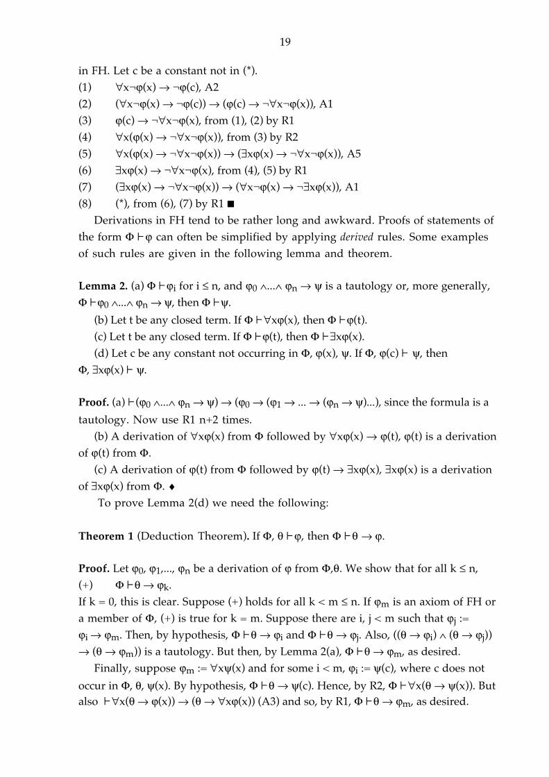
in FH. Let c be a constant not in (*).(1) ∀x¬ϕ(x) → ¬ϕ(c), A2(2) (∀x¬ϕ(x) → ¬ϕ(c)) → (ϕ(c) → ¬∀x¬ϕ(x)), A1(3) ϕ(c) → ¬∀x¬ϕ(x), from (1), (2) by R1(4) ∀x(ϕ(x) → ¬∀x¬ϕ(x)), from (3) by R2(5) ∀x(ϕ(x) → ¬∀x¬ϕ(x)) → (∃xϕ(x) → ¬∀x¬ϕ(x)), A5(6) ∃xϕ(x) → ¬∀x¬ϕ(x), from (4), (5) by R1(7) (∃xϕ(x) → ¬∀x¬ϕ(x)) → (∀x¬ϕ(x) → ¬∃xϕ(x)), A1(8) (*), from (6), (7) by R1 �

Derivations in FH tend to be rather long and awkward. Proofs of statements ofthe form Φ©ϕ can often be simplified by applying derived rules. Some examplesof such rules are given in the following lemma and theorem.

Lemma 2. (a) Φ©ϕi for i ≤ n, and ϕ0 ∧...∧ ϕn → ψ is a tautology or, more generally,Φ©ϕ0 ∧...∧ ϕn → ψ, then Φ©ψ.

(b) Let t be any closed term. If Φ©∀xϕ(x), then Φ©ϕ(t).(c) Let t be any closed term. If Φ©ϕ(t), then Φ©∃xϕ(x).(d) Let c be any constant not occurring in Φ, ϕ(x), ψ. If Φ, ϕ(c)© ψ, then

Φ, ∃xϕ(x)© ψ.

Proof. (a)©(ϕ0 ∧...∧ ϕn → ψ) → (ϕ0 → (ϕ1 → ... → (ϕn → ψ)...), since the formula is a

tautology. Now use R1 n+2 times.(b) A derivation of ∀xϕ(x) from Φ followed by ∀xϕ(x) → ϕ(t), ϕ(t) is a derivation

of ϕ(t) from Φ.(c) A derivation of ϕ(t) from Φ followed by ϕ(t) → ∃xϕ(x), ∃xϕ(x) is a derivation

of ∃xϕ(x) from Φ. ♦ To prove Lemma 2(d) we need the following:

Theorem 1 (Deduction Theorem). If Φ, θ©ϕ, then Φ©θ → ϕ.

Proof. Let ϕ0, ϕ1,..., ϕn be a derivation of ϕ from Φ,θ. We show that for all k ≤ n,(+) Φ©θ → ϕk.If k = 0, this is clear. Suppose (+) holds for all k < m ≤ n. If ϕm is an axiom of FH ora member of Φ, (+) is true for k = m. Suppose there are i, j < m such that ϕj :=ϕi → ϕm. Then, by hypothesis, Φ©θ → ϕi and Φ©θ → ϕj. Also, ((θ → ϕi) ∧ (θ → ϕj))→ (θ → ϕm)) is a tautology. But then, by Lemma 2(a), Φ©θ → ϕm, as desired.

Finally, suppose ϕm := ∀xψ(x) and for some i < m, ϕi := ψ(c), where c does not

occur in Φ, θ, ψ(x). By hypothesis, Φ©θ → ψ(c). Hence, by R2, Φ©∀x(θ → ψ(x)). Butalso ©∀x(θ → ϕ(x)) → (θ → ∀xϕ(x)) (A3) and so, by R1, Φ©θ → ϕm, as desired.

20

Thus, we have shown that (+) holds for all k ≤ n and so, in particular, fork = n; in other words, Φ©θ → ϕ, as desired. �Proof of Lemma 2(d). Suppose Φ, ϕ(c)© ψ. Then, by Theorem 1, Φ© ϕ(c) → ψ.Hence, by R2, Φ© ∀x(ϕ(x) → ψ). But©∀x(ϕ(x) → ψ) → (∃xϕ(x) → ψ) (A5). And so,by R1 (twice), Φ, ∃xϕ(x)© ψ. �

Example 2. That (*) in Example 1 is derivable can now be shown as follows.(1) © ∀x¬ϕ(x) → ¬ϕ(c), A2(2) © ϕ(c) → ¬∀x¬ϕ(x), (1), Lemma 2(a)(3) ϕ(c)© ¬∀x¬ϕ(x), (2), R1(4) ∃xϕ(x)© ¬∀x¬ϕ(x), (3), Lemma 2(d)(5) © (*), (4), Theorem 1 �

Example 3. As a second example we show that(**) ©∀x(ϕ(x) → ψ(x)) → (∃xϕ(x) → ∃xψ(x))is derivable. Let c be a new constant.(1) ∀x(ϕ(x) → ψ(x))© (ϕ(c) → ψ(c)), Lemma 2(b)(2) ∀x(ϕ(x) → ψ(x)), ϕ(c)© ψ(c), (1), R1(3) ∀x(ϕ(x) → ψ(x)), ϕ(c)© ∃xψ(x), (2), Lemma 2(c)(4) ∀x(ϕ(x) → ψ(x)), ∃xϕ(x)© ∃xψ(x), (3), Lemma 2(d)(5) © (**), (4), Theorem 1 (twice).

§2. Soundness and completeness of FH. Of course, we want our formal system tobe sound in the sense that Φ©ϕ implies that Φ[ϕ. And this is easily established.

Theorem 2 (Soundness of FH). If Φ©ϕ, then Φ[ϕ.

Proof. Let ϕ0, ϕ1,..., ϕn be a derivation of ϕ from Φ. We show that for all k ≤ n,(*) Φ[ϕk.This holds for k = 0, since ϕ0 is either an axiom of FH or a member of Φ. Suppose(*) holds for all k < m ≤ n. We want to show that it holds for k = m. If ϕm is anaxiom of FH or a member of Φ, this is true. Suppose there are i, j < m such that ϕj

:= ϕi → ϕm. Then, since, by hypothesis, Φ[ϕi and Φ[ϕj, it follows that Φ[ϕm.Finally, suppose ϕm := ∀xψ(x) and for some i < m, ϕi := ψ(c), where c does notoccur in Φ, ψ(x). By hypothesis, Φ[ψ(c). It follows that Φ[ϕm.

Thus, we have shown that (*) holds for all k ≤ n and so, in particular, for k = n;in other words, Φ[ϕ, as desired. �

It may seem that this proof is circular, that we have “shown” that certainlogical principles are valid by appealing to those very principles (plus

21

mathematical induction). But that is not correct. What we have shown is not thatthe logical principles are valid, that is obvious, or almost, but that our formalrendering of these principles is correct.

A set Φ of sentences is consistent (in FH) if there is no sentence ϕ such thatΦ©ϕ and Φ©¬ϕ. By Lemma 1(b), if every finite subset of Φ is consistent, so is Φ.

We are now going to prove the following:

Theorem 3. If Φ is consistent, then Φ has a model.

Corollary 1 (Gödel-Henkin Completeness Theorem). If Φ[ϕ, then Φ©ϕ.

The problem in proving Theorem 3 is that, given only that Φ is consistent, wehave no idea what a model of Φ may look like. The main idea of the proof is toovercome this difficulty by defining a set Φ* of sentences such that (i) Φ ˘ Φ*, (ii)Φ* is consistent, lΦ* = lΦ ∪ C, where C is a set of constants (Lemma 10), (iii) Φ* can

be used in a natural way to define a model A (the canonical model for Φ*, seebelow), and, finally, (iv) it can be shown for every sentence ϕ of lΦ* (by induction

on the length of ϕ), that A[ϕ iff ϕŒΦ* (proof of Lemma 13). It follows that A[Φ*and so A[Φ, as desired.

Lemma 3. The following conditions are equivalent.(i) Φ is inconsistent.(ii) Φ©⊥.(iii) For every sentence ϕ, Φ©ϕ.

Proof. (i) ⇒ (ii). Let ϕ be such that Φ©ϕ and Φ©¬ϕ. Φ© ϕ ∧ ¬ϕ → ⊥. But then, byLemma 2(a), Φ©⊥.

(ii) ⇒ (iii). Suppose Φ©⊥. Let ϕ be any sentence. Φ©⊥ → ϕ and so Φ©ϕ.(iii) ⇒ (i). Asume (iii). Let θ be any sentence. Then Φ©θ ∧ ¬θ. It follows that

Φ©θ and Φ©¬θ and so Φ is inconsistent. �

Lemma 4. (a) The following conditions are equivalent.(i) Φ© ϕ.(ii) Φ ∪ {¬ϕ} is inconsistent.

(b) The following conditions are equivalent.(iii) Φ© ¬ϕ.(iv) Φ ∪ {ϕ} is inconsistent.

Proof. (a) (i) ⇒ (ii). Suppose Φ©ϕ. Then Φ ∪ {¬ϕ}©ϕ. Also, clearly, Φ ∪ {¬ϕ}©¬ϕ.

22

Thus, Φ ∪ {¬ϕ} is inconsistent.(ii) ⇒ (i). Suppose Φ ∪ {¬ϕ} is inconsistent. Then, by Lemma 3, Φ ∪ {¬ϕ}©⊥.

By the Deduction Theorem, it follows that Φ©¬ϕ → ⊥ and so Φ©ϕ.The proof of (b) is similar. �

Proof of Corollary 1. Suppose Φ£ϕ. Then, by Lemma 4, Φ ∪ {¬ϕ} is consistent. Itfollows, by Theorem 3, that Φ ∪ {¬ϕ} has a model A. But then A[Φ and A]ϕ andso Φ]ϕ. �

Theorem 3 can also easily be derived from Corollary 1.A set Φ of sentences is explicitly complete if for every sentence, either ϕŒΦ or

¬ϕŒΦ. (This sense of “complete” is, of course, different from that in which FH iscomplete.)

The following lemma is clear.

Lemma 5. If Φ is explicitly complete and consistent, then Φ©ϕ iff ϕŒΦ.

Lemma 6. (a) If Φ is consistent, then for every sentence ϕ, either Φ ∪ {ϕ} orΦ ∪ {¬ϕ} is consistent.

(b) Suppose X is a set of consistent sets of sentences and for all Φ0, Φ1ŒX, either

Φ0 ˘ Φ1 or Φ1 ˘ Φ0. Then ∪X is consistent.

Proof. (a) Suppose Φ ∪ {ϕ} and Φ ∪ {¬ϕ} are inconsistent. Then Φ ∪ {ϕ}©⊥ andΦ ∪ {¬ϕ}©⊥. By the Deduction Theorem, Φ©ϕ → ⊥ and Φ©¬ϕ → ⊥. It follows thatΦ©⊥ and so Φ is inconsistent.

(b) Every finite subset of ∪X is included in some ΦŒX. �

Lemma 7 (Lindenbaum's Theorem). If Φ is consistent, there is a set Ψ of sentencesof lΦ such that Φ ˘ Ψ and Ψ is explicitly complete and consistent.

Proof. Countable case. We first give a proof under the additional assumption thatlΦ is countable and so the set of sentences is denumerable. Let ϕ0, ϕ1, ϕ2, ... be anenumeration of the sentences of lΦ. Let Φn be defined as follows: Φ0 = Φ,

Φn+1 = Φn ∪ {ϕn} if Φn ∪ {ϕn} is consistent, = Φn ∪ {¬ϕn} otherwise.

Let Ψ = ∪{Φn: nŒN}. Ψ is explicitly complete. If Φn is consistent, by Lemma 6(a),

so is Φn+1. Thus all Φn are consistent. But then, by Lemma 6(b), Ψ is consistent. ♦If lΦ is uncountable, there is no enumeration of the sentences of lΦ as above

23

and it becomes necessary to use set theory in one form or another: ordinals anddefinition and proof by transfinite induction or some set-theoretical principlesuch as the following result.

Let X be a set of subsets of a given set. A chain in X is then a subset of X whichis linearly ordered by ˘. A maximal element of X is a member of X which is not aproper subset of a member of X.

Zorn's Lemma (special case). Let X be a set of subsets of a given set such that for

every chain Y ˘ X, ∪YŒX. Then X has a maximal element.

Proof of Lemma 7 (concluded). Uncountable case. Let X be the set of sets Θ ofsentences of lΦ such that Φ ˘ Θ and Θ is consistent. By Lemma 6(b), the union of achain in X is consistent and so is a member of X. Hence, by Zorn's Lemma, X has amaximal element Ψ. Ψ is consistent. Suppose Ψ is not explicitly complete. Let ψbe such that ψ, ¬ψœΨ. Then, Ψ being maximal, Ψ ∪ {ψ} and Ψ ∪ {¬ψ} areinconsistent, contrary to Lemma 6(a). Thus, Ψ is explicitly complete. �

Let C be a set of constants. A set Φ of sentences is witness-complete (withrespect to C) if for every member of Φ of the form ∃xϕ(x), there is a constant c (inC), a witness to ∃xϕ(x), such that ϕ(c)ŒΦ. We shall now show that everyconsistent set Φ can be extended to an explicitly complete witness-completeconsistent set.

Lemma 8. Suppose Φ is consistent and ∃xϕ(x)ŒΦ. Let c be a constant not in lΦ.Then Φ ∪ {ϕ(c)} is consistent.

Proof. Suppose Φ ∪ {ϕ(c)} is inconsistent. Then Φ©¬ϕ(c) and so, by R2, Φ©

∀x¬ϕ(x). But, trivially, Φ© ∃xϕ(x). Also we have already shown that© ∀x¬ϕ(x)→¬∃xϕ(x) (Examples 1, 2). It follows that Φ©¬∃xϕ(x). And so Φ is inconsistent,contrary to assumption. �

Lemma 9. Suppose Φ is consistent. Let {ϕi(xi): iŒI} be the set of formulas ϕ(x) such

that ∃xϕ(x)ŒΦ. Let {ci: iŒI} be a set of constants not in lΦ. Then Φ ∪ {ϕi(ci): iŒI} is

consistent.

Proof. It is sufficient to show that for every finite subset J of I, Φ ∪ {ϕi(ci): iŒJ} is

consistent. But this follows by repeated applications of Lemma 8. �

24

Lemma 10. For every consistent set Φ, there is an explicitly complete witness-complete consistent set Φ* such that Φ ˘ Φ*.

Proof. We define sets of sentences Φn, Ψn and sets Cn of constants as follows. LetΦ0 = Φ and C0 = Ø. Suppose Cn and Φn have been defined and Φn is a consistent set

of sentences of lΦ ∪ Cn. Let {ϕi(xi): iŒIn} be the set of formulas ϕ(x) of lΦ ∪ Cn such

that ∃xϕ(x)ŒΦn. Let {ci,n: iŒIn} be a set of constants not in Cn. Let Cn+1 = Cn ∪{ci,n: iŒI} and Ψn = Φn ∪ {ϕi,n(ci,n): iŒIn}. Then, by Lemma 9, Ψn is consistent.

Finally, by Lemma 7, there is an explicitly complete extension Φn+1 of Ψn in

lΦ ∪ Cn+1.

Now let

Φ* = ∪{Φn: nŒN}

and C = ∪{Cn: nŒN}. Then Φ* is explicitly complete and witness-complete (with

respect to C). Finally, by Lemma 6(b), Φ* is consistent, as desired. �Suppose Ψ, a set of sentences of lΦ ∪ C, is consistent, explicitly complete, and

witness-complete with respect to C. Let t be a closed term of lΦ ∪ C. Since© ∃x(t = x), and so ∃x(t = x)ŒΨ, there is a cŒC such that t = cŒΨ.

We define the relation ~ on C by:c ~ d iff c = dŒΨ.

By I1, I2, I3, and since Ψ is explicitly complete and consistent, ~ is an equivalence

relation. Let [c] be the equivalence class of c. Let [C] be the set of such equivalenceclasses.

We now define the canonical model A for Ψ as follows. A = [C]. cA = [c] for cŒC.If dŒlΦ, there is a cŒC such that c = dŒΨ. Let dA = [c]. If PŒlΦ is an n-placepredicate, let

PA = {¤[c1],...,[cn]%: c1,...,cnŒC & Pc1...cnŒΨ}. By I4, if [c1] = [c1'],..., [cn] = [cn'], then Pc1...cnŒΨ iff Pc1'...cn'ŒΨ. And so

¤[c1],...,[cn]%ŒPA iff Pc1...cnŒΨ.Finally, let fŒlΦ be an n-place function symbol. Suppose c1,...,cnŒC. There is a

cŒC such that f(c1,...,cn) = cŒΨ. LetfA([c1],...,[cn]) = [c].

By I5, this is a proper definition of a function fA; in other words,if [c1] = [c1'],..., [cn] = [cn'], then fA([c1],...,[cn]) = fA([c1'],...,[cn']).

Lemma 11. Suppose t is a closed term of lΦ ∪ C and let cŒC be such that t = cŒΨ.Then tA = [c].

25

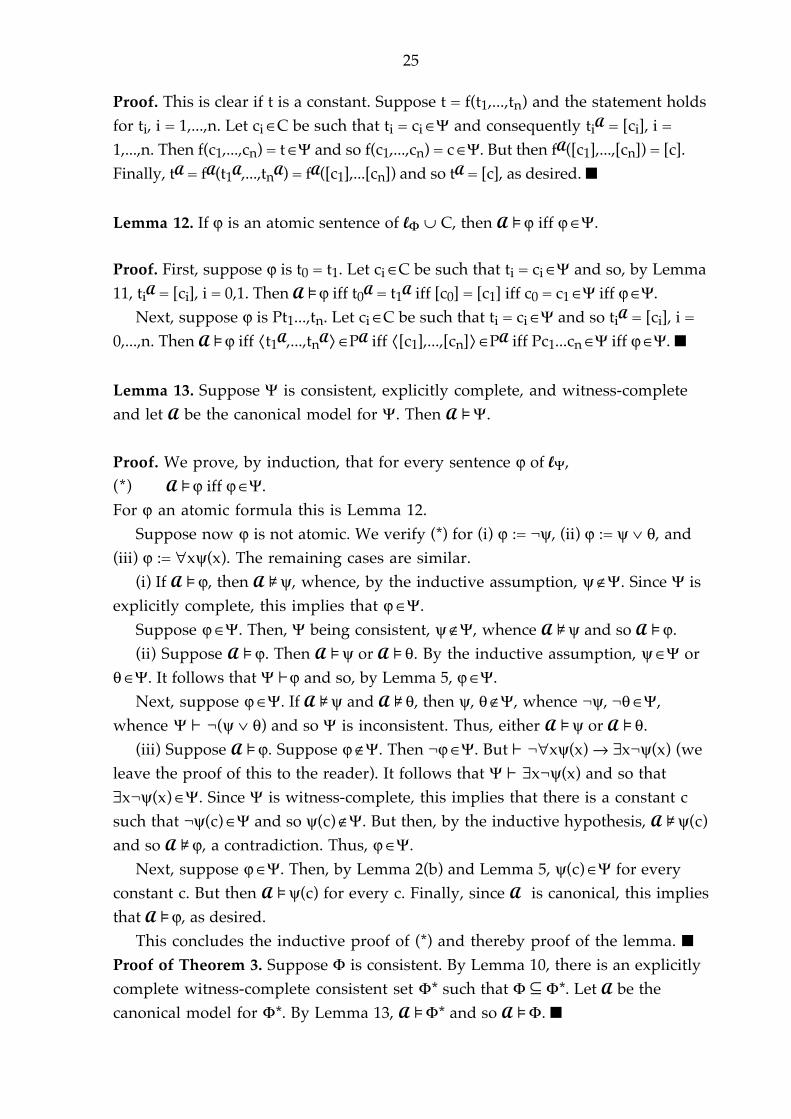
Proof. This is clear if t is a constant. Suppose t = f(t1,...,tn) and the statement holdsfor ti, i = 1,...,n. Let ciŒC be such that ti = ciŒΨ and consequently tiA = [ci], i =1,...,n. Then f(c1,...,cn) = tŒΨ and so f(c1,...,cn) = cŒΨ. But then fA([c1],...,[cn]) = [c].Finally, tA = fA(t1A,...,tnA) = fA([c1],...[cn]) and so tA = [c], as desired. �

Lemma 12. If ϕ is an atomic sentence of lΦ ∪ C, then A[ϕ iff ϕŒΨ.

Proof. First, suppose ϕ is t0 = t1. Let ciŒC be such that ti = ciŒΨ and so, by Lemma11, tiA = [ci], i = 0,1. Then A[ϕ iff t0A = t1A iff [c0] = [c1] iff c0 = c1ŒΨ iff ϕŒΨ.

Next, suppose ϕ is Pt1...,tn. Let ciŒC be such that ti = ciŒΨ and so tiA = [ci], i =0,...,n. Then A[ϕ iff ¤t1A,...,tnA%ŒPA iff ¤[c1],...,[cn]%ŒPA iff Pc1...cnŒΨ iff ϕŒΨ. �

Lemma 13. Suppose Ψ is consistent, explicitly complete, and witness-completeand let A be the canonical model for Ψ. Then A[Ψ.

Proof. We prove, by induction, that for every sentence ϕ of lΨ,(*) A[ϕ iff ϕŒΨ.For ϕ an atomic formula this is Lemma 12.

Suppose now ϕ is not atomic. We verify (*) for (i) ϕ := ¬ψ, (ii) ϕ := ψ ∨ θ, and(iii) ϕ := ∀xψ(x). The remaining cases are similar.

(i) If A[ϕ, then A]ψ, whence, by the inductive assumption, ψœΨ. Since Ψ isexplicitly complete, this implies that ϕŒΨ.

Suppose ϕŒΨ. Then, Ψ being consistent, ψœΨ, whence A]ψ and so A[ϕ.(ii) Suppose A[ϕ. Then A[ψ or A[θ. By the inductive assumption, ψŒΨ or

θŒΨ. It follows that Ψ©ϕ and so, by Lemma 5, ϕŒΨ.Next, suppose ϕŒΨ. If A]ψ and A]θ, then ψ, θœΨ, whence ¬ψ, ¬θŒΨ,

whence Ψ© ¬(ψ ∨ θ) and so Ψ is inconsistent. Thus, either A[ψ or A[θ.(iii) Suppose A[ϕ. Suppose ϕœΨ. Then ¬ϕŒΨ. But© ¬∀xψ(x) → ∃x¬ψ(x) (we

leave the proof of this to the reader). It follows that Ψ© ∃x¬ψ(x) and so that∃x¬ψ(x)ŒΨ. Since Ψ is witness-complete, this implies that there is a constant csuch that ¬ψ(c)ŒΨ and so ψ(c)œΨ. But then, by the inductive hypothesis, A]ψ(c)and so A]ϕ, a contradiction. Thus, ϕŒΨ.

Next, suppose ϕŒΨ. Then, by Lemma 2(b) and Lemma 5, ψ(c)ŒΨ for everyconstant c. But then A[ψ(c) for every c. Finally, since A is canonical, this impliesthat A[ϕ, as desired.

This concludes the inductive proof of (*) and thereby proof of the lemma. �Proof of Theorem 3. Suppose Φ is consistent. By Lemma 10, there is an explicitlycomplete witness-complete consistent set Φ* such that Φ ˘ Φ*. Let A be thecanonical model for Φ*. By Lemma 13, A[Φ* and so A[Φ. �

26

Let ϕ be any valid sentence. By Corollary 1, there is then a derivation d of ϕ(from the empty set) in FH. It is then natural to ask if we can impose an upperbound on the length |d| of d, i.e., the number of occurrences of symbols in d, interms of the length |ϕ| of ϕ in some (any) reasonably interesting way. Similarquestions can be asked about the calculi GS and ND presented below. Thesequestions will be answered in Chapter 4.

§3. A Gentzen-type sequent calculus. The main disadvantage of FH, in additionto the fact that it is quite unnatural, is that given that a formula ϕ is derivable inFH, we know next to nothing about its derivation: we know nothing about whichformulas occur in the derivation nor how complicated they are. If ϕ has beenderived by R1 from ψ and ψ → ϕ, there is no way of working “backwards” toreconstruct ψ from ϕ or even estimate the complexity of ψ. In this section weintroduce a logical calculus, GS, for which we know a great deal about theformulas occurring in any derivation (see, for example, the Subformula Property,below). On the other hand many obvious logical principles such as ModusPonens (rule R1 of FH) and (the more general) Cut Rule (p. 30) are now difficultto derive.

In this section and the next two sections we assume, for simplicity, that thereare no function symbols. Also, the presence of = causes certain technicalproblems, of limited interest in themselves, and so we restrict ourselves toformulas not containing =.

We now add a new symbol ⇒ (implies) to the formal language. Γ, ∆ are finite

sets (not sequences) of sentences (not containing ⇒). Expressions such as Γ ⇒ ∆are called sequents. (Γ and/or ∆ may be empty. If Γ is empty, we may write ⇒ ∆ forΓ ⇒ ∆ and similarly if ∆ or both Γ and ∆ are empty.) The intended intuitiveinterpretation of Γ ⇒ ∆ is that the conjunction of Γ implies the disjunction of ∆.

(∧Ø is true and ∨Ø is false.) We write A[Γ ⇒ ∆ to mean that if A[Γ, then A[ϕ

for some ϕŒ∆. Γ ⇒ ∆ is (logically) valid,[Γ ⇒ ∆, if A[Γ ⇒ ∆ for every A. Theunion of Γ and ∆ will be written as Γ, ∆. Γ, ϕ is Γ, {ϕ}.

Axioms of GS: All sequents of the form Γ, ϕ ⇒ ∆, ϕ.Rules of inference of GS:

(⇒¬) Γ , ϕ ⇒ ∆ (¬⇒) Γ ⇒ ∆ , ϕ Γ ⇒ ∆, ¬ϕ Γ, ¬ϕ ⇒ ∆

(⇒∧) Γ ⇒ ∆ , ϕ 0 Γ ⇒ ∆ , ϕ 1 (∧⇒) Γ , ϕ 0 , ϕ 1 ⇒ ∆ Γ ⇒ ∆, ϕ0 ∧ ϕ1 Γ, ϕ0 ∧ ϕ1 ⇒ ∆

(⇒∨) Γ ⇒ ∆ , ϕ 0 , ϕ 1 (∨⇒) Γ , ϕ 0 ⇒ ∆ Γ , ϕ 1 ⇒ ∆ Γ ⇒ ∆, ϕ0 ∨ ϕ1 Γ, ϕ0 ∨ ϕ1 ⇒ ∆

27

(⇒→) Γ , ϕ ⇒ ∆ , ψ (→⇒) Γ ⇒ ∆ , ϕ Γ , ψ ⇒ ∆ Γ ⇒ ∆, ϕ → ψ Γ, ϕ → ψ ⇒ ∆

(⇒∃) Γ ⇒ ∆ , ψ (c) (∃⇒) Γ , ψ (c) ⇒ ∆ Γ ⇒ ∆, ∃xψ(x) Γ, ∃xψ(x) ⇒ ∆

(⇒∀) Γ ⇒ ∆ , ψ (c) (∀⇒) Γ , ψ (c) ⇒ ∆ Γ ⇒ ∆, ∀xψ(x) Γ, ∀xψ(x) ⇒ ∆

In (∃⇒) and (⇒∀) the individual constant c must not occur below the line.In the conclusion of instances of each of these rules a logical constant is

introduced. The formula containing this constant is called the principal formula

of the inference; and the formula or formulas shown explicitly in the premise(s)its active formula(s).

It may be observed that, unlike the rules of FH and those of ND (below), therules of GS are inversely valid in the sense that if the conclusion is valid, thenthe pemise(s) is (are) valid. Another important difference is that in GS, but not inFH or ND, there are explicit rules for each of the propositional connectives.

Derivations in GS take the form of trees in a quite obvious way. We use ©GS to

denote derivability in GS. In this and the following two §§ we write © for ©GS.

Example 4. ©∀x(Fx ∨ Gx) ⇒ ∀xFx, ∃x(¬Fx ∧ Gx), Ga, Fa ⇒ Fa (⇒¬) Ga ⇒ Fa, ¬Fa Ga ⇒ Fa, Ga (⇒∧)

Fa ⇒ Fa, ¬Fa ∧ Ga Ga ⇒ Fa, ¬Fa ∧ Ga (∨⇒) Fa ∨ Ga ⇒ Fa, ¬Fa ∧ Ga (⇒∃) Fa ∨ Ga ⇒ Fa, ∃ x(¬Fx ∧ Gx) (∀⇒) ∀ x(Fx ∨ Gx) ⇒ Fa, ∃ x(¬Fx ∧ Gx) (⇒∀)∀x(Fx ∨ Gx) ⇒ ∀xFx, ∃x(¬Fx ∧ Gx) �

Example 5. Suppose ψ is a sentence.© ψ → ∃xϕ(x) ⇒ ∀x¬ϕ(x) → ¬ψ.

Let a be a new constant. ϕ (a) ⇒ ϕ (a), ¬ ψ (¬⇒) ϕ (a), ¬ ϕ (a) ⇒ ¬ ψ (∀⇒)

ψ , ∀ x¬ ϕ (x), ⇒ ψ (⇒¬) ϕ (a), ∀ x¬ ϕ (x) ⇒ ¬ ψ (∃⇒) ∀ x¬ ϕ (x), ⇒ ψ , ¬ ψ (⇒→) ∃ x ϕ (x), ∀ x¬ ϕ (x) ⇒ ¬ ψ (⇒→) ⇒ ψ , ∀ x¬ ϕ (x) → ¬ ψ ∃ x ϕ (x) ⇒ ∀ x¬ ϕ (x) → ¬ ψ (→⇒)

ψ → ∃xϕ(x) ⇒ ∀x¬ϕ(x) → ¬ψ �

28

A derivation of a sequent Γ ⇒ ∆ in GS may be though of as (the inverse of) anabortive attempt to construct a counterexample to Γ ⇒ ∆, i.e., a model A such thatA[Γ and A]ψ for every ψŒ∆. Proceeding from the bottom up we try to make allthe formulas occurring to the left of ⇒ true (in A) and all the formulas occurringto the right of ⇒ false along at least one branch. And we give up only if someformula occurs both to the left and to the right of ⇒ (as in the axioms of GS). Thiscan always be done in such a way that the result is either a counterexample toΓ ⇒ ∆ or a derivation of Γ ⇒ ∆ in GS (see Examples 1, 2 in Appendix 1 and theproof of Theorem 7, below).

As is easily checked, GS has the:

Subformula Property. Every formula occurring in the derivation of a sequent S isa subformula or a formula occurring in S.

Here “subformula” is used in the somewhat technical sense: ϕ is a subformula ofψ if ϕ is a subformula of ψ in the usual sense or is obtained from such a formulaby replacing free variables by individual constants.

From the Subformula Property it follows at once that any logical constantoccurring in a derivation of S occurs in S.

It may be observed thatif©Γ ⇒ ∆, Γ ˘ Γ', and ∆ ˘ ∆', then©Γ' ⇒ ∆'.

This is true, since the constants occurring in instances of (∃⇒) and (⇒∀) canalways be assumed not to occur in Γ', ∆'.

Certain obviously sound principles (derived rules of inference) are ratherdifficult to establish for GS. The prime example is the so-called Cut Rule:(Cut) Γ , ϕ ⇒ ∆ Γ ⇒ ∆ , ϕ

Γ ⇒ ∆In fact, the result that (Cut) is a derived rule of GS, the so-called Cut EliminationTheorem, is one of the major results of the proof theory of L1. With (Cut) added

the system no longer has the Subformula Property (see Appendix 1, Example 1).The system GS= is obtained from GS by adding the sequents Γ ⇒ ∆, c = c, where

c is any individual constant, as new axioms and the rules of inference: Γ , ϕ (c) ⇒ ∆ , ψ (c)

Γ, ϕ(c'), c = c' [c' = c] ⇒ ∆, ψ(c')Theorems 4(a) and 7, below, can be extended to GS=.

For completeness we have stated the inference rules for →. But in the next twosectionswe do not regard → as a primitive symbol partly because the rules ofderivation for → cause problems similar to those caused by the ¬-rules (see

29

below). Instead we think of ϕ → ψ as an abbreviation of ¬ϕ ∨ ψ. The →-rules arethen derived rules. But we do retain all of ∧, ∨, ∀, ∃, since we want to be able towrite formulas in n.n.f.

§4. Two applications. In this § we give two applications, Theorems 4 and 5, below,of GS or, more accurately, three closely related systems GSa, GS⊥, and GS*.

Let GSa be obtained from GS by taking as axioms only those axioms of GS inwhich all formulas are atomic. Let GS⊥ be obtained from GS by adding theconstant ⊥ to the language and all sequents Γ, ⊥ ⇒ ∆ to the set of axioms. Finally,let GS* be obtained from GSa by replacing the rules (⇒∧) and (∨⇒) by:(⇒∧)* Γ 0 ⇒ ∆ 0 , ϕ 0 Γ 1 ⇒ ∆ 1 , ϕ 1 and (∨⇒)* Γ 0 , ϕ 0 ⇒ ∆ 0 Γ 1 , ϕ 1 ⇒ ∆ 1

Γ0, Γ1 ⇒ ∆0, ∆1, ϕ0 ∧ ϕ1 Γ0, Γ1, ϕ0 ∨ ϕ1 ⇒ ∆0, ∆1

We denote derivability in GSa, GS⊥, GS* by©a,©⊥,©*, respectively.Clearly, GSa, GS⊥, GS* have the Subformula Property.

Lemma 14. The systems GSa, GS⊥, GS* are equivalent to GS for sequents of GS.

Proof. Obviously,©a Γ ⇒ ∆ implies© Γ ⇒ ∆. To prove the inverse implication itis sufficient to show that all axioms of GS are derivable in GSa. If(1) Γ, ϕ ⇒ ∆, ϕis an axiom of GS which is not an axiom of GSa, either some member ψ of Γ or ∆is not atomic or ϕ is not atomic. In both cases the non-atomic formula can bereplaced by one or two simpler formulas, i.e., formulas containing fewer logicalconstants. If, for example, ¬θ is a member of Γ, we replace (1) by Γ – {¬θ}, ϕ ⇒∆, θ, ϕ from which (1) can be derived by (¬⇒). If ∀xψ(x) is a member of ∆, let c be anew constant and replace (1) by Γ, ϕ ⇒ ∆ – {∀xψ(x)}, ψ(c), ϕ from which (1) can bederived by (⇒∀). The remaining cases are similar.

If ϕ is not atomic, for example, ϕ := ϕ0 ∧ ϕ1 or ϕ := ∃xψ(x), then ϕ can be replaced

by simpler formulas as follows: Γ , ϕ 0 , ϕ 1 ⇒ ∆ , ϕ 0 (∧⇒) Γ , ϕ 0 , ϕ 1 ⇒ ∆ , ϕ 1 (∧⇒) Γ , ψ (c) ⇒ ∆ , ψ (c) (⇒∃) Γ , ϕ 0 ∧ ϕ 1 ⇒ ∆ , ϕ 0 Γ , ϕ 0 ∧ ϕ 1 ⇒ ∆ , ϕ (⇒∧) Γ , ψ (c) ⇒ ∆ , ∃ x ψ (x) (∃⇒)

Γ, ϕ0 ∧ ϕ1 ⇒ ∆, ϕ0 ∧ ϕ1 Γ, ∃xψ(x) ⇒ ∆, ∃xψ(x)

The remaining cases are similar. In this way axioms of GS containing non-atomicformulas can be replaced by axioms of GSa.

Obviously,© S implies©⊥ S. If S is a sequent of GS and©⊥ S, then, by theSubformula Property for GS⊥, ⊥ does not occur in the derivation D of S in GS⊥.But then D is a derivation in GS and so© S.

© S implies©a S and, obviously,©a S implies©* S. Thus,© S implies©* S.

30

We have observed that if© Γ' ⇒ ∆', Γ' ˘ Γ'', and ∆' ˘ ∆'', then©Γ'' ⇒ ∆''. Itfollows that (⇒∧)* and (∨⇒)* are derived rules of GS. Thus,©* S implies© S. �

As an application of GS⊥ we shall now prove a (sufficiently general) specialcase of the following interpolation theorem.

χ is an interpolant for Γ ⇒ ∆ in GS (GS⊥) if χ is a sentence of lΓ ∩ l∆ such that© Γ ⇒ χ and© χ ⇒ ∆ (©⊥ Γ ⇒ χ and©⊥ χ ⇒ ∆).

Note that if l contains no predicates, the set of formulas of l in GS is empty.Thus, if lΓ ∩ l∆ contains no predicates, there is no interpolant for Γ ⇒ ∆ in GS andthe only possible interpolants for Γ ⇒ ∆ in are propositional combinations of ⊥’s.

Theorem 4. (a) (Interpolation Theorem for GS⊥). If©⊥ Γ ⇒ ∆, there is aninterpolant for Γ ⇒ ∆ in GS⊥. (b) If©⊥ Γ ⇒ ∆ and Γ, ∆ have no predicates in common, then©⊥ Γ ⇒ or©⊥ ⇒ ∆.

The proof if this result is quite long and will only be sketched. But we shall proveTheorem 4 assuming that the members of Γ, ∆ are in n.n.f.

A rule of inference preserves the existence of interpolants if whenever there isan interpolant for an instance of the premise of the rule or there are interpolantsfor the premises of an instance of the rule, there is one for its conclusion.

If Γ ⇒ ∆ is an axiom, then, trivially, there is an interpolant for Γ ⇒ ∆.Moreover, we have the following:

Lemma 15. The existence of interpolants is preserved under the ∧-, ∨-, ∃-, ∀-rules.

Proof. We verify this in three cases; the remaining cases are similar. First,consider an instance of (∨⇒):

Γ , ϕ 0 ⇒ ∆ Γ , ϕ 1 ⇒ ∆ Γ, ϕ0 ∨ ϕ1 ⇒ ∆

By assumption there are interpolants χi for Γ, ϕi ⇒ ∆, i = 0, 1. Then, by (∨⇒) and(⇒∨),©⊥ Γ, ϕ0 ∨ ϕ1 ⇒ χ0 ∨ χ1 and, by (∨⇒),©⊥χ0 ∨ χ1 ⇒ ∆. Every predicate inχ0 ∨ χ1 occurs in Γ, ϕ0 ∨ ϕ1 and in ∆. χ0 ∨ χ1 is an interpolant for Γ, ϕ0 ∨ ϕ1 ⇒ ∆.

Next, consider an instance of (⇒∃): Γ ⇒ ∆ , ϕ (c) Γ ⇒ ∆, ∃xϕ(x)

By hypothesis there is a formula χ(x) not containing c such that χ(c) is aninterpolant for Γ ⇒ ∆, ϕ(c).

There are then three cases.Case 1. c occurs in both Γ and ∆, ∃xϕ(x). χ(c) is an interpolant for Γ ⇒ ∆, ∃xϕ(x).

31

Case 2. c does not occur in Γ. Then c does not occur in χ(c) and so χ(x) is asentence χ. χ is an interpolant for Γ ⇒ ∆, ∃xϕ(x).

Case 3. c does not occur in ∆, ∃xϕ(x). Then, by (⇒∃),©⊥ Γ ⇒ ∃xχ(x) and, by (∃⇒),©⊥ ∃xχ(x) ⇒ ∆, ∃xϕ(x). Thus, ∃xχ(x) is an interpolant for Γ ⇒ ∆, ∃xϕ(x).

Finally, consider an instance of (∃⇒): Γ , ϕ (c) ⇒ ∆ Γ, ∃xϕ(x) ⇒ ∆

By hypothesis there is an interpolant χ for Γ, ϕ(c) ⇒ ∆. By (∃⇒),©⊥ Γ, ∃xϕ(x) ⇒ χ.Thus, χ is an interpolant for Γ, ∃xϕ(x) ⇒ ∆. �

Note that we may now infer the interpolation theorem for positive formulas,i.e., formulas with no logical constants other than ∧, ∨, ∃, ∀.

The ¬-rules and →-rules, too, preserve the existence of interpolants; theproblem is that this is not so obvious. To deal with this difficulty one has toprove the following more complicated lemma. Let ¬Γ = {¬ϕ: ϕŒ Γ}.

Lemma 16. If©⊥ Γ0, Γ1 ⇒ ∆0, ∆1, there is an interpolant for Γ0, ¬∆0 ⇒ ¬Γ1, ∆1.

We shall not give the (rather long) proof of this lemma.To deal with the ¬-rules for formulas in n.n.f. we use the following:

Lemma 17. In any derivation (in GS⊥), any instance of a non-¬-rule Rimmediately followed by a ¬-inference, whose active formula is not the principalformula of the instance of R, can be replaced by one instance or two side-by-sideinstances of the ¬-rule followed by an instance of R.

Proof. We consider just two special cases; the other cases are similar. If R is (⇒∧)and the ¬-rule is (¬⇒), the relevant part of the derivation looks as follows: Γ ⇒ ∆ , ϕ , ψ 0 Γ ⇒ ∆ , ϕ , ψ 1 This can be replaced by:

Γ ⇒ ∆ , ϕ, ψ 0 ∧ ψ 1 Γ ⇒ ∆ , ϕ , ψ 0 Γ ⇒ ∆ , ϕ , ψ 1 Γ, ¬ϕ ⇒ ∆, ψ0 ∧ ψ1 Γ , ¬ ϕ ⇒ ∆ , ψ 0 Γ , ¬ ϕ ⇒ ∆ , ψ 1

Γ, ¬ϕ ⇒ ∆, ψ0 ∧ ψ1

Next, suppose R is (⇒∀) and the ¬-rule is (⇒¬). The relevant part of thederivation then looks as follows:

Γ , ϕ ⇒ ∆ , ψ (c) This can be replaced by: Γ , ϕ ⇒ ∆ , ψ (c) Γ , ϕ ⇒ ∆ , ∀ x ψ (x) Γ ⇒ ∆ , ψ (c), ¬ ϕ Γ ⇒ ∆, ∀xψ(x), ¬ϕ Γ ⇒ ∆, ∀xψ(x), ¬ϕ �

Proof of Theorem 4 for n.n.f. formulas. (a) Suppose©⊥ Γ ⇒ ∆, where themembers of Γ, ∆ are in n.n.f. Let D be a derivation of Γ ⇒ ∆ in GS⊥. By the

32

Subformula Property for GS⊥, the active formula of every instance of a ¬-rule inD is atomic and so cannot be the principal formula of a non-¬-rule. Hence, byLemma 17, there is a derivation D' of Γ ⇒ ∆ in which no non-¬-inference is

followed by a ¬-inference.In D' every branch begins with a number, possibly zero, of ¬-inferences and

below these there is no ¬-inference. If a sequent is an axiom or obtained from anaxiom by ¬-inferences, it is of the form Γ’, ϕ ⇒ ∆’, ϕ or Γ’, ϕ, ¬ϕ ⇒ ∆’ or Γ’ ⇒ ∆’, ϕ,¬ϕ or Γ’, ⊥ ⇒ ∆’ or Γ’ ⇒ ∆’, ¬⊥. (All formulas are in n.n.f.) In these cases ϕ, ⊥, ¬⊥,⊥, ¬⊥, respectively, are interpolants for Γ’ ⇒ ∆’. Now use Lemma 15.

(b) Let us say that Γ ⇒ ∆ is hyperderivable if either©⊥ Γ ⇒ or©⊥ ⇒ ∆. Let D bea derivation of Γ ⇒ ∆ in which no non-¬-inference is followed by a ¬-inference.Let Γ’ ⇒ ∆’ be an upermost sequent in D, possibly Γ ⇒ ∆, below which there is no¬-inference. Then Γ’, ∆’ have no predicate in common. For if they do, theantecedent and consequent of every sequent below Γ’ ⇒ ∆’ will have a predicatein common. It follows that Γ’ ⇒ ∆’ is either an axiom Γ’’, ⊥ ⇒ ∆’’ for ⊥ or not anaxiom and so is the conclusion of a ¬-inference. In the latter case Γ’ ⇒ ∆’ is of theform Γ’’, ϕ, ¬ϕ ⇒ ∆’’ or Γ’’ ⇒ ∆’’, ϕ, ¬ϕ or Γ’’ ⇒ ∆’’, ¬⊥. In all these cases Γ’ ⇒ ∆’ ishyperderivable. Furthermore, if the premise (premises) of a non-¬-inference is(are) hyperderivable, so is its conclusion. Thus, Γ ⇒ ∆ is hyperderivable. �

Even if ⊥ does not occur in Γ ⇒ ∆ and Γ, ∆ have a predicate in common, theinterpolant χ for Γ ⇒ ∆ defined in the above proof of Theorem 4 for n.n.f.formulas may contain ⊥. But such occurrences of ⊥ can easily be eliminated (fromthe respective derivations). Thus, we have:

Corollary 2. (a) (Interpolation Theorem for GS). If© Γ ⇒ ∆ and lΓ and l∆ have apredicate in common, there is an interpolant for Γ ⇒ ∆ in GS.

(b) If© Γ ⇒ ∆ and lΓ ∩ l∆ = Ø, then© Γ ⇒ or© ⇒ ∆.

Our second application, of GS*, concerns derivations of those valid sequents inwhich all formulas are in prenex normal form.

A derivation D in GS* is in PQ normal form if all propositional inferencesprecede all quantificational inferences and the sequents appearing inpropositional inferences are quantifier-free. This implies that there is a sequent Sin D such that all inferences above S are propositional and all inferences at orbelow S are quantificational. Since the quantificational rules are one-premiserules, it follows that the sequents below S are linearly ordered. Thus, a derivationin PQ normal form in GS is of a particularly simple and perspicuous form. Thederivation in Example 4, above, is in PQ normal form.

33

Theorem 5. Suppose S is derivable in GS and all formulas occurring in S areprenex formulas. There is then a derivation of S in GS in PQ normal form.

A derivation D (in GS or GS*) is said to be strict if for every instance of (∃⇒) in D,the constant c does not occur anywhere in D except above the conclusion of thatinstance; and similarly for instances of (⇒∀).

Lemma 18. For every derivation in GS (GS*), there is a strict derivation in GS(GS*) of the same sequent.

Proof. Let D be any derivation in GS or GS*. For every instance Γ , ϕ (c) ⇒ ∆ Γ, ∃xϕ(x) ⇒ ∆

of (∃⇒) in D, let d be a constant not occurring in D and replace c in the formulasabove Γ, ∃xϕ(x) ⇒ ∆ by d. Similarly for instances of (⇒∀). Repeating thisoperation we eventually obtain a strict derivation. �

Lemma 19. In a strict derivation in GS*, an instance of a quantifier rule R, withprincipal formula ϕ, immediately followed by an instance of a propositional ruleR’ in which ϕ is not an active formula, can be replaced by an instance of R’immediately followed by an instance of R. The resulting derivation is strict.

Proof. If R’ is a ¬-rule, this is Lemma 17. We consider two more special cases; theremaining cases are similar.

(i) R is (∃⇒) and R’ is (∧⇒). The relevant part of the derivation then looks asfollows:

Γ , ψ 0 , ψ 1 , ϕ (c) ⇒ ∆ This can be replaced by: Γ , ψ 0 , ψ 1 , ϕ (c) ⇒ ∆ Γ , ψ 0 , ψ 1 , ∃ x ϕ (x) ⇒ ∆ Γ , ψ 0 ∧ ψ 1 , ϕ (c) ⇒ ∆ Γ, ψ0 ∧ ψ1, ∃xϕ(x) ⇒ ∆ Γ, ψ0 ∧ ψ1, ∃xϕ(x) ⇒ ∆

(ii) R is (⇒∀) and R’ is (∨⇒)*. The relevant part of the derivation is then: Γ 1 , ψ 1 ⇒ ∆ 1 , ϕ (c)

Γ 0 , ψ 0 ⇒ ∆ 0 Γ 1 , ψ 1 ⇒ ∆ 1 , ∀ x ϕ (x) (∨⇒)*Γ0, Γ1, ψ0 ∨ ψ1 ⇒ ∆0, ∆1, ∀xϕ(x)

This can be replaced by: Γ 0 , ψ 0 ⇒ ∆ 0 Γ 1 , ψ 1 ⇒ ∆ 1 , ϕ (c) (∨⇒)* Γ 0 , Γ 1 , ψ 0 ∨ ψ 1 ⇒ ∆ 0 , ∆ 1 , ϕ (c) Γ0, Γ1, ψ0 ∨ ψ1 ⇒ ∆0, ∆1, ∀xϕ(x)

34

It is then clear that the istances of (∃⇒) and (⇒∀) in the new derivations are legaland that these derivations are strict. �

Lemma 20. If D is a derivation (in GS or GS*) of a sequent S such that all formulasin S are prenex (including quantifier-free formulas), then no formula containinga quantifier is an active formula of a propositional inference in D.

Proof. By the Subformula Property, ever formula occurring in D is prenex.Moreover, if an active formula of a propositional inference contains a quantifier,then the principal formula of that inference is not prenex. �Proof of Theorem 5. Suppose all formulas occurring in S are prenex formulas. ByLemmas 14 and 18, there is a strict derivation D’ of S in GS*. By Lemma 20, noprincipal formula of a quantifier inference in D’ is an active formula of apropositional inference. But then, by repeated application of Lemma 19, there is a(strict) derivation D’’ of S in GS* in PQ normal form.

Finally, it the propositional part of D’’ can be replaced by a (quantifier-free)derivation in GS. The result is a derivation of S in GS in PQ normal form. �

Corollary 3. Suppose©⇒ ϕ and ϕ is in prenex normal form. There is then a finite

set ∆ of quantifier-free sentences such that ∨∆ is a propositional tautology and

⇒ ϕ can be obtained from ⇒ ∆ by applying the rules (⇒∃) and (⇒∀).

§5. Soundness and completeness of GS. If Γ ⇒ ∆ is an axiom of GS, thenobviously [Γ ⇒ ∆. It is also easy to verify that for any instance of a rule ofderivation (of GS), if the premise (premises) is (are) valid, so is the conclusion.Thus, we get:

Theorem 6 (Soundness of GS). If©Γ ⇒ ∆, then[Γ ⇒ ∆.

Next, we prove the following completeness theorem. The proof is similar to thatof Theorem 3, but because of the special nature of the rules of derivation of GS,we have to proceed somewhat more carefully.

Theorem 7 (Completeness Theorem for GS). If[Γ ⇒ ∆, then©Γ ⇒ ∆.

It is easy to derive the completeness theorem for GS with the Cut Rule from thatfor FH. But then to obtain completeness of GS we need the Cut EliminationTheorem. For this reason we shall instead give a direct proof of the completeness

35

of GS. From this it follows, of course, that the Cut Rule is redundant.We now begin the proof of Theorem 7. Let Const(Φ) be the set of constants

occurring in Φ if this set is ≠ Ø; if not, let Const(Φ) = {d}, where d is an arbitaryfixed constant. (This is to make sure that Const(Φ) ≠ Ø.) Let (Σ,Π) be any orderedpair of (possibly infinite) sets of formulas. We shall say that a formula ϕ requires

attention in (Σ,Π) if one of the following conditions is satisfied:(i) ϕ := ¬ψ, ϕŒΣ, and ψœΠ,(ii) ϕ := ¬ψ, ϕŒΠ, and ψœΣ,(iii) ϕ := ψ0 ∧ ψ1, ϕŒΣ, and ψ0œΣ or ψ1œΣ,

(iv) ϕ := ψ0 ∧ ψ1, ϕŒΠ, ψ0œΠ and ψ1œΠ,

(v) ϕ := ψ0 ∨ ψ1, ϕŒΣ, ψ0œΣ and ψ1œΣ,

(vi) ϕ := ψ0 ∨ ψ1, ϕŒΠ, and ψ0œΠ or ψ1œΠ,

(vii) ϕ := ∀xψ(x), ϕŒΣ, and there is a constant cŒConst(Σ∪Π) such that ψ(c)œΣ,(viii) ϕ := ∀xψ(x), ϕŒΠ, and there is no constant c such that ψ(c)ŒΠ,(ix) ϕ := ∃xψ(x), ϕŒΣ, and there is no constant c such that ψ(c)ŒΣ,(x) ϕ := ∃xψ(x), ϕŒΠ, and there is a constant cŒConst(Σ∪Π) such that ψ(c)œΠ.

(Φ,Ψ) is closed if no formula requires attention in (Φ,Ψ). A is a model of (Φ,Ψ),A[(Φ,Ψ), if A[Φ and A]ψ for every ψœΨ. Thus,[Γ ⇒ ∆ iff there is no model of(Γ,∆).

Suppose (Φ,Ψ) is closed and Φ and Ψ are disjoint. A is a canonical model for

(Φ,Ψ) if the following conditions are satisfied. Let C = Const(Φ∪Ψ). Then C ≠ Ø.A = C, cA = c. If P is an n-place predicate and c1,...,cnŒC, let

PA = {¤c1,...,cn%: Pc1...cnŒΦ}.Note that it may happen that Pc1...cn, ¬Pc1...cnœΦ ∪ Ψ. In fact, you need to appeal

to the Cut Rule to show that Φ, Ψ can always be defined in such a way that thisdoes not happen. If it does, we may, but need not, put ¤c1,...,cn% in PA.

Lemma 21. Suppose (Φ,Ψ) is closed and Φ and Ψ are disjoint. Let A be a canonicalmodel for (Φ,Ψ). Then A[(Φ,Ψ).

Proof. We show, by induction, that for every ϕ,(1) if ϕŒΦ, then A[ϕ,(2) if ϕŒΨ, then A]ϕ.This is clear for atomic ϕ. The inductive steps are similar to those of the proof ofLemma 13. We consider only the cases, (i) ϕ := ¬ψ, (ii) ϕ := ∀xψ(x); the remainingcases are similar.

(i) Suppose ϕŒΦ. Since ϕ does not require attention in (Φ,Ψ), it follows thatψŒΨ. But then, by the inductive assumption, A]ψ and so A[ϕ.

36

Next, suppose ϕŒΨ. Since ϕ does not require attention in (Φ,Ψ), it follows thatψŒΦ. But then, by the inductive assumption, A[ψ and so A]ϕ.

(ii) Suppose ϕŒΦ. Since ϕ does not require attention in (Φ,Ψ), ψ(c)ŒΦ for everycŒC. It follows, by the inductive assumption, that A[ψ(c) for every cŒC. Since A= C, this implies that A[ϕ.

Suppose ϕŒΨ. Since ϕ does not require attention in (Φ,Ψ), there is a constant csuch that ψ(c)ŒΨ. But then, by the inductive assumption, A]ψ(c) and so A]ϕ. �

Lemma 22. If£Γ ⇒ ∆, there is a closed pair (Φ,Ψ) such that Γ ˘ Φ, ∆ ˘ Ψ, and Φand Ψ are disjoint.

Proof. Let C be a denumerable set of individual constants not in lΓ∪∆. Let ϕ0, ϕ1,ϕ2, ... be an enumeration of the sentences of lΓ∪∆ ∪ C. “First” in “first sentence”,

below, refers to this enumeration.We define sequents Γn ⇒ ∆n, n = 0, 1, 2, ..., as follows. Let Γ0 ⇒ ∆0 be Γ ⇒ ∆.

Now, suppose Γn ⇒ ∆n has been defined and£Γn ⇒ ∆n. (This, of course, implies

that Γn and ∆n are disjoint.) There are then two cases. (a) (Γn,∆n) is closed. In this

case the construction terminates. (b) Otherwise. In this case one of the sentencesrequiring attention in (Γn,∆n) receives attention at n but exactly which one is not

important as long as(*) for all n and ϕ, if ϕ requires attention in (Γn,∆n), then ϕ receives attention

at some n' ≥ n.

The reason there is a slight problem is that, in view of (vii), (x), some sentencesmay require attention many, even infinitely many, times. (If at n a sentencecontaining a new constant is added to Γn or ∆n, every sentence ∀xψ(x) in Γn+1 and

every sentence ∃xψ(x) in ∆n+1 requires attention in (Γn+1,∆n+1).) But (*) can be

ensured in many different ways. For example, if there is a sentence requiringattention by (vii) or (x), let ϕ be the first such sentence; and if there is no suchsentence, let ϕ be the first sentence, if there is one, requiring attention (for someother reason).

Let ϕ be the sentence which receives attention at n. Γn+1 and ∆n+1 are then

defined as follows. Suppose Σ = Γn and Π = ∆n. Then

if (i) applies, let Γn+1 = Γn and ∆n+1 = ∆n, ψ,

if (ii) applies, let Γn+1 = Γn, ψ and ∆n+1 = ∆n,

if (iii) applies, let Γn+1 = Γn, ψ0, ψ1 and ∆n+1 = ∆n,

if (iv) applies, then (since£Γn ⇒ ∆n)£Γn ⇒ ∆n, ψi for i = 0 or i = 1; let j be an i

for which this holds and let Γn+1 = Γn and ∆n+1 = ∆n, ψj,

if (v) applies, then (since£Γn ⇒ ∆n)£Γn, ψi ⇒ ∆n for i = 0 or i = 1; let j be an i

37

for which this holds and let Γn+1 = Γn, ψj and ∆n+1 = ∆n,

if (vi) applies, let Γn+1 = Γn and ∆n+1 = ∆n, ψ0, ψ1,

if (vii) applies, let c be any constant in Const(Γn∪∆ n) such that ψ(c)œΓn and let

Γn+1 = Γn, ψ(c) and ∆n+1 = ∆n,

if (viii) applies, let c be any constant not in (Γn,∆n) and let Γn+1 = Γn, ∆n+1 =

∆n, ψ(c),

if (ix) applies, let c be a constant not in (Γn,∆n), let Γn+1 = Γn, ψ(c), and ∆n+1 = ∆n,

if (x) applies, let c be any constant in Const(Γn∪∆ n) such that ψ(c)œ∆n and let

Γn+1 = Γn and ∆n+1 = ∆n, ψ(c).

It now follows that£Γn+1 ⇒ ∆n+1. This is clear in cases (iv) and (v) and holds

in the other cases, too, since then Γ n+1 ⇒ ∆ n+1

Γn ⇒ ∆n

is an instance of a rule of derivation. Now, let Φ and Ψ be defined as follows. If case (a) applies at n, let Φ = Γn and Ψ

= ∆n, if (b) applies at every n, let Φ = ∪{Γn: nŒN} and Ψ = ∪{∆n: nŒN}. Then Γ ˘

Φ, ∆ ˘ Ψ, Φ and Ψ are disjoint, and, by (*), (Φ,Ψ) is closed. �Proof of Theorem 7. Let Γ ⇒ ∆ be any sequent. Suppose£Γ ⇒ ∆. By Lemma 22,there is a closed pair (Φ,Ψ) such that Γ ˘ Φ, ∆ ˘ Ψ, and Φ and Ψ are disjoint. ByLemma 21, there is a model A such that A[(Φ,Ψ). It follows that A[(Γ,∆) andso]Γ ⇒ ∆, as desired. �

Theorem 7 implies the Cut Elimination Theorem.From Theorem 7 and Corollary 3 we get:

Corollary 4. Suppose ϕ is valid and in prenex normal form. There is then a finite

set ∆ of quantifier-free sentences such that ∨∆ is a propositional tautology and

⇒ ϕ can be obtained from ⇒ ∆ by applying the rules (⇒∃) and (⇒∀).

Combining Theorem 7 with the form of the interpolation theorem alreadyproved and Proposition 1.2 we get the following interpolation theorem (restrictedto sentences not containing = nor any function symbols).

Theorem 8 (Craig's Interpolation Theorem). Let ϕ, ψ be any two sentences. If[ϕ → ψ, there is a sentence χ such that every nonlogical constant occurring in χoccurs in both ϕ and ψ,[ϕ → χ and[χ → ψ.

38

§6. Natural Deduction. The formal systems FH and GS are quite artificial and donot correspond at all closely to the way we tend to reason intuitively. In thissection we present a formal system, a version ND of natural deduction – there areother versions – which does not suffer from this disadvantage. On the otherhand it is more complicated than FH and GS.

There are no axioms but nine rules of derivation: P (premise rule), PL (rule ofpropositional logic), US (universal specification), UG (universal generalization),ES (existential specification), EG (existential generalization), Cond(conditionalization), and two rules I and I* of identity.

The rules UG and ES embody the same ways of reasoning as the axioms A3and A5 and rule R2 of FH and the rules (⇒∀) and (∃⇒) of GS. The rule Cond iswhat in the present context corresponds to the Deduction Theorem for FH andthe rule (⇒→) of GS. (The reader may want to look at the derivations below andin Appendix 1 to see how the various rules are applied in practice.)

A derivation is a (finite) column of lines:(D) (1) ϕ1 X1R1Y1

(2) ϕ2 X2R2Y2

..............................(n) ϕn XnRnYn

Each Rk is one of the above rules of derivation, ϕk is obtained from {ϕm: mŒXk}by applying Rk, and {ϕm: mŒYk} is the set of premises in (D), introduced byapplying P, on which ϕk “depends”, i.e., from which ϕk has been derived, exceptwhen Rk is P, in which case Xk = Ø and Yk = {k}. Thus, (D) is a derivation of ϕn

from {ϕm: mŒYn}.

(D) is a derivation in ND if one of the following conditions (i) – (ix) aresatisfied:(i) Rk is P and Xk = Ø and Yk = {k} (on any line you may introduce a new premise;

it “depends” only on itself),(ii) Rk is PL and ϕk is a tautological consequence of ϕk1,...,ϕkm, where ki < k for i ≤

m, Xk = {k1,...,km}, and Yk = Yk1 ∪...∪ Ykm,

(iii) Rk is US and there are m < k, ψ(x), and a closed term t such that ϕm is ∀xψ(x), ϕk is ψ(t), Xk = {m}, and Yk = Ym,

(iv) Rk is UG and there are m < k, ψ(x), and c such that ϕk is ∀xψ(x), ϕm is ψ(c), c does not occur in ϕk nor in any premise of ϕm, Xk = {m}, and Yk = Ym,

(v) Rk is EG, there are m < k, ψ(x), and a closed term t such that ϕk is ∃xψ(x), ϕm is ψ(t), Xk = {m}, and Yk = Ym,

(vi) Rk is ES and there are m, p, q < k, ψ(x), and c such that ϕm is ϕk, ϕp is ∃xψ(x), ϕq is ψ(c), c does not occur in ψ(x) nor in ϕm or any ϕr for rŒYm – {q}, Rq is P

39

(and so Xq = Ø and Yq = {q}), Xk = {m}, and Yk = (Ym – {q}) ∪ Yp,(vii) Rk is Cond and there are m, p < k such that ϕk is ϕp → ϕm, Rp is P, Xk = {m},

and Yk = Ym – {p},(viii) Rk is I and there are p, q < k such that Xk = {p, q}, ϕp is t = t’ for some closed

terms t, t’, there is a formula ψ(x) such that ϕq := ψ(t) and ϕk := ψ(t’), and Yk

= Yp ∪ Yq,(ix) Rk is I*, ϕk := t = t. where t is any closed term, and Xk = Yk = Ø (the formulas

t = t may be entered on any line; they do not “depend” on anything).(vi) can be explained as follows. If ψ(c) is a premise and ϕm has been derived

from ψ(c) plus a certain set Π (possibly empty) of other premises and c does notoccur in ϕm or in ψ(x) or in Π, then ϕk, i.e. ϕm, can be derived from Π plus ∃xψ(x).

Thus, the conclusion is not new, but now it is derived from a different set ofpremises, namely, Π plus the premises of ∃xψ(x).

Some of the premises occurring in a derivation may be temporary premises.Such premises are eliminated by applying ES or Cond.

We write Φ©NDϕ to mean that there is a derivation as above such that ϕ := ϕn

and {ϕm: mŒYn} ˘ Φ.©NDϕ if ϕ is derivable (from the empty set of premises) Inthis section and the next© is short for©ND.

To illustrate the use of the rules of ND, we now given some examples.

Example 6. Derivation of A3 (see §1):∀x(ψ → ϕ(x)) → (ψ → ∀xϕ(x)).

Let c be a constant not occurring in this formula.(1) ∀x(ψ → ϕ(x)) Ø P {1}(2) ψ Ø P {2}(3) ψ → ϕ(c) {1} US {1}(4) ϕ(c) {2,3} PL {1,2}(5) ∀xϕ(x) {4} UG {1,2}(6) ψ → ∀xϕ(x) {5} Cond {1}(7) ∀x(ψ → ϕ(x)) → (ψ → ∀xϕ(x)) {6} Cond Ø �

Example 7. Derivation of A5 (see §1):∀x(ϕ(x) → ψ) → (∃xϕ(x) → ψ).

Let c be a constant not occurring in this formula.(1) ∀x(ϕ(x) → ψ) Ø P {1}(2) ∃xϕ(x) Ø P {2}(3) ϕ(c) Ø P {3}(4) ϕ(c) → ψ {1} US {1}

40

(5) ψ {3,4} PL {1,3}(6) ψ {5} ES {1,2}(7) ∃xϕ(x) → ψ {6} Cond {1}(8) ∀x(ϕ(x) → ψ) → (∃xϕ(x) → ψ) {7} Cond Ø �

These derivations of A3, A5 correspond very closely to the way we reason inconvincing ourselves of the validity of these principles.

Example 8. ¬∃xϕ(x)©∀x¬ϕ(x). Let c be a constant not in ϕ(x).(1) ¬∃xϕ(x) Ø P {1}(2) ϕ(c) Ø P {2}(3) ∃xϕ(x) {2} EG {2}(4) ¬ϕ(c) {1,3} PL {1,2}(5) ϕ(c) → ¬ϕ(c) {4} Cond {1}(6) ¬ϕ(c) {5} PL {1}(7) ∀x¬ϕ(x) {6} UG {1} �

Example 9. ∀x∃yPxy, ∀xyz(Pxy ∧ Pxz → y = z)©∀x∃y∀z(Pxz ↔ z = y).(1) ∀x∃yPxy Ø P {1}(2) ∃yPay {1} US {1}(3) Pab Ø P {3}(4) ∀xyz(Pxy ∧ Pxz → y = z) Ø P {4}(5) Pac ∧ Pab → c = b {4} US (three times) {4}(6) Pac → c = b {3,5} PL {3,4}(7) c = b Ø P {7}(8) Pac {3,7} I {3,7}(9) c = b → Pac {8} Cond {3}(10) Pac ↔ c = b {6,9} PL {3,4}(11) ∀z(Paz ↔ z = b) {10} UG {3,4}(12) ∃y∀z(Paz ↔ z = y) {11} EG {3,4}(13) -----------”----------- {12} ES {1,4}(14) ∀x∃y∀z(Pxz ↔ z = y) {13} UG {1,4} �

That©ϕ for every closed tautology ϕ can be shown in the following (awkward)way. Let ψ be any sentence.

(1) ψ Ø P {1}(2) ϕ {1} PL {1}(3) ψ → ϕ {2} Cond Ø(4) ϕ {3} PL Ø

Thus, we may add the following derived (short-cut) rule Taut to the above

41

definition of derivation in ND:(x) Rk is Taut, ϕk is a propositional tautology, and Xk = Yk = Ø.

For = we may add the following derived rules I’, I’’, I’’, I#.(xi) Rk is I’ and there are m < k and closed terms t0, t1 such that ϕm := t0 = t1 and ϕk

:= t1 = t0.(xii) Rk is I’’ and there are p, q < k and closed terms t0, t1, t2 such that ϕp := t0 = t1,

ϕq := t1 = t2, and ϕk := t0 = t2.(xiii) Rk is I’’’ and there are m < k, closed terms t0, t1, and a term t(x) such that ϕm

:= t0 = t1 and ϕk := t(t0) = t(t1).(xiv) Rk is I# and there are p, q < k, a formula ψ(x), and closed terms t, t’ such that

ϕp := ψ(t), ϕq := ¬ψ(t’), and ϕk := t ≠ t’ or ϕk := t’ ≠ t.

That the rules I’, I’’, I’’’, I# are derived rules of ND is seen as follows:(I’) (1) t0 = t1 Ø P {1}

(2) t0 = t0 Ø I* Ø(3) t1 = t0 {1,2} I (ψ(x) := x = t0) {1}

(I’’) (1) t0 = t1 Ø P {1}(2) t1 = t2 Ø P {2}(3) t0 = t2 {1,2} I (ψ(x) := t0 = x) {1,2}

(I’’’) (1) t0 = t1 Ø P {1}(2) t(t0) = t(t0) Ø I* Ø(3) t(t0) = t(t1) {1,2} I (ψ(x) := t(t0) = t(x)) {1}

(I#) (1) ψ(t) Ø P {1}(2) ¬ψ(t’) Ø P {2}(3) t = t’ Ø P {3}(4) ψ(t’) {1,3} I {1,3}(5) t = t’ → ψ(t’) {4} Cond {1}(6) t ≠ t’ {2,5} PL {1,2}

This takes care of I# for ϕk := t ≠ t’. The derivation for ϕk := t’ ≠ t is similar.

Example 10. ∀x∃y(f(y) = x), ∀x∃y(g(y) = x)©∀x∃y(f(g(y)) = x).(1) ∀x∃y(f(y) = x) Ø P {1}(2) ∀x∃y(g(y) = x) Ø P {2}(3) ∃y(f(y) = a) {1} US {1}(4) f(b) = a Ø P {4}(5) ∃y(g(y) = b) {2} US {2}(6) g(c) = b Ø P {6}(7) f(g(c)) = f(b) {6} I’’’ {6}(8) f(g(c)) = a {4,7} I’’ {4,6}(9) ∃y(f(g(y)) = a) {8} EG {4,6}

42

(10) -------"-------- {9} ES {2,4}(11) -------"-------- {10} ES {1,2}(12) ∀x∃y(f(g(y)) = x) {11} UG {1,2} �Further examples of derivations in ND are given in Appendix 1.

§7. Soundness and completeness of ND. If (D) (above) is a derivation in ND, thenfor every k ≤ n, {ϕr: rŒYk}[ϕk. This is clear except, possibly, when Rk is ES. In thatcase let m, p, q, ψ(x), ϕk, ϕm, ϕp, ϕq, c, and Xk be as in (vi). Suppose {ϕr: rŒYs}[ϕs

for s < k. Let θ := ∧{ϕr: rŒYm – {q}} → ϕm. Then, by assumption, [ψ(c) → θ. occurs

neither in ψ(x) nor in θ. It follows that[∃xψ(x) → θ, i.e.,[ϕp → θ. By assumption,{ϕr: rŒYp}[ϕp. And so, since ϕk is ϕm, {ϕr: rŒYk}[ϕk, as desired. Thus, we have:

Theorem 9 (Soundness of ND). If Φ©ϕ, then Φ[ϕ.

Theorem 10 (Completeness Theorem for ND). If Φ[ϕ, then Φ©ϕ.

The simplest, but not the most natural, way to prove this is now to prove:

Lemma 23. If©FHϕ, then©ϕ.

Proof. It is sufficient to show that:(i) if ϕ is a logical axiom of FH, then©ϕ,(ii) if ϕ is an identity axiom of FH, then©ϕ,(iii) if©ϕ and©ϕ → ψ, then©ψ,(iv) if©ψ(c), then©∀xψ(x), where c does not occur in ψ(x).

(i) We have already shown that©A3 and©A5 (Examples 6, 7). The proofsthat©A1,©A2,©A4 are simple and are left to the reader.

(ii) The derivations of I1, I2, I3 are straightforward (cf. (I’), (I’’)).Next we show that©I4 for n = 2.

(1) a1 = b1 Ø P {1}(2) ϕ(a1,a2) → ϕ(b1,a2) {1} I {1}(3) a1 = b1 → (ϕ(a1,a2) → ϕ(b1,a2)) {2} Cond Ø(4) a2 = b2 → (ϕ(b1,a2) → ϕ(b1,b2)) similarly, Ø(5) a1 = b1 ∧ a2 = b2 → (ϕ(a1,a2) → ϕ(b1,b2)) {3,4} PL Ø

(6) I4 with n = 2 {5} UG (twice) ØThe derivations of I4 for n ≠ 2 and I5 are similar.

(iii) follows by PL and (iv) by UG. �Proof of Theorem 10. Suppose Φ[ϕ. Then, by the completeness of FH, there are

43

ϕ0,..., ϕnŒΦ such that ϕ0 ∧ ϕ1 ∧...∧ ϕn → ϕ is derivable in FH. But then, by Lemma

23, this formula is derivable in ND and so, by the rule PL, Φ©ϕ. �

§8. The Skolem-Herbrand Theorem. We are interested in proving statements ofthe form Φ[ϕ. As we have seen, this can be done by deriving ϕ from Φ in FH orND or, if Φ is finite, by deriving Φ ⇒ ϕ in GS. In this § we prove a result, theSkolem-Herbrand Theorem, which yields a related method and also forms thestarting point of methods meant to be useful in practice. However, instead ofproving directly that Φ[ϕ, it now turns out to be more convenient to prove theequivalent statement of that Φ ∪ {¬ϕ} is non-satisfiable.

Let term(l) be the set of closed terms of l plus a constant c if there is noconstant in l. Let Id(l) be the set of quantifier-free instances of the identity axiomsof FH, i.e., quantifier-free sentences obtained from identity axioms of FH byomitting the initial universally quantified variables and replacing those variablesin the remaining formula by terms of l.

Let ϕS be as in Proposition 1.5. Let Φ = {ϕi: iŒI} and let ΦS = {ϕiS: iŒI}, where we

assume that different function symbols have been used to construct the formulasϕS for different members of Φ. Suppose ϕiS := ∀x1...xniψi(x1,...,xni), where

ψi(x1,...,xni) is quantifier-free. Let H(Φ) =

{ψi(t1,...,tni): iŒI & t1,...,tniŒterm(lΦS)}.

Theorem 11 (Skolem, Herbrand). Let Φ be any set of sentences.(a) Φ is non-satisfiable iff there is a finite subset of H(Φ) ∪ Id(lΦS) which is not

consistent in propositional logic.(b) If = does not occur in Φ, then Φ is non-satisfiable iff there is a finite subset

of H(Φ) which is not consistent in propositional logic.

Theorem 11(b) is essentially equivalent to Corollary 4.

Example 11. The formula ϕ := ∀x∃y(Pxy ∨ ∀z¬Pyz) is valid. Applying the Skolem-Herbrand method this can be shown as follows (compare Appendix 1, Example 3).

(¬ϕ)S := ∀y¬(Pcy ∨ ¬Pyf(y)).Thus, the inconsistent set

{¬(Pcc ∨ ¬Pcf(c)), ¬(Pcf(c) ∨ ¬Pf(c)f(f(c)))}is a subset of H({¬ϕ}). And so ¬ϕ is not satisfiable. �

Example 12. LetΦ = {∀x∃yPxy, ∀xyz(Pxy ∧ Pxz → y = z)}.

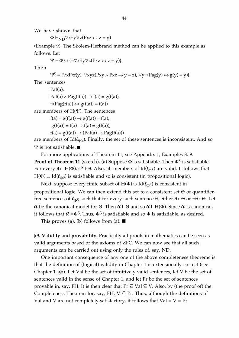
44

We have shown thatΦ©ND∀x∃y∀z(Pxz ↔ z = y)

(Example 9). The Skolem-Herbrand method can be applied to this example asfollows. Let

Ψ = Φ ∪ {¬∀x∃y∀z(Pxz ↔ z = y)}.Then

ΨS = {∀xPxf(y), ∀xyz(Pxy ∧ Pxz → y = z), ∀y¬(Pag(y) ↔ g(y) = y)}.The sentences

Paf(a),Paf(a) ∧ Pag(f(a)) → f(a) = g(f(a)),¬(Pag(f(a)) ↔ g(f(a)) = f(a))

are members of H(Ψ). The sentencesf(a) = g(f(a)) → g(f(a)) = f(a), g(f(a)) = f(a) → f(a) = g(f(a)),f(a) = g(f(a)) → (Paf(a) → Pag(f(a)))

are members of Id(lΨS). Finally, the set of these sentences is inconsistent. And so

Ψ is not satisfiable. �For more applications of Theorem 11, see Appendix 1, Examples 8, 9.

Proof of Theorem 11 (sketch). (a) Suppose Φ is satisfiable. Then ΦS is satisfiable.For every θŒ H(Φ), ϕS[θ. Also, all members of Id(lΦS) are valid. It follows that

H(Φ) ∪ Id(lΦS) is satisfiable and so is consistent (in propositional logic).

Next, suppose every finite subset of H(Φ) ∪ Id(lΦS) is consistent in

propositional logic. We can then extend this set to a consistent set Θ of quantifier-free sentences of lΦS such that for every such sentence θ, either θŒΘ or ¬θŒΘ. Let

A be the canonical model for Θ. Then A[Θ and so A[H(Φ). Since A is canonical,it follows that A[ΦS. Thus, ΦS is satisfiable and so Φ is satisfiable, as desired.

This proves (a). (b) follows from (a). �

§9. Validity and provability. Practically all proofs in mathematics can be seen asvalid arguments based of the axioms of ZFC. We can now see that all sucharguments can be carried out using only the rules of, say, ND.

One important consequence of any one of the above completeness theorems isthat the definition of (logical) validity in Chapter 1 is extensionally correct (seeChapter 1, §6). Let Val be the set of intuitively valid sentences, let V be the set ofsentences valid in the sense of Chapter 1, and let Pr be the set of sentencesprovable in, say, FH. It is then clear that Pr ˘ Val ˘ V. Also, by (the proof of) theCompleteness Theorem for, say, FH, V ˘ Pr. Thus, although the definitions ofVal and V are not completely satisfactory, it follows that Val = V = Pr.

45

Notes for Chapter 2. The Completeness Theorem for FH (Theorem 3 andCorollary 1) with Φ countable is due to Gödel (1930); the problem was formulatedin Hilbert, Ackermann (1928). The generalization to uncountable Φ and thepresent proof are due to Henkin (1949).

The sequent calculus is GS due to Gentzen (1934-35). The active formulas of aninference are usually called “side formulas” of that inference. Lemmas 17 and 19are special cases of a general result due to Kleene (1952a). The InterpolationTheorem (Theorem 4), for a different (complete) logical calculus, is due to Craig(1957a).Theorem 5 is due to Gentzen (1934-35). Gentzen proved that GS iscomplete (Theorem 7) by showing that if ϕ is provable in FH, then ⇒ ϕ isderivable in GS with the Cut Rule and then that all applications of (Cut) can beeliminated from the derivation, Gentzen's Hauptsatz or Cut EliminationTheorem. Direct proofs of essentially Theorem 7, similar to the present proof,were given by Beth (1955), Hintikka (1955), and Kanger (1957). The idea ofthinking of a derivation of a sequent S in GS as the result of an abortive attemptto define a counterexample to S is due to these authors.

Systems of natural deduction were first defined by Jaskowski (1934) andGentzen (1934-35). There are now several such systems (cf. Prawitz (1965)). ND isessentially taken from Mates (1965). ND is closely related to the system of Gentzen(1934-35); more “natural”, perhaps, if only marginally. On the other handGentzen’s system (like GS) lends itself more easily to proof-theoreticalinvestigations (cf. Prawitz (1965)).

Theorem 11, for finite Φ, was first proved by Skolem (1922), (1929) and, with“non-satisfiable” replaced by “refutable in FH”, by Herbrand (1930) (see theintroductions to Skolem (1928) and Herbrand (1930) in van Heijenoort (1967)).

46

3. MODEL THEORY

So far the relation[, as in A[ϕ, has only been used as a tool in defining logicalvalidity and logical consequence and proving the various completenesstheorems. In this chapter we shall study[ for its own sake.

It is one of the basic tasks of model theory (of L1) to investigate the “expressivepower” of L1; in particular, to show that, whereas many important mathematicalconditions (on models) can be expressed in L1 (see Chapter 1, §7), there are natural

conditions that cannot. The most fundamental results of this type are thosepresented in §§1, 2. Also, for example, if a theory T is complete (see §6) and A, Bare models of T, we may conclude that there is no first-order sentence true in Aand false in B.

In this chapter we use© to mean©FH. We also sometimes replace[ by©, and

vice versa, and use “is consistent” and “has a model” interchangably. This isjustified by the Completeness Theorem for FH (Theorem 2.3). We always assumethat the theory referred to by “T” is consistent. For illustrations and applicationsof some of the results proved in this Chapter, see §13.

§1. Basic concepts. In this section we define some of the basic concepts of modeltheory and prove some elementary results.

Th(A), the theory of A, is the set {ϕ: A[ϕ}. Thus, A ≡ B if Th(A) = Th(B). IfA ƒ B, then A ≡ B (Proposition 1.1). Clearly, ≡ is an equivalence relation.

Let K be a class of models. We always assume that all members of K aremodels for the same language lK. Th(K), the theory of K, is the set of sentences ϕsuch that A[ϕ for every AŒK. Mod(ϕ) is the class of models of ϕ. Mod(Φ) is theclass of models of Φ.

A is a submodel of B, and B an extension of A, A ˘ B, if lA = lB, A ˘ B, PA =

PB ∩ An for every n-place predicate PŒlA, fA = fB|A for every n-place functionsymbol fŒlA, and cA = cB for every individual constant cŒlA. (If X is a subset of the

domain of the function g, then g|X = {¤a1,...,an,g(a1,...,an)%: a1,...,anŒX}.)A set X is closed under a function g if g(a1,...,an)ŒX for all a1,...,anŒX. If X ˘ A, A

has a submodel with domain X, written as A|X, iff cAŒX for every individualconstant cŒlA and X is closed under fA for every function symbol fŒlA.

Suppose A = (A,I) and X ˘ A. For every aŒX, let ca be a new constant. Let lA(X)= lA ∪ {ca: aŒX}. Let AX be the expansion of A to lA(X) such that ca

AX = a for aŒX.

A is an elementary submodel of B , and B an elementary extension of A, A ” B ,if A ˘ B and for every formula ϕ and every valuation v: Var → A, A[ϕ[v] iffB[ϕ[v]. Clearly, ” is reflexive, and transitive and if A ” B, then A ˘ B and A ≡ B.Also, A ” B iff A ˘ B and AA ≡ BA.

47

We now prove two basic lemmas on the relation ”.

Lemma 1. Suppose A ˘ B. Then A ” B iff for every formula ∃xϕ of lA and every

v: Var → A, if B[∃xϕ[v], there is an aŒA such that B[ϕ[v(x/a)].

Proof. Suppose first A ” B. Suppose ∃xϕ is a formula of lA such that B[∃xϕ[v].

Then A[∃xϕ[v]. It follows that there is an aŒA such that A[ϕ[v(x/a)]. But thenB[ϕ[v(x/a)], as desired.

We prove the converse implication by induction. Let ψ be a formula of lA and

suppose v: Var → A. We have to show that A[ψ[v] iff B[ψ[v]. Since A ˘ B, thisholds if ψ is atomic. The cases corresponding to the propositional connectives arestraightforward. Suppose ψ := ∃xϕ. If A[∃xϕ[v], there is an aŒA such thatA[ϕ[v(x/a)]. But then, by the inductive assumption, B[ϕ[v(x/a)] and soB[∃xϕ[v]. Next, suppose B[∃xϕ[v]. Then, by assumption, there is an aŒA suchthat B[ϕ[v(x/a)]. By the inductive assumption, A[ϕ[v(x/a)] and so A[∃xϕ[v]. Thecase ψ := ∀xϕ is similar. �

The point of Lemma 1 is that the conclusion A ” B follows from a conditionthat doesn’t mention satisfaction in A.

An automorphism of A is an isomorphism of A onto A.

Corollary 1. Suppose A ˘ B and for any n, any a1,...,anŒA, and any bŒB, there is anautomorphism f of B such that f(ai) = ai for 0 < i ≤ n and f(b)ŒA. Then A ” B.

To simplify the notation in what follows we shall often make no distinctionbetween the members of a model and the corresponding individual constants (orregard the members of A as names of themselves). Thus, if ϕ(x1,...,xn) is a formulaand a1,...,anŒA, we may write ϕ(a1,...,an) for ϕ(ca1,...,can) and A[ϕ(a1,...,an) for

A[ϕ[v], where v(xi) = ai for i ≤ n. But, of course, if B ≠ A, then B[ϕ(a1,...,an) is not

(automatically) defined.Proof of Corollary 1. Suppose ∃yψ(x1,...,xn,y) is a formula of lA and supposea1,...,anŒA are such that B[∃yψ(a1,...,an,y). There is then a bŒB such thatB[ψ(a1,...,an,b). Let f be an automorphism f of B such that f(ai) = ai for 0 < i ≤ nand f(b)ŒA. Then B[ψ(a1,...,an,f(b)). Thus, the condition of Lemma 1 is satisfied

and so A ” B. �The following is a simple illustration of Corollary 1. We want to show that

(Ra, ≤) ” (Re, ≤) (cf. Chapter 1, §7, Example 1). Suppose r1,...,rnŒRa, sŒRe, andr1 ≤...≤ ri < s < ri+1 ≤...≤ rn. Let rŒRa be such that ri < r < ri+1. Now, let f be anyincreasing function on Re onto Re such that f(rj) = rj for j = 1,...,n and f(s) = r. Then

48

f is an automorphism of (Re, ≤) and f(s)ŒRa. And so, by Corollary 1, (Ra, ≤) ”

(Re, ≤), as desired.Let {Ai: iŒI} be a set of models. Suppose {Ai: iŒI} is a chain in the sense that for

all i, jŒI, either Ai ˘ Aj or Aj ˘ Ai. The union of {Ai: iŒI}, ∪{Ai: iŒI}, is then the

model A such that A = ∪{Ai: iŒI}, PA = ∪{PAi: iŒI}, fA = ∪{fAi: iŒI}, and cA = cAi

for every predicate P, function symbol f, and individual constant c. Note that fA isa function. {Ai: iŒI} is an elementary chain if Ai ” Aj or Aj ” Ai for any i, jŒI.

Lemma 2 (Tarski’s Lemma). If {Ai: iŒI} is an elementary chain, then for every jŒI,

Aj ” ∪{Ai: iŒI}.

Proof. Let A = ∪{Ai: iŒI}. We show, by induction, that for every sentence ϕ,

(*) for every jŒI, formula ϕ, and v: Var → Aj, Aj[ϕ[v] iff A[ϕ[v].

This is clear if ϕ is atomic. The inductive steps corresponding to the propositionalconnectives are evident. Let ϕ := ∃xψ. First suppose Aj[ϕ[v]. There is then an aŒAsuch that Aj[ψ[v(x/a)]. But then, by the inductive assumption, A[ψ[v(x/a)] and soA[ϕ[v]. Finally, suppose A[ϕ[v]. Let bŒA be such that A[ψ[v(x/b)]. Since {Ai: iŒI}is a chain, there is kŒI such that Aj ” Ak and bŒAk. By the inductive assumption,Ak[ψ[v(x/b)], whence Ak[ϕ[v] and so Aj[ϕ[v], as desired. The case ϕ := ∀xψ is

similar. �A formula is basic if it is atomic or the negation of an atomic formual. The

(basic) diagram of A, D(A), is then set of basic sentences of lA(A) obtained fromprimitive formulas of lA by replacing free variables by constants ca for aŒA andtrue in AA. The elementary diagram of A, ED(A), is the set of sentences of lA(A)true in AA. The universal diagram of A, UD(A), is the set of universal sentences oflA(A) true in AA. If, as in Lemma 3(d), below, we consider diagrams of two models

A and B at the same time, we assume that the same constants are used in the twodiagrams to correspond to the same objects (common elements of A and B).

f is an embedding of A in B if f(A) ˘ B, A is embeddable in B if there is anembedding of A in B. Thus, A is embeddable in B iff there is a model C ƒ B suchthat A ˘ C. f is an elementary embedding of A in B if f: A → B and for everyformula ϕ and every valuation v: Var → A, A[ϕ[v] iff B[ϕ[f(v)]; in other words,there is an elementary submodel C of B such that f: A ƒ C. A is elementarily

embeddable in B if there is an elementary embedding of A in B.An existential formula ∃x1...xnψ is simple if ψ is a conjunction of primitive

basic formulas. Every existential formula is equivalent to a disjunction of simpleexistential formulas. We write A ”1B to mean that A ˘ B and for every simple

49

existential formula ϕ(x1,...,xn) of lA and all a1,...,anŒA, if B[ϕ(a1,...,an), thenA[ϕ(a1,...,an). (Thus, in fact, A ”1B iff every existential sentence of lA(A) true inBA is true in AA.) A function g is an existential embedding of A in B if g is anembedding of A in B and g(A) ”1B, where g(A) is the image of A under g.

Lemma 3. (a) If B[D(A), then A is embeddable in B.(b) If B[ED(A), then A is elementarily embeddable in B.(c) If B[UD(A), then A is existentially embeddable in B.(d) If A ˘ B and C[ED(A) ∪ D(B), there is an embedding g of B in C such that

g|A is an elementary embedding of A in C.

Here we have taken the liberty of saying, for example, that A is embeddable in Bwhen, strictly speaking, we should have said that A is embeddable in B|lA.

Proof. This is really evident but we nevertheless give a detailed proof of (a); theremaining cases are similar. Suppose B[D(A). Let g: A → B be such that g(a) =caB. Now, suppose, for example PŒlA is a two-place predicate and a, bŒA. If¤a,b%ŒPA, then PcacbŒD(A). It follows that B[Pcacb and so ¤caB,cbB%ŒPB, whence¤g(a),g(b)%ŒPB. Similarly, if ¤a,b%∉PA, then ¤g(a),g(b)%∉PB. Next, suppose fŒlA is,say, a one-place function symbol. Suppose fA(a) = b, where a, bŒA. Then f(ca) =cbŒD(A) and so B[f(ca) = cb, whence fB(caB) = cbB and so fB(g(a)) = g(fA(a)).Finally, let cŒlA be a constant. Let a be such that cA = a. Then c = caŒD(A) and soB[c = ca. But then g(cA) = caB = cB. Thus, g is an embedding of A in B. �

The converse of Lemma 3(a) is also true: If A is embeddable in B, then (someexpansion of) B is a model of D(A); and similarly for Lemma 3(b), (c), (d). Theverification of this is left to the reader.

§2. Compactness and cardinality theorems. In model-theoretic proofs wefrequently want to show that a certain set of sentences has a model. For example,suppose we want to show that a certain set Φ has a model which is an extensionof a given model A. By Lemma 3(a), it is then sufficient (and necessary) to showthat Φ ∪ D(A) has a model. But this may be far from obvious and at the same timeit may be quite clear, or at least (much) easier to prove, that every finite subset ofΦ ∪ D(A) has a model. It is in situations like this, and they occur very often, thatthe following theorem is indispensable.

Theorem 1 (Compactness Theorem). For any set of sentences Φ, if every finitesubset of Φ has a model, then Φ has a model.

50

Proof. This follows at once from the Completeness Theorem for FH (Theorem2.3): Suppose every finite subset of Φ has a model. Then every finite subset of Φ isconsistent. But then Φ is consistent and so Φ has a model. �

Theorem 1 can also be proved directly, without going via a completenesstheorem, by just replacing “Ψ©ψ“ by “there is a finite subset Ψ’ of Ψ such that

“Ψ’[ψ” in the proof of Theorem 2.3. “Ψ is consistent“ then becomes “every finite

subset of Ψ has a model”. In §9 we give a quite different proof of Theorem 1.From the proof of Theorem 1 we obtain the following:

Theorem 2 (Löwenheim-Skolem Theorem). If Φ is a countable set of sentencesand Φ has an infinite model, then Φ has a denumerable model.

For any formula ϕ(x), let ∃>nxϕ(x) :=

∃x0...xn(∧{xi ≠ xj: i < j ≤ n} ∧ ∧{ϕ(xi): i ≤ n}).

LetINF = {∃>nx(x=x): nŒN}.

Proof. The model of Φ ∪ INF constructed in the proof of the Completeness (orCompactness) Theorem is denumerable. �

As a first application of Theorem 1 we have the following:

Proposition 1. If Φ is any set of sentences and Φ has arbitrarily large finite models,then Φ has an infinite model.

Proof. By assumption every finite subset of Φ ∪ INF has a model. It follows thatthe whole set has a model A. A is an infinite model of Φ. �

Let N = (N, +, ., S, 0) be the standard model of arithmetic; S is the successorfunction.

Corollary 2. (Skolem) Th(N) has a denumerable model not isomorphic to N.

Proof. Let c be a new constant and let Φ = Th(N) ∪ {c ≠ 0, c ≠ S(0), c ≠ S(S(0)), ...}.Clearly, every finite subset of Φ has a model. But then, by Theorems 1, 2, Φ has adenumerable model A. Obviously, A f N. �

Our next result is a generalization and strengthening of Theorem 2.

Theorem 3 (Downward Löwenheim-Skolem-Tarski (LST) Theorem). Suppose|lA| ≤ κ, X ˘ A, and |X| ≤ κ ≤ |A|. There is then a model B such that X ˘ B, |B|

= κ, and B ” A.

51

Proof. We define an increasing sequence Y0, Y1, Y2, ... of subsets of A as follows.

Let Y0 ˘ A be such that X ˘ Y0 and |Y0| = κ. Now suppose Yn has been defined

and |Yn| = κ. Let {∃xiϕi: iŒI} be the set of sentences of lA(Yn) of the form indicated

and true in AA. Then |I| = κ. For every iŒI, there is an aiŒA such that

AA[ϕ(xi/ai). Let Yn+1 = Yn ∪ {ai: iŒI}. Then |Yn+1| = κ.

Let Y = ∪{Yn: nŒN}. Then |Y| = κ and Y is closed under the functions fA,

where fŒlA, and cAŒY for every constant cŒlA. Let B = A|Y. Then X ˘ B and |B|= κ. Suppose ∃xϕ is a sentence of l(B) such that AA[∃xϕ. ∃xϕ is a sentence oflA(Yn) for some n. It follows that there is an aŒYn+1 such that AA[ϕ(x/a). Hence,

by Lemma 1, B ” A. �A somewhat different proof of Theorem 3 is as follows. Let A be any Skolem

model and suppose Ø ≠ X ˘ A. The Skolem hull of X in A, HA(X), is then the leastset Y containing X such that cAŒY for all individual constants in lA and Y isclosed under a functions fA such that f is a function symbol in lA. It follows that|X| ≤ |HA(X)| ≤ |X| + |lA| + ℵ0. Let HA(X) = A|HA(X). In what follows we writeH(X), H(X) for HA(X), HA(X), respectively.

Proposition 2. If A is a Skolem model and Ø ≠ X ˘ A, then H(X) ” A.

Proof. Suppose a1,...,anŒH(X) and A[∃yϕ(a1,...,an,y). It follows thatA[ϕ(a1,...,an,fϕ(a1,...,an)). But fϕ(a1,...,an)ŒH(X). Thus, by Lemma 1, H(X) ” A. �

Theorem 3 is an immediate consequence of this and Proposition 1.6.

Theorem 4 (Upward LST Theorem). Suppose |lA| ≤ κ and ℵ0 ≤ |A| ≤ κ. There is

then an elementary extension B of A such that |B| = κ.

Proof. Let {ci: iŒI}, where |I| = κ, be a set of new individual constants. Let Φ =ED(A) ∪ {¬ci = cj: i, jŒI & i ≠ j}. Since A is infinite, every finite subset of Φ has a

model. By the Compactness Theorem, it follows that Φ has a model C. By Lemma3(b), we may assume that A ” C|lA. Clearly, |C| ≥ κ. By Theorem 3, there is amodel B such that A ˘ B, B ” C|lA, and |B| = κ. But then A ” B and so B is as

desired. (This application of Theorem 3 is not really necessary, since the model ofΦ defined in the proof of the Compactness Theorem is of cardinality κ.) �

Corollary 3 (LST or Cardinality Theorem). Let Φ be any set of sentences andsuppose κ ≥|Φ|. If Φ has an infinite model, then Φ has a model of cardinality κ.

52

§3. Elementary and projective classes. A class K is elementary, KŒEC, if there is asentence ϕ such that K = Mod(ϕ). K is ∆-elementary, KŒEC∆, if there is a set Φ ofsentences such that K = Mod(Φ). Kc = {A: lA = lK & A∉K}.

Proposition 3. If K = Mod(Φ) and KŒEC, there is a finite subset Ψ of Φ such that K= Mod(Ψ).

Proof. Let ϕ be such that K = Mod(ϕ). Then Φ ∪ {¬ϕ} has no model. But then thereis a finite subset Ψ of Φ such that Ψ ∪ {¬ϕ} has no model. It follows that Mod(Φ) ˘

Mod(Ψ) and Mod(Ψ) ∩ Mod(¬ϕ) = Ø and so K = Mod(Ψ). �From Propositions 1, 3 we obtain the following:

Corollary 4. Suppose KŒEC∆ and K has arbitrarily large finite members. Then

(i) K has an infinite member,(ii) the class of infinite members of K is EC∆ but not EC.

Proof. (i) This is Proposition 1.(ii) If Mod(Φ ∪ INF) is EC, by Proposition 3, there is a member ϕ of INF such

that K = Mod(Φ ∪ ϕ), which is not true. �By Corollary 4, the classes of finite linear orderings, finite Boolean algebras,

finite groups etc. are not EC∆ and the classes of infinite linear orderings, Booleanalgebras, groups etc., although EC∆, are not EC.

That there are classes KŒEC∆ – EC can also be shown without using theCompactness Theorem. If we allow lK to be infinite, this is clear.

A slightly less trivial example is this. Let P be a one-place predicate and let K beany EC∆ class of infinite models for {P}. Every sentence of {P} which has a model

has a finite model (see, §13, Example 1). It follows that K∉EC.Yet another way of showing that EC∆ ≠ EC, for a quite different but still rather

trivial reason, is this. Suppose l is finite and contains a two-place predicate (or aone-place function symbol). Then there are 2ℵ0 EC∆ classes of models for l butonly ℵ0 EC classes of such models.

K is closed under isomorphisms if for all A, B, if AŒK and B ƒ A, then BŒK. Kis closed under ≡ if for all A, B, if AŒK and B ≡ A, then BŒK. By Proposition 1.1, ifK is closed under ≡, then K is closed under isomorphisms. Clearly, if KŒEC∆,

then K is closed under ≡.There are classes K∉EC∆ that are closed under ≡. By Corollary 4, one example

is the class of finite models for a given language. But this, too, is true forcardinality reasons. If l is countable and contains a two-place predicate, there are

53

22ℵ0 classes of models for l closed under ≡ but only 2ℵ0 such EC∆ classes.

Proposition 4. (a) If K0, K1ŒEC∆ and K0 ∩ K1 = Ø, there is a class KŒEC such thatK0 ˘ K and K ∩ K1 = Ø.

(b) KŒEC iff KŒEC∆ and KcŒEC∆.

Proof. (a) Let Φi be such that Ki = Mod(Φi), i = 0, 1. Then Φ0 ∪ Φ1 has no model. Itfollows that there is a finite subset Ψ of Φ0 such that Ψ ∪ Φ1 has no model. Let K =

Mod(∧Ψ).

(b) “⇒” is clear. “⇐” follows from (a). �K is a projective (or pseudo-elementary) class, KŒPC, if there is a K’ŒEC such

that K = {A|lK: AŒK’}. In other words, there is a sentence ϕ of lK’ such that K is

the class of models of the second-order sentence obtained from ϕ by existentiallyquantifying the members of lK’ – l. KŒPC∆ if there is a K’ŒEC∆ such that K =

{A|lK: AŒK’}. Clearly, EC ˘ PC and EC∆ ˘ PC∆.

From Corollary 4 it follows that:

Corollary 5. If KŒPC∆ and K has arbitrarily large finite members, then K has aninfinite member. In particular, the class of finite models for a given language innot PC∆.

On the other hand, the class of infinite members of an EC∆ (PC, PC∆) class is stillEC∆ (PC, PC∆).

PC classes need not be closed under ≡. One example is as follows. Let < and Pbe a two-place and a one-place predicate, respectively. Let ϕ be a sentence sayingthat “< is a linear ordering and P is nonempty and has no <-smallest element”.Let K = Mod(ϕ)|{<}. Then KŒPC and (A, <)ŒK iff (A, <) is a linear ordering whichis not a well-ordering. Now let (A’, <’) be any infinite well-ordering. (A’, <’)œK.

Let cn, nŒN, be individual constants. Let Φ = Th((A’, <’)) ∪ {ck < cm: m < k}. Every

finite subset of Φ has a model and so Φ has a model (A’’, <’’, an)nŒN. (A’’, <’’) ≡(A’, <’) and (A’’, <’’)ŒK. Thus, K is not closed under ≡. It follows that PC h EC∆.

Proposition 4 can be strengthened as follows.

Proposition 5. If K0, K1ŒPC∆ and K0 ∩ K1 = Ø, there is a class KŒEC such that K0˘ K and K ∩ K1 = Ø. Thus, in particular, if K and Kc are PC∆, then K is EC.

Proof. Let Φi be such that Ki = {A|l: A[Φi}, i = 0, 1. We may assume that lΦ0 ∩ lΦ1

= l. Since K0 ∩ K1 = Ø, there are finite subsets Ψ0 and Ψ1 of Φ0 and Φ1,

54

respectively, such that Ψ0 ∪ Ψ1 has no model. Let ψi := ∧Ψi. Then[ψ0 → ¬ψ1. By

the Interpolation Theorem (Theorem 2.8; cf. also Theorem 8, below), there is asentence θ of l such that[ψ0 → θ and[θ → ¬ψ1. Let K = Mod(θ). �

The relation between PC∆ and EC∆ is given in the following:

Proposition 6. KŒEC∆ iff KŒPC∆ and K is closed under ≡.

Proof. “⇒” is clear. “⇐”. Let Φ = Th(K). It is sufficient to show that K = Mod(Φ).Clearly, K ˘ Mod(Φ). To show that Mod(Φ) ˘ K, suppose A[Φ. Every finite subsetof Th(A) has a model in K. Indeed, suppose there is a sentence ϕ such that A[ϕand ϕ has no model in K. Then ¬ϕŒΦ and so A[¬ϕ, a contradiction. Let Ψ besuch that K = Mod(Ψ)|lK. Then every finite subset of Th(A) ∪ Ψ has a model. LetB be a model of Th(A) ∪ Ψ and let C = B|lK. Then CŒK and A ≡ C. It follows that

AŒK, as desired. �

§4. Preservation theorems. One important aspect of model theory is the study ofthe relation between syntactic properties of (sets of) sentences and algebraicproperties of the corresponding classes of models. So-called preservationtheorems are particularly clear examples of results of this type.

A class K of models is closed under submodels if for all A, B, if AŒK and B ˘ A,then BŒK. Let ϕ be a universal sentence, ϕ := ∀x1...xnψ(x1,...,xn), where ψ(x1,...,xn) isquantifier-free. Suppose A[ϕ and B ˘ A. Let b1,...,bn be any members of B. ThenA[ψ(b1,...,bn). Since ψ(x1,...,xn) is quantifier-free, we have B[ψ(b1,...,bn). It follows

that B[ϕ. Thus, ϕ is preserved under submodels in the sense that Mod(ϕ) isclosed under submodels. A theory is universal if all its members (axioms) areuniversal. It follows that a universal theory T is preserved under submodels inthe sense that Mod(T) is closed under submodels.

We now show that the converse of this is also true and so we have thefollowing:

Theorem 5 (Łos -Tarski Theorem). Τ is preserved under submodels iff T isequivalent to a universal theory.

Proof. “⇒”. Let T’ be the set of universal sentences ϕ such that Τ©ϕ. Then Mod(T)˘ Mod(T’). To show that Mod(T’) ˘ Mod(T), suppose A[T’. We want to show

that T ∪ D(A) has a model. Suppose not. There is then a conjunction ψ(c1,...,cn) ofmembers of D(A), where ψ(x1,...,xn) is a formula of lT, such that T©¬ψ(c1,...,cn). Letθ := ∀x1...xn¬ψ(x1,...,xn). Then T© θ, whence θŒT’ and so A[θ. On the other

55

hand, since ψ(c1,...,cn) is a conjunction of members of D(A), it is clear that A[¬θ, a

contradiction. It now follows that T ∪ D(A) has a model B. By Lemma 3(a), A isembeddable in B. But then, since T is preserved under submodels, A[T, asdesired. �

The conjunction of two universal sentences is equivalent to a universalsentence. Thus, combining Theorem 5 and Proposition 3 we get:

Corollary 6. For any sentence ϕ, ϕ is preserved under submodels iff ϕ is equivalentto a universal sentence.

A simple illustration of Corollary 6 is as follows. Let ϕ :=∃xy∀z(f(z) = x ∨ f(z) = y).

Clearly, ϕ is preserved under submodels. Thus, there is a universal sentenceequivalent to ϕ. And, of course, ϕ is equivalent to

∀xyz(f(x) = f(y) ∨ f(x) = f(z) ∨ f(y) = f(z)).A formula is universal-existential or ∀∃ if it is of the form

(*) ∀x1...xnψ(x1,...,xn),where ψ(x1,...,xn) is existential. (Universal and existential formulas are ∀∃.) A set

of sentences is ∀∃ if all its members are.A class K is closed under unions of chains if for any chain {Ai: iŒI} ˘ K,

∪ {Ai: iŒI}ŒK. T is preserved under unions of chains if Mod(T) is closed under

unions of chains. Note that if T is preserved under submodels, then T ispreserved under unions of chains.

Suppose {Ai: iŒI} is a chain of models of (*). Let A = ∪{Ai: iŒI}. To see that A is

then a model of (*), let a1,...,an be any members of A. Since {Ai: iŒI} is a chain,there is an Ai such that a1,...,anŒAi. Since Ai is a model of (*), we haveAi[ψ(a1,...,an) and so, since ψ(x1,...,xn) is existential and Ai ˘ A, A[ψ(a1,...,an).

Thus, A is a model of (*). It follows that any ∀∃ theory is preserved under unionsof chains.

We now show that the converse of this is also true and so we have thefollowing:

Theorem 6 (Chang-Łos -Suszko Theorem). T is preserved under unions of chainsiff T is equivalent to an ∀∃ theory.

Lemma 4. Let T’ be the set of ∀∃ sentences ϕ such that T©ϕ. Suppose A[T’. There

is then a model B such that B[T and A ”1B.

56

Proof. By Lemma 3(c), it is sufficient to show that T ∪ UD(A) has a model.Suppose not. There are then a universal formula ψ(x1,...,xn) and constants c1,...,cn

not occurring in T such that AA[ψ(c1,...,cn) and T©¬ψ(c1,...,cn). Let ϕ :=∀x1...xn¬ψ(x1,...,xn). Then ϕ is (equivalent to) an ∀∃ sentence, T©ϕ, and A]ϕ,

contrary to assumption. �

Lemma 5. Suppose A ”1B. Then there is a model C such that A ” C and B ˘ C.

Proof. By Lemma 3(d), it is sufficient to show that ED(A) ∪ D(B) has a model.Suppose not. There is then a conjunction ϕ(a1,...,ak,b1,...,bn) of members of D(B),where ϕ(x1,...,xk,y1,...,yn) is a formula of lA, a1,...,ak∈A, b1,...,bn∈B – A such thatED(A)©¬∃y1...ynϕ(a1,...,ak,y1,...,yn). Let ψ(x1,...,xk) := ∃y1...ynϕ(x1,...,xk,y1,...,yn). Itfollows that A[¬ψ(a1,...,ak). On the other hand ψ(x1,...,xk) is simple andB[ψ(a1,...,ak) and so, since A ”1B, A[ψ(a1,...,ak), a contradiction. �Proof of Theorem 6. “⇒”. Let T’ be as in Lemma 4. Then Mod(T) ˘ Mod(T’). To

show that Mod(T’) ˘ Mod(T), suppose A[T’. We are going to show that there is a

model B of T such that A ” B. From this it follows that A[T. We construct asequence A0, A1, A2, ... of models such that A0 = A and for all n,(1) A2n[T’,(2) A2n+1[T,(3) An ˘ An+1,(4) A2n ” A2n+2.Suppose A2n has been defined and (1) holds; this is true for n = 0. Then, by Lemma4, there is a model A2n+1 such that (2) holds and A2n ”1A2n+1. Finally, by Lemma 5,this implies that there is a model A2n+2 such that (4) holds, whence A2n+2[T’, and

A2n+1 ˘ A2n+2.

Now, let

B = ∪{An: nŒN}.

Then, by (3),

B = ∪{A2n: nŒN} = ∪{A2n+1: nŒN}.

By (4) and Lemma 2, A ” B. By (2) and the fact that T is preserved under unions ofchains, B[T. It follows that A[T, as desired. �

Corollary 7. A sentence is preserved under unions of chains iff it is equivalent toan ∀∃ sentence.

A simple illustration of Corollary 7 is as follows. Let ϕ :=∀x∃y∀z(Pxz ↔ z = y).

57

ϕ says that “the relation P is a function”. The union of a chain of functions is afunction. Thus, ϕ is preserved under unions of chains. And, of course, ϕ isequivalent to the conjunction of

∀x∃yPxy and∀xyz(Pxy ∧ Pxz → y = z)

and this conjunction is equivalent to an ∀∃ sentence.Suppose A and B are models for l. A function h is a homomorphism of A onto

B if h is a function on A onto B such that for all a1,...,anŒA,if ¤a1,...,an%ŒPA, then ¤h(a1),...,h(an)%ŒPB,

h(cA) = cB,h(fA(a1,...,an)) = fB(h(a1),...,h(an)),

for predicates P, constants c, and function symbols f of l.B is a homomorphic image of A if there is a homomorphism of A onto B.

Note that homomorphic images of the same model need not be isomorphic, noteven if the homomorphisms in question are the same.

A formula ϕ is positive if the only logical symbols occurring in ϕ are ∧, ∨, ∀, ∃,=. T is positive if all its axioms are positive. We write AΣ+B to mean that everypositive sentence true in A is true in B.

The proof of the following lemma is straightforward (compare the proof ofProposition 1.1).

Lemma 6. Suppose h is a homomorphism on A onto B and all v : Var → A. Thenfor every term t of l,

h(tA[v]) = tB[hv].Also, for every positive formula ϕ of l,

if A[ϕ[v], then B[ϕ[hv].In particular, if B is a homomorphic image of A, then AΣ+B.

K is closed under homomorphisms if for all A, B , if AŒK and B is ahomomorphic image of A, then BŒK. A sentence ϕ (theory T) is preserved under

homomorphisms if Mod(ϕ) (Mod(T)) is closed under homomorphisms. ByLemma 6, positive sentences and, therefore, positive theories are preservedunder homomorphisms.

The converse of this is also true and so we have the following:

Theorem 7 (Lyndon). Τ is preserved under homomorphisms iff T is equivalent toa positive theory.

58

Lemma 7. If A0Σ+A1, there are models B0, B1 such that Bi ≡ Ai, i = 0, 1, and B1 is ahomomorphic image of B0.

This can be proved in a number of different ways. Our proof, in Appendix 2, usesa variant of some ideas that will be presented in §7 and in Chapter 5.Proof of Theorem 7. “⇒”. Suppose T is preserved under homomorphisms. Let T’be the set of positive sentences ϕ such that T[ϕ. Then Mod(T) ˘ Mod(T’). To

prove that Mod(T’) ˘ Mod(T), suppose A[T’. Let

Φ = T ∪ {¬ϕ: ϕ positive and A[¬ϕ}.Φ has a model. For, suppose not. There are then positive sentences ϕ0,...,ϕn suchthat A[¬ϕk, for k ≤ n, and T[ϕ0 ∨...∨ ϕn and so A[ϕ0 ∨...∨ ϕn, which is a

contradiction.Let B be a model of Φ. Then B[T and BΣ+A. By Lemma 7, there are A’, B’

such that A’ ≡ A, B’ ≡ B, and A’ is a homomorphic image of B’. Thus, B’[T andso A’[T and so A[T, as desired. �

Corollary 8. A sentence is preserved under homomorphisms iff it is equivalent toa positive sentence.

The preservation theorems prove in this section are exemplified by some of thetheories defined in Chapter 1, §7. Thus, for example, (i) the classes of linearorderings, Boolean algebras, and (Abelian) groups are closed under submodelsand the corresponding theories are universal; (ii) the classes of fields, algebraicallyclosed fields, ordered fields, and real closed ordered fields are closed under unionsof chains and the corresponding theories are ∀∃; (iii) the classes of groups andAbelian groups and, if we omit the axiom 0 ≠ 1, Boolean algebras are closed underhomomorphisms and the corresponding theories are positive.

§5. Interpolation and definability. In Chapter 2, §4 we outlined a proof of thefollowing result (Theorem 2.8).

Theorem 8 (Craig’s Interpolation Theorem). Let ϕ, ψ be any two sentences. If[ϕ → ψ, there is sentence θ of lϕ ∩ lψ such that[ϕ → θ and[θ → ψ.

We shall now give a purely model-theoretic proof of this. We derive Theorem 8from the following result.

A set Φ is complete if for every sentence ϕ of lΦ, either Φ[ϕ or Φ[¬ϕ.

59

Theorem 9 (Robinson’s Consistency Theorem). Let l = l0 ∩ l1 and let Φ be acomplete consistent set of sentences of l. Let Φi be a consistent set of sentences ofli such that Φ ˘ Φi, i = 0, 1. Then Φ0 ∪ Φ1 is consistent.

Lemma 8. Suppose Ai is a model for li, i = 0, 1, and let l = l0 ∩ l1.

(a) If B is a model for l1 and A0|l ≡ B|l, there is a model C for l1 such that A0|l ”

C|l and C ≡ B.(b) If A0|l ” A1|l, there is a model B for l0 such that A0 ” B and A1|l ” B|l.

Proof. (a) By Lemma 3, it suffices to show that the set ED(A0|l) ∪ Th(B) has amodel. Suppose not. There are then a formula ϕ(x1,...,xn) of l and constants c1,...,cn

not in l1 such that ϕ(c1,...,cn)ŒED(A0|l) and Th(B)[¬ϕ(c1,...,cn). It follows that

Th(B) ∪ {∃x1...xkϕ} has no model. But this is not true, since the fact that A0|l ≡ B|l

implies that B is a model of this set.(b) By Lemma 3, it suffices to show that the set ED(A0) ∪ ED(A1|l) has a model.

Suppose not. There are then a formula ϕ(x1,...,xn) of l(A1) and constants c1,...,cn notin l0(A0) such that ϕ(c1,...,cn)ŒED(A1|l) and ED(A0)[¬ϕ(c1,...,cn). It follows thatED(A0) ∪ {∃x1...xkϕ} has no model. But this is not true, since the fact that A0|l ”

A1|l implies that A0A0 is a model of this set. �

Proof of Theorem 9. Let A0 be any model of Φ0. There is a model B of Φ1. A0|l and

B|l are models of Φ and so A0|l ≡ B|l. By Lemma 8(a), it follows that there is a

model A0|l ” A1|l and A1 ≡ B. It follows that A1[Φ1. Starting from A0, A1 andapplying Lemma 8(b) we can now define models An for n ≥ 2 such that for all n,(1) A2n[Φ0,(2) A2n+1[Φ1,(3) An ” An+2,(4) An|l ” An+1|l.

Now let

C0 = ∪{A2n: nŒN} and C1 = ∪{A2n+1: nŒN}.

Then, by (1), (2), (3), and Lemma 2, Ci[Φi, i = 0, 1. Also, clearly, C0|l = C1|l. Itfollows that C0 and C1 have a common expansion C to l0 ∪ l1. C[Φ0 ∪ Φ1. �

There is an alternative proof of Theorem 9 in Appendix 2.Proof of Theorem 8. Let

Θ = {θ: θ sentence of lϕ ∩ lψ and[ϕ → θ}.We are going to show that Θ ∪ {¬ψ} has no model. Suppose it does and let A besuch a model. Then Th(A) ∪ {¬ψ} is consistent. Also Th(A) ∪ {ϕ} has a model. Forsuppose not. Then there is a sentence χŒTh(A) such that[ϕ → ¬χ. But then¬χŒΘ and so A[¬χ, a contradiction. Thus, Th(A) ∪ {ϕ} has a model. Applying

60

Theorem 9 we may now conclude that {ϕ, ¬ψ} (in fact, Th(A) ∪ {ϕ, ¬ψ}) isconsistent. But then]ϕ → ψ, contrary to hypothesis.

This shows that Θ ∪ {¬ψ} has no model. Since Θ is closed under conjunction,it follows that there is a θŒΘ such that[θ → ψ. But also[ϕ → θ and θ is asentence of l. Thus, θ is as desired. �

We have derived Theorem 8 from Theorem 9. It is worth noting that we canalso derive Theorem 9 from Theorem 8: Assume Theorem 8 and let Φ, l, Φi, li, i =0, 1, be as assumed in Theorem 9. Suppose Φ0 ∪ Φ1 has no model. There are thenconjunctions ϕ0, ϕ1 of members of Φ0 and Φ1, respectively, such that[ϕ0 → ¬ϕ1.But then, by Theorem 8, there is a sentence ψ of l such that[ϕ0 → ϕ and[ϕ →¬ϕ1. It follows that Φ0[ϕ and Φ1[¬ϕ, whence Φ[ϕ and Φ[¬ϕ, contrary to

assumption.We shall now use Theorem 8 to prove a basic result on definability. We shall

only discuss definability of predicates but our discussion can easily be extended tofunction symbols and individual constants.

A predicate F is implicitly defined in T if for any two models A and B of T, ifA|(lT–{F}) = B|(lT–{F}), then FA = FB. F is explicitly definable in T if there is aformula ϕ(x1,...,xn) of lT–{F} such that(*) T©∀x1...xn(Fx1...xn ↔ ϕ(x1,...,xn)).

Note that, by compactness, if F is implicitly defined in T, then there is a finitesubtheory T’ of T such that F is implicitly defined in T’.

Suppose (*) is true. Let T’’ be obtained from T by replacing Fx1...xn everywhere

by ϕ(x1,...,xn). (We assume that no variable occurring in T is bound in ϕ(x1,...,xn).)Then T’’ plus (*) is equivalent to T.

Clearly, explicit definability implies implicit definability. Thus, to show that Fis not explicitly definable in T it is sufficient to show that it is not implicitlydefined in T. This is known as Padoa’s method. (Of course, nowadays this is justcommon sense.) The question arises if Padoa’s method is complete in the sensethat the converse of this holds so that if F is not explicitly definable, this can atleast in principle be shown by applying Padoa’s method. In view of the followingresult the answer is affirmative.

Theorem 10 (Beth’s Definability Theorem). Suppose F is an n-place predicateimplicitly defined in T. Then F is explicitly definable in T.

Proof. Let F’ be an n-place predicate not in lT. For every formula ψ of lT, let ψ’ be

obtained from ψ by replacing F by F’. Let T’ = {ψ’: ψŒT}. Let c1,...,cn be new

individual constants. Since F is implicitly defined in T, it follows that

61

T ∪ T’©Fc1...cn → F’c1...cn.

But then there is a sentence ψ of lT such that T©ψ and©ψ ∧ Fc1...cn → (ψ’ → F’c1...cn).

By Theorem 8, there is then a formula ϕ(x1,...,xn) of lT–{F} such that©ψ ∧ Fc1...cn → ϕ(c1,...,cn),©ϕ(c1,...,cn) → (ψ’ → F’c1...cn).

From the latter of these and since F’ does not occur in ϕ(x1,...,xn), it follows that

©ψ → (ϕ(c1,...,cn) → Fc1...cn).

Thus we get©ψ → (Fc1...cn ↔ ϕ(c1,...,cn))

and so, since T©ψ and c1,...,cn do not occur in T, (*) holds, as desired. �

A result similar to Theorem 10 but dealing with a different notion of (explicit)definability is proved in Appendix 3.

§6. Completeness and model completeness. Let A be any model. Suppose that wewant to know what is true and what is not about A (restricted to first-ordersentences). We may approach this problem by writing down a number ofsentences that (we know) are true of A; call these the axioms of our (tentative)theory T of A. We will then want to know if these axioms are sufficient, in otherwords, if A[ϕ implies that T©ϕ. It does iff the theory T is complete in the sensethat for every sentence ϕ of lT, either T©ϕ or T©¬ϕ. There are several ways of

proving that (first-order) theories are complete; two of these will be presented inthis section, a third method in the next.

A result to the effect that a given theory T is complete can also be regarded as a(negative) result on the expressive power of L1: if A, B are any models of T, there

is no sentence ϕ such that ϕ is true in A but not in B.The proof of the following lemma is straightforward.

Lemma 9. The following conditions are equivalent.(i) T is complete.(ii) Any two models of T are elementarily equivalent.(iii) T = Th(A) for some model A.

Clearly, isomorphic models are of the same cardinality. Thus, by Corollary 3, notheory which has an infinite model is categorical in the sense that all its modelsare isomorphic. But there is an interesting weaker notion: a theory T is κ-categorical (or categorical in κ) if T has a model of cardinality κ and all models ofT of cardinality κ are isomorphic.

62

Theorem 11 (Łos -Vaught Test). If all models of T are infinite and T is κ-categorical for some κ ≥ |T|, then T is complete.

Proof. Suppose T is not complete. Let ϕ be a sentence such that T£ϕ and T£¬ϕ.Then T ∪ {¬ϕ} and T ∪ {ϕ} are consistent. By Corollary 3, T ∪ {¬ϕ} has a model Aof cardinality κ. Similarly, T ∪ {ϕ} has a model B of cardinality κ. Clearly, A f Band so T is not κ-categorical. �

By a classical theorem of Steinitz, ACF(p), the theory of algebraically closedfields of characteristic p, where p is 0 or a prime, is κ-categorical for every κ > ℵ0.

Since ACF(p) has no finite models, by Theorem 11, it follows that:

Theorem 12. ACF(p), where p is 0 or a prime, is complete.

For further applications of Theorem 11, see §13, Examples 2, 4, 6, 7.But, of course, there are (important) complete theories that are not κ-

categorical for any κ. To deal with some of these we introduce the concept ofmodel completeness, which is also of independent interest.

A theory T is model-complete if for any two models A, B of T, if A ˘ B, thenA ” B. A is an existentially closed model for T if A[T and for every model B of T,if A ˘ B, then A ”1B.

Theorem 13 (Robinson’s Test). T is model-complete iff every model of T isexistentially closed for T.

Proof. “⇒” is clear. To prove “⇐” suppose A, A’ are models of T and A ˘ A’. Weshow that there are models An of T, n = 0, 1, 2, ..., such that A0 = A, A1 = A’ and for

all n,(1) An ˘ An+1,(2) An ” An+2.Suppose An and An+1 have been defined. Since they are models of T, (1) holds, andAn is existentially closed for T, it follows that An ”1An+1. But then, by Lemma 5,there is a model An+2 such that An ” An+2 and An+1 ˘ An+2. Thus, An+2 is as desired.

Now let

B = ∪{A2n: nŒN} = ∪{A2n+1: nŒN}.

Then, by (2) and Lemma 2, A ” B and A’ ” B. It follows that A ” A’, as desired. �

For some simple direct applications of Robinson’s test, see §13, Examples 2, 4.A theory T was originally defined to be model-complete if T ∪ D(A) is

63

complete for every model A of T. The two definitions are easily equivalent.One of the most important applications of Theorem 13 is the proof of the

following theorem; RCOF, the theory of real closed ordered fields, is not κ-categorical for any κ.

Theorem 14. RCOF is model-complete.

This is proved, modulo an algebraic lemma, in Appendix 4.A model-complete theory need not be complete (see Theorem 18, below, and

§13, Example 2). But we do have the following result. A is a prime model of atheory T if A[T and A is embeddable in every model of T.

Theorem 15. If T is model-complete and has a prime model, then T is complete.

Proof. Let A, B be any models of T. By Lemma 9, it is sufficient to show that A ≡ B.By hypothesis, there is a model C of T which is embeddable in A and B. Since T ismodel-complete, this implies that C ≡ A and C ≡ B and so A ≡ B. �

RCOF has a prime model, the ordered field of real algebraic numbers. Thus,from Theorems 14 and 15 it follows that:

Theorem 16 (Tarski’s Theorem). RCOF is complete.

Combining Lemma 2 and Theorem 6 we get:

Corollary 9. If T is model-complete, then T is equivalent to an ∀∃ theory.

Given Corollary 9 the question arises if every complete ∀∃ theory is model-complete. This, however, is not true (see §13, Example 8) but we do have thefollowing:

Theorem 17. Suppose T is ∀∃, all models of T are infinite, and T is κ-categoricalfor some κ ≥ |T|. Then T is model-complete.

Lemma 10. Suppose κ ≥ |T| and all models of T are infinite. If every model of Tof cardinality κ is existentially closed for T, then T is model-complete.

Proof. Suppose T is not model-complete. By Theorem 13, there are then infinitemodels A, B of T such that A ˘ B and A m1B. By the LST theorem (Corollary 3),

there is a model (C,D) ≡ (B,A) such that |D| = κ. C|D is a model of T of cardinality

64

κ which is not existentially closed for T. �

Lemma 11. Suppose T is preserved under unions of chains and κ ≥ |T|.Then forevery model A of T such that |A| = κ, there is an existentially closed model A* forT such that A ˘ A* and |A*| = κ.

Proof. We first show that(*) for every model B of T such that |B| = κ, there is a model B’ of T such that

B ˘ B’, |B’| = κ, and for every existential sentence of lT(B) and every

model C of T such that B’ ˘ C, if C[ϕ, then B’[ϕ.

Let {ϕξ: ξ < κ} be the set of existential sentences of lT(B). We define models Bξ of Tof cardinality κ for ξ < κ as follows. B0 = B. Suppose Bξ has been defined. If thereis a model C of T extending Bξ such that C[ϕξ, let Bξ+1 be such a model ofcardinality κ. Otherwise, let Bξ+1 = Bξ. If ξ < κ is a limit ordinal, let Bξ =

∪{Bη: η < ξ}. Then Bξ[T.

Now let B’ = ∪{Bξ: ξ < κ}. Then B’[T. Let ϕ be any existential sentence of

lT(B) and suppose there is a model C of T such that B’ ˘ C and C[ϕ. ϕ := ϕξ for

some ξ < κ. Bξ ˘ C. It follows that Bξ+1[ϕξ and so B’[ϕξ. Thus, B’ is as claimed

in (*).We now define An such that An[T, for nŒN, as follows. Let A0 = A. Suppose An

has been defined. Let An+1 be a model related to An the way B’ is related to B in (*).

Finally, let

A* = ∪{An: nŒN}.

Then A*[T. Now let ϕ be any existential sentence of lT(A*) and suppose there is amodel B of T such that A* ˘ B and B[ϕ. ϕ is a sentence of lT(An) for some n. An ˘

B. It follows that An+1[ϕ and so A*[ϕ. Thus, A* is as desired. �

Theorem 17 now follows from Lemmas 10, 11. �ACF(p) is ∀∃ and κ-categorical for every κ > ℵ0 and has no finite models. It

follows, by Theorem 17, that ACF(p) is model-complete. Moreover, any extensionof a field of characteristic p is of characteristic p. Thus, we have the following:

Theorem 18. ACF is model-complete.

The fact that a theory T is model-complete is sometimes interesting not onlybecause it may be used to prove that T is complete. One reason is the following:

65

Theorem 19. If T is model-complete iff for every formula ϕ(x1,...,xn), there is anexistential formula χ(x1,...,xn) such that

T©ϕ(x1,...,xn) ↔ χ(x1,...,xn).

This follows from our next lemma (compare Corollary 6).

Lemma 12. Let ϕ(x1,...,xn) be any formula of lT. Suppose for any models A, B of Tand any a1,...,an∈A, if A ˘ B and A[ϕ(a1,...,an), then B[ϕ(a1,...,an). There is thenan existential formula ψ(x1,...,xn) such that

T©ϕ(x1,...,xn) ↔ ψ(x1,...,xn).

In what follows we sometimes write x , y , ... for finite sequences x1,...,xk, y1,...,ym, ...of variables, c , d , ... for finite sequences c1,...,ck, d1,...,dm, ... of constants, and a , b , ...for finite sequences a1,...,ak, b1,...,bm, ... of elements of models. The length of these

sequences will, in case it matters, be determined by the context. Thus, forexample, ∃ y ϕ( c , y ) is (or may be) short for ∃y1...ynϕ(c1,...,ck,y1,...,yn).

Proof of Lemma 12. LetΦ = {χ( x ): χ is existential & T©χ( x ) → ϕ( x )}.

Let c1,...,cn be new individual constants and let

Ψ = T ∪ {ϕ( c )} ∪ {¬χ( c ): χŒΦ}.If Ψ has no model, we are done. Thus, suppose it does and let (A, a )[Ψ. Then

Θ = T ∪ {¬ϕ( c )} ∪ D((A, a ))has a model. Indeed, if not, there are d1,...,dmœlT ∪ {c1,...,cn} and a quantifier-freeformula ψ( x , y ) of lT such that χ( c , d ) is a conjunction of members of D((A, a )) and

T©χ( c , d ) → ϕ( c ) and soT© ∃ y χ( x , y ) → ϕ( x ).

It follows that ∃ y χ( x , y )ŒΦ and so(A, a )[¬∃ y χ( c , y ).

But also (A, a )[∃ y χ( c , y ), which is a contradiction.Thus, given that (A, a )[Ψ, Θ has a model, which we may assume to be of the

form (B, a ), where A ˘ B. But then ϕ( c ) is true in (A, a ) but not in (B, a ), contraryto assumption. It follows that Ψ has no model and so the proof is complete. �Proof of Theorem 19. “⇐”. Suppose A, B are models of T and A ˘ B. Let ϕ( x ) beany formula and let a1,...,anŒA be such that A[ϕ( a ). Let χ( x ) be an existential

formula such that T©ϕ ↔ χ. Then A[χ( a ). Since χ is existential, it follows thatB[χ( a ) and so that B[ϕ( a ). This shows that A ” B, as desired.

“⇒”. This follows from Lemma 12. �By Theorem 19, given that T is model-complete, we know a great deal about

66

what sets and relations are definable in models of T. Thus, even if, as in the caseof ACF(p), we already know that T is complete it may still be of interest to showthat T is model-complete.

In view of Theorems, 14, 19, every formula of RCOF is equivalent in RCOF toan existential formula. In fact, this can be improved: RCOF admits quantifierelimination, i.e., every formula of RCOF is equivalent to a quantifier-freeformula. Similarly, ACF admits quantifier elimination.

We conclude this § by showing that a model-complete theory T is uniquelydetermined by the set of universal sentences provable in T.

Let us say that T and T’ are u-equivalent if they prove the same universal

sentences.

Theorem 20. If T and T’ are model-complete and u-equivalent, then T and T’ are

equivalent.

The proof of the following Lemma is almost the same as that of Theorem 5.

Lemma 13. Suppose lT = lT’ and for every universal sentence ϕ, if T©ϕ, then

T’©ϕ. Then for every A[T’, there is a B[T such that A ˘ B.

Proof of Theorem 20. By symmetry, it is sufficient to show that every model of Tis a model of T’. Suppose A[T. Then, by Lemma 13, there are models A0 ˘ A1 ˘

A2 ˘ ... such that A0 = A, A2n[T, and A2n+1[T’. Let

B = ∪{A2n: nŒN} = ∪{A2n+1: nŒN}.

Then, since T and T’ are model-complete, A0 ” B[T’ and so A[T’, as desired. �

T is u-complete if for every universal sentence ϕ of lT, either T©ϕ or T©¬ϕ. T

is u-complete if every existential sentence true in some model of T is true in amodel (not necessarily of T) which is embeddable in every model of T.

Corollary 10. (i) If T is model-complete and u-complete, then T is complete.(ii) If T is u-complete, then T has (up to equivalence) at most one (consistent)

model-complete extension.

§7. The Fraïssé-Ehrenfeucht criterion. Of course, there are many completetheories which are neither κ-categorical nor model-complete (see e.g. Examples 3,5 in §13). In such cases one can sometimes use the following (quite elementary)method.

In this §we now restrict ourselves to models A and theories T such that lA and

67

lT are finite.

For any formula ϕ the quantifier depth of ϕ, qd(ϕ), is defined as follows:qd(ϕ) = 0 if ϕ is atomic, qd(¬ϕ) = qd(ϕ), qd(ϕ ∧ ψ) = qd(ϕ ∨ ψ) = qd(ϕ → ψ) = max{qd(ϕ),qd(ψ)}, qd(∃xψ) = qd(∀xψ) = qd(ψ) + 1.

For any two models A, B we write A ≡nB to mean that for every primitive

sentence ϕ, if qd(ϕ) ≤ n, then A[ϕ iff B[ϕ. Thus, every sentence being equivalentto a primitive sentence (Chapter 1, §4), A ≡ B iff for every n, A ≡nB.

We use s, t to denote finite sequences. |s| is the length of s. Suppse s =¤a1,...,an%. Then sa = ¤a1,...,an,a% and as = ¤a,a1,...,an%. ¤% is the empty sequence.(A, s) = (A, a1,...,an). If ϕ(x1,...,xn) is a formula with no free variables except x1,...,xn,then A[ϕ(s) iff A[ϕ(a1,...,an).

Let A, B be any models (for l). The relation I is an n-isomorphism of A onto B,

I: A ƒnB, if I ˘ ∪{AkxBk: k ≤ n}, ¤%I¤%, and

if |s| = |t| < n and sIt, then for every aŒA (bŒB), there is a bŒB (aŒA) such that saItb, andif sIt, then (A, s) ≡0 (B, t).

We write A ƒnB to mean that there is an n-isomorphism of A onto B.

By an (n,n)-condition we understand a primitive atomic formula of l in thevariables x1,...,xn. For every formula ϕ, let ϕi := ϕ if i = 0 and := ¬ϕ if i = 1. If ϕ0,...,ϕm

are all (n,k)-conditions, then for all i0,...,im, ϕ0i0∧...∧ ϕm

im is a complete (n,k)-

condition. Finally, if ϕ is a complete (n,k+1)-condition, then ∃xk+1ϕ is an (n,k)-

condition. Thus, (complete) (n,k)-conditions are primitive. The free variables of(n,k)-conditions are x1,...,xk and (n,k)-conditions are formulas of quantifier depth

n–k.

Lemma 14. For all n, A ≡nB iff A ƒnB.

Proof. “⇐”. Induction. This is true for n = 0. Suppose it holds for n. Let I: A ƒn+1B.

Suppose ϕ is primitive and qd(ϕ) = n+1. Then ϕ is equivalent to a truth-functional combination of sentences of the form ∃xψ(x), where qd(ψ) = n, andsentences of quantifier depth ≤ n, all of which are primitive. Thus, it is sufficientto consider sentences of the former kind. Suppose A[∃xψ(x). Let a be such thatA[ψ(a). There is a b such that ¤a%I¤b%. Let I’ be defined by: sI’t iff asIbt. Then

I’: (A, a) ƒn(B, b). By the inductive assumption, it follows that B[ψ(b) and so

B[∃xψ(x). Similarly, if B[∃xψ(x), then A[∃xψ(x).”⇒”. Let I be defined by:

sIt iff there is a k ≤ n such that |s| = |t| = k and for every (n,k)-condiditon ϕ, A[ϕ(s) iff B[ϕ(t).

68

Then ¤%I¤%, since A ≡nB. Suppose sIt, where |s| = |t| = k < n, and aŒA. Let ψ be

the complete (n,k+1)-condition such that A[ψ(sa). (This is where we need theassumption that lA is finite.) Let θ := ∃xk+1ψ. Then θ is an (n,k)-condition and

A[θ(s). By assumption, it follows that B[θ(t). Let bŒB be such that B[ψ(tb).Then saItb. Similarly, for every bŒB, there is an aŒA such that saItb.

Finally, it is clear that if sIt, then (A, s) ≡0 (B, t). Thus, I: A ƒnB. �

From Lemma 14 it follows at once that:

Theorem 21 (Fraïssé, Ehrenfeucht). For all models A, B, A ≡ B iff for all n, A ƒnB.

A theory T is complete iff any two models of T are elementarily equivalent. Thus:

Corollary 11. T is complete iff for all models A, B of T and all n, A ƒnB.

Corollary 12. For all models A, B such that A ˘ B, A ” B iff for every finitesequence a1,...,ak of members of A and every n, (A, a1,...,ak) ƒn(B, a1,...,ak).

Corollary 13. T is model-complete iff for all models A, B of T such that A ˘ B, allsequences a1,...,ak of members of A and all n, (A, a1,...,ak) ƒn(B, a1,...,ak).

Applications of Corollaries 11, 13 can be found in §13, Examples 2, 3, 5, 6, 7.Theorem 21 and Corollary 11 can be applied to arbitrary models and theories

in view of the obvious fact that for any models C, D, C ≡ D iff for every finitelanguage l ˘ lC, C|l ≡ D|l; and similarly for Corollaries 12 and 13.

Theorem 21 can also be applied to problems of definability in the followingway. Let A be a model for l and let R ˘ An. Then R is definable in A if there is aformula ϕ(x1,...,xn) of l such that R = {¤a1,...,an%: A[ϕ(a1,...,an)}.

Corollary 14. Let A be a model for l and let R ˘ An. Then R is definable in A iffthere is a k such that for all a1,...,an,a1’,...,an’ŒA, if (A, a1,...,an) ƒk(A, a1’,...,an’), then¤a1,...,an%ŒR iff ¤a1’,...,an’%ŒR.

I is an ω-isomorphism of A onto B, I: A ƒωB, if for every n, the relation {¤s,t%: sIt& |s| = |t| ≤ n} is an n-isomorphism of A onto B. A ƒωB means that there is anω-isomorphism of A onto B.

The following lemma is occasionally useful.

Lemma 15. If A and B are countable and A ƒωB, then A ƒ B.

69

Proof. Let I: A ƒωB. Let a0, a1, a2,... be an enumeration of A and let b0, b1, b2,... be

an enumeration of B (with repetitions if the set is finite). It is completelystraightforward to define cn and dn in such a way that for every n, c2n = an, d2n+1 =bn, and ¤c0,...,cn%I¤d0,...,dn%. Let f: A → B be such that f(cn) = dn. Then f: A ƒ B. �

As an example of an application of Theorem 21 we now prove that directproducts preserve elementary equivalence.

Let A, B be models for the same language l. The direct product, AxB is then themodel C for l defined as follows:

C = A x B,PC = {¤¤a1,b1%,...,¤an,bn%%: ¤a1,...,an%ŒPA & ¤b1,...,bn%ŒPB},fC(¤a1,b1%,...,¤an,bn%) = ¤fA(a1,...,an), fB(b1,...,bn)%,

cC = ¤cA,cB%. Direct products with arbitrarily many “factors” can be defined in a similar way.

Proposition 7. If A0 ≡ B0 and A1 ≡ B1, then A0xA1 ≡ B0xB1.

Proof. Let Ii: Ai ƒnBi, i = 0, 1. For s = ¤a0,...,ak% and t = ¤b0,...,bk% let sxt =¤¤a0,b0%,...,¤ak,bk%%. Let I be defined by:

s0xs1It0xt1 iff s0I0t0 and s1I1t1.Then I: A0xA1 ƒnB0xB1. �

This has a straightforward extension to direct products with arbitrarily many“factors”. Similar results can be proved in almost the same way for many other“sums” and “products” of models.

§8. Omitting types and ℵ0-categoricity. We are interested in the expressive powerof L1. We know that, because of the Cardinality Theorem (Corollary 3), no infinitemodel can be characterized (up to isomorphism) in L1. But we may still ask, for

any κ, which models of cardinality κ can be so characterized among models ofcardinality κ. In this section we answer this question in the simplest case κ = ℵ0

(Corollary 18). To do this, we need a new way of constructing models (Theorems22, 22’, below).

Let l be any language. A type in l in the variables x1,...,xn is a set Φ( x ) offormulas of l with the free variables x1,...,xn. Φ( x ) is a type over T if Φ( x ) is

consistent with T in the sense that T ∪ Φ( c ), where c is a sequence of constants notin T or Φ( x ), is consistent. A type Φ( x ) is (explicitly) complete if for every formulaϕ( x )ŒΦ( x ) or ¬ϕ( x )ŒΦ( x ). We write A[Φ(a1,...,an), where a1,...,anŒA, to mean thatA[ϕ(a1,...,an) for every ϕ( x )ŒΦ( x ). A model A realizes Φ( x ) if there are a1,...,anŒAsuch that A[Φ(a1,...,an). A omits Φ( x ) if A does not realize Φ( x ).

70

Examples. 1. Let N = (N, +, ., S, 0) be the standard model of arithmetic. Let S0(0) :=0 and Sn+1(0) := S(Sn(0)). Let Pr be the set of prime numbers. For each pŒPr, let

ϕp(x) := ∃y(x = Sp(0) . y). (Thus, ϕp(x) says that x is divisible by p.) For X ˘ Pr, letΦX(x) = {ϕp(x): pŒX} ∪ {¬ϕp(x): pœX}.

Then ΦX(x) is a type over Th(N). It follows that there are 2ℵ0 complete types over

Th(N).2. The types {x = S(0)}, nŒN, and {x ≠ Sn(0): nŒN} can be extended in only one

way to complete types over SF. Thus, there are denumerably many completetypes Φ(x) over SF. For every n, there are denumerably many complete types overSF in the variables x1,...,xn.

3. There is only one complete type Φ(x) over DeLO. For every n, there arefinitely many complete types over DeLO in the variables x1,...,xn. �

Lemma 16. (a) Every type over T can be extended to a complete type over T.(b) Every type over T is realized in a model of T.

The proof of this is straightforward.In the rest of this section l is a countable language, T is a theory in l, and A, B

are models for l. T locally omits Φ ( x ) if for every formula ψ( x ) (of l) , if T ∪{∃ x ψ( x )} is consistent, then there is a ϕ( x )ŒΦ( x ) such that T ∪ {∃ x (ψ( x ) ∧ ¬ϕ( x ))} isconsistent.

Theorem 22 (Omitting Types Theorem). If T locally omits Φ( x ), then T has acountable model omitting Φ( x ).

Proof. We consider only the case where x is a single variable x; the general case issimilar. Let C = {cn: nŒN} be a set of new individual constants. By Lemma 2.13, it

is then sufficient to show that there is a set T* of sentences of l ∪ C such that T ˘

T* and(1) T* is consistent, (explicitly) complete, and witness-complete (w.r.t. C),(2) for every n, there is a formula ϕ(x)ŒΦ(x) such that ¬ϕ(cn)ŒT*.

Indeed, then the canonical model of T* omits Φ(x).Let ψ0(y), ψ1(y), ψ2(y), ... be an enumeration of all formulas of l ∪ C with the

free variable y. We (may) assume that ck occurs in ψn(y) only if k < n.We now define an increasing sequence T0, T1, T2, ... of consistent theories such

that for every n, ck occurs in Tn only if k < n and(3) there is a formula ϕ(x)ŒΦ(x) such that ¬ϕ(cn)ŒTn+1,

71

(4) ∃yψn(y) → ψn(cn)ŒTn+1.Let T0 = T. Suppose Tn has been defined. Let Tn = T ∪ {θ0,...,θm} and let θ :=θ0 ∧...∧ θm, or ¬⊥ if n = 0.

T ∪ {θ, ∃x(∃yψn(y) → ψn(x))}is consistent. Let θ’, ψn’(y) be obtained from θ, ψn(y) by replacing ck for k < n by a

new variable zk. ThenT ∪ {∃x∃z0...zn–1(θ’ ∧ (∃yψn’(y) → ψn’(x)))}

is consistent. By hypothesis, this implies that there is a formula ϕ(x)ŒΦ(x) suchthat

Tn ∪ {∃x(∃z0...zn–1(θ’∧ (∃yψn’(y) → ψn’(x))) ∧ ¬ϕ(x))}

is consistent. LetTn+1 = Tn ∪ {θ, ∃yψn(y) → ψn(cn), ¬ϕ(cn)}.

Then Tn+1 is consistent and (3) and (4) are satisfied.

Now, let T* be a complete, consistent extension of ∪{Tn: nŒN}. Then (1) and

(2) are satisfied, as desired. �Theorem 22 can be extended as follows; the proof is almost the same.

Theorem 22’ (Extended Omitting Types Theorem). If T locally omits Φn( x ), for

nŒN, then T has a countable model omitting each Φn( x ).

A formula ϕ( x ) is an atom of T (not to be confused with an atomic formula) if∃ x ϕ( x ) is consistent with T and for every formula ψ( x ) of l, either T©ϕ( x ) → ψ( x )or T©ϕ( x ) → ¬ψ( x ). Thus, two atoms of T are either equivalent or incompatible inT. Φ( x ) is a principal type of T if there is a formula ψ( x )ŒΦ( x ) such thatT©ψ( x ) → ϕ( x ) for every ϕ( x )ŒΦ( x ). If this holds and Φ( x ) is complete, then ψ( x ) isan atom. Clearly, if ϕ( x ) is an atom and ϕ( x )ŒΦ( x ), then Φ( x ) is principal. Thus, acomplete type is principal iff it contains an atom.

Corollary 15. If Φn( x ), nŒN, are complete nonprincipal types over T, then T has acountable model omitting each Φn( x ).

Proof. We show that T locally omits every Φn( x ). Suppose not. There is then a

formula ψ( x ) such that T ∪ {∃ x ψ( x )} is consistent and T©ψ( x ) → ϕ( x ) for everyϕ( x )ŒΦn( x ). But then, Φn( x ) being complete, ψ( x ) is an atom of T. Since Φn( x ) isnon-principal, it follows that ψ( x )œ Φn( x ) and so ¬ ψ( x )ŒΦn( x ). But then

T©ψ( x ) → ¬ψ( x ) and so T ∪ {∃ x ψ( x )} is inconsistent, a contradiction. It follows thatT locally omits every Φn( x ). Now use Theorem 22’. � Let us say that A is atomic if for any n and any n-tuple a of members of A,

72

there is an atom ϕ( x ) of Th(A) such that A[ϕ( a ). Thus, A is atomic iff all completetypes realized in A are principal.

Examples. 4. Suppose T is a complete extension of PA. Let ϕ(x) be such thatT©∃xϕ(x) and let ψ(x) :=

ϕ(x) ∧ ∀y(y < x → ¬ϕ(y)),where y < x := ∃z(z ≠ 0 ∧ y + z = x)). Then ψ(x) is an atom of T. If A[T and B is theset of members of A satisfying an atom of T in A, then A|B ” A (Lemma 1). A|B isan atomic model of T. In particular, N is an atomic model of Th(N).

5. The formula x = x is an atom of the theory DeLO. Every model of DeLO isatomic. �

We are going to need the following:

Lemma 17. Suppose A ≡ B.(a) If A is denumerable and atomic, then A is elementarily embeddable in B.(b) If A and B are denumerable and atomic, then A ƒ B.

Proof. (a) Let A = {an: nŒN}. We show that there are b0, b1, b2,...ŒB such that for

all n,(A, a0,...,an–1) ≡ (B, b0,...,bn–1).

For n = 0 this holds by assumption. Suppose it holds for a certain n. Byhypothesis, there is an atom ϕ(x0,...,xn) of Th(A) such that A[ϕ(a0,...,an). It follows

thatA[∃xnϕ(a0,...,an–1,xn)

and so, by the inductive assumption,B[∃xnϕ(b0,...,bn–1,xn).

Let bn be such that(1) B[ϕ(b0,...,bn).Let ψ(x0,...,xn) be any formula of l such that A[ψ(a0,...,an). Since ϕ is an atom, itfollows that A[ϕ → ψ and so, by (1) and since B ≡ A, B[ψ(b0,...,bn). Thus,(A, a0,...,an) ≡ (B, b0,...,bn), as desired.

Now let f: A → B be such that f(an) = bn. Then f is an elementary embedding of

A in B. ♦(b) Let A = {an: nŒN} and B = {bn: nŒN}. In much the same way as under (a) we

can then show that there are dn and en, n = 0, 1, 2, ..., such that for all n, an = d2n, bn

= e2n+1, and (A, d0,...,dn) ≡ (B, e0,...,en). Let f be such that f(dn) = en. Then f: A ƒ B. �

By Lemma 17(a), every countable atomic model A is elementarily prime in thesense that A is elementarily embeddable in every model B ≡ A. In fact:

73

Theorem 23. For every countable model A, A is atomic iff A is elementarily prime.

Proof. “If”. Suppose A is not atomic. Let a ∈A be such that there is no atom ϕ( x ) ofTh(A) such that A[ϕ( a ). Let

Ψ( x ) = {ψ( x ): A[ψ( a )}.Then Ψ( x ) is a complete nonprincipal type; it contains no atom. Hence, byCorollary 15, Th(A) has a model B omitting Ψ( x ). Clearly A is not elementarilyembeddable in B. And so A is not elementarily prime. �

From Lemma 17(b) and Theorem 23 we get:

Corollary 16. Any two elementarily equivalent elementarily prime models for acountable language are isomorphic.

Prime models need not be elementarily prime. In Appendix 5 we given anexample of a complete theory which has a prime model but no elementarilyprime model.

Lemma 18. The following conditions are equivalent:(i) For every n, there is a finite set Ψn( x ) of formulas such that every formula ϕ( x )of l is equivalent in T to a member of Ψn( x ).(ii) For every n, there is a finite set Θn( x ) of (incompatible) atoms of T such that

T©∨Θn( x ).

(iii) Every complete type over T is principal.(iv) For every n, there are only finitely many complete types Φ( x ) over T.

Proof. (i) ⇒ (ii). Any conjunction of some members of Ψn( x ) and negations of theremaining members of Ψn( x ) consistent with T is an atom of T and the

disjunction of these atoms is provable in T.(ii) ⇒ (i). Suppose (ii) holds. Let ϕ( x ) be any formula. Let Θ( x ) be the set of

atoms θ( x ) of T such that T©θ( x ) → ϕ( x ). (This set may be empty.) Then T©∨Θ( x )

→ ϕ( x ). (∨Ø = ⊥.) Let Θ*( x ) be the set of atoms θ( x ) of T not in Θ( x ). Then

T©∨Θ*( x ) → ¬ϕ( x ), whence T© ϕ( x ) → ¬∨Θ*( x ). Since T© ¬∨Θ*( x ) → ∨Θ( x ), it

follows that T© ϕ( x ) ↔ ∨Θ( x ). Thus, every formula ϕ( x ) is equivalent to a

disjunction of atoms. This implies (i).(ii) ⇒ (iii), (iv). Since every complete type in the variables x contains exactly

one member of Θn( x ).

(iii) ⇒ (ii). Suppose (ii) is false. Let

74

Ψ( x ) = {¬ψ( x ): ψ( x ) atom of T}.Then Ψ( x ) is a type over T. Let Φ( x ) be any complete type of T extending Ψ( x ) (seeLemma 16(a)). Obviously, Φ( x ) is not principal and so (iii) is false.

(iv) ⇒ (i). This is true, since, by Lemma 16(a), any two formulas belonging tothe same complete types are equivalent in T. �

We can now characterize the ℵ0-categorical theories as follows.

Theorem 24. Suppose T is complete and has an infinite model. The followingconditions are equivalent:(i) T is ℵ0-categorical.(ii) For every n, there is a finite set Ψn( x ) of formulas such that every formulaϕ( x ) of l is equivalent in T to a member of Ψn( x ) (Lemma 18(i)).

Proof. (i) ⇒ (ii). Suppose (ii) is false. By Lemma 18, there is then a nonprincipalcomplete type Φ( x ) over T. By Lemma 16(b), T has a denumerable model realizingΦ( x ) and, by Corollary 15, T has a denumerable model omitting Φ( x ). Thesemodels are not isomorphic and so (i) is false.

(ii) ⇒ (i). Suppose (ii) holds. Then (ii) of Lemma 18 is true. But this impliesthat every model of T is atomic. And so, by Lemma 17(b), (i) is true. �

Corollary 17. Suppose A is denumerable andTh(A) is ℵ0-categorical. (a) If l’ ˘ l, then Th(A|l’) is ℵ0-categorical.

(b) If a0,...,anŒA, then Th((A, a0,...,an)) is ℵ0-categorical.

Recall that we wanted to know for which denumerable models A the theoryTh(A) is ℵ0-categorical. The following corollary answers this question.

Corollary 18. Suppose A is denumerable. Then the following conditions areequivalent:(i) Th(A) is ℵ0-categorical.(ii) For every n, the equivalence relation ~A,n on An defined by

¤a1,...,an% ~A,n¤b1,...,bn% iff (A, a1,...,an) ƒ (A, b1,...,bn)

has only finitely many equivalence classes.

Proof. (i) ⇒ (ii). Suppose (i) is true. Let Θn = {θi,n( x ): i ≤ kn} be as in condition (ii) ofLemma 18 with T = Th(A). Suppose there is an i ≤ kn such that A[θi,n(a1,...,an)and A[θi,n(b1,...,bn). Then (A, a1,...,an) ≡ (A, b1,...,bn) and so, by Corollary 17(b),¤a1,...,an%~A,n¤b1,...,bn%. This implies (ii).

75

(ii) ⇒ (i). Formulas ϕ( x ) satisfied in A by ~A,n-equivalent n-tuples are

equivalent in Th(A). Thus, by Theorem 24, (i) follows from (ii). �Corollary 18 can be applied, for example, to direct products as follows.

Proposition 8. Suppose A, B are denumerable and Th(A), Th(B) are ℵ0-categorical.Then Th(AxB) is ℵ0-categorical.

Proof. Suppose ~A,n and ~B,n have k and m equivalence classes. If s~A,ns’ and

t~B,nt’, then sxt~AxB,ns’xt’. Hence ~AxB,n has at most k.m equivalence classes. �

Finally, it may be observed that Theorem 9 (Robinson’s Consistency Theorem)can be proved by applying the Omitting Types Theorem. The idea is as follows.Let l, li, Φ, Φi be as assumed in Theorem 9. It is sufficient to consider the case thatthe languages li are countable. Let ψ0(x0), ψ1(x0,x1), ψ2(x0,x1,x2), ... be an

enumeration of the formulas of l. Let li be obtained from l by replacing thepredicates P, function symbols f, and individual constants c of l by new predicatesPi, function symbols fi, and constants ci. For each formula ψn(x0,...,xn) letψni(x0,...,xn) be obtained by replacing each nonlogical symbol by the correspondingsymbol in li. Let Φi be obtained in this way from Φi. Let cni be new individual

constants and letΨ = Φ0 ∪ Φ1 ∪ {ψn0(c00,...,cn0) ↔ ψn1(c01,...,cn1): nŒN}.

Then it suffices to show that Ψ has a model omitting {x ≠ ck0 ∨ x ≠ cm1: k, mŒN}.

Theorem 7 can be proved in a similar way.

§9. Ultraproducts. We now return to the Compactness Theorem. In §2 this resultwas obtained as an immediate consequence of (the proof of) Theorem 2.3. It is,however, also natural to ask if, assuming that all finite subsets of a set Φ ofsentences has a model, a model of Φ can, somehow, be put together from thesemodels. In this § we show that this is, indeed, the case. To describe how this isdone we need some new concepts and results.

Let X be any non-empty set. A set D of subsets of X has the finite intersection

property if D ≠ Ø and the intersection of any finite number of elements of D isnonempty. D is a filter on X if (i) D has the finite intersection property, (ii) for anyY, ZŒD, Y ∩ ZŒD, and (iii) if YŒD and Y ˘ Z ˘ X, then ZŒD. Thus, for example, ifX is infinite, then the set of subsets Y of X such that X – Y is finite is a filter on X.Also, trivially, {X} is a filter on X. If D is a filter on X, then XŒD and ØœD.

In what follows we sometimes omit the references to the set X.

76

Lemma 19. If E has the finite intersection property, then there is a filter F suchthat E ˘ F.

Proof. Let F be the set of subsets Y of X for which there are Y0, Y1,...,YnŒE such thatY0 ∩ Y1 ∩...∩ Yn ˘ Y. �

D is a maximal filter on X if there is no filter on X which properly includes D.D is an ultrafilter on X if for every Y ˘ X, either YŒD or X – YŒD. For example, ifaŒX, then {Y ˘ X: aŒY} is a principal (and trivial) ultrafilter on X.

If D is a filter, then for any Y, Z ˘ X, Y ∩ ZŒD iff YŒD and ZŒD. Also, if D is anultrafilter, then YŒD iff X – YœD.

Lemma 20. The following conditions are equivalent.(i) D is a maximal filter.(ii) D is an ultrafilter.

Proof. We are only going to need the fact that (i) implies (ii). And so we leave the(very simple) proof of the inverse implication to the reader. Let D be any filter.Suppose (ii) is false, i.e., D is not an ultrafilter. Let Y ˘ X be such that Y, X – YœD.Then either D ∪ {Y} or D ∪ {X – Y} has the finite intersection property. For if not,there are a Z, UŒD such that Z ∩ Y = Ø and U ∩ (X – Y) = Ø. But then Z ∩ U = Ø,contrary to assumption. If D ∪ {Y} has the finite intersection property, by Lemma19, there is a filter F such that D ˘ F. Since F ≠ D, D is not maximal. Similarly, if D∪ {X – Y} has the finite intersection property, D is not maximal. Thus, D is notmaximal, i.e., (i) is false, as desired. �

Lemma 21. If E has the finite intersection property, there is an ultrafilter D suchthat E ˘ D.

Proof. By Lemma 19, there is a filter F on X such that E ˘ F. Consider the set S offilters extending F partially ordered by inclusion. As is easily verified, the unionof a chain of filters is again a filter. Thus, by Zorn’s Lemma, S has a maximalmember D. E ˘ D. Also, D is a maximal filter and so, by Lemma 20, D is anultrafilter, as desired. �

Let Ai for iŒI be models for the common language l and let ¤Ai: iŒI% be thefunction f on I such that f(i) = Ai for iŒI. Let D be an ultrafilter on I. Theultraproduct Π¤Ai: iŒI%/D determined by D is then defined as follows. Since the

difficulties caused by the presence of function symbols are uninteresting we shallassume that l contains no such symbols. (And, of course, they can always first beeliminated and then reintroduced.) In fact, to further simplify the discussion we

77

shall assume that l = {P, c}, where P is a two-place predicate and c an individualconstant. It will be quite clear that the following considerations can be extended tothe general case.

Let Π¤Ai: iŒI% be the set of functions on I such that f(i)ŒAi for iŒI. On this setwe define a relation ~D as follows:

f ~D g iff {iŒI: f(i) = g(i)}ŒD.~D is an equivalence relation. Symmetry and reflexivity are trivial. To see that~D is transitive, suppose f ~D g and g ~D h. Then {iŒI: f(i) = g(i)}ŒD and {iŒI: g(i)

= h(i)}ŒD. Also,{iŒI: f(i) = g(i)} ∩ {iŒI: g(i) = h(i)} ˘ {iŒI: f(i) = h(i)}.

Since D is a filter, it follows that {iŒI: f(i) = h(i)}ŒD and so f ~D h, as desired.For f in Π¤Ai: iŒI% let f/D be the ~D-equivalence class of f. Let A =

Π¤Ai: iŒI%/D be the set of such equivalence classes. Let the relation R on A and

the member a of A be defines as follows.¤f/D,g/D%ŒR iff {iŒI: ¤f(i),g(i)%ŒPAi}ŒD,a = fc/D, where fc is the function on I such that fc(i) = cAi for iŒI.

Here R is well-determined, since whether or not ¤f/D,g/D%ŒR is independent ofthe representatives f, g of f/D, g/D, In other words, if

{iŒI: ¤f(i),g(i)%ŒPAi}ŒD,f’/D = f/D, and g’/D = g/D, then

{iŒI: ¤f’(i),g’(i)%ŒPAi}ŒD.This is true since

{iŒI: ¤f(i),g(i)%ŒPAi} ∩ {iŒI: f(i) = f’(i)} ∩ {iŒI: g(i) = g’(i)} ˘

{iŒI: ¤f’(i),g’(i)%ŒPAi}.And so if the sets on the left are members of D, so is the set on the right.

Finally, letΠ¤Ai: iŒI%/D = (A, R, a).

Note that if D is the principal ultrafilter {J ˘ I: jŒJ}, where jŒI, then theultraproduct is isomorphic to Aj. Thus, finite index sets I are not interesting, since

every ultrafilter on a finite set is principal.The principal reason why the ultraproduct is an interesting construction is the

following:

Theorem 25 (Łos’). Let Ai for iŒI be any models for l and D any ultrafilter on I.

Then for every sentence ϕ of l,Π¤Ai: iŒI%/D[ϕ iff {iŒI: Ai[ϕ}ŒD.

More generally, for all formulas ϕ(x1,...,xn) of l and all f1,...,fnŒΠ¤Ai: iŒI%,Π¤Ai: iŒI%/D[ϕ(f1/D,...,fn/D) iff {iŒI: Ai[ϕ(f1(i),...,fn(i))}ŒD.

78

Proof. By induction on the length of ϕ(x1,...,xn). For simplicity we assume that thelogical constants of ϕ(x1,...,xn) are ¬, ∧, ∃. Let A = Π¤Ai: iŒI%/D.

For atomic formulas of the form Px1x2 or x1 = x2 the statement holds by

definition. For atomic formulas of the form x = c we haveA[f/D = c iff f/D = fc/D iff {iŒI: f(i) = fc(i)}ŒD iff {iŒI: Ai[f(i) = c}ŒD.

The cases where the atomic formula is c = x or Pxc or Pcx are similar.Inductive step. Let f(i) be f1(i),...,fn(i) and let f/D be f1/D,...,fn/D. First suppose

ϕ( x ) := ¬ψ( x ) and the statement holds for ψ. ThenA[ϕ( f/D ) iffA]ψ( f/D ) iff{iŒI: Ai[ψ( f(i) }œD iff {iŒI: Ai[ϕ( f(i) }ŒD,

where the last “only if” holds because D is ultra.Next, suppose ϕ( x ) := ψ( x ) ∧ θ( x ). Then

A[ϕ( f/D ) iffA[ψ( f/D ) and A[θ( f/D ) iff{iŒI: Ai[ψ( f(i) )}ŒD and {iŒI: Ai[θ( f(i) )}ŒD iff{iŒI: Ai[ψ( f(i) )} ∩ {iŒI: Ai[θ( f(i) )}ŒD iff{iŒI: Ai[ϕ( f(i) )}ŒD.

Finally, suppose ϕ( x ) := ∃yχ( x ,y). Suppose(1) A[ϕ( f/D ).There is then a function gŒΠ¤Ai: iŒI% such that

(2) A[χ( f/D ,g/D).By assumption, this implies that(3) {iŒI: Ai[χ( f(i) ,g(i))}ŒD.

But also{iŒI: Ai[χ( f(i) ,g(i))} ˘ {iŒI: Ai[ϕ( f(i) )}.

It follows that(4) {iŒI: Ai[ϕ( f(i) )}ŒD.Next, suppose (4) holds. For every i such that Ai[ϕ( f(i) ), there is an aiŒAi suchthat Ai[χ( f(i) ,ai}. Let gŒΠ¤Ai: iŒI% be such that g(i) = ai whenever Ai[ϕ( f(i) ).

Then (3) holds, whence, by hypothesis, (2) follows. And so (1) is true, as desired. �If all the models Ai are the same, Ai = A. the ultraproduct is written AI/D and is

called an ultrapower of A.Theorem 25 has the following immediate:

Corollary 19. If D is an ultrafilter on I, then AI/D ≡ A.

79

In fact, we can say at bit more. For aŒA, let da be the function on I such that da(i)= a for iŒI. Let d be the function on A such that d(a) = da/D for aŒA.

Corollary 20. If D is an ultrafilter on I, then d is an elementary embedding of A inAI/D.

Proof. Let Ai = A for iŒI. For every formula ϕ(x1,...,xn) and all a1,...,anŒA, A[ϕ(a1,...,an) iff {iŒI: Ai[ϕ(da1(i),...,dan(i))}ŒD iff AI/D[ϕ(d(a1),... d(an)). �

In forming an ultrapower of a model A we can take I to be A. Then if D is anon-principal ultrafilter on A, then d maps A into a proper submodel of AA/D.For let iA be the identity function on A. Then for every aŒA, {bŒA: iA(b) = da(b)}= {a}œD and so iA/D ≠ d(a).

A further immediate corollary to Theorem 25 is as follows:

Corollary 21. (a) If KŒEC∆, then K is closed under ultraproducts and Kc is closed

under ultrapowers.(b) If KŒEC, then K and Kc are closed under ultraproducts.

Proof. (a) Suppose KŒEC∆, K = Mod(Φ), AiŒK for iŒI and D is an ultrafilter on I. IfϕŒΦ, then {iŒI: Ai[ϕ} = IŒD and so Π¤Ai: iŒI%/D[ϕ. Thus, Π¤Ai: iŒI%/DŒK.

That Kc is closed under ultrapowers follows from Corollary 19.(b) follows from (a). �It may be observed that if Ai, for iŒI, are models for l, Bi, for iŒI, are models

for l’, and each Bi is an expansion of Ai, then Π¤Bi: iŒI%/D is an expansion ofΠ¤Ai: iŒI%/D. Thus, from Corollary 21(a) it follows that if KŒPC∆, then K is

closed under ultraproducts.We can now prove the promised version of the Compactness Theorem.

Theorem 26. Suppose every finite subset of Φ has a model. Let I be the set of finitesubsets of Φ. For every iŒI, let Ai be a model of i. There is then an ultrafilter D onI such that Π¤Ai: iŒI%/D is a model of Φ.

Proof. For every sentence ϕŒΦ, let J(ϕ) = {iŒI: Ai[ϕ}. Let E = {J(ϕ): ϕŒΦ}. Then Ehas the finite intersection property. For suppose J(ϕ1),...,J(ϕn)ŒE. Then

{ϕ1,...,ϕn}ŒJ(ϕ1) ∩...∩ J(ϕn).

By Lemma 21, there is an ultrafilter D on I such that E ˘ D. For every ϕŒΦ,{iŒI: Ai[ϕ} = J(ϕ)ŒD. Thus, by Theorem 25, Π¤Ai: iŒI%/D[Φ, as desired. �

80

Corollary 22. If A ≡ B, then A is elementarily embeddable in an ultrapower of B.

Proof. Every finite subset of Th(B) ∪ ED(A) has a model which is an expansion ofB. By Theorem 26, there is a model of Th(B) ∪ ED(A) which is an expansion of anultrapower BI/D of B. By Lemma 3(b), A is elementarily embeddable in BI/D. �

We can now also improve Corollary 21 as follows.

Theorem 27. Let K be any class of models.(a) KŒEC∆ iff K is closed under ultraproducts and ≡.

(b) KŒEC iff K and Kc are closed under ultraproducts and ≡.

Proof. (a) “Only if” is now clear. To prove “if”, it suffices to show that K =Mod(Th(K)). Clearly K ˘ Mod(Th(K)). To prove the inverse inclusion, let A beany model of Th(K). Let I be the set of finite subsets of Th(A). For every iŒI, thereis a model A i of i such that A iŒK. Indeed, if not and i = {ϕ1,..., ϕn}, then¬(ϕ1 ∧...∧ ϕn) is true in A and ϕ1 ∧...∧ ϕn is a member of Th(K), which is a

contradiction. By Theorem 26, there is an ultrafilter on I such that B =Π¤Ai: iŒI%/D is a model of Th(A); in other words, B ≡ A. But also BŒK and so

AŒK, as desired.(b) This follows from (a) and Proposition 4(b). �There is an extensive theory of ultraproducts but the results generally fall

outside the scope of this book. However, one result must be mentioned: For anytwo models A, B, A ≡ B iff A and B have isomorphic ultrapowers, i.e., there are I, Jand ultrafilters D, E on I, J, respectively, such that AI/D ƒ BJ/E. (Of course, “if”follows from Corollary 19.) From this it follows that K is closed under ≡ iff K andKc are closed under ultrapowers and isomorphisms. And this together withTheorem 27 implies that (a) KŒEC∆ iff K is closed under ultraproducts and

isomorphisms and Kc is closed under ultrapowers, and (b) KŒEC iff K and Kc areclosed under ultraproducts and isomorphisms.

§10. Löwenheim-Skolem theorems for two cardinals. Let l be an arbitrarycountable language and Uœl a one-place predicate. In this § we assume that T is atheory in l ∪ {U} and that all models are models for l ∪ {U}. A is of (cardinality)type (κ,λ) if |A| = κ and |UA| = λ. T admits (κ,λ) if T has a model of type (κ,λ). ALöwenheim-Skolem theorem for two cardinals (two-cardinal theorem) is a resultto the effect that if T satisfies certain conditions, then T admits (κ,λ) for certain(κ,λ). We write (κ,λ) → (κ’,λ’) to mean that for every model of type (κ,λ), there is

an equivalent model of type (κ’,λ’). And so if T admits (κ,λ), then T admits (κ’,λ’).

81

Suppose κ > µ ≥ λ. Then, by Theorem 3, (κ,λ) → (µ,λ). It is also clear that (κ,λ)→ (µ,µ) for all κ, λ, µ such that κ ≥ λ.

Theorem 28. If κ > λ, then (κ,λ) → (ℵ1,ℵ0).

In the opposite direction we have the following propostion.Let κ+ be the smallest cardinal > κ. We define κ(n) by: κ(0) = κ, κ(n+1) = κ(n)+. Let

2n(κ) be defined by: 20(κ) = κ, 2n+1(κ) = 22n(κ).

Proposition 9. (a) For every n, there is a sentence ϕn which admits (κ,λ) iff κ ≤ λ(n).(b) For every n, there is a sentence ψn which admits (κ,λ) iff κ ≤ 2n(λ).

Proof. (a) For n = 0 this is trivial. Let < be a two-place predicate and f a two-placefunction symbol. Let ϕ1 be the sentence saying that:

< is a linear ordering and for every x, the function fx such that fx(y) = f(x,y)

maps U onto {y: y < x}.If κ ≤ λ(1), ϕ1 has a model of type (κ,λ). If κ = λ, this is trivial. Suppose κ = λ(1). Let

A = (κ, UA, <A, fA) where <A is the usual well-ordering of κ, UA is any subset of κof cardinality λ and for every ordinal ξ < κ, {¤η,fA(ξ,η)%: ηŒUA} maps UA onto theset of predecessors of ξ. Then A is a model of ϕ1.

Next, let B be any model of ϕ1. Let |B| = κ and |UB| = λ. Then every proper

initial <B-segment of B is of cardinality ≤ λ. But this implies that |B| ≤ λ+.(Consider the set of 1-1 functions on initial <B-segments of B (including B) ontoinitial segments of the set of ordinals < λ+ partially ordered by inclusion and useZorn’s Lemma.) Thus, κ ≤ λ(1), as desired.

This proves the statement for n = 1. The statement for arbitrary n is proved byrepeating this construction. We leave the details to the reader. ♦

(b) Again, we only prove this for n = 1. Let P be a two-place predicate. Let ψ1 be

a sentence saying thatfor all x, y, if {z: zPx ∧ Uz} = {z: zPy ∧ Uz}, then x = y.

In any model A of ψ1, there are at most as many elements of A as there are subsets

of UA and so |A| ≤ 2|UA|, as desired. �We now begin the proof of Theorem 28. We write A ”*B to mean that for

every finite subset X of A, there is an isomorphism f of A onto B such that f(a) = afor aŒX. Clearly, ”* is transitive.

Lemma 22. If for all n, An is countable and An ”*An+1, then A0 ”*∪{An: nŒN}.

82

Proof. Let A = ∪{An: nŒN}. Let A0 = {an: nŒN} and A = {bn: nŒN}. Let X =

{an: n ≤ m} be any finite subset of A0. We define dn, en, functions fn, and numberskn in such a way that the following conditions are satisfied:(i) d2n = an, e2n+1 = bn,(ii) fn: (A0, a0,...,am,d0,...,dn–1) ƒ (Akn, a0,...,am,e0,...,en–1).

Let k0 = 0 and let f0 be the identity function on A0. Now, suppose d0,...,dn–1,e0,...,en–1, fn, and kn have been defined.

Case 1. n even, n = 2p. Let dn = ap, en = fn(dn), fn+1 = fn, and kn+1 = kn.Case 2. n odd, n = 2p+1. Let en = bp. Let kn+1 ≥ kn be such that enŒAkn+1. There is

an isomorphism f of Akn onto Akn+1 which is the identity on {a0,...,am,e0,...,en–1}.

Let fn+1 = ffn and let dn be such that fn+1(dn) = en.

Then (i) and (ii) are satisfied for n+1.Let g be such that g(an) = an for n ≤ m and g(dn) = en. Then g: (A0, a0,...,am) ƒ

(A, a0,...,am). �

Lemma 23. Let A be a model of type (κ,λ), where κ > λ. There are thendenumerable models A0, A1 such that A0 ≡ A, A0 ≠ A1, A0 ”*A1, and UA0 = UA1.

This can be proved in a number of different ways. Our proof, in Appendix 2, usesa variant of an idea that will be explained in Chapter 5.Proof of Theorem 28. Suppose A is of type (κ,λ). Let A0, A1 be as in Lemma 23. Wedefine Aξ such that Aξ ƒ A0 and UAξ = UA0 for 1 < ξ < ω1 as follows. (ω1 is the firstuncountable ordinal.) Let Aξ+1 be such that (Aξ+1, Aξ) ƒ (A1, A0). If η < ω1 is a limit

ordinal, let Aη = ∪{Aξ: ξ < η}. Then UAη = UA0 and, by Lemma 22, Aη ƒ A0.

Now, let B = ∪{Aξ: ξ < ω1}. Then B ≡ A. Finally, Aξ ˙ Aξ+1 and UAξ = UA0 for

every ξ < ω1. It follows that |B| = ℵ1 and UB = UA0 and so B is of type (ℵ1,ℵ0). �

There are in the literature a number of results similar to Theorem 28 but, withone exception, they will not be discussed here. As it turns out, however, manytwo-cardinal questions cannot be settled in set theory (ZFC). This is true, forexample, even of such, seemingly simple, questions as if (ℵ1,ℵ0) → (ℵ2,ℵ1) or ifany model of type (ℵ2,ℵ1) has an elementary submodel of type (ℵ1,ℵ0).

The following result will be proved in the next section.

Theorem 29. Suppose for every n, there are κn, λn such that κn ≥ 2n(λn) and Tadmits (κn,λn). Then for all κ, λ such that κ > λ, T admits (κ,λ).

In view of Proposition 9(b), this result is best possible.

83

Let 2ω(κ) be the least upper bound of {2n(κ): nŒN}.

Corollary 25. If κ ≥ 2ω(λ) and µ ≥ ν, then (κ,λ) → (µ,ν).

§11. Indiscernibles. Models realizing “many” (complete) types can be obtained byapplying the Compactness Theorem and countable models realizing “few” typescan often be obtained by applying the (Extended) Omitting Types Theorem. In thissection we introduce a new idea which will enable us to construct uncountablemodels realizing “few” types (Theorem 32, below) and which can also be appliedto prove Theorem 29.

Let (X, <) be a simply (linearly) ordered set. Let A be any model such that X ˘

A. (X, <) is then a set of (order) indiscernibles in A if for any n, any membersa1,...,an, b1,...,bn of X, and any formula ϕ(x1,...,xn) of lA, if a1 <...< an and b1 <...< bn,

thenA[ϕ(a1,...,an) ↔ ϕ(b1,...,bn).

In what follows “{a1 <...< an}” is short for “{a1,...,an} where a1 <...< an”.

Theorem 30 (Ehrenfeucht-Mostowski). Suppose T has infinite models and let(X, <) be any simply ordered set. Then T has a model A such that X is a set ofindiscernibles in A.

The proof of this depends on the following well-known combinatorial theorem.For any set X, let

X[n] = {Y: Y ˘ X & |Y| = n}.

Theorem 31 (Ramsey’s Theorem). If X is infinite and X[n] = Z0 ∪...∪ Zm, there are

an infinite subset Y of X and an i ≤ m such that Y[n] ˘ Zi.

This is proved in Appendix 6.Proof of Theorem 30. Let {ca: aŒX} be a set of constants not in lT. Let

Φ = {ϕ(ca1,...,can) ↔ ϕ(cb1,...,cbn): ϕ(x1,...,xn) formula of lT, n > 0, and

{a1 <...< an}, {b1 <...< bn}Œ X[n]} ∪ {ca ≠ cb: a ≠ b, a, bŒX}.It is then sufficient to show that T ∪ Φ has a model. If this holds if lT is countable,it holds in general. Thus, we may assume that lT is countable.

Since T has an infinite model, T has a model B such that X ˘ B. Let ϕn(x1,...,xn),n = 1, 2, ..., be all formulas of lT. (The variables x1,...,xn need not all occur inϕn(x1,...,xn).) We show that

(*) there are infinite subsets Yn of X, nŒN, such that (i) Y0 ⊇ Y1 ⊇ Y2 ⊇ ... and

84

(ii) for every n > 0 and all {a1 <...< an}, {b1 <...< bn}ŒYn[n],

B[ϕn(a1,...,an) iff B[ϕn(b1,...,bn).Let Y0 = X. (ii) is trivial for n = 0. Suppose Yn has been defined. Let

Zi = {{a1 <...< an+1}ŒYn[n+1]: B[ϕni(a1,...,an+1)}, i = 0, 1.

By Ramsey’s Theorem, there are an infinite subset Yn+1 of Yn and a j such that

Yn+1[n+1] ˘ Zj. Yn+1 is as desired.

Finally, from (*) it follows that every finite subset of T ∪ Φ has a model and soT ∪ Φ has a model. �

In Theorem 30 the order < is completely arbitrary. But we cannot in generalomit the references to < and claim that A[ϕ(a1,...,an) ↔ ϕ(b1,...,bn) whenever

{a1,...,an}, {b1,...,bn}ŒX[n]: for n = 2 the theory of simple orderings is a counter-

example.One application of indiscernibles (and Skolem functions) is this.

Theorem 32. Suppose T is countable and has an infinite model. Then for every κ,T has a model of cardinality κ realizing only denumerably many complete types.

Proof. We prove this for types with one free variable and leave the general case tothe reader. Let T* be a Skolem extension of T and let (X, <) be any simply orderedset of cardinality κ. By Theorem 30, T* has a model A of cardinality κ in which Xis a set of indiscernibles. By Proposition 2, X is a set of indiscernibles of H(X). Let B= H(X)|lT. Then B is a model of T of cardinality κ. Any member of B is of theform tH(X)(a1,...,an), where a1 <...< an. Let ϕ(x) be any formula of lT. Let a =tH(X)(a1,...,an) and b = tH(X)(b1,...,bn), where {a1 <...< an}, {b1 <...< bn}ŒX[n]. Then

B[ϕ(a) iff B[ϕ(b). Thus a, b realize the same complete type in B. Since there areonly countably many terms of lT*, it follows that only denumerably many

complete types (with one free variable) are realized in B. �

Corollary 23. If T is countable and κ-categorical, there are only denumerably manycomplete types over T.

Proof. By Theorem 32, T has a model A of cardinality κ realizing onlydenumerably many complete types. Thus, if the conclusion is false, there is acomplete type over T not realized in A. This type is realized in some model B of Tof cardinality κ. But then A f B and so T is not κ-categorical. �

Corollary 24. Suppose T is countable and all models of T are infinite. If T is κ-categorical, then T has an (atomic) prime model.

85

Proof. By Corollaries 15, 19, T has a denumerable model A omitting all completenonprincipal types. But then A is atomic and so, by Lemma 17(a), A is prime (infact, elementarily prime). �

For κ = ℵ1 Theorem 32 and therefore Corollaries 19, 20 can also be proved by

observing that the model B defined in the proof of Theorem 28, except that wenow omit all references to U, realizes only denumerably many complete types.

Finally, we now turn to the proof of Theorem 29. In this proof we shall needthe following extension of Ramsey’s Theorem:

Theorem 33 (Erdös–Rado). Suppose |X| > 2n(κ) and X[n+1] = ∪{Zi: iŒI}, where |I|

≤ κ. There are then a set Y ˘ X and a jŒI such that |Y| > κ and Y[n+1] ˘ Zj.

This is proved in Appendix 6.Proof of Theorem 29. Suppose κ > λ. Let T* be a Skolem extension of T. The ideais to show that there are a model B of T* of type (κ,κ), a subset Y of A – UB ofcardinality κ, and a linear ordering <’ of Y such that for every termt(x1,...,xk,y1,...,ym) of lT*, all a1,...,akŒUB, and all b1,...,bm,b1’,...,bm’ŒY,

if b1 <’...<’ bm, b1’ <’...<’ bm’, and tB( a , b ), tB( a , b ’)ŒUB, then tB( a , b ) = tB( a , b ’).

It follows that if X is any subset of UB of cardinality λ, then HB(X∪Y) is of type

(κ,λ).Let t1, t2, t3,... be an enumeration of all terms of lT*. We may assume that tn can

be written as tn(x1,...,xn,y1,...,yn). (The variables x1,...,xn,y1,...,yn need not all occur intn.) For n > 0, let σn( y , z ) be the formula

∀x1...xn(Ux1 ∧...∧ Uxn ∧ Utn( x , y ) ∧ Utn( x , z ) → tn( x , y ) = tn( x , z )).Let cn, nŒN, be new individual constants. Let T+ be obtained from T* by adding

the following sentences:¬Ucn for nŒN,ck ≠ cm for k < m,

∃>nxUx for nŒN,all sentences σn(ck1,...,ckn,cm1,...cmn), where k1 <...< kn and m1 <...< mn.

Our first task is now to show that(1) T+ is consistent.

We prove (1) by applying Theorem 33. Fix n. Define pk for k ≤ n by: pn = 0, pk =pk+1+k for k < n. Let m = p0+2. Every model of T has an expansion to a model ofT*. Thus, there is a model A of T* such that |A| ≥ 2m(|UA|). Let V = UA. Let µ =

2|V|. Let <’ be a linear ordering of A.

86

To prove (1) we show that(2) there is a sequence X0 ⊇ X1 ⊇... ⊇ Xn of subsets of A – V such that for every

k ≤ n, (i) |Xk| > 2pk(µ) and (ii) if k > 0 and {a1 <’...<’ak}, {b1 <’...<’bk}ŒXk[k],

then A[σk( a , b ).Let X0 = A – V. |X0| = |A| ≥ 2m(|V|) = 2p0+1(µ) > 2p0(µ). Thus, (i) holds for k =

0. (ii) is trivial for k = 0. Suppose (i) holds for a certain k < n. Let ~k be therelation on Xk[k+1] defined by:

{a1 <’...<’ ak+1} ~k {b1 <’...<’ bk+1} iff A[σk+1(a1,...,ak+1,b1,...,bk+1).

~k is an equivalence relation. Let {Zi: iŒI} be the set of equivalence classes of ~k.

Then Xk[k+1] = ∪{Zi: iŒI}. Let e be any object not in V. The ~k-equivalence class

of {a1 <’...<’ ak+1} is then uniquely determined by the function f: V[k+1] → V ∪ {a}

defined by:f(d1,...,dk+1) = tk+1

A(d1,...dk+1,a1,...,ak+1) if this is in V,

= e otherwise.There are ≤ µ such functions. Thus, |I| ≤ µ. |Xk| > 2pk(µ) = 2k(2pk+1(µ)). It follows,

by Theorem 33, that there are a set Xk+1 ˘ Xk and a jŒI such that |Xk+1| > 2pk+1(µ)

and Xk+1[k+1] ˘ Zj. Xk+1 is as desired.This proves (2). From (2), since n is any number and the set Xn is infinite, it

follows that every finite subset of T+ has a model. By compactness, this impliesthat (1) is true.

Now, suppose κ > λ. We replace T+ by a related theory T#. Let dξ, ξ < κ, be newindividual constants. T# is obtained from T* by adding the following sentences:

¬Udξ for ξ < κ,dξ ≠ dη for ξ < η,∃>nxUx for nŒN,all sentences σn(dξ1,...,dξn,dη1,...dηn), where ξ1 <...< ξn and η1 <...< ηn.

By (1) and compactness, T# has a model (B, eξ)ξ < κ of type (κ,κ). Let X be any subsetof UB of cardinality λ. Let Y = {eξ: ξ < κ}. Then X ∩ Y = Ø. Let C = HB(X∪Y)|lT.

Then C is a model of T of cardinality κ.For every member c of C, there are a term tn(x1,...xn,y1,...,yn), members a1,...,an of

X, and members eξ1,...,eξn of Y, where ξ1 <...< ξn, such that c = tnB(a1,...an,eξ1,...,eξn).

Since B[σn(eη1,...,eηn,eξ1,...,eξn) whenever η1 <...< ηn, it follows that if cŒUC, thentnB(a1,...an,eξ1,...,eξn) is uniquely determined by tn and a1,...,an, in other words, it is

independent of eξ1,...,eξn. Since |X| = λ and there are only countably many terms

tn, this implies that |UC| = λ. Thus, C is a model of T of type (κ,λ), as desired. �

§12. An illustration. In this section we prove a small result illustrating how someof the results and methods developed in the preceding sections can be combined.

87

Let us say that a model A of T is minimal if A is a prime model of T and noproper submodel of A is a model of T. For example, ACF(0) has a minimal model(the field of algebraic numbers). This is a special case of the following result.

Theorem 34. Suppose T is countable and all models of T are infinite. If T is ∀∃,ℵ1-categorical, and not ℵ0-categorical, then T has a minimal model.

Suppose T is countable and ℵ0-categorical. Let A be any denumerable model of T.There is a denumerable proper elementary extension A’ of A. A’ is not a minimalmodel of T. Since A ƒ A’, it follows that A is not a minimal model of T. Thus, T

has no minimal model.Proof of Theorem 34. By Corollary 24, T has an atomic prime model A. We aregoing to show that A is minimal. Suppose not. There is then a proper submodelA’ of A which is a model of T. By Theorem 17, A’” A. But then A’ is atomic, andso, by Lemma 17(b), A’ƒ A.

We now define an elementary chain of denumerable isomorphic atomicmodels Bξ, where ξ < ω1, as follows. Let B0 = A’ and B1 = A. Suppose η ≥ 2 and Bξ

has been defined for ξ < η. Suppose η is a successor ordinal; η = ξ+1. Byhypothesis, Bξ ƒ B0. B0 has a proper elementary extension B1 isomorphic to B0.

Thus, Bξ has a proper elementary extension Bη isomorphic to Bξ. If η is a limit

ordinal, let Bη = ∪{Bξ: ξ < η}. In this case every type realized in Bη is realized in

some Bξ with ξ < η. Hence, every complete type realized in Bη is principal. Thus,Bη is atomic and so, by Lemma 17(b), Bη ƒ B0.

Now let B = ∪{Bξ: ξ < ω1}. Then every complete type realized in B is principal

(and so B is atomic). On the other hand, since T is not ℵ0-categorical, by Theorem

24 and Lemma 18, there is a nonprincipal complete type over T. This type isrealized in some model B’ of T of cardinality ℵ1. But then B’f B, contradicting

the assumption that T is ℵ1-categorical. It now follows that A is a minimal model

of T. �

§13. Examples. The theories discussed but not defined in this § are defined inChapter 1, §7. In the following examples Z is the (ordered) set of integers.

Example 1. Let A = (A, X) and B = (B, Y), where X ˘ A and Y ˘ B. Supposeeither |X| = |Y| or |X|, |Y| ≥ n and either |A – X| = |B – Y| or |A – X|, |B – Y| ≥n. Let I be defined by: ¤%I¤% and ¤a1,...,ak%I¤b1,...,bk%, where k ≤ n, a1,...,akŒA andb1,...,bkŒB, iff aiŒX iff biŒY and ai = aj iff bi = bj for i, j ≤ k. Then I is an n-isomorphism of A onto B and so A ƒnB. It follows by Lemma 14, that if ϕ is a

sentence of {P}, where P is a one-place predicate, and ϕ has a model, then ϕ has a

88

finite model. The generalization of this to sentences containing several one-placepredicates is straightforward. �

Example 2. All models of DeLO are infinite. By a classical result of Cantor,DeLO is ℵ0-categorical. Thus, by Theorem 11, DeLO is complete.

DeLO is model-complete. To show this, let A = (A, ≤) and B = (B, ≤) be anymodels of DeLO such that A ˘ B. By Theorem 13, it is then sufficient to show thatA ”1B. Let ϕ := ∃y1,...,ykψ(x1,...,xn,y1,...,yk), where ψ is quantifier-free, be any simpleexistential formula (of {≤}). Let a1,...,anŒA be such that B[ϕ(a1,...,an). Letb1,...,bkŒB be such that

B[ψ(a1,...,an,b1,...,bk).Then, since ≤ is dense and has no endpoints, there are c1,...,ckŒA such that for i ≤n and j, j’ ≤ k, ai ≤ cj iff ai ≤ bj and cj ≤ cj’ iff bj ≤ bj’. But then A[ψ(a1,...,an,c1,...,ck)

and so A[ϕ(a1,...,an). Thus, A ”1B, as desired.

That DeLO is model-complete also follows, by Theorem 17, from the facts thatit is ℵ0-categorical and ∀∃. This can also be shown in the following elementary

way. Suppose A = (A, ≤) and B = (B, ≤) are models of DeLO. Let I be defined by:¤%I¤% and ¤a1,...,an%I¤b1,...,bn% iff for i, j ≤ n, ai ≤ aj iff bi ≤ bj. It is then easy to verifythat I: A ƒωB. Suppose A ˘ B. Clearly, for any a1,...,anŒA, ¤a1,...,an%I¤a1,...,an%. It

follows, by Corollaries 11, 13, that DeLO is complete and model-complete.If A is denumerable and B = A, this also shows that for every n, the relation

~A,n has only finitely many equivalences classes (compare Corollary 18).

Every existential sentence true in one linear ordering is true in all infinitelinear orderings. This implies that the theory ILO of infinite linear orderings is u-complete. Since DeLO is model-complete, it follows, by Corollary 10(ii), that ILOhas exactly one model-complete extension, namely DeLO.

Let c0, c1 be individual constants. Let T be the theory in {≤,c0,c1} whose axioms

are those of DeLO. Then T is model-complete but not complete. �Example 3. The models of DiLO consist of a linearly ordered set of copies of Z.

DiLO is complete but not categorical in any infinite cardinality. DiLO is notmodel-complete. Let A be any model of DiLO, a any member of A and a’ itsimmediate ≤A-successor. We can then insert a new element “between” a and a’.The result is a model B of DiLO (in fact, isomorphic to A), an extension of A, butnot an elementary extension of A; the (simple existential) formula∃x(a < x ∧ x < a’) is true in (B, a,a’) but not in (A, a,a’).

Thus, neither Theorem 11 nor Theorem 15 applies. Instead we are going to useCorollary 11. Let A = (A, ≤) and B = (B, ≤) be any models of DiLO. It is sufficient toshow that for every n, A ƒnB. For a0, a1ŒA, let |a0,a1|A be the cardinality of the set{aŒA: a0 ≤A a <A a1}. Similarly, for b0, b1ŒB, let |b0,b1|B be the cardinality of theset {bŒB: b0 ≤B b <B b1}. (|a0,a1|A and |b0,b1|B may be infinite.) Thus, |a0,a1|A > 0

89

iff a0 <A a1 and |b0,b1|B > 0 iff b0 <B b1.

Now, fix n. Let In be defined by: ¤%In¤% and¤a1,...,ak%In¤b1,...,bk%, where k ≤ n, iff for i, j ≤ k, |ai,aj|A and |bi,bj|B are

either equal or both ≥ 2n–k.Then(*) In: A ƒnB.

The verification of (*) is left to the reader.By (*), it is also clear that if A, B are models of DiLO, A ˘ B, and no member of

B lies between two adjacent members of A, then A ” B. It follows that (Z, ≤) is anatomic and therefore elementarily prime model of DiLO.

Let C = (Z, ≤, 0). Suppose X ˘ Z and X is definable in C. By (*), if |0,a|C and|0,a’|C or |a,0|C and |a’,0|C are large enough, then aŒX iff a’ŒX. Thus, for

example, the set E of even integers is not definable in C. By Theorem 10, thisimplies that there are models D = (D, ≤’, b, X) and D’ = (D, ≤’, b, X’) equivalent to

(C, E) such that X ≠ X’. Such models can be obtained as follows. Let D = Z ∪{di: iŒZ}, where diœZ. Let ≤’ be the extension of ≤ to D such that i ≤’ dj for all i, jand di ≤’ dj iff i ≤ j. Let b = 0, Finally, let X = E ∪ {di: i even} and X’ = E ∪ {di: i odd}.Then (D ƒ D’ and) D, D’ are as desired.

It follows from (*) that E is not definable in DiLO using parameters. By theTheorem proved in Appendix 3, this implies that there are > ℵ0 isomorphic

denumerable models equivalent to (C, E). The definition of such models is left tothe reader.

Example 4. SF is not finitely axiomatizable, in other words, Mod(SF)œEC. For,suppose it were. There would then, by Proposition 3, be a finite subset Φ of SFsuch that Mod(Φ) = Mod(SF), which is clearly not the case.

Let X be any set. LetA(X) = N ∪ XxZ,f(X)(n) = n+1 for nŒN,f(X)(¤a,i%) = ¤a,i+1% for ¤a,i%ŒXxZ.

Let A(X) = (A(X), f(X), 0).Thus, A(Ø) = (N, S, 0). Every model of SF is isomorphic toa model of this form.

SF (= Th((N, S, 0))) is model-complete (but Th((N, S)) is not.) This can beshown in a number of different ways. One is as follows. let B, B’ be any models ofSF such that B ˘ B’. We (may) assume that there are X, X’ such that X ˘ X’, B =

A(X), and B’ = A(X’). By Theorem 13, it is sufficient to show that B ”1B’. Ifϕ(x1,...,xn) is a simple existential formula, a1,...,anŒA(X), and B’[ϕ(a1,...,an), there

is a finite subset X* of X’ – X such that a1,...,anŒA(X∪X*) and A(X∪X*)[ϕ(a1,...,an).

And so it is sufficient to show that A(X) ”1A(X∪X*). But then, since ”1 is

90

transitive, it suffices to show that for any aœX, A(X) ”1A(X∪{a}).Let ϕ := ∃y1,...,ykψ(x1,...,xn,y1,...,yk), where ψ is quantifier-free, be any simple

existential formula (of {S, 0}). Let a1,...,anŒA(X) be such that A(X∪{a})[ϕ(a1,...,an).We want to show that A(X)[ϕ(a1,...,an). Let b1,...,bkŒA(X∪{a}) be such that

A(X∪{a})[ψ(a1,...,an,b1,...,bk).We (may) assume that b1,...,bkŒA(X∪{a}) – A(X). (If, for example, b1ŒA(X), wereplace ϕ by ∃y2,...,ykψ(x1,...,xn,xn+1,y2,...,yk).) It follows that every basic conjunct ofψ containing an xi and a yj is the negation of an atomic formula. Let br = ¤a,ir%,0 < r ≤ k. Let p be such that, for 0 < r ≤ k, p + ir > 0, whence p+irŒN, and p+ir > as

for every as in N. ThenA(X)[ψ(a1,...,an,p+i1,...,p+ik)

and so A(X)[ϕ(a1,...,an). Thus, we have shown that A(X) ”1A(X∪{a}), as desired.

(N, S, 0) is a prime model of SF and so, by Theorem 15, that SF is complete.Suppose |X| = |Y|. Let g be a one-one function on X onto Y. Let h be the

function on A(X) onto A(Y) defined by: h(n) = n, for nŒN, and h(¤a,i%) = ¤g(a),i%,for ¤a,i%ŒXxZ. Then h: A(X) ƒ A(Y). Thus, the isomorphism type of A(X) isdetermined by the cardinality of X. If |X| > ℵ0, then |A(X)| = |X|. It follows thatSF is κ-categorical for every κ > ℵ0 (but not ℵ0-categorical). And so, by Theorem

11, SF is complete. Moreover, SF is ∀∃ and so, by Theorem 17, SF is model-complete as well. SF can also, easily, be shown to be complete and model-complete by applying Corollaries 11, 13.

There are only countably many complete types (in x) over SF (§8, Example 2).(N, S, 0) is a prime and a minimal model of SF (compare Corollaries 23, 24 andTheorem 34). �

Example 5. Let IBA be the theory of infinite Boolean algebras, in other words,the axioms of IBA are the axioms of BA plus the sentences ∃>nx(x = x), nŒN. IBAis not finitely axiomatizable.

Let IAtBA be the theory of infinite atomic Boolean algebras. IAtBA is notcategorical in any infinite cardinality and it is not model-complete. However,IAtBA is complete. Let A, B be any two models of IAtBA. Fix n. We define an n-isomorphism of A onto B and leave the verification to the reader.

We use the same symbols for the functions and elements of A and B. For aŒA,let ai = a if i = 0 and = a* if i = 1. Define bi similarly for bŒB. For aŒA let |a| be thecardinality of the set of atoms a’ of A such that A[a ∩ a’ ≠ 0 and define |b| for

bŒB similarly. Now, define I by: ¤%I¤% and¤a1,...,ak%I¤b1,...,bk%, where k ≤ n, iff for every sequence i1,...,ik of 0’s and 1’s,|a1i1 ∩...∩ akik| and |b1i1 ∩...∩ bkik| are either equal or both ≥ 2n–k.

It now follows, by Corollary 11, that IAtBA is complete. �

91

Example 6. Since 0 ≠ 1 in any Boolean algebra, all models of NoAtBA areinfinite. Let A, B be any two atomless Boolean algebras. Let I be defined by: ¤%I¤%

and¤a1,...,an%I¤b1,...,bn% iff for every sequence i1,...,in of 0’s and 1’s,

A[a1i1 ∩...∩ anin = 0 iff B[b1i1 ∩...∩ bnin = 0.Then I: A ƒωB. It follows, by Lemma 15, that NoATBA is ℵ0-categorical and so, by

Theorem 11, it is complete. Also, NoAtBA is ∀∃ and so, by Theorem 17, it ismodel-complete. This also follows directly from the fact that I: A ƒωB andCorollary 13.

IBA is u-complete. (Every existential sentence true in a Boolean algebra is truein a finite Boolean algebra and every finite Boolean algebra is embeddable inevery infinite Boolean algebra.) It follows, by Corollary 10(ii), that IBA has exactlyone model-complete extension, NoAtBA. �

Example 7. DTAG is not finitely axiomatizable. DTAG is ∀∃ and κ-categoricalfor κ > ℵ0 and so, by Theorems 11 and 17, is complete and model-complete.

This can also be shown using Theorem 13; this proof is similar to the firstproof above that SF is model-complete, and also by using Corollaries 11, 13 asfollows. Let p be any integer. Then|p| = p if p ≥ 0 and |p| = –p if p < 0. Let A, B bemodels of DTAG. The term pa is as in Chapter 1, §7, Example 4 if p > 0, 0a is 0, andpa is –(–pa) if p < 0. Now define I by: ¤%I¤% and for k ≤ n

¤a1,...,ak%I¤b1,...,bk% iff for all p1,...,pk, if |pi| ≤ 22n–k –1, i = 1,...,k, thenA[p1a1 +...+ pkak = 0 iff B[p1b1 +...+ pkbk = 0.

Then I: A ƒnB.

The theory TAG is u-complete. (Every existential sentence true in some modelof TAG is true in (Z,+,–,0) and this group is embeddable in every model of TAG.)Thus, by Corollary 10(ii), TAG has exactly one model-complete extension, namelyDTAG. (Ra, +, –, 0) (Chapter 1, §7, Example 4) is a minimal model of DTAG(compare Theorem 34). �

Example 8. Example of a complete ∀∃ theory which is not model-complete. Letf, g, h be one-place function symbols and c a constant. Let fn(x) be defined by: f0(x):= x, fn+1(x) := f(fn(x)); and similarly for gn(x) and hn(x). Let T be the theory whoseaxioms are:

∀xy(f(x) = f(y) → x = y),∀x(fn+1(x) ≠ x), ∀x(f(g(x)) = x),∀xy(h(x) = h(y) → x = y),∀x(h(f(x)) = f(h(x))), ∀x(h(x) ≠ c),∀x(hn+1(x) ≠ fk(x)), ∀x(hn+1(x) ≠ gk(x)),

where k, nŒN. T is universal and so ∀∃. We leave the task of showing that T iscomplete but not model-complete to the reader. [Hint: To show that T is

92

complete, let C be a set of constants of cardinality ℵ1 and define a set Φ ofsentences of lT ∪ C such that (a) if A, B[T ∪ Φ and |A| = |B| = ℵ1, then A|lT ƒB|lT and (b) if Φ’ is any finite subset of Φ and A[T, then A can be expanded to a

model of T ∪ Φ’.] �Example 9. The complete theories discussed so far all have prime models (in

fact, elementarily prime models). Here is an example of a complete theory withno prime model. Let Pk, kŒN, be one-place predicates. Let T be the set of

sentences∃x(Pi0x ∧...∧ Pimx ∧...∧ ¬Pj0x ∧...∧ ¬Pjnx),

where i0,...,im,j0,...,jn are all distinct. If A, B are countable models of T, for every n,A|{Pk: k ≤ n} ≅ B|{Pk: k ≤ n}. It follows that T is complete.

Suppose A[T. Let aŒA and let B be obtained from A by leaving out all bŒAsuch that {k: bŒPkA} = {k: aŒPkA}. Then B[T. Also, clearly, A is not embeddable

in B and so A is not a prime model of T. Thus, T has no prime model.lT is infinite. In Appendix 5 we give an example of a complete theory in a

finite language with no prime model. We also give an example of a completetheory (in a finite language) which has a prime model but no elementarily primemodel. �

Example 10. PA is not finitely axiomatizable nor is any consistent extension ofPA. PA is not complete (see Theorem 4.5) and so PA ≠ Th(N). Th(N) is complete,of course, but not model-complete: Th(N) is not equivalent to a set of ∀∃sentences (cf. Corollary 9); in fact, if T is any consistent extension of PA, there aresentences in T with (if written in prenex normal form) arbitrarily manyquantifier alternations.

Th((N, S, 0)) (= SF) is not ℵ0-categorical (Example 4). It follows, by Corollary17(a), that Th(N) is not ℵ0-categorical (Corollary 2). By Example 1 in §8 and

Corollary 23, Th(N) is not κ-categorical for any κ. This can also be more easilyproved by showing that for every κ > ℵ0, Th(N) has models A, B of cardinality κsuch that the ordering of A is of cofinality ω and the ordering of B is not. (A linearordering (A, <) is of cofinality ω if there is a denumerable set X ˘ A such that forevery aŒA, there is a bŒX such that a < b. An ordering of order type ω1, for

example, is not of cofinality ω.) Let A, B be unions of suitable elementary chains.

. is not explicitly definable in terms of {+, S, 0} in Th(N). This can be shown bya direct model-theoretic argument, e.g., one based on Corollary 14. We can alsouse the fact that Th((N, +, S, 0)) is axiomatizable (and therefore decidable(Presburger’s theorem); cf. Proposition 4.1) but Th(N) is not (Theorem 4.5).) ByTheorem 10, it follows that Th(N) has (denumerable) models A, B such that A =

B, +A = +B (and consequently SA = SB, 0A = 0B) but .A ≠ .B. �

93

Example 11. In ZF it can be proved that there are uncountably many sets (ofnatural numbers). Nevertheless, if ZF(C) is consistent – this is, perhaps, notabsolutely certain – by the Löwenheim-Skolem Theorem, it has a denumerablemodel. In fact, if we somewhat strengthen our assumption, ZF(C) has adenumerable model A = (A, E) which is standard in the sense that E is elementrelationŒ restricted to A, and A is transitive, in other words, if aŒbŒA, thenaŒA. (To derive this conclusion we need to assume that ZF(C) has a standardmodel.) This is the so-called “Skolem paradox”, the first and, in combinationwith Skolem’s discovery that set theory can be formalized in first-order logic, stillone of the most striking applications of model theory to set theory and, thereby,to mathematics in general. This is not a real paradox, however; the explanation issimply that the function on N onto A, that exists, since A is denumerable, is not amember of A; if fact, although NŒA, not every subset of N is a member of A.Thus, the statement that there is a function on N onto A, although true in “thereal world”, is not true in A. And A is an “unintended” model of ZF(C).

Another straightforward application of model theory to set theory is asfollows. In a standard model of ZF there is no sequence a0, a1, a2, ... of sets suchthat for every n, an+1∈an. Indeed, the sentence to this effect is provable in ZF.Nevertheless, there are models B of ZF(C) which have members b0, b1, b2, ... suchthat for every n, bn+1∈Bbn. No such model is standard.

To obtain such a model B we introduce individual constants c0, c1, c2, ... andconsider the set Φ = ZF(C) ∪ {cn+1∈cn: nŒN}. Every finite subset of Φ has a model.Thus, Φ has a model B (another unintended model of ZF(C)). Let bn = cnB. �

Notes for Chapter 3. The basic concepts of model theory are due to Tarski (1952)(cf. also Tarski, Vaught (1957)). Lemmas 1, 2 are due to Tarski (cf. Tarski, Vaught(1957)). Theorem 1 is due to Gödel (1930) (for denumerable Φ), Maltsev (1936), andHenkin (1949). Theorem 2 was first proved by Löwenheim (1915) for singlesentences and then in general by Skolem (1920), (1922), (1928), in a number ofdifferent ways, for example, using Skolem functions. Corollary 2 is due to Skolem(1934), with a quite different proof. The fact that Corollary 2 is an immediateconsequence of the (Gödel’s) denumerable compactness theorem was overlookedat the time, even by Gödel, and was first pointed out by Henkin (1949). Theorems3, 4 are from Tarski, Vaught (1957).

Theorem 5 is due to Łos (1955) and Tarski (1954). Theorem 6 is due to Chang(1959) and Łos , Suszko (1957); the present proof is due to Robinson (1959).Theorem 7 is due to Lyndon (1959). The proof of Lemma 7 (in Appendix 2) is aspecial case of a general idea explained in Lindström (1966a). For a related generalidea, see Keisler (1965).

94

Theorem 8 is due to Craig (1957a) with a proof-theoretic proof. Theorem 9 isdue to Robinson (1956a). Theorem 10 is due to Beth (1953) with a proof-theoreticproof. Robinson proved Theorem 9 to give a less complicated, model-theoretic,proof of Beth’s Theorem. The result referred to at the end of this section isessentially due to Chang (1964) and Makkai (1964) using the GeneralizedContinuum Hypothesis; a proof not using the GCH is given in Chang, Keisler(1990).

Theorem 11 is due to Łos (1954) and Vaught (1954). The results that thetheories ACF(p) and RCOF are complete (Theorems 12, 16) are due to Tarski (seeTarski, McKinsey (1948)). The completeness of ACF(p) was proved by a model-theoretic argument in Robinson (1951). It was later derived from Theorem 11 byŁos (1954) and Vaught (1954). Tarski’s proofs, by so-called quantifier elimination,are quite long. Robinson (1955), (1956b), in a (successful) attempt to give shorterand more perspicuous (model-theoretic) proofs, introduced the concept model-

complete (with a different definition; see p. 63). Robinson proved Theorem 13(the present proof is from Lindström (1964)) and used this result to show thatRCOF and a number of other theories, e.g. ACF (Theorem 18) and DTAG (§13,Example 7) are model-complete. This can then be combined with Theorem 15,also due to Robinson (1955), (1956b), to obtain results on completeness. (Note thatour terminology in Theorem 15 and later is not the same as in Chang, Keisler(1990).) Later, in some cases, simpler proofs were found. But the proof that RCOFis model-complete (Theorem 14) in Appendix 4 is due to Robinson. Theorem 17is due to Lindström (1964). Theorem 19 is due to Robinson (1956b). Actually,Tarski’s proofs, too, show that ACF(p) and RCOF are model-complete, indeed,that these theories admit elimination of quantifiers; model-theoretic proofs ofthese stronger results were given by Robinson (1958). Theorem 20 is essentiallydue to Robinson (1958).

The main ideas and results of §7 are due to Fraïssé (1954) and Ehrenfeucht(1961). ω-isomorphisms are usually called partial isomorphisms. Proposition 7 isa special case of a result of Feferman and Vaught (1959), with a quite different andmuch more informative proof.

Theorem 22 is due to Grzegorczyk, Mostowski, Ryll-Nardzewski (1961); specialcases had earlier been obtained by Henkin (1954), Orey (1956), Svenonius (1959),and others. Lemma 17, Theorem 23, and Corollary 16 are due to Svenonius(1960a) and Vaught (1961). Theorem 24 is due to Engeler (1959), Ryll-Nardzewski(1959), Svenonius (1959), and Vaught (1961). Corollary 18 is due to Svenonius(1960b).

Lemma 21 was first proved by Tarski (1930). Ultraproducts were introduced byŁos’ (1955) and Theorem 25 is due to him. A ‘restricted’ ultrapower was used by

95

Skolem (1934) in his proof of Corollary 2. Theorem 26 was proved in Frayne,Morel, Scott (1962). The results mentioned at the end of this section were firstproved by Keisler (1961) assuming the Generalized Continuum Hypothesis. Thisassumption was eliminated by Shelah (1972). See also Chang, Keisler (1990).

Theorem 28 is due to Vaught (see Morley, Vaught (1962)); it is the firstnontrivial two-cardinal theorem. Theorem 29 is due to Vaught (1965) with aquite different proof; the present proof (in §11) is essentially due to Morley (1965b)(see also Chang, Keisler (1990)).

Theorems 30, 32 are due to Ehrenfeucht, Mostowski (1956). Theorem 31 is dueto Ramsey (1930). Theorem 33 is due to Erdös, Rado (1956). The idea of applyingthe Erdös-Rado Theorem as, for example, in the proof of Theorem 29 is due toMorley (1965b).

The reader may have noticed that the complete theories T mentioned in thischapter are either (i) not categorical in any infinite cardinality or (ii) categorical inℵ0 but not in κ for any κ > ℵ0 or (iii) categorical in all κ > ℵ0 but not in ℵ0. There

are also (complete) theories categorical in all infinite cardinalities, for example,the trivial theory {∃>nx(x = x): n∈N}. Thus, if T is categorical in some κ > ℵ0, thenT is categorical in all κ > ℵ0. This was observed by Łos’ (1954), who conjectured

that it is true for all countable theories. This conjecture played an important rolein model theory in the early 1960s. It was eventually proved by Morley (1965a)(also cf. Chang, Keisler (1990)). The ideas introduced by Morley in this proof havebeen of decisive importance to the subsequent development of model theory (cf.Chang, Keisler (1990)).

By Morley’s theorem, ℵ1 in Theorem 34 can be replaced by any cardinal κ > ℵ0.

96

4. UNDECIDABILITY

Let F be a formula of propositional logic. There is an algorithm (independent ofF) which allows us to decide whether or not F is logically valid (a tautology). Wejust assign truth-values in all possible ways to the variables in F. For each suchassignment we compute the corresponding truth-value of F. If this value is“true” for all assignments, F is valid, if it is “false” for some assignment, F is notvalid. This is an algorithm, a purely mechanical or effective or routine method,and the computation can be carried out by anyone who understands theinstructions, in fact, by a (suitably programmed) computer. In this sensepropositional logic is decidable. The question arises if L1 is decidable. This is what

is known as the Entscheidungsproblem (decision problem) proposed by DavidHilbert as the fundamental problem of mathematical logic. The answer isnegative: there is no algorithm by means of which it can be decided for any givenformula of L1 whether or not it is logically valid (or, equivalently, derivable in,

say, FH). This will be derived from a result on unsolvability stated in §1.

§1. An unsolvable problem. We need some notation and terminology. Let X be afinite set of symbols, e.g. X = {0,1,h,q} (as in Lemma 1, below). An X-word is afinite string of (occurrences of) members of X. uv is the concatenation of thewords u and v. It is convenient to assume that there is an empty word ø. uø = øu= u. Let X* be the set of X-words. An n-place function f(u1,...,un) on X* into Y* is

computable (or (effectively) calculable) if there is an algorithm by means of whichf(u1,...,un) can be found (computed) for any given u1,...,unŒX*.

In what follows we shall think of natural numbers as (represented by) stringsof 1's: n is the string 1n+1 of n+1 1's. N = {1}*– {ø}.

Suppose Y ˘ X*. The characteristic function of Y is the function f on X* suchthat

f(u) = 1 if uŒY, = 11 if u∉Y.

More generally, the characteristic function of the relation R(u1,...,un) on X* is the

function f on X* such thatf(u1,...,un) = 1 if R(u1,...,un),

= 11 if not R(u1,...,un).Y (R(u1,...,un)) is computable if its characteristic function is computable. Thus, Y is

computable iff there is an algorithm by means of which we can decide for anyuŒX* whether or not uŒY; and similarly for relations.

Computability is usually defined for functions on N (the set of naturalnumbers) into N and relations on N (subsets of N). The concept is then extended

97

to functions on syntactic expressions etc. via an effective (Gödel) numbering ofthe latter. In the present context, however, it is more convenient to take thesyntactic expressions as the basic objects.

Suppose Y ˘ X*. Y is semicomputable if there are a finite set Z of symbols anda computable relation R(u,v) ˘ X*xZ* such that

Y = {u: ∃vR(u,v)}.Thus, Y is semicomputable if there is an effective method by means of which itcan be shown that uŒY exactly when this is the case, but which may yield noanswer at all when uœY. This method is simply to run through, in somesystematic way, the members v of Z* and for each of these to check whether ornot R(u,v).

Y is computably enumerable (c.e.) if Y is empty or there is a computable

enumeration of Y, i.e., a computable function f on N such that Y = {f(n): nŒN}.The terms “semicomputable” and “computably enumerable” can also be appliedto relations in the obvious way.

We have not given an exact mathematical definition of “computablefunction” but certain principles, e.g. (I) – (IV) below, can be proved even withoutsuch a definition.(I) Y is semicomputable iff Y is c.e.

To see this, suppose first Y is c.e. and let f be the computable functionenumerating Y. The relation u = f(n) (˘ X*xN) is computable and

Y = {u: ∃n(u = f(n)}.Thus, Y is semicomputable.

Next, suppose Y is semicomputable and let R(u,v) be a computable relationsuch that

Y = {u: ∃vR(u,v)}.If Y = Ø, then Y is c.e. Thus, suppose Y ≠ Ø and let wŒY. Let ¤u0,v0%, ¤u1,v1%,¤u2,v2%, ... be a computable enumeration of the set of ordered pairs of members of

X*. Let f be defined by:f(n) = un if R(un,vn), = w if not R(un,vn).

Then f is computable and Y = {u: ∃n(u = f(n)}. Thus, Y is c.e.Clearly, any computable set is semicomputable and if Y is computable so is

X*–Y. Also, if Y0 and Y1 are (semi)computable, so are Y0 ∪ Y1 and Y0 ∩ Y1.

It is a fundamental observation that:(II) Y is computable if Y and X* – Y are semicomputable.Indeed, suppose

Y = {u: ∃vR(u,v)},X* – Y = {u: ∃vR'(u,v)},

98

where R(u,v) and R'(u,v) are computable relations on X*xZ*. Let v0, v1, v2, ... be a

computable enumeration of Z*. Now, given u, for each n, check whether or notR(u,vn) or R'(u,vn). Sooner or later, you will find a vn such that either R(u,vn) orR'(u,vn) (but not both). In the former case uŒY, in the latter uœY.

It is easily seen that(III) if f is computable and Y is (semi)computable, then {u: f(u)ŒY} is

(semi)computable.Thus, if f is computable, for every uŒX*, uŒY iff f(u)ŒZ, and Y is not(semi)computable, then Z is not (semi)computable. This fact will be used in theproofs of Theorems 3 – 6 below.

Let |u| be the length of u, i.e., the number of occurrences of symbols in u. It isthen clear that(IV) if f: X* → N and R(u,v) are computable, then {u: ∃v(|v| ≤ f(u) & R(u,v)}

is computable.It is important to realize that a set Y may be semicomputable (c.e) but not

computable, in which case, by (II), X* – Y is not semicomputable (c.e.). Thisfollows from:

Theorem 1 (Kleene’s Enumeration Theorem). There are semicomputable subsetsWk, k∈N, of N such that the two-place relation n∈Wk is semicomputable and forevery semicomputable set X ˘ N, there is a number e for which X = We; in otherwords, W0, W1, W2, ... is an enumeration (with repetitions) of the

semicomputable (c.e.) subsets of N.

Corollary 1. Let K = {n: nŒWn}. Then K is a semicomputable but not computable

subset of N.

Proof. Clearly, K is semicomputable. Suppose K is computable. Then N – K is(semi)computable. Hence, by Theorem 1, there is a number e such that N – K =We. But then eŒN – K iff eŒWe iff eŒK; a contradiction. �

A production (over X) is an expression of the form(*) αuβ → αvβ.Here α, β are variables and u, v are fixed X-words and u ≠ ø. (Productions may bethought of as rules of derivation.) The expression w0 → w1 is an instance of (*) ifthere are words w, w' (including the empty word) such that w0 = wuw' and w1 =wvw'. A combinatorial system C (over X) is determined by a finite set of

productions (over X) and an initial word (axiom) wiŒX*. A derivation in C is asequence w0,...,wm of X-words such that w0 = wi and for k < m, wk → wk+1 is an

99

instance of a production of C. A word w is derivable in C, C©w, if there is aderivation w0,...,wm in C such that wm = w.

For every C, the set D = {u: C©u} is semicomputable (but not necessarilycomputable). To see this, let # be a symbol not in X. The set D# of wordsw0#w1#...#wm such that w0,w1,...,wm is a derivation in C is clearly computable.

Thus, the relation R such thatR(u,v) iff uŒX* & vŒD# & ∃w(v = w#u)

is computable. (Given u and v it can be checked by means of algorithm whetheror not ∃w(v = w#u).) But D = {u: ∃vR(u,v)} and so D is semicomputable.

We borrow the following result from computability theory.

Lemma 1. There is a finite set of productions(P) αuiβ → αviβ, i ≤ p,over {0,1,h,q} such that the following holds. For every n, let Cn be the

combinatorial system with these productions and whose initial word ishq1q1n+1h. Then(i) the set {n: Cn©0} is not computable,(ii) {w: Cn©w} is finite iff Cn©0.

Thus, the problem of finding an algorithm by means of which it can be decidedfor every n whether or not Cn©0 is unsolvable; there is no such algorithm. Theset {n: Cn©0} is semicomputable. And so (i) and (II) imply that {n: Cn£0} is not

semicomputable.Lemma 1 is proved by showing that for every semicomputable set Y ˘ N, there

is a set of productions (P) such that Y = {n: Cn©0} (and (ii) holds) and then

applying Corollary 1. The reason why (ii) is true is that for every n, there issequence σn of words such that (a) the derivations in Cn are exactly the initialsegments of σn, and so the words derivable in Cn are exactly the members of σn, (b)if Cn©0, then 0 is the last member of σn, and so σn is finite, and, finally, (c) if Cn£0,then σn is infinite.

Some of the details of Lemma 1 are not essential in the present context. Forexample, the exact shape of the initial word is not important. We could also haveallowed “productions” with just one or more than two variables. (ii) is notrelevant in the proof of Theorem 3 but it is essential in the proof of Theorem 4.

§2. Undecidability of L1. Let l be a finite language. Since we can take theindividual variables to be, say, x, x', x'', ..., formulas of l are X-words for a certain

finite set X of symbols. The relation “d is a derivation of ϕ in FH”, where ϕ is asentence of l is clearly computable. But then, in view of Corollary 2.1, we have:

100

Theorem 2. The set of valid first-order sentences of any finite language issemicomputable.

L1 is undecidable if there is a finite language l such that the set of valid sentences

of l is not computable. We shall now use Lemma 1(i) to prove the following:

Theorem 3 (Church, Turing). L1 is undecidable.

Proof. Let l = {F, o, ø, 0, 1, h, q}, where F is a one-place predicate, o is a two-placefunction symbol, and ø, 0, 1, h, q are individual constants. (The interpretation of owe have in mind is concatenation). For w := s0s1...sn, where s0, s1,... , sn are singlesymbols, let [w] = (s0 o (s1 o (s2 o...o sn)...); [si] := si and [ø] := ø.

Let the productions (P) be as in Lemma 1. For i ≤ p, letπi(x,y) := ∃zz'(x = (z o [ui]) o z' ∧ y = (z o [vi]) o z'),

π(x,y) := ∨{πi(x,y): i ≤ p}.

The intuitive meaning of π(x,y) is then: “x → y is an instance of a production (P)”.Now, let θ be the conjunction of the following sentences:

(1) ∀xyz((x o y) o z = x o (y o z)),(2) ∀x(x o ø = ø o x = x),(3) ∀xy(Fx ∧ π(x,y) → Fy).Intuitively, (3) says that “the set F is closed under the productions (P)”.

All models appearing in this proof are models of (1). We may therefore dropparentheses in terms.

Let t(x) := [hq1q] o x o h. Let χ(x) :=θ ∧ Ft(x) → F0.

Finally, let n = [1n+1].We are going to show that for every n,

(*) [χ( n ) iff Cn©0.First, suppose Cn©0. Let A be any model for l such that

A[θ ∧ Ft( n ).Let w0,w1,...,wm be a derivation of 0 in Cn. w0 = hq1q1n+1h and wm = 0. Thus,A[t( n ) = [w0]. It follows that A[F[w0].

Suppose k < m and A[F[wk]. There are w, w' and i ≤ p such that wk = wuiw'and wk+1 := wviw'. But then, by (1),

A[[wk] = [w] o [ui] o [w'],A[[wk+1] = [w] o [vi] o [w'].

It follows that A[πi([wk], [wk+1]) and so A[F[wk+1].

101

We may now conclude that A[F[wk] for all k ≤ m and so, in particular,A[F[wm], in other words, A[F0. Thus, we have shown that A[χ( n ). Since A was

any model for l, it now follows that[χ( n ), as desired.Next, suppose Cn£0. Let

A = (A, FA, oA, ø, 0, 1, h, q),where A = {0,1,h,q}*, FA = {w: Cn©w} and oA is concatenation. Then A[θ ∧ Ft( n )

and A]F0, whence A]χ( n ). And so ]χ( n ). This proves (*).Finally, by (*), (III), and Lemma 1(i), L1 is undecidable, as desired. �

Corollary 2. There is a finite set l of predicates such that the set of =-free validsentences of l (in prenex normal form) is not computable.

Proof. By Theorem 3 and Proposition 1.4(a), there is a finite set l’ of predicates

such that the set of valid sentences of l’ is not computable. Let ψ be any sentence

of l’. Let θ be the conjunction of the identity axioms I1, I2 I3 of FH and those

axioms I4 in which ϕ(x1,...,xn) is a subformula of ψ. Next, let χ be the result of

replacing = in θ → ψ by a new two-place predicate E. Finally, write χ in prenexnormal form. The resulting sentence is then computable from ψ and valid iff ψ isvalid. Thus, l = l’ ∪ {E} is as desired. �

In fact, Corollary 2 holds with l = {P}, where P is a two-place predicate.We can now answer the questions raised in Chapter 2, end of §2. For each of

the calculi FH, GS, ND the relation “d is a derivation of” ϕ is a computablerelation. Let f be any function on N into N. Suppose every sentence ϕ derivable inFH etc. has a derivation d such that |d| ≤ f(|ϕ|). Then, by the completenesstheorems for FH etc., ϕ is valid iff there is a derivation d of ϕ such that |d| ≤f(|ϕ|). If f is computable, by (IV), this implies that the set of valid sentences iscomputable, contradicting Corollary 2. Thus, f cannot be a computable function. Asimilar conclusion is true of the Skolem-Herbrand method. It also follows thatthere is no computable function f such that f(|ϕ|) is an upper bound of thecardinality of the set ∆, where ϕ, ∆ are as in Corollary 2.4.

Our next result will be needed in Chapter 5. A sentence ϕ is finitely valid if it istrue in all finite models. Note that the set of not finitely valid sentences of anygiven finite language is semicomputable.

Theorem 4 (Trakhtenbrot). There is a finite language l such that the set of finitelyvalid sentences of l is not semicomputable.

This will follow if we can show that there is a formula χ'(x) such that

102

(**) χ'( n ) has a finite model iff Cn©0.

Let θ, t(x) be as above. One reason we cannot simply take χ'(x) to be θ ∧ Ft(x) is

that, even if Cn£0, θ ∧ Ft( n ) may still have a finite model. Moreover, if wemodify θ, replacing it by some sentence θ' so that this cannot happen, we have to

make sure that if Cn©0, then θ' ∧ Ft( n ) has a finite model.

Proof of Theorem 4. Let l = {F, o , ø, 0, 1, h, q, e}, where F, o , ø, 0, 1, h, q are as aboveand e is an individual constant. Let σ(x) :=

x = 0 ∨ x = 1 ∨ x = h ∨ x = q.Let θ' be the conjunction of the following sentences, where π(y,z) is as in the

proof of Theorem 3:(1) ∀xyz((x o y) o z = x o (y o z)),(2) ∀x(x o ø = ø o x = x),(3) ∀x(x o y = ø → x = ø),(4) ∀x(x o e = e),(5) ∀xyz(x o y = x o z ≠ e → y = z),(6) ∀xyzu(σ(x) ∧ σ(y) ∧ x o z = y o u ≠ e → x = y),(7) ¬Fe and “ø, 0, 1, h, q, e are all different”,(8) ∀xy(Fx ∧ π(x,y) → Fy).

As before we may drop parentheses in terms. Again let t(x) := [hq1q] o x o h. Letχ'(x) :=

θ ' ∧ Ft(x).

We now prove (**). First, suppose Cn£0. Let A be a model of χ'( n ). By Lemma

1(ii), {w: Cn©w} is infinite. As in the proof of Theorem 3 we have A[F[w] forevery w such that Cn©w. Hence, by (7), A[[w] ≠ e for all such w. But then, by (3) –(7), A[[u] ≠ [v] whenever Cn©u, Cn©v, and u ≠ v. It follows that FA is infinite,

and so A is infinite, as desired.Next suppose Cn©0. By Lemma 1(ii), {w: Cn©w} is finite. For every word w, let

|w| be the length of w; |ø| = 0.Let r = max{|w|: Cn©w}. Let A' = {wŒ{0,1,h,q}*:

|w| ≤ r}.Let A = A' ∪ {e}. Let FA = {w: Cn©w}. Finally, for u, vŒA, let

u oA v = uv if uvŒA', = e otherwise.

We now claim that(9) A = (A, FA, oA, ø, 0, 1, h, q, e) is a (finite) model of χ'( n ).

For example, consider (1). Suppose u, v, wŒA'. If u, v, wŒA' and |uvw| ≤ r,then (u oA v) oA w = u oA (v oA w) = uvw; if, on the other hand, u, v, wŒA' and

|uvw| > r or one of u, v, w is e, then u oA (v oA w) = u oA (v oA w) = e. Thus, (1) istrue in A.

103

The verification of (2) – (7) in A is straightforward.To see that (8) holds in A, let u, vŒA be such that A[Fu∧ π(u,v). Then Cn©u.

Let i be such that A[πi(u,v). There are then uniquely determined w, w' such thatu = wuiw'. It follows that Cn©wviw' and v = wviw'. But then Cn©v and so

A[Fv, as desired. Thus, (8) holds in A.Finally, let wn = hq1q1n+1h, the initial word of Cn. Then A[Fwn and A[wn =

t( n ), whence A[Ft( n ). It follows that A[χ'( n ). And so (9) is proved.

This proves (**). By (**), for every n, ¬χ'( n ) is finitely valid iff Cn£0. It follows

that the set of finitely valid sentences of l is not semicomputable, as desired. �

Corollary 3. There is a finite set l of predicates such that the set of finitely validsentences of l is not semicomputable.

In fact, this holds with l = {P}, where P is a two-place predicate.

§3. The Incompleteness Theorem. We can now give a short proof of (a version of)Gödel's first incompleteness theorem.

A theory T is (computably) axiomatizable if there is a computable theory, anaxiomatization of T, equivalent to T.

Theorem 5 (Gödel). Th(N) is not axiomatizable.

Thus, the natural and prima facie entirely reasonable project of axiomatizingfirst-order arithmetic (together with the logic used in proofs) turns out to beimpossible: every axiomatizaion of a subtheory T of Th(N) is incomplete in thesense that there are sentences ϕ of lN which are undecidable in T, i.e., such that

neither T©ϕ nor T©¬ϕ.The reason we require the axiomatization T to be computable is that we want

to be able to recognize a proof in T when we see one (without solving anyadditional mathematical problems). It is, however, not required in Theorem 5that we be able to see that the axioms of T are true.

Suppose T is computable. Then the relation “p is a proof of ϕ in T” iscomputable. It follows that Th(T), the set of theorems of T, is semicomputable. (Infact, if T is semicomputable, so is Th(T).) Thus, to prove Theorem 5, it is sufficientto show that Th(N) is not semicomputable.

The following number-theoretic lemma is proved in Appendix 7. We write

km for k.m and xy for x.y.

104

Lemma 2. For all m, n, and ki, i ≤ n, there are r, s such that for all i ≤ n and all k ≤m, k = ki iff ∃q≤r(r = q(1+(i+1)s) + k).

Lemma 3. Let R be any two-place relation on {k: k ≤ m}. There are then numbersn, r, s, r', s' such that

R = {¤k,k'%: k, k' ≤ m & ∃i≤n(∃q≤r(r = q(1+(i+1)s + k) &

∃q'≤r'(r' = q'(1+(i+1)s' + k'))}.

Proof. Let n, ki, ki' be such that R = {¤ki,ki'%: i ≤ n}. Let r, s be as in Lemma 2 andlet r', s' be as in that lemma with ki replaced by ki'. �

Clearly, there is a result similar to Lemma 3 for n-place relations for every n.Of course, the usual ordering ≤ of N can be defined in terms of +. But, for

simplicity we now add the two-place predicate ≤ to the language of arithmetic. LetN' = (N, ≤). Clearly, Th(N) is axiomatizable iff Th(N') is.

In what follows let ∃x≤yϕ := ∃x(x ≤ y ∧ ϕ) and ∀x≤yϕ := ∀x(x ≤ y → ϕ).

Lemma 4. For any sentence ϕ containing no function symbols or constants, wecan construct an arithmetical sentence ϕ* such that N'[ϕ* iff ϕ is finitely valid.

Proof. We explicitly deal only with the case where ϕ contains only one two-placepredicate P; the extension to the general case is straightforward. We (may) assumethat the variables y, y', z, z', u, u', v, v', w do not occur in ϕ. Let ϕ'(u) be the result

of relativizing all quantifiers in ϕ to “. ≤ u”, i.e., replacing ∃x by ∃x≤u and ∀x by∀x≤u. Let ρ(y,z,y',z',u',x,x') :=

∃w≤u'(∃v≤y(y = v(1+(w+1)z + x) & ∃v'≤y'(y' = v'(1+(w+1)z' + x'))(compare Lemma 3).

Next, replace Pxx', for any variables x, x', everywhere in ϕ'(u) by

ρ(y,z,y',z',u',x,x'). Let ϕ''(y,z,y',z',u,u') be the result.

Now let m be any number and let R be any two-place relation on {k: k ≤ m}.Let n, r, s, r', s' be as in Lemma 3. Then

R = {¤k,k'%: k, k' ≤ m & N'[ρ(r,s,r',s',m,k,k')}.It follows that

({k: k ≤ m}, R)[ϕ iff N'[ϕ''(r,s,r',s',m,n).

Finally, let ϕ* :=∀yy'zz'uu'ϕ''(y,z,y',z',u,u').

Then, by Lemma 3, if N'[ϕ*, then ϕ is finitely valid. The converse implication

follows from the fact that all quantifiers of ϕ'(u) are relativized to “. ≤ u”. �

Proof of Theorem 5. Clearly, the function mapping ϕ on ϕ* as in Lemma 4 is

105

computable. Suppose Th(N) is semicomputable. Then so is Th(N'). But then, by

Lemma 4 and (III), the set of finitely valid sentences would be semicomputable,contradicting Corollary 3. It follows that Th(N) is not axiomatizable. �

An arithmetical formula ϕ is bounded if every quantifier expression in ϕ isbounded, i.e., of the form ∀x≤y or ∃x≤y, where x, y are any variables. ϕ isessentially universal (e.u.) if it is of the form ∀x1...xnψ, where ψ is bounded.

Every e.u. formula is equivalent (in Th(N')) to an e.u. formula of the form

∀xψ, where ψ is bounded. For suppose x is a variable not in ψ. Then ∀x1...xnψ isequivalent to ∀x∀x1≤x...∀xn≤xψ.

The formula ϕ'' defined in the proof of Lemma 4 is bounded and so ϕ* is e.u.

Thus, (the proof of) Theorem 5 has the following:

Corollary 4. The set of e.u. sentences true in N' is not semicomputable.

On the other hand, every false e.u. sentence is (rather trivially) disprovable in Q.Thus, if T is a consistent axiomatizable extension of Q, then every e.u. sentenceprovable in T is true (even if T is not true). And so, by Corollary 4, it follows that:

Corollary 5. If T is a consistent axiomatizable extension of Q, there is a true e.u.sentence not provable in T.

Let HF be the set of hereditarily finite sets, i.e., finite sets whose members arefinite, whose members of members are finite, etc. Let HF = (HF,∈).

On the present approach the following result, essentially equivalent toTheorem 5, is particularly easy to prove.

Theorem 6. Th(HF) is not axiomatizable.

Proof. Let ϕ be any sentence as in the proof of Theorem 5. Suppose the variablesu, v do not occur in ϕ. Let ϕ'(u) be the result of relativizing all quantifiers in ϕ to

“. ∈u”. As usual let ¤x,y% = {{x},{x,y}}. Let ϕ''(u,v) be obtained from ϕ'(u) by

replacing Pxy by ¤x,y%∈v. Let ϕ* := ∀uvϕ''(u,v). It is then clear that HF[ϕ* iff ϕ is

finitely valid. And so Th(HF) is not axiomatizable. �

§4. Completeness and decidability. One reason why it may be interesting to knowthat a given theory T is complete is as follows.

A theory T is decidable if Th(T) is computable.

106

Proposition 1. If T is axiomatizable and complete, then T is decidable.

Proof. Th(T) is c.e. Let ψ0, ψ1, ψ2, ... be a computable enumeration of Th(T). Let ϕbe any sentence of lT. Since T is complete, in the enumeration ψ0, ψ1, ψ2, ... wewill, sooner or later, either come accross ϕ or ¬ϕ. In the former case T©FHϕ, in

the latter case T£FHϕ. �

The theories DeLO, DiLO, SF, IAtBA, NoAtBA, DTAG, ACF(p), RCOF are

complete and axiomatizable (Chapter 3, Theorems 13, 17 and §12). Thus, all thesetheories are decidable. It also follows that another way of proving Gödel’sincompleteness theorem would be to show that no consistent extension of, say, Qis decidable. This can be done, but then we have to translate computability theoryinto arithmetic.

§5. The Church-Turing Thesis. “Positive” results such as (I) – (IV) can often, butnot always, be established on the basis of an intuitive pre-mathematical conceptof computabilty. But in the proofs of Theorem 1 and “negative” results such asCorollary 1 and Lemma 1 (and Theorems 3 – 6) you need a mathematicalcharacterization (or analysis or definition or explication) of computability. In the1930's a number of such characterizations were put forward – all of themprovably equivalent – by Church (1936), Turing (1936) (independently), andothers. The most convincing of these, perhaps the only really convincingcharacterization, is the one proposed by Turing in terms of (what is now knownas) Turing Machines. On the basis of his analysis Turing proposed the followingthesis – Church is mentioned here because he was the first to suggest (whatturned out to be) an equivalent thesis:

The Church-Turing Thesis: Every intuitively calculable function is Turing

computable, i.e., computable by a Turing Machine.The converse of this is clearly true.

The above arguments remain valid if the (informal) concept computable isreplaced by that of Turing-computability. And so “computable” may beunderstood as an abbreviation of “Turing computable”.

(Turing) computable functions and relations (sets) are, for historical reasons,usually, but inadequately, called “recursive” functions and relations (sets) andsemicomputable (c.e.) relations (sets) “recursively enumerable (r.e.) relations(sets)” (whence the term “recursion theory”).

Notes for Chapter 4. Theorem 1 is a fundamental result of Kleene (see Kleene(1943), (1952), Davis (1958), Soare (1978)); it is equivalent to the existence of a so-

107

called universal Turing Machine proved in Turing (1936). Corollary 1, withdifferent examples, is due to Church (1936a) and Turing (1936). Lemma 1 isessentially due to Post (1947) (cf. also Kleene (1952) and Davis (1958)).

Theorem 3 is due to Church (1936b) and Turing (1936). Another way ofproving Theorem 3 is to show that Q is undecidable (cf. e.g. Tarski, Mostowski,Robinson (1953)). Theorem 4 is due to Trakhtenbrot (1950).

Theorem 5 is, of course, essentially due to Gödel (1931), but more recentformulations, including the present one, presuppose the Church-Turing thesis,which was not known to Gödel at the time. However, Gödel's original resultcovers all theories, including PA and ZFC, that are at all likely to be used inmathematical proofs. The present (simple) proof of Theorem 5 is different fromthe proofs in the literature, but also, in various respects, less informative.

Corollaries 4, 5 can be improved. The set of true universal sentences of theform ∀x1...xn(P1(x1,...,xn) ≠ P1(x1,...,xn)), where Pi(x1,...,xn), i = 1, 2, are polynomials

with positive integral coefficients, is not semicomputable (cf. Davis (1973)). Itfollows that if T is a consistent axiomatizable extension of Q, there is a truesentence of this form not provable in T.

108

5. CHARACTERIZATIONS OF FIRST-ORDER LOGIC

Let K be a class of models. If KœEC, this can, as we have seen, often be proved byshowing that the assumption that KŒEC is incompatible with some basictheorem, or combination of theorems, about L1. For example, suppose there areAŒK0 such that PA is any finite set but none such that PA is infinite. Then theassumption that K0ŒEC contradicts the Compactness Theorem. Similarly, if K1

has infinite members but no denumerable member, K1œEC follows from theLöwenheim (-Skolem) Theorem. (But this theorem may not rule out that K0ŒECand the Compactness Theorem may not rule out that K1ŒEC.) The Upward LST

Theorem (Theorem 3.4) and Theorem 4.2, too, can be used in this way. Forexample, from the latter result (together with Theorem 4.4) it follows that K0œEC.

Thus, the question arises if the fact, assuming it is one, that KœEC always followsin this way from what we already know about L1 or if we need some, as yet

unknown, stronger theorem. In this Chapter we prove that there is no suchstronger theorem. To formulate (and prove) this result we need a sufficientlygeneral concept (abstract) logic. Such a concept is defined in §1.

To avoid certain purely notational complications, we shall in what followsrestrict our discussion to languages l containing no function symbols orindividual constants. These can be eliminated and then reintroduced in the sameway as in L1 (see Chapter 1, §4).

§1. Extensions of L1. There are several ways of constructing extensions of L1. We

may, for example, introduce second-order variables and allow universal andexistential quantification with respect to these variables. The result is second-order logic, L2. Weak second-oder logic, wL2, is obtained by interpreting the

second order variables as ranging over finite sets (and relations). (Thus, wedistinguish between predicates and predicate variables.) Another way is to allowdisjunctions and conjunctions of certain infinite sets of formulas and, possibly,universal and existential quantification over certain infinite sets of variables. Athird possibility, and the only one to be discussed here in any detail – the reasonsfor this will become clear – is to add one or more so-called generalizedquantifiers.

Each of these “logics” can be thought of as a pair L = (ΦL,[L), where ΦL is theset of “formulas” of L and[L is the “satisfaction relation” of L. But, in general, to

count as a logic, L will have to satisfy certain additional conditions. One very basicsuch condition is the following: If ϕ is a sentence of L and A ƒ B, then A[Lϕ iffB[Lϕ. (It will be clear or assumed that all logics considered in what follows

satisfy this condition.) It is also, in the present context, natural to require that L

109

have the “finite occurrence property”, i.e., informally, that no formula of Lcontain infinitely many nonlogical constants. We shall also require that L beclosed under such opperations as negation, conjunction, and universal andexistential quantification, in the obvious sense. Etc.

In this way, by listing a number of natural (but numerous and somewhatawkward) requirements, one can define a workable concept (abstract) logic. Asomewhat different approach – and the one we shall follow here – is to define afamily of more “concrete” logics and then argue that that family is generalenough for our present purposes.

Let a signature σ be a finite sequence ¤k0,...,kn% of positive integers. By arelational system of signature σ we understand a sequence (A, R0,...,Rn) such thatA is a nonempty set and for each i ≤ n, Ri is a ki-place relation on A. (Thus a

relational system is a (relational) model except that no language is involved.) A(generalized) quantifier of signature σ is a class Q of relational systems ofsignature σ closed under isomorphisms (in the obvious sense).

For example, suppose l = {P0,P1}, where P0 is a one-place and P1 a two-place

predicate. Let K be a class of models for l closed under isomorphisms. Let Q ={(A, R0,R1): (A, {¤P0,R0%,¤P1,R1%})ŒK}.

Then Q is a quantifier of signature ¤1,2%.The logic L1(Q) can now be defined as follows. To the inductive definition of

formula of L1 we add the following clause: If ϕ(x), ψ(y,z) are formulas of L1(Q),

which may contain free variables other than those displayed, thenQx;yz(ϕ(x); ψ(y,z))

is a formula of L1(Q).If ϕ(x), ψ(y,z) are formulas of L1(Q) and v is a valuation in A, let

ϕA,x[v] = {aŒA: A[ϕ[v(x/a)]},ψA,y,z[v] = {¤a,b%ŒA2: A[ψ[v(y/a,z/b)]}.

The definition of “v satisfies ϕ in A”, in symbols, A[ϕ[v], for L1(Q) is thenobtained from that of[ for L1 by adding the following clause:

A[Qx;y,z(ϕ(x); ψ(y,z))[v] iff (A, ϕA,x[v], ψA,y,z[v])ŒQ.Thus, we use the same symbol as a formal symbol of L1(Q) and to denote the

quantifier in question.It can now be seen that if A is any model for l, then

A[Qx;yz(P0x;P1yz) iff AŒK.And so K can be characterized in L1(Q). In fact, L1(Q) would seem to be the

“weakest” reasonably natural logic in which K can be characterized.This generalizes in an obvious way to quantifiers of any signature. Of course,

we can also add several quantifiers to L1 and extend the concept of a formula and

the relation[ in the obvious way.

110

On this analysis, ∀ and ∃ are quantifiers of signature ¤1%:∀ = {(A, X): X = A},∃ = {(A, X): Ø ≠ X ˘ A}.

With this definition there is, of course, an inexhaustible supply of quantifiers(not definable in L1). A number of these have been discussed in the literature, for

example:Qα = {(A, X): X ˘ A & |X| ≥ ℵα}, α any ordinal,F = {(A, X,Y): X ˘ A & Y ˘ A & |X| < |Y|},W = {(A, R): R is a well-ordering of A},Cofω = {(A, R): R is a linear ordering of its domain of cofinality ω}.

This list is far from complete but it is sufficient in the present context.A quantifier logic is a logic of the form L1(q), where q is a family of quantifiers

and L1(q) has been obtained from L1 by adding the members of q.Let L, L' be any (quantifier) logics. K is an L-class if there is a sentence ϕ of L

such that K = {A: lA = lϕ & A[Lϕ}. L is included in L' (or a sublogic of L') and L' anextension of L, in symbols L ≤ L', if every L-class is an L'-class. L d L', L isequivalent to L', if L ≤ L' ≤ L.

It is now not difficult to see that every “natural” extension L of L1 with the

finite occurrence property, for example, those mentioned in the first paragraph ofthis section, is equivalent (in an often rather uninteresting way) to a quantifierlogic: Let ϕ be any sentence of L with, say, lϕ = {P0,P1}, where P0 is a one-place andP1 a two-place predicate. Let

Qϕ = {(A, R0,R1): (A, {¤P0,R0%,¤P1,R1%})[ϕ}.

ThenA[Qϕx;yz(P0x;P1yz) iff A[Lϕ.

Let L' be obtained from L1 by adding in this way a new quantifier Qϕ for every

sentence ϕ of L. Then L ≤ L'. Also, if all formulas of L1 are formulas of L and L isclosed under “replacing atomic formulas by arbitrary formulas”, then L' ≤ L andso L d L'. In this sense, the family of quantifier logics is sufficiently general forour present purposes. (But, of course, in replacing L by L' we may loose sight of

syntactic properties of the formulas of L that may be essential in the study of L.)Thus, by an abstract logic we shall simply understand a quantifier logic. (But itwill be clear from the presentation in §3 exactly what we need to assume about Lfor the various proofs to go through.) For example, L2 and wL2 are (equivalent to)

abstract logics (in this sense).

§2. Properties of logics. In view of what has been shown in the preceding chaptersit is natural to consider inter alia the following properties of logics:

111

The Löwenheim property. L has the Löwenheim property if every sentence ofL, which has an infinite model, has a denumerable model.

The Löwenheim-Skolem property. L has the Löwenheim-Skolem property ifevery countable set of sentences of L, which has an infinite model, has adenumerable model.

The Tarski property. L has the Tarski property if every sentence of L, whichhas a denumerable model, has an uncountable model.

Compactness. L is compact if for every set Φ of sentences of L, if every finitesubset of Φ has a model, then Φ has a model.

κ-compactness. L is κ-compact if for every set Φ of sentences of L, if |Φ| ≤ κ andevery finite subset of Φ has a model, then Φ has a model.

Completeness. L is complete (in an abstract sense) if for every finite language l,the set of valid sentences of l of L is semicomputable.

L1 has all the above properties. These properties are preserved under ≤ in thesense that if L ≤ L' and L' has the property, so does L. It follows from this that in

the results in §3 it is sufficient to consider the case where q is a single quantifier.There are many more quite natural model-theoretic properties of logics, some

of which are not preserved under ≤, that turn out to be relevant and interesting.For example, for every model-theoretic result on L1 that can meaningfully (even

if not correctly) be transferred to any logic, such as the Robinson ConsistencyTheorem, the Interpolation Theorem, and the Beth Definability Theorem, thereis a corresponding property of logics. And there are numerous variations of theones we have defined, but these are sufficient for our present purposes.

L1(Q0) has the Löwenheim-Skolem property. (The proof is similar to the proofof Theorem 3.3.) However, L1(Q0) is not ℵ0-compact: Every finite subset of

{¬Q0xPx} ∪ {∃>nxPx: nŒN}has a model, but the whole set does not. L1(Q0) does not have the Tarski property:

Let ϕ be the conjunction of the axioms of LO, the theory of linear orderings. Thenϕ ∧ ∀x¬Q0y(y ≤ x) has a denumerable model but no uncountable model. Let ψ beany sentence of L1 and let P be a one-place predicate not in ψ. Then ψ is finitelyvalid iff ¬Q0xPx → ψ(P) is valid. Thus, by Corollary 4.3, L1(Q0) is not complete.

L1(Q1), on the other hand, is complete and ℵ0-compact. But, clearly, L1(Q1)does not have the Löwenheim or Tarski properties nor is it (ℵ1-) compact.

Q0 is definable in L1(F), namely, Q0xPx is equivalent to

∃x(Px ∧ ¬Fy;z(Py ∧ y ≠ x; Pz)).It follows that L1(F) does not have the Tarski property nor is it complete or ℵ0-compact. It is also easy to see that L1(F) does not have the Löwenheim property.

L1(W) has the Löwenheim-Skolem property, but it does not have the Tarskiproperty nor is it complete or ℵ0-compact.

112

Finally, L1(Cofω) is (fully) compact and complete. But it does not have the

Löwenheim property: any linear ordering with no last element and not ofcofinality ω is uncountable.

Q0, F, W (and Q1, Cofω) are definable in L2. It follows that L2 has none of theproperties enumerated above. Q0 is definable in wL2. This implies that wL2 doesnot have the Tarski property, is not ℵ0-compact, and is not complete. But wL2

does have the Löwenheim-Skolem property.It may be observed that none of the above logics have all the most basic

properties of L1. In the next § we show that this is no coincidence.

§3. Characterizations. We shall now prove the (three) results mentioned at thebeginning of this chapter.

In what follows L is any abstract logic.

Theorem 1. If L has the Löwenheim-Skolem property and L is ℵ0-compact, thenL d L1.

To prove this we assume that L ≤/ L1 and L has the Löwenheim-Skolem propertyand construct a counterexample to ℵ0-compactness.

Let L ≤infL' mean that for every sentence ϕ of L, there is a sentence ψ of L' such

that ϕ and ψ have the same infinite models. L dinfL' if L ≤infL'≤infL.

Lemma 1. Suppose L ≤/ L1 and L ≤infL1. There is then a sentence ϕ of L such that ϕhas arbitrarily large finite models but no infinite model.

Proof. Let ψ be any sentence of L which is not equivalent to any sentence of L1.There is a sentence θ of L1 which has the same infinite models as ψ. Let ϕ :=

¬(ψ ↔ θ). Then ϕ has no infinite model. Suppose for some n, all models of ϕ areof cardinality ≤ n. lψ is finite. It follows that the number of isomorphism types t ofmodels of ψ of cardinality ≤ n is finite and each of them can be characterized by asentence µt of L1. Let µ be the disjunction of the µt. Finally, let χ := (∃>nx(x=x) ∧ θ)∨ (¬∃>nx(x=x) ∧ µ). Then χ is a sentence of L1 with the same models as ψ, contrary

to assumption. Thus, ϕ is as desired. �

Lemma 2. Suppose L ≤/ infL1 and L has the Löwenheim property. There is then a

sentence ϕ of L such that for every n, there are denumerable models A, B suchthat A[ϕ, B[¬ϕ, and A ƒnB.

113

Proof. Let ϕ be any sentence of L which does not have the same infinite models asany sentence of L1. Let ψ be any sentence of lϕ of L1. Then ¬(ϕ ↔ ψ) is a sentence

of L and has an infinite model. It follows that ¬(ϕ ↔ ψ) has a denumerable modeland so that ϕ and ψ do not have the same denumerable models. Thus ϕ does nothave the same denumerable models as any sentence of L1.

In particular, ϕ does not have the same denumerable models as anydisjunction of complete (n,0)-conditions of l (cf. Chapter 3, §7). Different complete(n,0)-conditions are incompatible and the disjunction of these conditions is valid.It follows that there are denumerable models A, B of the same complete (n,0)-condition such that A[ϕ, B[¬ϕ. By the proof of the “⇒”-part of Lemma 3.13,A ƒnB. �

If L ≤/ infL1, there is a quantifier Q of signature (1,2), say, of L such thatQx;yz(P0x;P1yz) does not have the same infinite models as any sentence of L1.

Thus, in Lemma 2 we can take ϕ to be this sentence.Proof of Theorem 1. Suppose L ≤/ L1 and L has the Löwenheim-Skolem property.We are going to show that L is not ℵ0-compact.

Case 1. L ≤infL1. Let ϕ be as in Lemma 1 and let

Φ = {ϕ} ∪ {∃>nx(x=x): nŒN}.Then every finite subset of Φ has a model but Φ has no model, as desired.

Case 2. L ≤/ infL1. Let ϕ be as in Lemma 2. Let l = {P}, l' = {P'}, where P, P' are

two-place predicates. For simplicity we assume that ϕ is a sentence of l; thegeneral case is essentially the same. Let ϕ' be obtained from ϕ by replacing P by P'.For k > 0, let Ik be a 2k-place predicate. Let Ψ be the set of universal closures of the

following formulas, where 0 < i, j ≤ k (compare the conditions satisfied by an ω-isomorphism):

∃y(xI1y), ∃x(xI1y),x1...xkIky1...yk → ∃y(x1...xkxIk+1y1...yky),---------"--------- → ∃x(x1...xkxIk+1y1...yky),---------"--------- → (xi = xj ↔ yi = yj),---------"--------- → (Pxixj ↔ P'yiyj).

LetΦ = Ψ ∪ {ϕ, ¬ϕ'}.

We now show that Φ is a counterexample to ℵ0-compactness.Let Θ be any finite subset of Φ. Let n be such that Ik occurs in Θ only if k ≤ n. By

Lemma 2, there are models A, B such that A = B = N, A[ϕ, B[¬ϕ, and A ƒnB. LetI: A ƒnB. Let C be such that

C = N, PC = PA, P'C = PB,

IkC = {¤a1,...,ak,b1,...,bk%: ¤a1,...,ak%I¤b1,...,bk%} for k ≤ n.

114

Then, as is easily verified, C[Θ. Thus, every finite subset of Φ has a model.Now, suppose Φ has a model. Then, since L has the Löwenheim-Skolem

property, Φ has a countable model D. Let A, B be the models for l such that A = B= D, PA = PD, and PB = P'D. Then A[ϕ and B[¬ϕ and so A f B.

Let I be such that for every k,¤a1,...,ak%I¤b1,...,bk% iff a1,...,akIkDb1,...,bk.

Then I: A ƒωB, and so, by Lemma 3.14, A ƒ B, a contradiction. It follows that Φhas no model. Thus, Φ is a counterexample to ℵ0-compactness for L. �

Since L1(Cofω) is compact, we cannot in Theorem 1 omit the assumption thatL has the Löwenheim-Skolem property, not even if we replace ℵ0-compactness by

full compactness.The set Φ appearing in the above proof contains infinitely many nonlogical

symbols. We now want to replace Φ by a (particulary simple) set containing onlyfinitely many such. (This will also be needed in the proof of Theorem 3, below.)One way of doing this is as follows.

Let l = {P} and l' = {P'} be as above. Let F be a one-place predicate, “ a two-place

predicate, and R, S three-place predicates.Consider the following conditions which can all be expressed in first-order

logic:(*) • “ is an irreflexive linear ordering in which there is a first element and

every element has an immediate successor.• F is a nonempty initial segment of “.• For every a, ga = {¤x,y%: aRxy} is a function on F.

• If x is the “-first member of F, there are a, b such that xRab.• If xSab, Fx, and y is the immediate “-successor of x in F, then for every z,

there are a', b' such that ySa'b', ga'(y) = z and ga'(y') = ga(y') and gb'(y') = gb(y') for y' ≠ y.

• Like the preceding condition except that ga'(y) = z is replaced by gb'(y) = z.

• If xSab and u,v “ x, thenga(u) = ga(v) iff gb(u) = gb(v),Pga(u)ga(v) iff P'gb(u)gb(v).

The point of all this is explained in the following:

Lemma 3. Let θ be the conjunction of the first-order sentences expressing theabove conditions (*).

(a) Suppose I: A ƒnB, where A = B = N. Let C be such that

C = N, FC = {k: k ≤ n},“C the usual ordering of N.

115

Let g be a function on N onto the set of functions on FC into N. We write ga(x) for

(g(a))(x).C|l = A, P'C = PB,

RC = {¤a,x,y%: xŒFC & ga(x) = y},SC = {¤k,a,b%: kŒFC & ¤ga(0),...,ga(k–1)%I¤gb(0),...,gb(k–1)%.

Then C[θ and |FC| = n+1.(b) Suppose C[θ and FC is infinite. Let ck be the member of FC with exactly k

“C -predecessors. Next define the relation I by: for every k,¤a0,...,ak–1%I¤b0,...,bk–1% iff

there are a, b such that ckRab, ga(cm) = am, and gb(cm) = bm for m < k.Let A = C|l and let B be obtained from C|l' by replacing P' by P. Then I: A ƒωB.

The proof of Lemma 3 is a matter of straightforward verification.

Lemma 4. Suppose L ≤/ infL1 and L has the Löwenheim property. There is then a

sentence ψ of L containing a one-place predicate F such that(i) for every n, ψ has a model Cn such that Cn = N and |FCn| = n+1,

(ii) for every model C of ψ, FC is nonempty and finite.

Proof. Let ϕ be as in Lemma 2. Let θ be as in Lemma 3. Finally, letψ := θ ∧ ϕ ∧ ¬ϕ',

where, as before, ϕ' is obtained from ϕ by replacing P by P'.(i) Let A, B be as in Lemma 2. We may assume that A = B = N. Let I: A ƒnB. Let

Cn be the model C mentioned in Lemma 3(a). Then Cn[ψ and |FCn| = n+1, as

desired.(ii) Suppose C[ψ. Then FC ≠ Ø. Suppose FC is infinite. Let G be a two-place

predicate not in ψ. Let χ be a sentence of L1 saying that “G is a function mapping a

proper subset of F onto F”. Then ψ ∧ χ has an infinite model. It follows that ψ ∧ χhas a denumerable model D such that FD is infinite. Thus, we may assume that Cis denumerable.

Let A, B, I be as in Lemma 3(b) (with the present model C). Then I: A ƒωB andso, by Lemma 3.14, A ƒ B. But, on the other hand, A[ϕ and B[¬ϕ and so A f B, acontradiction. Thus, FC is finite. �

Lemma 5. Suppose L ≤/ L1 and L has the Löwenheim property. There is then a

sentence ψ of L containing a one-place predicate F such that(i) for every n, ψ has a model C such that and |FC| = n+1,(ii) for every model C of ψ, FC is nonempty and finite.

116

Proof. If L ≤infL1 let ϕ be as in Lemma 1 and let ψ := ϕ ∧ ∃xFx. If L ≤/ infL1, let ψ be as

in Lemma 4. �We can now somewhat improve Theorem 1:

Theorem 1'. If L has the Löwenheim property and L is ℵ0-compact, then L d L1.

Proof. Suppose L ≤/ L1 and L has the Löwenheim property. Let ψ and F be as in

Lemma 5. LetΨ = {ψ} ∪ {∃>nxFx: nŒN}.

Then every finite subset of Ψ has a model but Ψ has no model. Thus, L is not ℵ0-

compact. �Our next objective is to show that L1 can (almost) be characterized in terms of

the Löwenheim and Tarski properties.Let ψ be any sentence and y be a variable not in ψ. For every n-place predicate

G in ψ, replace Gx1...xn by G+x1...xny. Let ψ'(y) be the result. Finally, let ψ+ :=

∀yψ'(y). If lA = lψ+ and aŒA, let A(a) be defined by:

A(a) = A,

GA(a) = {¤a1,...,an%: ¤a1,...,an,a%ŒG+A},

where GŒlψ. Then A[ψ'(a) iff A(a)[ψ. It follows that A[ψ+ iff A(a)[ψ for every

aŒA.

Lemma 6. Suppose L ≤/ infL1 and L has the Löwenheim property. Then there are a

finite language l+ = {”, ...}, where ” is a two-place predicate, and a sentence θ of l+

of L such that θ has a model and if A[θ, then A|{”} ƒ (N, ≤).

Proof. Let ψ, F, and Cn be as in Lemma 4. Let ” be F+. Let χ be the sentence of L1

saying that “” is a linear ordering with a smallest element, in which eachelement has an immediate successor”. Let θ := χ ∧ ψ+.

Now define C, where lC = lψ+, by:

C = N,C(n) = Cn for every n.

Then C[ψ+ iff C(n)[ψ for every n. It follows that C[ψ+. Also, clearly, C[χ and soC[θ. Thus, θ has a model.

Finally, if A[θ, then A[χ and, by Lemma 4, each initial segment of theordering ”A is finite. It follows that (A, ”A) ƒ (N, ≤). �

The sentence θ in Lemma 6 has a denumerable model but no uncountablemodel. Thus, we get:

117

Theorem 2. If L has the Löwenheim and Tarski properties, then L dinfL1.

Theorem 2 isn't quite a characterization of L1, since the conclusion is not L d L1.

One way to obtain this conclusion is to add the assumption that any sentence of Lwhich has arbitrarily large finite models has an infinite model (see Lemma 1).Another is to assume that L relativizes in the sense that for every sentence ϕ of Land one-place predicate F not in ϕ, there is a sentence ϕ[F] of lϕ ∪ {F} such that if Ais a model for lϕ, then (A, X)[ϕ[F] iff A|X[ϕ.

Of the logics mentioned above all but L1(W) relativize. A (minimal)relativizing extension of L1(W) is obtained by replacing W by the quantifier Wrel

such that Wrelx;yz(Fx;y”z) means that "” is a well-ordering of F”. And similarlyfor any (nonrelativizing) abstract logic.

Lemma 7. If L ≤infL1 and L relativizes, then L d L1.

Proof. By Lemma 1, it suffices to show that every sentence ϕ of L with arbitrarilylarge finite models has an infinite model. Let F a one-place predicate not in ϕ.Then, for every n, ϕ[F] has an infinite model A such that |FA| ≥ n. Since L ≤infL1,

it follows that ϕ[F] has a model B such that FB is infinite. But then B|FB is aninfinite model of ϕ. �

From Theorem 2 and Lemma 7 we get:

Theorem 2'. If L relativizes and has the Löwenheim and Tarski properties, then

L d L1.

If in Theorems 1, 1' we add the assumption that L relativizes, the proofs can be

somewhat simplified. We can replace ϕ, ϕ' by ϕ[F], ϕ[F'], where F, F' are one-place

predicates and modify the sentences in Ψ accordingly. There is then no need totreat the two cases L ≤infL1 and L ≤/ infL1 separately.

Finally, it turns out that the combination of, what are arguably the two mostinteresting properties of L1, at least from a philosophical point of view, can alsobe used to characterize L1.

Theorem 3. If L has the Löwenheim property and L is complete, then L d L1.

Proof. Suppose L ≤/ L1 and L has the Löwenheim property. Let ψ and F be as in

Lemma 5. Let l be any finite language not containing F nor any nonlogicalconstant occurring in ψ. Let ϕ be any sentence of l of L1. Let ϕ(F) be obtained from

118

ϕ by replacing ∃xψ(x) by ∃x(Fx ∧ ψ(x)) and ∀xψ(x) by ∀x(Fx → ψ(x)) for allsubformulas ∃xψ(x), ∀xψ(x) of ϕ. It is then clear that

ϕ is finitely valid iff ψ → ϕ(F) is valid.It follows, by Corollary 4.3, that L is not complete, as desired. �

Since, for example, L1(Q1) is complete, we cannot in Theorem 3 omit the

assumption that L has the Löwenheim property.If in Theorem 3 we add the assumption that L relativizes, then L d L1 follows

at once from Lemmas 6, 7 and Theorem 4.5 (Gödel's Incompleteness Theorem).

Notes for Chapter 5. Generalized quantifiers were first defined in Mostowski(1957) and, in greater generality, in Lindström (1966b) (see also Ebbinghaus (1985)).Proofs of the completeness and (ℵ0-) compactness of L1(Q1) and L1(Cofω) and

numerous related results can be found in Barwise, Feferman (1985). Thecharacterizations of L1 proved in §3 are due to Lindström (1966b), (1969). These

results are almost always formulated in terms of some concept abstract logic moregeneral than the one defined here; see e.g. Ebbinghaus, Flum, Thomas (1984),Flum (1985), Chang, Keisler (1990). The first such concept was introduced inLindström (1969); but see also Svenonius (1960).

119

APPENDIX 1

Example 1. The sequent(1) ∀x(Fx ∨ Gx) ⇒ ¬∃x¬Gx, ∀xFxis not valid. A counterexample can be found as follows.(2) ∀x(Fx ∨ Gx) ⇒ ¬∃x¬Gx, Fa(3) Fa ∨ Ga, ∀x(Fx ∨ Gx) ⇒ ¬∃x¬Gx, Fa(4) Fa ∨ Ga, ∀x(Fx ∨ Gx), ∃x¬Gx ⇒ Fa(5) Fa ∨ Ga, ∀x(Fx ∨ Gx), ¬Gb ⇒ Fa(6) Fa ∨ Ga, Fb ∨ Gb, ¬Gb ⇒ Fa(7) Fa ∨ Ga, Fb ∨ Gb ⇒ Fa, Gb(81) Fa, Fb ∨ Gb ⇒ Fa, Gb Ga, Fb ∨ Gb ⇒ Fa, Gb (82)

(91) Ga, Fb ⇒ Fa, Gb Ga, Gb ⇒ Fa, Gb (92)∀xFx occurs to the right of ⇒ in (1) and so is false in the (prospective)counterexample to (1). Thus, we introduce a (new) constant a and add Fa to theright of ⇒. Then Fa will be false and so ∀xFx will be false. This yields (2).∀x(Fx ∨ Gx) is true and so we have to add Fa ∨ Ga on the left, as in (3). ¬∃x¬Gx isfalse and so ∃x¬Gx is true and we add ∃x¬Gx on the left as in (4). Since ∃x¬Gx istrue, we add ¬Gb, where b is a (new) constant, on the left as in (5). But then, sincewe want ∀x(Fx ∨ Gx) to be true, we also have to add Fb ∨ Gb on the left as in (6).Also, ¬Gb is true, whence Gb is false and so we add Gb on the right as in (7).Fa ∨ Ga is true and so there are two possibilities (81) and (82). But (81) is an axiomand so cannot yield a counterexample. In (82) either Fb or Gb is true. And so weget (91) and (92). And now there is no more we can do. (92) is an axiom but (91)isn’t. And as is easily checked, and holds on general grounds (see the proof ofTheorem 2.7), the two-element model in which Ga, Fb are true and Fa, Gb arefalse is a conterexample to (1). �

Applying this method to a valid sequent S, for example, the sequents inExamples 2.4, 2.5 and Example 3, below, we do not, of course, get acounterexample to S; what we get is (the inverse of) a derivation of S in GS.

The above counterexample is finite. But, of course, this not always the case:

Example 2. Applying the method of Example 1 to the non-valid sequent∀x∃yPxy ⇒ we get:

∀x∃yPxy ⇒∀x∃yPxy, ∃yPc0y ⇒∀x∃yPxy, ∃yPc0y, Pc0c1 ⇒∀x∃yPxy, ∃yPc0y, Pc0c1, ∃yPc1y ⇒ etc.

120

Thus, although in this case there is a (very simple) finite counterexample, thecounterexample obtained by applying the above method is infinite. �

Example 3. ©GS+(Cut) ⇒ ∀x∃y(Pxy ∨ ∀z¬Pyz) (compare Example 2.11).

Pab ⇒ Pab, Paa (⇒∃) Pab ⇒ ∃ yPay, Paa (⇒¬)

Pab ⇒ Pab, ∀ z¬Pbz (⇒∨) ⇒ ∃ yPay, Paa, ¬Pab (⇒∀) Pab ⇒ Pab ∨ ∀ z¬Pbz (⇒∃) ⇒ ∃ yPay, Paa, ∀ z¬Paz (⇒∨) Pab ⇒ ∃ y(Pay ∨ ∀ z¬Pyz) (∃⇒) ⇒ ∃ yPay, Paa ∨ ∀ z¬Paz (⇒∃) ∃ yPay ⇒ ∃ y(Pay ∨ ∀ z¬Pyz) ⇒ ∃ yPay, ∃ y(Pay ∨ ∀ z¬Pyz) (Cut)

⇒ ∃ y(Pay ∨ ∀ z¬Pyz) (⇒∀)⇒ ∀x∃y(Pxy ∨ ∀z¬Pyz)

Note that ∃yPay is not a subformula of the end-sequent. Of course, this sequentcan also be derived in GS. �

Example 4. ∃y∀x(Qxy → Px), ∀yy’z(Qzy → Qzy’)©ND∀x(∃yQxy → Px).

(1) ∃y∀x(Qxy → Px) Ø P {1}(2) ∀yy’z(Qzy → Qzy’) Ø P {2}(3) ∃yQay Ø P {3}(4) Qab Ø P {4}(5) ∀x(Qxb’ → Px) Ø P {5}(6) Qab’ → Pa {5} US {5}(7) Qab → Qab’ {2} US (three times) {2}(8) Pa {4,6,7} PL {2,4,5}(9) Pa {8} ES {1,2,4}(10) Pa {9} ES {1,2,3}(11) ∃yQay → Pa {10} Cond {1,2}(12) ∀x(∃yQxy → Px) {11} UG {1,2} �

Example 5. ∀xy∃z(Pxz ∧ Pyz), ∀x¬Pxx© ND∀x∃yz(y ≠ z ∧ Pxy ∧ Pxz).

(1) ∀xy∃z(Pxz ∧ Pyz) Ø P {1}(2) ∃z(Paz ∧ Paz) {1} US (twice) {1}(3) Pab ∧ Pab Ø P {3}(4) Pab {3} PL {3}(5) ∃z(Paz ∧ Pbz) {1} US (twice) {1}(6) Pac ∧ Pbc Ø P {6}(7) Pbc {6} PL {6}

121

(8) ∀x¬Pxx Ø P {8}(9) ¬Pcc {8} US {8}(10) b ≠ c {7,9} I# {6,8}(11) b ≠ c ∧ Pab ∧ Pac {4,6,10} PL {3,6,8}(12) ∃yz(y ≠ z ∧ Pay ∧ Paz) {11} EG (twice) {3,6,8}(13) --------------"--------------- {13} ES {1,3,8}(14) --------------"--------------- {14} ES {1,8}(15) ∀x∃yz(y ≠ z ∧ Pxy ∧ Pxz) {15} UG {1,8} �

Derivations in ND can often be simplified by using the following two derivedrules of ND, which we state informally as follows. According to the first rule, QR,we may infer (i) ∃x¬ϕ(x) from ¬∀xϕ(x) and conversely and (ii) ∀x¬ϕ(x) from¬∃xϕ(x) and conversely. According to the second rule, RA (reductio ad

absurdum), if we have inferred either ¬ϕ or both ψ and ¬ψ, for some ψ, from Π ∪{ϕ}, we may infer ¬ϕ from Π. Example 2.8 shows that one case of QR is a derivedrule. The proofs of the remaining cases of QR and RA are left to the reader.

Example 6. The sentence∃x∀y(y∈x ↔ ¬∃z(y∈z ∧ z∈y))

is not satisfiable (an instance of the extended Russell paradox). Indeed, suppose cis such that

∀y(y∈c ↔ ¬∃z(y∈z ∧ z∈y)).If c∈c, then c∈c ∧ c∈c, whence ∃z(c∈z ∧ z∈c) and so c∉c. Contradiction. Thus, c∉c.But then ∃z(c∈z ∧ z∈c). Let d be such that c∈d ∧ d∈c. Since d∈c, it follows that¬∃z(d∈z ∧ z∈d), whence ¬(c∈d ∧ d∈c), again a contradiction.

Formalized in ND this argument looks as follows (see also Example 8, below).(1) ∀y(y∈c ↔ ¬∃z(y∈z ∧ z∈y)) Ø P {1}(2) c∈c Ø P {2}(3) c∈c ∧ c∈c {2} PL {2}(4) ∃z(c∈z ∧ z∈c) {3} EG {2}(5) c∈c ↔ ¬∃z(c∈z ∧ z∈c) {1} US {1}(6) ¬c∈c {4,5} US {1,2}(7) ¬c∈c {6} RA {1}(8) ∃z(c∈z ∧ z∈c) {7,5} PL {1}(9) c∈d ∧ d∈c Ø P {9}(10) d∈c {9} PL {9}(11) d∈c ↔ ¬∃z(d∈z ∧ z∈d) {1} US {1}(12) ¬∃z(d∈z ∧ z∈d) {10,11} PL {1,9}(13) ∀z¬(d∈z ∧ z∈d) {12} QR {1,9}

122

(14) ¬(d∈c ∧ c∈d) {13} US {1,9}(15) ¬(1) {14} RA {9}(16) ¬(1) {15} ES {1}(17) ¬(1) {16} RA Ø(18) ∀x¬∀y(y∈x ↔ ¬∃z(y∈z ∧ z∈y)) {17} UG Ø(19) ¬∃x∀y(y∈x ↔ ¬∃z(y∈z ∧ z∈y)) {18} QR Ø �

Example 7. Yablo’s paradox is as follows. Imagine an infinite line of people. It hasa first member, a second member, etc. At a certain point of time everyone in theline says: What everyone behind me says right now is false. Let P be any person inthe line. Suppose what P says is true. There is a person P’ behind P. Since what Psays is true, what P’ says is false. But then there is a person P’’ behind P’ who sayssomething true. Now P’’ stands behind P. And so what P says is false, acontradiction. Thus, what P says is false. But this is true of every person in theline. And so what everyone in the line says is true. Paradox.

Now think of x < y as saying that “x stands in front of y” and Tx as saying that“what x says is true”. The (necessary) premises and conclusion of the argumentare:

Premise 1. ∀xyz(x < y ∧ y < z → x < z)Premise 2. ∀x∃y(x < y)Conclusion. ¬∀x(Tx ↔ ∀y(x < y → ¬Ty))(1) ∀x(Tx ↔ ∀y(x < y → ¬Ty)) Ø P {1}(2) Ta Ø P {2}(3) Ta ↔ ∀y(a < y → ¬Ty) {1} US {1}(4) ∀y(a < y → ¬Ty) {2,3} PL {1,2}(5) Premise 2 Ø P {5}(6) ∃y(a < y) {5} US {5}(7) a < b Ø P {7}(8) a < b → ¬Tb {4} US {1,2}(9) Tb ↔ ∀y(b < y → ¬Ty) {1} US {1}(10) ¬∀y(b < y → ¬Ty) {7,8,9} PL {1,2,7}(11) ∃y¬(b < y → ¬Ty) {10} QR {1,2,7}(12) ¬(b < c → ¬Tc) Ø P {12}(13) b < c {12} PL {12}(14) Tc {12} PL {12}(15) Premise 1 Ø P {15}(16) a < b ∧ b < c → a < c {15} US (three times) {15}(17) a < c {7,13,16} PL {7,12,15}

123

(18) ¬(a < c → ¬Tc) {14,17} PL {7,12,15}(19) ∃y¬(a < y → ¬Ty) {18} EG {7,12,15}(20) ¬∀y(a < y → ¬Ty) {19} QR {7,12,15}(21) ¬Ta {3,20} PL {3,7,12,15}(22) ¬Ta {21} ES (twice) {1,2,5,15}(23) ¬Ta {22} RA {1,5,15}(24) ∀x¬Tx {23} UG {1,5,15}(25) ¬Td {24} US {1,5,15}(26) e < d → ¬Td {25} PL {1,5,15}(27) ∀y(e < y → ¬Ty) {26} UG {1,5,15}(28) Te ↔ ∀y(e < y → ¬Ty) {1} US {1}(29) Te {27,28} PL {1,5,15}(30) ¬Te {24} US {1,5,15}(31) ¬∀x(Tx ↔ ∀y(x < y → ¬Ty)) {29,30} RA {5,15} �

Example 8. The sentence ϕ :=∃x∀y(y∈x ↔ ¬∃z(y∈z ∧ z∈y))

is not satisfiable (Example 6). The Skolem-Herbrand method can be applied toshow this as follows.

Rewriting ϕ in one way in prenex normal form (with the matrix inconjunctive normal form) we get ψ :=

∃x∀y∃z’∀z(χ0(x.y,z) ∧ χ1(x.y,z’) ∧ χ2(x.y,z’)),

whereχ0(x.y,z) := y∉x ∨ z∉y ∨ y∉z,χ1(x.y,z’) := y∈x ∨ z’∈y,χ2(x.y,z’) := y∈x ∨ y∈z’.

Thus, ψS := ∀yzθ(y,z), whereθ(y,z) := χ0(c,y,z) ∧ χ1(c,y,f(y)) ∧ χ2(c,y,f(y)).

{θ(c,c), θ(f(c),c)} is an inconsistent subset of H({ψ}). Thus, ψ is not satisfiable and soϕ is not satisfiable. �

Example 9. LetΦ = {∀xy∃z(Pxz ∧ Pyz), ∀x¬Pxx}.

We have shown thatΦ©ND∀x∃yz(y ≠ z ∧ Pxy ∧ Pxz)

(Example 5). The Skolem-Herbrand method can be applied to this example asfollows. Let

Ψ = Φ ∪ {¬∀x∃yz(y ≠ z ∧ Pxy ∧ Pxz)}.

124

ThenΨS = {∀xy(Pxf(x,y) ∧ Pyf(x,y), ∀x¬Pxx, ∀yz¬(y ≠ z ∧ Pay ∧ Paz)}.

Let t := f(a,a) and t’ := f(a,t). The sentencesPat ∧ Pat, Pat’ ∧ Ptt’,¬Pt’t’, ¬(t ≠ t’ ∧ Pat ∧ Pat’),

are members of H(Ψ). The sentencet = t’ → (Ptt’ → Pt’t’)

is a member of Id(lΨS). The set of these sentences is inconsistent. Thus, Ψ is not

satisfiable. �

125

APPENDIX 2

Using the idea in Case 2 of the proof of Theorem 5.1 we now give an:Alternative proof of Theorem 3.9. We first consider the case where l0, l1 are finite.

The case that Φ has no infinite model is trivial, since then all models of Φ areisomorphic. Thus suppose Φ has an infinite model. Then Φ0, Φ1 have

denumerable models. We explicitly consider only the special case that l = {P,f,c},where P is a two-place predicate, f a one-place function symbol, and c anindividual constant, but the idea of the construction is perfectly general. Let l' ={P',f',c'}.

Let Φ1' be obtained from Φ1 by replacing P, f, c by the corresponding member of

l'. For every k, let Ik be a new 2(k+1)-place predicate. Let Ψ be as in the proof of

Theorem 5.1 except that we now add the universal closures of the followingformulas for k > 0 and 0 < i, j ≤ k:

x1...xkIky1...yk → (f(xi) = xj ↔ f'(yi) = yj),

---------"-------- → (xi = c ↔ yi = c'). Let

Θ = Ψ ∪ Φ0 ∪ Φ1'.Then, as in the proof of Theorem 5.1, every finite subset of Θ has a model and soΘ has a denumerable model A. Finally, from A, again as in the proof of Theorem5.1, we obtain models Bi of Φi, i = 0, 1, such that B0|l ƒ B1|l. And from this itfollows that Φ0 ∪ Φ1 has a model.

This proof extends in an obvious way to the case where l, l0, l1 are countable.

In the general case let g be a new one-place function symbol. Let Γ be the set ofsentences saying in a model A for l ∪ l' ∪ {g} that “g is an isomorphism of A|lonto A|l'” (in the obvious sense). Let

∆ = Γ ∪ Φ0 ∪ Φ1'.Then, by what have already shown, every finite subset of ∆ has a model. Itfollows that ∆ has a model. But from this model we can obtain a model of Φ0 ∪ Φ1

in the same way as before. �We shall now show how the idea of the above proof can be adapted to yield

proofs of Lemmas 3.7, 3.22.For any two models A, B we write AΣ+

n B to mean that for every primitive

positive sentence ϕ, if qd(ϕ) ≤ n and A[ϕ, then B[ϕ. Thus, AΣ+B iff for every n,AΣ+

n B. The relation H is an n-homomorphism of A onto B, H: A ⇒nB, if H ˘

∪{AkxBk: k ≤ n}, ¤%H¤%, and

if |s| = |t| < n and sHt, then for every aŒA (bŒB), there is a bŒB (aŒA) such that saHtb,

126

if sHt, then (A, s)Σ+0(B, t) .

We write A ⇒nB to mean that there is an n-homomorphism of A onto B.

Suppose the language l of the models A, B is finite. By an (n,n)+-condition weunderstand a primitive atomic formula of l in the variables x1,...,xn. If ϕ0,...,ϕm are(n,k+1)+-conditions, ∃xk+1(ϕ0 ∧...∧ ϕm) and ∀xk+1(ϕ0 ∨...∨ ϕm) are (n,k)+-conditions.

Lemma 1. If AΣ+n B, then A ⇒nB.

Proof. Let H be defined by:sHt iff there is a k ≤ n such that |s| = |t| = k and for every (n,k)+-condiditon ϕ, if A[ϕ(s), then B[ϕ(t).

Then ¤%H¤%, since AΣ+n B. Suppose sHt, where |s| = |t| = k < n. Suppose aŒA. Let

ψ be the conjunction of the (n,k+1)+-conditions ϕ such that A[ϕ(sa). Let θ :=∃xkψ. Then θ is an (n,k)+-condition and A[θ(s). By assumption, it follows that

B[θ(t). Let bŒB be such that B[ψ(tb). Then saHtb.Next, suppose bŒB. Let ψ be the disjunction of the (n,k+1)+-conditions ϕ such

that B[¬ϕ(tb). Let θ := ∀xk+1ψ. Then θ is an (n,k)+-condition and B[¬θ(t). It

follows that A[¬θ(s). Let aŒA be such that A[¬ψ(sa). Then saHtb.Finally, it is clear that if sHt, then (A, s)Σ+

0(B, t) . Thus, H: A ⇒nB. �

The converse of Lemma 1, too, is true (compare Lemma 3.13) but will not beneeded here.

H is an ω-homomorphism of A onto B, H: A ⇒ωB, if for every n, the relation{¤s,t%: sHt & |s| = |t| ≤ n} is an n-homomorphism of A onto B. A ⇒ωB meansthat there is an ω-homomorphism of A onto B.

The following lemma is the analogue in the present context of Lemma 3.14.

Lemma 2. If A, B are countable and A ⇒ωB, then B is a homomorphic image of A.

Proof. Let H: A ⇒ωB. Let a0, a1, a2,... be an enumeration of A and let b0, b1, b2,... be

an enumeration of B (in both cases with repetitions if the set is finite). It iscompletely straightforward to define cn and dn in such a way that for every n, c2n =an, d2n+1 = bn. and ¤c0,...,cn%H¤d0,...,dn%. Let f: A → B be such that f(cn) = dn. Then f is

a homomorphism of A onto B. �Proof of Lemma 3.7. First we assume that the language l of the models Ai is finite.For example, let l = {P,f,c} be as above. Let li = {Pi,fi,ci}, i = 0, 1. Let Ai’ be obtainedfrom Ai by replacing P, f, c by Pi ,fi ,ci, respectively. Let U0, U1 be new one-placepredicates. Let A be a model for l0 ∪ l1 ∪ {U0,U1} such that (A|UiA)|li = Ai’. For n >0, let Hn be a new 2n-place predicate. Let Ψ be the set of universal closures of the

127

following formulas, where 1 ≤ j, k ≤ n:U0x → ∃y(U1y ∧ xH1y), U1y → ∃x(U0x ∧ xH1y),x1...xnHny1...yn → (U0x → ∃y(U1y ∧ x1...xnxHn+1y1...yny)),---------"--------- → (U1y → ∃x(U0x ∧ x1...xnxHn+1y1...yny)),---------"--------- → (xj = xk → yj = yk),---------"--------- → (P0xjxk → P1yjyk),---------"--------- → (f0(xj) = xk → f1(yj) = yk),---------"--------- → (xj = c0 → yj = c1).

By Lemma 1, every finite subset of Th(A) ∪ Ψ has a model. It follows that this sethas a countable model B. Let Bi be the result of replacing Pi , fi , ci by P, f, c,respectively, in (B|UiB)|li. Then Bi ≡ Ai, i = 0, 1. Let H be such that for every n,

¤a1,...,an%H¤b1,...,bn% iff a1,...,anHnBb1,...,bn.Then H: B0 ⇒ωB1. But then, by Lemma 2, B1 is a homomorphic image of B0, as

desired.This proves the lemma for models for a finite language; in fact, for every

countable language. The full result can now be proved by arguing in much hesame way as in the final paragraph of the alternative proof of Theorem 3.9. �Proof of Lemma 3.23. There is a model B ” A such that UA ˘ B, and so UB = UA,and |B| = λ, and so B ≠ A. Let l ∪ {V} be the language of (A, B). As before weconsider a special case: l = {U,P,f,c}, where P, f, c are as above.

For k > 0, let Ik be a new 2k-place predicate. Let Ψ be the set of universal

closures of the following formulas, where 0 < i, j ≤ k:∃y(Vy ∧ xI1y), Vy → ∃x(xI1y),x1...xkIky1...yk → ∃y(Vy ∧ x1...xkxIk+1y1...yky),---------"-------- → (Vy → ∃x(x1...xkxIk+1y1...yky)),---------"-------- → (xi = xj ↔ yi = yj),---------"-------- → (Pxixj ↔ Pyiyj),---------"-------- → (f(xi) = xj ↔ f(yi) = yj),---------"-------- → (xi = c ↔ yi = c),---------"-------- → (Uxi ↔ Uyi),Vx1 ∧...∧ Vxk → x1...xkIkx1...xk.

Next letΦ = Th((A, B)) ∪ Ψ.

Since A|B ” A, every finite subset of Φ has a model. Thus, Φ has a denumerablemodel C. Let A0 = (C|l)|VC and A1 = C|l. Since C[Th((A, B)), it is clear that A0 ≡ A,A0 ≠ A1, and UA0 = UA1 ˘ A0. Finally, since C[Ψ, it follows that A0 ”*A1. �

128

APPENDIX 3

In addition to (ordinary) explicit definability there is a related weaker notion: F is(explicitly) definable using parameters in T if there is a formula ϕ(x1,...,xn,y1,...,yk)of lT–{F} such that(**) T©∃y1...yk∀x1...xn(Fx1...xn ↔ ϕ(x1,...,xn,y1,...,yk)).

A natural (model-theoretic) question is then if there is a characterization, interms of some property of the class of models of T, analogous to Theorem 10, ofthose theories T in which F is definable in this sense. This question is answeredfor complete theories in the following:

Theorem (Chang, Makkai). Suppose T is countable and complete and has nofinite model. Then F is definable using parameters in T iff for every countablemodel (A, R), where lA = lT–{F}, of T,

|{S: (A, S) ƒ (A, R)}| ≤ ℵ0.

Proof. ⇒. Suppose (**) holds. Let A be any countable model for l. For everysequence a1,...,ak of members of A, there is at most one relation S such that

(A, S)[T and(A, S)[∀x1...xn(Fx1...xn ↔ ϕ(x1,...,xn,a1,...,ak)).

Since there are denumerably many such sequences and denumerably manyformulas ϕ(x1,...,yk), the desired conclusion (even with ƒ replaced by ≡) follows.

In fact, for every (infinite) model (A, R) of T,|{S: (A, S) ƒ (A, R)}| ≤ |A|.

⇐. Suppose F is not definable using parameters in T. For simplicity we assumethat F is a one-place predicate. The idea is to find a model (A, X) of T for which thefollowing is true: For every ω-sequence σ of 0's and 1's, there is an automorphismfσ of A such that if for some number k, σ(3k) ≠ σ’(3k), then fσ(X) ≠ fσ’(X).

We assume, for simplicity, that lT = {P,g,c}, where P is a two-place predicate, g is

a one-place function symbol, and c is a constant. Let B be any model of T. Thenfor all n and all b1,...,bkŒB, FB is not definable in(B|l, b1,...,bk). By Corollary 3.14, it follows that(+) for all n, k and all b1,...,bkŒB, there are b, b’∈B such that (B|l, b1,...,bk,b) ƒn

(B|l, b1,...,bk,b’), b∈FB, and b’∉FB.

Let Ψ be the set of universal closures of the following formulas:∃y(xI1y), ∃x(xI1y),x1...xkIky1...yk → ∃y(x1...xkxIk+1y1...yky),---------"--------- → ∃x(x1...xkxIk+1y1...yky),---------"--------- → (xi = xj ↔ yi = yj),

129

---------"--------- → (Pxixj ↔ Pyiyj),--------"---------- → (g(xi) = xj ↔ g(yi) = yj),---------"--------- → (xi = c ↔ yi = c).

Let Φ be the union of T ∪ Ψ and the set of the following sentences:“Ik is an equivalence relation”, k = 1, 2, ...∀x1...xk∃y1y2(Fy1 ∧ ¬Fy2 ∧ x1...xky1Ik+1x1...xky2), k = 1, 2, ...

By (+) and (the proof of) Lemma 3.13, every finite subset of Φ has a model. Thus,

Φ has a countable model C. Let A = C|l and X = FC. Let I = ∪{IkC: k = 1, 2, ...}. Then

(1) I: A ƒωA,(2) I is an equivalence relation,(3) for all c1,...,cnŒA, there are c, c’ŒA such that ¤c1,...,cn,c%I¤c1,...,cn,c’%, c∈X,

and c’∉X.Let A = {an: n∈N}. We use s to denote finite sequences of 0's and 1's. si is the

sequence s followed by i. Let |s| be the length of s, and for n ≤ |s|, let s|n be thesequence of the first n members of s. For each s we now define inductively bs∈Aand a function fs so that(4) fs fsi, i = 0, 1,(5) ¤bs|1,...,bs|n%I¤fs(bs|1),...,fs(bs|n)%,

(6) if |s| = 3k, then bs0 = bs1 = ak,(7) if |s| = 3k+1, then bs0 = bs1 and fs0(bs0) = fs1(bs1) = ak,(8) if |s| = 3k+2, then bs0∈X, bs1∉X, fs0(bs0) = fs1(bs1).Let fø be the empty function. Now, suppose fs has been defined and |s| = n–1. Wedefine bsi and fsi as follows. We always assume that (4) is satisfied. First suppose n = 3k. Let bs0 = bs1 = ak. By (5), there is an a∈A such that

¤bs|1,...,bs|n,ak%I¤fs(bs|1),...,fs(bs|n),a%.

Let fs0(ak) = fs1(ak) = a. Then (5), (6) and, trivially, (7), (8) are satisfied.

Next suppose n = 3k+1. There is a b∈A such that¤bs|1,...,bs|n,b%I¤fs(bs|1),...,fs(bs|n),ak%.

Let bs0 = bs1 = b and fs0(b) = fs1(b) = ak. (Thus, if b = bs|k for some k ≤ n, then fs0(b) =fs1(b) = fs(bs|k).) Then (5), (7) are satisfied.

Finally suppose n = 3k+2. By (3), there are b, b’ such that b∈X, b’∉X,¤bs|1,...,bs|n,b%I¤bs|1,...,bs|n,b’%.

By (5), there is an a∈A such that¤bs|1,...,bs|n,b%I¤fs(bs|1),...,fs(bs|n),a%.

But then, by (2),¤bs|1,...,bs|n,b’%I¤fs(bs|1),...,fs(bs|n),a%.

Let bs0 = b, bs1 = b’, and fsi = fs ∪ {¤bsi,a%}, i = 0, 1. Then (5), (8) are satisfied.

For every ω-sequence σ of 0's and 1's, let

130

fσ = ∪{fs: s initial segment of σ}

and let Yσ = fσ(X). Then fσ: (A, X) ƒ (A, Yσ). Suppose there is a number 3k such

that σ(3k) ≠ σ’(3k). Let n be the least such number. We may assume that σ(n) = 0and σ’(n) = 1. By (6), (7), (8), there are a∈X, a’∉X such that fσ(a) = fσ’(a’). fσ(a)∈Yσ.

Also, since a’∉X and fσ’ is 1-1, fσ’(a’)∉Yσ’ and so Yσ ≠ Yσ’. Since there are > ℵ0, in

fact 2ℵ0, sequences σ which differ on some number 3k, it follows that there are> ℵ0 sets Y such that (A, Y) ƒ (A, X), as desired. �

131

APPENDIX 4

Suppose F, F' are (ordered) fields. F' is a real closure of F if F' is real closed, F ˘ F',and there is no real closed (ordered) field F'' such that F ˘ F'' ˙ F'.

To prove Theorem 3.14 we need the following:

Algebraic Lemma. (a) If F, F' are (ordered) fields, F ˘ F', and X ˘ F', there is a least

(ordered) subfield F(X) = (F(X),...) of F' such that F ˘ F(X) and X ˘ F(X). (We write

F(a1,...,an) for F({a1,...,an}).(b) If F ˘ F* and F* is a real closed ordered field, there is a unique subfield F' of

F* which is a real closure of F; F' is the real closure of F in F*.

(c) Suppose F0, F1, F0', F1' are real closed ordered fields, F0 ˘ F0', F1 ˘ F1',d0ŒF0' – F0, d1ŒF1' – F1, and f: F0 ƒ F1 is such that for all aŒF0,

a ≤F0'd0 iff f(a) ≤F1'd1.Then f can be extended to an isomorphism g: F0(d0) ƒ F1(d1) such that g(d0) = d1.

(d) Suppose F0, F1 are ordered fields, F0', F1' are real closures of F0, F1,

respectively, and g: F0 ƒ F1. Then g can be extended to an isomorphismh: F0' ƒ F1'.

Here (a), (b) are clear but (c), (d) are substantial (classical) mathematical results.Proof of Theorem 3.14. Let F, F' be any models of RCOF and suppose F ˘ F'. By

Theorem 3.13, it is sufficient to show that F ”1 F'.Let ϕ be any simple existential sentence of lF(F) such that F'F[ϕ; ϕ :=

∃x1...xnψ(x1,...,xn), where ψ(x1,...,xn) is quantifier-free. There are then a1,...,anŒF'such that F'[ψ(a1,...,an). It follows that F(a1,...,an)F[ϕ. Let F0 = F and let Fk+1 be

the real closure of Fk(ak) in F', k < n. Then F(a1,...,an) = Fn and so FnF[ϕ. ”1 is a

transitive relation. It follows that if Fk ”1 Fk+1 for k < n, then F ”1 Fn and so FF[ϕ,

as desired.In view of this, it is sufficient to consider the case where F' is a real closure of

F(d) for some dŒF' – F.

Let c be a new constant and letΦ = {ca < c: aŒF & (F',d)[ca < c} ∪ {c < ca: aŒF & (F',d)[c < ca}.

Next, letΨ = RCOF ∪ Φ ∪ D(F).

We want to show that Ψ[ϕ. Let G be any model of Ψ. We are going to show thatG[ϕ. (By assumption F'F[ϕ.) For aŒF, let f(a) = caG. Let G' be the image of F

under f. Then f: F ƒ G'. Let e = cG. dŒF' – F. Since G[RCOF ∪ Φ, this implies thateœG'. Also, for all aŒF,

132

a ≤F' d iff f(a) ≤G e.By (c) of the Algebraic Lemma, it follows that f can be extended to anisomorphism g: F(d) ƒ G'(e) such that g(d) = e. Let G'' be the real closure of G'(e)

in G. Then, by (d) of the Algebraic Lemma, g can be extended to an isomorphismh: F' ƒ G''. Since F'F[ϕ, it follows that G''hF[ϕ and so G[ϕ, as desired. This

shows that Ψ[ϕ.By compactness, it now follows that there are a, a'ŒF such that

RCOF ∪ {ψ(c)} ∪ D(F)[ϕ,where ψ(x) := ca < x or ψ(x) := x < ca' or ψ(x) := ca < x ∧ x < ca', and F'F[ψ(c). In thefirst case let b = a+1, in the second case let b = a'–1. In the third case it follows that

F'F[ca < ca', whence FF[ca < ca'. Let b = (a + a')/2 (in F). Then (FF, b)[ψ(c).

Since FF[RCOF ∪ D(F), it now follows that FF[ϕ, as desired.Thus, we have shown that F ”1 F' and the proof is complete. �

133

APPENDIX 5

The theory in Chapter 3, §13, Example 9, having no prime model has infinitelymany nonlogical symbols. The question arises if there is a complete theory T suchthat lT is finite and T has no prime model. We are going to show that the answer

is affirmative.Let Z be the set of integers, let S be the successor relation on Z, and let S =

(Z, S). We are going to define a subset X of Z such that the theory of T = Th((S, X))has no prime model.

If f is an embedding of S in S, there is a jŒZ such that for all iŒZ, f(i) = i+j; andso f: S ƒ S. It follows that for any two sets X, Y, if (S, X) is embeddable in (S, Y),then (S, X) ƒ (S, Y). Thus, it is sufficient to show that there are sets X and Y suchthat (S, X) ≡ (S, Y) and (S, X) f (S, Y). We do this by using a, particularly simple,form of forcing, as follows.

Let l = {S, F}, where F is a one-place predicate. In what follows i, j are arbitraryintegers. Let ci, iŒZ, be individual constants. A (forcing) condition is a consistentfinite set (including the empty set Ø) of formulas of the form Fci and ¬Fci. Let p,

q, r ... be forcing conditions.We now assume that ¬, ∨, ∃ are the only propositional connectives and

quantifier; ∧, →, ∀ are regarded as defined symbols. The relation forces,$,between conditions and sentences of l ∪ {ci: iŒZ} is defined as follows.

p$Fci iff FciŒp,p$ci = cj iff i = j,p$Scicj iff j = i+1,

p$ϕ ∨ ψ iff p$ϕ or p$ψ,p$∃xϕ(x) iff there is a ci such that p$ϕ(ci),

p$¬ϕ iff there is no condition q such that p ˘ q and q$ϕ.From this definition it follows at once, for example, that (i) p$¬Fci iff ¬FciŒp,

(ii) p$ci ≠ cj iff i ≠ j, p$¬Scicj iff j ≠ i+1, (iii) p$ϕ ∧ ψ iff p$¬(¬ϕ ∨ ¬ψ) iff forevery q   p, there are r, r' such that q ˘ r, q ˘ r', r$ϕ and r'$ψ, (iv) p$∀xϕ(x) iff

for every q   p and every ci, there is an ri   q such that ri$ϕ(ci).

Note that (v) the fact that ϕ is valid does not imply that p$ϕ and that (vi) thefact that ϕ → ψ is valid does not imply that if p$ϕ, then p$ψ; in particular,p$¬¬ϕ does not imply p$ϕ. For example, Ø$¬¬(Fci ∨ ¬Fci) and Ø∞Fci ∨ ¬Fci.

The following three lemmas are standard.

Lemma 1. (i) For all sentences ϕ and forcing conditions p, if p$¬ϕ, then p∞ϕ.(ii) For all sentences ϕ and forcing conditions p, q, if p$ϕ and p ˘ q, then q$ϕ.

134

Proof. (i) is clear. We prove (ii) by induction on the complexity of ϕ. Thestatement is clear for atomic ϕ. The inductive steps corresponding to ∨ and ∃ arestraightforward. Finally, suppose ϕ := ¬ψ and the statement is true of ψ. Let p, q besuch that p$ϕ and p ˘ q. Then for every r   p, r∞ψ. But then for every r   q,r∞ψ. Hence q$ϕ. �

From this lemma it follows at once that if p$ϕ and p$ψ, then p$ϕ ∧ ψ andthat if p$ϕ(ci) for every i, then p$∀xϕ(x). It also follows that p$ϕ implies

p$¬¬ϕ and that p$¬¬¬ϕ implies p$¬ϕ.Let C be a set of forcing conditions. We write C$ϕ to mean that p$ϕ for some

pŒC. C is (forcing-) consistent if there is no sentence ϕ such that C$ϕ and C$¬ϕ.C is (forcing-) complete if for every sentence ϕ, either C$ϕ or C$¬ϕ.

Lemma 2. For every condition p, there is a complete consistent set C of conditionssuch that pŒC.

Proof. Let ϕ0, ϕ1, ϕ2, ... be an enumeration of all sentences of l ∪ {ci: iŒZ}. We nowdefine pn, nŒN, as follows. Let p0 = p. Suppose pn has been defined. Eitherpn$¬ϕn or pn∞¬ϕn. In the first case let pn+1 = pn. In the second case there is aq   p such that q$ϕn. Let pn+1 be some such q. Let C = {pn: nŒN}. Then pŒC and Cis complete: for every n, either pn+1$ϕn or pn+1$¬ϕn. Finally, since pm ˘ pn for

m ≤ n, by Lemma 1, C is consistent. �In (S, X)Z for every iŒZ, i is denoted by ci. If C is a set of conditions, let [C] =

{i∈Z: C$Fci}.

Lemma 3. If C is complete and consistent, for every sentence ϕ, (S, [C])Z[ϕ iff

C$ϕ.

Proof. By induction. The statement is clear for atomic sentences ϕ. The inductivesteps corresponding to ∨ and ∃ are straightforward. Finally, suppose ϕ := ¬ψ andthe statement is true for ψ. First, suppose (S, [C])Z[ϕ. Then (S, [C])Z]ψ, whence,

by the inductive assumption, C∞ψ. But then, C being complete, C$ϕ. Next,suppose C$ϕ. Then, C being consistent, C∞ψ, whence (S, [C])Z]ψ and so(S, [C])Z[ϕ, as desired. �

It may be observed that if we had defined p$∀xϕ(x) to mean that for every ci,p$ϕ(ci), Lemma 3 would not have been true.

A subset X of Z is generic if X = [C] for some complete consistent set C. FromLemmas 1, 2, 3 it follows that for every sentence ϕ, Ø$¬¬ϕ iff for every genericset X, (S, X)Z[ϕ.

135

By Lemma 2, there is a generic set. We need at bit more:

Lemma 4. There are generic sets X, Y such that (S, X) f (S, Y).

Proof. Let ϕ0, ϕ1, ϕ2, ... be as in the proof of Lemma 2. Let j0, j1, j2, ... be anenumeration of all integers. We define pn, qn and integers in as follows. Let p0 = q0= Ø. Suppose pn, qn have been defined. Let in be such that ¬Fcinœpn and Fcin+jnœqn.

Next, as in the proof of Lemma 2, let pn+1 be such that pn ∪ {Fcin} ˘ pn+1 and

either pn+1$ϕn or pn+1$¬ϕn. Similarly, let qn+1 be such that qn ∪ {¬Fcin+jn} ˘ qn+1

and either qn+1$ϕn or qn+1$¬ϕn. Let C = {pn: nŒN}, D = {qn: nŒN}. Then C, D are

complete and consistent. Let X = [C] and Y = [D]. Then X, Y are generic.Suppose f: S ƒ S,. There is then a j such that for all i, f(i) = i+j. For some n,

j = jn. Now, FcinŒpn+1 and ¬Fcin+jn Œqn+1, whence C$Fcin and D$¬Fcin+jn and so

inŒX and f(in) = in+jœY. It follows that f is not an isomorphism of (S, X) onto

(S, Y). And so (S, X) f (S, Y), as desired. �Lemma 4 can easily be strengthened: There are 2ℵ0 many generic sets. Since for

every X, there are only denumerably many Y for which (S, X) ƒ (S, Y), it followsthat there is a set G of generic sets of cardinality 2ℵ0 such that if X, YŒG and X ≠ Y,then (S, X) f (S, Y).

For any formula ϕ and integer i, let ϕi be obtained from ϕ by replacing eachconstant cj occurring in ϕ by cj+i. Let pi = {ϕi: ϕŒp}.

Lemma 5. pi$ϕi iff p$ϕ.

Proof. Induction. Since (ϕi)–i := ϕ and (pi)–i = p, it is sufficient to prove “if”. Thestatement is clear for atomic ϕ. The inductive step corresponding to ∨ is easy,since (ϕ ∨ ψ)i := ϕi ∨ ψi. Suppose p$∃xψ(x). Let cj be such that p$ψ(cj). By theinductive assumption, pi$ψ(cj)i and so pi$ψi(cj+i) and so pi$(∃xψ(x))i. Finally,

suppose pi∞¬ψi. Let q   pi be such that q$ψi. By the inductive assumption(with i replaced by –i), q–i$ψ. Also p ˘ q–i. It follows that p∞¬ψ, as desired. �

Lemma 6. If X, Y are generic, then (S, X) ≡ (S, Y).

Proof. Suppose (S, X) F (S, Y). Let ϕ be a sentence of l such that (S, X)[ϕ and(S, Y)[¬ϕ. Let C, D be complete consistent sets of conditions such that X = [C] andY = [D]. By Lemma 3, C$ϕ and D$¬ϕ. Let pŒC and qŒD be such that p$ϕ andq$¬ϕ. Since p, q are finite, there is a j such that r = p ∪ qj is a condition. Since ϕcontains no ci, it follows, by Lemma 5, that qj$¬ϕ. But then, by Lemma 1(ii), r$ϕand r$¬ϕ, contradicting Lemma 1(i). �

136

Let X be a generic set and let T = Th((S, X)). By Lemma 4, there is a generic set Ysuch that (S, X) f (S, Y). By Lemma 6, (S, Y)[T. Now, let A be any model of T. If Ais embeddable in (S, X), then, as mentioned above, A ƒ (S, X), whence A f (S, Y)and so A is not embeddable in (S, Y). Thus, A is not a prime model of T. And so Tis a complete theory in a finite language and T has no prime model, as desired.

Modifying this example, we now define a model B (for a finite language) suchthat Th(B) has a prime model but no elementarily prime model. Let

S* = (Z, ≤), where ≤ is understood as usual. Let the forcing relation$* bedefined in the same way as$ except that the third clause is replaced by:

p$*ci ≤ cj iff i ≤ j.

The (new) notions complete and consistent set of forcing conditions and generic(subset of Z) are then defined in terms of$* in the same way as before. As iseasily checked, Lemmas 1 – 6 (with S replaced by S* and$ by$*) carry over tothis setting.

Let X be a generic set and let B = (S*, X) and T* = Th(B). Let ϕ be theconjunction of the sentences

∀x(∃y(x ≤ y ∧ Fy) ∧ ∃y(x ≤ y ∧ ¬Fy)),∀x(∃y(y ≤ x ∧ Fy) ∧ ∃y(y ≤ x ∧ ¬Fy)).

Then Ø$*ϕ and so B[ϕ. It is not difficult to see that any model of the form(S*, Y) is embeddable in any model of this form in which ϕ is true. It follows thatevery such model of T* is a prime model of T*. And so T* has a prime model; infact, T* has 2ℵ0 many non-isomorphic prime models. Finally, if f is anelementary embedding of S* in S*, then f: S* ƒ S*. But then, reasoning in thesame way as above, we may conclude that T* has no elementarily prime model.

137

APPENDIX 6

Proof of Theorem 3.31. If this holds for an infinite set X, it holds for all sets ofcardinality ≥ |X|. Thus, it is sufficient to consider the case where X is the set ofnatural numbers N.

For n = 1 the statement is clear. We assume it holds for n and show that itholds for n+1. Suppose N[n+1] = Z0 ∪...∪ Zm. We (may) assume that the sets Zi are

disjoint.We define subsets Xk of N, numbers mk, and a function f: N → {0,...,m} such

that X0 ⊇ X1 ⊇ X2..., each Xk is infinite, mk is the least member of Xk, and m0 < m1

< m2 < ... in the following way. The idea is to make sure that if k < k1 <...< kn,then the i for which {mk,mk1,...,mkn}ŒZi is determined by k.

Let X0 = N and m0 = 0. Suppose Xk and mk have been defined. Let

Zk,i = {{r1,...,rn}ŒX[n]k : mk < r1 <...< rn & {mk,r1,...,rn}ŒZi}.

Then Zk,0 ∪...∪ Zk,m = ({r: mk < r} ∩ Xk)[n]. Thus, by assumption, there are an

infinite subset Xk+1 of {r: mk < r} ∩ Xk and a number i ≤ m such that X [n]k+1 ˘ Zk,i.

It follows that{{mk,r1,...,rn}: r1,...,rnŒXk+1} ˘ Zi.

Let mk+1 be the least member of Xk+1 and let f(k) = i. This completes thedefinition of the sets Xk, numbers mk, and the function f.

Let j ≤ m be such that {k: f(k) = j} is infinite. Let Y = {mk: f(k) = j}. Y is infinite.

Finally, Y[n+1] ˘ Zj. For suppose mk,mk1,...,mknŒY, where k < k1 <...< kn. Then

f(k) = j. mkiŒXki and ki > k, i = 1,...,n. It follows that {mk1,...,mkn}ŒX [n]k+1 . Now

X [n]k+1 ˘ Zk,j and so {mk1,...,mkn}ŒZk,j. But then {mk,mk1,...,mkn}ŒZj, as was to be

shown. �Proof of Theorem 3.33. This is clear for n = 0. We assume the statement for n andshow that it holds for n+1. We (may) assume that the sets Zi, iŒI, are disjoint. Letλk = 2k(κ). For Z ˘ X we define the equivalence relation ~Z on X – Z as follows:

a ~Z b iff a, bŒX – Z and for all c0,...,cnŒZ and all iŒI, {c0,...,cn,a}ŒZi iff {c0,...,cn,b}ŒZi.

(If |Z| ≤ n, then trivially a ~Z b for all a, bŒX – Z.) For every aŒX – Z, the ~Z-

equivalence class of a is uniquely determined by the function f: Zn+1 → I such thatf(c0,...,cn) = i if {c0,...,cn,a}ŒZi.

There are |I||Zn+1| such functions. Hence(1) if |Z| ≤ λn, then ~Z has ≤ λn+1 equivalence classes.

We can now define sets Xξ ˘ X, ξ < (λn)+, such that |Xξ| = λn+1, Xξ ˘ Xη for

ξ < η, and

138

(2) for every Z ˘ Xξ such that |Z| ≤ λn and every aŒX – Xξ, there is a bŒXξ+1 such that a ~Z b.

Let X0 be any subset of X of cardinality λn+1. Suppose 0 < ξ < (λn)+ and Xη has been

defined for η < ξ. Suppose ξ is a successor ordinal; ξ = η+1. For every Z ˘ Xη suchthat |Z| ≤ λn, let YZ be a set containing exactly one member of each equivalenceclass of ~Z. Then, by (1), |YZ| ≤ λn+1. Let

Xξ = Xη ∪ ∪{YZ: Z ˘ Xη and |Z| ≤ λn}.

Xη has λn+1 subsets of cardinality ≤ λn. Thus, Xξ is as desired.

If ξ is a limit ordinal, let Xξ = ∪{Xη: η < ξ}. Then again Xξ is as desired.

Now let

X' = ∪{Xξ: ξ < (λn)+}.

Then |X'| = λn+1. By hypothesis |X| > λn+1 and so X – X' ≠ Ø. Let cŒX – X'.By (2), for each ξ < (λn)+, there is a bξŒXξ+1 such that bξ ~{bη: η<ξ}c and bξ ≠ bη

for η < ξ. Let U = {bξ: ξ < (λn)+}. Then |U| = (λn)+. Let Vi ˘ U[n+1], iŒI, be such thatfor d0,...,dnŒU,

{d0,....,dn}ŒVi iff {d0,...,dn,c}ŒZi.

Then U[n+1] = ∪{Vi: iŒI}. Thus, by the inductive hypothesis, there are a jŒI and a

set Y ˘ U such that |Y| > κ and Y[n+1] ˘ Vj.Suppose now bξ0,...,bξn,bξn+1ŒY, where ξ0 <....<ξn < ξn+1. Then {bξ0,...,bξn}ŒVj

and so {bξ0,...,bξn,c}ŒZj. But {bη: η < ξn+1} ˘ Xξn+1 and |{bη: η < ξn+1}| ≤ λn. It

follows that bξn+1 ~{bη: η<ξn+1}c and so {bξ0,...,bξn,bξn+1}ŒZj. Thus, Y[n+2] ˘ Zj and

the proof is complete. �

139

APPENDIX 7

Two (natural) numbers k, n are relatively prime if they have no (prime) factor incommon. Let rm(k,n), where n ≠ 0, denote the remainder of k upon division byn, i.e., the number r < n for which there is a number q such that k = qn + r.

Number-theoretic Lemma. If k, n are relatively prime and n > 1, there is anumber q such that rm(kq,n) = 1.

Proof. Suppose q < q' < n and rm(kq,n) = rm(kq',n). Then n divides kq' – kq =k(q' – q). But this is impossible, since n has no factor in common with k and0 < q' – q < n. Thus, the numbers rm(kq,n) for q < n are all different and < n. It

follows that one of them is 1. �

Chinese Remainder Theorem. Suppose the numbers ni, i ≤ m, are pairwiserelatively prime and suppose 1 < ni and ki < ni, i ≤ m. There is then a number rsuch that rm(r,ni) = ki, i ≤ m.

Proof. Let qi = n0...ni-1ni+1...nm. Then ni and qi are relatively prime. By theNumber-theoretic Lemma, there are numbers pi such that rm(qipi,ni) = 1, i ≤ m.Let r = k0q0p0 +...+ kmqmpm. Then rm(kiqipi,ni) = ki and rm(kjqjpj,ni) = 0 for j ≠ i. Itfollows that rm(r,ni) = ki. �Proof of Lemma 4.2. Suppose m, n, and ki, i ≤ n, are given. Let m' =

max{m,n,k0,...,kn} + 1 and let s = 1.2.....m'. The numbers 1+(i+1)s, i = 0,...,n, are

then > 1 and relatively prime. For suppose i < j ≤ n and that p is a prime dividing1+(i+1)s and 1+(j+1)s. Then p divides (j–i)s. Since j – i ≤ n ≤ m' and p eitherdivides j – i or s, it follows that p ≤ m'. But then p divides s and so p does not

divide 1+(i+1)s, a contradiction. Since ki < 1+(i+1)s, it now follows, by the

Chinese Remainder Theorem, that there is a number r such that for i ≤ n,rm(r,1+(i+1)s) = ki. Finally, if k ≠ ki and there is a q such that r = q(1+(i+1)s) + k,then k – ki is ≥ s and so k > m. �

140

REFERENCES

Addison, J., Henkin, L., Tarski, A. (eds.) (1965). The Theory of Models, North- Holland.

Barwise, J., Feferman, S. (eds.) (1985). Model-Theoretic Logics, Springer-Verlag.Beth, E. W. (1953). On Padoa's method in the theory of definition, Indag. Math. 15.Beth, E. W. (1955). Semantic entailment and formal derivability, Indag. Math. 18.Chang, C. C. (1959). On unions of chains of models, Proc. Am. Math. Soc. 10.Chang, C. C. (1964). Some new results in definability, Bull. AMS 70.Chang, C. C., Keisler, H. J. (1990). Model Theory (3rd ed.), North-Holland.Church, A. (1936a). An unsolvable problem of elementary number theory,

American Journal of Mathematics 58 (repr. in Davis (1965)).Church, A. (1936b). A note on the Entscheidungsproblem, JSL 1. Correction, ibid.

(repr. in Davis (1965)).Craig, W. (1957a). Linear reasoning. A new form of the Herbrand-Gentzen theorem,

JSL 22.Craig, W. (1957b). Three uses of the Herbrand-Gentzen theorem in relating model theory and proof theory, JSL 22.Davis, M. (1958). Computability and Unsolvability, McGraw-Hill.Davis, M. (ed.) (1965). The Undecidable, Raven Press.Davis, M. (1973). Hilbert’s tenth problem is unsolvable, Amer. Math. Monthly 80.Ebbinghaus, H.-D. (1985). Extended logics: the general framework, in: Barwise,

Feferman (1985).Ebbinghaus, H.-D., Flum J., Thomas, W. (1984). Mathematical Logic, Springer-

Verlag.Ehrenfeucht, A. (1961). An application of games to the completeness problem for

formalized theories, Fund. Math. 49.Ehrenfeucht, A., Mostowski, A. (1956). Models of axiomatic theories admitting

automorphisms, Fund. Math. 43.Engeler, E. (1959). A characterization of theories with isomorphic denumerable

models, Notices Am. Math. Soc. 6.Erdös, P., Rado, R. (1956). A partition calculus in set theory, Bull. Am. Math. Soc. 62.Feferman, S., Vaught, R. (1959). The first order properties of algebraic systems, Fund.

Math. 47.Flum, J. (1985). Characterizing logics, in: Barwise, Feferman (1985).Fraïssé, R. (1954). Sur quelques classifications des systèmes de relations, Publ. Sci.

Univ. Alger Sér. A 1.Frayne, T. E., Morel, A. C., Scott, D. S. (1962). Reduced direct products, Fund.

Math. 51.Frege, G. (1879). Begriffsscrift, eine der arithmetischen nachgebildete Formelsprache

des reinen Denkens, Halle (English translation in van Heijenoort (1967)).Gentzen, G. (1934-35). Untersuchungen über das logische Schliessen I, II, Math.

Zeitschr. 39.Gödel, K. (1930). Die Vollständigkeit der Axiome des Funktionenkalküls, Monatsh.

Math. Phys. 37 (repr. and English translation in K. Gödel (1986), English translation in van Heijenoort (1967)).

Gödel, K. (1931). Über formal unentscheidbare Sätze der Principia Mathematica und verwandter Systeme I, Monatsh. Math. Phys. 38 (repr. and English translation in K. Gödel (1986), English translation in Davis (1965) and in van Heijenoort (1967)).

141

Gödel, K. (1934). On undecidable propositions of formal mathematical systems (lecture notes taken by S. C. Kleene and B. Rosser); repr. with revisions and postscript in Davis (1965).

Gödel, K. (1986). Collected Works I, Oxford University Press.Grzegorczyk, A., Mostowski, A., Ryll-Nardzewski, C. (1961). Definability of sets in

models of axiomatic theories, Bull. Acad. Polon. Sci. Math. Astr. Phys. 9.van Heijenoort, J. (ed.) (1967). From Frege to Gödel. A Source Book in

Mathematical Logic, 1879 – 1931, Harvard University Press.Henkin, L. (1949). The completeness of the first-order functional calculus, JSL 14.Henkin, L. (1954). A generalization of the concept of ω-consistency, JSL 19.Herbrand, J. (1930). Recherches sur la théorie de la démonstration, Thesis, Univ. of

Paris (English translation of Chapter 5 in van Heijenoort (1967)).Hilbert, D., Ackermann, W. (1928). Grundzüge der Theoretischen Logik, Springer-

Verlag.Hintikka, J. (1955). Form and content in quantification theory. Two papers on

symbolic logic, Acta Philosophica Fennica 8.Jaskowski, S. (1934). On the rules of suppositions in formal logic, Studia Logica 1.Kanger, S. (1957). Provability in Logic, Stockholm.Keisler, H. J. (1961). Ultraproducts and elementary classes, Indag. Math. 23.Keisler, H. J. (1965). Some applications of infinitely long formulas, JSL 30.Kleene, S. C. (1943). Recursive predicates and quantifiers, Trans. AMS 53.Kleene, S. C. (1952). Introduction to Metamathematics, North-Holland.Kleene, S. C. (1952a) Permutability of inferences in Gentzen’s calculi LK and LJ.

Memoires of the AMS, no. 10Lindström, P. (1964). On model completeness, Theoria 30.Lindström, P. (1966a). On relations between structures, Theoria 32.Lindström, P. (1966b). First-order predicate logic with generalized quantifiers,

Theoria 32.Lindström, P. (1969). On extensions of elementary logic, Theoria 35.Łos’, J. (1954). On categoricity in power of elementary deductive systems and some

related problems, Colloq. Math. 3.Łos’, J. (1955). On the extending of models I, Fund. Math. 42.Łos’, J. (1955b). Quelques remarques, théorèmes et problèmes sur les classes

définissables d’algèbres, in: Mathematical Interpretation of Formal Systems, North-Holland.

Łos’, J., Suszko, R. (1957). On the extending of models IV: Infinite sums of models,Fund. Math. 44.

Löwenheim, L. (1915). Über Möglichkeiten im Relativkalkül, Math. Ann. 76, (English translation in van Heijenoort (1967)).

Lyndon, R. (1959). Properties preserved under homomorphism, Pacific J. Math. 9.Makkai, M. (1964). A generalization of a theorem of E. W. Beth, Acta Math. Acad.

Sci. Hung. 15.Maltsev, A. (1936). Untersuchungen aus der Gebiete mathematischer Logik, Rec.

Math. N. S. 1.Mates, B. (1965). Elementary Logic, Oxford University Press.Morley, M. (1965a). Categoricity in power, Trans. Am. Math. Soc. 114.Morley, M. (1965b). Omitting classes of elements, in: Addison, Henkin, Tarski (1965).Morley, M., Vaught, R. (1962). Homogenous universal models, Math. Scand. 11.Mostowski, A. (1957). A generalization of quantifiers, Fund. Math. 44.

142

Orey, S. (1956). On ω-consistency and related properties, JSL 21.Post, E. (1947). Recursive unsolvability of a problem of Thue, JSL 12 (repr. in Davis

(1965)).Prawitz, D. (1965). Natural Deduction, Stockholm.Ramsey, F. P. (1930). On a problem in formal logic, Proc. London Math. Soc. Ser. 2.Robinson, A. (1951). On the Meta-Mathematics of Algebra, North-Holland.Robinson, A. (1955). Ordered structures and related concepts, in: Mathematical

Interpretation of Formal Systems, North-Holland.Robinson, A. (1956a). A result on consistency and its application to the theory of

definition, Indag. Math. 18.Robinson, A. (1956b). Complete Theories, North-Holland.Robinson, A. (1958). Relative model completeness and the elimination of

quantifiers, Dialectica 12.Robinson, A. (1959). Obstructions to arithmetical extension and the theorem of Łos’

and Suszko, Proc. of the Royal Academy of Sciences, Amsterdam, ser. A. 62.Ryll-Nardzewski, C. (1959). On the categoricity in power ℵ0, Bull. Acad. Polon. Sci.

Math. Astr. Phys. 7.Shelah, S. (1972). Every two equivalent models have isomorphic ultrapowers,

Israel J. Math. 10.Skolem, Th. (1920). Logisch-kombinatorische Untersuchungen über die

Erfüllbarkeit oder Beweisbarkeit mathematischer Sätze nebst einem Theoremüber dichte Mengen, Videnskapsselskapets skrifter, I. Matematisk-naturvidenskaplige klasse, no. 4 (English translation of §1 in van Heijenoort (1967)).

Skolem, Th. (1922). Einige Bemerkungen zur axiomatischen Begründung derMengenlehre, Den femte skandinaviska matematikerkongressen, (English translation in van Heijenoort (1967)).

Skolem, Th. (1928). Über die mathematische Logik, Norsk Matematisk Tidsskrift 10, (English translation in van Heijenoort (1967)).

Skolem, Th. (1929). Über einige Grundlagenfragen der Mathematik, Skrifter utgittav Det Norske Videnskaps-Akademi i Oslo, I. Matematisk-naturvidenskapligeklasse, no. 4.

Skolem, Th. (1934). Über die Nicht-Charakterisierbarkeit der Zahlenreihe mittelsendlich oder abzählbar unendlich vieler Aussagen mit ausschliesslichZahlenvariablen, Fund. Math. 2.

Soare, R. (1987). Recursively Enumerable Sets and Degrees, Perspectives inMathematical Logic, Springer-Verlag.

Svenonius, L. (1959). ℵ0-categoricity in first-order predicate calculus, Theoria 25.Svenonius, L. (1960a). On minimal models of first-order systems, Theoria 26.Svenonius, L. (1960b). Some Problems in Logical Model Theory, Library of Theoria 4.Tarski, A. (1930). Une contribution à la théorie de la mesure, Fund. Math. 15.Tarski, A. (1935). Der Wahrheitsbegriff in den formalisierten Sprachen, Studia

Philosophica 1 (English translation in: Logic, Semantics, and Metamathematics (1956), Oxford).

Tarski, A. (1952). Some notions on the borderline between algebra andmetamathematics, Proc. Intern. Congr. of Mathematicians, 1950, 1.

Tarski, A. (1954). Contributions to the theory of models, I, II, Indag. Math. 16.Tarski, A. (1955). Contributions to the theory of models, III, Indag. Math. 17.Tarski, A., McKinsey, J. C. C. (1948). A Decision Method for Elementary Algebra and

143

Geometry, Berkely, Los Angeles.Tarski, A., Mostowski, A., Robinson, R. (1953). Undecidable Theories, North-

Holland.Tarski, A., Vaught, R. (1957). Arithmetical extensions of relational systems,

Compositio Math. 13.Trakhtenbrot, B. A. (1950). Impossibility of an algorithm for the decision problem in the finite classes, Doklady Akadémii Nauk SSSR 70. (Russian)Turing, A. M. (1936). On computable numbers, with an application to the

Entscheidungsproblem, Proc. London Math. Soc. 42; A correction, ibid., 43 (1937) (repr. in Davis (1965)).

Vaught, R. (1954). Applications of the Löwenheim-Skolem-Tarski theorem toproblems of completeness and decidability, Indag. Math. 16.

Vaught, R. (1961). Denumerable models of complete theories, in: Infinitistic Methods, Pergamon.

Vaught, R. (1965). A Löwenheim-Skolem theorem for cardinals far appart, in: Addison, Henkin, Tarski (1965).

INDEX

abstract logic 108, 109, 110ACF, ACF(p) 15active formula 27admit (cardinality type) 80atom (formula) 71atomic (formula) 5atomic (model) 71automorphism 47axiom (logical) 17, 18, 26axiomatizable, axiomatization 103

basic (formula, diagram) 48Beth's Definability Theorem 60bound ((occurrence of a) variable 6bounded (formula) 105

canonical model (for) 24, 35Cardinality Theorem 51cardinality type 80categorical (in κ) 61c.e. (computably enumerable) 97chain (of models) 48Chang-Łos -Suszko Theorem 55Church-Turing Theorem 100Church-Turing Thesis 105closed (formula, term) 5, 6closed (pair of sets of formulas) 35closed under ≡ (elementaryequivalence) 53closed under fuction 46closed under homomorphisms 57closed under isomorphisms 52closed under submodels 54closed under unions of chains 55closed under ultraproducts(ultrapowers) 79cofinality (ω) 92combinatorial system 98

compact (abstract logic) 111Compactness Theorem 49complete (abstract logic) 111complete (forcing-) 130, 133complete (logical calculus) 17complete (set of sentences, theory) 22,58, 61complete (n,k)-condition 67complete type 69computable 96computably axiomatizable 103computably enumerable (c.e.) 97conditionalization (Cond) 38, 39condition (forcing) 130consistent 21consistent (forcing-) 131, 133countable 4Craig's Interpolation Theorem 37, 58Cut (rule) 28

decidable 96decidable (sentence) 103decidable (theory) 105Deduction Theorem 19definable (explicitly, implicitly) 60definable (in model) 68definable using parameters 128DeLO 13denumerable 4derivation, derivable (in logicalcalculus) 18, 27, 38derivation, derivable (incombinatorial system) 98derived rules 19, 41, 121diagram (basic, elementary,universal) 48direct product 69domain (of model) 6Downward Löwenheim-Skolem-Tarski (LST) Theorem 50

EC, EC∆ 51EG 38Ehrenfeucht-Mostowski Theorem 83elementarily embeddable 48elementarily equivalent 8elementarily prime 72elementary chain 48elementary class 51elementary diagram 48elementary embedding 48elementary extension (submodel) 46embedding, embeddable 48Enumeration Theorem 98Erdös-Rado Theorem 85equivalent ((sets of) formulas) 8equivalent (logics) 110ES 38essentially universal (formula) 105e.u. 105existential (formula) 6existential embedding 49existential generalization 38existential specification 38existentially closed (model for T) 62expansion (of model) 9explicitly complete 22, 69explicitly definable 60Extended Omitting Types Theorem71extension (of model) 46extension (of logic) 110

FH 17filter (maximal, ultra-) 75finite intersection property 75finitely valid 101forcing, forces 130, 133forcing-complete 131, 133forcing condition 13

forcing-consistent 131, 133formula (of l) 6formula of L1(Q) 109Fraïssé-Ehrenfeucht Theorem 68free (variable) 6

generalized quantifier 109generic (set) 131, 133Gödel-Henkin CompletenessTheorem 21Gödel's Incompleteness Theorem103GS 26GS= 28GSa, GS⊥, GS* 29

homomorphic image 57homomorphism 57

I, I* 38, 39I’, I’’, I’’’, I# 41identity axioms 18implicitly defined 60included in (for logics) 110incomplete 103Incompleteness Theorem 103indiscernibles 83initial word (of combinatorialsystem) 98interpolant 30interpolation theorems 30, 32, 37, 58interpretation (of l) 6isomorphism, isomorphic 8

Kleene’s Enumeration Theorem 98

L1 2, 5L2 108language (l) 5L-class 110

Lindenbaum's Theorem 22locally omit (type) 70logic 108, 109, 110logical axioms 17, 26logical consequence 8logically equivalent 8logically valid 8, 26Łos -Tarski Theorem 54Łos -Vaught Test 62Löwenheim property 111Löwenheim-Skolem property 111Löwenheim-Skolem Theorem 50Löwenheim-Skolem-Tarski (LST)Theorem 51Lyndon's Theorem 57

maximal (filter) 76minimal (model) 86model (for l) 6model (of ϕ, Φ, (Φ,Ψ)) 8, 35model-complete 62

N 4ND 38negation normal form (n.n.f.) 10n-homomorphism 125n-isomorphism 67

omit (type) 69Omitting Types Theorem 70(order) indiscernibles 83

P 38PA 16Padoa’s method 60PC, PC∆ 53PL 38positive (formula, theory) 57PQ normal form 32prenex normal form 10

preserved under homomorphisms57preserved under submodels 54preserved under unions of chains 55preserved under ≤ 111prime (model) 63primitive (formula) 10principal formula 27principal type 71production 98projective class 53proof (of ϕ in T) 18pseudo-elementary class 53

Q 16QR 121quantifier (generalized) 109quantifier depth 67quantifier logic 110

RA 121Ramsey's Theorem 83RCOF 16realize (type) 69relational system 109relativize (of logic) 117restriction (of model) 9Robinson's Consistency Theorem 58Robinson's Test 62rule of inference (derivation) 18, 26,38

satisfies 7, 109semicomputable 97sentence (of l) 6sequent 26signature 109simple (existential formula) 48Skolem function 11Skolem-Herbrand Theorem 43

Skolem hull 51Skolem model 12Skolem theory 12sound (logical calculus) 20, 34, 42strict (derivation) 33subformula, Subformula Property 28submodel 46

Tarski property 111Tarski's Lemma 48Tarski's Theorem 64Taut 41term (of l) 5theorem (of T) 103theory 6theory of A 46Trakhtenbrot's Theorem 101true (in model) 8Turing-computable 106type (in l, over T) 69type (cardinality) 80

u-complete 66u-equivalent 66UG 38ultrafilter 76ultraproduct 76ultrapower 78undecidable (L1) 100undecidable (sentence) 103universal (formula, theory) 6, 54universal closure 6universal diagram 48universal generalization 38universal specification 38universal-existential (formula,theory) 55Upward LST Theorem 51US 38

valid 8, 26valuation 6value (of term) 6

witness, witness-complete 23wL2 108word 96

X* 96X-word 96

Z 84, 130ZF(C) 16Zorn's Lemma 23

(n,k)-condition 67(n,k)+-condition 126∆-elementary class 51κ-categorical 61κ-compact 111ω-homomorphism 126ω-isomorphism 68

143

SYMBOLS

L1 2, 5

κ, λ, ξ, η 4N 4|X| 4Ø 4X x Y 4Xn 4⊥ 5l 5lϕ, lΦ 6A, (A,I) 6PA, fA, cA 6lA, IA 6

Var 6v, τA[v] 6v(x/a) 7A[ϕ[v] 7A[ϕ 8[ϕ 8A[Φ, Φ[ϕ 8≡ 8g: A ƒ B, A ƒ B 8A|l 9(A, R), (A, a1,...,an) 9

ϕS 12©FH 18

© 18, 27, 39Γ ⇒ ∆ 26A[Γ ⇒ ∆,[Γ ⇒ ∆26(⇒¬), (¬⇒), (⇒∧),(⇒∃) etc. 26, 27©GS 27

(⇒∧)*, (∨⇒)* 29

©a,©⊥,©* 29A[ (Φ,Ψ) 35©ND 39

Th(A) 46K, lK, Th(K) 46

Mod(ϕ), Mod(Φ) 46A ˘ B 46A|X 46lA(X), AX 46

A ” B 46A[ϕ(a1,...,an) 47

∪{Ai: i∈I} 48

D(A), ED(A), UD(A)48A ”1B 48

∃>nxϕ(x) 50N 50HA(X), HA(X), H(X),

H(X) 51EC, EC∆ 51

Kc 51PC, PC∆ 53

∀∃ 55AΣ+B 57 x , c , a 65qd(ϕ) 67≡n 67

(A, s), A[ ϕ(s) 67I: A ƒnB, A ƒnB 67

I: A ƒωB, A ƒωB 68AxB 69¤Ai: iŒI% 76Π¤Ai: iŒI% 77~D 77

f/D 77

Π¤Ai: iŒI%/D 77Π¤Ai: iŒI%/D 76, 77 (κ,λ) → (κ',λ') 80

κ+, κ(n), 2n(κ) 81”* 81ω1 82

2ω(κ) 83{a0 <...< an} 83

X[n] 83X* 961n+1 96|u| 98Wk 98

© 98[w] 100 n 100Th(T) 103L2, wL2 108Q, L1(Q) 109

[ 109Qα, F, W, Cofω 110q, L1(q) 110

≤ , d 110≤inf, dinf 112

ϕ[F], ϕ(F) 117Σ+

n 125⇒n 125, 126

⇒ω 126$ 130[C] 131$* 133