Perceptron and SVM Learning withGeneralized Cost Models

Peter GeibelMethods of Artificial Intelligence, Sekr. Fr 5–8

Faculty IV, TU Berlin,Franklinstr. 28/29, D-10587 Berlin, GermanyTel. +49-30-31425491, Fax. +49-30-31424913

Email geibel@cs.tu-berlin.de

Ulf BrefeldKnowledge Management Group,

School of Computer Science, Humboldt University, BerlinUnter den Linden 6, D-10099 Berlin, Germany

Email brefeld@informatik.hu-berlin.de

Fritz WysotzkiMethods of Artificial Intelligence, Sekr. Fr 5–8

Email wysotzki@cs.tu-berlin.de

Keywords: Machine Learning, SVM, Perceptron, Costs

July 5, 2005

1

Abstract

Learning algorithms from the fields of artificial neural networks andmachine learning, typically, do not take any costs into account or allowonly costs depending on the classes of the examples that are used forlearning. As an extension of class dependent costs, we consider coststhat are example, i.e. feature and class dependent. We derive a cost-sensitive perceptron learning rule for non-separable classes, that canbe extended to multi-modal classes (DIPOL) and present a naturalcost-sensitive extension of the support vector machine (SVM). Wealso derive an approach for including example dependent costs into anarbitrary cost-insensitive learning algorithm by sampling according tomodified probability distributions.

2

1 Introduction

The consideration of cost-sensitive learning has received growing attentionin the past years [14, 6, 10, 13]. The aim of the inductive construction ofclassifiers from training sets is to find a hypothesis that minimizes the meanpredictive error. If costs are considered, each example not correctly classifiedby the learned hypothesis may contribute differently to this error. One wayto incorporate such costs is the use of a cost matrix, which specifies themisclassification costs in a class dependent manner (e.g. [14, 6]). Using a costmatrix implies that the misclassification costs are the same for each exampleof the respective class.

The idea we discuss in this paper is to let the cost depend on the singleexample and not only on the class of the example. This leads to the notionof example dependent costs (e.g. [11]). Besides costs for misclassification, weconsider costs for correct classification (gains are expressed as negative costs).Because the individual cost values are obtained together with the trainingsample, we allow the costs to be corrupted by noise.

One application for example dependent costs is the classification of creditapplicants in a bank as either being a “good customer” (the person will payback the credit) or a “bad customer” (the person will not pay back parts ofthe credit loan).

The gain or the loss in a single case forms the (mis-) classification costfor that example in a natural way. For a good customer, the cost for correctclassification is the negative gain of the bank. I.e. the cost for correct clas-sification is not the same for all customers but depends on the amount ofmoney borrowed. Generally there are no costs to be expected (or a small lossrelated to the handling expenses) if the customer is rejected, for he or sheis incorrectly classified as a bad customer. For a bad customer, the cost formisclassification corresponds to the actual loss that has occured. The costof correct classification is zero (or small positive if one considers handlingexpenses of the bank).

As opposed to the construction of a cost matrix that is often given by someexpert, we claim that using the example dependent costs directly is morenatural and will lead to more accurate classifiers. If the real costs are exampledependent as in the credit risk problem, learning with a cost matrix meansthat in general only an approximation of the real costs is used. When usingthe classifier based on the cost matrix in the real bank, the real costs as givenby the example dependent costs will occur, and not the costs specified by thecost matrix. Therefore using example dependent costs is better than usinga cost matrix for theoretical reasons, provided that the learning algorithm

3

used is able to use the example dependent costs in an appropriate manner1.In this paper we consider single neuron perceptron learning and the al-

gorithm DIPOL introduced in [15, 17, 20] that brings together the high clas-sification accuracy of neural networks and the interpretability gained fromusing simple neural models (threshold units).

Another way of dealing with non-linearly separable, non-separable ormulti-modal data is the Support Vector Machine (SVM, [19]). We will demon-strate how to extend the SVM with example dependent costs, and compareits performance to the results obtained using DIPOL.

In order to use cost-insensitive learning algorithms together with exam-ple dependent costs, we develop a new sampling strategy for generating anappropriate cost-free training set from the one that contains the costs.

This article is structured as follows. In section 2 the Bayes rule in thecase of example dependent costs is discussed. In section 3, the learning ruleis derived for a cost-sensitive extension of a perceptron algorithm for non-separable classes. In section 4 the extension of the learning algorithm DIPOLfor example dependent costs is described, and in section 5 the extension ofthe SVM is presented. In section 6, we discuss the inclusion of costs byresampling the dataset. Experiments on two artificial data sets, and on tworeal world data sets can be found in section 7. The conclusion is presentedin section 8.

2 Example Dependent Costs

In the following we consider binary classification problems with classes −1(negative class) and +1 (positive class). Let R denote the set of real numbers,and d the dimension of the input vector. For an example x ∈ Rd of classy ∈ {+1,−1}, let

• cy(x) denote the cost of misclassifying x belonging to class y

• and gy(x) the cost of classifying x correctly.

In our framework, gains are expressed as negative costs. I.e. gy(x) < 0 holdsif there is a gain for classifying x correctly into class y.

Let r : Rd −→ {+1,−1} be a classifier (decision rule) that assigns x to aclass. Let Xy = {x | r(x) = y} be the region where class y is decided by r.

1As every classification problem our problem can be restated as a cost prediction, i.e.regression problem with e.g. a quadratic error function. But there is some evidence thatclassification is easier than regression [4]. In the cost-free case, DIPOL performed betterthan e.g. Backpropagation on several classification problems, see [15, 20].

4

The risk of r with respect to the probability density function p of (x, y) isgiven with p(x, y) = p(x|y)P (y) as

R(r) =∑

y1,y2∈{+1,−1}

y1 6=y2

[∫

Xy1

gy1(x)p(x|y1)P (y1)dx +

∫

Xy1

cy2(x)p(x|y2)P (y2)dx

]

(1)

(see also [19]). P (y) is the prior probability of class y, and p(x|y) is the classconditional density of class y. The first integral expresses the cost for correctclassification, whereas the second integral expresses the cost for misclassifi-cation. We assume that the integrals defining R do exist. This is the case ifthe cost functions are integrable and bounded.

In order to minimize the risk R(r), an example x is assigned to class +1,if

0 ≤ (c+1(x) − g+1(x))p(x|+1)P (+1) − (c−1(x) − g−1(x))p(x|−1)P (−1) (2)

holds. We assume cy(x)−gy(x) ≥ 0 for every example x, i.e. there is a benefitfor classifying x correctly.

From (2) it follows that the classification of examples depends on thedifferences of the costs for misclassification and correct classification, noton their actual values. Therefore we will assume gy(x) = 0 and cy(x) > 0without loss of generality. This means for the credit risk problem that for goodcustomers the cost of correct classification is set to zero. The misclassificationcost of good customers is defined as the gain that is lost in this case.

The Bayes classifier (see e.g. [5]) for this simplified problem can be statedas

r∗(x) = sign[c+1(x)p(x|+1)P (+1) − c−1(x)p(x|−1)P (−1)]. (3)

We define sign(0) = +1 though the assignment of the class is arbitrary forthe case c+1(x)p(x|+1)P (+1) − c−1(x)p(x|−1)P (−1) = 0.

Given a training sample (x(1), y(1), c(1)), . . . , (x(l), y(l), c(l)) with c(i) =cy(i)(x(i)), the empirical risk is defined by

Remp(r) =1

l

∑

Q(x(i), y(i), r).

If the example is misclassified, it holds that Q(x(i), y(i), r) = c(i); otherwise,it holds Q(x(i), y(i), r) = 0. In our case, Remp corresponds to the meanmisclassification costs defined using the example dependent costs.

Proposition 2.1 ([19]) If both cost functions are bounded by a constant B,then it holds with a probability of at least 1 − η

R(r) ≤ Remp(r) + B

√

h(ln2lh+1) − lnη

4

l,

5

where h is the VC-dimension of the hypothesis space of r.

This result from [19] (p. 80) holds in our case, since the only assumptionVapnik made on the loss function is its non-negativity and boundedness.

Let c+1 and c−1 be the mean misclassification costs for the given distrib-utions. Let r+ be the Bayes optimal decision rule with respect to the classdependent costs c+1 and c−1. Then it is easy to see that R(r∗) ≤ R(r+),where R(r∗) (defined in (3)) and R(r+) are both evaluated with respect tothe example dependent costs. This means that because the example depen-dent costs can be considered to be the real costs occuring, their usage canlead to decreased misclassification costs. Of course this is only possible if thelearning algorithm is able to incorporate example dependent costs.

2.1 Noisy Costs

If the cost values are obtained together with the training sample, they maybe corrupted due to measurement errors. This means that the cost values areprone to noise. A probabilistic noise model for the costs can be included intothe definition of the risk (1) by considering a common distribution of (x, y, c)where c is the cost. In the case of a continuous random variable c, equation(1) can be reformulated (with gy = 0) to

R(r) =∑

y1 6=y2

∫

Xy1

[

∫

R

c p(c|x, y2)p(x|y2)P (y2)dc]dx ,

where p(c|x, y) is the probability density function of the cost given x and y.It is easy to see that the cost functions cy can be obtained as the expected

value of the costs, i.e.

cy(x) := E[c |x, y] =

∫

R

c p(c|x, y)dc (4)

where we assume that the expected value exists. In the learning algorithmspresented in the next sections, it is not necessary to compute (4) or estimateit before learning starts, because the necessary averaging is done by thelearning algorithms.

3 Perceptrons

Now we assume, that a training sample (x(1), y(1), c(1)), . . . , (x(l), y(l), c(l))is given with example dependent cost values c(i). We allow the cost values

6

to be noisy, but for the moment, we will require them to be positive. Inthe following we derive a cost-sensitive perceptron learning rule for linearlynon-separable classes, that is based on a non-differentiable error function. Aperceptron (e.g. [5]) can be seen as representing a parameterized functiondefined by a vector w = (w1, . . . , wn)T of weights and a threshold θ. Thevector w = (w1, . . . , wn,−θ)T is called the extended weight vector, whereasx = (x1, . . . , xn, 1)T is called the extended input vector. We denote theirscalar product as w · x. The output function y : Rd −→ {−1, 1} of the per-ceptron is defined by y(x) = sign(w · x).

A weight vector having zero costs can be found in the linearly separablecase, where a class separating hyperplane exists, by choosing an initial weightvector, and adding or subtracting examples that are not correctly classified(for details see e.g. [5]).

Because in many practical cases as the credit risk problem the classes arenot linearly separable, we are interested in the behaviour of the algorithm forlinearly non-separable classes. If the classes are linearly non-separable, theycan either be non-separable at all (i.e. overlapping), or they are separablebut not linearly separable.

3.1 The Criterion Function

In the following we will present the approach of Unger and Wysotzki for thelinearly non-separable case [18] extended to the usage of individual costs.Other perceptron algorithms for the linearly non-separable case are discussedin [21, 5].

Let the step function σ be defined by σ(u) = 1 for u ≥ 0, and σ(u) = 0if u < 0. In the following, σ will be used as a function that indicates aclassification error.

Let S+1 contain all examples from class +1 together with their cost value.S−1 is defined accordingly. For the derivation of the learning algorithm, weconsider the criterion function

Iǫ(w) =1

l

∑

(x,c)∈S+1

c (−w · x + ǫ)σ(−w · x + ǫ)

+∑

(x,c)∈S−1

c (w · x + ǫ)σ(w · x + ǫ)

(5)

that is to be minimized. The parameter ǫ > 0 denotes a margin for classifi-cation. Each correctly classified example must have a geometrical distance of

7

at least ǫ|w|

to the hyperplane. The margin is introduced in order to exclude

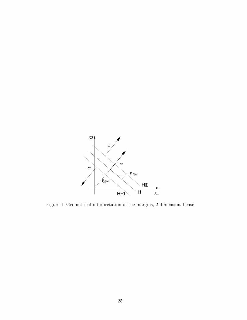
the zero weight vector as a minimizer of (5), see [18, 5].The situation of the criterion function is depicted in fig. 1. In addition to

the original hyperplane H : w · x = 0, there exist two margin hyperplanesH+1 : w · x − ǫ = 0 and H−1 : −w · x − ǫ = 0. The hyperplane H+1 isnow responsible for the classification of the class +1 examples, whereas H−1

is responsible for class −1 ones. Because H+1 is shifted into the class +1region, it causes at least as many errors for class +1 as H does. For class −1the corresponding holds.

It is relatively easy to see that Iǫ is a convex function by considering theconvex function h(z) := k zσ(z) (where k is some constant), and the sumand composition of convex functions. From the convexity of Iǫ it follows thatthere exists a unique minimum value.

It can be shown that the choice of an ǫ > 0 is not critical, because thehyperplanes minimizing the criterion function are identical with respect tothe empirical risk for every ǫ > 0, see also [7].

3.2 The Learning Rule

By differentiating the criterion function Iǫ, we derive the learning rule. Thegradient of Iǫ is given by

∇wIǫ(w) =1

l

∑

(x,c)∈S+1

−c xσ(−w · x + ǫ) +∑

(x,c)∈S−1

c xσ(w · x + ǫ)

(6)

To handle the points, in which Iǫ cannot be differentiated, in [18] the gradientin (6) is considered to be a subgradient. For a subgradient a in a point w, thecondition Iǫ(w

′) ≥ Iǫ(w)+a · (w′−w) for all w′ is required. The subgradientis defined for convex functions, and can be used for incremental learning andstochastic approximation (see [18, 2, 16]).

Considering the gradient for a single example, the following incrementalrule can be derived. For learning, we start with an arbitrary initialisationw(0). The following weight update rule is used when encountering an example(x, y) with cost c at time (learning step) t:

w(t + 1) =

w(t) + γtc x if y = +1 andw(t) · x − ǫ ≤ 0

w(t) − γtc x if y = −1 andw(t) · x + ǫ ≥ 0

w(t) else

(7)

8

We assume either a randomized or a cyclic presentation of the training ex-amples.

In order to guarantee convergence to a minimum and to prevent oscilla-tions, for the factors γt the following conditions for stochastic approximationare imposed: limt→∞ γt = 0,

∑∞t=0 γt = ∞,

∑∞t=0 γ2

t < ∞. A possible choiceis γt = 1

t. The convergence to an optimum in the separable and the non-

separable case follows from the results in [16].If the cost value c is negative due to noise in the data, the example could

just be ignored. This corresponds to modifying the density p(x, y, c) which isin general not desirable. Alternatively, the learning rule (7) must be modifiedin order to misclassify the current example. This can be achieved by using themodified update conditions sign(c)w(t) · x− ǫ ≤ 0 and sign(c)w(t) · x+ ǫ ≥ 0in (7). This means that an example with negative cost is treated as if itbelongs to the other class.

4 Multiple and Disjunctive Classes

In order to deal with multi-class/multimodal problems (e.g. XOR), we haveextended the learning system DIPOL [15, 17, 20] in order to handle exampledependent costs.

The aim of the STATLOG project (see [15]) was the comparison of severalalgorithms from the fields of machine learning, statistical classification andneural networks (excluding SVMs). DIPOL turned out to be one of the mostsuccessful learning algorithms – it performed best on average on all datasets(see [20] for more details).

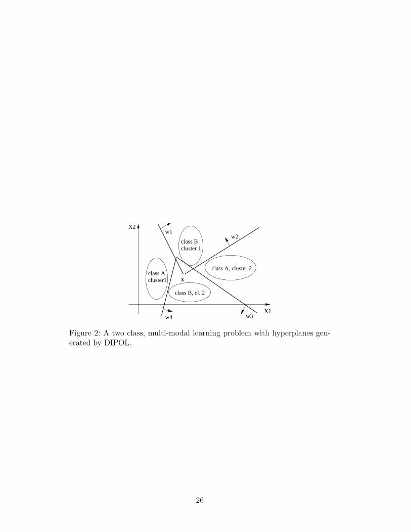
DIPOL can be seen as an extension of the perceptron approach to multipleclasses and multi-modal distributions. A learning problem with two classes,where both classes have a bimodal distribution (i.e. there exist two clusters),is shown in fig. 2 (together with the hyperplanes learned by DIPOL). If aclass possesses a multi-modal distribution (disjunctive classes), the clustersare determined by DIPOL in a preprocessing step using a minimum-varianceclustering algorithm (see [17, 5]) for every class.

In the case of N ≥ 2 classes, each example is described by an N -placecost vector describing the N −1 possibilities of misclassification and the costfor correct classification.

After the (optional) clustering of the classes, a separating hyperplane isconstructed for each pair of classes or clusters if they belong to differentclasses. When creating a hyperplane for a pair of classes or clusters, respec-tively, all examples belonging to other classes/clusters are not taken intoaccount. Of course, for clusters originating from the same class in the train-

9

ing set, no hyperplane has to be constructed.The construction of a hyperplane for a pair of clusters or classes has

two phases. In the weight initialization phase, a least squares problem issolved using standard regression techniques. To one of the classes, the targetvalue +1 is assigned, whereas the other class has the target value −1. Theweights of the regression hyperplane are used as initial values for the secondphase in which a gradient descent is performed. In contrast to the approachdescribed in section 3.2, DIPOL uses a sequence of γt that tends to zero inan exponential manner, yielding a much faster convergence and also goodlearning results because of the in general good initialization of the weightsby the regression step.

After the construction of the hyperplanes, the whole feature space is di-vided into decision regions each belonging to a single class, or cluster respec-tively. For classification of a new example x, it is determined in which regionof the feature space it lies, i.e. a region belonging to a cluster of a class y.The class y of the respective region defined by a subset of the hyperplanes isthe classification result for x.

DIPOL can be trained using the criterion function Iǫ or using a quadraticerror function, e.g. [15, 17, 20]. It incorporates incremental gradient descent(sect. 3.2) as well as a modified batch mode procedure, where the learningrate decays exponentially.

In the new version of DIPOL, example dependent costs can be includedin every step:

• In the clustering step, the costs can be used as an additional attribute,possibly yielding a finer clustering of the data.

• In the regression step, the costs are used as target values. For the class,that is considered to be the −1-class, the costs are multiplied by −1. Inthe case of N > 2 classes, the appropriate entries of the cost vector areconsidered.

• In the gradient descent phase, the costs are incorporated as describedin section 3.2.

In the next section, an alternative approach for the cost-sensitive constructionof linear hyperplanes is considered.

10

5 Support Vector Machines

5.1 SVMs with Example Dependent Costs

DIPOL constructs a classifier by dividing the given input space into regionsbelonging to different classes. The classes are separated by hyperplanes com-puted with the algorithm in sect. 3. In the SVM approach, hyperplanes arenot computed by gradient descent but by directly solving an optimizationproblem, see below. More complex classifiers are formed by an implicit trans-formation of the given input space into a so called feature space by usingkernel functions.

Given a training sample (x(1), y(1), c(1)), . . . , (x(l), y(l), c(l)), the optimiza-tion problem of a standard soft margin support vector machine (SVM) [19, 3]can be stated as

minw,b,ξξξ

1

2|w|2 + C

l∑

i=1

ξki

s.t.y(i)

(w · x(i) + b

)≥ 1 − ξi

ξi ≥ 0,

(8)

where the regularization constant C > 0 determines the trade-off betweenthe complexity term 1

2|w|2 and the sum. It holds that b = −θ. The sum

takes all examples into account for which the corresponding pattern x(i) hasa geometrical margin of less than 1

|w|, and a functional margin of less than 1.

For such an example, the slack variable ξi > 0 denotes the difference to therequired functional margin. Different values of k lead to different versions ofthe soft margin SVM, see e.g. [3].

For k=1, the sum of the ξi can be seen as an upper bound of the empiricalrisk. Hence we can extend the optimization problem (8) in a natural way byweighting the slack variables ξi with the corresponding costs c(i). This leadsfor k = 1 to the cost-sensitive optimization problem2

minw,b,ξξξ

1

2|w|2 + C

l∑

i=1

c(i) ξi

s.t.y(i)

(w · x(i) + b

)≥ 1 − ξi

ξi ≥ 0.

(9)

Introducing non-negative Lagrangian multipliers αi, µi ≥ 0, i = 1, . . . , l, wecan rewrite the optimization problem (9), and obtain the following primal

2A similar approach is taken in [9] for modeling concept drift. There, the weightscorrespond to the recency of the examples.

11

Lagrangian

LP (w, b, ξξξ,ααα,µµµ) =1

2|w|2 + C

l∑

i=1

c(i) ξi

−l∑

i=1

αi

[y(i)

(w · x(i) + b

)−1 + ξi

]−

l∑

i=1

µi ξi.

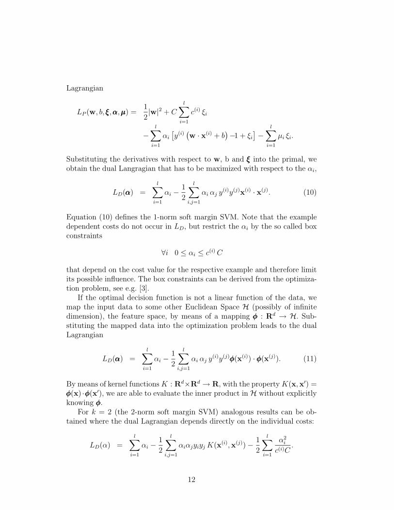
Substituting the derivatives with respect to w, b and ξξξ into the primal, weobtain the dual Langragian that has to be maximized with respect to the αi,

LD(ααα) =l∑

i=1

αi −1

2

l∑

i,j=1

αi αj y(i)y(j)x(i) · x(j). (10)

Equation (10) defines the 1-norm soft margin SVM. Note that the exampledependent costs do not occur in LD, but restrict the αi by the so called boxconstraints

∀i 0 ≤ αi ≤ c(i) C

that depend on the cost value for the respective example and therefore limitits possible influence. The box constraints can be derived from the optimiza-tion problem, see e.g. [3].

If the optimal decision function is not a linear function of the data, wemap the input data to some other Euclidean Space H (possibly of infinitedimension), the feature space, by means of a mapping φφφ : Rd → H. Sub-stituting the mapped data into the optimization problem leads to the dualLagrangian

LD(ααα) =l∑

i=1

αi −1

2

l∑

i,j=1

αi αj y(i)y(j)φφφ(x(i)) · φφφ(x(j)). (11)

By means of kernel functions K : Rd×Rd → R, with the property K(x,x′) =φφφ(x) ·φφφ(x′), we are able to evaluate the inner product in H without explicitlyknowing φφφ.

For k = 2 (the 2-norm soft margin SVM) analogous results can be ob-tained where the dual Lagrangian depends directly on the individual costs:

LD(α) =l∑

i=1

αi −1

2

l∑

i,j=1

αiαjyiyj K(x(i),x(j)) −1

2

l∑

i=1

α2i

c(i)C.

12

5.2 Relation to perceptron learning

In order to show the relationship between the criterion function Iǫ in (5)and the learning problem of the SVM consider the case k = 1. In the limitC → ∞ the sum of the ξi of the objective function is minimized. By meansof the non-negativity function (·)+, with (u)+ = u if u > 0 and (u)+ = 0otherwise, both constraints can be integrated into the single inequality

ξi ≥(1 − y(i)

[w · x(i) + b

])

+(12)

=(1 − y(i)

[w · x(i) + b

])σ

(1 − y(i)

[w · x(i) + b

]), (13)

where we used (u)+ = uσ(u) in order to indicate classification errors. Notethat equality in (12) holds for all patterns. Substituting (13) into the term

l∑

i=1

c(i) ξi of the objective function leads to the minimization problem

minw,b

l∑

i=1

c(i)(1 − y(i)

[w · x(i) + b

])σ

(1 − y(i)

[w · x(i) + b

]). (14)

Using the sets S±1 and the extended vectors w and x equation (14) becomes

minw,b

∑

(x,c)∈S+1

c (−w · x + 1) σ (−w · x + 1) +∑

(x,c)∈S−1

c (w · x + 1) σ (w · x + 1) ,

which is equivalent to the Iǫ criterion function in (5) with ǫ = 1.

5.3 Convergence

Lin showed in [12] that the 2-norm SVM approximates the Bayes rule in thelimit l → ∞. For that purpose he treats the SVM optimization problem asthe following regularization problem in a reproducing kernel Hilbert space(RKHS) HK

minh,b,ξ

1

l

l∑

i=1

ξ2i + λ|h|2HK

s.t. ξi ≥ 1 − y(i)f(x(i))ξi ≥ 0,

with f(x) = h(x)+b and an appropriate trade-off λ = 12lC

. The correspondingregularization problem with example dependent costs can be stated as

minh,b,ξ

1

l

l∑

i=1

c(i) (1 − y(i)f(x(i))︸ ︷︷ ︸

≡ξi

)2+ + λ‖h‖2

HK, (15)

13

where we integrated the constraints by means of the non-negativity function(·)+ into a single inequality which is substituted into the objective function.

In the limit l → ∞ the upper bound of the empirical risk in (15) convergesto the expectation

EX,Y

[cY (X)(1 − Y f(X))2

+

], (16)

where we introduced random variables X and Y . Minimizing EY [·] of theequivalent expression

EX

[EY [cY (X)(1 − Y f(X))2

+|X]]

for every fixed X = x leads to the minimization of

g = c−1(x)(1 + f(x))2+ p(−1|x) + c+1(x)(1 − f(x))2

+ p(+1|x), (17)

with cy′(x(i)) = c(i) if y′ = y(i) and 0 otherwise.It can be shown that the range of the optimal function lies in the interval

f opt(x) ∈ [−1, +1]. Therefore (17) remains non-negative for all x and wecan drop the non-negativity function (·)+. By setting z := f(x) and solving∂g

∂z= 0, we derive the optimal decision function

f opt(x) =c+1(x)p(+1|x) − c−1(x)p(−1|x)

c+1(x)p(+1|x) + c−1(x)p(−1|x).

Proposition 5.1 In the case k = 2, sign(f opt(x)) is a minimizer of R, andit minimizes (16). Moreover it holds

sign(f opt) ≡ r∗.

where r∗ is defined in eq. (3).

Therefore we conjecture from proposition 5.1 that SVM learning approxi-mates the Bayes rule for large training sets. For k = 1 the correspondingcannot be shown.

6 Re-Sampling

Example dependent costs can be included into a cost-insensitive learningalgorithm by re-sampling the given training set. First we define the meancosts for each class by

cy =

∫

Rd

cy(x)p(x|y)dx . (18)

14

We define the global mean cost b = c+1P (+1) + c−1P (−1). From the cost-sensitive definition of the risk in (1) it follows that

R(r)

b=

∫

X+1

c−1(x)p(x|−1)

c−1

c−1P (−1)

bdx

+

∫

X−1

c+1(x)p(x|+1)

c+1

c+1P (+1)

bdx.

This means that we now consider the new class conditional densities

p′(x|y) =1

cy

cy(x)p(x|y)

derived from the compound density

p′(x, y) = p′(x|y)P ′(y) =cy(x)

bp(x, y). (19)

and the new priors

P ′(y) = P (y)cy

c+1P (+1) + c−1P (−1).

It is easy to see that∫

p′(x|y)dx = 1 holds, as well as P ′(+1) + P ′(−1) = 1.Because b is a constant, minimizing the cost-sensitive risk R(r) is equiv-

alent to minimizing the cost-free risk

R(r)

b= R′(r) =

∫

X+1

p′(x|−1)P ′(−1)dx

+

∫

X−1

p′(x|+1)P ′(+1)dx.

In order to minimize R′, we have to draw a new training sample from thegiven training sample. Assume that a training sample (x(1), y(1), c(1)), . . . ,

(x(l), y(l), c(l)) of size l is given. Let Cy be the total cost for class y in thesample. Based on the given sample, we form a second sample of size lN byrandom sampling from the given training set, where N > 0 is a fixed realnumber.

Because of (19), in each of the ⌊lN⌋ independent sampling steps, theprobability of including example i in this step into the new sample should bedetermined by

c(i)

C+1 + C−1

15

i.e. an example is chosen according to its contribution to the total cost of thefixed training set. Note that C+1+C−1

l≈ b holds. Because of R(r) = bR′(r),

it holds Remp(r) ≈ bR′emp(r), where Remp is evaluated with respect to the

given sample, and R′emp(r) is evaluated with respect to the generated cost-

free sample. This means that a learning algorithm that tries to minimize theexpected cost-free risk by minimizing the mean cost-free risk will minimizethe expected cost for the original problem. From the new training set, aclassifier for the cost-sensitive problem can be learned with a cost-insensitivelearning algorithm.

Our approach is related to the resampling approach for class dependentcosts described e.g. in [1], and to the extension of the METACOST-approachfor example dependent costs [22]. We will compare their performances infuture experiments.

7 Experiments

7.1 The uni-modal case

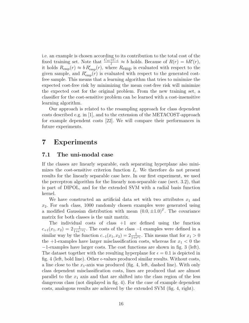
If the classes are linearly separable, each separating hyperplane also mini-mizes the cost-sensitive criterion function Iǫ. We therefore do not presentresults for the linearly separable case here. In our first experiment, we usedthe perceptron algorithm for the linearly non-separable case (sect. 3.2), thatis part of DIPOL, and for the extended SVM with a radial basis functionkernel.

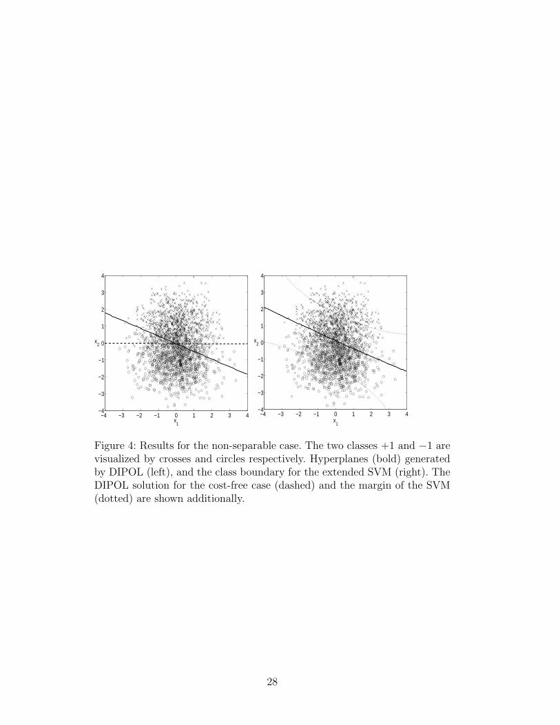
We have constructed an artificial data set with two attributes x1 andx2. For each class, 1000 randomly chosen examples were generated usinga modified Gaussian distribution with mean (0.0,±1.0)T . The covariancematrix for both classes is the unit matrix.

The individual costs of class +1 are defined using the functionc+1(x1, x2) = 2 1

1+e−x1. The costs of the class −1 examples were defined in a

similar way by the function c−1(x1, x2) = 2 11+ex1

. This means that for x1 > 0the +1-examples have larger misclassification costs, whereas for x1 < 0 the−1-examples have larger costs. The cost functions are shown in fig. 3 (left).The dataset together with the resulting hyperplane for ǫ = 0.1 is depicted infig. 4 (left, bold line). Other ǫ-values produced similar results. Without costs,a line close to the x1-axis was produced (fig. 4, left, dashed line). With onlyclass dependent misclassification costs, lines are produced that are almostparallel to the x1 axis and that are shifted into the class region of the lessdangerous class (not displayed in fig. 4). For the case of example dependentcosts, analogous results are achieved by the extended SVM (fig. 4, right).

16

Our selection of the individual cost functions caused a rotation of theclass boundary, see fig. 4. This effect cannot be reached using cost matricesalone. Our approach is therefore a genuine extension of previous approachesfor including costs, which rely on class dependent costs or cost matrices.

7.2 The multi-modal case

For the multi-modal case, we have created the artificial dataset that is shownin fig. 5. Each class consists of two modes, each defined by a Gaussian dis-tribution.

For class +1, we have chosen a constant cost c+1(x1, x2) = 1.0. For class−1 we have chosen a variable cost, that depends only on the x1-value, namelyc−1(x1, x2) = 2 1

1+e−x1. This means, that the examples of the left cluster of

class −1 (with x1 < 0) have smaller costs compared to the class +1 examples,and the examples of the right cluster (with x1 > 0) have larger costs. Thecost functions are shown in fig. 3 (right).

For learning, the augmented version of DIPOL was provided with the2000 training examples together with their individual costs. The result of thelearning algorithm is displayed in fig. 5. For reasons of symmetry, the sep-arating hyperplanes that would be generated without individual costs mustcoincide with one of the bisecting lines of the coordinate system. It is obvi-ous in fig. 5, that this is not the case for the hyperplanes that DIPOL hasproduced for the dataset with the individual costs: The left region of class−1 is a little bit smaller, the right region is a little bit larger compared tolearning without costs. Both results are according to the intuition.

The solution of the extended SVM with a radial basis function kernelresults in the same shift of the class regions. Due to a higher sensitivity tooutliers the decision boundary is curved in contrast to the piecewise linearhyperplanes generated by DIPOL.

7.3 German Credit Data Set

In order to apply our approach to a real world domain, we also conductedexperiments on the German Credit Data Set ([15], chapter 9) from the STAT-LOG project (the dataset can be downloaded from the UCI repository). Thedata set has 700 examples of class “good customer” (class +1) and 300 ex-amples of class ”bad customer” (class −1). Each example is described by24 attributes. Because the data set does not come with example dependentcosts, we assumed the following cost model: If a good customer is incorrectly

classified as a bad customer, we assumed the cost of 0.1duration12

· amount,where duration is the duration of the credit in months, and amount is the

17

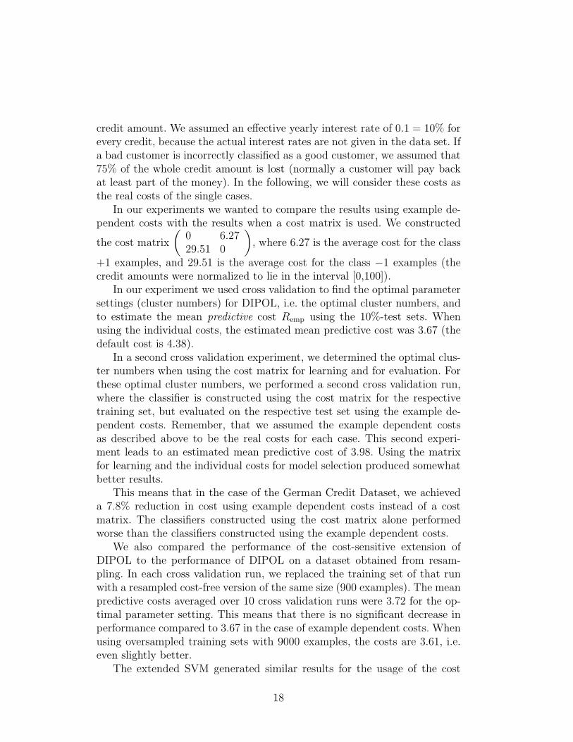
credit amount. We assumed an effective yearly interest rate of 0.1 = 10% forevery credit, because the actual interest rates are not given in the data set. Ifa bad customer is incorrectly classified as a good customer, we assumed that75% of the whole credit amount is lost (normally a customer will pay backat least part of the money). In the following, we will consider these costs asthe real costs of the single cases.

In our experiments we wanted to compare the results using example de-pendent costs with the results when a cost matrix is used. We constructed

the cost matrix

(0 6.2729.51 0

)

, where 6.27 is the average cost for the class

+1 examples, and 29.51 is the average cost for the class −1 examples (thecredit amounts were normalized to lie in the interval [0,100]).

In our experiment we used cross validation to find the optimal parametersettings (cluster numbers) for DIPOL, i.e. the optimal cluster numbers, andto estimate the mean predictive cost Remp using the 10%-test sets. Whenusing the individual costs, the estimated mean predictive cost was 3.67 (thedefault cost is 4.38).

In a second cross validation experiment, we determined the optimal clus-ter numbers when using the cost matrix for learning and for evaluation. Forthese optimal cluster numbers, we performed a second cross validation run,where the classifier is constructed using the cost matrix for the respectivetraining set, but evaluated on the respective test set using the example de-pendent costs. Remember, that we assumed the example dependent costsas described above to be the real costs for each case. This second experi-ment leads to an estimated mean predictive cost of 3.98. Using the matrixfor learning and the individual costs for model selection produced somewhatbetter results.

This means that in the case of the German Credit Dataset, we achieveda 7.8% reduction in cost using example dependent costs instead of a costmatrix. The classifiers constructed using the cost matrix alone performedworse than the classifiers constructed using the example dependent costs.

We also compared the performance of the cost-sensitive extension ofDIPOL to the performance of DIPOL on a dataset obtained from resam-pling. In each cross validation run, we replaced the training set of that runwith a resampled cost-free version of the same size (900 examples). The meanpredictive costs averaged over 10 cross validation runs were 3.72 for the op-timal parameter setting. This means that there is no significant decrease inperformance compared to 3.67 in the case of example dependent costs. Whenusing oversampled training sets with 9000 examples, the costs are 3.61, i.e.even slightly better.

The extended SVM generated similar results for the usage of the cost

18

matrix and the example dependent costs respectively, i.e. we found no sub-stantially increased performance. The reason is presumably that the resultsfor DIPOL, the SVM, and other learning algorithms are not much betterthan the default rule, see [15], though DIPOL and SVM perform comparablywell.

7.4 The KDD-98 dataset

The KDD-98 dataset [8] contains informations on persons that were mailedduring a campaign with requests to donate to a charity. In the dataset thereare two classes. The first class consists of persons that received a mail butdid not give some money (non-donators). The second class consists of thosepersons that received a mail and spent some money (donators). The learnedclassifier is intended to be used to decide whom to send a request in a futurecampaign.

For a non-donator, the misclassification cost corresponds to the cost ofthe mail that is estimated as $0.68. The cost for correct classification is zerowhich captures the case of deciding not to send a letter. For donators, the costfor misclassification is also set to zero, because in this case no letter wouldhave been sent. The costs (i.e. gain) for correct classification is the donationamount minus the cost for the mail. This value varies between $−0.32 and$−199.32.

For learning with the training set that contains 95413 examples, we useda normalized version of the dataset, as described in section 2 (zero cost forcorrect classification). For testing we used the validation dataset containing96386 examples and the original cost functions giving the estimated totalgain of the future mailing campaign. The default gain when mailing to everyperson is $10560.

Using DIPOL together with example dependent costs, the gain was$12163 while the extended 2-norm SVM with a radial basis function kernelreaches $12374. We also created resampled data from the original dataset.Using this dataset, we achieved an increased gain of $12883 with a ”vanilla”SVM in contrast to $14045 with DIPOL (averaged over 10 resampleddatasets). Note that the latter result is only slightly worse than the win-ner of the KDD-98 competition ($14712).

In [23] slightly better results are reported for a modified sampling strat-egy3 that is combined with averaging classifiers (“costing”). We assume thatour results can be improved too by using a multi-classifier approach. Obvi-ously, the inclusion of duplicates that can occur during resampling does not

3The strategy in [23] was developed independently from ours.

19

play a negative role for DIPOL.We conjecture that for DIPOL the increase in gain is due to the fact that

in the resampled dataset, the two classes are rather balanced in contrast tothe original dataset. Seemingly, this makes learning easier for DIPOL. Firstinvestigations have shown that in the case of the resampled data set, theregression step already produces very accurate hyperplanes. For the originaldataset, this is not always the case.

A general advantage of DIPOL over the resampling strategy is the treat-ment of more than two classes. While DIPOL can be applied in this casewithout problems, there is no straightforward way to extend the resamplingstrategy.

8 Conclusion

In this article we discussed a natural cost-sensitive extension of perceptronlearning with example dependent costs for correct classification and misclas-sification. We stated an appropriate criterion function and derived a cost-sensitive learning rule for linearly non-separable classes from it, that is anatural extension of the cost-insensitive perceptron learning rule for separa-ble classes.

We showed that the Bayes rule only depends on differences between costsfor correct classification and for misclassification. This allows us to define asimplified learning problem where the costs for correct classification are as-sumed to be zero. In addition to costs for correct and incorrect classification,it would be possible to consider example dependent costs for rejection, too.

The usage of example dependent costs instead of class dependent costsleads to a decreased misclassification cost in practical applications, e.g. creditrisk assignment.

Experiments with the extended SVM approach verified the results of per-ceptron learning. Its main advantage lies in a lower error at the expenseof non-interpretable decision boundaries. The piecewise linear classifier ofDIPOL can easily be transformed to disjunctive rules with linear inequali-ties.

With respect to the resampling strategy presented in this paper, we haveshown that it performs well and may even lead to an increased performance.The theoretical properties of the approach have to be investigated in futurework. For example there is the possibility of including duplicates of singleexamples that lead to a bias.

20

Acknowledgments. We thank Bianca Zadrozny for providing a version ofKDD-98 dataset with a reduced number of attributes.

References

[1] P. K. Chan and S. J. Stolfo. Toward scalable learning with non-uniformclass and cost distributions: A case study in credit card fraud detection.In Knowledge Discovery and Data Mining (Proc. KDD98), pages 164–168, 1998.

[2] F. H. Clarke. Optimization and Nonsmooth Analysis. Canadian Math.Soc. Series of Monographs and Advanced Texts. John Wiley & Sons,1983.

[3] N. Cristianini and J. Shawe-Taylor. An Introduction to Support Vec-tor Machines (and Other Kernel-Based Learning Methods). CambridgeUniversity Press, 2000.

[4] L. Devroye, L. Gyorfi, and L. Gabor. A Probabilistic Theory of PatternRecognition. Springer-Verlag, 1996.

[5] R. O. Duda and P. E. Hart. Pattern Classification and Scene Analysis.John Wiley & Sons, New York, 1973.

[6] Charles Elkan. The foundations of Cost-Sensitive learning. In BernhardNebel, editor, Proceedings of the seventeenth International Conferenceon Artificial Intelligence (IJCAI-01), pages 973–978, San Francisco, CA,August 4–10 2001. Morgan Kaufmann Publishers, Inc.

[7] P. Geibel and F. Wysotzki. Using costs varying from object toobject to construct linear and piecewise linear classifiers. Tech-nical Report 2002-5, TU Berlin, Fak. IV (WWW http://ki.cs.tu-berlin.de/∼geibel/publications.html), 2002.

[8] S. Hettich and S.D. Bay. The UCI KDD archive. University of California,Irvine. http://kdd.ics.uci-edu/.

[9] R. Klinkenberg and S. Ruping. Concept drift and the importance ofexamples. In J. Franke, G. Nakhaeizadeh, and I. Renz, editors, TextMining – Theoretical Aspects and Applications. Springer, 2003.

21

[10] M. Kukar and I. Kononenko. Cost-sensitive learning with neural net-works. In Henri Prade, editor, Proceedings of the 13th European Con-ference on Artificial Intelligence (ECAI-98), pages 445–449, Chichester,1998. John Wiley & Sons.

[11] A. Lenarcik and Z. Piasta. Rough classifiers sensitive to costs varyingfrom object to object. In Lech Polkowski and Andrzej Skowron, editors,Proceedings of the 1st International Conference on Rough Sets and Cur-rent Trends in Computing (RSCTC-98), volume 1424 of LNAI, pages222–230, Berlin, June 22–26 1998. Springer.

[12] Y. Lin. Support vector machines and the bayes rule in classification.Data Mining and Knowledge Discovery, 6(3):259–275, 2002.

[13] Y. Lin, Y. Lee, and G. Wahba. Support vector machines for classificationin nonstandard situations. Machine Learning, 46(1-3):191–202, 2002.

[14] D. D. Margineantu and T. G. Dietterich. Bootstrap methods for thecost-sensitive evaluation of classifiers. In Proc. 17th International Conf.on Machine Learning, pages 583–590. Morgan Kaufmann, San Francisco,CA, 2000.

[15] D. Michie, D. H. Spiegelhalter, and C. C. Taylor. Machine Learning,Neural and Statistical Classification. Series in Artificial Intelligence. EllisHorwood, 1994.

[16] A. Nedic and D.P. Bertsekas. Incremental subgradient methods for non-differentiable optimization. SIAM Journal on Optimization, pages 109–138, 2001.

[17] B. Schulmeister and F. Wysotzki. Dipol - a hybrid piecewise linearclassifier. In R. Nakeiazadeh and C. C. Taylor, editors, Machine Learningand Statistics: The Interface, pages 133–151. Wiley, 1997.

[18] S. Unger and F. Wysotzki. Lernfahige Klassifizierungssysteme (Classi-fier Systems that are able to Learn). Akademie-Verlag, Berlin, 1981.

[19] V. N. Vapnik. The Nature of Statistical Learning Theory. Springer, NewYork, 1995.

[20] F. Wysotzki, W. Muller, and B. Schulmeister. Automatic constructionof decision trees and neural nets for classification using statistical consid-erations. In G. DellaRiccia, H.-J. Lenz, and R. Kruse, editors, Learning,Networks and Statistics, number 382 in CISM Courses and Lectures.Springer, 1997.

22

[21] J. Yang, R. Parekh, and V. Honavar. Comparison of performance ofvariants of single-layer perceptron algorithms on non-separable data.Neural, Parallel and Scientific Computation, 8:415–438, 2000.

[22] B. Zadrozny and C. Elkan. Learning and making decisions when costsand probabilities are both unknown. In Foster Provost and Ramakrish-nan Srikant, editors, Proceedings of the Seventh ACM SIGKDD Interna-tional Conference on Knowledge Discovery and Data Mining (KDD-01),pages 204–214, New York, August 26–29 2001. ACM Press.

[23] B. Zadrozny, J. Langford, and N. Abe. Cost-sensitive learning by cost-proportionate example weighting. In Proceedings of the 2003 IEEE In-ternational Conference on Data Mining, 2003. to appear.

23

List of Figures

1 Geometrical interpretation of the margins, 2-dimensional case 252 A two class, multi-modal learning problem with hyperplanes

generated by DIPOL. . . . . . . . . . . . . . . . . . . . . . . . 263 Cost functions in the non-separable case (left), and the multi-

modal case (right). . . . . . . . . . . . . . . . . . . . . . . . . 274 Results for the non-separable case. The two classes +1 and −1

are visualized by crosses and circles respectively. Hyperplanes(bold) generated by DIPOL (left), and the class boundary forthe extended SVM (right). The DIPOL solution for the cost-free case (dashed) and the margin of the SVM (dotted) areshown additionally. . . . . . . . . . . . . . . . . . . . . . . . . 28

5 Results for the multi-modal non-separable case. Bold lines vi-sualize the learned hyperplanes by DIPOL (left) and the ex-tended SVM (right). . . . . . . . . . . . . . . . . . . . . . . . 29

24

Η−1

Η+1Η

θ/|w|

/|w|

-w

w

w

X1

X2

ε

Figure 1: Geometrical interpretation of the margins, 2-dimensional case

25

X2

X1

cluster1

cluster 1

w1w2

w3w4

xclass A

class A, cluster 2

class B

class B, cl. 2

Figure 2: A two class, multi-modal learning problem with hyperplanes gen-erated by DIPOL.

26

c1(x_1,x_2)c-1(x_1,x_2)

-4 -3 -2 -1 0 1 2 3 4x1-4

-3-2

-10

12

34

x2

0

0.5

1

1.5

2

c+1(x_1,x_2)c-1(x_1,x_2)

-4 -3 -2 -1 0 1 2 3 4x1-4

-3-2

-10

12

34

x2

0

0.5

1

1.5

2

Figure 3: Cost functions in the non-separable case (left), and the multi-modalcase (right).

27

−4 −3 −2 −1 0 1 2 3 4−4

−3

−2

−1

0

1

2

3

4

x1

x2

−4 −3 −2 −1 0 1 2 3 4−4

−3

−2

−1

0

1

2

3

4

x1

x2

Figure 4: Results for the non-separable case. The two classes +1 and −1 arevisualized by crosses and circles respectively. Hyperplanes (bold) generatedby DIPOL (left), and the class boundary for the extended SVM (right). TheDIPOL solution for the cost-free case (dashed) and the margin of the SVM(dotted) are shown additionally.

28

−4 −3 −2 −1 0 1 2 3 4−4

−3

−2

−1

0

1

2

3

4

X1

X2

−4 −3 −2 −1 0 1 2 3 4−4

−3

−2

−1

0

1

2

3

4

x1

x2

Figure 5: Results for the multi-modal non-separable case. Bold lines visualizethe learned hyperplanes by DIPOL (left) and the extended SVM (right).

29