perceptual and sensory augmented computing computer vision ws 11/12 computer vision – lecture 9...
TRANSCRIPT

Perc
ep
tual an
d S
en
sory
Au
gm
en
ted
Com
pu
tin
gC
om
pu
ter
Vis
ion
WS
11
/12
Computer Vision – Lecture 9Subspace Representations for
Recognition
24.11.2011
Bastian LeibeRWTH Aachenhttp://www.mmp.rwth-aachen.de/

Perc
ep
tual an
d S
en
sory
Au
gm
en
ted
Com
pu
tin
gC
om
pu
ter
Vis
ion
WS
11
/12
Course Outline
• Image Processing Basics• Segmentation & Grouping• Recognition
Global Representations Subspace representations
• Object Categorization I Sliding Window based Object Detection
• Local Features & Matching• Object Categorization II
Part based Approaches
• 3D Reconstruction• Motion and Tracking
2
Perc
ep
tual an
d S
en
sory
Au
gm
en
ted
Com
pu
tin
gC
om
pu
ter
Vis
ion
WS
11
/12
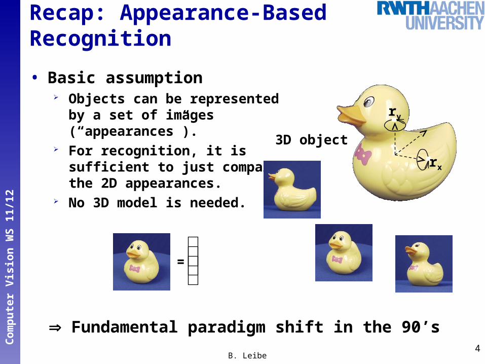
Recap: Appearance-Based Recognition
• Basic assumption Objects can be represented
by a set of images(“appearances”).
For recognition, it is sufficient to just comparethe 2D appearances.
No 3D model is needed.
4
3D object
ry
rx
Fundamental paradigm shift in the 90’s
B. Leibe
=

Perc
ep
tual an
d S
en
sory
Au
gm
en
ted
Com
pu
tin
gC
om
pu
ter
Vis
ion
WS
11
/12
Recap: Recognition Using Histograms
• Histogram comparison
5B. Leibe
Test image
Known objects

Perc
ep
tual an
d S
en
sory
Au
gm
en
ted
Com
pu
tin
gC
om
pu
ter
Vis
ion
WS
11
/12
Recap: Comparison Measures
• Vector space interpretation Euclidean distance Mahalanobis distance
• Statistical motivation Chi-square Bhattacharyya
• Information-theoretic motivation Kullback-Leibler divergence, Jeffreys divergence
• Histogram motivation Histogram intersection
• Ground distance Earth Movers Distance (EMD)
6
≠

Perc
ep
tual an
d S
en
sory
Au
gm
en
ted
Com
pu
tin
gC
om
pu
ter
Vis
ion
WS
11
/12
Recap: Recognition Using Histograms
• Simple algorithm1. Build a set of histograms H={hi} for each known
object More exactly, for each view of each object
2. Build a histogram ht for the test image.
3. Compare ht to each hiH Using a suitable comparison measure
4. Select the object with the best matching score Or reject the test image if no object is similar enough.
7
“Nearest-Neighbor” strategy
B. Leibe

Perc
ep
tual an
d S
en
sory
Au
gm
en
ted
Com
pu
tin
gC
om
pu
ter
Vis
ion
WS
11
/12
Recap: Histogram Backprojection
• „Where in the image are the colors we‘re looking for?“
Query: object with histogram M Given: image with histogram I
• Compute the „ratio histogram“: R reveals how important an object
color is, relative to the current image. Project value back into the image (i.e. replace the
image values by the values of R that they index). Convolve result image with a circular mask to find
the object.
8

Perc
ep
tual an
d S
en
sory
Au
gm
en
ted
Com
pu
tin
gC
om
pu
ter
Vis
ion
WS
11
/12
Recap: Multidimensional Representations
• Combination of several descriptors Each descriptor is
applied to the whole image.
Corresponding pixel valuesare combined into one feature vector.
Feature vectors are collectedin multidimensional histogram.
9
Dx
Dy
Lap
1.22-0.392.78
B. Leibe

Perc
ep
tual an
d S
en
sory
Au
gm
en
ted
Com
pu
tin
gC
om
pu
ter
Vis
ion
WS
11
/12
1. Build up histograms p(mk|on) for each training object.
2. Sample the test image to obtain mk, kK. Only small number of local samples necessary.
3. Compute the probabilities for each training object.
4. Select the object with the highest probability Or reject the test image if no object accumulates sufficient
probability.
Recap: Bayesian Recognition Algorithm
10B. Leibe

Perc
ep
tual an
d S
en
sory
Au
gm
en
ted
Com
pu
tin
gC
om
pu
ter
Vis
ion
WS
11
/12
Recap: Colored Derivatives
• Generalization: derivatives along Y axis intensity differences C1 axis red-green differences C2 axis blue-yellow differences
• Application: Brand identification in video
11[Hall & Crowley, 2000]B. Leibe
Y
C2
C1

Perc
ep
tual an
d S
en
sory
Au
gm
en
ted
Com
pu
tin
gC
om
pu
ter
Vis
ion
WS
11
/12
Topics of This Lecture
• Subspace Methods for Recognition Motivation
• Principal Component Analysis (PCA) Derivation Object recognition with PCA Eigenimages/Eigenfaces Limitations
• Fisher’s Linear Discriminant Analysis (FLD/LDA)
Derivation Fisherfaces for recognition
13B. Leibe

Perc
ep
tual an
d S
en
sory
Au
gm
en
ted
Com
pu
tin
gC
om
pu
ter
Vis
ion
WS
11
/12
Representations for Recognition
• Global object representations We’ve seen histograms as one example What could be other suitable
representations?
• More generally, we want to obtain representations that are well-suited for
Recognizing a certain class of objects Identifying individuals from that class (identification)
• How can we arrive at such a representation?
• Approach 1: Come up with a brilliant idea and tweak it until it works.
• Can we do this more systematically?14
B. Leibe

Perc
ep
tual an
d S
en
sory
Au
gm
en
ted
Com
pu
tin
gC
om
pu
ter
Vis
ion
WS
11
/12
Example: The Space of All Face Images
• When viewed as vectors of pixel values, face images are extremely high-dimensional.
100x100 image = 10,000 dimensions
• However, relatively few 10,000-dimensional vectors correspond to valid face images.
• We want to effectively model the subspace of face images.
15B. LeibeSlide credit: Svetlana Lazebnik

Perc
ep
tual an
d S
en
sory
Au
gm
en
ted
Com
pu
tin
gC
om
pu
ter
Vis
ion
WS
11
/12
The Space of All Face Images
• We want to construct a low-dimensional linear subspace that best explains the variation in the set of face images
16B. LeibeSlide credit: Svetlana Lazebnik
Perc
ep
tual an
d S
en
sory
Au
gm
en
ted
Com
pu
tin
gC
om
pu
ter
Vis
ion
WS
11
/12
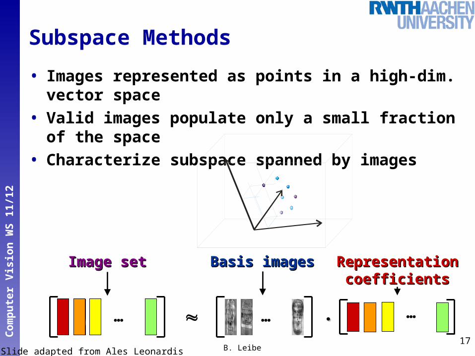
Subspace Methods
• Images represented as points in a high-dim. vector space
• Valid images populate only a small fraction of the space
• Characterize subspace spanned by images
17B. LeibeSlide adapted from Ales Leonardis
… … … ..
Image setImage set Basis imagesBasis images RepresentationRepresentationcoefficientscoefficients

Perc
ep
tual an
d S
en
sory
Au
gm
en
ted
Com
pu
tin
gC
om
pu
ter
Vis
ion
WS
11
/12
Subspace Methods
• Today’s topics: PCA, FLD18
B. Leibe
Subspace Subspace methodsmethods
ReconstructiReconstructiveve
DiscriminativDiscriminativee
PCAPCA, ICA, , ICA, NMFNMF
FLDFLD, SVM, , SVM, CCACCA
= +a= +a11 +a +a22 +a+a3 3 ++ ……
representatirepresentationon
classificaticlassificationon
regressionregression
Slide credit: Ales Leonardis

Perc
ep
tual an
d S
en
sory
Au
gm
en
ted
Com
pu
tin
gC
om
pu
ter
Vis
ion
WS
11
/12
Topics of This Lecture
• Subspace Methods for Recognition Motivation
• Principal Component Analysis (PCA) Derivation Object recognition with PCA Eigenimages/Eigenfaces Limitations
• Fisher’s Linear Discriminant Analysis (FLD/LDA)
Derivation Fisherfaces for recognition
19B. Leibe

Perc
ep
tual an
d S
en
sory
Au
gm
en
ted
Com
pu
tin
gC
om
pu
ter
Vis
ion
WS
11
/12
Principal Component Analysis
• Given: N data points x1, … ,xN in Rd
• We want to find a new set of features that are linear combinations of original ones:
(¹: mean of data points)
• What unit vector u in Rd captures the most variance of the data?
20B. LeibeSlide credit: Svetlana Lazebnik
u(xi ) = u>(xi ¡ ¹ )

Perc
ep
tual an
d S
en
sory
Au
gm
en
ted
Com
pu
tin
gC
om
pu
ter
Vis
ion
WS
11
/12
Principal Component Analysis
• Direction that maximizes the variance of the projected data:
The direction that maximizes the variance is the eigenvector associated with the largest eigenvalue of .
21B. Leibe
Projection of data point
Covariance matrix of data
N
N
Slide credit: Svetlana Lazebnik
1
N
1
N

Perc
ep
tual an
d S
en
sory
Au
gm
en
ted
Com
pu
tin
gC
om
pu
ter
Vis
ion
WS
11
/12
Remember: Fitting a Gaussian
• Mean and covariance matrix of data define a Gaussian model
22
g
1g
2g

Perc
ep
tual an
d S
en
sory
Au
gm
en
ted
Com
pu
tin
gC
om
pu
ter
Vis
ion
WS
11
/12
Interpretation of PCA
• Compute eigenvectors of covariance §. • Eigenvectors: main directions• Eigenvalues: variances along eigenvector
• Result: coordinate transform to best represent the variance of the data
23
u1u2
¹
x2
x1

Perc
ep
tual an
d S
en
sory
Au
gm
en
ted
Com
pu
tin
gC
om
pu
ter
Vis
ion
WS
11
/12
Interpretation of PCA
• Now, suppose we want to represent the data using just a single dimension.
I.e., project it onto a single axis What would be the best choice for this axis?
24
u1u2
¹
x2
x1

Perc
ep
tual an
d S
en
sory
Au
gm
en
ted
Com
pu
tin
gC
om
pu
ter
Vis
ion
WS
11
/12
Interpretation of PCA
• Now, suppose we want to represent the data using just a single dimension.
I.e., project it onto a single axis What would be the best choice for this axis?
• The first eigenvector gives us the best reconstruction.
Direction that retains most of the variance of the data.25
u1
¹
x2
x1

Perc
ep
tual an
d S
en
sory
Au
gm
en
ted
Com
pu
tin
gC
om
pu
ter
Vis
ion
WS
11
/12
Properties of PCA
• It can be shown that the mean square error between xi and its reconstruction using only m principle eigenvectors is given by the expression:
where ¸_j are the eigenvalues
• Interpretation PCA minimizes reconstruction error PCA maximizes variance of projection Finds a more “natural” coordinate system for the sample
data.26
B. LeibeSlide credit: Ales Leonardis
Cumulative influenceof eigenvectors
90% of variance
k eigenvectors
NX
j =1
¸ j ¡mX
j =1
¸ j =NX
j =m+1
¸ j

Perc
ep
tual an
d S
en
sory
Au
gm
en
ted
Com
pu
tin
gC
om
pu
ter
Vis
ion
WS
11
/12
Projection and Reconstruction
• An n-pixel image xRn can beprojected to a low-dimensionalfeature space yRm by
• From yRm, the reconstruc-tion of the point is UTy
• The error of the reconstruc-tion is
27B. LeibeSlide credit: Peter Belhumeur
x 2 Rn
y Ux
Tx U Ux

Perc
ep
tual an
d S
en
sory
Au
gm
en
ted
Com
pu
tin
gC
om
pu
ter
Vis
ion
WS
11
/12
Example: Object Representation
28B. LeibeSlide credit: Ales Leonardis

Perc
ep
tual an
d S
en
sory
Au
gm
en
ted
Com
pu
tin
gC
om
pu
ter
Vis
ion
WS
11
/12
Principal Component Analysis
29B. Leibe
= + w1 + w2 + w3
Slide credit: Ales Leonardis
Get a compact representationby keeping only
the first keigenvectors!

Perc
ep
tual an
d S
en
sory
Au
gm
en
ted
Com
pu
tin
gC
om
pu
ter
Vis
ion
WS
11
/12
Object Detection by Distance TO Eigenspace
• Scan a window over the imageand classify the window as objector non-object as follows:
Project window to subspaceand reconstruct as earlier.
Compute the distance bet-ween and the reconstruc-tion (reprojection error).
Local minima of distance overall image locations objectlocations
Repeat at different scales Possibly normalize window intensity
such that ||=1.
30B. LeibeSlide credit: Peter Belhumeur

Perc
ep
tual an
d S
en
sory
Au
gm
en
ted
Com
pu
tin
gC
om
pu
ter
Vis
ion
WS
11
/12
Eigenfaces: Key Idea
• Assume that most face images lie on a low-dimensional subspace determined by the first k (k < d) directions of maximum variance
• Use PCA to determine the vectors u1,…uk that span that subspace:x ≈ μ + w1u1 + w2u2 + … + wkuk
• Represent each face using its “face space” coordinates (w1,…wk)
• Perform nearest-neighbor recognition in “face space”
31B. Leibe
M. Turk and A. Pentland, Face Recognition using Eigenfaces, CVPR 1991Slide credit: Svetlana Lazebnik

Perc
ep
tual an
d S
en
sory
Au
gm
en
ted
Com
pu
tin
gC
om
pu
ter
Vis
ion
WS
11
/12
Eigenfaces Example
• Training imagesx1,…,xN
32B. LeibeSlide credit: Svetlana Lazebnik

Perc
ep
tual an
d S
en
sory
Au
gm
en
ted
Com
pu
tin
gC
om
pu
ter
Vis
ion
WS
11
/12
Eigenfaces Example
33B. Leibe
Top eigenvectors:u1,…uk
Mean: μ
Slide credit: Svetlana Lazebnik

Perc
ep
tual an
d S
en
sory
Au
gm
en
ted
Com
pu
tin
gC
om
pu
ter
Vis
ion
WS
11
/12
Eigenface Example 2 (Better Alignment)
34B. LeibeSlide credit: Peter Belhumeur

Perc
ep
tual an
d S
en
sory
Au
gm
en
ted
Com
pu
tin
gC
om
pu
ter
Vis
ion
WS
11
/12
Eigenfaces Example
• Face x in “face space” coordinates:
35B. Leibe
=
Slide credit: Svetlana Lazebnik

Perc
ep
tual an
d S
en
sory
Au
gm
en
ted
Com
pu
tin
gC
om
pu
ter
Vis
ion
WS
11
/12
Eigenfaces Example
• Face x in “face space” coordinates:
• Reconstruction:
36B. Leibe
=
= +
µ + w1u1 + w2u2 + w3u3 + w4u4 + …x =
Slide credit: Svetlana Lazebnik
Perc
ep
tual an
d S
en
sory
Au
gm
en
ted
Com
pu
tin
gC
om
pu
ter
Vis
ion
WS
11
/12
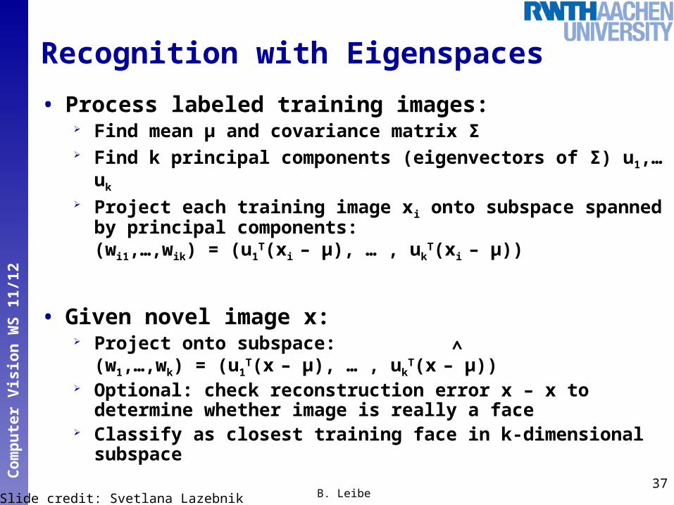
Recognition with Eigenspaces
• Process labeled training images: Find mean µ and covariance matrix Σ Find k principal components (eigenvectors of Σ) u1,…
uk
Project each training image xi onto subspace spanned by principal components:(wi1,…,wik) = (u1
T(xi – µ), … , ukT(xi – µ))
• Given novel image x: Project onto subspace:
(w1,…,wk) = (u1T(x – µ), … , uk
T(x – µ)) Optional: check reconstruction error x – x to
determine whether image is really a face Classify as closest training face in k-dimensional
subspace37
B. LeibeSlide credit: Svetlana Lazebnik
^

Perc
ep
tual an
d S
en
sory
Au
gm
en
ted
Com
pu
tin
gC
om
pu
ter
Vis
ion
WS
11
/12
Obj. Identification by Distance IN Eigenspace
• Objects are represented as coordinates in an n-dim. eigenspace.
• Example: 3D space with points representing individual objects or a
manifold representing parametric eigenspace (e.g., orientation, pose, illumination).
• Estimate parameters by finding the NN in the eigenspace
38B. LeibeSlide credit: Ales Leonardis

Perc
ep
tual an
d S
en
sory
Au
gm
en
ted
Com
pu
tin
gC
om
pu
ter
Vis
ion
WS
11
/12
Parametric Eigenspace
• Object identification / pose estimation Find nearest neighbor in eigenspace [Murase & Nayar,
IJCV’95]39
B. LeibeSlide adapted from Ales Leonardis

Perc
ep
tual an
d S
en
sory
Au
gm
en
ted
Com
pu
tin
gC
om
pu
ter
Vis
ion
WS
11
/12
H. Murase and S. Nayar, Visual learning and recognition of 3-d objects from appearance, IJCV 1995
Applications: Recognition, Pose Estimation

Perc
ep
tual an
d S
en
sory
Au
gm
en
ted
Com
pu
tin
gC
om
pu
ter
Vis
ion
WS
11
/12
Applications: Visual Inspection
41B. Leibe
S. K. Nayar, S. A. Nene, and H. Murase, Subspace Methods for Robot Vision, IEEE Transactions on Robotics and Automation, 1996.
Perc
ep
tual an
d S
en
sory
Au
gm
en
ted
Com
pu
tin
gC
om
pu
ter
Vis
ion
WS
11
/12
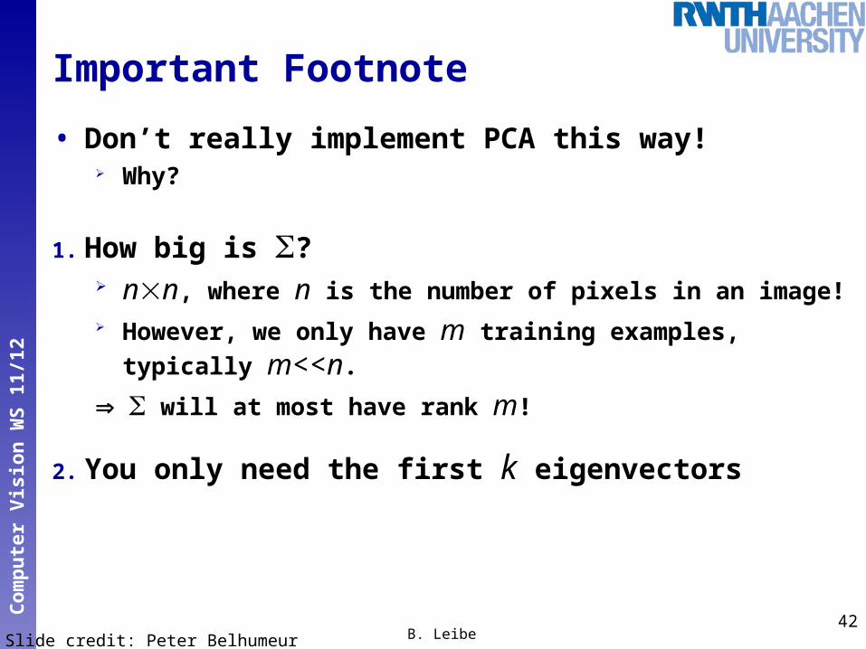
Important Footnote
• Don’t really implement PCA this way! Why?
1. How big is ? nn, where n is the number of pixels in an image! However, we only have m training examples, typically
m<<n.
will at most have rank m!
2. You only need the first k eigenvectors
42B. LeibeSlide credit: Peter Belhumeur

Perc
ep
tual an
d S
en
sory
Au
gm
en
ted
Com
pu
tin
gC
om
pu
ter
Vis
ion
WS
11
/12
Singular Value Decomposition (SVD)
• Any mn matrix A may be factored such that
• U: mm, orthogonal matrix Columns of U are the eigenvectors of AAT
• V: nn, orthogonal matrix Columns are the eigenvectors of ATA
: mn, diagonal with non-negative entries (1, 2,…,
s) with s=min(m,n) are called the singular values. Singular values are the square roots of the eigenvalues of
both AAT and ATA. Columns of U are corresponding eigenvectors!
Result of SVD algorithm: 12…s43
[ ] [ ][ ][ ]
TA U V
m n m m m n n n
Slide credit: Peter Belhumeur

Perc
ep
tual an
d S
en
sory
Au
gm
en
ted
Com
pu
tin
gC
om
pu
ter
Vis
ion
WS
11
/12
SVD Properties
• Matlab: [u s v] = svd(A) where A = u*s*v’
• r = rank(A) Number of non-zero singular values
• U, V give us orthonormal bases for the subspaces of A
first r columns of U: column space of A last m-r columns of U: left nullspace of A first r columns of V: row space of A last n-r columns of V: nullspace of A
• For d r, the first d columns of U provide the best d-dimensional basis for columns of A in least-squares sense
44B. LeibeSlide credit: Peter Belhumeur

Perc
ep
tual an
d S
en
sory
Au
gm
en
ted
Com
pu
tin
gC
om
pu
ter
Vis
ion
WS
11
/12
Performing PCA with SVD
• Singular values of A are the square roots of eigenvalues of both AAT and ATA.
Columns of U are the corresponding eigenvectors.
• And
• Covariance matrix
• So, ignoring the factor 1/n, subtract mean image from each input image, create data matrix , and perform (thin) SVD on the data matrix.
45B. Leibe
1 11
nTT T
i i n ni
a a a a a a AA
Slide credit: Peter Belhumeur
§ =1n
nX
i=1
(~xi ¡ ~¹ )(~xi ¡ ~¹ )T
A = (~xi ¡ ~¹ )

Perc
ep
tual an
d S
en
sory
Au
gm
en
ted
Com
pu
tin
gC
om
pu
ter
Vis
ion
WS
11
/12
Thin SVD
• Any m by n matrix A may be factored such that
• If m>n, then one can view as:
• Where ’=diag(1,2,…,s) with s=min(m,n), and
lower matrix is (n-m by m) of zeros.
• Alternatively, you can write:
• In Matlab, thin SVD is: [U S V] = svds(A,k) 46
B. Leibe
'
0
TA U V
' ' TA U V This is what you
should use!
Slide credit: Peter Belhumeur

Perc
ep
tual an
d S
en
sory
Au
gm
en
ted
Com
pu
tin
gC
om
pu
ter
Vis
ion
WS
11
/12
Limitations
• Global appearance method: not robust to misalignment, background variation
• Easy fix (with considerable manual overhead) Need to align the training examples
47B. LeibeSlide credit: Svetlana Lazebnik

Perc
ep
tual an
d S
en
sory
Au
gm
en
ted
Com
pu
tin
gC
om
pu
ter
Vis
ion
WS
11
/12
Limitations
• PCA assumes that the data has a Gaussian distribution (mean ¹, covariance matrix Σ)
The shape of this dataset is not well described by its principal components
48B. LeibeSlide credit: Svetlana Lazebnik

Perc
ep
tual an
d S
en
sory
Au
gm
en
ted
Com
pu
tin
gC
om
pu
ter
Vis
ion
WS
11
/12
Limitations
• The direction of maximum variance is not always good for classification
49B. LeibeSlide credit: Svetlana Lazebnik

Perc
ep
tual an
d S
en
sory
Au
gm
en
ted
Com
pu
tin
gC
om
pu
ter
Vis
ion
WS
11
/12
Topics of This Lecture
• Subspace Methods for Recognition Motivation
• Principal Component Analysis (PCA) Derivation Object recognition with PCA Eigenimages/Eigenfaces Limitations
• Fisher’s Linear Discriminant Analysis (FLD/LDA)
Derivation Fisherfaces for recognition
50B. Leibe

Perc
ep
tual an
d S
en
sory
Au
gm
en
ted
Com
pu
tin
gC
om
pu
ter
Vis
ion
WS
11
/12
Restrictions of PCA
• PCA minimizes projection error
• PCA is „unsupervised“, no information on classes is used
• Discriminating information might be lost51
B. Leibe
PCA projection
Best discriminatingprojection
Slide credit: Ales Leonardis

Perc
ep
tual an
d S
en
sory
Au
gm
en
ted
Com
pu
tin
gC
om
pu
ter
Vis
ion
WS
11
/12
Fischer’s Linear Discriminant Analysis (FLD)
• FLD is an enhancement to PCA Constructs a discriminant subspace that minimizes the
scatter between images of the same class and maximizes the scatter between different class images
Also sometimes called LDA…52
B. LeibeSlide adapted from Peter Belhumeur

Perc
ep
tual an
d S
en
sory
Au
gm
en
ted
Com
pu
tin
gC
om
pu
ter
Vis
ion
WS
11
/12
Mean Images
• Let X1, X2,…, Xk be the classes in the database and let each class Xi, i = 1,2,…,k have Ni images xj, j=1,2,…,k.
• We compute the mean image i of each class Xi as:
• Now, the mean image of all the classes in the database can be calculated as:
53B. Leibe
1
1 iN
i jj
xk
1
1 k
iic
Slide credit: Peter Belhumeur

Perc
ep
tual an
d S
en
sory
Au
gm
en
ted
Com
pu
tin
gC
om
pu
ter
Vis
ion
WS
11
/12
Scatter Matrices
• We calculate the within-class scatter matrix as:
• We calculate the between-class scatter matrix as:
54B. Leibe
1
( )( )j i
kT
W j i j ii x X
S x x
1
( )( )k
TB i i i
i
S N
Slide credit: Peter Belhumeur

Perc
ep
tual an
d S
en
sory
Au
gm
en
ted
Com
pu
tin
gC
om
pu
ter
Vis
ion
WS
11
/12
Visualization
55B. Leibe
Good separation
2S
1S
BS
21 SSSW
Slide credit: Ales Leonardis
Perc
ep
tual an
d S
en
sory
Au
gm
en
ted
Com
pu
tin
gC
om
pu
ter
Vis
ion
WS
11
/12
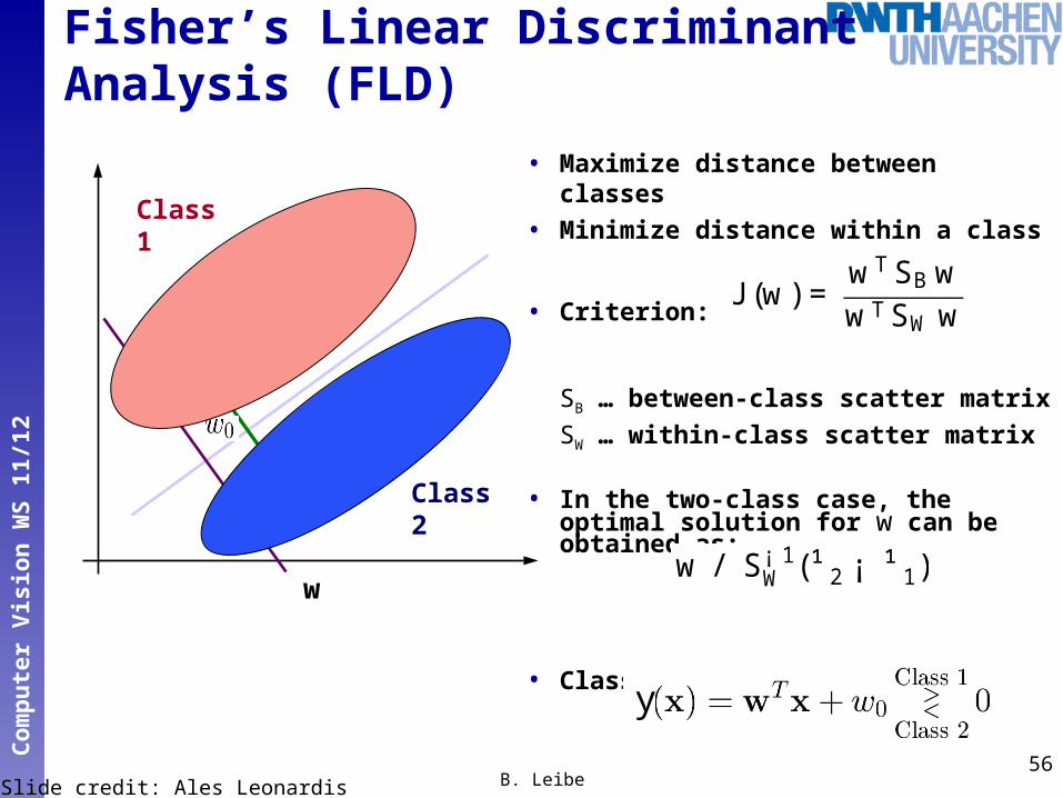
Fisher’s Linear Discriminant Analysis (FLD)
• Maximize distance between classes
• Minimize distance within a class
• Criterion:
SB … between-class scatter matrixSW … within-class scatter matrix
• In the two-class case, the optimal solution for w can be obtained as:
• Classification function:
56B. Leibe
Class 1
Class 2
w
x
x
Slide credit: Ales Leonardis
y
J (w) =wT SB wwT SW w
w / S¡ 1W (¹ 2 ¡ ¹ 1)

Perc
ep
tual an
d S
en
sory
Au
gm
en
ted
Com
pu
tin
gC
om
pu
ter
Vis
ion
WS
11
/12
Multiple Discriminant Analysis
• Generalization to K classes
where
57B. Leibe
J (W ) =jW T SB W jjW T SW W j
W = [w1; : : :;wK ]
SB =KX
k=1
Nk(¹ k ¡ ¹ )(¹ k ¡ ¹ )T
SW =KX
k=1
X
n2Ck
(xn ¡ ¹ k)(xn ¡ ¹ k)T
¹ =1N
NX
n=1
xn =1N
KX
k=1
Nk¹ k
Does this look familiarto anybody?

Perc
ep
tual an
d S
en
sory
Au
gm
en
ted
Com
pu
tin
gC
om
pu
ter
Vis
ion
WS
11
/12
Multiple Discriminant Analysis
• Generalization to K classes
where
58B. Leibe
J (W ) =jW T SB W jjW T SW W j
W = [w1; : : :;wK ]
SB =KX
k=1
Nk(¹ k ¡ ¹ )(¹ k ¡ ¹ )T
SW =KX
k=1
X
n2Ck
(xn ¡ ¹ k)(xn ¡ ¹ k)T
Does this look familiarto anybody?
Again a Rayleighquotient…
N Cut(A;B) =yT (D ¡ W )y
yT Dy

Perc
ep
tual an
d S
en
sory
Au
gm
en
ted
Com
pu
tin
gC
om
pu
ter
Vis
ion
WS
11
/12
Maximizing J(W)
• Solution from generalized eigenvalue problem
The columns of the optimal W are the eigenvectors correspon-ding to the largest eigenvectors of
Defining , we get
which is a regular eigenvalue problem. Solve to get eigenvectors of v, then from that of w.
• For the K-class case we obtain (at most) K-1 projections.
(i.e. eigenvectors corresponding to non-zero eigenvalues.)59
B. Leibe
J (W ) =jW T SB W jjW T SW W j
SB wi = ¸ i SW wi
v = S12B w
S12B S¡ 1
W S12B v = ¸v

Perc
ep
tual an
d S
en
sory
Au
gm
en
ted
Com
pu
tin
gC
om
pu
ter
Vis
ion
WS
11
/12
Face Recognition Difficulty: Lighting
• The same person with the same facial expression, and seen from the same viewpoint, can appear dramatically different when light sources illuminate the face from different directions.

Perc
ep
tual an
d S
en
sory
Au
gm
en
ted
Com
pu
tin
gC
om
pu
ter
Vis
ion
WS
11
/12
Application: Fisherfaces
• Idea: Using Fisher’s linear discriminant to find class-
specific linear projections that compensate for lighting/facial expression.
• Singularity problem The within-class scatter is always singular for face
recognition, since #training images << #pixels
This problem is overcome by applying PCA first
61B. LeibeSlide credit: Peter Belhumeur [Belhumeur et.al. 1997]
WTopt = WT
° dUTpca
Upca = argmaxU
jUT ST Uj;
W° d = argmaxW
jWT UTpcaSB UpcaWj
jWT UTpcaSW UpcaWj
ST = SB + SW

Perc
ep
tual an
d S
en
sory
Au
gm
en
ted
Com
pu
tin
gC
om
pu
ter
Vis
ion
WS
11
/12
Fisherfaces: Experiments
• Variation in lighting
62B. LeibeSlide credit: Peter Belhumeur [Belhumeur et.al. 1997]

Perc
ep
tual an
d S
en
sory
Au
gm
en
ted
Com
pu
tin
gC
om
pu
ter
Vis
ion
WS
11
/12
Fisherfaces: Experiments
Slide credit: Peter Belhumeur [Belhumeur et.al. 1997]

Perc
ep
tual an
d S
en
sory
Au
gm
en
ted
Com
pu
tin
gC
om
pu
ter
Vis
ion
WS
11
/12
Fisherfaces: Experimental Results
64B. LeibeSlide credit: Peter Belhumeur [Belhumeur et.al. 1997]

Perc
ep
tual an
d S
en
sory
Au
gm
en
ted
Com
pu
tin
gC
om
pu
ter
Vis
ion
WS
11
/12
Fisherfaces: Experiments
• Variation in facial expression, eye wear, lighting
65B. Leibe [Belhumeur et.al. 1997]Slide credit: Peter Belhumeur

Perc
ep
tual an
d S
en
sory
Au
gm
en
ted
Com
pu
tin
gC
om
pu
ter
Vis
ion
WS
11
/12
Fisherfaces: Experimental Results
66B. Leibe [Belhumeur et.al. 1997]Slide credit: Peter Belhumeur

Perc
ep
tual an
d S
en
sory
Au
gm
en
ted
Com
pu
tin
gC
om
pu
ter
Vis
ion
WS
11
/12
Example Application: Fisherfaces
• Visual discrimination task Training data:
Test:
67B. Leibe
C2: Subjects without glassesC1: Subjects with glasses
glasses?
=
Take each image as a vectorof pixel values and apply FLD…
Image source: Yale Face Database

Perc
ep
tual an
d S
en
sory
Au
gm
en
ted
Com
pu
tin
gC
om
pu
ter
Vis
ion
WS
11
/12
Fisherfaces: Interpretability
• Example Fisherface for recognition “Glasses/NoGlasses“
68B. Leibe [Belhumeur et.al. 1997]Slide credit: Peter Belhumeur

Perc
ep
tual an
d S
en
sory
Au
gm
en
ted
Com
pu
tin
gC
om
pu
ter
Vis
ion
WS
11
/12
References and Further Reading
• Background information on PCA/FLD can be found in Chapter 22.3 of
D. Forsyth, J. Ponce,Computer Vision – A Modern Approach.Prentice Hall, 2003
• Important Papers (available on webpage) M. Turk, A. Pentland
Eigenfaces for RecognitionJ. Cognitive Neuroscience, Vol. 3(1), 1991.
P.N. Belhumeur, J.P. Hespanha, D.J. KriegmanEigenfaces vs. Fisherfaces: Recognition Using Class Specific Linear Projection, IEEE Trans. PAMI, Vol. 19(7), 1997.