Percolation and conductivity of random two-dimensional composites

This article has been downloaded from IOPscience. Please scroll down to see the full text article.

1981 J. Phys. C: Solid State Phys. 14 2361

(http://iopscience.iop.org/0022-3719/14/17/009)

Download details:

IP Address: 138.67.11.96

The article was downloaded on 18/08/2011 at 19:27

Please note that terms and conditions apply.

View the table of contents for this issue, or go to the journal homepage for more

Home Search Collections Journals About Contact us My IOPscience

J. Phys. C : Solid State Phys., 14 (1981) 2361-2376. Printed in Great Britain

Percolation and conductivity of random two- dimensional composites

P H Winterfeld, L E Scriven and H T Davis Departments of Chemical Engineering and Materials Science and of Chemistry, University of Minnesota, Minneapolis, MN 55455, USA

Received 15 August 1980, in final form 22 December 1980

Abstract. Tessellatingan areainto convex polygons andlabelling a given number ofrandomly chosenpolygons as conducting, the rest not, creates ausefulmodelof adisorderedcomposite. The percolation and conduction properties of composites generated from the random Voronoi tessellation are compared with those from regular tessellations, namely the square and the hexagonal. Percolation properties of interest are the conducting cluster distribution, the percolation threshold, and the percolation probability. Conduction properties are obtained by a lattice network reduction (a finite difference type approximation to conduc- tion) and by finite element analysis. TWO finite element analyses arise, one from imposing a potential drop across the system and another from imposing a current flow through it; the two yield upper and lower bounds, respectively, to the true conductivity. By refinement of the finite element technique, convergence of the bounds is obtained. The percolation thresholds and percolation probabilities of the Voronoi and hexagonal tessellations are indistinguishable, a reflection presumably of the fact that both tessellations are equivalent to a fully triangulated two-dimensional lattice. The average coordination number (number of edges of a polygon) of the Voronoi and hexagonal tessellations are identical. Their cluster distributions are similar although those of the Voronoi tessellation are slightly broader. Percolation properties as well as conduction properties of the square tessellation differ markedly from the others. Finite element analysis shows that the conductivity of the hexag- onal composite lies above that of the Voronoi composite, indicating an increased resistance to transport caused by the random geometry of the Voronoi tessellation. The lattice network reduction yields the right qualitative features of the conductivity but not very accurate values.

1. Introduction

The relationship between percolation theory and conduction in disordered systems has been firmly established (Ziman 1968, Eggarter and Cohen 1970,1971, Kirkpatrick 1971, 1973, Last and Thouless 1971, Stinchcombe 1973, 1974). The present state of the understanding of such systems is based primarily on either idealised network models or effective medium theory (Kirkpatrick, 1973, Stinchcombe 1973,1974, Bruggeman 1935, Landauer 1952, Cohen and Jortner 1973). Neither of these is entirely satisfactory for describing conduction in continuous media. Effective medium theory is a statistical model which averages over the actual structure of the system and consequently cannot account for the conductivity behaviour of systems near the percolation threshold. Through a suitably defined finite difference approximation, the conduction problem of

0022-3719/81/172361 -!- 16 $01.50 @ 1981 The Institute of Physics 2361

2362 P H Winterfeld, I, E Scriven and H T Davis

a continuous medium can be reduced to a lattice network problem. The percolation behaviour of such a lattice reduction depends, however, on the nature of the tessellation used, which is usually square (2D) or cubic (3D) cells, to subdivide the volume of the system to discretise the continuum problem. Moreover, the finite difference solution generally does not provide either an upper or a lower bound to the average or effective conductivity of the medium.

The purpose of this paper is to investigate the effect of the tessellation on the percolation behaviour of a disordered composite medium and to compare the conduc- tivity of network reductions with that predicted by more rigorous numerical analysis of the conduction problem.

A novel technique of modelling a two-dimensional composite, easily extendable to three dimensions, is presented here. Area is subdivided into random polygons by what is known as the Voronoi (1908) tessellation. A random, two-component composite is generated by labelling a given fraction of randomly selected polygons as one material and the remaining polygons as another material. For the present studies one material will be considered conducting and the other insulating. Percolation properties of the composite, such as the percolation threshold, cluster distribution. and percolation probability are generated by computer simulation. The conductivity of the continuous medium is found by finite element methods (Fix and Strang 1973) yielding lower and upper bounds on the conductivity. The results for the Voronoi tessellation are compared with those of square and hexagonal tessellations and of corresponding netwcrk reduc- tions. Random networks derived from Voronoi tessellated composites have been studied previously by Hatfield (1978).

2. The Voronoi tessellation

The Voronoi tessellation, or Meijering’s (1953) cell model, is a method for subdividing a continuum into random, convex polytopes, i.e. polyhedra in three dimensions and polygons in two. The tessellation is made by distributing points (‘Poisson’ points) randomly in space, and for each point, bisecting each segment joining it and every other Poisson point with a line (2D) or plane (3D) orthogonal to the line between the points, and constructing the minimum polytope about the point formed by the intersection of the bisecting planes. A two-dimensional example is shown in figure 1.

A network representation of the Voronoi tessellation can be cons1 ructed by rep- resenting each polygon as a site, located for convenience at its Poiswm point, and inserting bonds connecting the sites of neighbouring polygons. The coordination number z of a site in the network is equal to the number of edges of the polygon associated with the site. Similar networks can be constructed for square or regular hexagon tessellations. The percolation properties of a tessellated continuum are the same as those of the corresponding network under conditions of site percolation.

Hatfield (1978) investigated the percolation properties of random networks gener- ated from Voronoi polygons. The three-dimensional tessellation was used by Finney (1970) to model random-sphere packs and by Prager and Talmon (1077) to model oil- water-surfactant microemulsions.

A conductor-insulator composite is created by randomly selecting a number of polytopes to be conducting and the rest insulating. Figure 2 shows two-dimensional examples. In figure 2(a) the area fraction covered by conducting polygons is so small that there are no sample spanning (percolating) clusters; hence that sample is below its

Random two-dimensional composites 2363

Figure 1. Voronoi tessellation with 160 polygons. Dots indicate randomly located Poisson points

Ibl Figure 2. (a ) Composite with low area fraction conducting polygons. ( b ) Composite with high area fraction conducting polygons.

2364 P H Winterfeld, L E Scriven and H T Davis

percolation threshold (strictly speaking the percolation threshold is only defined for an infinitely large sample) and would not conduct if a potential were imposed across it. Figure 2(b) shows a composite having an area fraction of conducting material sufficiently high that the sample would conduct if a potential were imposed.

3. Percolation properties

The percolation properties sought here can be defined by imagining random removal of conducting polygons (sites) from an infinitely large tessellation (network) of conductors. In the tessellation, a cluster is defined as an isolated, finite group of conducting polygons in electrical contact with one another. Correspondingly, in a network a cluster is a group of sites connected by conducting bonds. If enough polygons (sites) are removed that the fraction w of conducting polygons (sites) is below the percolation threshold wc, then the conducting paths exist only in the clusters and the system behaves as an insulator. If the polygon fraction w is above the percolation threshold, an infinite cluster exists, implying for any finite system the existence of a continuous conducting path across the system. The fraction P(w) of conducting polygons involved in the infinite or sample-spanning cluster is known as the percolation probability and in large but finite samples has been called the accessible fraction (Larson et al1981) to emphasise that the polygons making up P(w) allow conduction between opposed edges of the system. For w > U, the system conducts under an externally applied potential and for w < o, it does not,

The lattice representation of an infinite two-dimensional Voronoi tessellation is a fully triangulated lattice, defined as an infinite multiply connected planar graph all of whose finite faces are triangular. Sykes and Essam (1964) have argued that fully trian- gulated lattices are self matching and consequently have a percolation threshold of 4; exceptions do exist however (Van den Berg 1981). We have determined by computer simulation the percolation thresholds, the coordination number distribution and the cluster distribution. The data presented here for these quantities were determined from the average of ten different Voronoi tessellations, each containing 10000 polygons. Uncertainties are expressed as one-sample standard deviation.

The percolation threshold of the Voronoi tessellation, computed from the cluster moment method of Dean (1963), is

w, = 0.500 k 0.010.

From the conducting fraction at which a sample-spanning chain first forms, we obtained the similar estimate, wc = 0.502 t 0.016. For square and hexagonal tessellations, the percolation thresholds are 0.591 and 0.500 respectively (Dean and Bird 1966). The lattice representation of the hexagonal tessellation is also a fully triangulated lattice.

The coordination number distribution @ ( z ) for the Voronoi tessellation is given in table 1. The bias introduced by the square boundary was minimised by discarding all polygons in contact with it, reducing the number of polygons contributing to the distri- bution to approximately 9650 for each tessellation. The average coordination number, C,@(z), obtained from the distribution is 5.99 i 0.05, the difference between this number and the exact value of six being an indicator of the effect of finite sample size on the statistics of the tessellation. There are of course no polygons with z less than 3.

Let us denote by v(n, w ) the probability that a polygon exists in an n-polygon cluster in an infinite tessellation having a fraction o of conducting polygons. For a sufficiently large tessellation LL) is the area fraction of conducting polygons and u(n, w ) is the area

Random two-dimensional composites 2365

Table 1.

Z W )

3 0.01154 t 0.00095 4 0.10942 t 0.00269 5 0.26064 t 0.00483 6 0.29387 t 0.00417 7 0.19769 t 0.00404 8 0.08932 2 0.00271 9 0.02850 t 0.00136

10 0.00724 t 0.00074 11 0.00146 t 0.00045 12 0.00027 i: 0.00017 13 0.00006 t 0.00007 14 0

fraction of clusters of size n. f ( n , w), the frequency of clusters of size n, is given by

f ( n , U) = v(n, @)in. ( 2 ) In principle, v(n, 0) can be computed theoretically from the coordination number

distribution @(z) . The first three-cluster distributions for any convex tessellation are

v(1, w) = x 2 w@(z) (1 -

4 2 , 0) = 2 , x 2' zw2@(z) @ ( z ' ) (1 - U)' + 2' -

( 3 )

(4)

where the z , z' = 3 , 3 term is excluded as explained below, and

4 3 , 0) = 5: 03@(z) qz') @(Z")( l - wy + 2' + z" - g ( w , Z , Z ' > ( 5 ) 2, z , 2"

l i i l l l l l l

0.06 n = l

Conducting f ract ion w

Figure 3. Cluster distribution data for 10000 polygon Voronoi tessellations,

2366 P H Winterfeld, L E Scriven and H T Davis

0.06 I

3

L a. +

2 0 U

Conducting fraction w

Figure 4. Cluster distribution for hexagonal tessellation (from Dean arid Bird 1966).

where

g(w, z, 2‘) = gdw 2 , z’) + g2(z) + g3(4

gl(w, Z, 2’) = [z(z’ - 3 ) + ( z ’ / ~ ) ( z ’ - 3)] (1 - CO) (6a)

g2(z> = 2 (6b)

g3(w) = Q43) (1 - w2. (6c)

The constraint on z, z’ values in equation (4) arises from the condition of convexity in

Conducting fraction w

Figure 5. Cluster distribution for square tessellation (from Dean and Bird 1966).

Random two dimensional composites 2367

Figure 6. Percolation probabilities for 10000 polygon Voronoi, square, and hexagonal tessellations.

the Voronoi tessellation. Convexity also imposes the following constraints on the sum- mations of equation ( 5 ) . For gl, z' begins at 4, terms 3 , 4 , 3 and 3 , 5 , 3 are excluded; for g2 any combination of 3 ,4 , and 4 and any containing two threes are excluded; for g3, all the indices begin with 4, and all combinations containing two fours and 4,5, and 5 are excluded. For a square tessellation @ ( z ) = 1 if z = 4 and is zero otherwise; for a hexa- gonal tessellation @ ( z ) = 1 if z = 6 and is zero otherwise. The formulae for larger clusters are quite complicated and are not used here.

Figures 3, 4 and 5 give examples of the dependence of v(n, w ) on 10 for Voronoi, hexagonal, and square tessellations. The cluster distributions were computed from equations (4) and (5) for n = 1 ,2 , and 3 and from computer simulations for n > 3. The

'\ 0 r, Figure 7. Schematic of conducting domain. showing different types of boundaries.

2368 P H Winterfeld, L E Scriven and H T Davis

cluster distributions of the Voronoi and hexagonal tessellations are quite similar. How- ever, for small clusters, the Voronoi results lie noticeably above the hexagonal, a consequence of the Voronoi distribution of coordination numbers. A greater fraction of polygons have coordination number less than six than have more than six. Polygons with smaller coordination number are less likely to have conducting neighbours than those with higher coordination number. The computer-estimated percolation probabil- ities of Voronoi, hexagon, and square tessellations are compared in figure 6. At high conducting fractions, the percolation probability is equal to the conducting fraction. The data for the square drops off at a higher conducting fraction than either the Voronoi or hexagonal due to its higher percolation threshold. There is little difference between the Voronoi and the hexagonal results.

4. Effective conductivity of a conductor-insulator composite

4.1. Basic problem

For present purposes a 2D composite is generated by randomly selecting a number of polygons to be conducting, the rest being insulating. An effective conductivity is defined and computed for each tessellation and for its network reduction. The computer storage requirements and costs are considerably greater for determining the conductivity than the 'topological' percolation properties obtained in the previous section Thus, we were forced to use much smaller systems, ranging in size from 160 to 1100 polygons, for conductivity studies. For this reason, our results will be a poor approximation to the properties of large tessellations. However, the main goal is to compare tessellations and their network reductions with each other, so our conductivity results can be achieved with small systems.

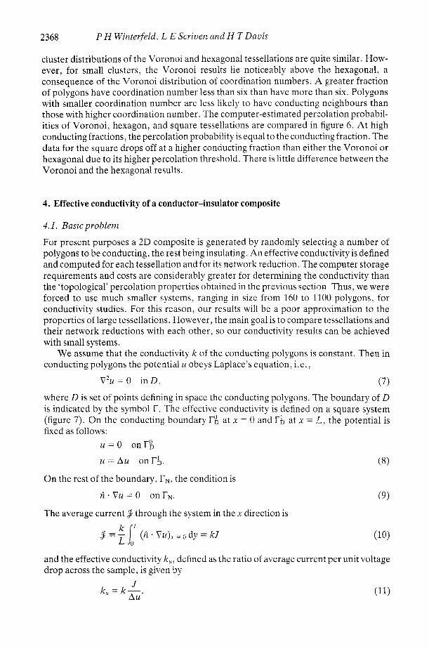
We assume that the conductivity k of the conducting polygons is constant. Then in conducting polygons the potential U obeys Laplace's equation, i.e.,

V 2 u = 0 i n D , (7) where D is set of points defining in space the conducting polygons. The boundary of D is indicated by the symbol r. The effective conductivity is defined on ii square system (figure 7). On the conducting boundary r k at x = 0 and rb at x = L, the potential is fixed as follows:

U = O o n r b

U = A u o n r b . (8)

A . V u = O o n r x . (9)

On the rest of the boundary, TN, the condition is

The average current $ through the system in the x direction is

and the effective conductivity k,,, defined as the ratio of average current per unit voltage drop across the sample, is given by

Random two-dimensional composites

A result deduced from equations (7)-(9) is

JAu = (Vu)' dx dy E I ( u ) , J and so

k , - J - Z(u) - J 2 k Au ( A u ) ~ Z(u)' - = - - - - -

2369

(12)

These formulae will enable us to compute upper and lower bounds for k,/k in a systematic way.

4.2. Resistor network approximation of conduction

A resistor approximation to conduction is obtained from the lattice representation of tessellation. Each bond of the network has a current J , and a resistance Ri associated with it such that, ideally, the conductivity of the resistor network should equal that of the actual composite. By equating the energy dissipation rate ($ALL), of each, we obtain

r

J ~ R ; = J,, k(Vu)' dA,

Ai, the area represented by bond i , is the quadrilateral obtained by connecting the vertices determining an edge to the Poisson points on either side of it. J; is arbitrarily defined as the current flowing out of a polygon face.

The resistance of bond i is

Since the potential gradient is divergenceless, the net current flow out of a polygon of z sides is zero:

In the resistor network approximation, the potential gradient field is approximated as

where A/, is the unit normal to edge i. This approximation yields the resistance

dilkli k # 0 inAi

0 k = 0 anywhere in A i

where di is the length of bond i and li is the length of edge i. The C,'s are evaluated by minimising the energy dissipation of the resistor network with equation (17) as a con- straint. This gives

2310 P H Winterfeld, L E Scriven and H T Davis

or

V,, a constant associated with site a, can be interpreted as a nodal potential. It is determined by equations (21), (17) and the boundary conditions given by equations (8) and (9).

The conductivity of the resistor network is defined analogously to that of the actual composite:

Conducting fraction w

Figure 8. Effective conductivity data for 160 polygon Voronoi tessellation-resistor network approximation.

where Jbn, is the current flowing through a bond connected to the boundaryr;. Potential drop, current flow, and energy dissipation are related analogously to equation (12):

J T A U = I J?Ri. (23)

Equation (23) becomes

analogous to equation (13). Computer simulations of the resistor network model have been made for ten Voronoi

tessellations each containing 160 polygons. Averages of the ten trials, with bars rep- resenting one-sample standard deviation, are shown in figure 8. This format for computer simulations is used throughout the rest of this paper.

Random two-dimensional composites 237 1

4.3. Finite element computations The resistor network is only a qualitatively correct approximation to Laplace’s equation. Accurate approximations to it can be obtained by the finite-element Galerkin method.

The conducting domain D is subdivided into triangular elements by connecting the Poisson point (or the centre for squares and hexagons) of each conducting polygon to the vertices of the polygon. The mesh can be refined by connecting the midpoints of the sides of each triangular element, thereby creating four congruent triangular elements from each one in the original subdivision. The mesh can be further refined by repeating the procedure. The variational formulation of equations (7)-(9) is:

I( U ) 3 I( U) (25) where U is contained inHk, the set of all functions which satisfy the essential boundary condition (equation (8)) and, along with their first derivatives, are square integrable in the sense of Lebesgue. Using the Ritz approximation, a trial solution uN contained in a subspace of HL spanned by Nlinearly independent, piecewise linear, finite element basis functions is expressed as

qi, the weighting factor of vi, the basis function, is determined by minimising I( u N ) . The conductivity of this finite element approximation is defined as

From equation (25), k J k is an upper bound to k,lk. Equation (25) is the Dirichlet principle for the conduction problem. It has a dual

principle called the Kelvin principle (Serrin 1959), which leads to a lower bound rather than an upper one. The Kelvin principle is built on the current vector j which must be solenoidal because there are no current sources within the conductor:

V . j = 0 (28)

V X j = O . (29)

j = V X A . (30)

The current vector must be the gradient of a potential so its curl must vanish:

Since j is solenoidal, it can be written as the curl of a vector potential

In two dimensions, A can be expressed in terms of a scalar current function,

A = kA(X, Y).

Then

V X V X A = V 2 A = 0 i n D (32) where

A = constant on rN (33)

n VA = 0 onTD. (34)

2372 P H Winterfeld, L E Scriven and H T Davis

Equations (33) and (34) are equivalent boundary conditions to equations (8) and (9) respectively. This current function, or stream function, formulation has a variational formulation that is conjugate to that of the potential formulation (Aubin 1972).

Z(A) 2 Z(A) = Z(u) (35) where A is contained in Hh, the essential boundary condition being equation (33).

The total current flow per unit cross section calculated from equation (10) becomes:

the overall difference of current function across a conducting face. Imposing equation (36) only determines A on part of r N . A is determined on the rest of IyK by setting I(A) to equal to Z(u).

Finite element approximations for A are obtained on the same meshes and use the same basis functions as those for U. On those regions of r N where A is constant yet not determined as a result of imposing total current flow, constant A is imposed on each interval by superposing the basis functions of the nodes there into sets of ‘extended’ basis functions having one weighting factor each; the value of A on that portion of the boundary.

The conductivity of this finite element approximation is given by:

From equation (25), kA/k is a lower bound to k,!k. Figure 9 shows the results of computer simulations calculating coarse and refined

Figure 9. Effective conductivity data for 160 polygon Voronoi tessellations-finite element approximations--upper and lower bounds on coarse and refined meshes.

Random two-dimensional composites 2373

Conducting fraction w Conducting fraction w

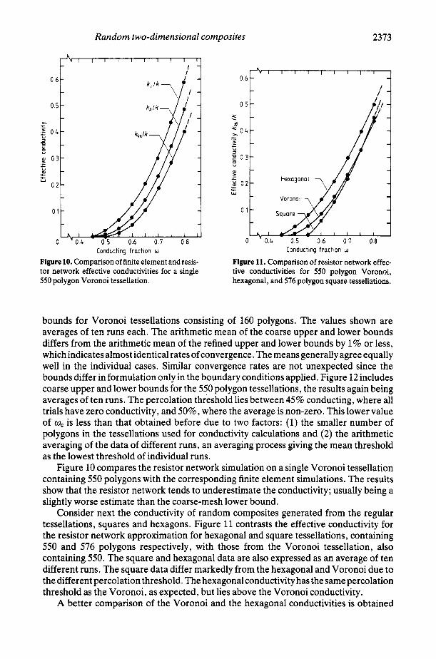
Figure 10. Comparison of finite element and resis- tor network effective conductivities for a single 550 polygon Voronoi tessellation.

Figure 11. Comparison of resistor network effec- tive conductivities for 550 polygon Voronoi, hexagonal, and 576 polygon square tessellations.

bounds for Voronoi tessellations consisting of 160 polygons. The values shown are averages of ten runs each. The arithmetic mean of the coarse upper and lower bounds differs from the arithmetic mean of the refined upper and lower bounds by 1% or less, which indicates almost identical rates of convergence. The means generally agree equally well in the individual cases. Similar convergence rates are not unexpected since the bounds differ in formulation only in the boundary conditions applied. Figure 12 includes coarse upper and lower bounds for the 550 polygon tessellations, the results again being averages of ten runs. The percolation threshold lies between 45% conducting, where all trials have zero conductivity, and 50%, where the average is non-zero. This lower value of w, is less than that obtained before due to two factors: (1) the smaller number of polygons in the tessellations used for conductivity calculations and (2) the arithmetic averaging of the data of different runs, an averaging process giving the mean threshold as the lowest threshold of individual runs.

Figure 10 compares the resistor network simulation on a single Voronoi tessellation containing 550 polygons with the corresponding finite element simulations. The results show that the resistor network tends to underestimate the conductivity; usually being a slightly worse estimate than the coarse-mesh lower bound.

Consider next the conductivity of random composites generated from the regular tessellations, squares and hexagons. Figure 11 contrasts the effective conductivity for the resistor network approximation for hexagonal and square tessellations, containing 550 and 576 polygons respectively, with those from the Voronoi tessellation, also containing 550. The square and hexagonal data are also expressed as an average of ten different runs. The square data differ markedly from the hexagonal and Voronoi due to the different percolation threshold. The hexagonalconductivity has the same percolation threshold as the Voronoi, as expected, but lies above the Voronoi conductivity.

A better comparison of the Voronoi and the hexagonal conductivities is obtained

2374 P H Winterfeld, L E Scriven and H T Davis

Conducting fraction w

Figure 12. Comparison of finite element upper and lower coarse mesh bounds for effective conductivity of 550 polygon Voronoi and hexagonal tessellations. Stippled area indicates overlap of Voronoi and hexagonal bounds.

from finite element simulations. Figure 12 contrasts the upper and lower bounds for the conductivities of the same Voronoi and hexagonal tessellations represented in figure 11. The upper Voronoi bound and the lower hexagonal roughly coincide; the regions between the bounds do not overlap significantly. Dotted lines midway between the bounds indicate approximately where the exact solution lies. The lower Voronoi con- ductivity results from its more random structure: a given conducting path has many constrictions, from short edges, that impede current flow, lowering the conductivity.

Conducting fraction w

Figure 13. Approximation of effective conductivity of infinite Voronoi tessellation.

Random two-dimensional composites 2375

No such effect exists in the uniform hexagonal medium. Also, the hexagonal bounds are much closer together than are the Voronoi's: the finite element mesh in the hexagonal is uniform, compared with the random mesh in the Voronoi. This results in a better approximation to the conductivity.

An estimate of an infinite Voronoi tessellation has been obtained by plotting the conductivity data for 550 and 1100 polygon tessellations versus the inverse of the tessellation size and extrapolating to zero-an infinite tessellation. The mean of the extrapolated bounds, the estimate for the infinite system, is shown in figure 13. Above 60% of conducting polygons, little difference exists between the conductivity of the systems having 550,1100, and (extrapolated) infinite polygons. Below 60% the conduc- tivity becomes increasingly more sensitive to sample size as the percolation threshold is approached.

5. Summary

The percolation and conduction properties of random composites depend on the coor- dination number and geometry of the tessellation. The percolation threshold and per- colation probability depend on the average coordination number of the tessellation: identical results for these were obtained for the Voronoi and hexagonal tessellations both with average coordination number of six. Their cluster distributions were similar. The differences evident at higher conducting fractions were due to the random distri- bution of coordination number in the Voronoi. Percolation properties of the square tessellation differed markedly from the others,

Conduction simulations on random composites generated from these tessellations further reflected these trends. Resistor network simulations revealed a discrepancy between the square's conductivitjl and the others as expected from the percolation threshold data. Finite element analysis showed that the conductivity of the hexagonal composite lies above that of the Voronoi composite, a trend accountable for by the random geometry of the Voronoi tessellation.

References

Aubin J P 1972 Approximation to Elliptic Boundary Vulue Problems (New York: Wiley) Broadbent S R and Hammersley J M 1957 Proc. Camb. Phil. Soc. 53 629-41 Bruggemann D A G 1935 A n n . Phys., Lpz . 24 636-79 Cohen M H and Jortner 1973 Phys. Rev. Lett. 30 699--702 Dean P 1963 Proc. Camb. Phil. Soc. 59 397-410 Dean P and Bird N F 1966 Ma 61 National Physics Laboratory. Mathematics Div. Eggarter T P and Cohen M H 1970 Phys. Rev. Lett. 25 807-10 - 1971 Phys. Rev. Lett. 27 129-32 Finney J L 1970 Proc. R . Soc. A 319 479-93 Hammersley J M 1957 Proc. Camb. Phil. Soc. 53 642-5 Hatfield J C 1978 PhD Thesis University of Minnesota Kirkpatrick S 1971 Phys. Rev. Lett. 27 1722-5

Landauer R 1952 J . Appl . Phyx 23 779-84 Larson R G, Scriven L E and Davis H T 1981 Chem. Eng. Sci. 36 57-73 Last B J and Thouless D J 1971 Phys. Rev. Lett. 27 1719-21 Meijering J L 1953 Philips Res. Rep. 8 27&90 Prager S and Talmon Y- 1977 Nature 267 333-5

- 1973 Rev. Mod. Phys. 45 574-88

2376 P H Winterfeld, L E Scriven and H T Davis

Serrin J 1959 Mathematical Principles of Classical Fluid Mechanics in Encyclopedia o f Physics vol 18, no 1,

Stinchcombe R B 1973 J . Phys. C: Solid State Phys. 6 L1-5 - 1974 J. Phys. C: Solid State Phys. I 179-203 Strang G and Fix G J 1973 An Analysis of the Finite Element Method (Englewood Cliffs, NJ: Prentice-Hall) Sykes M F and Essam J W 1964 J . Math. Phys. 5 1117 Van den Berg J 1981 J . Math. Phys. 22 152-61 Voronoi G 1908 J . reine angew. Math. 134 198-287 Ziman J M 1968 J . Phys. C: Solid State Phys. 1 1532-8

pp 125-30