inference and experimental design for percolation and random graph models
TRANSCRIPT

Inference and Experimental Design for
Percolation and Random Graph Models
Andrei Iu. Bejan, PhD, MSc
Submitted for the degree of
Doctor of Philosophy
on completion of research in the
Department of Actuarial Mathematics and Statistics,
School of Mathematical and Computer Sciences,
Heriot-Watt University
June 2010
The copyright in this thesis is owned by the author. Any quotation from the thesis
or use of any of the information contained in it must acknowledge this thesis as
the source of the quotation or information.

Abstract
The problem of optimal arrangement of nodes of a random weighted graph is
studied in this thesis. The nodes of graphs under study are fixed, but their edges
are random and established according to the so called edge-probability function.
This function is assumed to depend on the weights attributed to the pairs of graph
nodes (or distances between them) and a statistical parameter. It is the purpose
of experimentation to make inference on the statistical parameter and thus to
extract as much information about it as possible. We also distinguish between two
different experimentation scenarios: progressive and instructive designs.
We adopt a utility-based Bayesian framework to tackle the optimal design
problem for random graphs of this kind. Simulation based optimisation meth-
ods, mainly Monte Carlo and Markov Chain Monte Carlo, are used to obtain
the solution. We study optimal design problem for the inference based on partial
observations of random graphs by employing data augmentation technique.
We prove that the infinitely growing or diminishing node configurations asymp-
totically represent the worst node arrangements. We also obtain the exact solution
to the optimal design problem for proximity graphs (geometric graphs) and numer-
ical solution for graphs with threshold edge-probability functions.
We consider inference and optimal design problems for finite clusters from bond
percolation on the integer lattice Zd and derive a range of both numerical and
analytical results for these graphs. We introduce inner-outer plots by deleting
some of the lattice nodes and show that the ‘mostly populated’ designs are not
necessarily optimal in the case of incomplete observations under both progressive
and instructive design scenarios.
Finally, we formulate a problem of approximating finite point sets with lattice
nodes and describe a solution to this problem.
i

To my grandparents.
ii

Statement of Authorship
Some parts of this thesis have been published or submitted for publication in
refereed journals, presented at conferences and used in teaching materials. Listed
below is the information pertaining to these preliminary presentations of results.
1. Bejan, A. Iu. (2009) Inference and optimal design for percolation and random
graph models. Computer Laboratory Opera Group Seminars. The University
of Cambridge.
2. Bejan, A. Iu. (2009) Large clusters as rare events, their simulation and con-
nection to critical percolation. Networks (Operations Research) Seminar
Series. The University of Cambridge.
3. Bejan, A. Iu. (2008) Grid approximation of a finite set of points. Conference
Mathematics & IT: Research and Education 2008, Chişinău, October 1-4.
4. Bejan, A. Iu., Gibson, G. J., Zachary, S. (2008) Inference and experimental
design for some random graph models. Workshop Designed Experiments:
Recent Advances in Methods and Applications (DEMA2008), Isaac Newton
Institute for Mathematical Sciences, Cambridge, UK, 11-15 August 2008.
5. Bejan, A. (2008) Lecture notes “MCMC in modern applied mathematics”.
Center for Education and Research in Mathematics and Computer Science,
Department of Mathematics and Computer Science, State University of Moldova.
http://www.cl.cam.ac.uk/~aib29/CECMI/MCMC/notes.pdf
6. Cook, A. R., Gibson, G. J., Gilligan, C. A. (2008) Optimal observation times
in experimental epidemic processes. Biometrics, 64(3), pp. 860-868.
iii

with Web Appendices at
http://www.biometrics.tibs.org/datasets/070104.pdf
Except where explicit reference is made in the text of the thesis, this thesis
contains no material published elsewhere or extracted in whole or in part from a
thesis by which I have qualified for or been awarded another degree or diploma. No
other person’s work has been relied upon or used without due acknowledgement
in the main text and bibliography of the thesis.
iv

Acknowledgements
I was suggested to undertake this study by Professor Gavin Gibson in reply to my
proposal for pursuing PhD research at Heriot–Watt University in 2005. Gavin’s
suggestion was to consider an abstract problem of identifying spatial locations
of nodes of a random graph that make observation of the edge structure most
informative about the statistical model underlying the formation of the graph and
to look at the applications, particularly in plant epidemiology, where observations
often tend to be a filtering of the above graph. Dr Stan Zachary, Heriot–Watt
University, joined the supervising team with interests and expertise in probability
theory and stochastic network analysis.
I would like to express my sincere gratitude in the first place to my supervisors
for the enormous amount of time and support they have given to me. I would also
like to thank my examiners, Professor Frank Ball, The University of Nottingham,
and Dr George Streftaris, Heriot-Watt University for useful comments and critical
observations which undoubtedly resulted in the improvement of the thesis.
I thank Professor Chris Gilligan, The University of Cambridge, for his hospi-
tality in February 2007 and for permission to reproduce Figure 1.3 from Bailey,
Otten and Gilligan (2000).
I thank Dr. Alex Cook (Heriot-Watt University, University of Cambridge, Na-
tional University of Singapore) for permanent discussions on the topic and also for
the plants he was so generous to give me. The plants are in good health and I can
say that many people enjoy them!
My thanks and appreciation are also extended to the following people who have
supported me in undertaking this research programme: Dr. Arkadii Semenţul,
State University of Moldova, and Professor Gheorghe Mişcoi, Academy of Sciences
v

of Moldova.
These people made my social life in Scotland enjoyable: John Phillips, Michael
Reidman, Jafar Fazilov, Wenny Chen, Eyad Al’Okke, Cornelius Schmidt-Colinet
and Ben Hart. Edinburgh is a truly great city and can hardly be compared to any
other city in the world! I thank all its tourists, especially those who leave the city
at the end of August each year, letting it get back to normal life!
Perhaps one should agree with William Somerset Maugham, who said that
“Money is like a sixth sense without which you cannot make a complete use of
the other five”. PhD students need this sixth sense indeed to fully concentrate on
their studies. The Overseas Research Student Awards Scheme (ORSAS) and James
Watt scholarship provided me with financial help and I acknowledge this support.
The British Government should be thanked for running the former, whereas the
School of Mathematical and Computer Sciences of Heriot–Watt University should
be thanked for providing me with the latter.
I am thankful to the organisers of the workshop Design of Experiments 2008
and to the Isaac Newton Institute for Mathematical Sciences for their hospitality
while attending the event. I am also thankful to EURANDOM (European Institute
for Statistics, Probability, Stochastic Operations Research and its Applications)
for organising the series of workshops Young European Probabilists, two of which
I had the chance to attend.
Finally, I am deeply indebted to my family. I owe my persistence to my grand-
parents, Ivan Nikolaevich Bejan and Ol’ga Leont’evna Bodnar’. My parents, Li-
ubov’ and Yurii, and my brother, Serguei, should be thanked for their encouraging
understanding and support. My wife, Kitty, deserves thanks for tolerating the
combination of almost incompatible things—scientific research and family life.
Andrei Bejan
Cambridge, May 2010
vi

This page is so the Research Thesis Submission Form can have the page number
before the Contents page number.
vii

Contents
Abstract i
Authorship iii
Acknowledgements v
1 Introduction 1
1.1 Why inference and optimal design on random graphs? . . . . . . . . 1
1.2 General model description and further motivation . . . . . . . . . . 4
1.2.1 Model . . . . . . . . . . . . . . . . . . . . . . . . . . . . . . 4
1.2.2 Motivation: theoretical positions and practical aspects . . . 6
1.3 Related work on inference and experimental design problems for
stochastic interaction and spatial response models . . . . . . . . . . 11
1.3.1 Spatial response models . . . . . . . . . . . . . . . . . . . . 12
1.3.2 Stochastic interaction models . . . . . . . . . . . . . . . . . 13
1.4 Outline of the thesis . . . . . . . . . . . . . . . . . . . . . . . . . . 14
2 Tools and methodology 16
2.1 Basic notions from the graph theory . . . . . . . . . . . . . . . . . . 16
2.2 Likelihood and Bayesian statistical inference . . . . . . . . . . . . . 22
2.2.1 Data, likelihood and Fisher information . . . . . . . . . . . . 23
2.2.2 Bayesian concept . . . . . . . . . . . . . . . . . . . . . . . . 27
2.3 Monte Carlo methods and Markov Chain Monte Carlo . . . . . . . 31
2.3.1 Monte Carlo methods . . . . . . . . . . . . . . . . . . . . . . 31
2.3.2 Markov Chain Monte Carlo . . . . . . . . . . . . . . . . . . 33
viii

3 Utility-Based Optimal Designs within the Bayesian Framework 41
3.1 Introduction: from locally D-optimum to utility-based Bayesian de-
signs . . . . . . . . . . . . . . . . . . . . . . . . . . . . . . . . . . . 41
3.1.1 Toy examples: three and four nodes . . . . . . . . . . . . . . 41
3.1.2 Utility-based Bayesian optimal designs . . . . . . . . . . . . 47
3.2 Shannon entropy, Lindley information measure and Kullback–Leibler
divergence . . . . . . . . . . . . . . . . . . . . . . . . . . . . . . . . 49
3.2.1 Bits of history . . . . . . . . . . . . . . . . . . . . . . . . . . 49
3.2.2 Lindley information . . . . . . . . . . . . . . . . . . . . . . . 51
3.2.3 Comparing informativeness of experiments: expected Kullback–
Leibler divergence and expected Lindley information gain as
expected utility and their properties . . . . . . . . . . . . . . 53
3.3 Progressive and Instructive Designs . . . . . . . . . . . . . . . . . . 60
3.3.1 Progressive designs . . . . . . . . . . . . . . . . . . . . . . . 61
3.3.2 Instructive designs . . . . . . . . . . . . . . . . . . . . . . . 62
3.4 Simulation-based evaluation of the expected utility . . . . . . . . . 62
3.5 Second formulation of the problem . . . . . . . . . . . . . . . . . . 65
3.5.1 The model . . . . . . . . . . . . . . . . . . . . . . . . . . . . 65
3.5.2 n-node optimal design problem for random graphs . . . . . . 66
3.5.3 Examples . . . . . . . . . . . . . . . . . . . . . . . . . . . . 67
4 Optimal Designs for Basic Random Graph Models 70
4.1 Worst case scenarios: indefinitely growing or diminishing vertex
configurations . . . . . . . . . . . . . . . . . . . . . . . . . . . . . . 70
4.2 Optimal designs for basic random graphs . . . . . . . . . . . . . . . 73
4.2.1 Two-node design and prior entropy asymptote of the ex-
pected utility . . . . . . . . . . . . . . . . . . . . . . . . . . 73
4.2.2 Progressive and instructive designs: two-node ‘black box’
design example . . . . . . . . . . . . . . . . . . . . . . . . . 76
4.2.3 Three-node star design with two independent edges . . . . . 80
4.2.4 Proximity graphs . . . . . . . . . . . . . . . . . . . . . . . . 83
4.2.5 Step-like (threshold) probability decay . . . . . . . . . . . . 88
ix

4.2.6 Non-preservation of optimal designs under replication . . . . 91
5 Lattice-based Optimal Designs 95
5.1 Inference and Optimal Design for Percolation Models . . . . . . . . 96
5.1.1 Nearest-neighbour interaction model and percolation . . . . 96
5.1.2 Parameter estimation . . . . . . . . . . . . . . . . . . . . . . 101
5.1.3 Bayesian optimal designs and inner-outer plots . . . . . . . . 120
5.1.4 Implementation of progressive and instructive designs based
on inner-outer plots . . . . . . . . . . . . . . . . . . . . . . . 129
5.2 Lattice designs for inference on random graphs with long-range con-
nections . . . . . . . . . . . . . . . . . . . . . . . . . . . . . . . . . 133
5.2.1 Generalising results from the previous section . . . . . . . . 134
5.2.2 Square lattice and its deformations . . . . . . . . . . . . . . 135
6 Grid Approximation of a Finite Set of Points 142
6.1 Formulation of the problem . . . . . . . . . . . . . . . . . . . . . . 142
6.1.1 Basic examples . . . . . . . . . . . . . . . . . . . . . . . . . 142
6.1.2 Formulation of the problem and motivation . . . . . . . . . 145
6.2 Finding ǫ-optimal approximation grids . . . . . . . . . . . . . . . . 147
6.2.1 Brucker–Meyer approximation in R and Rn . . . . . . . . . . 147
6.2.2 Approximation by grid nodes . . . . . . . . . . . . . . . . . 154
6.2.3 Applications . . . . . . . . . . . . . . . . . . . . . . . . . . . 160
7 Conclusions 161
7.1 Summary . . . . . . . . . . . . . . . . . . . . . . . . . . . . . . . . 161
7.2 Contributions of the thesis . . . . . . . . . . . . . . . . . . . . . . . 164
7.3 Directions for future work . . . . . . . . . . . . . . . . . . . . . . . 165
Bibliography 170
A Solving abx+c = dx+ e and maximising x2/ (ex − 1) 185
A.1 Equation abx+c = dx+ e . . . . . . . . . . . . . . . . . . . . . . . . 185
A.2 Maximisation of x2/(eθx − 1
). . . . . . . . . . . . . . . . . . . . . 186
x

B Dirac delta function 187
C Integration of polylogarithms 189
D Realisation of 6 distances in R3 192
E Gamma distribution, infectious times and site percolation 194
xi

List of Figures
1.1 Examples of different types of regular discrete graph topologies. . . 3
1.2 Arrangement of n objects within the set D: there is a link between
each pair (u, v) of them with probability p(r(u, v), θ), θ ∈ Θ ⊆ Rk.
In (a) D is a bounded region in R2, in (b) D ⊆ Z
2, and in (c) D is
a subset of nodes of a hexagonal grid—only neighbouring nodes can
be connected realising the so called nearest-neighbour interaction. . 5
1.3 The growth of the mycelial colonies as a percolation process studied
by Bailey and Gilligan (1997) and Bailey et al (2000). The edge-
probability decay may be ‘combined’ from simpler decays: e.g. the
progress of disease in a population of radish plants exposed to pri-
mary infection by R. solani in the presense/absence of T. viride
was studied in Bailey and Gilligan (1997) using the following form
for the probability of infection: p(r, θ) = (θ1 + θ2r)e−θ3r. . . . . . . . 9
2.1 Oriented (left) and unoriented (right) multigraph on the same set
of vertices. . . . . . . . . . . . . . . . . . . . . . . . . . . . . . . . . 17
2.2 A subgraph induced by the vertices of the graph from left of degrees
distinct from 4 is a cycle from right. . . . . . . . . . . . . . . . . . . 19
2.3 Example of a graph G and its complement G. . . . . . . . . . . . . 20
3.1 A graph on three nodes with edges of weights r1, r2, r3. . . . . . . . 42
3.2 Observation times diagram: solid line is the time axis, and the
dotted lines are possible edges of the graph. . . . . . . . . . . . . . 43
3.3 Left: A random graph on four nodes with edges of weights r1, r2, r3, r4, r5, r6.
Right: The optimal random graph on four nodes in plane is a square. 45
xii

3.4 Example of a geometric (proximity) graph on eight nodes with a
threshold parameter θ ∈ Θ = R+. . . . . . . . . . . . . . . . . . . . 68
3.5 Five of many more possible arrangements of 17 vertices on the two-
dimensional integer grid Z2. . . . . . . . . . . . . . . . . . . . . . . 69
4.1 Function Wα(d) defined in (4.5) when α = 1. This function attains
its maximum at the point d ≈ 2.52. . . . . . . . . . . . . . . . . . . 74
4.2 Two-node random multigraph (with no loops) in a black box: n
multiple edges connect two sites u and v, each being open with
probability p independently of the status of any other edge; it can
be only observed whether the nodes are connected or not but not
the total number of open edges. . . . . . . . . . . . . . . . . . . . . 76
4.3 Expected utility (expected KL divergence) of the experimenter A
holding a beta prior for p, Beta(α, α), minus the entropy of the prior
distribution. . . . . . . . . . . . . . . . . . . . . . . . . . . . . . . . 78
4.4 (a) Expected utility (expected KL divergence) of the experimenter
A holding a beta prior for p, Beta(α, β) (various sets of values for
α and β), minus the entropy of the prior distribution; (b) Expected
utility plots for the prior distributions considered in the left plot. . . 78
4.5 Optimal values of n, n∗, derived by maximising the expected KL
divergence calculated by B (who knows the exact value of the pa-
rameter p, p∗) for the experimenter A holding a uniform prior for
p. . . . . . . . . . . . . . . . . . . . . . . . . . . . . . . . . . . . . . 79
4.6 Expected utility minus prior entropy surface for the Cauchy edge-
probability function (see § 1.2.2); here θ is assumed to take values 1,
2, and 5 with probabilities 0.1, 0.5, and 0.4, respectively. Note that
−Ent{π(θ)} = 0.1 log 0.1+0.5 log 0.5+0.4 log 0.4 ≈ −0.94, and this
is in agreement with the plot (which in turn reflects the statement
of Corollary 4.1.2). Horizontal axes correspond to the lengths of the
edges, d1 and d2. . . . . . . . . . . . . . . . . . . . . . . . . . . . . 80
xiii

4.7 Expected utility minus prior entropy plots for two independent ran-
dom edges and (a) KL divergence and power-law decay (exponen-
tial and Cauchy decays give similar unimodal surfaces); (b) neg-
ative squared error loss utility and logistic decay; (c) KL diver-
gence and logistic decay, (d) KL divergence and a ‘linear’ decay
p(r, θ) = (1− θr)1l{r≤θ−1} with a discrete distribution for θ over a fi-
nite set of points; (e) KL divergence and p(r, θ) = 1−(1 + e(10−r)/θ
)−1
with a discrete distribution for θ over a finite set; (f) KL divergence
and p(r, θ) = 1−(1 + e(10θ−r)/0.3
)−1with the same prior for θ as in
(e). . . . . . . . . . . . . . . . . . . . . . . . . . . . . . . . . . . . . 82
4.8 Solution to the optimal design problem for proximity graph with
and without metric constrains (six edges, see Example 4.2.3). . . . . 88
4.9 Optimal designs as functions of α in the model with threshold edge-
probability function: (a) one edge and (b) two independent edges. . 90
5.1 Open clusters emerged as a result of bond percolation on L2 for
different values of p: (a) p = 0.2, (b) p = 0.4, (c) p = 0.5, (d)
p = 0.6, (e) p = 0.75, and (f) p = 0.9. The origin of Z2 is denoted
by a circle in the centre of each plot. . . . . . . . . . . . . . . . . . 100
5.2 An open cluster (black solid dots) containing the origin (a black
dot in a circle) as a result of percolation simulation on L2. Here
the bond percolation probability p was taken to be 0.478; the solid
bonds represent open bonds. The open cluster can be seen as a
finite outbreak of an epidemic with constant infectious periods and
infection intensity spread rate λ ≈ 2.6 evolving on Π = Z2 (since
0.478 = 1− e−2.6/4). The dotted lines depict directions along which
infection did not spread (from black to grey dots); thus, grey dots
depict individuals which remain healthy and the dotted lines repre-
sent those bonds that must be absent given knowledge of the cluster
set. . . . . . . . . . . . . . . . . . . . . . . . . . . . . . . . . . . . . 103
xiv

5.3 Solid line corresponds to the likelihood function evaluated for the
complete information (both the site and edge configurations are
known) on the cluster C from Figure 5.2. The histogram is based
on a sample drawn from the MCMC applied to the site configuration
C (nodes only). . . . . . . . . . . . . . . . . . . . . . . . . . . . . . 106
5.4 Trace plot for MCMC sampling resulted in the histogram from Fig-
ure 5.3 for the cluster C from Figure 5.2. The trace plot indicates
that the mixing properties of the chain are rather satisfactory. It
took 28 seconds on Intel(R) Core(TM)2 Duo CPU 2.26GHz to ob-
tain a series of chain updates of the length 104. This time could be
further reduced by using dynamic graph update algorithms, see the
footnote on the p. 129. . . . . . . . . . . . . . . . . . . . . . . . . . 108
5.5 Inference on the percolation parameter using MCMC described in
Algorithm 2: histograms of obtained samples and trace plots for
(a,b) n = 10; (c,d) n = 35; (e,f) n = 50; (g,h) n = 70. . . . . . . . . 113
5.6 Likelihood functions Ln(p) (n = 25, 50, 70) obtained using the MCMC
from Algorithm 2 and MCMC sample histogram of Ln(p) for n = 70.117
5.7 Example of an inner-outer (m, r)-plot in L2: here m = 9 and r = 3.
The plot is bounded by an N × N square, where N , according to
(5.13), equals 21. . . . . . . . . . . . . . . . . . . . . . . . . . . . . 123
5.8 Left: An open cluster C simulated on the inner-outer plot Π(2)(9, 2)
in L2 with p = 0.52; the central node (an initially inoculated site) is
denoted by a circle. Right: The fully saturated graph derived from
C with respect to the vertex set Π(2)(9, 2) and nearest-neighbour
interaction. . . . . . . . . . . . . . . . . . . . . . . . . . . . . . . . 124
5.9 (a) An open cluster C simulated on the inner-outer plot Π(2)(23, 4)
in L2 with p = 0.86; the central node (an initially inoculated site)
is denoted by a circle. (b) The fully saturated graph derived from
C with respect to the vertex set Π(2)(23, 4) and nearest-neighbour
interaction. . . . . . . . . . . . . . . . . . . . . . . . . . . . . . . . 125
xv

5.10 Inference on the percolation parameter for the configuration from
the left plot in Figure 5.8. Left: Sample histogram obtained by
running MCMC for this configuration. Right: MCMC trace plot
of updates for p. The value of p for which the configuration in
Figure 5.8 was obtained is 0.52. . . . . . . . . . . . . . . . . . . . . 127
5.11 Left: open cluster from Figure 5.9(a) obtained on the inner-outer
(23, 4)-plot using p = 0.86. Right: MCMC sample histogram for p
assuming the uniform prior U(0, 1) for this parameter. . . . . . . . . 127
5.12 Left: simulated open cluster obtained on the inner-outer (13, 2)-plot
using p = 0.9. Right: MCMC sample histogram for p assuming the
uniform prior U(0, 1) for this parameter. . . . . . . . . . . . . . . . 128
5.13 Left: MCMC trace plot of updates in p for the site configuration
from Figure 5.12. Right: part of the burn-in period of the MCMC
trace plot of updates in p for the site configuration from Figure 5.11;
this part of the update trace was not used in producing the his-
togram in Figure 5.11. . . . . . . . . . . . . . . . . . . . . . . . . . 128
5.14 Inner-outer design plots A, B, and C form the design space D =
{A,B,C}. . . . . . . . . . . . . . . . . . . . . . . . . . . . . . . . . 131
5.15 Left: sample histogram for the marginal of h(d, p, y) in d, d ∈{A,B,C}, under progressive design and π(p) ∼ U(0, 1). Right:
evaluated expected utility under instructive design with π∗(p) ≡δ(p−0.9) and 95% credibility intervals (M = 1500) for the plots A,
B, and C, under instructive design. . . . . . . . . . . . . . . . . . . 132
5.16 Updating connected component: graphical representation of Metropolis-
Hastings step of Algorithm 2 for long-range interaction locally finite
graph models. . . . . . . . . . . . . . . . . . . . . . . . . . . . . . . 134
xvi

5.17 Modification of the planar square lattice. The modification param-
eters are as follows: dx, the spacing between nodes in the horizontal
direction; dy, the spacing in the vertical direction; and δx, a displace-
ment of every second row in the horizontal direction. All nodes of
every second row are shifted to the right if δx > 0, and to the left if
δx < 0. . . . . . . . . . . . . . . . . . . . . . . . . . . . . . . . . . . 136
5.18 Examples of modified planar square lattices: (a) unchanged square
lattice (dx = dy, δx = 0); (b) hexagonal lattice (dy =√3dx/2); (c)
square lattice (dy = δx = dx/2). The number of nodes is the same
in all three plots. . . . . . . . . . . . . . . . . . . . . . . . . . . . . 137
5.19 Left: long-range connections with exponential decay p = e−θd (θ =
1.9) on a triangular 13×13 lattice plot (dx = dy = 1) with displace-
ment δx = 1/2. Right: the connected component of the graph from
the left panel which contains the central node (in circle). . . . . . . 138
5.20 Spline approximation of the expected utility (minus entropy of the
prior distribution) for the long-range percolation model with expo-
nential edge-probability function and the following 5×5 lattices: (a)
triangular (dy = dx, δx = dx/2), (c) square (dy = dx, δx = 0), and
(e) hexagonal (dy =√3dx/2). The plots (b), (d), (f) in the right
panel depict the first derivative of the corresponding approximation
spline. The edge profile decay is of the form p(d) = e−θd and the
prior distribution for θ was taken to be Gamma(10, 0.2). . . . . . . 140
5.21 Spline approximation of the expected utility (minus entropy of the
prior distribution) for the long-range percolation model with Cauchy
edge-probability function and the following 5 × 5 lattices: (a) tri-
angular (dy = dx, δx = dx/2), (c) square (dy = dx, δx = 0), and
(e) hexagonal (dy =√3dx/2). The plots (b), (d), (f) in the right
panel depict the first derivative of the corresponding approximation
spline. The edge profile decay is of the form p(d) = (1+ θd2)−1 and
the prior distribution for θ was taken to be Gamma(10, 0.2). . . . . 141
xvii

6.1 Typical dependence of minimal dmax on the spacing of the grid for
a set X from R containing 3 or 4 points. In this particular exam-
ple X = {11.8998, 34.0386, 49.8364, 95.9744}. Notice, that what is
shown is a single graph of such a dependence; this graph exhibits
discontinuities at many values of the grid spacing. . . . . . . . . . . 143
6.2 Initial configuration X of six points in plane and its approximation
by the vertices of the coordinate grid Z2. The largest ‘approxi-
mating’ distance is 0.5276. Arrows indicate the vertices of the grid
which approximate elements of X. . . . . . . . . . . . . . . . . . . . 145
6.3 Configuration X of six points in plane from Figure 6.2: the square
grid spacing h is 0.2. The largest ‘approximating’ distance by this
grid is 0.1074. . . . . . . . . . . . . . . . . . . . . . . . . . . . . . . 146
6.4 Configuration X from Figure 6.2 in new axes after rotating the
coordinate system clockwise at the angle θ = 0.7. The maximal
approximating distance is 0.0737. . . . . . . . . . . . . . . . . . . . 146
6.5 Representation of X and G on a circle in the Brucker–Meyer uni-
variate approximation problem and translation of the grid (polygon
with solid edges) realised via translation of the points from X (poly-
gons with dotted edges). . . . . . . . . . . . . . . . . . . . . . . . . 149
6.6 Function f(·) on the interval [t, t+∆t] when ∆t > [r(t)− l(t)]/2. . 151
6.7 Application of the Brucker–Meyer algorithm in the one-dimensional
case: initial and optimal grid with spacing α = 5 for the set X of 5
points drawn uniformly and independently on [1,100]. . . . . . . . . 154
6.8 Approximation of a finite set of points by the nodes of a square grid
with the spacing α. . . . . . . . . . . . . . . . . . . . . . . . . . . . 155
6.9 Approximation of a finite set of points X in plane by a uniform grid
from Example 6.2.2. . . . . . . . . . . . . . . . . . . . . . . . . . . 158
A.1 Intersection of the graphs of functions e−x = 1 − x/2 and 1 − x/2,
x > 0. . . . . . . . . . . . . . . . . . . . . . . . . . . . . . . . . . . 186
xviii

C.1 Plots of the function Iα(α/κ) when α is fixed, κ ∈ [0, 14] (α =
0.5, 0.6, . . . , 3). The plots have been obtain both by using numerical
evaluation of integrals in (C.1) and representation (C.3). . . . . . . 190
D.1 Realisation of 6 distances in R3: a working scheme. . . . . . . . . . 193
xix

List of Tables
4.1 Optimal designs for the model with threshold edge-probability func-
tion as functions of the threshold α when n = 4. . . . . . . . . . . . 92
5.1 Table comprising some values of m and r (up to 25 for m and 5 for
r) as well as corresponding values of N and T . The possible values
of r (italicised) are located in the first row of the table, whereas
the possible values of m (italicised) are to be found in the second
column of it (these values also coincide withN since they correspond
to r = 0). The values of N can be found at the intersection of a row
and a column corresponding to the values of m and r. The total
number of nodes T in an (m, r)-plot can be found to the right of the
value of N(m, r) in the same row (these numbers are in bold). The
values of N and T were calculated using (5.13) and (5.12) respectively.122
6.1 Arguments of the MATLAB function optimal_plot (p. 157) and
the input arguments of Algorithm 4 (p. 156). . . . . . . . . . . . . . 157
xx

Author editorial notes
Colours in figures
Some figures in this thesis contain colours and this serves the purpose of a more
illustrative graphical representation. However, the content in all figures throughout
the thesis is independent of any colours used. This means that no information will
be lost or become intractable, should one wish to make black and white copy of
the thesis or any of its parts.
Description of algorithms
End’s in algorithmic structures, such as FOR, IF, WHILE, were all omitted in the
description of the algorithms. This, however, does not make their description
ambiguous or intractable.
References
All web links given were correct and working at the time of writing of the thesis.
The list of authors was shortened to the first author with adding et al and the
year of publication whenever the number of authors exceeded two.
Software and permission acknowledgment
This thesis was typeset in LATEX using MikTeX and WinEdt. The figures were
either produced in MATLAB or made using the vector graphics editor Adobe
Illustrator. Figure 1.3 was reproduced from Bailey et al (2000) from permission of
the authors.
xxi

Referring to sections and subsections
The sign § is used to refer to a (sub)section within the thesis.
Any errors and misprints that might persist are all my own.
xxii

Notation and abbreviations
1. N, Z, and R are used to denote the natural numbers (1, 2, . . .), integers, and
real number, respectively.
2. Bold face and a roman style are generally used to denote a vector, e.g. θ ∈ Rn,
unless otherwise noted, in contrast to an italic style for scalars, e.g. θ ∈ R.
3. Random variables, but not only, are denoted by italicised capitals. The
probability of an event A is denoted by P (A), e.g. P (X ∈ R+) denotes the
probability of the event “the random variable X takes a non-negative real
value”. The expected value of X is denoted by E [X ] and its variance by
varX.
4. The support of a distribution is the smallest, with respect to inclusion, closed
set whose complement has probability zero. The support of a random vari-
able (object) X is denoted by suppX.
5. It is followed the very convenient, albeit theoretically incorrect practice of
using the term density both for continuous random variables and for the
probability mass function of discrete random variables. In line with this
convention in what follows integrals are to be interpreted as sums when
necessary. Thus, if X is a discrete random variable, then
E [X ] =
∫
suppX
xfX(x)dx ≡∑
x∈suppX
xfX(x).
6. The entropy of a distribution with density (or probability mass function)
fX(x) is denoted by Ent{fX(x)}:
Ent{fX(x)} := −∫
suppX
fX(x) log fX(x)dx.
xxiii

7. The following notation is used for the indicator function:
1l{A} =
1, if the event A takes place,
0, otherwise.
8. The use of vertical bars, | · |, when applied to a discrete set, indicates the
number of elements in the set, e.g. |C| = n.
9. Notation argmaxx
f(x) is used to denote the set {x| f(y) ≤ f(x) ∀y}, that is
the value of the argument for which the value of the given expression attains
its maximum value.
10. The ‘big Oh’ notation is used in this thesis to describe the efficiency of the
algorithms. For example, the writing O(n2) means that the time complexity
T (n) of a corresponding algorithm is of order n2 in the following sense:
∃M ∈ R+ ∃N ∈ N : T (n) ≤ Mn2 ∀n > N.
O-notation is an upper bound asymptotic order notation and is not to be
abused by assuming that it gives an exact order of growth: a running time
O(n2) does not imply that the running time is not also O(n) (Graham, Knuth
and Patashnik (1990, p. 429–229)).
11. The sign ‘:=’ is used to denote “is defined as” or “equal by definition”.
12. It is used the standard notation e to refer to the base of natural logarithms:
e := limn→∞
(1 +
1
n
)n
,
and the following notation for binomial coefficients:(n
k
):=
n!
k!(n− k)!.
13. Natural logarithms are denoted by ‘log x’:
log e = 1;
14. The diagonal of an n-ary relation Xn := X ×X × . . .×X (n times) on a set
X is denoted by diagXn:
diagXn := {(x1, x2, . . . , xn) ∈ Xn| xi = xj , 1 ≤ i < j ≤ n}.
xxiv

Chapter 1
Introduction
Waiho i te toipoto, kaua i te toiroa.
(Maori proverb)
Let us keep close together, not far apart.
1.1 Why inference and optimal design on random
graphs?
A graph is a mathematical structure which is used to model pairwise relations
within a set of objects, often of the same nature. Describing the structure of
the interconnection pattern of a network of interacting objects, graphs represent
convenient mathematical objects allowing one to capture, analyse, and interpret
such interactions and their development.
Graphs are convenient because they are abstract—one can study them regard-
less of the nature of the set of the interacting objects. However, depending on what
these objects actually represent, the corresponding graphs, or their dynamics, may
reflect development of the processes observed by biologists, epidemiologists, physi-
cists, engineers, sociologists and ecologists, who often see the same interesting
features and phenomena in the network structures that appear in their interdis-
ciplinary studies. Discovery of small-world networks and the parallels between
the spread of an infectious disease in plant epidemiology or forest fires on the one
hand, and percolation processes on discrete and continuum structures on the other
1

hand, are just two of the numerous possible examples. Not surprisingly, the inter-
est in network science that arose in the early 1990’s, and has increased ever since,
produced interesting applications in mathematical epidemiology, social networks
and computer networks theory1.
A graph that is generated by some random process is called a random graph.
Strictly speaking, a random graph as a mathematical object can be regarded as
a random element on a certain probability space taking values in a set of graphs,
but there may be, and indeed this is often the case, a rule according to which
a realisation of such random element can be obtained. In some situations it is
reasonable to assume that the vertices of the considered random graph are fixed,
while edges occur randomly and the probability that an edge is present between a
given pair of vertices obeys a parametric law that depends on the degree to which
the corresponding objects are susceptible to an interaction.
A fairly realistic example is the following: a researcher dealing with a phe-
nomenon of signal propagation establishes that the strength of the signal, and
hence the chances for its successful reception, decays according to a power law
with distance regardless of the physical characteristics2 of the medium in which
the signal propagation evolves. However, there is a correspondence between phys-
ical conditions and the exponent of the power law describing the signal strength
decay, and the researcher wants to know this correspondence. Taking measure-
ments of the signal strength in a particular medium will give information on the
scaling exponent. However, if the researcher is only equipped with signal detectors
that can measure the signal’s presence or absence with some uncertainty related
to the signal’s strength and the number of such detectors is fixed, some of their al-
locations will be more informative and some will be less informative. What choice
of the detectors’ positions is the most optimal?
Generally speaking, there are three key factors that influence the answer to this
1In the author’s opinion, the postponement of widespread progress on the dynamics of large-
scale networks until the 1990’s was, to some extent, due to the lack of sufficient computing power
to simulate the behaviour of large complex networks prior to that time.2The fundamental law that the researcher establishes might only hold within some range of
values of the medium’s characteristics.
2

complete graph
square lattice
(4-neighbourhood)
square lattice
(8-neighbourhood)
hexagonal lattice triangular lattice
star ring tree
Figure 1.1: Examples of different types of regular discrete graph topologies.
question:
1. the form of the decay function and the probabilistic nature of the signal
detection;
2. the local topology of the space within which the signal propagates;
3. the way in which the information derived from the detectors is quantified.
The form of the decay function affects the optimal choice in an obvious way:
the higher the chances are for the signal to travel longer distances—the lower
the chances are that a clever experimenter will put all the detectors close to the
emitter(s) of the signal. The local topology of the space within which the signal
propagates describes all permitted directions of the travelling signal to propagate
along once it is sent by the emitters; this information should be described for any
possible position of an emitter within the considered space. We will refer to this
information as the topology of interactions or contact network. The topology of
interactions can be represented by a graph, either discrete or continuum. Figure 1.1
depicts basic examples of different types of regular discrete graph topologies.
Finally, different measures of quantifying information delivered by the detectors
will lead to different optimal arrangements of them. Generally, the value of the
information carried by data depends on what exactly one intends to do with the
data when they are collected.
3

In the next section we give a general description of the model and problem
under study as well as provide further motivation details.
1.2 General model description and further motiva-
tion
1.2.1 Model
Consider an arrangement of n objects x1, x2, . . . , xn within a subset D of some
larger set X, possibly a metric space. There is an unoriented link between each
pair xi and xj , independently of the positions of the other objects and links between
them, with some probability pij = pji which depends on the non-negative weight
rij attributed to (xi, xj) (in the case of a metric structure these weights will be
distances between objects), i.e.
pij := P(xi and xj are connected) = p(rij , θ), (1.1)
where θ is an unknown parameter, θ ∈ Θ ⊆ Rk, and function p(·, ·) acts as follows:
p : R+ ×Θ → [0, 1]. (1.2)
One may additionally require the following two assumptions to hold, particu-
larly when rij are distances:
Assumption 1.2.1. The function p(r, θ) is non-increasing in r for each value
of θ.
Assumption 1.2.2. The function p(r, θ) tends to zero as r tends to infinity, and
it tends to unity as r tends to zero for each value of θ:
limr→∞
p(r, θ) = 0, (1.3)
limr→0
p(r, θ) = 1. (1.4)
4

(a) (b) (c)
Figure 1.2: Arrangement of n objects within the set D: there is a link between each
pair (u, v) of them with probability p(r(u, v),θ), θ ∈ Θ ⊆ Rk. In (a) D is
a bounded region in R2, in (b) D ⊆ Z
2, and in (c) D is a subset of nodes
of a hexagonal grid—only neighbouring nodes can be connected realising
the so called nearest-neighbour interaction.
Depending on the context the following names are commonly used to refer to
the function p(r, θ):
• edge-probability function or edge-probability profile;
• connectivity kernel or connection kernel.
The described procedure of establishing connections between a finite number
of objects taken in the set D results in a finite random graph on these objects
as nodes. Some examples of different types of the set D are shown in Figure 1.2,
where long-range connections are possible within D in (a) and (b), and only con-
nections between adjacent nodes of the hexagonal lattice are allowed in (c) leading
to nearest-neighbour interaction.
The statistical interest in considering the described model is to make infer-
ence on its parameter θ. This should be done after observing a random graph on
n nodes, formation of which is governed by the edge-probability function p(r, θ).
The optimal design problem consists in finding an optimal arrangement of
these n nodes in order to extract as much information about θ as possible—this
should be done before looking at an observation of the random graph, but certainly
taking into account all possible outcomes. Information provided by each of these
outcomes for a given arrangement should be carefully quantified, so that different
arrangements can be compared in terms of their usefulness for solving the problem
of parameter estimation.
5

1.2.2 Motivation: theoretical positions and practical aspects
Theoretical aspects
The random graph model described in § 1.2.1 can be viewed as an extension of
the Erdős–Rényi random graph in which each pair of vertices is connected by an
edge with probability p. More formally, the Erdős–Rényi random graph Gn,p is
constructed in the following way. Let V = {1, 2, . . . , n}, and let (Xij : 1 ≤ i <
j ≤ n) be independent Bernoulli random variables with parameter p. For each
pair i < j an undirected edge (i, j) is placed between vertices i and j if and only
if Xij = 1. The resulting graph is named after the two prominent Hungarian
mathematicians Paul Erdős and Alfréd Rényi (1959, 1960), although historically
it appears to have been introduced first by Edgar N. Gilbert (1959).
Being a truly elegant model, the Erdős–Rényi random graph model was initially
introduced and studied in order to understand the properties of ‘typical’ graphs.
The random graph Gn,p has received an enormous deal of attention, predominantly
within the community working on probabilistic combinatorics (Grimmett (2008)).
The Erdős–Rényi random graph on n vertices can be seen as a bond percolation
model on the complete graph Kn with the bond percolation probability p (in this
percolation model the random graph is obtained by deleting edges of Kn, each with
probability p and independently of each other). On the one hand, as noticed by
Grimmett (2008), “the parallel with percolation is weak in the sense that the theory
of Gn,p is largely combinatorial rather than geometrical”. On the other hand, we
find it useful to indicate an underlying graph on which percolation is considered,
and thus to identify the topology of interactions (in the case of the Erdős–Rényi
model it is the complete graph Kn since any two nodes can be connected with
probability p). This view is formally represented in the next chapter. Some of the
results obtained in this thesis refer to classical percolation on Zd. We believe that
these results can further be generalised to percolation models on other lattices or,
even more generally, irregular infinite (but locally finite) graphs.
The two fundamental assumptions of the classical Gn,p model are that (i)
edges are independent of each other, and (ii) edges are equiprobable. Clearly,
either of these assumptions may often be inappropriate for modelling real-life
6

phenomena. While preserving the former assumption, the model introduced in
§ 1.2.1 improves upon the latter one. For other alternatives see the popular Watts
and Strogatz model, which produces graphs that are homogeneous in degree (see
Milgram (1967), Travers and Milgram (1969), Watts and Strogatz (1998) and
Watts (2003)) and the Barabási-Albert model of preferential attachment (see Al-
bert and Barabási (2002)), which produces graphs with scale-free degree distribu-
tion.
Practical aspects and the problem of incomplete observations
Many real-world phenomena can be modelled by random graphs, or more generally,
by dynamically changing random graphs. Specifically, host-pathogen biological
systems that may combine primary and nearest-neighbour or long-range secondary
infection processes can be efficiently described by spatio-temporal models based
on random graphs evolving in time (Gibson et al (2006)).
Although a continuous observation of an epidemic is not always possible, a spa-
tial ‘snapshot’ may provide one with some, albeit highly incomplete, knowledge
about the epidemic. In terms of the model this knowledge results in a random
graph realised in some metric space. Moreover, under certain experimental cir-
cumstances it is not possible to observe some or even all of the edges of such a
random graph—all one would know then are the vertices which correspond to the
infected sites, that is to those sites which interacted as a result of the evolution of
the process under consideration.
One particular application refers to the colonisation of susceptible sites, such
as seeds or plants grown on a lattice, by virus, fungal, or bacterial pathogens with
limited dispersal abilities. A typical example is the spread of infections through
populations of seedlings by the fungal pathogen, Rhizoctonia solani Kühn. This
economically-important pathogen is wide spread with a remarkably wide host range
(Chase (1998)). In addition to its intrinsic economic importance, it has been ex-
tensively used as an experimental model system to test epidemiological hypotheses
in replicated microcosms (Gibson et al (2004) and Otten et al (2004)) and to study
biological control of pathozone behaviour by an antagonistic fungus and disease
7

dynamics (Bailey and Gilligan (1997)). Transmission of infection between plants
occurs by mycelial growth from an infected host, with preferential spread along
soil surfaces—hence the missing information about the structure of interactions.
The spread of infections with limited dispersal abilities among plants can be
viewed as a spatial SIR epidemic with nearest-neighbour secondary infections and
removals, and can be related to percolation processes on regular lattices. An illus-
trative example, classical now (Grimmett (1999), Trapman (2006)), of a problem
arising in botanical epidemiology which can be related to percolation is that of an
orchard with trees planted at regular distances in such a way that their positions
can be seen as vertices of the square lattice. Assume that one of the trees (the
central tree, for instance) is infected by a disease. The infection process is such
that exactly one time unit after being infected a tree will die3. After becoming in-
fected a tree becomes infectious and remains so until its death. While infectious it
spreads infectious material to its nearest neighbours, each of which might become
infected (if they were not already so) with some probability p. It is also assumed
that all infections occur independently of each other.
Bayesian estimation for percolation models of disease spread in plant popula-
tions in the context of the spread of Rhizoctonia solani has been presented by
Gibson et al (2006). Bailey et al (2000) studied the spread of this soil-borne fun-
gal plant pathogen among discrete sites of nutrient resource using simple concepts
of percolation theory; a distinction was made between invasive and non-invasive
saprotrophic spread (see Figure 1.3). The authors of these papers formulated
statistical methods for fitting and testing percolation-based spatio-temporal mod-
els that are generally applicable to biological or physical processes that evolve in
time in spatially structured populations. Estimation of spatial parameters from a
single snapshot of an epidemic evolving on a discretised grid under the assump-
tion that fundamental spatial statistics are near equilibrium was studied in Keel-
ing et al (2004).
The difficulties in performing inference for these models in the presence of ob-
3Of course, this is a highly idealised assumption, but we often have to make simplifications
in model assumptions and quite often the analysis based on such simplifications rewards us with
a valuable insight into the problem under study!
8

Figure 1.3: The growth of the mycelial colonies as a percolation process studied by
Bailey and Gilligan (1997) and Bailey et al (2000). The edge-probability
decay may be ‘combined’ from simpler decays: e.g. the progress of disease
in a population of radish plants exposed to primary infection by R. solani in
the presense/absence of T. viride was studied in Bailey and Gilligan (1997)
using the following form for the probability of infection: p(r, θ) = (θ1 +
θ2r)e−θ3r.
9

servational uncertainty or incomplete observations can be overcome to an extent by
employing a Bayesian approach and modern powerful computational techniques—
mainly Markov Chain Monte Carlo (for instance, see Gibson (1997)). Markov
Chain Monte Carlo methods often offer important advantages over existing meth-
ods of analysis. In particular, they allow a much greater degree of modelling
flexibility, although the implementation of these methods can be problematic be-
cause of convergence and mixing difficulties which arise due to the amount and
nature of missing data.
An aspect which has received little attention in the context of the described
models is that of experimental design. Statisticians have investigated the question
of experimental design in the Bayesian framework (see Chaloner and Verdinelli (1995)
for a review). The work of Müller and others (e.g. Müller (1999), Verdinelli (1992))
examined the ways of identifying designs that maximise the expectation of a utility
function.
In this thesis we study the problem of optimal design for random graph models
within the utility-based Bayesian framework and discuss generic issues that arise
in this context. Realisations of random graph can be seen as a final snapshot of
nearest-neighbour or long-range disease spread spatio-temporal dynamics or as a
result of the percolation process on a node network (see Read and Keeling (2003)
and Bailey et al (2000)).
The purpose of the ‘optimal design’, as presented in this thesis, is not as much
relevant to epidemics in large human populations where one employ mean-field
considerations, as to networks with more distinctive topological structure. On the
other hand, disease evolution on networks and plant epidemiology are not the only
possible practical contexts within which the problem of optimal design for random
graphs can be studied. The following are just some examples of areas within
which random graph and network models have recently been rapidly developed,
and which keep creating a demand and open new opportunities for studying non-
linear experimental design problems in the context of random graphs:
• radio networks, e.g. random mobile graphs introduced in Tyrakowski and
Palka (2005) for analysis of distributed algorithms requiring synchronous
10

communication in radio networks;
• geophysics: determining locations of seismometers to locate earthquakes with
minimum uncertainty, locating receivers optimally within a well to locate in-
duced microseismicity during production, designing source/receiver geome-
tries for acoustic tomography that optimally detects underwater velocity
anomalies; see Curtis (2004 a,b) and references therein;
• general temporal stochastic ageing and fatigue processes, e.g. Ryan (2003);
• psychological experiments, e.g. Kueck et al (2009) and neurophysiological
experiments, e.g. Paninski (2005).
We conclude this section by listing a few examples of edge-probability decays
for the model introduced in § 1.2.1:
threshold decay: p(r, θ) = 1l{r≤θ} + α1l{r>θ}, α ∈ [0, 1), θ ∈ Θ ≡ R+;
exponential law decay: p(r, θ) = e−θr, θ ∈ Θ ≡ R+;
power-law decay: p(r, θ) = (1 + θ1r)−θ2, θ = (θ1, θ2) ∈ Θ ≡ R
2+;
Cauchy decay: p(r, θ) = (1 + θr2)−1, θ ∈ Θ ≡ R+;
logistic function: p(r, θ) = θ1/ exp{θ2(r − θ3)}, θ = (θ1, θ2, θ3) ∈ Θ ≡ R+ × R+.
1.3 Related work on inference and experimental
design problems for stochastic interaction and
spatial response models
In spatial response models (e.g. image analysis or geostatistics) and stochastic
interaction models (e.g. epidemic models) one studies responses as functions on
either spatial locations or their interactions as well as possibly time. We give a
brief review of existing related work on inference and design problems for stochastic
11

interaction and spatial response models in this section. This review is inevitably
selective and ultimately incomplete.
1.3.1 Spatial response models
Müller (2007) is an excellent account on applications of experimental design the-
ory to spatial statistical response models. The monograph discusses exploratory
designs, designs for spatial trend estimation and multipurpose designs for these
models and contains many useful references in the field.
Fuentes et al (2007) develop a fully Bayesian spatial statistical methodology
to design air pollution monitoring network with good predictive capabilities and
minimised costs of monitoring. In order to estimate the associate model parameters
the authors use the technique of Reversible Jump Markov Chain Monte Carlo.
The design problem was solved using a specific utility function which also took
into account monitoring costs.
A different approach is taken by Papadimitriou et al (2005). These authors solve
the problem of optimising the location and number of sensors for the purpose
of most accurately predicting the response of randomly vibrating structures at
unmeasured locations by minimising the errors in the response predictions obtained
by the kriging method at unmeasured locations.
Gatrell et al (1996) give a review of a number of methods for the exploration
and modelling of spatial point patterns with particular reference to geographical
epidemiology (geographical incidence of dicease). Gaudard et al (1999) present a
complete Bayesian methodology for analysing spatial data and estimating struc-
tural covariance parameters modelling the spatial covariance structure assuming
Gaussian random fields.
Besag and Green (1993) present a thorough review on Baysian computation
in spatial statistics, tracing the early development of Markov Chain Monte Carlo
methods in Bayesian inference for statistical physics and making a particular em-
phasis on the Bayesian analysis of agricultural experiments.
12

1.3.2 Stochastic interaction models
Epidemic models represent a very good example of stochastic interaction models.
A discussion on the nature of infectious disease data, its modelling aspects as well
as an extended review on previous work on epidemic modelling (including statisti-
cal analysis of epidemics in homogeneous and structured populations) is presented
in the PhD thesis of Demiris (2004) together with an extended bibliographical
review on the topics mentioned. Using the Bayesian paradigm the author devel-
ops suitably tailored Markov Chain Monte Carlo algorithms in order to perform
statistical inference for an epidemic model with two levels of mixing as well as a
generalised SIR stochastic epidemic with an underlying contact structure using
random graphs given the final size(s) of the epidemic outcome.
Keeling (1999) addresses the effects of local spatial structure on epidemiolog-
ical invasions and determines invasions thresholds by modelling the behaviour of
individuals in a fixed network and the spread of a disease through a structured
network. The role and implications of network structure for epidemic dynamics
are studied in Parham and Ferguson (2006) and Keeling (2005). Estimation of
important dispersal and spatial parameters of a spatial epidemic from a single
snapshot is presented in Keeling et al (2004).
Neal (2003) considers a generalized stochastic epidemic on a Bernoulli random
graph. By constructing the epidemic and graph in unison, the epidemic is shown to
be a randomized Reed-Frost epidemic. Exact final-size distribution and extensive
asymptotic results are also derived. Ball and Neal (2008) study SIR epidemics on
social networks involving two levels of mixing: one is due to the network structure
and another is independent of it representing casual contacts. The authors derive
a deterministic model that approximates the spread of an epidemic that becomes
established in a large population.
Glickman and Jensen (2005) study the problem of paired comparison experi-
ments and formalise it as a Bayesian optimal design problem. The authors develop
a pairing method that maximises the expected gain in the Kullback–Leibler diver-
gence from the prior to the posterior of the individual’s strengths. By changing
the utility function Glickman (2008) derives Bayesian locally-optimal design of
13

knockout (paired comparison) tournaments when the goal is to identify the overall
best player.
Curtis (2004 a,b) and references therein represent an account on the theory
and practice of experimental design in geophysical problems: locating receivers or
sensors optimally in a heterogeneous environment in order to collect data most
efficiently is the main topic of this area of research in optimal experimental design
theory. Sensor placement applications and the problem of finding optimal sensor
locations is the main motivation of the recent paper of Ren et al (2008) in which an
adaptive evolutionary Monte Carlo algorithm is used in order to optimise certain
complicated “black-box” objective function.
Analysis of the dynamics of spatiotemporal epidemics from time-series data has
been done by Filipe et al (2003) and Gibson et al (2006) via semi-spatial modelling
and moment-closure approximation approach. This work has seen further devel-
opment in Cook et al (2008) where the authors studied the problem of optimal
observation times in experimental epidemic processes distinguishing between the
so called progressive and pedagogic design scenarios.
1.4 Outline of the thesis
This thesis is organised as follows. Chapter 2 contains a review of the standard
mathematical notions, tools and techniques that are used throughout the thesis.
By recalling basic notions from the graph theory, the techniques of Bayesian sta-
tistical inference and Monte Carlo and Markov Chain Monte Carlo methods we
set up a framework for further development.
Chapter 3 argues for the choice of utility-based Bayesian optimal experimen-
tation as a criterial framework of our further considerations. We give a rigor-
ous review of the Shannon entropy, the Lindley information measure and the
Kullback–Leibler divergence as measures of informativeness of experiments and
discuss simulation-based methods of evaluation of the expected utility and thus
identifying optimal designs. We also introduce two different experimental scenarios
in this chapter: progressive and instructive designs. Using graphs as an underlying
14

interaction topology as well as model objects and utility-based Bayesian framework
we give a second, more specific formulation of the model and design problem (n-
node optimal arrangement problem for random graphs), concluding the chapter
with some examples.
Chapter 4 contains theoretic results for some basic random graph models. We
first prove a general worst case scenario result for indefinitely growing or dimin-
ishing configurations. We then study two-node and three-node designs through a
number of examples which identify important features of expected utility surfaces.
We continue with studying proximity (geometric) graphs and graphs with thresh-
old edge-probability decay and obtain an explicit solution to the optimal design
problem for proximity graphs on star interaction topologies considered in metric
spaces. We also show that the case of a threshold edge-probability decay can be
treated numerically. The chapter is concluded by a discussion on how the obtained
theoretic result for proximity graphs can be used to easily show non-preservation
of optimal designs under replication (in non-linear models).
Chapter 5 concerns inference and experimental design problems for finite clus-
ters from percolation on the integer lattice Zd, d ∈ N. We introduce inner-outer
plots as a design class and show that in presence of incomplete observations for
percolation models the most populated design is not necessarily the most opti-
mal design. This chapter contains both theoretical and practical results for such
nearest-neighbour interaction models under both progressive and instructive design
scenarios. The chapter concludes with a discussion on what the generalisations of
the obtained results and methods might look like for long-range interaction mod-
els. We also discuss the potential of deformations of the square lattice as a way
towards identifying a whole class of lattice designs that keep the dimensionality
and cardinality of the design space low.
Chapter 6 can be regarded as independent of the rest of the thesis. This chapter
deals with a problem of grid approximation of a finite set of points—a design
problem in its own way. The last chapter, Chapter 7 concludes the thesis by
identifying contributions of the thesis and potential directions for future work.
15

Chapter 2
Tools and methodology
The standard tools and techniques that are used in the rest of the thesis are
reviewed in this chapter. These tools include basic notions from the graph theory,
the techniques of Bayesian statistical inference and Monte Carlo methods.
2.1 Basic notions from the graph theory
Loosely speaking, a graph consists of vertices connected by edges. Generally, there
may be more than one edge connecting the same pair of (not necessarily distinct)
vertices and the direction of their connection may also be important. To proceed
with formal definitions let us agree on the following notation: define the set of all
subsets of two elements of a given set V by V ⊗ V , that is1
V ⊗ V := {{u, v} : u, v ∈ V, u 6= v}. (2.1)
As traditionally, the Cartesian product of the set V with itself is denoted by
V × V ≡ V 2.
An oriented (unoriented) multigraph G = (V,E, ψ) consists of a set of vertices,
1Although, conventionally, the sign ⊗ is used to denote the tensor product, it is used in this
thesis only to denote the set of all two-element subsets of a given set. This should not cause any
confusion, since we are far from any context involving tensors.
16

V , the set of edges E, and a map
ψ : E → V × V (2.2)
(ψ : E → V ⊗ V ∪ {{u} : u ∈ V }) (2.3)
that assigns a pair of vertices to each edge e ∈ E :
ψ(e) = (u, v) ∈ V 2, u, v ∈ V
(ψ(e) ∈ V ⊗ V ∪ {{u} : u ∈ V }).
Figure 2.1 shows an example of an oriented and unoriented multigraph on the
same vertex set V = {u1, u2, u3, u4}. Although the edge sets of both graphs coin-
cide: E = {e1, e2, e3, e4, e5}, the maps ψ are different:
ψ(e1) = (u1, u1), ψ(e2) = (u1, u2), ψ(e3) = (u3, u2), ψ(e4) = (u2, u3), ψ(e5) = (u4, u4),
for the oriented graph (Figure 2.1, left), and
ψ(e1) = {u1}, ψ(e2) = {u1, u2}, ψ(e3) = {u2, u3}, ψ(e4) = {u2, u3}, ψ(e5) = {u4},
for the unoriented graph (Figure 2.1, right).
u1
e1
e2
e3
e4
e5
u2
u3
u4
u1
e1
e2
e3
e4
e5
u2
u3
u4
Figure 2.1: Oriented (left) and unoriented (right) multigraph on the same set of ver-
tices.
Vertices of a multigraph are also called nodes. The order of a multigraph G is
the cardinality of its vertex set |V |. The size of a multigraph is the cardinality of
its edge set |E|. Directed multigraphs are also called oriented multigraphs—the
orientation of at least some of their edges may be important2.
2In graph theory literature the oriented graphs are often abbreviated as orgraphs.
17

A simple graph is a multigraph which has no loops3 and no multiple edges
(these connect the same vertices). Thus, a multigraph G = (V,E, ψ) (oriented or
unoriented) is simple if and only if the map ψ is injective, that is
ψ(e1) = ψ(e2) ⇒ e1 = e2 ∀e1, e2 ∈ E,
and the image ψ(E) of the map ψ defined either by (2.2) or (2.3), depending on
whether G is oriented or unoriented, is a subset of the following set:
ψ(E) ⊆
V × V \ diag V, if the multigraph G = (V,E, ψ) is oriented
V ⊗ V, otherwise.
If a multigraph G is simple then the map ψ can be considered to be a simple
inclusion and depending on whether G is oriented or unoriented it is enough to
assume that E is a subset of V 2 \diag V or V ⊗V , correspondingly, to fully define
G. In what follows, unless stated otherwise, the term graph refers to a simple
graph. Moreover, let us refer to the elements of the edge set E of a simple graph
G = (V,E) as pairs (u, v) regardless of whether G is oriented or not, keeping in
mind that a pair (u, v) ∈ E is an oriented pair, should G be oriented, and that it
is an unoriented pair otherwise.
Every vertex u of an oriented graph has an out-degree and an in-degree, the
former being the number of edges that originate at u, and the latter being the
number of edges that have u as a second end vertex. Denoting the in-degree of a
vertex u by degin(u) and its out-degree by degout(u), one can formally write:
degin(u) := |{v ∈ V | (v, u) ∈ E}| ,
degout(u) := |{v ∈ V | (u, v) ∈ E}| .
The notions of in-degree and out-degree are no longer applicable in the case of an
unoriented graph. Instead, one considers the number of all neighbours of a vertex:
the degree of a vertex u of an unoriented graph is denoted by deg(u) and it is (by
definition) equal to the cardinality of its neighbourhood N(u) := {v ∈ V | (u, v) ∈E}. If this is finite for each vertex, we call the graph locally finite. Edges of an
undirected graph are also called links.
3A loop is an edge connecting a vertex to itself.
18

A graph G′ = (V ′, E ′) is a subgraph of a graph G = (V,E) if and only if
1. V ′ ⊆ V ,
2. E ′ ⊆ E and (u, v) ∈ E ′ ⇒ u, v ∈ V ′.
In general, a subgraph need not have all possible edges. If a subgraph inherits
every edge with end points belonging to V ′ from the original graph G, it is a node-
induced subgraph. In contrast, an edge-induced subgraph is a subset of the edges of
a graph G together with any vertices that are their endpoints. Any node-induced
subgraph will be referred to simply as an induced subgraph. An example of a graph
and its induced subgraph is given in Figure 2.2.
Figure 2.2: A subgraph induced by the vertices of the graph from left of degrees distinct
from 4 is a cycle from right.
A path of a graph is a sequence of some of its vertices u0, u1, . . . , um+1, . . ., such
that (ui−1, ui) ∈ E. A simple path is a path in which no vertex occurs more than
once. A finite path u0, . . . , um is closed if u0 = um. A finite closed path is called
a cycle. A finite closed simple path is called a simple cycle. A graph is called
connected, if there exists a path between any two of its vertices. The set of vertices
of any graph naturally splits into subsets of vertices which are connected to each
other. Graphs induced by these subsets are called connected components. A graph
is connected if and only if it consists of a single connected component.
The complement G of an undirected graph G = (V,E) is a graph (V, V ⊗V \E).A complete graph Kn of order n is a graph with n vertices in which every vertex
is adjacent to every other4. An example of a graph and its complement is shown
in Figure 2.3. The graph G has the only cycle consisting of the vertices u2, u3,
and u4; the vertex u1 is connected to this cycle. The vertex u5 is an isolated
4For example, the top-left graph in Figure 1.1 is a complete graph K8.
19

vertex, and therefore G has two connected components. Its complement G has
exactly three cycles and represents a single connected component. By the union
of two graphs G1 = (V1, E1) and G2 = (V2, E2) we will understand the graph
G1 ∪ G2 := (V1 ∪ V2, E1 ∪ E2). The union of the graph G and its complement G
from Figure 2.3 is a complete graph K5.
u1
u2
u3
u4
u5
u1
u2
u3
u4
u5
G G
Figure 2.3: Example of a graph G and its complement G.
A convenient way to represent a graph is to indicate its adjacency structure.
When V is finite this can be done in the form of a matrix. If the cardinality of
the vertex set V is nV , then the adjacency matrix A = (aij) of this graph is an
nV × nV matrix in which entry aij is equal to 1 if and only if (i, j) ∈ E, and is
equal to 0 otherwise. Conventionally, the adjacency matrix of an undirected graph
is always symmetric. The adjacency matrices of the graph G and its complement
G from Figure 2.3 are given below:
AG =
0 1 0 0 0
1 0 1 1 0
0 1 0 1 0
0 1 1 0 0
0 0 0 0 0
, AG =
0 0 1 1 1
0 0 0 0 1
1 0 0 0 1
1 0 0 0 1
1 1 1 1 0
.
Often, it is useful to distinguish between a strong and weak connection between
vertices of a graph. This naturally leads to a notion of weighted graphs in which
each edge (u, v) ∈ E receives a weight r(u, v). Weights are usually non-negative
real numbers: r(u, v) ∈ R+ ∀u, v ∈ V . One can extend the 0 − 1 graph’s adja-
cency representation of weighted graphs by allowing the ijth entry of the adjacency
matrix A to take the value of the weight of the edge connecting the ith and the
20

jth vertices of the graph G. If V is uncountable then a matrix representation of
the adjacency structure is not possible, but one can still consider a non-negative
weight function r(·, ·) defined on E:
r : E → R+.
For convenience we extend this function to V 2 as follows:
WF.1 r(u, u) = 0 ∀u ∈ V ,
WF.2 r(u, v) = r(v, u) ∀u, v ∈ V ,
WF.3 r(u, v) < +∞ ∀(u, v) ∈ E,
WF.4 r(u, v) = +∞ ∀(u, v) ∈ V 2 \ E \ diag V 2.
Possessing the properties WF.1-4, the weight function r(·, ·) contains complete
information about the adjacency structure of a simple weighted graph. Let us agree
therefore to refer to r(·, ·) as R, regardless whether V is countable or uncountable5,
and write G = (V,R) to denote a simple weighted graph with the vertex set V
and weight structure R.
The notion of an induced graph can also be naturally generalised to weighted
graphs.
Example 2.1.1. Let us consider the graph G from Figure 2.3 and assume that
the edge weights are equal to Euclidean distances between corresponding nodes (in
some conditional units of distance measurements). Denote the adjacency matrix
representing the corresponding weighted graph by R. Then R is as follows (in some
units of length measurement):
R =(r(ui, uj)
)1≤i,j≤5
=
0 13.914 +∞ +∞ +∞13.914 0 10.637 19.316 +∞+∞ 10.637 0 10.986 +∞+∞ 19.316 10.986 0 +∞+∞ +∞ +∞ +∞ 0
.
5Whenever V is countable R will denote the weight matrix R = (r(i, j))i,j∈V .
21

Example 2.1.2. Let G = (V,R) be a weighted graph, where V = R × R and R
represents Euclidean distances between each two points of the plane R2. Let N be
a natural number and let V ′ be defined as follows:
V ′ = {(x, y) ∈ V | max{x, y} ≤ N} ∩ Z2.
The induced graph G′ = (V ′, R|V ′×V ′) is then a complete graph representing a
(2N + 1) × (2N + 1) square consisting of the nodes of the integer lattice Z2 with
the origin as a central node. The weight of the edge between any two nodes of this
graph is equal to the Euclidean distance between them. Here by R|V ′×V ′ we denoted
the weight structure of G′ coinciding with R on the vertex set V ′, that is to say the
restriction of R to V ′ × V ′.
Example 2.1.3. Let G = (Z2, R) be a weighted graph, where R is defined as
follows:
r (u(x1, y1), v(x2, y2)) :=
1 if ‖u− v‖1 := |x2 − x1|+ |y2 − y1| = 1,
+∞ otherwise,
∀u, v ∈ Z2.
Let N = 3 and V ′ be defined as in Example 2.1.2. Then the graph G′ = (V ′, R|V ′×V ′)
induced by V ′ can be graphically represented as the left graph in Figure 2.2. Each
depicted edge of this induced subgraph has weight 1. As in the previous example
R|V ′×V ′ is a weight structure which agrees with R on V ′.
2.2 Likelihood and Bayesian statistical inference
The fundamental problem of statistical science is that of inference. In order to de-
sign as effective an experiment as possible for making inference from consequently
observed data, we need to describe the methodology within which inference and
experimental design will be made. In this section the fundamental aspects of the
likelihood-based statistical inference and inference made within a Bayesian frame-
work are reviewed. A discussion on the measures of informativeness of experiments,
when the purpose is inference on the model parameter(s), within each of these two
choices is presented in Chapter 3.
22

2.2.1 Data, likelihood and Fisher information
Data and the likelihood function
Once the model for a studied process is formulated and, typically, parameterised,
we need to determine the parameter values in order to be able to use the model
and characterise the data obtained. The classical way to do this is via the the
likelihood function.
Let Y1, . . . , Yn be n independent random variables with probability density func-
tions f1(y1; θ), . . . , fn(yn; θ) depending on a statistical parameter θ taking values
from some set Θ, possibly a subset of Rp. In the case when Yi is a discrete random
variable fi(yi; θ) is a function defining the probabilities for Yi to take value yi:
fi(yi; θ) = P(Yi = yi | θ).
The joint density of n independent observations y = (y1, . . . , yn) of the random
vector Y = (Y1, . . . , Yn) is
f(y; θ) =n∏
i=1
fi(yi; θ).
The likelihood function of θ, associated with a vector of random variables Y is
defined up to a positive factor of proportionality as
L(θ;y) ∝ f(y; θ) (2.4)
The factor of proportionality in (2.4) may depend on y but not on θ. Thus, the
likelihood function is obtained from the joint density f(y; θ) by viewing it as a
function of the unknown parameter θ, for fixed data y. Let us write simply L(θ)for the likelihood of θ whenever the context makes clear what data y is assumed
to be available.
In this setting the random variables Y1, . . . , Yn represent a formalisation of
the phenomenon which is studied. Their distributions f1, . . . , fn, representing
parametrised families of distributions, constitute the model which, as we believe,
adequately describes the process. A particular value of the parameter further spec-
ifies the model. Finding the value θ∗(y1, . . . , yn) of the parameter θ that maximises
the probability of observing the actual data (y1, . . . , yn) given the model and the
23

parameters forms the basis of the maximum likelihood approach (Edwards (1972)).
The value θ∗(y1, . . . , yn) is seen as a realisation of the following statistic
θ := argmaxθ∈Θ
L(θ;Y),
widely known as the maximum likelihood estimator.
The maximum likelihood approach was first considered, but not named as we
know it now, by Fisher (1921)6. This approach is based on the likelihood principle,
which asserts that all information about the parameter in a sample is contained
in the likelihood function, and on the intuitive reasoning that a θ1 for which
f(y | θ1) is larger than f(y | θ2) for some θ2 is more ‘likely’ to be the true value of
the parameter θ.
Persuasive arguments and theoretical development of this approach, including
axiomatic construction, were given consequently by Allan Birnbaum (1962). Birn-
baum proved that the likelihood principle follows from two simpler and seemingly
reasonable principles, the conditionality principle and the sufficiency principle. To
describe these briefly, recall that the following statements are equivalent definitions
of the notion of a sufficient statistic7 T (Y) for θ:
1 f(y | T (y) = t, θ) = f(y | T (Y) = t) ∀θ ∈ Θ ∀t ∈ suppT .
2 f(θ |y, T (y) = t) = f(θ | T (y) = t) ∀t ∈ supp T (this definition, however,
requires a Bayesian framework which is introduced in § 2.2.2).
3 f(y; θ) = h(y)g(T (y), θ), i.e. the density of Y can be factorised into a
product of a function depending on y only and a function depending on θ
and y only through T (y) (Fisher–Neyman factorisation theorem).
The conditionality principle says that if an experiment is chosen by a random
process independent of the true value of θ, then only the experiment actually
performed is relevant to inferences about θ.
6The historical account on the concept of likelihood is given in Edwards (1974). See also
Lauritzen (1999) for earlier insights on the concept of likelihood in work of the Danish astronomer,
actuary, and mathematician T. N. Thiele.7A sufficient statistic can be a vector valued statistic.
24

The sufficiency principle says that if T (Y) is a sufficient statistic for θ, and if
in two experiments with outcomes y1 and y2 we have T (y1) = T (y2), then the
evidence about θ given by the two experiments is the same.
Example 2.2.1. Let Y1, . . . , Yn be independent Bernoulli random variables with
parameter p ∈ [0, 1], i.e.
P (Yi = 1) = 1− P (Yi = 0) = p, i = 1, . . . , n.
By the Fisher–Neyman factorisation theorem the random variable T (Y) = 1n
n∑i=1
Yi
is sufficient for p:
f(y; p) =∏
1≤i≤n
pyi(1− p)1−yi = pT (y)(1− p)n−T (y), y ∈ {0, 1}n.
The statistic T (Y) is no longer sufficient if at least two distributions among
those of Y1, . . . , Yn have different parameters.
Obtaining the likelihood function can be complicated when the observations of
data are incomplete, i.e. when one observes a possibly vector-valued data summary
T (y1, . . . , yn) of the actual data, and T (Y1, . . . , Yn) is not a sufficient statistic.
The Fisher information
Consider a parametric family of distributions with densities f(y; θ), where θ ∈ Θ ⊆R. Let θ be an unbiased estimator for θ. The result known as the Cramér–Rao
lower bound gives us the minimum variance that can be expected from θ, that is
to say the maximum precision on estimating θ when using θ:
var θ ≥ 1/I(θ),
where
I(θ) = E
[(d
dθlog f(Y; θ)
)2∣∣∣∣∣ θ]
(2.5)
is the so called Fisher information function. The corresponding theorem, in a
more general form, was first proven by Fréchet (1943) and then by Rao (1945) and
Cramér (1946). An informal derivation of the Fisher information function can be
found in Frieden (2004).
25

Example 2.2.2. Let Y ∼ Bin(n, e−θr), where n and r are known and fixed, and
0 < θ < 1. Introducing p = e−θr and considering Y ∼ Bin(n, p) results in the
following:
f(y; p) =
(n
y
)py(1− p)n−y
∂
∂θlog f(y; p) =
y
p− n− y
1− p, 0 < θ < 1.
The Fisher information (the amount of information on p) is as follows8:
I(p) = E
[Y
p− n− Y
1− p
]=
n
p(1− p).
The amount of information on θ can be obtained by dividing I(p) by(
dθdp
)2, where
θ = − 1ylog p:
I(θ) = ny2e−θy
1− e−θy.
Generally, certain regularity conditions should be met in order to define the
Fisher information function (Zacks (1981, pp. 103, 237)). Particularly, if the fol-
lowing regularity condition is met
∫d
dθf(y; θ) dy = 0,
then the Fisher information (2.5) may also be written as follows:
I(θ) = −E
[d2
dθ2log f(Y; θ)
∣∣∣∣ θ]. (2.6)
Thus, being the expected value of the second derivative of the log-likelihood func-
tion log f , the Fisher information may be seen as a measure of the ‘sharpness’ of
this (random!) function at a given point θ.
The Fisher information is additive: the information yielded by two indepen-
dent experiments X and Y is the sum of the information from each experiment
separately:
IX,Y(θ) = IX(θ) + IY(θ). (2.7)
8Notice also that I(p) = 1/Var [Y/n].
26

When the model parameter is a vector θ = (θ1, . . . , θm) ∈ Rm, then the Fisher
information takes the form of an m×m matrix I(θ) with the ij-element being
Iij(θ) = E
[∂2
∂θi∂θjlog f(Y; θ)
∣∣∣∣ θ]. (2.8)
2.2.2 Bayesian concept
In a Bayesian framework we quantify our beliefs about relative likelihood of dif-
ferent parameter values using a prior probability distribution on the parameter
space. The data, and specifically the likelihood function, are then used to update
the prior distribution to a posterior distribution using the Bayes theorem.
The Bayesian method can be briefly represented as comprising the following
principal steps (O’Hagan (1994)):
1 Likelihood. Obtain the likelihood function L(θ;y). This step describes the
process giving rise to the data y in terms of the unknown parameter θ.
2 Prior. Formulate the prior density π(θ). The prior distribution expresses
what is known or believed to be known about θ prior to observing the new
data y.
3 Posterior. Apply Bayes’ theorem to derive the posterior density π(θ |y).This will now express what is known about the model parameter θ after
observing the data y.
4 Inference. Derive appropriate inference statements from the posterior dis-
tribution. These statements may include specific inferences such as point
estimates, interval estimates, probability of hypotheses or assessment of how
different the posterior distribution is from the prior distribution.
Bayes’ Theorem
Inference concerning θ is based on its posterior distribution, given by Bayes’ The-
orem:
π(θ |y) = L(θ;y)π(θ)∫Θ
L(y; θ)π(θ) dθ ∝ L(θ;y)π(θ). (2.9)
27

The integral in the denominator
Φ(y) :=
∫
Θ
L(y; θ)π(θ) dθ (2.10)
is the marginal distribution of y derived from the joint distribution of θ and
y. This distribution is called the prior predictive distribution for y (Leonard and
Hsu (1999)), but is also known as the evidence or marginal likelihood (Zacks (1981))
in cases when the likelihood is integrated over some of the model parameters:
Φ(y | δ) =∫
Θ
L(θ, δ;y)π(θ | δ) dθ.
The right-hand side of (2.9) indicates that Φ(y) is essentially a normalising con-
stant in evaluating π(θ |y). It is the calculation of this function that traditionally
represents a severe obstacle while performing the Bayesian analysis. However, the
calculation of the normalising constant can be often avoided using Markov Chain
Monte Carlo (MCMC) methods which permit sampling from the posterior without
evaluating this marginal distribution (Section 2.3).
Notice also that if the family of distributions from which L(θ;y) stems admits
a sufficient statistic T (Y) then for any prior distribution π(θ), the posterior dis-
tribution is a function of T (Y), and can be determined from the distribution of
T (Y) under θ. Indeed, if T (Y) is sufficient for θ under the model L(θ;y) then by
the Neyman–Fisher factorisation theorem L(θ;y) = h(y)g(T (y), θ), so that the
posterior density
π(θ |y) = g(T (y), θ)π(θ)∫Θ
g(T (y), θ)π(θ) dθ
is a function of T (Y). It follows that the conditional density of θ given {T (Y) = t}coincides with π(θ |y) on the sets {y : T (y) = t} for all t ∈ supp T .
Bayes’ Theorem can be applied sequentially, providing the basis for a Bayesian
analysis under sequential experimentation. For instance, suppose that we have
28

observed two independent data samples y1 and y2. Then
π(θ |y1,y2) ∝ f(y1,y2 | θ)π(θ)
= L(θ;y2)L(θ;y1)π(θ)
∝ L(θ;y2)π(θ |y1),
that is, in order to obtain the posterior for the full data set (y1,y2), one can first
evaluate π(θ |y1) and then use it as the prior for y2. This forms a natural setting
for performing a sequential Bayesian analysis. If the data are incomplete, this
will only reflect on evaluation of the likelihood, and the whole construction will be
similar.
Prior distribution
The prior distribution is absent from classical methods, but it is an integral part
of Bayesian statistics. It represents the knowledge of an investigator about the
model parameter θ before seeing the data. This knowledge, however, takes into
account previous experience the investigator might have had, applying the model
for another data set or, when no reliable prior concerning the model parameter
exists, results in specifying a non-informative prior for θ.
Non-informative priors
In the case when the parameter space Θ is of finite measure (length, area, vol-
ume), one might take a uniform distribution over Θ to serve as a ‘non-informative’
prior—such distribution will contain no information about θ except its range of
values in the sense that it does not favour one value of θ to another.
For unbounded parameter spaces things are not that straightforward. For in-
stance, when Θ ≡ R+ a distribution π(θ) = c ∈ R+ is clearly improper (it is not
a probability distribution). However, Bayesian analysis is still possible whenever
the prior predictive distribution is proper, i.e. if∫Θ
L(θ;y) dθ <∞.
The problem with uniform distributions as ‘non-informative’ priors is that a
uniform prior is not invariant under reparametrisation of the model, that is to say
29

a uniform prior will be converted to a non-uniform one, and hence informative, by
reparametrising the model in hand. One approach that overcomes this difficulty is
the so called Jeffreys prior : Jeffreys (1961) justified the use of the following prior
π(θ) ∝∣∣∣ I(θ)1/2
∣∣∣
on grounds of its invariance properties. Here I(θ) is the Fisher information and
the prior π(θ) is such that if ω = φ(θ) is a one-to-one transformation, then
π(θ |y) = π(ω |y) for every y. This prior is often improper, since the square
root of |I(θ)| is not always an integrable function. Lindley (1961) showed that
π(θ) ∝∣∣I(θ)1/2
∣∣ leads to the maximum expected information gain using entropy-
based measure—this being the very reason why the Jeffreys prior is called non-
informative and why uniform priors are better to refer to simply as flat priors
(see Irony and Singpurwalla (1997) for an interesting discussion with J. Bernardo
on the topic and Berger, Bernardo and Mendoza (1989) for mathematical founda-
tion of deriving non-informative priors for Bayesian inference via maximisation of
information measures).
Undoubtedly, the choice of a prior distribution is a critical step of Bayesian
procedures. However, the difficulty in selecting the prior distribution is not only
in choosing the way in which it represents the prior knowledge on the model
parameter(s), but also in the fact that when choosing it one might also need to
find a balance between an improvement in the subsequent analytical treatment of
the problem and the subjective determination of the prior distribution (and hence
to ignore part of the prior information). The reader is referred to Robert (2007,
Chapter 3) for a further discussion on the choice of prior distributions.
Inference from posterior
Having obtained the posterior distribution, one can use the following standard
tools in order to summarise the results:
1 plot of the density function: this will visualise the current state of our knowl-
edge;
30

2 numerical summaries of the posterior and point estimation: mean, median,
mode and variance; in the case of a flat prior the mode of the posterior
distribution will coincide with the maximum likelihood estimate;
3 interval estimation: this involves determination of various sorts of credibility
intervals or sets.
For an excellent recent review of the methodology of Bayesian statistics the
reader is invited to refer to Bernardo (2003). A range of arguments for Bayesian
implementation and use of the likelihood function through Bayesian analysis is
presented in Berger and Wolpert (1988, Chapter 3, § 5.3).
2.3 Monte Carlo methods and Markov Chain Monte
Carlo
Monte Carlo methods have become standard techniques and an integral part of
the arsenal of researchers and practitioners whose interests belong to many differ-
ent areas of study. Applications of Monte Carlo methods can be found in vari-
ous fields: operational research (including queueing and network systems analysis
and numerical analysis), reliability theory, statistics, finance, to name just a few
mathematical areas. Allowing one to model complex nondeterministic time-space
evolution, epidemics and social phenomena, these methods have also found wide
applications in biological and social sciences.
2.3.1 Monte Carlo methods
Monte Carlo methods are experimental modelling methods. Madras (2002) cate-
gorised Monte Carlo experiments into the following two broad classes:
1 direct simulation of a naturally random system or object;
2 addition of artificial randomness to a system of study, followed by simulation
of the new system.
31

Monte Carlo methods are used in this thesis for purposes falling into each of
these groups. Estimation of parametric integrals of the form
I(d) =
∫u(x, d)p(x) dx, (2.11)
where p(x) is a probability distribution, will be made by sampling from this dis-
tribution and approximating the integral by the corresponding ergodic average:
I(M)(d) :=1
M
M∑
i=1
u(xi, d), xi ∼ p(x). (2.12)
The estimator that gives birth to this point estimate of I(d) is unbiased and almost
surely converges to I(d), as M → ∞, by the strong law of large numbers.
By the Central Limit Theorem, an approximate 95% confidence interval for
I(d) (for any fixed d) is[I(M)(d)− 1.96
σ√M, I(M)(d) + 1.96
σ√M
],
where σ is the standard deviation of the random variable u(X, d) with X having
the density p. The standard deviation σ is often unknown or difficult to calculate,
but it can be approximated by the sample standard deviation:
sM =
√√√√ 1
M − 1
M∑
i=1
(u(xi, d)− I(M)(d)
)2.
It is due to the Central Limit Theorem that the accuracy of estimates calcu-
lated by Monte Carlo simulation is proportional to M−1/2, where M is the size
of the sample used. In general, it is true for all Monte Carlo methods that the
absolute error of the calculation is inversely proportional to the square root of the
computational effort spent. This means, that in order to increase the precision
of calculations by a factor of 10, one needs to increase the computational effort
(sample size) by a factor of 100. This, in turn, means that Monte Carlo is perhaps
not the best choice when one wants to achieve high precision of estimation. It
might, however, be one of a very few working methods to tackle the problem in
hand, if not the only one. This is particularly true for high-dimensional problems.
Finally, Monte Carlo simulation is also used in this thesis in order to obtain
realisations of random graphs. The simulation technique takes its simplest form
32

in this context: for example, in order to obtain a realisation G = (D, E) of an
unoriented random graph on the fixed set D of n given nodes x1, . . . , xn with an
edge-probability function p(r, θ), as defined in § 1.2.1 by (1.1-1.2), one obtains first
the realisations {Uij}1≤i<j≤n of n(n− 1)/2 independent standard uniform random
variables. The edge set E is formed then by all such unoriented pairs (xi, xj) for
which it is true that Uij ≤ p(r(xi, xj), θ), 1 ≤ i < j ≤ n. Note that the value of
θ is assumed to be fixed prior to obtaining any realisation(s) of such a random
graph.
2.3.2 Markov Chain Monte Carlo
The main idea behind Markov Chain Monte Carlo method is to construct a Markov
chain, whose unique limiting distribution will coincide with the distribution of
interest. If one succeeds in doing so, one can run the corresponding Markov chain
for a sufficiently long period of time and then take a sequence of its consequent
states, this being an approximate sample from the target distribution, which can
be a very complex distribution. Constructing Markov chains is particularly helpful
while performing a Bayesian analysis, in which case the target distribution is the
posterior density.
Discrete time irreducible and aperiodic Markov chains
Markov chains are discrete-time stochastic processes with the Markov property :
given the present state, the future and past states are independent. Let us consider
first a Markov chainX0, X1, X2, . . ., where each Xi takes values in a countable state
space S. The k-step transition probabilities are
p(k)i,j = P (Xt+k = j |Xt = i) (i, j ∈ S, k = 0, 1, 2, . . . .)
The transition probability matrix is P = (pij ≡ p(1)ij ); it is a basic fact that p(k)ij is
the ijth entry of P k.
Two states i and j are said to be communicating if there exists n such that
p(n)ij > 0. Thus, the state space S of a Markov chain splits into subsets (communi-
cating classes) that contain communicating states. A Markov chain is said to be
33

irreducible if the chain can eventually get from each state to every other state, i.e.,
for every i, j ∈ S there exists kij ≥ 0 such that p(kij)ij > 0. The state space S of an
irreducible Markov chain is a single communicating class.
A state i has period Di if any return to the state i occurs in a multiple of Di
time steps:
Di := gcd{n : p(n)ii > 0}.
If Di = 1, then the state i is said to be aperiodic. Otherwise, the state i is said to
be periodic with period Di. It can be shown that every state in a communicating
class has the same period.
An irreducible chain is said to be aperiodic if the period of one of its states
(equivalently, all of its states) is unity.
Limiting behaviour of Markov chains with countable state spaces
By one of the fundamental theorems about the long-run behaviour of Markov
chains, an aperiodic irreducible Markov chain exhibits stochastically predictable
limiting behaviour, which does not depend on the initial state of the chain (Madras (2002,
p. 54)). In order to be more precise let us formulate the corresponding well-known
theorem.
Theorem 2.3.1. (Theorem 4.2 in Madras (2002)) Consider an aperiodic irre-
ducible Markov chain with state space S. For every i, j ∈ S, the limit πj :=
limk→∞
p(k)i,j exists and is independent of i. Furthermore:
1 If S is finite, then
∑
j∈Sπj = 1 and
∑
i∈Sπipi,j = πj
for every j ∈ S. That is, if we write π to denote the row vector whose entries
are πi, then πP = π. Moreover, the only solution of the following system of
equations
vP = v
∑i∈S
vi = 1
vi ≥ 0, i ∈ S
(2.13)
34

is v = π.
2 If S is countably infinite, then there are two possibilities: either (i) πj = 0
for every j and (2.13) has no solutions or (ii) π satisfies (2.13) and it is the
only solution of (2.13).
Thus, with the exception that is described by the case 2(i) of this theorem,
there exists such a distribution π that, provided the initial chain state X0 has
distribution π, the distribution of Xk is exactly π for every time step k = 1, 2, . . ..
Moreover, the following interpretations can be attributed to π:
• πi ≈ P (Xk = i) for large k, independent of the distribution of X0.
• πi is the long-run fraction of time the system spends in state i:
P
(πi = lim
k→∞#{n : Xn = i, n = 1, . . . , k}/k
)= 1.
The limiting distribution π of a Markov chain is referred to as the equilibrium or
invariant or steady-state or stationary distribution.
Among Markov chains exhibiting stationary behaviour there is an important
class of chains that show the so called time-reversibility: a stationary Markov
chain is said to be reversible if its transition matrix P = (pij) and stationary
distribution π = (π1, π2, . . . , ) satisfy the detailed balance equations:
πipi,j = πjpj,i, ∀i, j ∈ S. (2.14)
Conversely, it is easy to check that any irreducible Markov chain satisfying the
detailed balance equations for some π = (π1, π2, . . .), that proves to be a probabil-
ity distribution over S, is stationary and the equilibrium of such Markov chain is
described by π.
Markov chains with continuous state spaces
In the case when a Markov chain has a continuous state space X , its transitions
from a current state Xn to a new state Xn+1, both from X , are described by using a
transition density K(X |Xn) that is only dependent upon Xn. Density K, uniquely
35

describing the dynamics of the chain given its initial state, is also referred to as
the transition kernel of the chain.
Under conditions that are fairly similar to those for Markov chains with discrete
state spaces, aperiodic and irreducible Markov chains with continuous state spaces
exhibit convergence to a stationary distribution π(·):
P (Xn ∈ A) →∫
A
π(x)dx ∀A ∈ X , as n→ ∞.
The stationary distribution is unique when the entire state space can be reasonably
explored, that is to say, when any set of states can be reached from any other set
of states within a finite number of transitions.
When we wish to construct a Markov chain with a given stationary distribution
π∗(·), known may be only up to a constant, one way to achieve it is to find a
transition kernel that would satisfy the detailed balance equations with respect to
π∗(·):π∗(X)K(X ′ |X) = π∗(X ′)K(X |X ′), ∀X,X ′ ∈ X . (2.15)
The two, perhaps most famous and common methods of constructing time
reversible Markov chains whose stationary distributions match the target distri-
bution are described here: these are the Metropolis–Hastings algorithm and the
Gibbs sampler.
The Metropolis–Hastings algorithm
This algorithm, described first in a special case by Metropolis et al (1953) and
generalised later by Hastings (1970), generates approximate samples from a prob-
ability density g(x) known up to a constant. Given a conditional density q(· | x)the algorithm generates a Markov chain (Xn)
∞n=0 with an arbitrary initial state
X0 and stationary distribution coinciding with g(x) by updating the current state
from Xn to Xn+1 (n = 1, 2, . . .) via the following steps:
1 Generate ξ ∼ q(ξ |Xn).
2 Evaluate α(Xn → ξ) = min{1, g(ξ)
g(Xn)q(Xn | ξ)q(ξ |Xn)
}.
36

3 Set
Xn+1 =
ξ with probability α(Xn → ξ),
Xn with probability1− α(Xn → ξ).
Here the target distribution is g(x), the quantity α is called the acceptance proba-
bility or acceptance ratio, whereas the distribution q(· | x), which is used to propose
updates of the chain’s state, is called the proposal distribution. When the support
of the proposal distribution q(· | ·) includes the chain’s state space X , the transition
kernel is as follows:
K(X |Xn) = α(Xn → X)q(X |Xn) + [1− ζ(Xn)]δ(X −Xn), (2.16)
where ζ(Xn) :=∫Xα(Xn → x)q(x |Xn) dx is the expected probability of accepting
a new point while being in the state Xn, and δ(X−Xn) is the Dirac delta function
that assigns a unit mass to the state Xn (see Appendix B).
The described algorithm ensures the correct stationary distribution for the cor-
responding Markov chain as long as this chain is irreducible and aperiodic: it is
straightforward to check that the chain (2.16) satisfies the detailed balance equa-
tions with respect to g(x).
The rate of convergence of the chain to its stationary distribution depends on
the choice of the proposal distribution. Among the most basic, but somewhat
‘universal’ types of proposals, there are the following two types:
1 independent proposals
This family consists of the proposal distributions q(x | x) which do not depend
on x: q(x | x) = f(x).
2 symmetric random walk proposals
This family comprises the proposal distributions q(x | x) which are symmetric
about θ: q(x | x) = f(|x−x|). For such proposals the acceptance probability
simply becomes
α(Xn → ξ) = min
{1,
g(ξ)
g(Xn)
},
and, clearly, the corresponding Markov chain will tend to remain longer in
the points with higher values of the target distribution, while the points with
37

lower probability will be visited less often. Markov chains with a symmetric
proposal are known as Metropolis random walks.
Those authors who believe that main ideas deserve short names refer to Metropolis–
Hastings algorithm simply as Metropolis algorithm (e.g. MacKay (2003, p. 366)).
The Gibbs Sampler
The Gibbs sampler is a special case of the Metropolis–Hastings algorithm when
every proposing state is always accepted (α ≡ 1). It originated in the seminal
work of Geman and Geman (1984). The idea behind this sampling method is in
updating the states of the chain in an element-wise way, when the states are some
multidimensional objects X0,X1, . . ., i.e.
Xi = (X(i)1 , . . . , X
(i)k ).
Thus, if one needs to sample from a multivariate distribution gX(x1, . . . , xk), one
can use the corresponding one-dimensional full conditional distributions
g1(x1 | ·), g2(x2 | ·), . . . , gk(xk | ·)
as follows: given the current state of the chain Xn = (X(n)1 , . . . , X
(n)k ) the next
state of the chain is simulated by sampling
X(n+1)i ∼ gi(xi) ≡ g(xi |X(n)
1 , X(n)2 , . . . , X
(n)i−1, X
(n)i+1, . . . , X
(n)k ), i = 1, . . . , k,
and letting Xn+1 := (X(n)1 , X
(n)2 , . . . , X
(n)i−1, X
(n+1)i , X
(n)i+1, . . . , X
(n)k ).
There are variations of the Gibbs sampler in which the order of the components’
updates is either systematic or random. Moreover, the full conditional distribu-
tions need not be one-dimensional and some updates in the Gibbs sampler can be
replaced by Metropolis–Hastings steps.
A comprehensive up-to-date review on the topic of Monte Carlo and MCMC
methods is provided by Murray (2007). A brief discussion on practical issues
related to the output of a chain and its statistical analysis follows.
38

Implementation
A correctly constructed Markov chain will have as its limiting (stationary) distri-
bution the desired target distribution. However, one should bear in mind that the
method is based on asymptotic results, in general the target distribution being
achieved only in the limit. The output of a chain should be dealt with carefully
therefore. The following are important questions to be asked about the behaviour
of a stationary Markov chain:
1 Starting from which step of the chain states’ updates may one consider the
subsequent updates to form an approximate sample from the target distribu-
tion? In other words, how many initial observations shall we discard before
starting the sampling itself? The answer to this question obviously relates
to the rate of convergence of a particular chain.
2 What to do when the output of a sampler has a complicated dependence
structure, and particularly when adjacent steps are highly correlated?
The former question naturally gave rise to the notion of burn-in period9, this
being the number of steps one should discard before obtaining an approximate
sample from the target distribution. The most simple recipe for the latter ques-
tion is to keep one sample of chain out of t iterations, and thus ‘thinning’ the
output of the chain10. Not surprisingly, these qualitative solutions are based on
empirical evidence: the burn-in period can be estimated from the plot of the sam-
pled values for each variable in the chain versus the number of iterations (trace
plot), and t for thinning depends on the dependence structure and level of cor-
relation in assessment of which, for example, a covariogram or correlogram may
be helpful. Finally, in making decisions on how to tackle these problems in a
particular situation, the cost of sampling should also be taken into account.
The reader is referred to Levin, Peres and Wilmer (2009) for the most recent and
comprehensive account on the subject: the authors of this textbook develop the
9Or warm-up period, or mixing time.10The correlation between adjacent steps should be assessed, since an unnecessary thinning
might only make the variance of the output worse (see Murray (2007) and Geyer (1992)).
39

results on the rate of convergence of a Markov chain to the stationary distribution
as a function of the size and geometry of the state space.
40

Chapter 3
Utility-Based Optimal Designs
within the Bayesian Framework
3.1 Introduction: from locally D-optimum to utility-
based Bayesian designs
3.1.1 Toy examples: three and four nodes
Consider a graph on three vertices with edges of non-negative weights r1, r2 and
r3 as in Figure 3.1 and form a random graph on these vertices in which each of the
edges is present independently of any other edge with probability p(rk, θ) = e−θrk ,
θ ∈ R+, k = 1, 2, 3. The larger the weights r1, r2, r3 are, the larger the chances
are to observe no edges at all in a realisation of this random graph. Likewise, the
smaller these weights are, the larger the chances are to see all three edges present
in a realisation of the random graph. Suppose θ is unknown, and we want to make
inference on this model parameter. What are the optimal values for r1, r2 and r3
then?
One approach would be to maximise the Fisher information function (see Ex-
ample 2.2.2)
I(θ; r) =
3∑
k=1
r2ke−θrk
1− e−θrk(3.1)
with respect to r = (r1, r2, r3) ∈ R3+, since it is the Fisher information that, in a
41

r1
r3
r2
Figure 3.1: A graph on three nodes with edges of weights r1, r2, r3.
sense, is measuring the amount of information that our three-node random graph
carries about the model parameter θ upon which the likelihood function depends
(in the sense discussed in § 2.2.1). Maximising (3.1) we find1 that the optimal
choice of the weights is as follows:
r∗1 = r∗2 = r∗3 ≈ 1.6/θ. (3.2)
Indeed, each of the three terms in (3.1) is independent of the two others, and is
maximised at the point equal approximately to 1.6/θ (see Appendix A for details).
Hence, any other triple of values of r1, r2 and r3 than r∗ = (r∗1, r∗2, r
∗3) will only
decrease the Fisher information.
This situation can be easily generalised for the case of n independent pairs of
vertices or star topology. Consider the following example.
Example 3.1.1. (based on Example 3.11 in Zacks (1981)) Suppose that n systems
S1, . . . , Sn operate in parallel and independently. The lifetime Ti of the system Si is
exponentially distributed, Ti ∼ Exp(θ), and assume that T1, . . . , Tn are independent
random variables. We can check the status of the system Si at the time instance ri,
i = 1, . . . , n. What is the optimal set of times r1, . . . , rn at which the systems should
be approached and examined in order to maximise the amount of information on
the ‘ageing rate’ θ? Modelling the status (‘operating’ or ‘broken’) of the system Si
at the time ri by a Bernoulli random variable with parameter e−θri, and maximising
the Fisher information for this model
I(θ; r) =n∑
k=1
r2ke−θrk
1− e−θrk, (3.3)
by maximising its summands separately we find that the optimal set of observation
1See Appendix A.2
42

times is r∗ = (r∗1, . . . , r∗n), where
r∗1 = . . . = r∗n ≈ 1.6/θ.
Thus, using the Fisher information function as an information measure and al-
lowing for observation times to be chosen individually for each of the considered
systems (Figure 3.2), we found that the optimal times should all be equal and no
different from the optimal time for the case when a single observation is only al-
lowed and the number of the broken devices is observed (Example 2.2.2).
timetime origin observation times
...
Figure 3.2: Observation times diagram: solid line is the time axis, and the dotted lines
are possible edges of the graph.
Notice also that the corresponding random graph presented in Figure 3.2 is
topologically equivalent to the star configuration (Figure 1.1, star), with the central
node corresponding to the time origin.
If the vertices of the three-node graph are considered to be elements of a metric
space, and hence r1, r2, and r3 are distances, then ‘the optimal arrangement’ is
equilateral and it coincides with the one given by (3.2). Indeed, when r1, r2, and
r3 are distances, the maximisation of I(θ; r), r = (r1, r2, r3) ∈ R3+, should be made
in conjunction with the triangle inequality constraints:
r1 ≤ r2 + r3,
r2 ≤ r1 + r3,
r3 ≤ r1 + r2.
(3.4)
However, since the solution r∗ of the corresponding optimisation problem without
the triangle constraints satisfies them, it is also the solution of the optimisation
problem under the constraints (3.4).
The optimality based on the maximisation of the Fisher information function
I(θ; r), or, more generally, of the determinant of the Fisher information matrix2
2whose elements are defined by (2.8), p. 27.
43

det I(θ; r) is widely known as D-optimality. D-optimality is a particular case of a
more general optimality criterion based on the maximisation of a suitable scalar
functional Ψ(I(θ; r)) of the Fisher information matrix that in particular permits
to arrive at a complete ordering of candidate designs. (For D-optimal designs the
functional Ψ is a logarithmic transformation: Ψ(I(θ; r)) = log det I(θ; r)). The
choice of the functional Ψ gives a great variety of design criteria distinguishing
within an alphabetical nomenclature (e.g. A-, D-, E-, G, I-, L-optimality) that
originated in work of Kiefer (1959) followed by an important paper of Kiefer and
Wolfowitz (1960) containing the first equivalence theorem (more on this in Atkin-
son and Donev (1992) and Ryan (2007)).
The classical interpretation of D-optimum designs is simple: they minimise the
volume of the confidence ellipsoid (or the length of the confidence interval in the
case of a univariate parameter), and hence are relevant to the inference problem.
However, D-optimal designs have serious drawbacks which have been intensively
discussed in the literature. The toy examples considered above clearly exhibit
some of them causing the following concerns:
1 The design is a function of the model parameter estimate.
Indeed, the optimal edge weights (3.2) depend on the true value of the model
parameter. Although estimates of the parameter(s) can be obtained, it is still
difficult to accept the fact that the design that has to be chosen prior to per-
forming an experiment in order to make inference on the model parameter(s)
is strongly dependent upon the knowledge (or a good guess!) of its true value.
Müller (2007) refers to this problem as a ‘circular problem’: “the information
matrix (function) depends upon the true values of the model parameter and
not only upon the design variable, which evidently leads to a circular prob-
lem: for finding a design that estimates the model parameter efficiently it is
required to know its value in advance”. Khuri (1984) attributes the following
words of irony to William G. Cochran:
“You tell me the value of θ and I promise to design the best exper-
iment for estimating θ”.
44

It is difficult therefore to adopt the D-optimal design as a bona fide practical
design for the purpose of making inference—what such a design would tell
us, for instance, in the context of the toy three-node weighted random graph
example, is that were we to set the edge weights too different from 1.6/θ∗,
where θ∗ is the true value of θ, we would lose a considerable amount of
information.
2 Symmetry in the optimal design.
The solutions to both constrained (planarity conditions) and unconstrained
three-node optimal random graph problems considered above suggest that
all the edges should be of equal weights. It is not clear, however, why this
should be the case: one might intuitively expect the optimal weights to be
different as long as one has such a freedom in choosing the edge weights of
the random graph in order to maximally increase the information gain on
the model parameter (note that this observation is not specific to the choice
of the edge function in the considered examples).
r1
r2
r3
r4
r5
r6≈ 1.4
θ
Figure 3.3: Left: A random graph on four nodes with edges of weights
r1, r2, r3, r4, r5, r6. Right: The optimal random graph on four nodes in
plane is a square.
In the case of four nodes the optimal weights are all equal for the uncon-
strained problem (Example 3.1.1), and among all planar configurations, as
in Figure 3.3 (left), the optimal design is an arrangement of vertices of a
square with the side’s length approximately equal 1.4/θ, as in Figure 3.3
(right). The author does not have analytical proof for the latter result: the
claim is based on the numerical maximisation of the corresponding Fisher
information function. This function was evaluated on the set of four vertex
45

configurations, with one vertex fixed and three other vertices placed at the
nodes of a square grid of small spacing.
3 D-optimal designs are not invariant under reparametrisation of the
model parameter Although scale invariant, D-optimal designs are not in-
variant under general model reparametrisation. This has always been con-
sidered as one of the most serious drawbacks of D-optimality (e.g. Firth and
Hinde (1997b)).
4 Is there place for using a prior knowledge? The D-optimum designs
rely on a single prior point estimate of the parameter. Can, however, the
Bayesian approach be integrated into the mentioned alphabetical optimal
design hierarchy? The answer is yes, and an alternative that involves a prior
knowledge to the optimality based on I(θ; r), is simply to maximise the
average of a monotone function of a determinant of the Fisher matrix with
respect to the prior distribution:
r∗ = argmaxr
∫
Θ
Ψ(I(θ; r))π(θ) dθ. (3.5)
(Atkinson and Donev (1992), Atkinson et al (1993), Chaloner and Verdinelli (1995)).
Such an approach can also solve two more problems already mentioned above:
(i) whatever the choice of Ψ, the optimal design is independent on the model
parameter, and (ii) if Ψ(·) = log det ·, then the optimal design is ‘parameter
neutral’, that is reparametrisation invariant.
A similar, though prior-free approach is considered by Firth and Hinde (1997a,
1997b) who suggested to maximise
J(r) =
∫
Θ
(det I(θ; r))1/2 dθ, (3.6)
and thus to avoid dependence on θ and also to achieve invariance to the
choice of parametrisation used to represent the model. These authors also
noticed that designs maximising (3.6) are actually ‘pseudo-Bayesian’ since
the information quantity used does not involve a proper prior.
Thus, we have listed enough reasons to turn to a more suitable utility-based
Bayesian experimentation paradigm.
46

3.1.2 Utility-based Bayesian optimal designs
The experimental design problem can be conveniently approached within the
Bayesian framework (Chaloner and Verdinelli (1995)). Suppose we study a stochas-
tic process for which we formulate a model M , characterised by a model parameter
θ (a variable or a vector). The model M is described by a probability distribution
f(y | θ, d) of the outcome y of the studied process under experimental conditions
described by the design parameter d given the value of the model parameter θ.
Our knowledge about θ is described by a prior distribution π(θ). Whenever the
choice of d is under our control there appears a question of choosing the optimal
d under which one should observe the stochastic process. Such prescribed experi-
mental conditions are referred to as a design, and the optimal design is found under
optimality criteria which are specifically formulated depending on the context and
the purpose of the experiment.
By employing a utility function u(d, y, θ) one can specify the purpose of the
experiment and measure the value of its outcome y accordingly. The methodology
of posing and solving utility-based optimal design problems within the Bayesian
paradigm has become somewhat standard (Müller (1999), Cook et al (2008)). The
design has to be chosen before performing an experiment and one may choose to
maximise the expectation of the utility function u(d, y, θ) with respect to θ and y
(Müller (1999)):
dmax = argmaxd∈D
U(d), (3.7)
where
U(d) =
∫
Θ
∫
Y
u(d, y, θ)f(y | θ, d)π(θ) dθ dy. (3.8)
Here D is the set of possible designs. The set of possible outcomes y of the
experiment is denoted by Y . The experiment is defined by a model f(y | θ, d), that
is to say by the distribution of y conditional on θ for a given design d.
The utility function u(d, y, θ) is one of the key elements in this methodology.
As its choice reflects the very purpose of experimentation, the utility function may
well be contextually specific. For instance, in the context of random graph models
(y is a realisation of a random graph) the utility function u might be linked to a
47

particular property of the resulting graphs, for example, counting the total number
of edges or the total number of triangles in the graph.
This, however, should not always be the case: contextually different experi-
ments may still be designed using the same ‘context-free’ utility functions, espe-
cially when the purpose of the experimentation is to make inference on the model
parameter θ. Examples include, but are not limited to, the following most common
utility functions :
• the negative squared error loss:
u(d, y, θ) = −{θ − E [θ |y, d]}2; (3.9)
• the inverse of the posterior variance:
u(d, y, θ) = [V(θ | y, d)]−1 (3.10)
(this quantity can be regarded as the precision in the Bayesian sense);
• logarithmic ratio of the posterior distribution to the prior distribution:
u(d, y, θ) = logπ(θ | y, d)π(θ)
. (3.11)
The mathematical expressions for the negative squared error loss and the in-
verse of the posterior variance are self-explanatory. Although simple, designed to
decrease the posterior uncertainty about the parameter θ these utility functions
have serious drawbacks. The utility function u(d, y, θ) from (3.11) overcomes the
following two most important of them: (i) its expected value U(d) defined by (3.8)
represents the average gain in information about θ rather than decreases the pos-
terior uncertainty about this parameter while performing the experiment under
design d, and (ii) U(d) is invariant under a change of parameter, that is to say
under the model reparametrisation. These two features are discussed in greater
detail in the next section.
It is worth mentioning that a utility function can also take forms that describe
more than a single purpose while designing an experiment. For example, the cost
of the experimental units used might also be taken into account whilst trying to
48

achieve the primary goal(s) of the experiment. In such cases context-free and
context-specific utility functions can be combined to obtain a more complicated
compound utility measure incorporating more than one design criterion. The
reader is referred to the monograph of Müller (2007, Chapter 7) references therein
for more information on multipurpose designs, and to Parmigiani and Berry (1994),
Müller (1999), Chaloner and Verdinelli (1995), Clyde (2004), Fuentes et al (2007)
for examples of use of utility functions related to prediction, hypothesis testing,
model discrimination, and for applications of compound utility functions involving
costs.
When the sole purpose of experimentation is to increase the knowledge about
the model parameter there are strong arguments for using the logarithmic ratio
log π(θ | y,d)π(θ)
of the posterior to prior as a utility function. The corresponding optimi-
sation problem (3.7-3.8) is directly related to the well-known Lindley information
measure and the Kullback–Leibler divergence in this case. We explore these infor-
mation measures in detail in the next section.
3.2 Shannon entropy, Lindley information measure
and Kullback–Leibler divergence
3.2.1 Bits of history
Lindley (1956) in his seminal paper has mentioned that it was Claude Shannon
who introduced the following two important ideas into the theory of information
in communications engineering:
1 information is a statistical concept—the statistical frequency distribution of
the symbols that a message consists of must be considered before the notion
can be discussed adequately;
2 there is essentially a unique function of the symbol frequency distribution
which measures the amount of the information.
Kullback and Leibler (1951) and subsequently Kullback (1952, 1954) applied the
former of these ideas to statistical theory. Lindley (1956) further developed the
49

theory applying these two ideas and discussing the notion of information carried
by an experiment in a general context, rather than specific to communication
engineering.
As well as papers of Kullback and Leibler3, there were works of further authors
preceding the paper of Dennis Lindley (1956) (and, indeed, acknowledged by him)
discussing and applying similar ideas in various contexts: McMillan (1953) gave the
interpretation of Shannon’s ideas in the statistical theory; Cronbach (1953) applied
Shannon’s theory in psychometric problems and essentially gave a definition of the
average amount of information provided by an experiment. Methods of comparing
experiments (as sampling procedures) involving the decision-theoretic paradigm
and consideration of losses have been suggested by Bohnenblust, Shapley and
Sherman (in private communication to Blackwell) and by Blackwell (1951).
Subsequently, DeGroot (1962) is concerned with a general experimental method-
ology when the purpose is to decrease uncertainty in knowledge about the model
parameter (or “. . . about the true state of nature”) within the Bayesian context.
From a more general position the prior and the posterior knowledge are viewed as
uncertainties, and, assuming that these uncertainties can be measured4, the infor-
mation in an experiment Y is defined as the difference between the uncertainty
in θ prior to observing Y and the expected uncertainty after having observed Y .
In the later paper DeGroot (1984) studies the relationship between information
measures that are based on both the prior knowledge for θ and the utility function
of the experimenter, and measures that are based only on the experimenters prior
belief about θ.
The reader is referred to Ginebra (2007), and references therein, as an excellent
account on the topic of how to measure information in a statistical experiment. The
author focused on a characterisation of the measure of the information in an exper-
3As pointed out by MacKay (2003), the diphtong ‘ei’ in ‘Leibler’ should be pronounced the
same as in the word ‘heist’, that is according to German language pronunciation rules.4Essentially, by introducing a functional on the space of all possible prior distributions; the
Shannon entropy taken with the negative sign would then be just one of many other possible
choices (see Venegas-Martínez (2004) for an account on a general family of information functionals
in the context of producing informative and non-informative priors).
50

iment that encompasses as special cases the measures of information considered by
Lindley (1956), Kiefer (1959), Raiffa and Schlaiffer (1961), DeGroot (1962, 1984),
Csiszár (1967).
3.2.2 Lindley information
Suggesting a measure of information provided by an experiment whose objective
is not to reach decisions but rather to gain knowledge about the model parameter
θ, Lindley (1956) exploited Shannon’s information measure. Following Dennis
Lindley, but slightly reducing the level of rigour (the fact that we will be dealing
with random graphs on finite vertex sets allows us to do so), we start with the
general definition of an experiment.
Definition 3.2.1. An experiment E is the ordered triple E = (Y ,Θ,Υ), where
Υ = {f(· | θ)}θ∈Θ is a parametrised family of probability densities (probability mass
functions) describing a random object Y ∈ Y.
The following is the definition of the Lindley information measure given for a
prior distribution π.
Definition 3.2.2. For a prior distribution π(·) of θ, the amount of information
I0 contained in this distribution is defined to be minus the Shannon entropy:
I0 := −Ent{π(θ)} =
∫
Θ
π(θ) log π(θ) dθ =: Eθ[log π(θ)]. (3.12)
Taking into account that x log x → 0, as x → 0, define π(θ) log π(θ) := 0 for any
θ such that π(θ) = 0.
The more the function π is concentrated on a single value of θ, the greater the
amount of information I0 is. On the other hand, the more this function is spread
over Θ, the smaller this information measure is. Notice, however, that I0 is not
invariant under reparametrisations.
After the experiment has been performed and the observation y of Y obtained,
the posterior distribution of θ is π(· | y), given by (2.9). Thus the amount of
information associated with π(· | y) is as follows (by analogy with Definition 3.2.2):
I1(y) :=
∫π(θ | y) logπ(θ | y) dθ. (3.13)
51

The increase in information provided by the experiment E when the observation
y was obtained can be expressed as the difference between I1(y) and I0:
I(E, π, y) := I1(y)− I0.
Clearly, some observations are more informative than others (for a given prior
information π). Lindley (1956) defined the average amount of information provided
by the experiment E by averaging the increase in information provided by the
experiment E over all its possible outcomes.
Definition 3.2.3. The average amount of information provided by the experiment
E, with prior knowledge π(θ), is
I(E, π) := EY [I(E, π, y)] =∫
Y
(I1(y)− I0)Φ(y) dy, (3.14)
where Φ(y) is the marginal likelihood:
Φ(y) =
∫
Θ
f(y | θ)π(θ) dθ.
Since ∫
Y
I1(y)Φ(y) dy =
∫
Θ
∫
Y
log π(θ | y)f(y | θ)π(θ) dθdy
and ∫
Y
I0Φ(y) dy = I0 =
∫
Θ
∫
Y
log π(θ)f(y | θ)π(θ) dθdy,
it follows immediately from Definition 3.2.3 that
I(E, π) = EθEY | θ
[log
π(θ | y)π(θ)
]= EY Eθ | Y
[log
π(θ | y)π(θ)
], (3.15)
and from the Bayes theorem that
I(E, π) = EθEY | θ
[log
f(y | θ)Φ(y)
]= EY Eθ | Y
[log
f(y | θ)Φ(y)
]. (3.16)
The two representations (3.15) and (3.16) suggest the symmetry between θ and
y, and indeed, the third alternative form for I(E, π), that best expresses this
symmetry, can also be easily derived:
52

I(E, π) =∫
Θ
∫
Y
p(y, θ) logp(y, θ)
Φ(y)π(θ)dθdy, (3.17)
where Φ(·) is, as before, the prior predictive distribution of Y , and p(y, θ) is the
joint distribution of Y and θ.
One should notice that in contrast to I0, I1(y), and I(E, π, y), the expected
gain in information I(E, π) prior to performing the experiment E is invariant
under one-to-one transformations of the parameter space Θ.
The informativeness of experiments can be measured using the expected Lindley
information gain: if E1 and E2 are two experiments such that
I(E1, π(θ)) ≤ I(E2, π(θ)),
then we are saying that E2 is not less informative than E1.
3.2.3 Comparing informativeness of experiments: expected
Kullback–Leibler divergence and expected Lindley in-
formation gain as expected utility and their properties
The average amount of information that will be obtained after performing an ex-
periment (and calculated prior to performing it) is directly related to the Kullback–
Leibler divergence—a well-known functional that measures the difference between
two probability distributions.
Kullback–Leibler divergence and its basic properties
Definition 3.2.4. The Kullback–Leibler divergence of the probability density g(t)
from the probability density h(t) is defined as
DKL{h(t) ‖ g(t)} :=
∫
R
h(t) logh(t)
g(t)dt.
Here the probability densities become probability mass functions whenever the sup-
ports of the distributions involved are countable sets—integration should be replaced
by summation then.
53

This measure of difference between two distributions was originally introduced
by Kullback and Leibler (1951) and considered as a “directed divergence”. The
Kullback–Leibler (KL) divergence cannot be considered a true distance, as, al-
though it is a positive quantity, it is not symmetric. Neither does this divergence
measure satisfy the triangle inequality.
The basic properties of the Kullback–Leibler divergence follow.
KL.1 (positiveness) DKL{h(t) ‖ g(t)} ≥ 0, for any distributions h and g, with
equality if, and only if, h(t) = g(t) almost everywhere on R.
Proof. To verify this we recall that the logarithm log(·) is a concave function
and by the Jensen inequality∞∫
−∞
log r(x)f(x) dx ≤ log
∞∫
−∞
r(x)f(x) dx
for any real-valued measurable function r and density f with equality when
r(x) is a constant almost everywhere. Hence,
−DKL{h(t) ‖ g(t)} =
∫
Θ
logg(t)
h(t)h(t) dθ ≤ log
∫
Θ
g(t)
h(t)h(t) dθ ≡ 0,
and equality holds if, and only if, r(x) := g(t)/h(t) ≡ const, which is only
possible when g(t) = h(t), since these two functions are probability densities.
KL.2 (asymmetry) There exist probability densities h and g such that
DKL{h(t) ‖ g(t)} 6= DKL{g(t) ‖ h(t)}.
KL.3 (triangle inequality breakdown) There exist such probability densities f , h,
and g, that
DKL{h ‖ f}+DKL{f ‖ g} < DKL{h ‖ g}.
KL.4 The expected Lindley information gain prior to performing an experiment E
with a prior distribution π(θ) coincides with the expected KL divergence of
π(θ) from the corresponding posterior π(θ | y):
I(E, π) = EY [DKL{π(θ | y) ‖ π(θ)}].
54

Proof. The proof follows immediately from the definition of the Kullback–
Leibler divergence and the form (3.15) for the expected Lindley information
gain I(E, π).
The Kullback–Leibler divergence can be viewed as a particular case of a more
general measure of divergence between two distribution—the α-divergence (see Pa-
quet (2008), Amari (1985, 2005), Minka (2005). This viewpoint is especially impor-
tant from the position of information geometry (see Amari and Nagaoka (2000)).
Comparing informativeness of experiments
Often experiments can be controlled, and then they can be distinguished by differ-
ent values of the control variables. Generalising Definition 3.2.1 consider a family
of experiments Ed = (Yd,Θd,Υd) that are labelled by some control variable d, so
that Υd = {f(· | θ, d)}θ∈Θdfor d ∈ D. This is a fairly general set up. However, it
is natural to assume that the parameter spaces Θd do not depend on the control
variable d: Θd ≡ Θ ∀d ∈ D. In view of the design problem discussed in § 3.1.2,
we relate to the control variable d as a design. We also consider that the prior
knowledge π(θ) does not depend on d.
Since the expected KL divergence of the prior π(θ) from the posterior π(θ | y)coincides with the expected Lindley information gain (by KL.4), and the latter
coincides with the expected utility U(d) defined by (3.8) with the utility function
u(d, y, θ) = log π(θ | y,d)π(θ)
, one can write the following:
UKL(d) := Ey,θ
[log
π(θ | y, d)π(θ)
]≡ Ey [DKL{π(θ | y, d) ‖ π(θ)}] ≡ I(Ed, π), (3.18)
denoting the expected utility based on the Kullback–Leibler divergence5 by UKL(d).
This combines together the notions of the Lindley information gain and the KL
divergence, and fits them into the utility based Bayesian framework presented in
§ 3.1.2.
We list (without proofs) the most important properties of the expected Lindley
information measure with a view of comparing experiments. More properties are
5or on the utility (3.11).
55

given in Lindley (1956) with proofs. We omit writing π(θ) as long as it remains
unchanged while comparing different experiments with the design parameter d:
I(Ed, π) = I(Ed).
By a sum of two experiments Ed1 = (Yd1 ,Θ,Υd1) and Ed2 = (Yd2 ,Θ,Υd2) we
understand an experiment Ed1,d2 which consists in observing an unordered pair
(yd1 , yd2), d1, d2 ∈ D.
LIG.1 Any experiment is informative on the average, unless the density of Y does
not depend on θ. That is,
I(Ed) ≥ 0,
with equality if, and only if, f(y | θ) does not depend on θ, except possibly
on a set of zero Lebesgue measure.
LIG.2 The sum of two experiments is conditionally additive:
I(Ed1,d2) = I(Ed1) + I(Ed2 |Ed1),
where I(Ed2 |Ed1) is the average Lindley information gain prior to performing
the experiment Ed2 with the prior knowledge π(θ | yd1).
LIG.3 If yd1 is sufficient for yd1,d2 = (yd1 , yd2) in the Neyman–Fisher sense (p. 24),
then
I(Ed1,d2) = I(Ed1).
LIG.4 If two experiments Ed1 and Ed2 are independent, that is to say if
f(yd1 , yd2 | θ) = f(yd1 | θ)f(yd2 | θ) ∀θ ∈ Θ,
then
I(Ed2 |Ed1) ≤ I(Ed2),
with equality if, and only if, yd1 and yd2 are independent (their joint prior
predictive distribution factorises into its marginals).
56

LIG.5 The Lindley information gain is subadditive: if Ed1 and Ed2 are independent
experiments, then
I(Ed1) + I(Ed2) ≥ I(Ed1,d2),
with equality if, and only if, yd1 and yd2 are (unconditionally) independent.
Note that the unconditional independence here means the same as in LIG.4,
and thus LIG.5 is implied by the properties LIG.2 and LIG.4.
An alternative form for the expected KL divergence and first-order
conditions for the expected utility
The following useful representation appears in Lindley (1956) without a proof.
This representation complements the ones presented in (3.15-3.17). We use this
representation to derive first-order conditions for the expected utility based on the
KL divergence (Theorem 3.2.7) and to prove the worst case scenario result for
indefinitely growing or diminishing vertex configurations (Theorem 4.1.1).
Lemma 3.2.5. The expected utility UKL(d) can be represented in the following
form:
UKL(d) = Ent{Φ(y | d)} − Eθ [Ent{f(y | θ, d)}] , (3.19)
where Φ(y | d) is the marginal of the joint distribution of y and θ, i.e. the prior
predictive distribution
Φ(y | d) :=∫
Θ
f(y | θ, d)π(θ) dθ.
Proof. If f(y | θ, d) is the model distribution and π(θ) is the prior distribution for
θ, then, as follows from Bayes’ theorem,
π(θ | y, d)π(θ)
=f(y | θ, d)Φ(y | d) . (3.20)
57

Therefore
UKL(d) =
∫
Θ
∫
Y
logf(y | θ, d)Φ(y | d) f(y | θ, d)π(θ) dθdy
=
∫
Θ
∫
Y
log f(y | θ, d)f(y | θ, d) dy π(θ) dθ −∫
Θ
∫
Y
log Φ(y | d)f(y | θ, d)π(θ) dθ dy
= −∫
Θ
Ent{f(y | θ, d)}π(θ) dθ −∫
Y
log Φ(y | d)∫
Θ
f(y | θ, d)π(θ) dθ dy
= −∫
Θ
Ent{f(y | θ, d)}π(θ) dθ −∫
Y
log Φ(y | d)Φ(y | d) dy
= Ent{Φ(y | d)} −∫
Θ
Ent{f(y | θ, d)}π(θ) dθ,
and the lemma is proven.
Lemma 3.2.6. Let {f(x | t), x ∈ R}t∈T ⊆R be a parametrised family of univari-
ate probability density functions (or probability mass functions) with parameter t.
Thend
dtEnt{f(x | t)} = −
∫
R
∂f(x | t)∂t
log f(x | t) dx, (3.21)
provided the function f(x | t) is such that differentiation and integration are inter-
changeable.
Proof. Differentiation of the entropy of f(x | t) can be done using the Leibniz
integration rule when f(x | t) is a density provided that this function is continuous
with respect to x and its partial derivative with respect to t exists and is also
continuous within the interval of differentiation:
d
dtEnt{f(x | t)} = − d
dt
∫
R
f(x | t) log f(x | t) dx = −∫
R
∂
∂t(f(x | t) log f(x | t)) dx.
(3.22)
Since∂
∂t(f(x | t) log f(x | t)) = ∂
∂tf(x | t) +
(∂
∂tf(x | t)
)log f(x | t)
58

and∫R
∂∂tf(x | t) dx = 0, as a derivative of unity, we obtain
d
dtEnt{f(x | t)} = −
∫
R
∂f(x | t)∂t
log f(x | t) dx.
If f(x | t) is a probability mass function of a random variable X taking values
in a finite set, then the differentiation can be directly applied to the corresponding
finite sum, providing f(x | t) is differentiable in t for each x ∈ suppX. If X takes
values in an infinite countable set, then a sufficient condition for (3.21) to hold
would be uniform convergence of the sum of partial derivatives of f(x | t) with
respect to t over x ∈ suppX.
The following first-order conditions result was first established by Parmigiani
and Berry (1994). Our proof is based on Lemmas 3.2.5 and 3.2.6.
Theorem 3.2.7. (First-order conditions) The derivative of the expected utility
UKL(d) with respect to a continuous design variable d ∈ D ⊆ R can be calculated
as follows:
U ′KL(d) =
∫
Θ
∫
Y
logπ(θ | y, d)π(θ)
f ′d(y | θ, d)π(θ) dθdy, (3.23)
provided the functions f(· | ·, ·), π(·) are such that differentiation of UKL(d) and the
corresponding integration are interchangeable.
Proof. Taking UKL in the form (3.19) derived in Lemma 3.2.5 and applying Lemma 3.2.6
we obtain
U ′KL(d) =
Ent{Φ(y | d)} −
∫
Θ
Ent{f(y | θ, d)}π(θ) dθ
′
d
(3.24)
= −∫
Y
[Φ(y | d)]′d log Φ(y | d) dy +∫
Θ
∫
Y
f ′d(y | θ, d) log f(y | θ, d)π(θ) dy dθ.
(3.25)
On the other hand, denoting the right-hand side of the hypothetical identity
(3.23) by J(d) and using (3.20), we obtain
59

J(d) =
∫
Θ
∫
Y
logf(y | θ, d)Φ(y | d) f
′d(y | θ, d)π(θ) dθ dy =
∫
Θ
∫
Y
log f(y | θ, d)f ′d(y | θ, d)π(θ) dθ dy
−∫
Θ
∫
Y
log Φ(y | d)f ′d(y | θ, d)π(θ) dθ dy,
so that
U ′KL(d)−J(d) =
∫
Θ
∫
Y
log Φ(y | d)f ′d(y | θ, d)π(θ) dθ dy−
∫
Y
[Φ(y | d)]′d log Φ(y | d) dy.
Differentiation of (3.20) with respect to d produces
f ′d(y | θ, d) =
1
π(θ)
[π′d(θ | y, d)Φ(y | d) + Φ′
d(y | d)π(θ | y, d)],
consequently resulting in the following:
∫
Θ
∫
Y
log Φ(y | d)f ′d(y | θ, d)π(θ) dθ dy =
∫
Y
log Φ(y | d)Φ(y | d)∫
Θ
π′d(θ | y, d) dθ dy
+
∫
Y
log Φ(y | d)Φ′d(y | d)
∫
Θ
π(θ | y, d) dθ dy.
Since∫Θ
π(θ | y, d) dθ ≡ 1 and∫Θ
π′d(θ | y, d) dθ ≡ 0, d ∈ D, it follows that
U ′KL(d)− J(d) ≡ 0, d ∈ D.
The proof is complete.
3.3 Progressive and Instructive Designs
When the experimental motivation consists in increasing one’s knowledge about
the model parameter the expected KL divergence of prior from posterior coincides
with the expected utility U(d) (see (3.8)) based on u(d, y, θ) = log π(θ | y,d)π(θ)
(recall
that we denoted such expected utility by UKL(d)). If, however, the purpose of
the experiment is to instruct someone holding the prior π(θ) using one’s superior
60

knowledge π∗(θ) of the system under study, then the expected KL divergence
should be calculated in the form
U∗KL(d) = Ey [DKL{π(θ | y, d) ‖ π(θ)}] , (3.26)
where the integration over the space of observables Y is to be carried out using one’s
superior knowledge π∗(θ). We refer to these two different experimental motivations
as to progressive design and instructive design6, correspondingly, and discuss them
next in more detail.
3.3.1 Progressive designs
In this setting there is an experimenter A who holds a prior knowledge about the
model parameter in the form of its prior distribution π(θ) (which could have been
obtained on earlier stages of analysing the process or experimenting with it) and
whose goal is to design an optimal experiment in order to increase this knowledge.
With the KL divergence as an information gain measure in hand, this experimenter
maximises the expected KL divergence (3.26):
UKL(d) = EY EΘ
[log
π(θ | y, d)π(θ)
∣∣∣∣ y]=
∫
Θ
∫
Y
logπ(θ | y, d)π(θ)
f(y, θ | d) dθdy,
where f(y, θ | d) is the joint density of y and θ. Thus, as discussed in § 3.2.3,
UKL(d) coincides with (3.8) where u(d, y, θ) = log π(θ | y)π(θ)
. Notice, also, that since
the prior distribution π(θ) does not depend on the chosen design d, the expected
information gain UKL(d) can be written as follows:
UKL(d) =
∫
Y
∫
Θ
log π(θ | y, d)f(y | θ, d)π(θ) dθdy + Ent{π(θ)}, (3.27)
with the second term being independent of d, so that it suffices to maximise the
first term only.
6In Cook et al (2008) these experimental scenarios are called progressive and pedagogic designs.
61

3.3.2 Instructive designs
In contrast to the progressive design scenario, in the instructive case there is an
experimenter A, holding a prior π(θ), and a better informed trainer 7 B whose
knowledge about the model parameter is summarised in a distribution π∗(θ). The
purpose here is to help maximising the change in experimenter’s information from
π(θ) to π(θ | y) by designing an experiment using the existing superior knowledge
π∗(θ).
By analogy with (3.7-3.8) such an optimisation problem can be formulated in
the following way:
d∗max = argmaxd∈D
U∗KL(d), (3.28)
U∗KL(d) =
∫
Y
DKL{π(θ | y, d) ‖ π(θ)}Φ∗(y) dy, (3.29)
where, as before, π(θ | y) is the posterior of the experimenter A, and Φ∗(y) is the
model as it is understood (known) by the instructor B :
Φ∗(y) =
∫
Θ
f(y | θ, d)π∗(θ) dθ,
that is to say, Φ∗(y) is the prior predictive distribution of y under the prior π∗(θ).
In particular, if the instructor B knows the exact value of θ, θ∗, and hence π∗(θ)
is the Dirac function δ(θ− θ∗) (see Appendix B), then Φ∗(y) = f(y | θ∗, d), so that
U∗KL(d) =
∫
Y
DKL{π(θ | y, d) ‖ π(θ)}f(y | θ∗, d) dy.
3.4 Simulation-based evaluation of the expected
utility
Generally, the solution to the optimal design problems (3.7-3.8) and (3.28-3.29)
cannot be obtained analytically. This is mainly due to the following three reasons.
First, the design space D may be complicated, with many design variables, some
of them having a continuum range of values. Second, even if the design space has a
7instructor or tutor
62

simple structure, the utility function may not be easy to evaluate, and the expected
utility U(d) cannot be obtained explicitly. Finally, for incomplete observations of
highly non-linear stochastic processes such as epidemic models, the likelihood is
not usually available in a closed form, and this results in computationally intensive
evaluations or high cost sampling procedures.
A review of analytical and approximate numerical solutions to Bayesian optimal
design problems for the traditional experimental design involving linear and non-
linear models can be found in Verdinelli (1992) and Chaloner and Verdinelli (1995).
Müller (1999) reviews simulation-based methods for optimal design problems
where the expected utility U(d) is evaluated by Monte-Carlo simulation. In its
simplest form an estimate U of U for any given design d in the progressive case is
as follows (§ 2.3.1):
U(d) =1
M
M∑
i=1
u(d, θi, yi), (3.30)
where {(θi, yi), i = 1, . . . ,M} is a Monte-Carlo sample generated values:
θi ∼ π(θ), yi ∼ f(y | θ, d). (3.31)
The expected utility U may, in particular, be based on the KL divergence.
Analogously, the expected utility U∗KL under instructive scenario, when the in-
structor knows the true value of the model parameter, θ∗, can be evaluated using
the following scheme:
U∗KL(d) =
1
M
M∑
i=1
KL(y∗i , d), (3.32)
where y∗i ∼ f(y | θ∗, d), i = 1, . . . ,M , and KL(yi, d) is an estimate of the KL
divergence DKL{π(θ | y∗, d) ‖ π(θ)} that can be obtained via numerical integration
of log π(θ | y,d)π(θ)
with respect to the posterior π(θ | y, d). The former function, in turn,
may need to be evaluated through simulation methods—perhaps using an MCMC
scheme.
Evaluation of a continuous expected utility surface U(d) by (3.30) or (3.32)
can be done by computing its values on a discretised grid of points and further
smoothing of the obtained set of values in order to approximate the expected utility
63

landscape. This, however, may be problematic when d ∈ D is a multidimensional
design parameter. An alternative to this method might be the augmented probabil-
ity simulation approach which is studied in Clyde, Müller and Parmigiani (1995),
Bielza, Müller and Rios-Insua (1999), and reviewed in Müller (1999).
The augmented probability simulation approach assumes that u(d, θ, y) is a non-
negative bounded function. (This condition, although not always automatically
satisfied, can be easily achieved by correspondingly modifying the utility function.)
An artificial distribution, proportional to u(d, θ, y)f(y | θ, d)π(θ) can be defined
then on d, θ, y (Müller (1999)):
h(d, θ, y) ∝ u(d, θ, y)f(y | θ, d)π(θ), (3.33)
so that its marginal in d is proportional to the expected utility U(d). Sampling
from h(·, ·, ·) can be used to obtain a sample from its marginal using the following
Metropolis–Hastings MCMC scheme described by Müller (1999):
1 Start with a design d(0). Simulate (θ(0), y(0)) ∼ f(y | θ, d(0))π(θ). Evaluate
u(0) = u(d(0), θ(0), y(0)).
2 Set k := 1.
3 Generate a ‘candidate’ d from a probing distribution g(d | d(k−1)).
4 Simulate (θ, y) ∼ f(y | θ, d)π(θ). Evaluate u = u(d, θ, y).
5 Compute the acceptance probability
α = min
{1,
h(d, θ, y)
h(d(k−1), θ(k−1), y(k−1))
g(d(k−1) | d)g(d | d(k−1))
f(θ(k−1) | y(k−1), d(k−1))
f(θ | y, d)
}
= min
{1,
ug(d(k−1) | d)u(k−1)g(d | d(k−1))
}.
6 Set (d(k), u(k)) :=
(d, u) with probability α,
(d(k−1), u(k−1)) with probability 1− α.
7 Set k := k+1 and repeat steps 3 through 6 until the chain is judged to have
practically converged (see discussion at the end of § 2.3.2).
64

When using the augmented probability modelling approach one approximates
the optimal design by an empirical mode of the marginal of the artificial distri-
bution h, that is by the mode of the first component of the obtained sample (i.e.
taking the mode of {(d(k), u(k))} and discarding the values u(1), u(2) . . .). Notice
that the evaluation of u(d, θ, y) at each step may generally involve MCMC sam-
pling from the posterior π(θ | y, d).Finally, we would like to mention the work of Paquet (2008) which examined
both deterministic and stochastic methods of treating integrals that involve in-
tractable posterior distributions, in particular for the models where the parameter
space can be extended with additional latent variables in order to obtain distri-
butions that are easier to handle algorithmically. Ryan (2003) discussed some
properties of estimators of the Kullback–Leibler expected information based on
Laplace approximation of the prior predictive distribution in the context of opti-
mal design problems with application to the random fatigue-limit model.
3.5 Second formulation of the problem
The weighted random graph model and the optimal random graph problem were in-
troduced in § 1.2.1. The purpose of designing an experiment using that model was
to make inference on the model parameter(s). Here we describe our weighted ran-
dom graph model using the notion of a node-induced weighted random subgraph
(Section 2.1), p.19, and formulate the optimal design problem for such graphs using
the utility based Bayesian methodology discussed in § 3.1.2 and Sections 3.2-3.4.
3.5.1 The model
Let G = (V,R) be a simple weighted graph with a possibly uncountable vertex
set V and a weight structure R. That is, R represents a non-negative symmetric
function r(·, ·) that can take value +∞, and it defines completely the adjacency
structure of the graph G (see properties WF.1-4 on p. 21).
For any given fixed θ, an edge-probability function p(r, θ) defined by (1.2) and
satisfying Assumptions 1.2.1-1.2.2, and a subset V ′ ⊆ V , we define a random
65

graph GV ′ := (V ′, R|V ′×V ′ , p(r, θ)) by deleting each edge (u, v) of the node-induced
subgraph G′ = (V ′, R|V ′×V ′) of the graph G with probability 1 − p(r(u, v), θ)
independently of the status of other edges.
Let us call any countable subset V ′ of the vertex set V a node arrangement
design. A set of subsets, D, of the vertex set V , D := {V ′ : V ′ ⊆ V }, is called a
node arrangement design space. Any finite node arrangement design containing n
nodes is called to be an n-node configuration design. For any given vertex set V
denote the set of all n-node configuration designs by D(n):
D(n) := {V ′ ⊆ V : |V ′| = n}.
Any realisation of the described random graph GV ′ defines a 0 − 1 map y on
V ′ × V ′ as follows:
y : V ′ × V ′ → {0, 1}, (3.34)
y(u, v) =
0 if the edge (u, v) was deleted,
1 otherwise.(3.35)
If θ is unknown and assumed to be random, given a realisation y of a random
graph GV ′ the likelihood function for θ is as follows:
LV ′(θ; y) = f(y | θ, V ′) =∏
{u,v}∈V ′⊗V ′
[p(r(u, v), θ)]y(u,v) [1− p(r(u, v), θ)]1−y(u,v) ,
(3.36)
where V ′ ⊗ V ′ is the set of all two element subsets of V ′, as in (2.1).
Finally, denote the set of all possible observations y by Y .
3.5.2 n-node optimal design problem for random graphs
The notations of the previous paragraph make it possible to directly translate
formulation of the optimal design problem to weighted random graphs. In the
Bayesian context, the n-node optimal design problem consists in finding an n-
node configuration design that maximises the expected Kullback–Leibler diver-
gence (§ 3.3). A utility u(y, θ, d) corresponding to an observation y ∈ Y , parameter
θ ∈ Θ, and design d ∈ D(n) can be other than log π(θ | y,d)π(θ)
; in this case the whole
66

construction of § 3.1.2 remains the same but the choice of the utility function u.
The notions of the progressive and instructive designs from § 3.3, can also be anal-
ogously formulated for utilities other than the logarithmic ratio of the posterior to
prior distribution (corresponding to the KL divergence).
3.5.3 Examples
Example 3.5.1. Let G = (V,R), where V = R+ and
R : r(u, v) =
v, u = 0,
u, v = 0,
+∞, otherwise.
Whatever the optimality condition and the edge-probability function are chosen, the
optimal design d∗ = V ′ ∈ D(n) will clearly contain the origin as a vertex, otherwise
all vertices of the resulting random graph will be isolated. It is reasonable to assume
that n ≥ 2.
In this example a design can be interpreted as a set of observation moments in
time (Example 3.1.1, Figure 3.2), that is to say is topologically equivalent to a star
(Figure 1.1, star).
Example 3.5.2. Let G = (V,R), where V = Rm and R is the Euclidean metric,
that is (V,R) is an m-dimensional Euclidean space (it is the Euclidean plane when
m = 2).
A design d ∈ D(n) consists of n points chosen in the space Rm. Notice, however,
that since translations and rotations do not change the edge structure of the cor-
responding random graph, all n-point configurations with a given set of n(n− 1)/2
edge lengths will be equally informative. Thus, there is an ‘equivalent’ analogue for
D(n), and namely:
D(n) = {r =(r12, r13, . . . , rn−1,n) ∈ Rn(n−1)/2 : there exists a planar graph
on n nodes and edge lengths from r}.
Of course, any permutation of the components of a design r ∈ D(n) will be
a design of the same informativeness, so that the corresponding expected utility
67

θ/2
Figure 3.4: Example of a geometric (proximity) graph on eight nodes with a threshold
parameter θ ∈ Θ = R+.
function U(r) is a symmetric function. It might, however, be of interest to ask
whether U(r) is unimodal or multimodal for any given choice of the edge-probability
function p, the utility function u, the number of nodes n, and the dimension of
space, m.
Example 3.5.3. Let G = (V,R), where V = R2 and R is the Euclidean metric,
that is (V,R) is the Euclidean plane. Let the edge-probability function p(·, ·) be a
step function as follows:
p(r, θ) =
1, r ≤ θ,
0, otherwise.
Thus, the model parameter θ can be interpreted as a threshold—there is an edge
between two nodes if, and only if, the distance between the nodes does not exceed
θ (or, equivalently, if and only if the intersection of the two discs of of the radius
θ/2 with centres in these nodes is not empty).
The described graphs are known as geometric graphs or proximity graphs (see
Penrose (2003)). An example of a geometric graph in plane is presented in Fig-
ure 3.4.
Example 3.5.4. Let G = (V,R), where V ≡ Z2 and R, as in Example 2.1.3, is
68

(a) (b) (c) (d)
(e)
Figure 3.5: Five of many more possible arrangements of 17 vertices on the two-
dimensional integer grid Z2.
the Euclidean metric restricted to a four-neighbourhood as follows:
r (u(x1, y1), v(x2, y2)) :=
1 if ‖u− v‖1 = |x2 − x1|+ |y2 − y1| = 1,
+∞ otherwise,
∀u, v ∈ V.
Figure 3.5 depicts examples of five possible node arrangement designs when n = 17.
It is easy to see that since any two edges of the considered random graph are
present in its realisation independently of each other, an optimal n-node config-
uration design based on the KL divergence (or, equivalently, on the Lindley in-
formation measure) is the one that has the greatest possible number of potential
edges8. For instance, the node arrangement (c) in Figure 3.5 will lead to at most
25 edges in a realisation of the corresponding random graph on this nodes, whereas
the node arrangement (e), Figure 3.5, may not give more than 16 edges. The node
configurations from (a) and (b), both in Figure 3.5, inducing a graph with the same
number of possible edges (twenty edges), are equally informative.
The problem is not that trivial when there is missing information in observa-
tions. For example, one might only be able to see the endpoints of the present edges
in a realisation of the random graph under consideration, but not the edges them-
selves. It is not straightforward to answer the question whether the most ‘packed’
configuration of nodes is the most informative then. In fact, this is not the case,
as we shall learn in §§ 5.1.3, 5.1.4, Chapter 5 after introducing inner-outer design
plots for percolation model.
8This is due to the property LIG.5 of the expected Lindley information gain, p.57.
69

Chapter 4
Optimal Designs for Basic Random
Graph Models
4.1 Worst case scenarios: indefinitely growing or
diminishing vertex configurations
When the purpose of experimentation is to make inference on the model parameter
and the edge-probability function decreases with the edge weight, an experiment
when all the edges of an experimental random graph have very large or very small
weights is intuitively fairly uninformative. Here we give the exact meaning to this
assertion using the expected Kullback–Leibler divergence.
Let G = (V,R) be a simple weighted graph with a possibly uncountable vertex
set V and the weight structure R. Let V ′ be a finite-order node arrangement
design, that is V ′ ⊆ V and |V ′| < ∞. Let δ(V ′) be the smallest edge weight
among the weights of the corresponding node induced graph (V ′, R|V ′×V ′) and
∆(V ′) be its largest edge weight:
δ(V ′) := min{r(u, v) | (u, v) ∈ V ′ × V ′},
∆(V ′) := max{r(u, v) | (u, v) ∈ V ′ × V ′}.
Let us assume, as we did before, that the edge-probability function p(·, ·) satis-
70

fies Assumptions 1.2.1-1.2.2. That is
p(r, θ) → 0, as r → ∞ for any fixed θ ∈ Θ, (4.1)
p(r, θ) → 1, as r → 0 for any fixed θ ∈ Θ. (4.2)
As previously, the set of all n-node configuration designs is denoted by D(n).
Theorem 4.1.1. If a sequence of random graph designs dk = Vk ∈ D(nk), k =
1, 2, . . ., is such that (i) the sequence {nk ∈ N}∞k=1 is bounded, and (ii) either
δ(Vk) → ∞ or ∆(Vk) → 0 when k → ∞, then UKL(dk) → 0 (for any proper prior
distribution for θ on Θ).
Proof. We will first prove the theorem for the case when {nk}∞k=1 is a constant
sequence, that is when nk ≡ n for all k ∈ N.
The joint edge distribution corresponding to the design dk = Vk is as follows:
f(y | θ, dk) =∏
{u,v}∈Vk⊗Vk
[p(r(u, v), θ)]y(u,v) [1− p(r(u, v), θ)]1−y(u,v) , (4.3)
where y is as defined by (3.34) and (3.35), and the product is taken over all un-
ordered pairs of vertices from Vk. Under condition (ii) this distribution converges,
due to (4.1) and (4.2), to a one-point mass distribution. Moreover,
• if δ(Vk) → ∞, then the limiting one-point distribution is concentrated at
yδ = (0, 0, . . . , 0) ∈ Rn(n+1)/2 (all n(n + 1)/2 edges are absent);
• if ∆(Vk) → 0, then the limiting one-point mass is concentrated at y∆ =
(1, 1, . . . , 1) ∈ Rn(n+1)/2 (all n(n+ 1)/2 edges are present).
Thus, under condition (ii) the sequence {f(y | θ, dk)}∞k=1 converges to a one-point
distribution, and hence the sequence of corresponding entropies converges to zero:
Ent{f(y | θ, dk)} → 0, k → ∞ ∀θ ∈ Θ.
Analogously, it is due to (3.34) and (3.35) that the sequence of prior predic-
tive distributions (marginal distributions of y), {Φ(y | dk)}∞k=1, corresponding to
{f(y | θ, dk)}∞k=1 (under any prior distribution π(θ)) converges to a one-point mass
71

distribution (concentrated at yδ if δ(dk) → ∞ or at y∆ if ∆(dk) → 0). Conse-
quently, the sequence of the entropies of the prior predictive distributions vanishes
when k grows:
Ent{Φ(y | dk)} → 0, k → ∞.
One can apply now Lemma 3.2.5 (representation (3.19) of the expected utility
based on the KL divergence) to deduce that UKL(dk) → 0 as follows:
limk→∞
UKL(dk) = limk→∞
(Ent{Φ(y | dk)} − Eθ [Ent{f(y | θ, dk)}]) = 0− 0 = 0.
We consider now the case when the sequence of designs dk = Vk is such that
the sequence of their orders, {nk}∞k=1, is bounded:
∃n ∈ N : |nk| ≤ n ∀k ∈ N.
We construct a new sequence of designs dk = {Vk} and ‘modify’ correspondingly
the weight function r as follows:
Vk := Vk ∪ {u(1)k , u(2)k , . . . , u
(n−nk)k },
where the added nodes u(1)k , u(2)k , . . . , u
(n−nk)k are some formal ‘fictitious’ nodes such
that
• r(u(i)k , u) = +∞, i = 1, . . . , n− nk ∀u ∈ Vk ∀k ∈ N, if δ(Vk) → ∞;
• r(u(i)k , u) = 0, i = 1, . . . , n− nk ∀u ∈ Vk ∀k ∈ N, if ∆(Vk) → 0.
It is clear that all the designs in the sequence dk = Vk have the same order,
n, and that UKL(dk) = UKL(dk) for any k ∈ N. Applying the proved result to
the sequence of same order designs dk we complete the proof of the theorem in
its general form (that is when {nk} is an arbitrary bounded sequence of design
orders):
UKL(dk) = UKL(dk) → 0, k → ∞.
Alternatively, one can consider all infinite index sequences {ki(m)} charac-
terised as follows:
nki(m) = m, i = 1, . . .∞, m ∈ {1, . . . , n}.
72

By the first part of the theorem
UKL(dki(m)) → 0, i→ ∞,
for each of these index sequences, and hence the same is true for the parent se-
quence {nk}:UKL(dk) → 0, k → ∞.
The proof is complete.
Since the Kullback–Leibler divergence, and hence its expectation, is a non-
negative information quantity, the two scenarios under which the size of the design
graph is either indefinitely growing or diminishing in the limit are in a certain sense
the worst case design scenarios.
Corollary 4.1.2. The function W (d) = UKL(d) − Ent{π(θ)} has an asymptote
W = −Ent{π(θ)} when either δ(d) → ∞ or ∆(d) → 0.
4.2 Optimal designs for basic random graphs
The purpose of this section is to illustrate some aspects and main difficulties related
to the evaluation of the expected utility. In addition, we investigate the simplest
models of random graphs for which it is possible to solve the utility based optimal
design problem either analytically/numerically, or by combining both analytical
and numerical techniques.
4.2.1 Two-node design and prior entropy asymptote of the
expected utility
Let us consider two points u and v taken in the Euclidean plane R2 and form a
random graph on these points as nodes as follows: there is a link between the nodes
u and v with probability e−θd(u,v), where d(u, v) is the distance between them and
θ ∈ R+ is the rate of the exponential edge-probability decay.
Given a prior distribution π(θ) the optimal design problem, namely to find such
points u∗ and v∗ that the expected KL divergence between the posterior and the
73

0 100 200 300 400 500 600 700 800-1.05
-1
-0.95
-0.9
-0.85
-0.8
-0.75
-0.7
d
W1(d
)
0 2 4 6 8 10 12 14 16 18 20 22 24-1
-0.95
-0.9
-0.85
-0.8
-0.75
d
W1(d
)
Figure 4.1: Function Wα(d) defined in (4.5) when α = 1. This function attains its
maximum at the point d ≈ 2.52.
prior is maximised, can be posed using the formalism presented in §§ 3.5.1, 3.5.2
and the model discussed in Example 3.5.1 (when n = 2). We identify one of the
vertices of our random graph, say u, with the origin and allow the other, v, to be
chosen on R+. Consequently, the optimal progressive design d∗ in this case is the
distance d of v from the origin at which the corresponding expected KL divergence
UKL(d) =
∫
R+
logπ(θ | d, y = 1)
π(θ)e−θdπ(θ) dθ +
∫
R+
logπ(θ | d, y = 0)
π(θ)[1− e−θd]π(θ) dθ
is maximised.
It is due to the identity (3.27) that
UKL(d)− Ent{π(θ)} =
∫
R+
log π(θ | d, y = 1)e−θdπ(θ) dθ
+
∫
R+
log π(θ | d, y = 0)[1− e−θd]π(θ) dθ. (4.4)
Let us assume that the prior distribution of θ is exponential with parameter
α > 0: π ∼ Exp(α). After introducing the following notation
Wα(d) := UKL(d;α)− Ent{Exp(α)} (4.5)
74

it is straightforward to obtain the following identity:
1
αWα(d) =
1
α+ dlog(α+ d)− 1
α + d+d
α
1
α + d[logα + log(1 +
α
d)]+
+
∞∫
0
log[1− e−θd](1− e−θd)e−αθdθ − d
α
d+ 2α
(α + d)2. (4.6)
It is also easy to verify that
Wtα(td) = Wα(d) + log t, (4.7)
and therefore
argmaxd≥0
Wtα(d) = t · argmaxd≥0
Wα(d). (4.8)
Thus, it suffices to maximise W1(d) in order to find maximum of Wα for any α > 0.
The integral in (4.6) can be calculated analytically when α/d ∈ N as an integral
of polylogarithms and it can be further reduced to the digamma function for any
non-negative α and d (see Appendix C). The numerical evaluation of this integral
suggests that W1(d) is maximised at d ≈ 2.51895 (see Figure 4.1). One can
also notice that the graph of Wα, depicted in Figure 4.1, closely approaches the
horizontal line at the level −Ent{Exp(1)} = −1 when d increases—a fact that
is indeed expected in view of Corollary 4.1.2. This kind of verification can be
suggested as a validation tool of checking whether numerical evaluation of involved
integrals has been implemented correctly.
The particular model we have just considered represents an example combining
a very simple random graph design model and a simple prior distribution—and
yet, one should acknowledge, the fully analytical evaluation of the expected utility
was not a very elementary task. It is clear that in more general models with more
complex prior distributions and edge-probability functions the analytical treatment
of the expected utility would generally not be possible.
Finally notice that for any given α the expected utility UKL(d;α) is a unimodal
function for the function Wα(d) is so. It is interesting to ask in this regard whether
there exist examples of multimodal expected utilities when d is a one-dimensional
(multidimensional) design parameter? If yes, can it be derived a characterisation
of cases when the expected utility is a globally unimodal function? The advan-
tage of such characterisation in the multidimensional case, for example, would be
75

BLACK BOXp
p
...
pp
u v
Figure 4.2: Two-node random multigraph (with no loops) in a black box: n multiple
edges connect two sites u and v, each being open with probability p inde-
pendently of the status of any other edge; it can be only observed whether
the nodes are connected or not but not the total number of open edges.
obvious—since the expected utility is a symmetric function with respect to any
permutation of its arguments (elements of the design parameter d = (d1, . . . , d|D|)),
unimodality will imply that all the components of the optimal design d∗ should be
taken equal: d∗1 = . . . = d∗|D|. This property could greatly simplify the search for
the optimal design.
4.2.2 Progressive and instructive designs: two-node ‘black
box’ design example
In order to illustrate the concepts of the progressive and instructive designs in-
troduced in Section 3.3 we consider a multigraph on two nodes without loops.
Assume that there are n edges between two vertices u and v and each edge is open
with probability p independently of the status of any other edge. The vertices
are considered to be connected if, and only if, there is at least one open edge
connecting them. The number of open edges, however, cannot be observed, thus
representing a kind of a black box (Figure 4.2). That is, all that can be observed
for a given (and known!) n is whether u and v are connected or not.
Suppose that there is an experimenter A whose prior knowledge about p is
expressed in a prior distribution π(p). The experimenter A, however, wishes to
find the optimal number of links, n, to equip the black box with in order to
maximise the increase in his or her knowledge about p after observing whether u
and v are connected or not. Thus, in this example n is the design parameter and p
76

is the model parameter that the experimenter A would like to make inference on.
Clearly, the sites u and v are connected with probability 1 − (1 − p)n, so that,
in line with the settings of § 3.3.1, the experimenter maximises the corresponding
expected utility:
UKL(n) =
1∫
0
logπ(p | y = 1, n)
π(p)[1− (1− p)n]π(p) dp
+
1∫
0
logπ(p | y = 0, n)
π(p)(1− p)nπ(p) dp
=
1∫
0
log π(p | y = 1, n)[1− (1− p)n]π(p) dp (4.9)
+
1∫
0
log π(p | y = 0, n)(1− p)nπ(p) dp+ Ent{π(p)}. (4.10)
where
y =
1, if u and v are connected,
0, otherwise.
Assume that the prior π(p) is modelled by a beta distribution: π(p) ∼ Beta(α, β).
In this case its entropy can be calculated as follows:
Ent{π(p)} = logB(α, β)− (α− 1)ψ(α)− (β − 1)ψ(β) + (α + β − 2)ψ(α+ β),
where ψ is the digamma function, ψ(z) = Γ′(z)/Γ(z), and the integration in (4.9-
4.10) with respect to the prior distribution can be performed numerically.
Figure 4.3 depicts plots of the function UKL(n) − Ent{π(p)} when π(p) ∼Beta(α, α), α = 1, 2, 3, 4. It is important to note that the plots were produced
after numerically evaluating the integrals in (4.9-4.10) and that the horizontal
asymptotic behaviour, when n → ∞, is the expected behaviour which can be
validated by plotting the horizontal line that corresponds to Ent{π(p)}. This
observation suggests the value of plotting the result of integration and expected
prior entropy asymptote as a basic tool for checking whether the integration was
carried out correctly or not whenever the prior entropy can be easily calculated.
77

0 20 40 60 80 1000
0.05
0.1
0.15
0.2
0.25
0.3
0.35
0.4
0.45
0.5
n
U(n
)-E
nt{
π(p
)}
Beta(2,2)
Beta(1,1)
Beta(3,3)
Beta(4,4)
Ent{Beta(4,4)}
Ent{Beta(3,3)}
Ent{Beta(2,2)}
Ent{Beta(1,1)}
Figure 4.3: Expected utility (expected KL divergence) of the experimenter A holding
a beta prior for p, Beta(α,α), minus the entropy of the prior distribution.
0 2 4 6 8 10 12 14 16 18 20 22 24 26 28 30 32 34 36 38 40 42 44 46 48 500
0.2
0.4
0.6
0.8
1
1.2
1.4
n
U(n
)-E
nt(
π(p)
)
π(p)∼ Beta(.9,.9)
π(p)∼ Beta(2,7)
π(p)∼ Beta(7,2)
π(p)∼ Beta(5,25)
π(p)∼ Beta(19,19)
0 2 4 6 8 10 12 14 16 18 20 22 24 26 28 30 32 34 36 38 40 42 44 46 48 500.05
0
0.05
0.1
0.15
0.2
0.25
0.3
n
U(n
)
π(p)∼ Beta(.9,.9)
π(p)∼ Beta(2,7)
π(p)∼ Beta(7,2)
π(p)∼ Beta(5,25)
π(p)∼ Beta(19,19)
(a) (b)
Figure 4.4: (a) Expected utility (expected KL divergence) of the experimenter A hold-
ing a beta prior for p, Beta(α, β) (various sets of values for α and β), minus
the entropy of the prior distribution; (b) Expected utility plots for the prior
distributions considered in the left plot.
78

0 0.2 0.4 0.6 0.8 102468
10121416182022242628303234363840
p*
n*
Figure 4.5: Optimal values of n, n∗, derived by maximising the expected KL divergence
calculated by B (who knows the exact value of the parameter p, p∗) for the
experimenter A holding a uniform prior for p.
However, one should interpret these plots with care. Such combined plots for dif-
ferent prior distributions allow one to read the optimal design parameter’s values
and compare them for the same prior distribution. However, it is not feasible to
compare different designs corresponding to different prior distributions using such
plots. Such a comparison can be done by plotting graphs of the expected utility
UKL(n) corresponding to the prior distributions of interest. Examples provided in
Figure 4.4 illustrate this idea.
Now let us assume that there is an instructor B who knows the exact value of p,
p∗. Acting in accordance with (3.28-3.29), the instructor, in order to find the best
‘convincing’ design for the experimenter A, should maximise the expected utility
U∗KL(n) = [1− (1− p∗)n]
1∫
0
logπ(p | y = 1, n)
π(p)π(p | y = 1, n) dp
+ (1− p∗)n1∫
0
logπ(p | y = 0, n)
π(p)π(p | y = 0, n) dp.
Figure 4.5 shows the dependence of the optimal number of edges, n, on the true
value of p known to B when the experimenter A is ignorant about p and chooses
79

to represent this using a uniform prior (and thus π(p) is a uniform distribution).
Finally notice that the discussed experiment can be easily modelled using sim-
ple weighted graphs within the formalisation framework presented in § 3.5.1.
For instance, if V ≡ Z, R = (r(i, j))i,j∈V is such that r(i, j) := |i − j|, and
p(r(i, j), θ) := (1 − θ)r(i,j), θ ∈ Θ ≡ [0, 1], then the solution to the optimal design
problem with two-node configuration design space D(2), d∗ = (i∗, j∗), relates to the
optimal number of edges from the black box, n∗, as follows: n∗ = |i∗ − j∗|.
4.2.3 Three-node star design with two independent edges
0 1 2 3 4 50
2
4
6−0.96
−0.94
−0.92
−0.9
−0.88
−0.86
Figure 4.6: Expected utility minus prior entropy surface for the Cauchy edge-
probability function (see § 1.2.2); here θ is assumed to take values 1,
2, and 5 with probabilities 0.1, 0.5, and 0.4, respectively. Note that
−Ent{π(θ)} = 0.1 log 0.1 + 0.5 log 0.5 + 0.4 log 0.4 ≈ −0.94, and this is
in agreement with the plot (which in turn reflects the statement of Corol-
lary 4.1.2). Horizontal axes correspond to the lengths of the edges, d1 and
d2.
So far we encountered only unimodal expected utilities: in particular, the ex-
pected utility function in the univariate design problem considered in § 4.2.1 was
unimodal. Figure 4.6 shows the landscape of the expected utility for the prob-
lem with two independent random edges of lengths d1 and d2 (three nodes and a
80

star interaction topology) and the Cauchy edge-probability function—the expected
utility surface is again unimodal.
Are there multimodal expected utilities? Here we answer positively this ques-
tion by providing simple examples of two-dimensional expected utility surfaces
which are multimodal (not only for a utility function based on KL divergence). In
fact the character of the multimodality can be quite diverse. Figure 4.7 depicts
plots of two-dimensional expected utility surfaces (as functions of d1 and d2) as
well as projections of isolines onto the design space for various prior distributions
and edge-probability functions.
Figure 4.7(a) shows a unimodal expected utility surface corresponding to a
power-law edge-probability decay and an exponential prior distribution for θ. The
plot is similar to that shown in Figure 4.6 and, indeed, our experience is that
expected utility landscapes for exponential and Cauchy decays have similar shapes.
The plot of the expected negative squared error loss (p. 48) under logistic decay
(p. 11) presented in Figure 4.7(b) exhibits a global mode as well as two local
maxima. In addition, and it is easily noticeable, the surface is fairly flat around
the modes. This is also often the case with expected Kullback–Leibler divergence
surfaces. The plot of the expected KL divergence from Figure 4.7(c) is not as flat
around its mode as that of Figure 4.7(b) but similar otherwise; it corresponds to
the logistic decay (p. 11).
The plot of the expected KL divergence under a ‘linear’ edge-probability decay
p(r, θ) = (1− θr)1l{r≤1/θ}
and a discrete prior for θ presented in Figure 4.7(d) suggests that there are just
two modes in total. As a consequence of this (and the fact that the function of
interest is symmetric) the modes are global and any designs on the line d1 = d2
are far from being ‘good’ in this case. This is not the case in Figure 4.7(e) which
depicts a plot of the expected KL divergence with the edge-probability decay
p(r, θ) = 1−(1 + e(10−r)/θ
)−1
and discrete prior distribution for θ—there are four equally significant modes in
this case and two of them are achieved at points from the line d1 = d2.
81

(c)
(b)
(d)
(f)
02
460 1 2 3 4 5
-0.96
-0.94
-0.92
-0.9
-0.88
-0.86
-0.84
-0.82
-0.8
-0.78
(a)
(e)
Figure 4.7: Expected utility minus prior entropy plots for two independent random
edges and (a) KL divergence and power-law decay (exponential and Cauchy
decays give similar unimodal surfaces); (b) negative squared error loss util-
ity and logistic decay; (c) KL divergence and logistic decay, (d) KL di-
vergence and a ‘linear’ decay p(r, θ) = (1− θr)1l{r≤θ−1} with a discrete
distribution for θ over a finite set of points; (e) KL divergence and
p(r, θ) = 1 −(1 + e(10−r)/θ
)−1with a discrete distribution for θ over a
finite set; (f) KL divergence and p(r, θ) = 1−(1 + e(10θ−r)/0.3
)−1with the
same prior for θ as in (e). 82

Finally, the plot from Figure 4.7(f) corresponding to the expected KL divergence
for the edge-probability decay
p(r, θ) = 1−(1 + e(10θ−r)/0.3
)−1
and the same discrete prior as in previous example differs dramatically from its
counterpart in Figure 4.7(e). The ‘hills’ containing the two global maxima (at
points different from any pairs d1 = d2) are very thin in one direction and very flat
along another direction (these directions are different, of course, for each of these
modes).
The examples considered above show wide versatility in the shapes of the ex-
pected utility surface as well as the geometry of its maxima. With increasing
number of the experimental graph vertices the complexity of the optimisation
problem will only grow: potential analytical intractability suggests that numerical
or simulation techniques of the expected utility evaluation may be of greater use;
however considerable ‘flatness’ of the expected utility function (in high dimen-
sions) may diminish the power of these techniques. Reducing the design space by
decreasing its dimensionality is one solution to overcome this difficulty. Deferring
a more detailed discussion on this until next chapter we move next to the study of
proximity random graph models and closely related models, for which the expected
utility has multiple global modes but is analytically tractable—hence no reduction
in dimensionality is needed.
4.2.4 Proximity graphs
Proximity graphs or geometric graphs are graphs consisting of nodes placed in n-
dimensional metric space, with edges connecting only those pairs of nodes which
are in some sense close to each other (Penrose (2003)). Given a finite subset V of
a metric space X with a metric r and a distance threshold θ, the unoriented graph
with vertex set V and undirected edges connecting those pairs {u, v} ⊆ V for
which it is true that d(u, v) ≤ θ is a geometric graph. The set V may in particular
be a subset of Rm. When m = 1 the resulting graphs are related to what is known
as interval graphs (Golumbic (2004)); when m = 2 proximity graphs are known
83

as disk graphs (Penrose (2003)). Since proximity graphs are essentially defined by
looking at intersections of neighbourhoods of their vertices, these graphs can be
seen as a particular case of set intersection graphs (Fulkerson and Gross (1965)).
Let us consider an optimal design problem for graphs with star topology (as in
Example 3.5.1) and the 0-1 step edge-probability function:
p(d(u, v), θ) = 1l{d(u,v)≤θ}, θ ∈ Θ ⊆ R+, (4.11)
where d(u, v) is a weight attributed to the pair {u, v}. Here, as before, the function
p(d, θ) denotes the probability for any pair of two vertices with weight d to be
connected given the value of the model parameter θ:
p(d(u, v), θ) := P(u and v are connected | θ).
Note that for a fixed value of θ the resulting graph is not random.
Recall that the optimal arrangement d∗ ∈ D(n) for the n-node optimal design
problem in the case of a star topology always contains the origin as one of the
nodes (Example 3.5.1), that is we may assume that the design parameter d is as
follows:
d = {0, d1, . . . , dn−1}, di ∈ R+ ∀i = 1, . . . , n− 1.
Let yi be a binary variable which takes value 1 whenever there is an edge between
a node ui placed at the distance di from the origin (as a centre of the star), and it
takes value 0 otherwise. The likelihood function of the model parameter θ given
an (essential) observation y = (y1, . . . , yn−1) is as follows then:
f(y | θ, d) =n−1∏
i=1
(yi1l{di≤θ} + (1− yi)1l{di>θ}
). (4.12)
Example 4.2.1. Let n = 3 and let us assume that the prior for θ is exponential
distribution with parameter λ:
π(θ) = λ1l{θ≥0}e−λθ.
In this case
W (d1, d2) = UKL(d1, d2)− Ent{π(θ)} =∑
y∈{0,1}2: y 6=(0,1)
∫
Θy
logπ(θ)∫
Θy
π(φ) dφπ(θ) dθ,
(4.13)
84

where
Θy =
[0, d1), if y = (0, 0),
[d1, d2), if y = (1, 0),
[d2,∞), if y = (1, 1),
and d1 ≤ d2. Notice that the outcome y = (0, 1) is an impossible event.
Thus,
W (d1, d2) = log{1−e−λd1}[e−λd1 −1]+log{e−λd1 −e−λd2}[e−λd2 −e−λd1 ]+λd2e−λd2 ,
and the partial derivatives of W are as follows:
∂
∂d1W = λe−λd1 log
e−λd1 − e−λd2
1− e−λd1
∂
∂d2W = −λe−λd2 [log{e−λd1 − e−λd2}+ λd2], (4.14)
so that the stationary point is dst =(
log 3/2λ
, log 3λ
). This is the point of maximum
of W , and hence of the expected utility UKL.
Recall that by a quantile of order p, p ∈ (0, 1), of a random variable X with
distribution function FX(x) one understands any number qp such that FX(qp) ≤ p
and FX(qp+) ≥ p. One can easily recognise quantiles of the orders 1/3 and 2/3
of the exponential distribution with parameter λ in the values of the optimal
distances found in Example 4.2.1. As the following theorem shows this fact is not
a coincidence.
Let us assume that the prior distribution of θ is given by a probability density
function π(θ), and that θ has a non-negative support supp θ = Θ ⊆ R+.
Theorem 4.2.2. Solution to the n-node optimal design problem for a proximity
graph under star topology is given by n−1 quantiles of the prior π(θ) dividing this
distribution into n even parts.
Proof. Without loss of generality we assume that the distances are ordered as
follows:
d0 := 0 ≤ d1 ≤ d2 . . . ≤ dn−1 ≤ dn := +∞.
85

The design vector d naturally defines the following discrete probability distribution
Pd | π := {p1, . . . , pn}:
pi := P(di−1 ≤ θ < di) =
di∫
di−1
π(θ) dθ, i = 1, . . . , n,
where some pi’s are possibly zeros (this will happen if some di’s lie outside Θ).
The space of observables Y can be described as the following set of n zero-one
(n− 1)-tuples:
Y = {(0, . . . , 0), (1, 0, . . . , 0), (1, 1, 0, . . . , 0), . . . , (1, . . . , 1, 0, . . . , 0) . . . , (1, . . . , 1)}.
Denoting by ∆y the interval [di−1, di], where i is the place of the first zero in y ∈ Y ,
one obtains:
π(θ | y) = 1l{θ∈∆y}π(θ)/pi, i = 1, . . . , n,
so that
UKL(d) =∑
y∈Y
∫
∆y
logπ(θ | y)π(θ)
π(θ) dθ =n∑
i=1
di∫
di−1
log p−1i π(θ) dθ = Ent{Pd | π}. (4.15)
The entropy of the discrete distribution Pd |π := {p1, . . . , pn} is maximised when
p1 = . . . = pn. This means that the points d1, . . . , dn−1 divide π(θ) into n even
parts, that is d1, . . . , dn−1 are quantiles of the prior distribution π of the orders
1/n, . . . , (n− 1)/n respectively. The theorem is proved.
This theorem gives a clear recipe for solving the problem of n-node optimal
arrangement design in the case of underlying star topology (or, equivalently, in the
case of n independent pair of vertices). In the case when the design space assumes,
for example, embedding in a metric space, one can be suggested to maximise
the function Ent{Pd |π} under triangle inequalities imposed on correspondingly
related distances, that is to solve the following optimisation problem with linear
86

constraints1:
Maximise Ent{Pd |π},
subject to 0 ≤ dij ≤ dik + dkj,
1 ≤ i, j ≤ n, k = 1, . . . , n& k 6= i 6= j 6= k.
Example 4.2.3. Let n = 4 and π ∼ Γ(3.4, 0.5). The solution to the following
optimisation problem
Maximise Ent{Pd |π},
subject to 0 ≤ dij ≤ dik + dkj,
1 ≤ i, j ≤ 4, k = 1, 2, 3, 4& k 6= i 6= j 6= k,
obtained using the MATLAB function fmincon (Optimization Toolbox) is as fol-
lows:
d∗ = (d∗34, d∗24, d
∗23, d
∗14, d
∗13, d
∗12) ≈ (0.99, 1.47, 1.86, 2.40, 2.85, 3.87).
For comparison, the vector of quantiles, and hence the solution to the optimal
design problem with star topology and n = 7, of orders 1/7, 2/7, . . . , 6/7 for the
gamma distribution with parameters 3.4 and 0.5 is as follows
q = (q1/7, q2/7, q3/7, q4/7, q5/7, q6/7) ≈ (1.095, 1.384, 1.696, 2.080, 2.656).
These values were also obtained numerically. Figure 4.8 shows the plot of the prior
density function π(θ) and the solutions obtained.
In Example 4.2.3 the solution d∗ satisfying the metric inequalities is such that
d∗14 + d∗24 = d∗12.
Basic geometric considerations show that there is no four-vertex configuration
in R3 with lengths from d∗. A simple procedure of detecting whether six non-
negative numbers d12, d13, d14, d23, d24, d34 can be pairwise distances between some
four points U1, U2, U3 and U4 in the Euclidean space R3 is described in Appendix D.1There will be 3
(n
3
)triangle inequalities and
(n
2
)non-negativeness inequalities—in total n(n−
1)2/2 linear constraints.
87

0 1 2 3 4 5 60
0.05
0.1
0.15
0.2
0.25
0.3
0.35
0.4
0.45
0.5
π(θ)∼Γ(3.4,0.5)
quantiles of π(θ)
optimal lengths undertriangle inequality conditions
Figure 4.8: Solution to the optimal design problem for proximity graph with and with-
out metric constrains (six edges, see Example 4.2.3).
Further investigation is generally needed to decide whether the obtained solu-
tion (represented by a set of pairwise distances) corresponds to any realisable point
configuration in case when the metric space of interest is also Euclidean space.
Some advanced methods and techniques can be used in answering questions simi-
lar to finding the dimension of the Euclidean space in which the obtained design
is realisable (e.g. see Vempala (2006)) or, when the distances cannot be preserved
exactly, finding an embedding which would preserve distances as much as possible
minimising the distortion (a measure of preserving distances by a transformation)
of the embedding (see Shavitt and Tankel (2004), Gupta (1999) and references
therein).
4.2.5 Step-like (threshold) probability decay
Undoubtedly, the geometric graph model considered above can be generalised in a
number of various ways. One of them is particularly interesting: it is simple and
it permits, similarly to geometric graph case, analytical treatment of the optimal
design problem combined with numerical optimisation techniques.
Let α be a non-negative real number which is less than unity: 0 ≤ α < 1.
88

Consider the following generalisation of a 0− 1 edge-probability function:
p(d, θ) = 1l{d≤θ} + α1l{d>θ}, θ ∈ Θ ⊆ R+. (4.16)
Notice, that in contrast with proximity graphs, graphs whose links are declared
present or absent in accordance with (4.16) with at least one link of length exceed-
ing θ are random per se2.
Because of the invariance of the expected Kullback–Leibler divergence under
the change of the model parameter (see p. 53), one can assume that θ ∼ U[0,1].
Given n nodes and a star interaction topology, that is n−1 independent random
edges, we order their lengths, just as we did before, adding two fictitious elements:
0 =: d0 ≤ d1 ≤ d2 ≤ . . . ≤ dn−1 ≤ dn := 1.
What we observe is an (n−1)-tuple y of zeros and ones. In addition, we introduce
into consideration the following statistic:
I(y) =
k, where k is the place of the first zero in y,
n, if there are no zeros in y.
The statistic I is well defined (in the sense that it is assigned a value for any
possible outcome of y) and sufficient for θ. Note also that the support of the
posterior distribution of θ is located to the left of dk if I = k. The posterior
distribution remains equivalent to the prior distribution if I = n (the observation
‘all edges are present’ is a non-informative one).
Let pi := di − di−1, i = 1, ..., n. The posterior distribution of θ is constant in
any interval ∆i = (di−1, di]. Therefore, one is interested in the following posterior
probabilities:
π(θ ∈ ∆s | I = k) =P(I = k | θ ∈ ∆s)ps
1∫0
P(I = k | θ)dθ
=P(I = k | θ ∈ ∆s)psk∑
i=1
P(I = k | θ ∈ ∆i)pi
, s = 1, ..., k, k = 1, . . . , n,
2For a fixed threshold θ proximity graphs are not random—all the randomness in the design
problem comes from the assumption that θ is unknown and distributed according to experi-
menter’s prior belief!
89
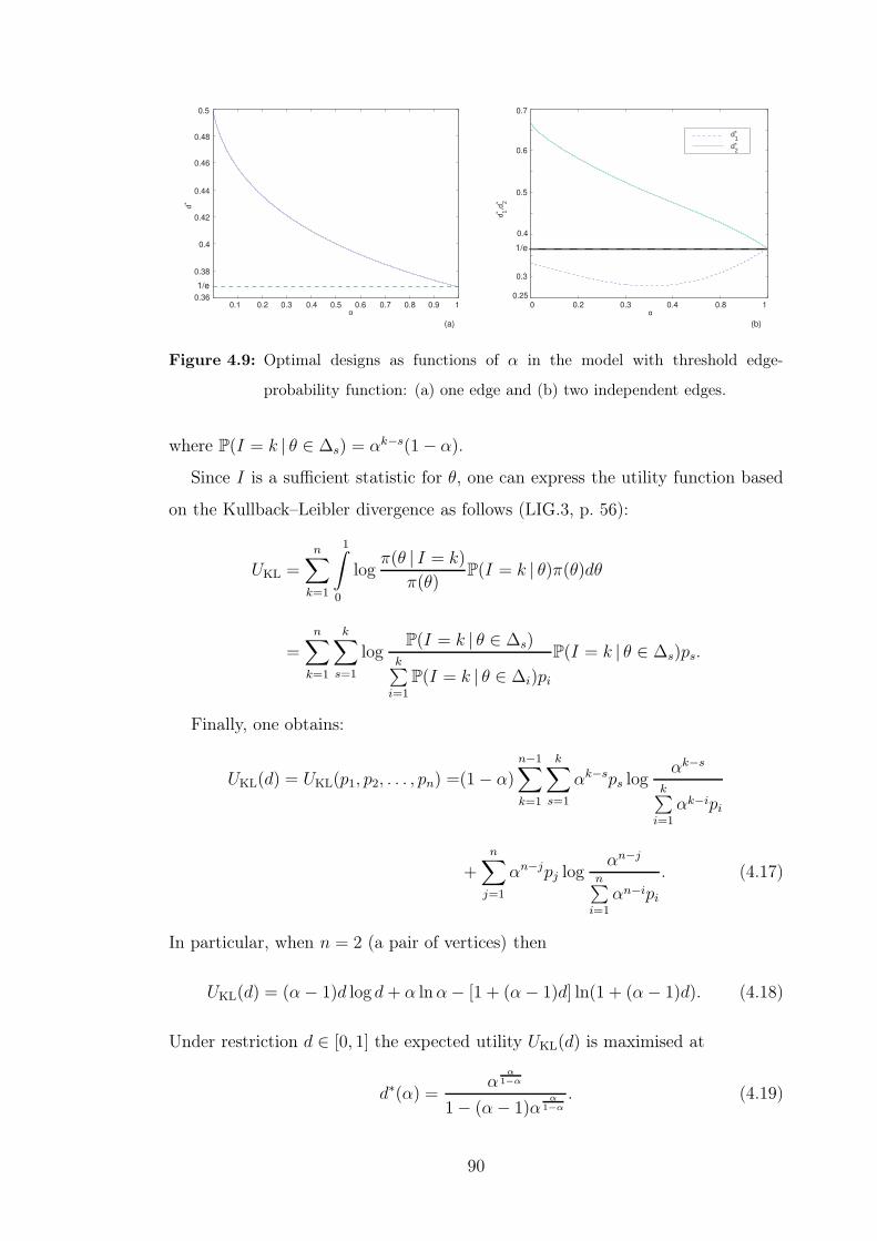
1/e
1/e
0.7
0.6
0.5
0.4
0.3
0 0.2 0.3 0.4 0.8 10.25
d 1,d2
α
d1*
*d2
*
*
(b)
0.360.1 0.2 0.3 0.4 0.5 0.6 0.7 0.8 0.9 1
0.38
0.42
0.44
0.46
0.48
0.5
0.4
α
d*
(a)
Figure 4.9: Optimal designs as functions of α in the model with threshold edge-
probability function: (a) one edge and (b) two independent edges.
where P(I = k | θ ∈ ∆s) = αk−s(1− α).
Since I is a sufficient statistic for θ, one can express the utility function based
on the Kullback–Leibler divergence as follows (LIG.3, p. 56):
UKL =n∑
k=1
1∫
0
logπ(θ | I = k)
π(θ)P(I = k | θ)π(θ)dθ
=
n∑
k=1
k∑
s=1
logP(I = k | θ ∈ ∆s)
k∑i=1
P(I = k | θ ∈ ∆i)pi
P(I = k | θ ∈ ∆s)ps.
Finally, one obtains:
UKL(d) = UKL(p1, p2, . . . , pn) =(1− α)
n−1∑
k=1
k∑
s=1
αk−sps logαk−s
k∑i=1
αk−ipi
+n∑
j=1
αn−jpj logαn−j
n∑i=1
αn−ipi
. (4.17)
In particular, when n = 2 (a pair of vertices) then
UKL(d) = (α− 1)d log d+ α lnα− [1 + (α− 1)d] ln(1 + (α− 1)d). (4.18)
Under restriction d ∈ [0, 1] the expected utility UKL(d) is maximised at
d∗(α) =α
α1−α
1− (α− 1)αα
1−α
. (4.19)
90

Figure 4.9(a) shows the plot of d∗(α). Interestingly enough to notice that
limα→1
d∗(α) = 1/e. (4.20)
For general n and α the problem of optimal design for the model with thresh-
old edge-probability function can be solved by numerically solving the following
optimisation problem:
Maximise UKL(p1, p2, . . . , pn), (4.21)
subject ton∑
i=1
pi = 1, (4.22)
pi ≥ 0, i = 1, . . . , n, (4.23)
where UKL(p1, p2, . . . , pn) is taken in the form (4.17).
When n = 3 there are two independent edges of lengths d1 and d2. Figure 4.9(b)
represents 2-edge optimal designs d∗1 and d∗2 as functions of α.
Table 4.1 contains optimal designs which correspond to different values of α
from the interval [0,1) in the case of 3 independent edges (n=4). Notably, the
optimal designs seem to be planar for any α in this case (but one should keep
in mind that θ was taken to be uniformly distributed, and if we reparametrise
the model by accordingly transforming θ and its support, the optimal design can
be obtained as corresponding quantiles of the new prior distribution of θ and the
planarity may be easily ‘violated’ by such procedure.).
Figure 4.9 and Table 4.1 were obtained by solving numerically the optimisation
problem (4.21) with linear constraints (4.22) and (4.23).
Finally notice that it looks very convincing from Figure 4.9 and Table 4.1 that
optimal edge lengths d∗i (α), i = 1, . . . , n, tend to 1/e ≈ 0.368 each, as α goes to 1.
We currently do not have analytic proof of this for general values of n.
4.2.6 Non-preservation of optimal designs under replication
Although optimal designs are often maintained under replication in the case of
linear (or linearisable) models with normal errors, the following trivial example
91

α d1 d2 d3
0.0 0.25 0.5 0.75
0.1 0.2499 0.4759 0.7132
0.2 0.2481 0.4526 0.6872
0.3 0.2435 0.4278 0.6604
0.4 0.2378 0.4040 0.6298
0.5 0.2344 0.3840 0.5967
0.6 0.2365 0.3702 0.5615
0.7 0.2468 0.3633 0.5238
0.8 0.2691 0.3625 0.4819
0.9 0.3077 0.3654 0.4319
Table 4.1: Optimal designs for the model with threshold edge-probability function as
functions of the threshold α when n = 4.
shows that this is not generally true. A related point that this example shows is
that the sequential optimal design of replicated experiments need not be the same
as the optimal design of simultaneous replicated experiments.
The following elementary proof is given in Cook et al. (2008) and appeared in
discussion with Alex Cook. It uses the results for optimal designs for geometric
random graphs discussed in § 4.2.4.
Imagine the following situation. There are two replicate populations of n in-
dividuals each. Individuals pass from state S to state I after a constant period
of time µ. Replicate A is observed once at time τA and replicate B once at time
τB. Without loss of generality, τA ≤ τB. Let Ii(t) be the number of individuals
in replicate i in the state I at time t. Clearly, Ii(t) = 0 if t < µ and Ii(t) = n if
t ≥ µ.
Assume that the prior knowledge for µ is vague and expressed via the following
prior distribution:
π(µ) = 1l{µ∈(0,1)}.
Let us restrict our attention to the designs such that τi ∈ [0, 1], since any other
design would yield no more information.
92

The uniform prior π(µ) translates to the following priors for {IA(τA), IB(τB)}:
P ({IA(τA), IB(τB)} = (0, 0)) = 1− τB (4.24)
P ({IA(τA), IB(τB)} = (n, 0)) = τB − τA (4.25)
P ({IA(τA), IB(τB)} = (n, n)) = τA, (4.26)
with the outcome in (4.25) having probability 0 if an identical choice of design in
the two replicates is made, i.e. if τA = τB.
It follows that the posterior for µ is:
π(µ | {IA(τA), IB(τB)} = (0, 0)) =1
1− τB1l{µ∈(τB ,1)} (4.27)
π(µ | {IA(τA), IB(τB)} = (n, 0)) =1
τB − τA1l{µ∈(τA ,τB)} (4.28)
π(µ | {IA(τA), IB(τB)} = (n, n)) =1
τB − τA1l{µ∈(τ0,τA)}. (4.29)
If τA < τB, the expected utility, based on the Kullback–Leibler divergence, is
E [U(τA, τB)] = (1− τB) log1
1− τB+ (τB − τA) log
1
τB − τA+ τA log τ−1
A , (4.30)
which is maximised (Theorem 4.2.2) by (τA, τB) = (1/3, 2/3), with the expected
information yield U(1/3, 2/3) = log 3.
If, on the other hand, τA = τB = τ, the expected utility becomes
E [U(τ, τ)] = (1− τ) log1
1− τ− τ log τ, (4.31)
which is maximised by τ = 1/2, giving utility U(1/2, 1/2) = log 2 < U(1/3, 2/3).
In fact, it can readily be seen that taking the same design in both replicates
yields no more information than having a single replicate with that design. It can
also be seen that replicates containing a single individual yield the same infor-
mation as those containing more than one individual. It seems to be intuitively
obvious that if the lifetimes are random and their variance is much smaller than
the variance of the prior for the mean, a similar result will hold.
93

A related point that this example shows is that the sequential optimal design of
replicated experiments need not be the same as the optimal design of simultaneous
replicated experiments. If we ran the above experiment simultaneously, the best
design, as found above, is τA = 1/3 and τB = 2/3 with the utility equal log 3.
If, however, we allowed the inference which results from replicate A to be used
for designing an experiment B at some later time, an argument similar to that
above shows that the optimal design is to take τA = 1/2, followed by τ = 1/4 if
IA(1/2) = n, and τB = 3/4 if IA(1/2) = 0. This sequential design has utility log 4
and thus is more informative than the simultaneous design.
94

Chapter 5
Lattice-based Optimal Designs
In the first section of this chapter we study inference and optimal design problems
for finite clusters from percolation on the integer lattice Zd or, equivalently, for
SIR epidemics evolving on a bounded subset of Zd with constant infectious times.
The corresponding percolation probability p is considered to be unknown, possibly
depending, through the experimental design, on other parameters. We consider
inference under each of the following two scenarios:
(i) The observations consist of the set of sites which are ever infected, so that
the routes by which infections travel are not observed (in terms of the bond
percolation process, this corresponds to a knowledge of the connected com-
ponent containing the initially infected site—the location of this site within
the component not being relevant to inference for p).
(ii) All that is observed is the size of the set of sites which are ever infected. By
the set size we mean cardinality here.
We discuss practical aspects of Bayesian utility-based optimal designs for the
former scenario and prove that the sequence of maximum likelihood estimates for p
converges to the critical percolation probability pc under the latter scenario (when
the size of the finite cluster grows infinitely).
In the second section we outline how the results for nearest-neighbour graph
models can be generalised to the case of long-range connections.
95

5.1 Inference and Optimal Design for Percolation
Models
5.1.1 Nearest-neighbour interaction model and percolation
Brief historical account on percolation
The concept of percolation has received enormous interest among physicists since
it was introduced by Broadbent and Hammersley (1957). One reason for that,
perhaps, is that it provides a clear and intuitively appealing model of the geom-
etry which appears in disordered systems. Percolation has been used to model
and analyse the spreading of oil in water and transport phenomena in porous me-
dia and materials (Yanuka (1992), Stauffer and Aharony (1992), de Gennes and
Guyon (1978), Larson et al (1981), Sahimi (1994), Odagaki and Toyufuku (1998),
Tobochnik (1999), De Bondt et al (1992), Bunde et al (1995), Bentz and Gar-
boczi (1992), Machta (1991), Moon and Girvin (1995)), to model the spread of in-
fections and forest fires via nearest and finite range percolation (Zhang (1993), Cox
and Durrett (1988), Gibson et al (2006)) and via continuum percolation (Meester
and Roy (1996)). It has also been used in studying failures of electronic de-
vices and integrated circuits (Gingl et al (1996)), in modelling random resistor
networks (Pennetta et al (2002)), and in studying transport and electrical prop-
erties of percolating networks (Adam and Delsanti (1989)). Percolation models
have also been used outside physics to model ecological disturbances (With and
Crist (1992)), robustness of the Internet and other networks (Cohen et al (2000),
Callaway et al (2000)), biological evolution (Ray and Jan (1994)), and social in-
fluence (Solomon et al (2000)). Percolation is one of the simplest models which
exhibits phase transition, and the occurrence of critical phenomena is central to
the appeal of percolation. The reader is referred to Chapter 1 of Grimmett (1999)
for further details on modelling a random medium using percolation models.
96

Classical SIR epidemic model and percolation
Disease spread as a result of (typically) short-range contact between, for example,
plants can be modelled as a transmission process on an undirected graph. Nodes,
or vertices, of the graph correspond to possible locations of plants, and edges of
the graph link locations which are considered to be neighbours. In a classical SIR
model each node, or vertex, of the graph is in one of three states: either it is
occupied by a healthy, but susceptible, plant (state S ), or it is occupied by an
infected and infectious plant (state I ), or finally it is empty, any plant at that
location having died and thus being considered removed (state R). A plant at
node i, once infected (or from time 0 if initially infected), remains in the infected
(and infectious) state I for some random time τi after which it dies, so that node
i then remains in the empty state R ever thereafter. During its infectious time
the plant at node i sends further infections to each of its neighbouring nodes j as
a Poisson process with rate λij (so that the probability that an infection travels
from i to j in any small time interval of length h is λijh + o(h) as h → 0 while
the probability that two or more infections travel in the same interval is o(h) as
h → 0); any infection arriving at node j changes the state of any healthy plant
there to infected, and otherwise has no effect. All infectious periods and infection
processes are considered to be independent of each other. The initial state of the
system is typically defined by one or more nodes being occupied by infected plants,
the remaining nodes being occupied by healthy plants. The epidemic may die out
at some finite time at which the set of infected nodes first becomes empty, or, on
an infinite graph only, it is possible that it may continue forever.
Thus, for any infected node i, the event Eij that any neighbouring node j re-
ceives at least one infection from node i has probability pij = 1 − E[exp(−λijτi)](here, as previously, E denotes expectation). Note that, for any given node i, even
though the infection processes are independent, the events Eij are themselves in-
dependent if and only if the random infectious period τi is a constant. We now
suppose that this is the case and that furthermore, for all ordered pairs (i, j) of
neighbours, we have pij = p for some probability p. Suppose further that it is
possible to observe neither the time evolution of the epidemic nor the edges of
97

the graph by which infections travel, but only the initially infected set of nodes
and the set of nodes which are at some time infected and thus ultimately in the
empty state R. It is then not difficult to see, and is indeed well known (e.g. Ku-
ulasmaa and Zachary (1984)), that the epidemic may be probabilistically realised
as an unoriented bond percolation process on the graph in which each edge is in-
dependently open with probability p, and in which the set of nodes which are
ever infected consists of those nodes reachable along open paths (chains of open
edges) from those initially infected. (Note that the ability to use an unoriented
bond percolation process requires both the assumptions that the above events Eij
are independent and that pij = pji for all i, j; in the absence of either of these
assumptions one would in general need to consider an oriented process with the
appropriate dependence structure 1.)
Further we consider the epidemic to take place on some subset Π of the two-
dimensional integer lattice Zd, where we allow Π = Z
d as a possibility. Two sites
(nodes) are considered neighbours if and only if they are distance 1 apart. Thus
in the case Π = Z2 each node has 4 neighbours. This may be considered as a
model for nearest-neighbour interaction. We assume furthermore that initially
there is a single infected site, and that all other sites in Π are occupied by healthy
individuals.
Bond percolation in graph-theoretic terms
We now establish the basic definitions and notation for bond and site perco-
lation on the integer lattice. As usual, we write Zd for the set of all vectors
x = (x1, x2, . . . , xd) with integer coordinates. The norm ‖ · ‖1 defines a distance
between each two elements of Zd, x and y, as follows:
δ(x, y) :=‖ x− y ‖1=d∑
i=1
|xi − yi|.
1Non-constant infectious period distributions τi can similarly lead to other interesting per-
colation processes. For example, site percolation may be approximated arbitrarily closely by
an infectious period distribution which with some sufficiently small probability takes some suffi-
ciently large value, and which otherwise takes the value zero (see Appendix E).
98

The set Zd may be turned into a graph using the ‘4-neighbourhood relationship’
as follows: two elements x and y are declared to be neighbours (or adjacent) if
and only if δ(x, y) = 1. If x and y are adjacent, then we write x ∼ y. The set of
edges obtained in this way is denoted by Ed and the corresponding graph (Zd,Ed)
is called the d-dimensional cubic lattice (Grimmett (1999)). We denote this lattice
by Ld and the origin of Zd by 0.
The following describes the percolation process on Ld. Let p be a real number
between zero and one: 0 ≤ p ≤ 1. We declare each edge of the lattice Ld to be
open with probability p and closed otherwise, independently of the status of any
other edge. The random subgraph of Ld formed in this way contains the vertex set
Zd and the open edges only. The connected components of this graph are called
open clusters. The open cluster containing the vertex x is denoted by C(x). It
is clear that the distribution of C(x) is independent of the choice of x. The open
cluster C := C(0) containing the origin is typical in this sense. Figure 5.1 depicts
examples of open clusters of a percolation process on L2 (for different values of p)
restricted to the bounding box [−31, 31]× [−31, 31].
A central quantity of interest in percolation theory is that of percolation prob-
ability θ(p), this being the probability that the origin (or any other given vertex)
belongs to an infinite open cluster:
θ(p) := Pp(|C = ∞|) = 1−∞∑
n=1
Pp(|C| = n).
The following critical phenomenon results are of fundamental importance in per-
colation theory (Grimmett (1999)):
• The function θ is a non-decreasing function of p:
0 = θ(0) ≤ θ(p′) ≤ θ(p′′), ∀p′, p′′ : 0 ≤ p′ ≤ p′′ ≤ 1.
• There exists a critical value pc(d) of p such that θ(p) = 0 for any p < pc(d) and
θ(p) > 0 for any p > pc(d). The value pc(d) is called the critical probability
and can formally be defined as follows:
pc(d) := sup{p : θ(p) = 0}.
99

(a) (b)
(c) (d)
(e) (f)
Figure 5.1: Open clusters emerged as a result of bond percolation on L2 for different
values of p: (a) p = 0.2, (b) p = 0.4, (c) p = 0.5, (d) p = 0.6, (e) p = 0.75,
and (f) p = 0.9. The origin of Z2 is denoted by a circle in the centre of
each plot. 100

• The critical probability is unity in the one-dimensional case: pc(1) = 1.
• The critical probability exists and is strictly between zero and one on the
lattice Ld, d ≥ 2:
0 < pc(d) < 1, for any d ≥ 2.
• The critical probability is a monotonically decreasing function in d:
pc(d+ 1) < pc(d), for d ≥ 1.
Incomplete observations
The probability p introduced above is considered to be unknown, but may depend
on other parameters. For instance, this probability may depend on the distance
between plants (lattice vertices) or, if Π = Z2 and the Poisson process of emitting
germs by infectious plants is isotropic, it may be related to its intensity λ = 4λij
(each site has four neighbours in L2). In the latter case p may be taken to be of
the form p = 1 − e−λ/4 and it is λ that would be an object of interest for plant
epidemiologists.
We consider inference under each of the following two scenarios:
(i) the observations consist of the set of sites which are ever infected, so that the
routes by which infections travel are not observed; note that, in terms of the
bond percolation process, this corresponds to knowledge of the connected
component containing the initially infected site—the location of this site
within the component not being relevant to inference for p (see below);
(ii) all that is observed is the size of the set of sites which are ever infected.
We denote and refer further to the former of these two scenarios as S1 and to
the latter scenario as S2.
5.1.2 Parameter estimation
Distribution of ever-infected sites
Consider our SIR constant infectious period epidemic on a locally finite graph in
which the probability that any individual i sends at least one infection to any given
101

neighbour j is p. By the definition of the epidemic these events are independent.
The following basic result is well-known. However, the author was unable to
find a reference to the formulated and rigorously proven result—this theorem can
be well regarded as a part of mathematical folklore of the sort “It is easy to see
that...” (e.g., see Grassberger (1983)).
Theorem 5.1.1. For any given set of initially infected sites, the distribution of
the set of ever-infected sites is the same as for the corresponding unoriented bond
percolation process (with the same initial set).
Proof. Given the realisation of the epidemic we construct a realisation of the unori-
ented bond percolation process as follows. For each unordered pair of neighbours
{i, j}, if i, say, becomes infected before j then we construct an open link between
i and j if and only if, in the epidemic, i sends at least one infection to j; if either
i and j are both initially infected or i and j are both never infected, then we
construct an open link between i and j with probability p independent of all else.
Since the probability for two vertices to become infected at exactly the same time
is 0, it is clear from consideration of the temporal evolution of the epidemic that
all edges are open with probability p independently of each other. Furthermore,
the set of ever-infected sites in the epidemic is the same as the set of ‘wetted’
sites (sites linked by open edges to the initial wet set) in the bond percolation
process.
It follows that, for inference, if all that is observed is the set of ever-infected
sites, then we may calculate the likelihood function using the unoriented bond
percolation model. However, one cannot think of any scenario in which we also
obtain any information about the links used to spread the epidemic for which a
similar conclusion holds. Here are two possible scenarios with counter-examples.
• For at least some unordered pairs {i, j} of neighbours, we observe whether or
not an infection passed between i and j (even if both were already infected).
Consider the graph with 2 vertices and one edge, and suppose we observe
the edge to have been used; then the likelihood for the epidemic model is
2p− p2, while that for the unoriented bond percolation model is p.
102

Figure 5.2: An open cluster (black solid dots) containing the origin (a black dot in a
circle) as a result of percolation simulation on L2. Here the bond perco-
lation probability p was taken to be 0.478; the solid bonds represent open
bonds. The open cluster can be seen as a finite outbreak of an epidemic
with constant infectious periods and infection intensity spread rate λ ≈ 2.6
evolving on Π = Z2 (since 0.478 = 1 − e−2.6/4). The dotted lines depict
directions along which infection did not spread (from black to grey dots);
thus, grey dots depict individuals which remain healthy and the dotted lines
represent those bonds that must be absent given knowledge of the cluster
set.
• For at least some ordered pairs (i, j) of neighbours, we observe whether or
not an infection passed from i to j (even if j was already infected). Consider
the graph with 3 vertices and 3 edges, and suppose (with vertex 1 initially
infected) we observe infections to have passed from 1 to 2 and from 1 to 3
and also that no other infections have passed; then the likelihood for the
epidemic model is p2(1− p)4, while that for the unoriented bond percolation
model is p2(1− p).
In the first of the above scenarios, if we made the observation for every unordered
pair of neighbours, then, for inference, we could pass to the unoriented bond
percolation model with parameter p′ = 2p− p2.
The result proved in Theorem 5.1.1 means that a final snapshot of an SIR epi-
demic with nearest-neighbour interaction and constant infectious periods evolving
on Z2 can be seen as an open cluster of the corresponding percolation process on
L2 = (Z2,E2), had the infection process started with a single initially inoculated
103

site (placed at the origin of the lattice, for example). Figure 5.2 shows an open
cluster obtained by simulation of percolation process on the integer lattice in plane
when p = 0.478. This connected component containing the origin can be seen as a
final (and finite) outbreak of an SIR epidemic process of the kind discussed above.
The origin (or, indeed, any other vertex of the open cluster) may be considered to
be the site where the initially inoculated individual has been placed. Clearly, the
realised bond structure is not the only possible way resulting in the site configu-
ration seen in Figure 5.2. However, the distribution of this site configuration as
an extinct SIR epidemic coincides with that of the corresponding unoriented bond
percolation process.
Scenario S1: hidden bond structure
Let Π be a (proper or improper) subgraph of Ld = (Zd,Ed) containing the origin
and let C be an open cluster of a percolation process on the graph Π containing
the origin. The set of nodes C represents a snapshot of an extinct outbreak of our
spatial SIR epidemic evolving on Π ⊆ L2.
Let us introduce some additional notions. Let G = (V,E) be a locally finite
graph and let G′ = (V ′, E ′) be a subgraph of G. By the saturation of the graph
G′ with respect to G we understand the graph G = (V , E) such that
V = V ′ and E = {(x, y) | x, y ∈ V ′ & (x, y) ∈ E}.
Thus, in order to obtain the saturation of a subgraph G′ of a given graph G one
needs to add to G′ all possible edges from G with endpoints from G′, and hence
‘saturate’ it.
We denote the saturation of G′ with respect to G by SaturGG′ or, in cases when
it is clear from the context with respect to what graph the saturation takes place,
by SaturG′. A graph G′ whose saturation (with respect to some graph G) coin-
cides with itself is called a fully saturated graph. For example, the fully saturated
graph (with respect to L2) is obtained from the graph depicted in Figure 5.2 by
connecting all pairs of neighbouring black sites (according to the 4-neighbourhood
relationship). Note that the operation of saturation may also be applied solely to
a subset of vertices of the original graph, since it does not make use of the edges
104

of the subgraph-operand (alternatively, one may think about the subset of the
original graph vertex set as a subgraph with an empty edge set).
In order to distinguish between the boundary points of a graph and their neigh-
bours, which are not in the graph, we introduce the notions of the surface and the
frontier of the graph (again, with respect to another graph). Let us denote by ∂G
the surface of G in Π, G ⊆ Π, that is to say the set
∂G := {x ∈ G : ∃y ∈ Π\G such that x and y are neighbours in Π},
and by ΓG the frontier of G in Π, i.e. the set ∂(Π\G).In order to identify the likelihood function we introduce the set G(C) of all con-
nected subgraphs of Π with C as a vertex set. Note that the set G(C) is necessarily
nonempty. For each G ∈ G(C) the number of edges between the vertices of the
graph G and the elements of its frontier ΓG is the same—we denote it by wC.
Finally, we denote the total number of edges present in G by e(G).
The probability that C represents the set of ever-infected sites and that the
edges of G correspond to those routes along which the infection travelled is
Pp(G) = pe(G)(1− p)e(Satur C)−e(G)+wC ,
and the likelihood function associated with the observed set C of ever-infected sites
is given by
L(p) = Pp(C) =∑
G∈G(C)Pp(G).
Hence, under assumption of a uniform prior for p, its posterior distribution
π(p | C) is a mixture of beta distributions:
π(p | C) ∝∑
k
r(k)Beta (k + 1, e(Satur C)− k + wC + 1) ,
where
r(k) := #{G ∈ G(C) | e(G) = k}.
It is not feasible to calculate π(p | C) in the above form for reasons of difficulty
in calculating efficiently the coefficients r(k), since it is hard to enumerate all
corresponding graphs. We describe therefore an MCMC algorithm that allows
105

0 0.2 0.4 0.6 0.8 10
200
400
600
800
1000
1200
1400
1600
p
Figure 5.3: Solid line corresponds to the likelihood function evaluated for the complete
information (both the site and edge configurations are known) on the cluster
C from Figure 5.2. The histogram is based on a sample drawn from the
MCMC applied to the site configuration C (nodes only).
one to sample from the distribution π(p | C) under the uniform prior on p, that is,
effectively, to evaluate the likelihood function of p.
Our Markov chain explores the joint space of values for p and graphs from G(C),that is to say the set [0, 1]× G(C). The stationary distribution of the chain is the
joint posterior distribution of p and G ∈ G(C). The description of the chain is
given in Algorithm 1. This Markov chain explores the set of all connected graphs
G(C) by simply deleting or adding an edge from the current graph preserving the
connectivity of the given site configuration C.
The proposed MCMC is irreducible by construction: there is a positive proba-
bility for the chain to switch between any two connected graphs from G(C) since
any two such graphs have the same vertex set and differ by a finite number of
edges only.
Example 5.1.2. We apply Algorithm 1 to the site configuration C from Figure 5.2
(black dots only). This open cluster at the origin was obtained by simulating the
percolation process in Z2 using the value of the percolation parameter p = 0.478.
106

Algorithm 1 Markov Chain Monte Carlo: scenario S1Require: an open cluster C;
1: take an initial value p0 arbitrary from (0, 1);
2: t := 0 Xt := (pt, Satur C);3: repeat
4: Gibbs sampler steps:
5: p2t+1 ∼ Beta (e(G2t) + 1, e(Satur C)− e(G2t) + wC + 1);
6: X2t+1 := (p2t+1, G2t);
7: Metropolis–Hastings sampler steps:
8: choose an edge e uniformly at random from Satur C;
9: if e ∈ G2t then
10: U ∼ Uniform[0, 1];
11: if U ≤ min(1, 1−p2t+1
p2t+11l{G2t+1\{e} is connected}) then
12: X2t+2 := (p2t+1, G2t+1 \ {e});13: else
14: X2t+2 := (p2t+1, G2t+1);
15: else
16: U ∼ Uniform[0, 1];
17: if U ≤ min(1, p2t+1
1−p2t+1) then
18: X2t+2 := (p2t+1, G2t+1 ∪ {e});19: else
20: X2t+2 := (p2t+1, G2t+1);
21: t := t + 2;
22: until we judge that the chain has converged and a sample of sufficient size is
recorded
107

0 2000 4000 6000 8000 100000.2
0.25
0.3
0.35
0.4
0.45
0.5
0.55
0.6
0.65
step
Figure 5.4: Trace plot for MCMC sampling resulted in the histogram from Figure 5.3
for the cluster C from Figure 5.2. The trace plot indicates that the mixing
properties of the chain are rather satisfactory. It took 28 seconds on Intel(R)
Core(TM)2 Duo CPU 2.26GHz to obtain a series of chain updates of the
length 104. This time could be further reduced by using dynamic graph
update algorithms, see the footnote on the p. 129.
Figure 5.3 shows the likelihood function of the model parameter for the complete
observation (i.e. nodes and edges of the cluster) and a histogram of a sample from
the posterior distribution π(p | C) obtained by running the MCMC described in Al-
gorithm 1 when the prior distribution is uniform on the interval (0, 1).
An animated example of using Algorithm 1 can be found at the WEB address
http://www.cl.cam.ac.uk/~aib29/HWThesis/Video/. We defer the discussion
on the mixing properties of the suggested chain until § 5.1.4.
Scenario S2: unknown site configuration
Under this scenario only the size n of the outbreak of our SIR epidemic evolving
on Π = Ld is given.
Let Gn be the set of all possible connected graphs on n vertices including the
origin. These graphs represent the outbreaks of the size n and we distinguish all
isomorphic graphs which have different orientation.
108

We denote the number of edges of Π between the vertices of the graph G ∈ Gn
and the vertices of its frontier ΓG by w(G).
Given the epidemic of size n, the inference on p involves evaluation of the
likelihood function Ln(p) := Pp(|C| = n) which can be represented as follows:
Ln(p) =∑
G∈Gn
Pp(G).
As previously, under assumption of a uniform prior for p its posterior distribution
π(p | |C| = n) is a mixture of beta distributions:
π(p | |C| = n) ∝∑
s,k,l
q(s, k, l)Beta (k + 1, s− k + l + 1) , (5.1)
where
q(s, k, l) := #{G ∈ Gn | e(SaturG) = s, e(G) = k, w(G) = l}.
This, again, represents a hard enumeration problem. However, inference on p
can be made using the MCMC technique. Algorithm 2 contains a description of a
Markov chain which serves the purpose of sampling from the posterior distribution
π(p | |C| = n), given the prior distribution of p is uniform on [0,1]. The chain
explores the joint space of all possible connected graphs on n nodes and possible
values for the percolation parameter p by deleting a vertex from the current graph
and adding a vertex from its frontier.
The presented Markov Chain Monte Carlo algorithm, similarly to the one sug-
gested for the previously considered scenario S1, is a combination of Gibbs and
Metropolis–Hastings steps. The marginal of the chain limiting distribution f(p,G)
in p coincides with the posterior distribution π(p | |C| = n).
We give now explicit expressions for the proposal probabilities used in the
Metropolis–Hastings part of this algorithm. Assume that the current graph within
the Metropolis–Hastings step is G and a graph G is proposed, the latter being ob-
tained from the former by deleting a vertex u with all edges adjoining it and
inserting a vertex v with every possible edge, each independently with probability
p, which was determined by the preceding Gibbs step. We assume that at least
one such edge is inserted and denote the number of deleted and added edges by
109

Algorithm 2 Markov Chain Monte Carlo: scenario S2Require: the value of n.
1: take a value p0 arbitrary from (0, 1) and a graph G0 arbitrary from Gn;
2: t := 0 Xt := (pt, Gt);
3: repeat
4: move_on:=1;
5: Gibbs sampler steps:
6: p2t+1 ∼ Beta (e(G2t) + 1, e(SaturG2t − e(G2t) + w(G2t) + 1));
7: X2t+1 := (p2t + 1, G2t);
8: Metropolis–Hastings sampler steps:
9: choose a vertex u uniformly at random from G2t+1 and choose a vertex v
uniformly at random from ΓG2t+1. Derive a graph G from G2t+1 by deleting
all edges which adjoin u (in G2t+1) and adding the edges that connect v with
vertices of the graph G2t+1 \ {u} in Π, each independently with probability
p2t+1 (conditioning on the event that at least one edge is added).
10: if G is disconnected then
11: X2t+2 := (p2t+1, G2t+1); move_on:=0
12: if move_on then
13: U ∼ Uniform(0, 1);
14: d(v) := #{e | e = (v, z) ∃z ∈ G2t+1 \ {u}};15: d(u) := #{e | e = (u, z) ∃z ∈ G \ {v}};16: ν(u) := #{x | x ∈ ΓG2t+1 & (u, x) ∈ Π};17: ν(v) := #{x | x ∈ ΓG & (v, x) ∈ Π};18: κ := d(u)− d(v) + ν(v)− ν(u); U ∼ Uniform(0, 1);
19: if U ≤ min(1,
|ΓG2t+1|
|ΓG|1−(1−p2t+1)d(v)
1−(1−p2t+1)d(u)(1− p2t+1)
κ)
then
20: X2t+2 := (p2t+1, G);
21: else
22: X2t+2 := (p2t+1, G2t+1);
23: t := t + 2;
24: until we judge that the chain has converged and a sample of sufficient size is
recorded
110

d(u) and d(v) respectively. Then,
q(G, G) =1
n
1
|ΓG|pd(v)(1− p)d(v)−d(v)
1− (1− p)d(v)1l{G is connected}, (5.2)
and similarly,
q(G, G) =1
n
1
|ΓG|pd(u)(1− p)d(u)−d(u)
1− (1− p)d(u)1l{G is connected}. (5.3)
Clearly,
Pp(G) ∝ pd(u)(1− p)d(v)(1− p)d(u)−d(u)+ν(u)
Pp(G) ∝ pd(v)(1− p)d(v)(1− p)d(v)−d(v)+ν(v) ,
so that the acceptance probability at the Metropolis–Hastings step, α, is as follows:
α = min
(1,q(G, G)
q(G, G)
Pp(G)
Pp(G)
)
= min
(1,
|ΓG||ΓG|
(1− p)d(u)+ν(v)
(1− p)d(v)+ν(u)
1− (1− p)d(v)
1− (1− p)d(u)
)
= min,
(1,
|ΓG||ΓG|
1− (1− p)d(v)
1− (1− p)d(u)(1− p)κ
),
where, as it was introduced in the description of Algorithm 2,
κ := d(u)− d(v) + ν(v)− ν(u).
We claim that the constructed chain is irreducible, that is to say this chain can
get from each state to any other state. In graph theory notions this means that the
chain can get from each connected graph on n vertices including the origin to any
other connected graph on n vertices (also including the origin) on the considered
lattice. We show the irreducibility of the proposed MCMC by constructing a
sequence of steps in which any graph of Gn is transformed to a so called line-
skeleton graph on n vertices. By such a graph we mean any tree (a graph with
no cycles) containing the origin of the lattice and having n vertices so that only
two of these vertices have degree one. Choose and fix one of such line-skeletons
denoting it by S.
111

Consider a graph G from Gn and denote the length of the shortest path from
x ∈ G to S by δ(x, S) (δ here is the distance introduced in § 5.1.1). Each vertex x
from G receives a well defined finite weight δ(x, S), since the graph G is connected
and finite. By using the description of our Markov chain we can delete any vertex
from our current graph for which δ(x, S) is maximal and add to this graph a
vertex from the chosen line skeleton S without making the graph disconnected
or containing cycles until the maximum value of d(x, S) is zero—in this case all
vertices are forming the line skeleton. Since this procedure can be reversed it
follows that Gn in the described Markov chain is indeed a communicating class,
and hence the chain is irreducible.
An animated example of using Algorithm 2 when n = 25 can be found at the
WEB address http://www.cl.cam.ac.uk/~aib29/HWThesis/Video/. Figure 5.5
shows histograms of samples from the distribution π(p | |C| = n) obtained using the
proposed MCMC for the scenario S2 for the cluster size values p = 10, 35, 50, 70
and corresponding trace plots.
In realisations of either of the described algorithms (Algorithm 1 and Al-
gorithm 2) we used the MATLAB library MatlabBGL (http://www.stanford.
edu/~dgleich/programs/matlab_bgl/) for checking connectivity of the proposal
graphs.
Convergence of inferences for S2 with increasing cluster size
Percolation exhibits a phenomenon of criticality, this being central in the percola-
tion theory: as p increases, the sizes of open clusters (connected components) also
increase, and there is a critical value of pc at which there appears a cluster which
dominates the rest of the pattern. Loosely speaking, as more and more edges
are assigned to be open, there comes a moment when large-scale connections are
formed across the lattice. If p < pc, then with probability one all open clusters
are finite, but there is a single infinite open cluster when p > pc almost surely.
The bond percolation on the square lattice seems to be most studied to date of
all percolation processes. The critical probability pc in the case of a square lattice
is 12. What follows, however, holds for any lattice Z
d, d ≥ 2.
112

3000 3500 4000 4500 50000.1
0.2
0.3
0.4
0.5
0.6
0.7
0.8
0.1 0.2 0.3 0.4 0.5 0.6 0.7 0.80
50
100
150
200
250
300
350
400
450
500
0.2 0.25 0.3 0.35 0.4 0.45 0.5 0.55 0.6 0.650
100
200
300
400
500
600
0.2 0.25 0.3 0.35 0.4 0.45 0.5 0.55 0.6 0.650
100
200
300
400
500
600
700
800
900
1000 2000 3000 4000 5000 6000 7000 80000.2
0.25
0.3
0.35
0.4
0.45
0.5
0.55
0.6
0.65
3000 3500 4000 4500 50000.2
0.25
0.3
0.35
0.4
0.45
0.5
0.55
0.6
0.65
0.25 0.3 0.35 0.4 0.45 0.5 0.55 0.6 0.650
100
200
300
400
500
600
700
800
900
1000 2000 3000 4000 5000 6000 7000 8000 9000 100000.2
0.25
0.3
0.35
0.4
0.45
0.5
0.55
0.6
0.65
(a) (b)
(c) (d)
(e) (f)
(g) (h)
Figure 5.5: Inference on the percolation parameter using MCMC described in Algo-
rithm 2: histograms of obtained samples and trace plots for (a,b) n = 10;
(c,d) n = 35; (e,f) n = 50; (g,h) n = 70.
113

As before, denote by C(x) the open cluster (connected component) which con-
tains the vertex x. Let us write χ(p) = Ep|C| for the mean number of vertices
in the open cluster C := C(0) at the origin. Using the translation invariance of
the process on Zd, we have χ(p) = Ep|C(x)| for all vertices x. The percolation
theory tells us that if p < pc, then χ(p) < ∞ (Grimmett (1999, p. 20)). When
p > pc, then χ(p) = ∞ and the function χ is not of a much interest in this case.
Instead, one studies the function χf(p) = Ep[|C| : |C| < ∞]. The function χ(p)
(χf (p)) monotonically increases as p ↑ pc (p ↓ pc), having p = pc as its asymptote.
It is known that there is no infinite open cluster when p = pc for percolation on
the square lattice. How likely it is to observe an open cluster of size n when n is
very large? What value of p should one suggest if one happened to observe a large
epidemic of size n?
It is intuitively unlikely that if p is much smaller than pc (p ≪ pc) or much
larger than this value (p≫ pc) that, having attained a sufficiently large size n, the
epidemic would have burned out. Intuition suggests therefore that the likelihood
function for p, given that the size n of the connected component containing the
origin is increasing, should be increasingly concentrated around pc.
Let Pp(|C| = n) be the probability that an open cluster is of size n in per-
colation with the edge density p. Assume that we observe a spread of infection
on Zd through nearest-neighbour interactions and assume that its final size is n.
The likelihood function Ln(p) for the percolation probability p is nothing but the
probability Pp(|C| = n) considered as a function of p:
Ln(p) = Pp(|C| = n).
Let pn be the maximum likelihood estimate for p derived from Ln(p). Then the
following theorem holds.
Theorem 5.1.3. The sequence of maximum likelihood estimates pn for p converges
to the critical probability pc.
Note that in the formulation of the theorem pc stands for pc(d). The proof of
the theorem is based on the following lemma.
114

Lemma 5.1.4. For any p ∈ (0, 1) different from pc the following holds:
L = limn→∞
Ln(p)
Ln(pc)= 0.
Moreover, this convergence is uniform for any closed interval which does not con-
tain pc.
Proof. (Lemma 5.1.4) Since the mean number χ(p) of vertices in the open cluster
at the origin is infinite when p = pc, the cluster size distribution Ppc(|C| = n)
cannot decay faster than any sub-exponential function. (It is strongly believed
that Ppc(|C| = n) ≈ n−1−1/δ, where “≈” is a logarithmic equivalence, that is
limn→∞
− logPpc
(1+1/δ) logn= 1, but no rigorous proof of this is known, see Chapter 9 in
Grimmett (1999)).
We shall further distinguish two cases:
1 Subcritical case p < pc. In this case the cluster size distribution decays
exponentially (Grimmett (1999, p. 132)), i.e.
∃λ(p) > 0 : Pp(|C| = n) ≤ e−nλ(p) ∀n ≥ 1.
Therefore,
L ≤ limn→∞
(e−nλ(p)/Ppc(|C| = n)
)= 0. (5.4)
2 Supercritical case p > pc. In this case the decay is sub-exponential (Grim-
mett (1999, p. 216)):
∃ η(p) > 0 : Pp(|C| = n) ≤ e−η(p)n(d−1)/d ∀n ≥ 1,
and therefore
L ≤ limn→∞
(e−n(d−1)/dη(p)/Ppc(|C| = n)
)= 0. (5.5)
Since L is non-negative, it follows from (5.4) and (5.5) that L = 0, p 6= pc.
In fact, the convergence here is uniform, as both λ(p) and η(p) can be separated
from zero uniformly for all values of p from any interval ∆ of the following form:
∆ = [α, pc − γ] ∪ [pc + γ, β] ⊂ (0, 1).
115

Thus, if
Ln(p) :=Ln(p)
Ln(pc),
then
Ln(p) → 1l{p=pc} =
0 p 6= pc
1 p = pc
,
pointwise for all p ∈ (0, 1), and the convergence
Ln(p) → 0
is uniform on any interval
∆ = [α, pc − γ] ∪ [pc + γ, β], ∆ ⊂ (0, 1).
We continue with the proof of Theorem 5.1.3.
Proof. (Theorem 5.1.3) Consider the likelihood function Ln(p). The result of
Lemma 5.1.4 being reformulated in ε-terms would mean that ∀ε > 0 ∃N(ε, γ) > 0,
such that
Ln(p) < εLn(pc), ∀n > N(ε, γ) ∀p ∈ ∆ = [α, pc − γ] ∪ [pc + γ, β), (5.6)
for any α and β, such that ∆ ⊂ (0, 1).
The quantity pn being the maximum likelihood estimate for p is the mode of
Ln(p):
pn := arg maxp∈(0,1)
Ln(p),
i.e.
Ln(pn) ≥ Ln(p) ∀p ∈ (0, 1). (5.7)
Consider the sequence of maximum likelihood estimates {pn}∞n=1. We will prove
now that this sequence converges to pc. Suppose, conversely, this is not the case.
That would in particular mean that
∃ ζ ∈ (0, 1) : ∀M > 0 ∃n > M : |pn − pc| > ζ.
116

0.25 0.3 0.35 0.4 0.45 0.5 0.55 0.6 0.65
100
200
300
400
500
600
700
800
900
n=25
n=50
n=70
p
0
Figure 5.6: Likelihood functions Ln(p) (n = 25, 50, 70) obtained using the MCMC from
Algorithm 2 and MCMC sample histogram of Ln(p) for n = 70.
Take M(ζ) = N(ζ, ζ/2), then ∃n > M(ζ) : |pn − pc| > ζ , i.e. pc 6= pn. At the
same time (when ε = ζ) the following holds by (5.6):
Ln(pn) < ζLn(pc) < Ln(pc),
which is in contradiction with (5.7). Hence, pn → pc, n→ ∞.
Figure 5.6 depicts the plots of likelihood function Ln when n = 25, 50, 70. These
plots were obtained by smoothing the histograms of samples generated by the
MCMC described in Algorithm 2. It is noticeable, and indeed intuitively expected,
that the maximums of L25(p), L50(p) and L70(p) are increasing. This observation,
together with intuitive expectation, gives rise to the following conjecture.
Conjecture 5.1.5. The sequence {pn} converges to pc monotonically from the left.
Recall that the posterior distribution π(p |n) := π(p | |C| = n) is a density
function proportional to both the likelihood and the prior distribution π(p):
π(p |n) ∝ Ln(p)π(p).
117

We use the following heuristical argument to formulate a conjecture regarding
the asymptotic form of the posterior function. If n is very large, then it is both
very unlikely that the true value of p is either less or greater than pc. We believe
therefore that the likelihood function is increasingly concentrated around p = pc in
such a way that it has certain implications on the posterior distribution of p, should
pc be not ignored by the prior π(p). We formulate the corresponding conjecture
using the notion of a delta sequence (see Appendix B).
Conjecture 5.1.6. Provided p ∈ suppπ(·) the functional sequence {π(p |n)}∞n=1
is a delta sequence which generates the delta function δ(p− pc).
Thus, we believe that the limiting posterior distribution of the percolation pa-
rameter is a one-point mass distribution at p = pc, or the Dirac delta function
δ(p− pc) (Appendix B).
Theorem 5.1.3 and Conjectures 5.1.5, 5.1.6 together with MCMC described in
Algorithm 2 give a tool of approximate estimation of pc. It follows from Theo-
rem 5.1.3 that maximums of the likelihoods tend to pc as the size n of the cluster
C increases, and this convergence, if Conjecture 5.1.6 is true, is monotonic. These
maximums, however, can be approximated by MCMC sampling using Algorithm 2
and taking the uniform prior for p. By virtue of Conjecture 5.1.6—should this
conjecture hold—the error of such approximation should diminish as n increases.
Knowledge of the rate at which this error is (hypothetically) decreasing could help
to better understand the limits of this method of estimation of pc; this in particu-
lar includes scenarios of other sorts of lattices (perhaps, locally finite lattices) for
which the exact values of pc are unknown, but results similar to Theorem 5.1.3
and Conjectures 5.1.5, 5.1.6 hold true.
Combinatorial characterisation of large percolation clusters on Ld
The theoretical results obtained and conjectured previously for inference under
scenario S2 can be used to derive their combinatorial analogues regarding the
relative number of realisations of the process with the cluster size n. Under scenario
S2 the posterior distribution π(p | |C| = n) can be seen as a mixture of beta
distributions, as in (5.1). Conjecture 5.1.6 implies that the number q(s, k, l) of
118

graphs G corresponding to open clusters C which could emerge as a result of the
percolation process with parameter pc and for which it holds that
k + 1
s+ l + 2≈ pc, (5.8)
where k is the number of edges in G, s is the number of edges in the saturation of
G, and l is the number of edges of Π between the surface and the frontier of G, is
far greater than the number of all other graphs. This is so, since the sequence of
beta distributions Beta(αn, βn) is a delta sequence generating the delta function
at pc if and only if αn/(αn + βn) → pc.
Thus, in percolation processes on Ld the number of finite graphs corresponding
to open clusters of size n (where n is a very large number) that satisfy the condition
e(G) + 1
e(SaturG) + w(G) + 2≈ pc (5.9)
largely exceeds the number of all other connected components on n nodes. In
other words, a typical graph corresponding to an open cluster of a large size in
percolation process on L2 is such a graph for which (5.9) holds. In particular,
when d = 2:
e(G)− w(G) ≈ e(SaturG)− e(G); (5.10)
that is the number of present edges in G approximately equates to the total number
of ‘absent’ edges2 and edges between G and its frontier.
Large percolation clusters as rare events
When n is large, the appearance of finite open clusters of size n is highly unlikely:
the distribution of the cluster size (hypothetically) decays as n−1−1/δ, δ > 0, when
p = pc, and the decay is exponential (sub-exponential) when p < pc (p > pc).
Large finite percolation clusters can therefore be viewed as rare events. Since the
state space of the MCMC proposed for inference on the percolation parameter p
under scenario S2 and described in Algorithm 2 involves the set of all open clusters
on n nodes, this algorithm can be readily used in order to obtain realisations of
these rare events.2By ‘absent’ edges of G we mean edges of Π with both endpoints from G.
119

5.1.3 Bayesian optimal designs and inner-outer plots
In § 5.1.2 we introduced two scenarios of incomplete observations for percolation
processes on the square lattices and considered the problem of inference on p under
each of those scenarios. We turn to the question of optimal experimentation within
the utility-based Bayesian framework in the context of percolation model now.
We would like to make a few observations before moving on. First, we would like
to mention that the percolation model that we consider in this section can be seen
as a particular case of the pairwise interaction model introduced earlier in § 1.2.1
and further specified in graph-theoretic terms in § 3.5.1 (see Examples 2.1.3, 3.5.4).
Secondly, as it was noted in Example 3.5.4, the most ‘packed’ node configuration
(given the configuration’s size is fixed) is the most optimal design for random
graph with nearest-neighbour links when one has access to complete information
about graph realisations. Our final comment relates therefore to the problem of
n-node optimal design for random graphs which was formulated in § 3.5.2. In this
problem the design space was restricted to consist of sets of nodes of a fixed size
(cardinality). In what follows we are going to relax this restriction.
We now adopt a Bayesian approach to design optimal experiments for our par-
ticular percolation model with incomplete observations of the kind described by
scenario S1 by identifying a class of designs (node configurations) which we call
‘inner-outer’ plots. These plots of limited size are obtained by removing some sites
from mostly ‘packed’ configurations, or, equivalently, by removing some nodes of
the underlying grid. We refer to this process as ‘sparsification of the grid’. A
typical example of an inner-outer plot is given in Figure 5.7. We will focus our
attention on inner-outer designs which we now formally describe.
Let us assume that m is an odd positive integer and r ∈ N∪{0}. An inner-outer
(m, r)-plot Π(d)0 (m, r) in L
d with centre at the origin is a d-dimensional box B(d)N
with side-length N = m+ 4r and some vertices removed as follows:
Π0(m, r) :=
B(d)N , r = 0
B(d)N \ {x ∈ B
(d)N : ‖ x ‖∞= m+ 2j + 1, j = 0, . . . , r − 1&
& ‖ x ‖1≡ 0 mod 2}, r > 0,
(5.11)
120

where ‖ x ‖∞= max(|x1|, . . . , |xd|) and ‖ x ‖1=d∑
i=1
|xi| for any x = (x1, . . . , xd) ∈
Z2 and the box B(d)
N is defined as follows3:
B(d)N := [−(N − 1)/2, (N − 1)/2]d = {x ∈ Z
d : ‖ x ‖∞≤ (N − 1)/2}.
We call any plot that can be obtained by shifting the plot Π(d)0 (m, r) in L
d an
inner-outer (m, r)-plot, or simply an inner-outer plot, and denote it by Π(d)(m, r).
The total number of nodes contained in an (m, r)-plot can be calculated by
subtracting the total number of ‘sparsifying’ (removed) nodes from the outer plot
(as prescribed by (5.11)) as follows:
T = N(m, r)2 − 4
r∑
i=1
(m− 1
2+ 2i− 1
)
= N(m, r)2 − 2mr − 4r(r + 1) + 6r
= N(m, r)2 − 2r(m+ 2r − 1), (5.12)
where
N(m, r) = m+ 4r. (5.13)
The inner-outer (m, r)-plot presented in Figure 5.7 is from L2. In this example
the size of the inner plot is m × m, where m = 9, and there are r = 3 ‘circles’
(with respect to the metric ‖ · ‖∞) in the outer plot from which every second site
is removed. The size of the bounding box is N × N , where N = m + 4r = 21.
The total number T of nodes that this configuration contains is 357 (according to
(5.12)).
Table 5.1 contains some values for m and r (up to 25 for m and 5 for r) as
well as corresponding values of N and T . The possible values of r are located
in the first row of the table, whereas the possible values of m are to be found in
the second column of it (these values also coincide with N since they correspond
to r = 0). The values of N can be found at the intersection of a row and a
column corresponding to the values of m and r. The total number of nodes in an
(m, r)-plot can be found to the right of the value of N(m, r) in the same row.
3Note that N is a positive integer number since m is odd.
121

r = 0 0 1 1 2 2 3 3 4 4 5 5
N T N T N T N T N T N T
m = 3 9 7 41 11 97 15 177 19 281 23 409
5 25 9 69 13 137 17 229 21 345 25 485
7 49 11 105 15 185 19 289 23 417 27 569
9 81 13 149 17 241 21 357 25 497 29 661
11 121 15 201 19 305 23 433 27 585 31 761
13 169 17 261 21 377 25 517 29 681 33 869
15 225 19 329 23 457 27 609 31 785 35 985
17 289 21 405 25 545 29 709 33 897 37 1109
19 361 23 489 27 641 31 817 35 1017 39 1241
21 441 25 581 29 745 33 933 37 1145 41 1381
23 529 27 681 31 857 35 1057 39 1281 43 1529
25 625 29 789 33 977 37 1189 41 1425 45 1685
Table 5.1: Table comprising some values of m and r (up to 25 for m and 5 for r) as well
as corresponding values of N and T . The possible values of r (italicised)
are located in the first row of the table, whereas the possible values of m
(italicised) are to be found in the second column of it (these values also
coincide with N since they correspond to r = 0). The values of N can be
found at the intersection of a row and a column corresponding to the values
of m and r. The total number of nodes T in an (m, r)-plot can be found
to the right of the value of N(m, r) in the same row (these numbers are
in bold). The values of N and T were calculated using (5.13) and (5.12)
respectively.
122

1 5 10 15 20
2
4
6
8
10
12
14
16
18
20
Figure 5.7: Example of an inner-outer (m, r)-plot in L2: here m = 9 and r = 3. The
plot is bounded by an N ×N square, where N , according to (5.13), equals
21.
Optimal design problem: the model and design space
The model that we consider now is that of an SIR epidemic with constant infectious
periods taking off from the central site of an inner-outer plot in Ld and evolving on
that plot according to nearest-neighbour interaction rule. This model is equivalent
to the model discussed in § 5.1.1 when Π is an inner-outer plot Π(d)(m, r). We
consider this model in the context of scenario S1, that is when the only information
available about the outcome of the epidemic is its site configuration.
Since our model is essentially the same percolation model considered previously,
all the terminology from § 5.1.2 remains the same. Figure 5.8 depicts a simulated
connected component (from left) emerged as a result of the percolation process
with parameter p = 0.52 on the inner-outer (9, 2) plot in L2. This connected
component contains the central node (denoted by a circle) of the underlying inner-
outer plot. The plot from right in the same figure depicts the saturation graph
of the site configuration from left with respect to the underlying inner-outer plot.
Similarly, Figure 5.9 shows a simulated connected component on an inner-outer
plot of the larger size (m = 23, r = 4) and higher value of the percolation parame-
123

0 2 4 6 8 10 12 14 16 18
0
2
4
6
8
10
12
14
16
18
0 2 4 6 8 10 12 14 16 18
0
2
4
6
8
10
12
14
16
18
Figure 5.8: Left: An open cluster C simulated on the inner-outer plot Π(2)(9, 2) in L2
with p = 0.52; the central node (an initially inoculated site) is denoted by
a circle. Right: The fully saturated graph derived from C with respect to
the vertex set Π(2)(9, 2) and nearest-neighbour interaction.
ter, p = 0.86 as well as the fully saturated graph induced by this site configuration,
the underlying inner-outer plot Π(2)(23, 4) and edge set E2.
The optimal design problem which we formulate for percolation processes evolv-
ing on inner-outer plots is based entirely on the Bayesian approach (involving a
utility function) presented in §3.1.2. Since our ultimate goal in designing and per-
forming an experiment is to learn as much information about the model parameter
(percolation probability parameter p in this case) as possible, the utility function
u(d, y, p) is the logarithmic ratio of the posterior distribution π(p | y, d) and the
prior distribution π(p) of p given a realisation y of the percolation process on an
inner outer plot d: u(d, y, p) = log π(p | y,d)π(p)
. Thus, the design space D is a set of
inner-outer plots of certain type (which is to be further specified) and the object
of interest is the expected utility
U(d) =
1∫
0
∫
Y
logπ(p | y, d)π(p)
f(y | p, d)π(θ) dp dy (5.14)
which has to be maximised in order to find the optimal inner-outer plot d =
Π(n)(m, r) ∈ D, n = 2, 3, . . .. Here Y denotes the set of all connected components
on d containing the central node. We use the methods discussed in §§ 3.3, 3.4 in
order to solve the optimal design problem in hand. This will be done for both the
progressive and instructive design scenarios.
124

0 5 10 15 20 25 30 35 40
0
5
10
15
20
25
30
35
40
0 5 10 15 20 25 30 35 40
0
5
10
15
20
25
30
35
40
(a)
(b)
Figure 5.9: (a) An open cluster C simulated on the inner-outer plot Π(2)(23, 4) in L2
with p = 0.86; the central node (an initially inoculated site) is denoted by
a circle. (b) The fully saturated graph derived from C with respect to the
vertex set Π(2)(23, 4) and nearest-neighbour interaction.
125

The choice of the design space D can be made in a number of ways, possibly
reflecting such restrictions as a limited number of experimental units or limited size
of the experimental plot. In the context of inner-outer plots the former restriction
would mean that T from (5.12) is bounded from above, whereas the latter condition
is equivalent to bounding the quantity N(m, r). A combination of these conditions
or some other information can be also taken into account when identifying the
design space.
In our further practical examples we will assume that the design space is of the
form
D = {d | d = Π(2)(m, r) & m+ 4r = N}
given the side length N of the experimental plot (N should be an odd number).
For example, if N = 19 then, as it can easily be read from Table 5.1
D = {Π(2)(19, 0),Π(2)(15, 1),Π(2)(11, 2),Π(2)(7, 3),Π(2)(3, 4)}.
Inference for percolation process on inner-outer plots
Finding the optimal design under both the ‘progressive’ and ‘instructive’ exper-
imentation scenarios involves evaluation of the likelihood function of the model
parameter for incomplete observations (under scenario S1). The likelihood can be
evaluated using the MCMC presented in § 5.1.2 and described in Algorithm 1.
Let us consider a few examples with different choice of the inner-outer plot and
values of the percolation parameter.
Figure 5.10 depicts a histogram of a sample from the posterior distribution
(assuming a uniform prior U(0, 1)) obtained using the MCMC from Algorithm 1
for the site configuration from Figure 5.8 on the (9, 2)-plot embedded in the lattice
L2 and the corresponding trace plot for the first 15 · 103 steps of the chain.
Figure 5.11 contains plots of a simulated open cluster obtained on the inner-
outer plot Π(2)(23, 4) using p = 0.86 (left plot) and the likelihood sample histogram
obtained after running our Markov chain from Algorithm 1 with this open cluster
as the input data. Figure 5.12 shows the same kind of plots for a realisation of the
percolation process on Π(2)(13, 2) when the parameter p was taken to be equal to
0.9.
126

0.4 0.45 0.5 0.55 0.6 0.65 0.7 0.75 0.80
500
1000
1500
2000
2500
3000
3500
0 5000 10000 150000.4
0.45
0.5
0.55
0.6
0.65
0.7
0.75
0.8
Figure 5.10: Inference on the percolation parameter for the configuration from the left
plot in Figure 5.8. Left: Sample histogram obtained by running MCMC
for this configuration. Right: MCMC trace plot of updates for p. The
value of p for which the configuration in Figure 5.8 was obtained is 0.52.
0 5 10 15 20 25 30 35 400
5
10
15
20
25
30
35
0.8 0.82 0.84 0.86 0.88 0.90
200
400
600
800
1000
1200
1400
1600
1800
Figure 5.11: Left: open cluster from Figure 5.9(a) obtained on the inner-outer (23, 4)-
plot using p = 0.86. Right: MCMC sample histogram for p assuming the
uniform prior U(0, 1) for this parameter.
127

0 5 10 15 20
0
5
10
15
20
0.82 0.84 0.86 0.88 0.9 0.92 0.94 0.96
0
50
100
150
200
250
300
350
Figure 5.12: Left: simulated open cluster obtained on the inner-outer (13, 2)-plot using
p = 0.9. Right: MCMC sample histogram for p assuming the uniform
prior U(0, 1) for this parameter.
0 5000 10000 15000
0.65
0.7
0.75
0.8
0.85
0.9
0.95
1
0 5000 10000 15000
0.65
0.7
0.75
0.8
0.85
0.9
0.95
Figure 5.13: Left: MCMC trace plot of updates in p for the site configuration from
Figure 5.12. Right: part of the burn-in period of the MCMC trace plot of
updates in p for the site configuration from Figure 5.11; this part of the
update trace was not used in producing the histogram in Figure 5.11.
128

Figure 5.10 (right) and Figure 5.13 display early stages of updates in p (trace
plots) for three different site configurations. These figures show that the mixing
time of the chain may vary considerably depending on the size of the site config-
uration and its connectivity properties. In practice, it never takes too long to see
the chain described by Algorithm 1 converging: both the connected component
updates and the percolation parameter updates can be efficiently realised4, allow-
ing one to perform the sampling from the posterior distribution π(p | C) reasonably
fast. However, it is important to note that Figure 5.10 and Figure 5.13 suggest that
chains from Algorithm 1 corresponding to larger site configurations have rather
poor mixing properties. This is in contrast to trace plots from Figures 5.4 and 5.10
which correspond to smaller configurations. One solution to this problem would
be to update p not as often as the connected component is updated. This certainly
requires further experimentation and exploration in order to find recipes of better
chain mixing.
5.1.4 Implementation of progressive and instructive designs
based on inner-outer plots
Given a finite design space D it is fairly straightforward to solve the optimal design
problem for percolation model on inner-outer plots using the tools we developed
previously. Let us make a few comments about solving the problem under each of
the two design scenarios.
Progressive design: expected utility evaluation through augmented mod-
elling
Since D is finite we choose to identify the design that maximises the expected
utility function in the ‘progressive’ case using augmented modelling which was
described in Section 3.4. Recall that this is based on an artificial distribution
h(d, p, y) ∝ u(d, p, y)f(y | p, d)π(p) from which samples are taken via a Metropolis–
4Updates of the connected component, that is deletion and insertion of edges while preserv-
ing the connectedness of the underlying graph, can be greatly improved using dynamic graph
algorithms (e.g. see Zaroliagis (2002)).
129

Hastings sampler. The optimal design d∗ is identified then as a value of d at which
the marginal of h is maximised.
Instructive design: Monte Carlo evaluation of the expected utility
We treat the ‘instructive’ case differently from that of the ‘progressive’ one because
of the form of the expected utility under this scenario. Recall that in the ‘instruc-
tive’ case whenever the ‘instructor’ knows the true value p∗ of the model parameter
p one can write the expected utility based on the Kullback–Leibler divergence as
follows:
U∗KL(d) =
∫
Y
1∫
0
logπ(p | y, d)π(p)
π(p | y, d) dp f(y | p∗, d) dy,
where f(y | p∗, d) is the likelihood function evaluated at the true value of the model
parameter p∗ given the open cluster y and design d.
One can see that if we choose to evaluate the expected utility U∗KL(d) via stan-
dard Monte Carlo simulation, then a Markov chain has to be run each time we sam-
ple a new observation (an open cluster) y and also the potentially time-consuming
integration has to be done with respect to the model parameter p. This integration
can be implemented in the following way. Since we can sample from the posterior
π(p | y, d) via MCMC technique (Algorithm 1) for any given open cluster y, we do
so and then fit the beta distribution (or some other distribution) to the MCMC
sample obtained in order to perform integration numerically in a more efficient
way.
Thus, the expected utility evaluation scheme for inner-outer plots in the ‘in-
structive’ case and scenario S1 can be described as follows.
For each inner-outer plot d ∈ D do the following:
1 generate a random sample of M independent connected clusters {yi}Mi=1 on
Π(2)(m, r): yi ∼ f(y | p∗, d);
2 perform M MCMC’s in order to obtain M independent samples for the
posterior distribution π(p | y, d);
3 fit beta distribution to each of the obtained samples; refer to the fitted
distributions as π(p | yi, d);
130

A B C
Figure 5.14: Inner-outer design plots A, B, and C form the design space D = {A,B,C}.
4 evaluate numerically the integrals Ii :=∫ 1
0log π(p | yi,d)
π(p)π(p | yi, d) dp;
5 evaluate the expected utility: UM = 1M
M∑i=1
Ii.
One may wonder how well the true posteriors can be fitted by the Beta distri-
bution family (step 3 of the above scheme). The author’s experience suggests that
such a fit never affects the outcome of the analysis on the qualitative level unless
the prior distribution has more than one local mode or its support is smaller than
the entire interval (0, 1). Recall that the purpose of this step is to make evaluation
of the integrals Ii easier and faster, and hence the family of beta distributions is
only one of possible choices. For instance, if the prior distribution π(p) is uniform
on (0, 1), then the integrals Ii represent the entropies of the fitted distributions.
In the case when the fitting is done by beta distributions, each of these integrals
can be quickly calculated using the following analytical formula for the entropy of
the beta distribution Beta(α, β):
Ent{Beta(α, β)} = logB(α, β)− (α−1)ψ(α)− (β−1)ψ(β)+ (α+β−2)ψ(α+β),
where ψ is the digamma function, ψ(z) = Γ′(z)/Γ(z). Other forms of the prior
distribution may condition the choice of the family of fitting distributions when
trying to facilitate the calculation of the integrals Ii, i = 1, . . . ,M ; methodolog-
ically, discretising both the prior and posterior is also an option for this stage of
the solution to the optimisation problem.
Example 5.1.7. In our example we consider all inner-outer plots in L2 whose
sizes do not exceed N = 11. There are only three such plots: Π(2)(3, 2), Π(2)(7, 1),
131

CBA0
200
400
600
ex
pe
cte
d u
tili
ty
fre
qu
en
cy
800
1000
1200 1.75
1.70
1.65
1.60
1.55
1.50
CBA
Figure 5.15: Left: sample histogram for the marginal of h(d, p, y) in d, d ∈ {A,B,C},under progressive design and π(p) ∼ U(0, 1). Right: evaluated expected
utility under instructive design with π∗(p) ≡ δ(p−0.9) and 95% credibility
intervals (M = 1500) for the plots A, B, and C, under instructive design.
and Π(2)(11, 0). For ease of reference we mark them A, B, and C respectively (as
depicted in Figure 5.14). Thus, the design space D = {A,B,C} consists of three
designs, among which A is the mostly sparsified plot whereas no nodes are removed
from C at all.
Figure 5.15 represents graphically the results of the comparison of designs from
D under both ‘progressive’ and ‘instructive’ case when the prior distribution π(p) is
uniform on the interval (0, 1). The left panel of the figure corresponds to the former
scenario and depicts a histogram of a sample corresponding to the marginal of the
artificial augmenting distribution h(d, p, y) ∝ u(d, p, y)f(y | p, d)π(p) in d ∈ D.
The right panel corresponds to the latter scenario and shows the Monte Carlo
estimated values of the expected utilities and 95% credibility intervals for each of the
three considered designs (M = 1500, see (3.30) in Section 3.4) assuming that the
instructor’s knowledge π∗(p) about the model parameter is exact, π∗(p) = δ(p−0.9).
The plots from Figure 5.15 indicate that the solutions to the optimal design
problem under the two scenarios are different from each other. The ‘moderately
sparsified’ plot B maximises the expected utility in the progressive case, that is
in the case when there is just a single experimenter designing an experiment for
himself. If, however, it is the instructor who knows the true value of the model
parameter (p = 0.9) and wants to choose the best convincing inner-outer plot from
132

the set D for the experimenter to use it (instructive scenario), then the optimal
plot is the ‘mostly sparsified’ inner-outer plot A. Notably, the ‘mostly dense’ plot
C would be the worst choice in the instructive case, whereas it outperforms the
‘mostly sparsified’ plot A in the progressive case, but is worse than the ‘moderately
sparsified’ plot B.
Although the inner-outer design plots introduced above represent a limited
range of designs which can be defined using a lattice structure, the advantage of
their use is that the dimension of the design space is reduced to one (recall that the
design space is completely determined by the value of the inner-outer plot’s side
length N). Low dimensionality of the design space and its more complex structure
and richness can still be achieved by considering less restrictive sparsification of
the lattice-based plots—for example, by considering all connected components
containing the origin within a set of nodes contained in a square or rectangle
of a fixed size to be designs. The optimisation techniques employing MCMC
sampling based on exploration of the connected components induced by these
designs and augmented modelling remain, however, the same. These, together
with more detailed study of dependence of optimal designs on the experimenter’s
prior pi(p) and instructor’s prior knowledge π∗(p), will be investigated in future
studies.
5.2 Lattice designs for inference on random graphs
with long-range connections
Throughout the whole previous section it was assumed that we deal with a square
lattice-based random graph model with nearest-neighbour connections. In this
section we briefly discuss the potential and possibilities of working with greater
variety of lattices, while keeping the dimension of the design space low, and also
allowing long-range connections between graph nodes.
133

u
v
G
vertex v and edges adjoining
this vertex as an endpoint
added to the new graph
(derived from G)
edges deleted with u from G
edges adjoining u and existing
in the underlying lattice but not in G
links from u to the frontier
of G (excluding v)
edges that could have been added
with v, but were not added
links from v to the frontier
of the proposal graph
(excluding u)
this shows the possibility
for v and u to be neighbours
on the lattice
Figure 5.16: Updating connected component: graphical representation of Metropolis-
Hastings step of Algorithm 2 for long-range interaction locally finite graph
models.
5.2.1 Generalising results from the previous section
The results presented in the previous section with regard to making inference under
scenarios S1 and S2 and looking for optimal node arrangements under scenario S1can be easily extended to the case of long-range connections. In fact, Algorithms 1
and 2 are already described in such a way that they can immediately be used for
any locally finite graph as an underlying interaction topology. We will illustrate
this using a schematic description of the main procedures that the mentioned
algorithms involve: insertion and deletion of vertices and edges.
For example, in Algorithm 2 at each step of updating the current connected
component G a vertex u is deleted at random from G and a vertex v, taken from
the frontier ΓG of the graph G, is added to G, thus forming a proposal graph G.
Figure 5.16 graphically depicts this process: the vertex u is chosen randomly from
G and will be deleted from G with all the edges which contain this vertex. The
vertex v is chosen randomly from the frontier of G, ΓG, and is added to the graph
G with every possible edge, each independently with corresponding probability
(see Algorithm 2).
134

The number of vertices of the resulting proposal graph G remains unchanged,
whereas the number of present and absent edges as well as the number of edges
between G and its frontier ΓG may be changed as a result of these operations, but
can easily be maintained. Then the acceptance probability is calculated after it
is detected that G is connected. The latter check can be efficiently done using
the classical depth-first or breadth-first search algorithms (see Gibbons (1985)), by
starting traversing the graph from a single node and counting all nodes reached.
Since every node and every edge will be explored in the worst case, (undirected)
graph connectivity can be diagnosed inO(n+ e(G)
)steps5, where n is the number
of nodes in the graphs G and G and e(G) is the number of edges in the proposal
graph G.
In Theorem 5.1.3 it was shown that under Scenario S2 the sequence of maxi-
mum likelihood estimates for the percolation parameter p converges to the critical
percolation probability pc(d) of the square integer lattice L(d), d ≥ 2. The author
of this thesis conjectures that a similar result holds for any long-range percolation
model on infinite locally finite graphs.
5.2.2 Square lattice and its deformations
In Section 3.5 we formulated the n-node optimal design problem for random
graphs. This problem consists in finding an n-node configuration design that max-
imises the expected utility function (the expected Kullback–Leibler divergence).
The design parameters in this problem are either locations of the nodes or dis-
tances between them (or weights defined on the node binary relationship). If the
design n nodes are to be taken from a region of cardinality of the continuum, then
the cardinality of the design space would also become continuum. This would
make the search for the optimal design excessively time-consuming. Identification
of the optimum would also be difficult, since potential symmetries in the node
arrangements would inevitably necessitate complex shaped constraints.
For example, consider three nodes arranged at the points d1, d2 and d3 in R3.
Clearly, the design d = (d1, d2, d3) has the same expected utility as any translation,
5That is in O(n2)
steps in the worst case, when all or ‘almost all’ egdes are present.
135

1 2 3 4 5 6 7 8 9 10
1
2
3
4
5
6
7
8
dy
dx
δx
Figure 5.17: Modification of the planar square lattice. The modification parameters
are as follows: dx, the spacing between nodes in the horizontal direction;
dy, the spacing in the vertical direction; and δx, a displacement of every
second row in the horizontal direction. All nodes of every second row are
shifted to the right if δx > 0, and to the left if δx < 0.
rotation or reflection of it, and so the optimal design as well as any other design has
an infinite number of superficial variants. Searching for the optimum requires (i)
imposing constraints on the design space and, even if that is done, (ii) exploration
of arrangements from a continuum design space.
The approach one might wish to take (and it is partly what we did in the
previous section) is to impose a lattice structure on the points, thereby simplifying
the design space and reducing its size considerably. More specifically, for planar
designs we consider deformations of a square lattice with three design parameters
that control the spacing and structure of the lattice: dx, the spacing between
nodes in the horizontal direction; dy, the spacing in the vertical direction; and δx,
a displacement of every second row in the horizontal direction. By varying these
distances one can obtain the following lattices among others:
• square lattices (dx = dy, δx = 0 or dy = δx = dx/2), as in Figure 5.17 (a,c);
• rectangular lattices (δx = 0);
136

0 2 4 6 8 100
1
2
3
4
5
6
7
8
9
10
0 2 4 6 8 10
1
2
3
4
5
6
7
8
0 2 4 6 8 10
0
1
2
3
4
5
(a)
(b)
(c)
Figure 5.18: Examples of modified planar square lattices: (a) unchanged square lattice
(dx = dy, δx = 0); (b) hexagonal lattice (dy =√3dx/2); (c) square lattice
(dy = δx = dx/2). The number of nodes is the same in all three plots.
137

0 5 10 15
2
4
6
8
10
12
0 5 10 15
2
4
6
8
10
12
Figure 5.19: Left: long-range connections with exponential decay p = e−θd (θ = 1.9)
on a triangular 13 × 13 lattice plot (dx = dy = 1) with displacement
δx = 1/2. Right: the connected component of the graph from the left
panel which contains the central node (in circle).
• hexagonal lattices (dy =√3dx/2, δx = dx/2), as in Figure 5.17 (b); note that
this terminology may seem to be slightly ambiguous—the lattice for which it
holds that dy =√3dx/2 and from which every second node of every second
row is removed could also be justly called hexagonal ;
• triangular lattices (e.g. dx = dy = 2δx, as in Figure 5.19).
Not only the described lattices represent the underlying interaction topologies
on which random graphs are considered, but they can also represent designs. For
instance, when the size n × m of the design lattice-based plot is fixed, one can
identify the design space by discretising one or more lattice parameters (dx, dy,
δx). For example, if N is a fixed natural number, ε is a non-negative real number,
ε ∈ R+, and Hε denotes the set {hε | h = 1, . . . , N }, the design space D may be
defined as a set of
• square lattices of the size n×m with dx ∈ Hε;
• rectangular lattices of the size n×m with (dx, dy) ∈ Hε ×Hε;
• hexagonal lattices of the size n×m with dx ∈ Hε.
The design space D can also contain lattices of different types. This may be
useful when one wants to compare them and choose the type of the most optimal
lattice in the random graph design problem.
138

Example 5.2.1. In this example the model is a long-range percolation on a lattice
with origin. For example, consider a triangular 13 × 13 lattice (dx = dy = 2δx).
The left plot in Figure 5.19 depicts a realisation of a long-range percolation process
on such lattice when the connections are made according to exponential probability
decay p(d) = e−θd with θ = 1.9. The right plot in Figure 5.19 depicts the connected
component containing the origin (the central node in a circle) only. We compare
three different lattice types and two edge-probability decays when the graph is the
connected component of the long-range percolation process at the origin.
Let us consider lattices of the size 5× 5 nodes. In order to keep the dimension
of the design space low we consider the triangular, square and hexagonal lattices
for which the horizontal and vertical spacings are parametrised identically, that is
we allow dx to take values from a finite set of non-negative reals, and
• in the case of the triangular or square lattice we set dy = dx;
• in the case of the hexagonal lattice we set dy =√3dx/2;
the shift δx is varied in the same way for each of these lattices: δx = dx/2.
Figure 5.20 and Figure 5.21 show the result of the expected utility evaluation
(the expected utility minus the prior distribution entropy) for each of the lattices
mentioned above and the two edge-probability functions: exponential, p(d) = e−θd,
and Cauchy, p(d) = (1 + θd2)−1, respectively. The expected utility was evaluated
on a finite set of values for the model parameter dx via standard Monte Carlo sam-
pling and averaging. Cubic spline interpolation, least squares spline approximation
and smoothing spline of order 4 were used to represent the expected utility as a
continuous curve. One can see the plots of the first derivative of the fitted least
squares spline (or smoothing spline) in the right panels of these figures. The prior
knowledge about the model parameter θ was taken to be Γ(10, 0.2) in each of these
two models.
It is clear from the plots that the type of the lattice used did not affect essentially
the solution of the optimal design problem in either of the these two models—the
expected utility is maximised at roughly the same values of the lattice size parameter
dx.
139

0 0.2 0.4 0.6 0.8 1 1.2 1.4 1.6 1.8 2 -0. 8
-0. 6
-0. 4
-0. 2
0
0.2
0.4
0.6
dx
U0
0 0.2 0.4 0.6 0.8 1 1.2 1.4 1.6 1.8 2 -0. 8
-0. 6
-0. 4
-0. 2
0
0.2
0.4
0.6
dx
dx
U0
U0
datacubic spline interpolationleast squares spline approximation
0 0.2 0.4 0.6 0.8 1 1.2 1.4 1.6 1.8 2 -2
-1
0
1
2
3
dx
1st d
eriv
ativ
e of
the
ls s
plin
e1s
t der
ivat
ive
of th
e ls
spl
ine
1st d
eriv
ativ
e of
the
ls s
plin
e
0 0.2 0.4 0.6 0.8 1 1.2 1.4 1.6 1.8 2-2
-1
0
1
2
3
dx
dx
datacubic spline interpolationleast squares spline approximation
-1
-0. 8
-0. 6
-0. 4
-0. 2
0
0.2
0.4
0.6
datasmoothing spline of order 4cubic spline interpolation
0 0.5 1 1.5 2 2.5 3 1.5
1
0.5
0
0.5
1
1.5
2
0 0.5 1 1.5 2 2.5 3
(a)
(c)
(e)
(b)
(d)
(f)
Figure 5.20: Spline approximation of the expected utility (minus entropy of the prior
distribution) for the long-range percolation model with exponential edge-
probability function and the following 5 × 5 lattices: (a) triangular
(dy = dx, δx = dx/2), (c) square (dy = dx, δx = 0), and (e) hexago-
nal (dy =√3dx/2). The plots (b), (d), (f) in the right panel depict the
first derivative of the corresponding approximation spline. The edge pro-
file decay is of the form p(d) = e−θd and the prior distribution for θ was
taken to be Gamma(10, 0.2).
140

0 0.5 1 1.5 2 2.5 3 3.5 4 4.5 5-1
-0.5
0
0.5
U 0
0 0.5 1 1.5 2 2.5 3 3.5 4 4.5 5-2
-1
0
1
2
3
4
dxdx
1 st
der
ivat
ive
of th
e sm
ooth
ing
splin
e
datasmoothing spline of order 4
30-60 triangle
0 0.5 1 1.5 2 2.5 3 3.5 4 4.5 5-1
-0.8
-0.6
-0.4
-0.2
0
0.2
0.4
U 0
0 0.5 1 1.5 2 2.5 3 3.5 4 4.5 5 -2
-1
0
1
2
3
4
5
6
dx
1st d
eriv
ativ
e o
f the
sm
ooth
ing
splin
e
datasmoothing spline of order 4
square
0 0.5 1 1.5 2 2.5 3 3.5 4 4.5 5-1
-0.5
0
0.5
U 0
0 0.5 1 1.5 2 2.5 3 3.5 4 4.5 5
dxdx
dx
1st
der
ivat
ive
of t
he s
moo
thin
g sp
line
datasmoothing spline of order 4
60 triangle
(a)
(c)
(e)
(b)
(d)
(f)
-2
-1
0
1
2
3
4
5
Figure 5.21: Spline approximation of the expected utility (minus entropy of the prior
distribution) for the long-range percolation model with Cauchy edge-
probability function and the following 5 × 5 lattices: (a) triangular
(dy = dx, δx = dx/2), (c) square (dy = dx, δx = 0), and (e) hexago-
nal (dy =√3dx/2). The plots (b), (d), (f) in the right panel depict the
first derivative of the corresponding approximation spline. The edge pro-
file decay is of the form p(d) = (1 + θd2)−1 and the prior distribution for
θ was taken to be Gamma(10, 0.2).
141

Chapter 6
Grid Approximation of a Finite Set
of Points
6.1 Formulation of the problem
6.1.1 Basic examples
Consider a set of points X on the real line R. Let dmax be the maximum of
distances from each point of X to the nearest point of a uniform grid of points
from the same axis. For each spacing of such a grid there exists an optimal shift
of it which minimises dmax. A typical plot showing the dependence of the minimal
dmax on the grid spacing in the case when X contains 3 or 4 points is shown in
Figure 6.1. The more elements X contains, the less the plot is cluttered and the
more points of the plot lie closer to the straight line with the slope 1/2 and the
null intercept1.
If each point of X is approximated by the closest node of a grid of a certain
spacing2, then there is a certain flexibility in choosing the spacing of the grid: for
example, if the minimal dmax should not exceed 0.25, then the grid spacing 2 is
as good as 0.5 or any smaller value, or if dmax should not exceed 1, then the grid
1No points can lie above this line since the distance from any data point from X to the nearest
node of the grid does not exceed half of the grid spacing.2This operation consisting in replacing each point of X by the nearest grid point is sometimes
called ‘rounding’ or ‘snapping’ in computational geometry.
142

0 5 10 15 200
1
2
3
4
5
6
7
8
9
10
min
dm
ax
grid spacing
Figure 6.1: Typical dependence of minimal dmax on the spacing of the grid for a
set X from R containing 3 or 4 points. In this particular example
X = {11.8998, 34.0386, 49.8364, 95.9744}. Notice, that what is shown is
a single graph of such a dependence; this graph exhibits discontinuities at
many values of the grid spacing.
143

spacings from the range (7.62,7.71) will be as good as any spacing less than 2
(Figure 6.1). In some applications it might be necessary to minimise the number
of the grid nodes that fall within the approximation region3 while satisfying the
approximation error, or to minimise the total number of approximating grid nodes
(which may well be less than the number of points in X).
Consider another example. Take the following planar configuration of 6 points
defined by their Cartesian coordinates
X = {(−0.1553, 6.3511), (−1.4809, 7.9482), (1.2534, 6.2070)
(0.7213, 8.4480), (0.8821, 9.8563), (4.1944, 7.4268)}.
These points can be approximated by vertices of the coordinate grid Z2 in
which their coordinates are given, for example, by rounding their coordinates to
the nearest integer (see Figure 6.2). Such approximation can be characterised by
the largest among all deviations of the configuration points from the nearest nodes
of the grid. For instance, in the considered example such distance is equal 0.5276.
This approximation error may be too large for certain needs and one may want
to consider approximations by more refined grids by simply rescaling the initial
coordinate grid, i.e. considering the grid hZ2, h < 1, or even hZ× lZ, h, l < 1. For
instance, the largest among all deviations of the configuration points from X from
the nearest nodes of the grid 0.2Z is 0.1074, Figure 6.3. Clearly, the approximation
error cannot exceed 12
√h2 + l2 when a grid hZ × lZ is used, and one can always
decrease h and l so that this quantity does not exceed the ‘target’ approximation
error.
This is not the best strategy for looking for good approximation grids, especially
when there should be a trade-off between the spacing of the grid and approximation
error: the latter is often desired to be as small as possible, whereas the former
may be required to be not too small—to reduce the number of nodes within the
approximation area and to obtain therefore not too dense grid, for example.
Figure 6.4 shows the configuration X placed in the new coordinate system, ob-
3i.e., to maximise the grid spacing
144

-2 -1.5 -1 -0.5 0 0.5 1 1.5 2 2.5 3 3.5 4 4.5 56
6.5
7
7.5
8
8.5
9
9.5
10
Figure 6.2: Initial configuration X of six points in plane and its approximation by the
vertices of the coordinate grid Z2. The largest ‘approximating’ distance is
0.5276. Arrows indicate the vertices of the grid which approximate elements
of X.
tained after rotating the initial coordinate axes at the angle 0.7. If we approximate
the points from X by the nodes of the new grid with (with the unity spacing!)
the approximation error becomes 0.0737, and it is smaller than the approximation
error resulting from the use of the square grid with the spacing 0.2, coordinated
with the axes in which the coordinates of the points from X are initially given.
6.1.2 Formulation of the problem and motivation
We consider the problem of approximating a finite set of points X ⊂ Rn by a
uniform grid
G(α,E) = {n∑
i=1
αziei | (z1, . . . , zn) ∈ Zn}, (6.1)
where E = {ei}ni=1 is an orthonormal basis of Rn and α ∈ R. Each point of X
is approximated by the nearest node of G(α,E). Let the (Euclidean) distance
between xk ∈ X and its nearest node be δk(G), k = 1, . . . , |X|, and define the
‘distance’ from X to G to be
δ(X,G) = maxi=1,...,m
δi(G). (6.2)
For clarity we will call δ(X,G) δ-deviance.
145

-2 -1 0 1 2 3 4 56
7
8
9
10
Figure 6.3: Configuration X of six points in plane from Figure 6.2: the square grid
spacing h is 0.2. The largest ‘approximating’ distance by this grid is 0.1074.
2 3 4 5 6 7 8 92
3
4
5
6
7
8
Figure 6.4: Configuration X from Figure 6.2 in new axes after rotating the coordi-
nate system clockwise at the angle θ = 0.7. The maximal approximating
distance is 0.0737.
146

For any given ǫ > 0 and basis E let Aǫ(E) be the set of all α such that
δ(X,G(α,E)) < ǫ. (6.3)
The ǫ-optimal approximation grid Gǫ(α∗, E∗) is such a grid that
α∗ = maxE
maxα
Aǫ(E) (6.4)
and
E∗ = argmaxE
maxα
Aǫ(E). (6.5)
In this problem E is the orientation of the grid and α is its spacing. The moti-
vation behind the considered problem is in obtaining approximation grids which
are not too dense—once such a grid is obtained a more dense grid can always be
constructed, for instance, by consequently halving the spacing of the grid.
In the next section we will review and use the optimisation results of Brucker
and Meyer (1987) to provide a numerical recipe of finding a good candidate for
the ǫ-optimal approximation grid Gǫ(α∗, E∗). Furthermore, the approximation of
Brucker and Meyer is adapted to solve the problem of approximation of a finite
set of points in Rn by the nodes of a truly rectangular grid
G(α, E) = {n∑
i=1
αiziei | (z1, . . . , zn) ∈ Zn}, (6.6)
where α = (α1, . . . , αn) ∈ Rn. The complexities of the suggested procedures are
also discussed.
6.2 Finding ǫ-optimal approximation grids
6.2.1 Brucker–Meyer approximation in R and Rn
Brucker–Meyer n-dimensional approximation problem
Brucker and Meyer (1987) in a short communication note proposed a procedure
for translating a rectangular grid in such a way that a finite set of points in Rn
is approximated as well as possible by points of translated grid. The closeness
between a grid and a set of points in Brucker and Meyer’s approximation was
147

measured by the maximal deviation to the grid lines from the configuration points.
Let us review their main results starting with preliminary definitions.
Let E = {e1, . . . , en} be an orthonormal basis in Rn and α1, . . . , αn positive
real numbers. Consider the following rectangular grid
G(α, E) = {n∑
i=1
αiziei | (z1, . . . , zn) ∈ Zn}. (6.7)
The set G(α, E) + β is obtained by adding a vector β ∈ Rn to all points of the
grid G and is called a translation of G.
For an arbitrary x = (x1, . . . , xn) ∈ Rn let
di(x, G) = min{‖xi − αiz‖ | z ∈ Z} (6.8)
and
d(x, G) = maxi=1,...,n
di(x, G). (6.9)
For a finite set of points X ⊂ Rn define
d(X,G) = max{d(x,G) |x ∈ X}, (6.10)
and call this quantity d-deviance of X from G (compare to the notion of δ-deviance
defined by (6.2) in § 6.1.2).
The following problem was considered by Brucker and Meyer (1987): Given
a finite set X ⊂ Rn and a grid G(α, E) ⊂ R
n, find a translation G∗ of G such
that the d-deviance d(X,G∗) is minimal. We will refer to this problem as the
Brucker–Meyer approximation problem.
Brucker–Meyer algorithm for the one-dimensional problem
Since the multidimensional Brucker–Meyer problem can be reduced to the one-
dimensional case let us first consider the solution of this approximation problem
in R suggested by Brucker and Meyer (1987).
Without loss of generality one can consider that all points of X are non-negative
and that 0 ∈ X. Let U be the smallest number in the one-dimensional grid
G = {αz | z ∈ Z} which is greater or equal to all x ∈ X. Then the optimisation
problem on the line R can be reduced to an optimisation problem on a circle of
148

v1
tw1
w2w3
w4
w6
w5
v2v3
v4
v5
v6
v7
v8
v9
v1(t)
v2(t)
v3(t)
v4(t)
v5(t)
v6(t)
v7(t)
v8(t)
v9(t)
Figure 6.5: Representation of X and G on a circle in the Brucker–Meyer univariate ap-
proximation problem and translation of the grid (polygon with solid edges)
realised via translation of the points from X (polygons with dotted edges).
circumference U . Consider such a circle C and represent the grid G by the vertices
of a regular polygon A with k = Uα
vertices w1, . . . , wn on the circle line. The set
X will be represented by a (generally irregular) polygon B with m := |X| vertices
v1, . . . , vm on the circle. A translation of the grid will correspond then with a
movement of the polygon A relative to the polygon B. If we choose a clockwise
rotation then a translation can be described by the clockwise distance t from w1
to v1 along C. For a fixed t let di(t) to be the distance between vi and its nearest
neighbour wj on the circle line. Then the problem is equivalent to finding such t
that
f(t) = maxi=1,...,m
di(t) (6.11)
is minimised. Figure 6.5 depicts an example of the described construction.
The advantage of this construction is in the following obvious property of f(t):
it is a periodic function with period α. Therefore it suffices to minimise f(t) on
the interval [0, α] only.
The idea of Brucker and Meyer for solving this particular problem was in par-
titioning [0, α] into 2m intervals I1 = [0, t1], I2 = [t1, t2],. . ., I2m = [t2m−1, α] such
149

that the minimum of f(t) in Ij (j = 1, . . . , 2m) can be calculated easily. Specifi-
cally, the interval Ij is chosen so that within this interval no B-vertex passes any
A-vertex or the midpoint of two A-vertices wj and wj+1—clearly, such construc-
tion is always possible. The solution of the problem is obtained then by taking the
minimum of f(t) on each of these subintervals.
The values t1, . . . , t2m−1 defining the intervals I1, . . . , I2m can be calculated it-
eratively. To present the corresponding construction Brucker and Meyer used the
following notation.
For a fixed t define the following sets
R(t) = {i | di(t) is a BA-distance},
L(t) = {i | di(t) is a AB-distance},
that is if while going clockwise around the circle line the distances di(t), i ∈ R(t)
(i ∈ L(t)) are distances from B-vertices (A-vertices) to A-vertices (B-vertices).
If, however, vi is a midpoint of an arc with two A-vertices wj and wj+1 as its
endpoints, it will be assumed that i is in R(t). Finally, let
r(t) := max{di(t) | i ∈ R(t)},
l(t) := max{di(t) | i ∈ L(t)}.
To calculate the tj values we start with t = 0 and let
∆1t := min{di(t) | i ∈ R(t)},
∆2t := min{α/2− di(t) | i ∈ L(t)} = α/2− l(t),
∆t : = min{∆1t,∆2t}..
Then set t := t+∆t. Replacing t by t this process is repeated yielding a sequence
of the endpoints of the intervals I1, . . . , I2m.
To calculate the minimum f(t∗) of f(·) in [t, t + ∆] we have to consider two
cases.
150

r(t)
[r(t)− l(t)]/2
[r(t) + l(t)]/2
l(t)
t +∆tt
f(·)
Figure 6.6: Function f(·) on the interval [t, t+∆t] when ∆t > [r(t)− l(t)]/2.
1 r(t) < l(t)
Then f(t) is strictly increasing in [t, t +∆t]. Thus, t∗ = t and f(t∗) = l(t).
2 l(t) ≤ r(t)
If ∆t > [r(t) − l(t)]/2 then the graph of f(·) in [t, t + ∆t] is as shown in
Figure 6.6. Thus, t∗ = t + [r(t) − l(t)]/2. If, however, ∆ ≤ [r(t) − l(t)]/2
then t∗ = t +∆t. In both cases f(t∗) = r(t∗).
When a B-vertex vi is passing an A-vertex wj or the midpoint between two
A-vertices wj and wj+1, we have to change the index sets R(t) and L(t). If vi
passes an A-vertex we have to eliminate the index i from R(t) and to insert i into
L(t). If vi passes the midpoint of two A-vertices we have to eliminate the index i
from L(t) and to insert i into R(t).
Algorithm 3 is a slightly corrected and working version of the one suggested
by Brucker and Meyer (1987) which finds the solution for the one-dimensional
grid approximation problem. The correction has been made in the while-loop to
check whether the index set R(t) is non-empty so that the original Brucker–Meyer
algorithm avoids endless loops and terminates correctly. The algorithm requires
the set of deviations d1(0), . . . , dm(0) of the data points from the initial grid, and
finds
topt := argmax f(t),
151

Algorithm 3 Brucker–Meyer algorithm
Require: d1(0), . . . , dm(0).
Ensure: topt, fopt.
1: t := 0; fopt := ∞; topt := 0;
2: for i := 1 to m do
3: di := di(0);
4: R:=R(0); L:=L(0);
5: while t ≤ α AND R 6= ∅ do
6: r := max{di | i ∈ R}; l := max{di | i ∈ L};7: ∆1 := min{di | i ∈ R}; ∆2 := α/2− l; ∆ := min{∆1,∆2};8: if r < l then
9: t∗ := t; f(t∗) := l;
10: else
11: if ∆ > (r − l/2) then
12: θ := (r − l)/2
13: else
14: θ := ∆; t∗ := t+ θ; f(t∗) := r − θ
15: if f(t∗) < fopt then
16: topt := t∗; fopt := f(t∗);
17: for all i ∈ L do
18: di := di +∆;
19: for all i ∈ R do
20: di := di −∆;
21: t := t +∆;
22: for all i ∈ L do
23: if di = α/2 then
24: L := L \ {i}; R := R ∪ {i};25: for all i ∈ R do
26: if di = 0 then
27: R := R \ {i}; L := L ∪ {i};28: return topt, fopt
152

where f(t) is defined by (6.11), and fopt := f(topt). The complexity of this algo-
rithm is O(m2), where m = |X|. However, as Brucker and Meyer (1987) note, the
complexity can be reduced to O(m logm) by using appropriate data structure that
would permit treatment the sets L and R together with the operations of deletion,
insertion, and finding the maximal and minimal elements as priority queues.
Brucker–Meyer approximation in the multidimensional case
Since the objective function in the Brucker and Meyer n-dimensional approxima-
tion problem can be written as
d(X,G) = maxx∈X
maxi=1,...,n
di(x,G) = maxi=1,...,n
maxx∈X
di(x,G), (6.12)
this d-deviance can be maximised by maximising d-deviances along each dimension
separately and independently (Brucker and Meyer (1987)). For each dimension
i = 1, . . . , n one can solve the problem of finding a one dimension optimal shift t∗i
of the coordinate system as described above. It follows from (6.12) that the shift
given by vector β∗ = (t∗1, . . . , t∗n) is optimal for the n-dimensional problem.
Assuming the optimal choice of the data representation the complexity of the
Brucker–Meyer approximation in the multidimensional situation is O(nm logm).
In general, the optimal solution to the Brucker–Meyer approximation problem is
not unique.
Realisation
Algorithm 3 has been implemented by the author in a MATLAB function called
unidimapprox. This function, allowing one to apply the Brucker–Meyer algorithm
in one dimension, has the following syntax:
function [d x3 t_opt]=unidimapprox(x,scale,to_plot)
Here d contains the deviances di(x,G∗) from data points x to the optimal grid G∗
and spacing scale. The optimal grid is described by the coordinates x3 and the
optimal shift t_opt. One should set to_plot to 1 to obtain a graphical output.
153

0 20 40 60 80 100
0
0.2
0.4
0.6
Initial data pointsInitial coordinate gridOptimal (shifted) grid
Figure 6.7: Application of the Brucker–Meyer algorithm in the one-dimensional case:
initial and optimal grid with spacing α = 5 for the set X of 5 points drawn
uniformly and independently on [1,100].
Example 6.2.1. Figure 6.7 illustrates application of the Brucker–Meyer algo-
rithm and contains a graphical output as a result of the execution of the following
MATLAB code:
>> x = unifrnd(0,100,1,5);
>> alpha = 5; show_plot = 1;
>> unidimapprox(x,alpha,show_plot);
The function unidimapprox.mat can be found on the WWW [1]
(folder ../BM_approximation).
6.2.2 Approximation by grid nodes
Note that the notions of δ-deviance, introduced in § 6.1.2, and that of d-deviance,
introduced in § 6.2.1, coincide in the one-dimensional case. In the multidimen-
sional case δ-deviance and d-deviance represent different quantities. However, a
generalisation of the Brucker–Meyer algorithm for the multidimensional case can
be used to obtain an approximation to the solution to the ǫ-optimal approximation
grid problem (6.3)-(6.5).
Consider first a uniform grid G(α,E). Since E is an orthonormal basis in Rn,
it can be represented by an angle θ at which a fixed basis4 E0 should be rotated
4For example, it may be the canonical basis E0 = {(1, 0, . . . , 0), . . . , (0, . . . , 0, 1)}, if E and
E0, viewed as coordinate systems, have the same orientation.
154

√ 2α
α
α
xi
Figure 6.8: Approximation of a finite set of points by the nodes of a square grid with
the spacing α.
in order to obtain E. For a given configuration X and ‘orientation’ θ of the grid
G with spacing α the δ-deviances δi(X,G) are bounded from above as follows
(Figure 6.8):
δi(G) ≤√n
2α, i = 1, . . . , n. (6.13)
It follows that
δ(X,G) = maxi=1,...,n
δi(X,G) ≤√n
2α,
and attributing any non-negative value which does not exceed 2ǫ√n
to α ensures
that the corresponding grid G(α,E) is an ‘admissible solution‘ to the ǫ-optimal
grid approximation problem.
Algorithm 4 represents a procedure of finding approximations to α∗ and E∗
(through its orientation angle θ∗) for the ǫ-optimal approximation uniform grid
problem (6.3)-(6.5) using the multidimensional Brucker–Meyer algorithm. The
idea behind Algorithm 4 is to consequently apply the Brucker–Meyer algorithm
to a given point configuration when the grid is rotated by a small incremental
angle along a chosen direction and then choose the best grid approximation. The
description of Algorithm 4 can be found on p. 156.
155

Algorithm 4 Approximate solution to the ǫ-optimal approximation grid problem
Require: X (contains m n-dimensional points), ǫ, hα, hθ, αmax.
Ensure: αopt, θopt.
1: j := 1; X0 := X; αopt := 0;
2: while (j − 1)hθ ≤ π do
3: X := rotate(X0, (j − 1)hθ); % choose a rotation direction and rotate each
element of the initial data matrix at the angle jhθ along the chosen direction
assuming that X has the following form:
X = {(x(1)1 , x(1)2 , . . . , x
(1)n ), . . . , (x
(m)1 , x
(m)2 , . . . , x
(m)n )}.
4: α0 := min(hα, 2ǫ/√n); α := α0; i = 1;
5: while α ≤ αmax do
6: for k := 1 to n do
7: [dxk f topt(k)] := unidimapprox((x(1)k , . . . , x
(m)k ), α, 0);
% the MATLAB function unidimapprox implements the Brucker–Meyer al-
gorithm, see Algorithm 3 and the description of this function on p. 153;
% at this moment dxk is a vector ofm d-deviances along the kth coordinate:
dxk = (dx(1)k , . . . , dx
(m)k );
% the next command has the following syntax (MATLAB version):
[a,b]:=max(x), where a is the value of the maximal element in x, and b is
the index of this element (if there is more than one such element, than b is the
smallest index);
8:
[dmax, f ] :=
max
(√(dx
(1)1
)2+ . . .+
(dx
(1)n
)2, . . . ,
√(dx
(m)1
)2+ . . . +
(dx
(m)n
)2);
9: if dmax < ǫ AND i > αopt/hα then
10: αopt := ihα; θopt := jhθ;
11: α := α0 + ihα; i := i+ 1;
12: j := j + 1;
13: return αopt, θopt;
156

Realisation
Algorithm 4 has been implemented by the author in a MATLAB function called
optimal_plot. This function has the following syntax:
function [theta_optimal dx_optimal dy_optimal ...
scale_optimal d_max txopt tyopt]=...
optimal_grid(points,epsilon,scale_max,...
scale_search_step,theta_search_step)
The correspondence between the arguments of the function optimal_plot and the
input arguments of Algorithm 4 is as in Table 6.1.
arguments of optimal_plot arguments of Algorithm 4
points X
epsilon ǫ
scale_max αmax
scale_search_step hα
theta_search_step hθ
Table 6.1: Arguments of the MATLAB function optimal_plot (p. 157) and the input
arguments of Algorithm 4 (p. 156).
The function optimal_grid can be found on the WWW [1]
(folder ../BM_approximation).
Example 6.2.2. Consider the following configuration of 10 points
X = {(6.9523, 1.0399), (0.6842, 7.5864), (1.1252, 7.5654),
(0.3451, 8.1266), (9.1066, 5.9876), (6.6316, 5.4967),
(1.0285, 6.6941), (2.0599, 6.6352), (6.0404, 7.5027), (4.7034, 8.3053)}
taken at random from the square {(x, y) ∈ R2 : 0 ≤ x ≤ 10, 0 ≤ y ≤ 10} using the
following MATLAB code:
157

-8 -6 -4 -2 0 2
3
4
5
6
7
8
9
10
11
Figure 6.9: Approximation of a finite set of points X in plane by a uniform grid from
Example 6.2.2.
>> points = zeros(10,2); a = 0; b = 10;
>> points(:,1) = a + (b-a) * rand(10,1);
>> points(:,2) = a + (b-a) * rand(10,1);
Algorithm 4 can be applied to the set X by using the described above MATLAB
function optimal_plot:
>> scale_max = 2; scale_search_step = 0.01; theta_search_step = 0.01;
>> epsilon = 0.2;
>> [theta_optimal dx_optimal dy_optimal scale_optimal d_max] = ...
optimal_grid(points,epsion,scale_max,scale_search_step, ...
theta_search_step)
In the new coordinate system, which is obtained by rotation of the initial axes at
the angle θopt = 1.16, the points of X have the following coordinates (Figure 6.9):
158

X = {(1.8229, 6.7891), (−6.6819, 3.6568), (−6.4867, 4.0528),
(−7.3127, 3.5617), (−1.8528, 10.7401), (−2.3912, 8.2749),
(−5.7265, 3.6162), (−5.2606, 4.5383), (−4.4663, 8.5340), (−5.7361, 7.6287)}.
The optimal grid G∗ is obtained in this new coordinate system as follows:
G∗ = αopt(xmin − Z2)− topt,
where the rescaling coefficient is αopt = 0.51, the optimal shift vector is
topt = (0.0464, 0.4901),
and xmin is calculated as follows:
xmin := (min{x | (x, y) ∈ X},min{y | (x, y) ∈ X}).
In this example the approximation error ǫ was taken to be 0.2 and the realised
δ-deviance is 0.1911.
Additional requirements to the ǫ-optimal grid approximation problem (6.3)-
(6.5) can be added. For instance, one may demand that no more than one point
of the initial point configuration should be approximated by a node of the opti-
mal grid. Algorithm 4 can still be used in this case with corresponding minor
modifications.
It is also straightforward to make corresponding changes in Algorithm 4 in order
to obtain approximate solutions to the problem of approximating point configu-
rations by truly rectangular grids G(α, E) defined by (6.7) (see § 6.1.2). In this
case, the grids that are checked for approximation optimality should be rescaled
independently in each dimension of the vector α.
Our final remarks refer to the complexity of Algorithm 4, its possible modifica-
tions and improvement. Since the complexity of the Brucker-Meyer approximation
algorithm is O(nm logm), it follows from the structure of Algorithm 4 that its
complexity is O(αmax
hα
πhθnm logm). The complexity of Algorithm 4 adapted for the
159

search of a rectangular optimal approximation grid is thereforeO((
αmax
hα
)nπnmhθ
logm).
One could slightly improve on the structure and performance of Algorithm 4 for
some particular cases by changing its structure so that the iterations for α for any
given θ run from αmax downwards to α0 and stopping the iterations for θ once a
corresponding δ-deviance does not exceed ǫ. Notice, however, that this does not
generally reduce the complexity of the algorithm.
6.2.3 Applications
Besides natural applications in interpolation and solution methods for partial dif-
ferential equations, when calculations are to be done on a grid and the initial
values have to be approximated by the nodes of a grid, the discussed algorithms
can be used in the analysis of spatial patterns and in optimal design problems
for spatial interaction models. ǫ−optimal approximation grids can also be used in
approximation of optimal space-filling designs by the grid nodes.
The ǫ-optimal approximation grid problem is essentially a computational ge-
ometry problem. An ǫ-optimal grid can be viewed as a core set for the original
point set X. The notion of a core set is a general notion emerged from papers of
Barequet and Har-Peled (2001), Agarwal, Har-Peled and Varadarajan (2003) and
others in high dimensional computation geometry and proved to be helpful in ob-
taining approximations to optimisation problems on point data sets (Chan (2006)).
The core set framework can be described in very general lines as follows: suppose
that a geometric optimisation problem on a set of points X of size m (such as
finding the diameter of a set, for example) is to be solved and no fast algorithm is
known for this. One transforms the set X into a set X ′ in an attempt to achieve
the following: (i) the cardinality of X ′ is small, and (ii) the solution of the same
optimisation problem for X ′ represents a ‘good’ approximation of the solution to
the original problem involving X. If one can find quickly a core set of a small
size, then the approximate solution can be obtained faster than the solution to the
original problem, even though one may have to apply a ‘brute force’ algorithm to
the core set found. The reader is referred to Chan (2006), Agarwal, Har-Peled and
Varadarajan (2005), and Bijay and Vigneron (2005) for further details.
160

Chapter 7
Conclusions
The problem of optimal experimental design for random graph models has been
formulated and studied in this thesis. Here we give a summary of our work,
highlight its key contributions, and discuss potential directions for future research.
7.1 Summary
In Chapter 1 we presented motivation behind studying inference and optimal de-
sign problems on random graphs. We gave the description of a general random
graph model in which nodes are fixed but connections between them are random,
establishing according to the so called edge-probability function. This function
depends monotonically on the weight of the possible edge, or, indeed, distance
between two nodes in the case of a metric space. We also assumed that the edge-
probability function is parametrised by a statistical parameter and identified the
statistical interest in considering the described model as a wish to be able to make
inference on the model parameter(s). The optimal design problem consists then in
finding an optimal arrangement of the graph nodes within some predefined region.
The chapter contains a selective and brief review of related work on inference and
optimal experimental design for, mainly non-linear, spatial response and stochastic
interaction models.
Chapter 2 provided a review of some standard mathematical notions from the
graph theory and also main elements of statistical likelihood-based and Bayesian
161

inference techniques. Monte Carlo and Markov Chain Monte Carlo methods were
also reviewed in this chapter as the main computational machinery that is subse-
quently used in the thesis.
Chapter 3 began by considering D-optimal designs for the problem of optimal
arrangement of random graph nodes. This was done through some ‘toy’ exam-
ples of graphs with three nodes. We identified the following drawbacks of using
informativeness criteria based on the Fisher information in optimal design prob-
lem for random graphs: (i) the optimal node arrangement is equidistant; (ii) the
design depends on the model parameter’s true value; (iii) optimal designs possess
symmetries which put a question whether the freedom in choosing the positions of
the graph nodes was used efficiently; (iv) the obtained solutions are not invariant
under reparametrisation of the model parameter. We therefore turned to a more
suitable utility-based Bayesian experimentation paradigm. The Shannon entropy,
Kullback–Leibler divergence and Lindley information measure play a particularly
important role in this framework. We identified the expected Kullback–Leiber
divergence and expected Lindley information gain as expected utilities and thor-
oughly studied their properties, thus comparing informativeness of experiments.
In connection with the problem of expected utility maximisation we gave an al-
ternative proof of the first-order conditions first established by Parmigiani and
Berry (1994).
Two different experimental scenarios, progressive design and instructive design,
were introduced in Chapter 3. In the former scenario the experimental motiva-
tion consists in increasing one’s knowledge about the model parameter, whereas in
the latter scenario the purpose of the experiment is to instruct someone pursuing
an optimal design holding a prior for the model parameter using one’s superior
knowledge about it. We reviewed simulation-based methods of evaluation of the
expected utility based on the Kullback–Leibler divergence for each of these two
experimental scenarios in this chapter. Using graphs as an underlying interac-
tion topology as well as model objects and utility-based Bayesian framework we
described the studied model in more specific terms and gave a second, more spe-
cific formulation of the problem—the n node optimal design problem for random
162

graphs. The chapter concluded with some illustrative examples.
Chapter 4 delivered theoretic results for some basic random graph models. We
first proved a general worst case scenario result for indefinitely growing or diminish-
ing configurations under the progressive design scenario. This intuitively obvious
but mathematically not straightforward result says that weights (distances) of the
optimal graph edges cannot be all either too large or too small. We were unable
to prove a similar theorem in the instructive case, although we strongly believe
that it holds in this case as well. We then studied two-node and three-node designs
using many examples identifying the following possible crucial features of expected
utility surfaces: (i) flatness around modes, and (ii) multimodality. The chapter
continued with studying proximity (geometric) graphs and graphs with threshold
edge-probability decay. We obtained an explicit solution to the optimal design
problem for proximity graphs considered in metric spaces on star topologies—this
solution can be represented via quantiles of the prior distribution. We also showed
that the case of a threshold edge-probability decay can be relatively easily treated
numerically. We concluded the chapter by showing how the obtained theoretic
result for proximity graphs can be used to easily show non-preservation of optimal
designs under replication (in non-linear models).
Chapter 5 was wholly devoted to inference and experimental design problems
for finite clusters from bond percolation on the integer lattice Zd, d ∈ N (and also
its modifications), or, equivalently, for SIR epidemics evolving on a bounded or
unbounded subset of Zd with constant life times1. The bond percolation probabil-
ity p was considered to be unknown. We considered inference under each of the
following two scenarios:
• The observations consist of the set of sites which are ever infected, so that
the routes along which infections travel are not observed (in terms of the
bond percolation process, this corresponds to a knowledge of the connected
1Of course, the assumption of constant infectious periods is a very restrictive assumption.
However, it is the assumption which allowed us to draw parallels to the unoriented bond perco-
lation process. Generally, the methods used for making inference on the model parameter(s) can
be further extended to the Markovian SIR model with variable (or even random) infectious times
in the spirit of Demiris (2004) using oriented graphs and connections to oriented percolation
163

component containing the initially infected site—the location of this site
within the component not being relevant to inference for p);
• All that is observed is the size of the set of sites which are ever infected.
We presented MCMC algorithms for making inference on the model parameter in
each of these scenarios. We presented a theoretical result stating that the sequence
of maximum likelihood estimates for the bond percolation probability converges to
the critical probability of the lattice in the case of increasing finite size clusters. We
also conjectured that the posterior distribution of the bond percolation parameter
‘converges’ to the point-mass distribution at the critical probability in this case.
These theoretical results have implications of combinatorial nature on the relative
number of realisations of the process with a large cluster size. A corresponding
combinatorial characterisation is given in the case of the square lattice Zd.
We introduced inner-outer design plots by ‘sparsifying’ the underlying lattice
and showed that in the case of incomplete observations for percolation models the
mostly populated design is not necessarily the most optimal design under either of
considered experimental motivations (progressive and instructive scenarios). This
has been done using the MCMC algorithms mentioned above. Chapter 5 con-
cluded by a discussion how the obtained results could be generalised to long-range
percolation models. We also considered deformations of the square lattice as a way
towards identifying a whole class of lattice designs that keep the dimensionality
and cardinality of the design space low.
A problem of grid approximation of a finite set of points is formulated in Chap-
ter 6. We introduced ǫ-optimal approximation grids and described a solution to
this problem. The practical solution that we suggested here combines fast Brucker–
Meyer approximation technique and slow consequent rotations of the grids of op-
timal scaling. We described the corresponding algorithm and discuss applications
of ǫ-optimal approximation grids.
7.2 Contributions of the thesis
We highlight main contributions of this thesis. In this work we
164

1 formulated the problem of n-node optimal design for weighted random graphs
using a utility-based Bayesian statistical framework; the design problem was
considered using two different experimentation motivations which we referred
to as progressive and instructive designs;
2 gave an alternative proof of the first-order conditions for the expected utility
based on the Kullback–Leibler divergence (this result was first proved by
Parmigiani and Berry (1994));
3 showed that indefinitely growing or diminishing vertex configurations are
asymptotically the worst designs when the Kullback–Leibler divergence is
employed as a utility; this was shown for the progressive designs;
4 identified possibility and main features of multimodality of expected utility
surfaces in the optimal design problem for random graphs;
5 derived an explicit solution to the problem of optimal design for star-shaped
proximity graphs and proximity graphs in metric spaces; showed how to
solve the design problem in the case of a threshold edge-probability function
numerically;
6 studied inference and optimal design problems for finite clusters from bond
percolation on the integer lattice Z2; introduced inner-outer lattice designs
and showed that the mostly populated designs are not necessarily the most
optimal designs in the case of incomplete observations under both progressive
and instructive design scenarios;
7 formulated the problem of finding ǫ-optimal approximation grids and de-
scribed a solution to this problem.
7.3 Directions for future work
We identify lacunae of this research and questions to which final (or definite)
answers have not yet been found. We also indicate additional areas of potential
research on the topic of optimal experimental design for random graphs.
165

The author believes that the further study of the following questions and prob-
lems would complement the results presented in this thesis:
1 Characterisation of graphs for which the expected utility is unimodal. It
was shown in § 4.2.3 that the expected utility can be a unimodal function
as well as a multimodal function of the design, including the case when the
global mode (or modes) d∗ = (d∗1, d∗2, . . . , d
∗n) is not of the form d∗1 = d∗2 =
. . . = d∗n. When does the unimodality appear and what does it depend on?
Does the ‘steepness’ of the edge-probability have an effect? Is it possible to
derive a characterisation of graphs (via indicating the type of the probability-
edge function for a given utility chosen) for which, for example, the expected
utility is a unimodal function? For metric structures (or star topologies)
such a result would clearly facilitate the search of optimal designs, as it
would allow one to rule out the corresponding type of the optimal design
before choosing the optimisation strategy.
2 Worst case scenarios for indefinitely growing or diminishing configurations—
instructive designs. It follows from Theorem 4.1.1 that the weights of
edges in the optimal experimental graph cannot be all either too small or too
large. This was proved in the case of progressive designs when the Kullback–
Leibler divergence is employed as experiment information quantifying mea-
sure. We strongly believe that the same result holds in the instructive case
as well.
3 Solution to the problem of optimal design for proximity graphs in Eu-
clidean spaces. Theorem 4.2.2 from Chapter 4 states that the solution to
the n-node optimal design problem for star-shaped proximity (geometric)
graphs is explicitly described by n− 1 quantiles of the prior distribution of
the interaction radius, the threshold θ. If proximity graphs are considered
in metric spaces, then the solution to the problem can be obtained numer-
ically as an optimisation problem with linear constraints (Example 4.2.3 in
§ 4.2.4). Can an efficient algorithm be devised in order to solve the problem
for proximity graphs in Euclidean spaces? The same question should also be
166

answered in the case of the random graph model with a more general form of
the edge-probability function. Genetical algorithms in MCMC discussed in
Ruiz et al (2007) together with lattice approximation of the graph nodes can
be used for further development of experimental design for random graph
models in regions of Euclidean spaces.
4 Asymptotic behaviour of maximum likelihood estimates for finite per-
colation clusters on arbitrary locally finite graphs. Theorem 5.1.3, proved
in § 5.1.2, states that for square lattices Ld the sequence of maximum likeli-
hood estimates pn of the bond percolation probability p stemmed from finite
clusters of size n converges to the critical probability pc(d). Conjecture 5.1.5
states that this convergence is monotone and no estimate from the sequence
exceeds the critical probability. Conjecture 5.1.6 is a strong assertion about
the corresponding sequence of posterior distributions of the bond percola-
tion probability under the same circumstances—it is stated that the limiting
function of this functional sequence is the Dirac delta function, regardless
the choice of the prior distribution. Furthermore, we conjecture that results
similar to the mentioned ones still hold for percolation on any infinite locally
finite graphs. Can such statements be proved or shown to be wrong?
5 Inner-outer design plots. These symmetric designs were constructed for
inference on the percolation parameter when edges are not observed (sce-
nario S1) by removing some sites from square plots. It was shown that
within a class of inner-outer plots the most dense plot (a square with no
removed nodes) may not generally be the optimal design. Are there even
more ‘sparsified’ configurations that outperform inner-outer plots under this
observation scenario? How could we identify them?
6 ε-Optimal approximation grids. A weak point of the (approximate) so-
lution to this problem presented in this thesis is that the optimal orientation
of the coordinate system (grid or lattice) is chosen by consequently rotating
the grid at small angles and applying Brucker–Meyer approximation. Can
the number of grid rotations be reduced or avoided at all?
167

7 Graphs as snapshots and temporal graphs. Although random, the graphs
considered in this thesis are static objects. It would be worthwhile to study
design issues, similar to those discussed in the thesis, with regard to temporal
random graphs, that is with regard to a sequence of graphs, possibly on the
same fixed set of nodes with the edge structure changing over time.
8 Independence in edge formations. In our model we assumed that edges
of the random graph appear at random, each being independent of the status
of the rest. This is not always a sensible assumption. This assumption can
be relaxed using so called Markov graphs for which one assumes conditional
independence between an edge and all edges which are not adjacent to it.
Markov graphs have found further generalisations—for example, in the ex-
ponential random graph family. The probability of a given graph from this
family is an exponential function of a linear combination of some ‘relevant’
graph statistics (this kind of generalisation stemmed from a fundamental re-
sult for Markov graphs—the Hammersley–Clifford theorem; see Chapter 5
in Zager (2008) for more details and references).
9 Random graphs with fixed nodes. In our random graph model the edges
are formed randomly but the nodes are fixed and it is their locations that
are controlled in the experiment. However, if we relax the condition that
the number of experimental sites is fixed or change it by setting an upper
bound and allow the nodes to stem from a certain stochastic point process,
then the dimensionality of the design space may be considerably reduced.
For example, one may ask: “What is the optimal intensity of a homogeneous
Poisson point process in Rd in which each pair of points within distance θ
is independently joined with probability p?”. As before, the purpose of such
an experiment is to make inference on the model parameters (θ and p) while
keeping the number of nodes limited. In order to formulate and solve the
design problem within the utility-based Bayesian framework multipurpose
utilities may have to be used.
10 Model discrimination, model robustness and sequential designs in
168

optimal design problems for random graphs. These are the issues which have
not been addressed in this thesis. Our primary goal in considering optimal
design problems for models based on random graphs was to make inference
on the model parameter(s). This was done under assumption that the model
in hand adequately described the phenomenon under study. Clearly, this is
not always a sensible assumption and one may want to design an experiment
to actually check its validity by considering a model discrimination problem.
Model robustness is the degree to which the optimal designs depend on the
prior distribution, that is how sensible the solution to the design problem is to
the supplied prior information on the model parameter(s). (See Chaloner and
Verdinelli (1995) and references therein for more details on designs for model
discrimination and robustness to the prior distribution.) Finally, although
sequential designs were not addressed in this paper, the chosen utility-based
Bayesian framework of solving the problem of optimal node arrangement
is perfectly suited for developing the methods of finding optimal designs
sequentially (e.g. see DeGroot (1962) and Müller et al (2007)).
169

Bibliography
[1] http://www.cl.cam.ac.uk/~aib29/HWThesis/Codes/
[2] Adam, M., Delsanti, M. (1989) Percolation-type growth of branched polymers
near gelation threshold. Contemp. Phys., 30(3), pp. 203–218.
[3] Agarwal, P. K., Har-Peled, S., Varadarajan, K. R. (2005) Geometric approxi-
mation via coresets. In Combinatorial and Computational Geometry, vol. 52,
eds. J. E. Goodman, J. Pach and E. Welzl), Cambridge University Press,
MSRI Publications.
[4] Agarwal, P. K., Har-Peled, S., Varadarajan, K. R. (2003) Approximating ex-
tent measures of points.
http://valis.cs.uiuc.edu/~sariel/research/papers/01/fitting/
Preliminary versions appeared in Proc. 12th ACM-SIAM Sympos. Discrete Al-
gorithms, pp. 148–157, 2001 and in Proc. 42nd IEEE Sympos. Found. Comput.
Sci., pp. 66–73, 2001.
[5] Albert, R., Barabási, A.-L. (2002) Statistical mechanics of complex networks.
Review of Modern Physics, 74(1), pp. 47–97.
[6] Amari, S. (2005) Population Coding, Bayesian Inference and Information Ge-
ometry. In Advances in Neural Networks—ISNN 2005. Second International
Symposium on Neural Networks, Chongqing, China, May 30–June 1, 2005,
Proceedings, Part II. Eds.: J. Wang, X. Liao, and Z. Yi, pp. 1–4.
[7] Amari, S., Nagaoko, H. (2000) Methods of Information Geometry. Transac-
tions of Mathematical Monographs, vol. 191. American Mathematical Society.
170

[8] Atkinson, A. C., Chaloner, K., Herzberg, A. M., Juritz, J. (1993) Optimum
experimental designs for properties of a compartmental model. Biometrics,
49, pp. 325–337.
[9] Atkinson, A. C., Donev, A. N. (1992) Optimum Experimental Designs. Claren-
don Press, Oxford.
[10] Ball, F., Neal, P. (2008) Network epidemic models with two levels of mixing.
Mathematical Biosciences, 212, p. 69–87.
[11] Barabasi, A. L. (2002) Linked, The New Science of Networks. Perseus, Cam-
bridge, MA.
[12] Bailey, D. J., Otten, W., Gilligan, C. A. (2000) Saprotrophic invasion by the
soil-borne fungal plant pathogen Rhizoctonia solani and percolation thresh-
olds. New Phytol., 146, pp. 535–544.
[13] Bailey, D. J., Gilligan, C.A. (1997) Biological control of pathozone behaviour
and disease dynamics of Rhizoctonia solani by Trichoderma viride. New Phy-
tol., 136, pp. 359–367.
[14] Barequet, G., Har-Peled, S. (2001) Efficiently approximating the minimum-
volume bounding box of a point set in three dimensions. J. Algorithms, 38,
pp. 91–109.
[15] Bejan, A. Iu. (2008) Grid approximation of a finite set of points. Conference
Mathematics & IT: Research and Education 2008, Chişinău, October, 1-4.
[16] Bejan, A. Iu., Gibson, G. J., Zachary, S. (2008) Inference and experimen-
tal design for some random graph models. Workshop Designed Experiments:
Recent Advances in Methods and Applications (DEMA2008), Isaac Newton
Institute for Mathematical Sciences, Cambridge, UK, 11-15 August 2008.
[17] Bejan, A. (2008) MCMC in modern applied mathematics. Lecture Notes, Cen-
ter for Education and Research in Mathematics and Computer Science, De-
partment of Mathematics and Computer Science, State University of Moldova.
http://www.cl.cam.ac.uk/~aib29/CECMI/MCMC/notes.pdf
171

[18] Bentz, D. P., Garboczi, E. J. (1992) Modelling of the leaching of calcium hy-
droxide from cement paste: Effects on pore space percolation and diffusivity.
Materials and Structures, 25(9), pp. 523–533.
[19] Berger, J. O., Bernardo, J. M., Mendoza, M. (1989) On priors that maxi-
mize expected information. In Recent Developments is Statistics and Their
Applications, eds.: J. P. Klein and J. C. Lee.
[20] Berger, J. O., Wolpert, R. L. (1988) The Likelihood Principle. Institute of
Mathematical Statistics. Lecture Notes–Monograph Series, vol. 6, ed.: Shanti
S. Gupta.
[21] Bernardo, J. M. (2003) Bayesian statistics. In Probability and Statistics of the
Encyclopedia of Life Support Systems (EOLSS), ed. R. Viertl. Oxford, UK:
UNESCO.
[22] Besag, J., Green, P. J. (1993) Spatial statistics and Bayesian computation. J.
R. Statist. Soc. B, 55(1), pp. 25–37.
[23] Bielza, C., Müller, P., Ríos-Insúa, D. (1999) Monte Carlo methods for decision
analysis with applications to influence diagrams. Manag. Sci., 45(7), pp. 995–
1007.
[24] Bijay, K. G., Vigneron,A. (2005) A practical approach to approximating di-
ameter of point-set in low dimensions. In Proceedings of the 17th Canadian
Conference on Computational Geometry (CCCG’05), pp. 3–6.
[25] Birnbaum, A. (1962) On the Foundations of Statistical Inference. Journal of
the American Statistical Association, 57, pp. 269–306 (with comments by L.
J. Savage, G. A. Barnard, J. Cornfield, Irwin Bross, G. E. P. Box, I. J. Good,
D. V. Lindley, C. W. Clunies-Ross, J. W. Pratt, H. Levene, T. Goldman, A.
P. Dempster, O. Kempthorne and reply by A. Birnbaum).
[26] Blackwell, D. (1951) Comparison of experiments. Proceedings of the Second
Berkely Symposium on Mathematical Statistics and Probability. University of
California Press, pp. 93–102.
172

[27] Bowman, K. O., Shenton,L. R. (1988) Properties of Estimators for the Gamma
Distribution. Statistics: Textbooks and Monographs, vol. 89, Marcel Dekker,
Inc.
[28] Broadbent, S. R., Hammersley, J. M. (1957) Percolation processes, I and II.
Proc. Camb. Phil. Soc., 53, pp. 629–645.
[29] Brucker, P., Meyer, W. (1987) Approximation of a set of points by points of
a grid. Computing, 38, pp. 341–345.
[30] Bunde, A., Havlin, S., Porto, M. (1995) Are branched polymers in the uni-
versality class of percolation? Phys. Rev. Lett., 74, pp. 2714–2716.
[31] Callaway, D. S., Newman, M. E. J., Strogatz, S. H., Watts, D. J. (2000)
Network robustness and fragility: Percolation on random graphs. Phys. Rev.
Lett., 85(25), pp. 5468–5471.
[32] Chaloner, K., Verdinelli, I. (1995) Bayesian experimental design: A review.
Stat. Sci., 10, pp. 273–304.
[33] Chan, T. M. (2006) Faster core-set constructions and data-stream algorithms
in fixed dimensions. Computational Geometry: Theory and Applications,
vol. 35(1), pp. 20–35.
[34] Chase, A. R. (1998) Rhizoctonia diseases on ornamentals. Western connection.
Turf and ornamentals, 1(2), pp. 1–4.
[35] Clyde, M.A. (2004) Experimental design: a Bayesian perspective. Int. Encyc.
Social and Behaviour Sciences, Elsevier Ltd, Editors-in-Chief: Neil J. Smelser
and Paul B. Baltes, pp. 5075–5081.
[36] Clyde, M.A., Müller, P., Parmigiani, G. (1995) Inference and design strategies
for a hierarchical logistic regression model. Bayesian Biostatistics, eds.: A.
D. Berry and D. Stangl, New York: Marcel Dekker, pp. 297–320.
[37] Cohen, R., Erez, K., ben-Avraham, D., Havlin, S. (2000) Resilience of the
Internet to random breakdowns. Phys. Rev. Lett., 85, pp. 4626–4628.
173

[38] Cook, A. R., Gibson, G. J., Gilligan, C. A. (2008) Optimal observation times
in experimental epidemic processes. Biometrics, 64(3), pp. 860–868.
Web Appendices available at
http://www.biometrics.tibs.org/datasets/070104.pdf
[39] Corless, R. M., Gonnet, G. H., Hare, D. E. G., Jeffrey, D. J., Knuth, D. E.
(1996) On the Lambert W function. Advances in Computational Mathematics,
5, pp. 329Ű-359.
[40] Cox, J. T., Durrett, R. (1988) Limit theorems for spread epidemics and forest
fires. Stochastic Process Appl., 30, pp. 171–191.
[41] Cramér, H. (1946) A contribution to the theory of statistical estimation.
Skand. Aktuar., 29, pp. 85–94.
[42] Cronbach, L. J. (1953) A consideration of information theory and utility the-
ory as tools for psychometric problems. Technical Report No. 1, Contract
N6ori-07146, Urbana, Illinois.
[43] Csiszár, I. (1967) Information-type measures of difference of probability distri-
butions, and indirect observations. Studia Scientarum Mathematicarum Hun-
garica, 2, pp. 191–213.
[44] Curtis, A. (2004a) Theory of model-based geophysical survey and experimen-
tal design. Part I—linear problems. The Leading Edge, 23(10), pp. 997–1004.
[45] Curtis, A. (2004b) Theory of model-based geophysical survey and experimen-
tal design. Part II—nonlinear problems. The Leading Edge, 23(11), pp. 1112–
1117.
[46] de Gennes, P. G., Guyon, E. (1978) Lois générales pour l’injection d’un fluide
un milieu poreux alétoire. J. de Mécanique, 3, p. 403.
[47] De Bondt, S.,Froyen, L., Deruyttere, A. (1992) Electrical conductivity of com-
posites: a percolation approach. J. Mater. Sci., 27, pp. 1983–1988.
[48] DeGroot, M. H. (1984) Changes in utility as information. Theory and Deci-
sion, 17, pp. 287–303.
174

[49] DeGroot, M. H. (1962) Uncertainty, information, and sequential experiment.
The Annals of Mathematical Statistics, 33(2), pp. 404–419.
[50] Demiris, N. (2004) Bayesian inference for stochastic epidemic models using
Markov chain Monte Carlo. PhD thesis. University of Nottingham.
[51] Devoto, A., Duke, D. W. (1984) Table of integrals and formulae for Feynman
diagram calculations. La Rivista del Nuovo Cimento, 7(6), pp. 1–39.
[52] Dirac, P. A. M. (1958) The principles of quantum dynamics. 4th ed. Oxford,
UK: Clarendon Press.
[53] Dirac, P. A. M. (1927) The physical interpretation of the quantum dynamics.
Proceedings of the Royal Society of London. Series A, Containing Papers of
Mathematical or Physical Character, 113(765), pp. 621–641.
[54] Dorogovtsev, S. N., Mendes, J. F. F. (2003) Evolution of Networks, From
Biological Nets to the Internet and WWW. Oxford University Press, Oxford.
[55] Edwards, A. W. F. (1974) The history of likelihood. International Statistical
Review, 42, pp. 9–15.
[56] Edwards, A. W. F. (1972) Likelihood. Cambridge University Press, Cambridge
(expanded edition, 1992, Johns Hopkins University Press, Baltimore).
[57] Erdős, P., Rényi, A. (1960) The evolution of random graphs. Magyar Tud.
Akad. Mat. Kutató Int. Közl., 5, pp. 17–61.
[58] Erdős, P., Rényi, A. (1959) On random graphs. I. Publicationes Mathematicae,
6, pp. 290–297.
[59] Filipe, J. A. N., Otten, W., Gibson, G., Gilligan, C. A. (2003) Inferring the
dynamics of a spatial epidemic from time-series data.
[60] Firth, D., Hinde, J.P. (1997a) On Bayesian D-optimum design criteria and
the equivalence theorem in non-linear models. J. R. Statist. Soc. B, 59(4),
pp. 793-797.
175

[61] Firth, D., Hinde, J. P. (1997b) Parameter neutral optimum design for non-
linear models. J. R. Statist. Soc. B, 59(4), pp. 799–811.
[62] Fisher, R. A. (1921) On the “probable error” of a coefficient of correlation
deduced from a small sample. Metron, 1, pp. 3–32.
[63] Fréchet, M. (1943) Sur l’extension de certain evaluations statistiques au cas
des petit echantillons. Rev. Inst. Stat., 11, pp. 182–205.
[64] Frieden, B. R. (2004) Science from Fisher Information. New York: Cambridge
University Press.
[65] Fuentes, M., Chaudhuri, A., Holland, D.M. (2007) Environmental and Eco-
logical Statistics, 14(3), pp. 323–340.
[66] Gatrell, A. C., Bailey, T. C., Diggle, P. J., Rowlingson, B. S. (1996) Spatial
point pattern analysis and its application in geographical epidemiology. Trans.
Instr. Br. Geogr., 21, pp. 256–274.
[67] Geman, S., Geman, D. (1984) Stochastic relaxation, Gibbs distributions, and
the Bayesian restoration of images. IEEE Trans. Pattern Anal. Mach. Intell.,
6, pp. 721–741.
[68] Geyer, C. J. (1992) Practical Markov Chain Monte Carlo. Statistical Science,
7(4), pp. 473–511.
[69] Gibbons, A. M. (1985) Algorithmic Graph Theory. Cambridge University
Press.
[70] Gibson, G. (1997) Markov Chain Monte Carlo methods for fitting and testing
spatio-temporal stochastic models in plant epidemiology. Appl. Stat., 46(2),
pp. 215–233.
[71] Gibson, G. J., Kleczkowski, A., Gilligan, C. A. (2004) Bayesian analysis of
botanical epidemics using stochastic compartmental models. Proc. Nat. Acad.
Sci., 101, pp. 12120–12124.
176

[72] Gibson, G. J., Otten, W., Filipe, J. A. N. Cook, A., Marion, G., Gilligan,
C. A. (2006) Bayesian estimation for percolation models of disease spread in
plant populations. Stat. Comput., 16(4), pp. 391–402.
[73] Gilbert, E. (1959) Random graphs. The Annals of Mathematical Statistics,
30, pp. 1141–1144.
[74] Ginebra, J. (2007) On the measure of the information in a statistical experi-
ment. Bayesian Analysis, 2(1), pp. 167–212.
[75] Gingl, Z., Pennetta, C., Kiss, L. B., Reggiani, L. (1996) Biased percolation
and abrupt failure of electronic devices. Semiconductor science and technology,
11(12), pp. 1770–1775.
[76] Golumbic, M. C. (2004) Algorithmic graph theory and perfect graphs. Second
edition included in Annals of Discrete Mathematics, 57.
[77] Graham, R. L., Knuth, D. E., Patashnik, O. (1999) Concrete Mathematics:
A Foundation for Computer Science. Addison-Wesley Publishing Company,
sixth printing, with corrections.
[78] Grassberger, P. (1983) On the critical behaviour of the general epidemic pro-
cess and dynamical percolation. Mathematical Biosciences, 63(2), pp. 157–
172.
[79] Grimmett, G. R. (2008) Probability on Graphs. Lecture Notes for 2008 PIMS-
UBC Summer School in Probability, Institut Henri Poincaré.
http://www.statslab.cam.ac.uk/~grg/books/pgsUS.pdf
[80] Grimmett, G. (1999) Percolation. Springer Verlag, Berlin, 2nd ed.
[81] Gudelj, I., White, K. A. J., Britton, N. F. (2004) The effects of spatial move-
ment and group interactions on disease dynamic of social animals. Bulletin of
Mathematical Biology, 66, pp. 91–108.
[82] Gupta, A. (1999) Embedding tree metrics into low dimensional Euclidean
spaces. Proceedings of the Thirty-first Annual ACM Symposium on Theory
of Computing, pp. 694–700.
177

[83] Hastings, W. K. (1970) Monte Carlo sampling methods using Markov chains
and their applications. Biometrika, 82, pp. 711–732.
[84] Irony, T. Z., Singpurwalla, N. D. (1997) Non-informative priors do not exist. A
dialogue with José M. Bernardo. Journal of Statistical Planning and Inference,
65, pp. 159–189.
[85] Jammer, M. (1994) The conceptual Development of Quantum Mechanics. New
York, NY, USA: McGraw-Hill.
[86] Keeling, M. (2005) The implications of network structure for epidemic dy-
namics. Theoretical Population Biology, 67, pp. 1–8.
[87] Keeling, M. J., Brooks, S. P., Gilligan, C. A. (2004) Using conservation of
pattern to estimate parameters from a single snapshot. Proc. Nat. Adac. Sci.,
101, pp. 9155–9160.
[88] Keeling, M. J. (1999) The effects of local spatial structure on epidemiological
invasions. Proc. R. Soc. Lond., 266, pp. 859–867.
[89] Kiefer, J. (1959) Optimum experimental designs (with discussion). Journal of
the Royal Statistical Society, Series B, 21, pp.271–319.
[90] Khuri, A. I. (1984) A note on D-optimal designs for partially nonlinear re-
gression models. Technometrics, 26(1), pp. 59–61.
[91] Kueck, H., Hoffman, M., Doucet, A., de Freitas, N. (2009) Inference and
Learning for Active Sensing, Experimental Design and Control. In Lecture
Notes in Computer Science, 5524, pp. 1–10.
[92] Kullback, S. (1968) Information Theory and Statistics. Dover Publications,
Inc., second revised edition.
[93] Kullback, S. (1954) Certain inequalities in information theory and the
Cramér–Rao inequality. Ann. Math. Stat., 25, pp. 745–751.
[94] Kullback, S. (1952) An application of information theory to multivariate anal-
ysis. Ann. Math. Stat., 23, pp. 88–102.
178

[95] Kullback, S., Leibler, R. A. (1951) On information and sufficiency. Ann. Math.
Stat., 22, pp. 79–86.
[96] Kuulasmaa, K., Zachary, S. (1984) On spatial general epidemics and bond
percolation processes. J. Appl. Prob., 21, pp. 911–914.
[97] Lalley, S. P. (2007) Critical scaling of stochastic epidemic models. IMS Lec-
ture Notes-Monograph Series. Asymptotics: Particles, Processes and Inverse
Problems, vol. 55, pp. 167–178.
[98] Larson, R. G., Scriven L. E., Davis, H. T. (1981) Percolation theory of two-
phase flow in porous media. Chem. Eng. Sci., 15, pp. 57–73.
[99] Lauritzen, S. L. (1999) Aspects of T. N. Thiele’s contributions to statistics.
Bulletin of the International Statistical Institute, 58, pp. 27–30.
[100] Levin, D. A., Peres, Y., Wilmer, E. L. (2009) Markov Chains and Mixing
Times. American Mathematical Society.
http://www.uoregon.edu/~dlevin/MARKOV/
[101] Leonard, Th., Hsu, J. S. J. (1999) Bayesian Methods. An Analysis for Statis-
ticians and Interdisciplinary Researchers. Cambridge University Press.
[102] Lindley, D.V. (1972) Bayesian Statistics. A Review. SIAM, Philadelphia.
[103] Lindley, D.V. (1961) The use of prior probability distributions in statistical
inference and decisions. Proc. Fourth Berkely Symp. on Math. Statist. and
Prob., Vol. I, pp. 453–468.
[104] Lindley, D.V. (1956) On the measure of information provided by an experi-
ment. Annals of Statistics, 27, pp. 986–1005.
[105] Machta, J. (1991) Phase transitions in fractal porous media. Phys. Rev. Lett.,
66, pp. 169–172.
[106] MacKay, D. J. C. (2003) Information theory, inference, and learning algo-
rithms. Cambridge University Press.
http://www.inference.phy.cam.ac.uk/mackay/itilia/book.html
179

[107] McMillan, B. (1953) The basic theorems of information theory. Ann Math.
Stat., vol. 24, pp. 196–219.
[108] Madras, N. N. (2002) Lectures on Monte Carlo Methods. American Mathe-
matical Society.
[109] Meester, R., Roy, R. (1996) Continuum percolation. Cambridge University
Press.
[110] Metropolis, N., Rosenbluth, A. W., Teller, M. N., Teller, E. (1953) Equa-
tion of state calculations by fast computing machinces. Journal of Chemical
Physics, 21, pp. 1087–1092.
[111] Milgram, S. (1967) The small world problem. Psychology Today, 1(1), pp. 60–
67.
[112] Minka, T. (2005) Divergence measures and message passing. Technical report
MSR-TR-2005-173, Microsoft Research, Cambridge, UK.
[113] Moon, K., Girvin, S. M. (1995) Critical behavior of superfluid 4He in aerogel.
Phys. Rev. Lett., 75, pp. 1328–1331.
[114] Müller, W. G. (2007) Collecting Spatial Data: Optimum Design of Experi-
ments for Random Fields. Springer, New York.
[115] Müller, P., Berry, D. A., Grieve, A. P., Smith, M., Krams, M. (2007)
Simulation-based sequential Bayesian designs. Journal of Statistical Planning
and Inference, 137(10), pp. 3140–3150.
[116] Müller, P. (1999) Simulation-based Optimal Design. In Bayesian Statistics
6, J.M. Bernardo, J.O. Berger, A.P. Dawid and A.F.M. Smith (Eds.) Oxford
University Press, pp. 459–474.
[117] Murray, I. (2007) Advances in Markov chain Monte Carlo methods. PhD
Thesis, University College of London.
[118] Neal, P. (2003) SIR epidemics on a Bernoulli random graph. J. Appl. Prob.,
40, pp. 779–782.
180

[119] Odagaki, T., Toyufuku, S. (1998) Properties of percolation clusters in a
model granular system in two dimensions. J. Phys. CM, 10, pp.6447–6452.
[120] O’Hagan, A. (1994) Bayesian Inference. Kendall’s Library of Statistics,
Vol. 2B, Edward Arnold.
[121] Otten, W., Bailey, D. J., Gilligan, C. A. (2004) Empirical evidence of spa-
tioal thresholds to control invasion of fungal parasites and saprotrophs. New
Phytol., 163, pp. 125–132.
[122] Paninski, L. (2005) Asymptotic theory of Information-theoretic experimental
design. Neural Computation, 17, pp. 1480–1507.
[123] Papadimitriou, C., Haralampidis, Y., Sobczyk, K. (2005) Optimal exper-
imental design in stochastic structural dynamics. Probabilistic Engineering
Mechanics, 20, pp. 67–78.
[124] Paquet, U. (2008) Bayesian inference for latent variable models. Technical
Report 724. Computer Laboratory, University of Cambridge.
[125] Parham, P. E., Ferguson, N. M. (2006) Space and contact networks: captur-
ing the locality of disease transmission. J. R. Soc. Interface, 3(9), pp. 483–493.
[126] Parmigiani, G., Berry, D. A. (1994) Applications of Lindley information
measure to the design of clinical experiments. In Aspects of Uncertainty: a
Tribute to D. V. Lindley. (P. R. Freeman, and A. F. M. Smith, eds.), Chich-
ester: Wiley, pp. 329–348.
[127] Pennetta, C., Reggiani, L., Alfinito, E., Trefan, G. (2002) Stationary regime
of random resistor networks under biased percolation. J. Phys.: Condens
Matter, 14(9), pp. 2371–2378.
[128] Penrose, M. (2003) Random Geometric Graphs. Oxford University Press.
[129] Raiffa, H., Schlaifer, R. O. (1961) Applied Statistical Decision Theory. Cam-
bridge: M.I.T. Press.
181

[130] Rao, C. R. (1945) Information and accuracy attainable in estimation of sta-
tistical parameters. Bull. Cal. Math. Soc., 37, pp. 81–91.
[131] Ray, T. S., Jan, N. (1994) Anomalous approach to the self-organized critical
state in a model for life at the edge of chaos. Phys. Rev. Lett., 72, pp. 4045–
4048.
[132] Read, J. M., Keeling, Matt, J. (2003) Disease evolution on networks: the
role of contact structure. Proc. R. Soc. Lond. B, 270, pp. 699–708.
[133] Ren, Y., Ding, Yu, Liang, F. (2008) Adaptive evolutionary Monte Carlo
algorithm for optimization with applications to sensor placement problems.
Stat. Comput., 18, p. 375–390.
[134] Robert, C. P. (2007) The Bayesian Choice. Springer Texts in Statistics.
Springer, New York, Second Edition.
[135] Ruiz, F., Ferreira, M. A. R., Schmidt, A. M. (2007) Evolutionary Markov
chain Monte Carlo algorithms for optimal monitoring network designs. Pro-
ceedings of the Joint Statistical Meetings, Section on Bayesian Statistical Sci-
ence, pp. 1332–1338.
[136] Ryan, Th. P. (2007) Modern Experimental Design. Wiley-Interscience.
[137] Ryan, K., J. (2003) Estimating expected information gains for experimen-
tal designs with application to the random fatigue-limit model. Journal of
Computational and Graphical Statistics, 12(3), pp. 1–19.
[138] Sahimi, M. (1994) Long-range correlated percolation and flow and transport
in heterogeneous porous media. J. Physique I, 4, pp. 1263–1268.
[139] Shavitt, Yu., Tankel, T. (2004) Big-bang simulation for embedding network
distances in Euclidean space. IEEE/ACM Transactions on Networking, 12(6),
pp. 993–1006.
[140] Solomon, S., Weisbuch, G., de Arcengelis, L., Stauffer, N. Jan D. (2000)
Social percolation models. Physica A, 277, pp. 239–247.
182

[141] Sondow, J., Weisstein, E. W. (2009) Harmonic Number. From MathWorld—
A Wolfram Web Resource.
[142] Stauffer, D., Aharony, A. (1992) Introduction to Percolation Theory. Taylor
and Francis, London (second edition).
[143] Tobochnik, J. (1999) Granular collapse as a percolation transition. Phys.
Rev. E, 60 pp. 7137–7142.
[144] Trapman, P. (2006) On stochastic models for the spread of infections. PhD
Thesis.
[145] Travers, J., Milgram, S. (1969) An experimental study of the small world
problem. Sociometry, 32(4), pp. 425–443.
[146] Tyrakowski, T., Palka, Z. (2005) A Random Graph Model of Mobile Wireless
Networks. In Electronic Notes in Discrete Mathematics, 22 pp. 311–314.
[147] Vempala, S. S. (2006) The Random Projection Method. Series in Discrete
Mathematics and Theoretical Computer Science, vol. 65 American Mathe-
matical Society.
[148] Venegas-Martínez, F. (2004) On information measures and prior distribu-
tions: a synthesis. Morfismos, 8(2), pp. 27–50.
[149] Verdinelli, I. (1992) Advances in Bayesian experimental design. Bayesian
Statistics, 4 (J.M.Bernardo, J.O. Berger, A.P. Dawid and A.F.M. Smith, eds.)
Oxford: University Press, pp. 448–467.
[150] Watts, D. J. (2003) Small Worlds: The Dynamics of Networks between Order
and Randomness. (Princeton Studies in Complexity). Princeton University
Press, illustrated edition.
[151] Watts, D. J. (1998) Collective dynamics of small world networks. Nature,
393, pp. 440–442.
[152] With, K. A., Crist, T. O. (1992) Critical thresholds in species’ responses to
landscape structures. Ecology, 76(8), pp. 2446–2459.
183

[153] Yanuka, M (1992) Percolation theory approach to transport phenomena in
porous media. Transport in Porous Media,7(3), pp. 265–282.
[154] Zacks, S. (1981) Parametric Statistical Inference. International Series in
Nonlinear Mathematics: Theory, Methods and Applications, Editors: V. Lak-
shmikantham, C.P. Tsokos. Vol. 4, pp. 103–104.
[155] Zaroliagis, C. D. (2002) Implementation and experimental studies of dynamic
graph algorithms. In Experimental Algorithmics—From Algorithm Design to
Robust and Efficient Software. Lecture Notes of Computer Sciences, 2547,
pp. 229–278.
[156] Zhang, Yu. (1993) A shape theorem for epidemics and forest fires with finite
range interactions. Ann. Probab., 21(4), pp. 1755–1781.
184

Appendix A
Solving abx+c = dx + e and
maximising x2/ (ex − 1)
A.1 Equation abx+c = dx + e
The equation of the form
abx+c = dx+ e (A.1)
is a transcendental equation which can be solved using the Lambert W function
(see Corless et al (1996)). This function W (x) satisfies the equation
W (x)eW (x) = x,
which cannot be solved in elementary functions.
Before solving equation (A.1) we notice that the equation tat = A, a>0, can be
solved in terms of the Lambert function as follows: t = W (A log a)/ log a.
We now solve equation (A.1) using the substitution t = −b (x+ e/d). Under
this transformation the original equation (A.1) becomes
tat = A = − b
d(ac − e),
and, thus,
−bx− be
d=W (A log a)
log a,
producing the solution
x = −W (− b log ada(c−be/d))
b log a− e/d.
185

0 0.5 1 1.5 2 2.5 3 0.5
0
0.5
1
x
1-x/2
e -x
Figure A.1: Intersection of the graphs of functions e−x = 1− x/2 and 1− x/2, x > 0.
In particular, if e−x = 1 − x/2, then a = e, b = −1, c = 0, d = −1/2, e = 1,
and the solution is x = W (−2e−2)− 2 ≈ 1.593624.
A.2 Maximisation of x2/(eθx − 1
)
We start with the observation that in order to maximise the function
x→ x2/(eθx − 1
), x > 0, (A.2)
where the value of the parameter θ > 0 is fixed, it is sufficient to maximise the
function f(x) = x2/ (ex − 1), since f(θx) = θ2f(x); this means that the maximum
x∗θ of (A.2) relates to the maximum x∗ of f(x), as follows: x∗θ = x∗/θ. We will find
x∗ now.
The derivative f ′(x) of f(x) is as follows:
f ′(x) =(2− x)ex − 2
(ex − 1)2,
and equating this derivative to zero is equivalent to solving the equation e−x =
1 − x/2 when x > 0. This equation has a single root in (0,+∞), as is shown in
Figure A.1; its value x∗ found in Appendix A can be expressed in terms of the
Lambert special function W (x) as follows: x∗ = W (−2e−2) − 2 ≈ 1.593624. It
follows that x∗θ = (W (−2e−2)− 2)/θ ≈ 1.593624/θ.
186

Appendix B
Dirac delta function
The delta function was introduced by the English physicist Paul Dirac (1927,
1958) in the context of quantum mechanics. This notion relates to previous work
by G. Kirchhoff and O. Heaviside (see Jammer (1966)). The delta function is a
reflection of Dirac’s idea of constructing a strictly localised function on the real
numbers: δ(x) is zero for any x, except for x = 0, where it is peaked. The following
characteristic property makes this idea more precise:
∞∫
−∞
f(x)δ(x− x0)dx = f(x0)
for any smooth and absolutely integrable function f . This identity is called the
sifting property of the delta function.
The delta Dirac function can be defined as a limit of a sequence of functions.
A delta or Dirac sequence of functions gn(x), n ∈ N, is a sequence of non-negative
strongly peaked functions for which
limn→∞
∞∫
∞
gn(x)f(x) dx = f(0)
for any smooth and absolutely integrable function f(x).
Equivalently, a delta sequence {gn}∞n=1 satisfies the following conditions:
1 gn(x) ≥ 0 for all n and all x ∈ R.
2∞∫∞gn(x) dx = 1 for all n.
187

3 For every γ > 0 and ǫ > 0 there is N ∈ N, such that for all n > N
∫
R\[−γ,γ]
gn(x) dx < ǫ.
A delta sequence {gn}∞n=1 ‘converges’ to, or generates, the Dirac delta function
δ(x). Shifted delta function δ(x−x0) can be considered by appropriate shifting in
the construction presented above.
188

Appendix C
Integration of polylogarithms
We consider the following integral:
Iα(d) :=
∞∫
0
e−αθ(1− e−θd) log(1− e−θd) dθ, α, d > 0.
This integral can be reduced to an integral of a polylogarithm (and hence com-
puted analytically for some particular values of d = d(α)) using the following
change of variables:
x = e−θd, dθ = − 1
xddx.
Thus,
Iα(d) = −1
d
0∫
1
xα/d
x(1− x) log(1− x) dx
=1
d
1∫
0
yκ−1(1− y) log(1− y) dx
=1
d
1∫
0
yκ−1 log(1− y) dx−1∫
0
yκ log(1− y) dx
, (C.1)
where κ := α/d.
Suppose that κ ∈ N. In this case ((4.2.4) in Devoto and Duke (1984, p.30))
∫ 1
0
xκ log(1− x) dx = − Hκ
κ+ 1,
189

0 2 4 6 8 10 12 14−0.7
−0.6
−0.5
−0.4
−0.3
−0.2
−0.1
0
κ
I α(α/κ
)
α=0.5
α=0.6
α=0.7
...
α=3
Figure C.1: Plots of the function Iα(α/κ) when α is fixed, κ ∈ [0, 14] (α =
0.5, 0.6, . . . , 3). The plots have been obtain both by using numerical eval-
uation of integrals in (C.1) and representation (C.3).
where Hκ is the κth harmonic number:
Hκ :=
κ∑
i=1
1
i.
Thus we obtain:
Iα(α/κ) = α−1
(κ
κ+ 1Hκ+1 −Hκ
), for all κ ∈ N. (C.2)
It is interesting to note that the representation (C.2) can further be generalised
for any κ ∈ R+ providing an alternative to numerical evaluation of integrals par-
ticipating in (C.1). This can be done using the fact that a harmonic number Hκ
can be expressed analytically as follows (Sondow and Weisstein (2009)):
Hκ = γ + ψ(κ+ 1), (C.3)
where γ is the Euler-Mascheroni constant (γ = 0.577215664901 . . .) and ψ is the
digamma function, ψ(z) = Γ′(x)/Γ(z). Thus, it follows that
αIα(d) =αψ(α/d+ 1)− γd
α + d− ψ(α/d), (C.4)
190

and the right-hand side of (C.4) depends on the ratio α/d only.
Figure C.1 depicts plots of Iα(α/κ) (for some fixed values of α) obtained using
numerical evaluation of the integrals in (C.1) on the one hand, and (C.3) on the
other hand—the plots thus obtained, corresponding to the same values of α, are
practically indistinguishable.
191

Appendix D
Realisation of 6 distances in R3
Let us assume that we are given a set of non-negative numbers d12, d13, d14, d23,
d24, d34 satisfying the triangle inequalities:
dij + djk ≥ dik, i, j, k = 1, 2, 3, 4. (D.1)
Are there such points U1, U2, U3 and U4, all from R3, that dij equals the distance
between Ui and Uj?
Let us fix any two points from R3 calling them U1 and U2 such that the length
of the segment U1U2 is d12. Since all our considerations are valid up to an or-
thonormal transformation, we can assume without loss of generality that U1 and
U2 are symmetric with respect to the centre O of the coordinate system Oxyz and
lie on the coordinate axis Ox: U1 = U1(−d12/2, 0) and U2 = U2(d12/2, 0).
Consider the plane Oxy. It is straightforward to find points T1 and T2 in this
plane such that
U1T1 = d13, U2T1 = d23
U1T2 = d14, U2T2 = d24.
Indeed, the point T1 lies on an ellipse E1 with U1 and U2 as its foci, the semi-major
axis a = (d13 + d23)/2, and the semi-minor axis b =√a2 − U1U2
2 =√a2 − d212.
Analogously, the point T1 lies on an ellipse E2 with U1 and U2 being its foci, the
semi-major axis a = (d13 + d23)/2, and the semi-minor axis b =√a2 − U1U2
2 =√a2 − d212. Figure D.1 illustrates this construction and all subsequent construc-
tions.
192

Figure D.1: Realisation of 6 distances in R3: a working scheme.
The distance between T1 and T2 will not generally be d34. To achieve this
we consider two circles C1 and C2 contained in the planes which are perpendic-
ular to U1U2: these circles are such that C1 contains T1 and C2 contains T2. If
min(C1, C2) ≤ d34 ≤ max(C1, C2), where min(C1, C2) is the shortest distance be-
tween C1 and C2 and max(C1, C2) is the longest distance between C1 and C2, then
two points U3 and U4 can be identified (in a non-unique way!) on C1 and C2,
respectively, such that the pairwise distances between the points of the configura-
tion U1U2U3U4 equal to the given non-negative numbers d12, d13, d14, d23, d24, d34
satisfying (D.1).
193

Appendix E
Gamma distribution, infectious
times and site percolation
Site percolation may be approximated arbitrarily closely by an SIR epidemic model
with infectious time distribution which with some sufficiently small probability
takes some sufficiently large value, and which otherwise takes the value zero. We
first briefly describe site percolation and then construct a sequence of gamma
random variables with the mentioned property.
Site percolation model can be described as follows. One declares each vertex
of the grid Ld open with probability p, independently of the status of the other
vertices. The vertices which were not declared open are declared closed. A path on
lattice is called open if it consists of open vertices. Similarly to bond percolation,
the open cluster C(x) at x is defined as the set of all vertices ‘reachable’ by open
paths from x (if x is closed then C(x) is empty). It is easy to see that our SIR
epidemic model with an improper distribution of infectious times which takes the
value +∞ with probability p and the value 0 with probability q = 1−p corresponds
to site percolation (in the sense that the distributions of site configurations as
epidemic outbreaks and open clusters in percolation coincide).
Consider a sequence of gamma random variables Xn ∼ Γ(κn, θn). Here κn is a
shape parameter of Xn, θn is its scale parameter, and the p.d.f. of Xn is as follows:
fn(x; κn, θn) =1
θκnΓ(κn)xκn−1e−x/θn .
Fix some q ∈ (0, 1), and let κn → 0 as n → ∞. Let also θn = q−1/κn, and note
194

that both the sequence of means of Xn and of the corresponding variances diverge:
EXn = κnθn = κnq−1/κn → ∞,
VXn = κnθ2n = κnq
−2/κn → ∞.
The sequence of random variables Xn converges in distribution to the following
discrete random variable X with the support consisting of just two points:
P(X = 0) = 1− P(X = +∞) = q.
To show this we take an arbitrary positive number x0 and calculate
limn→∞
P (Xn ∈ [0, x0]) = limn→∞
x0∫
0
fn(x; κn) dx, (E.1)
where fn(x; κn) =q
Γ(κn)xκn−1e−xq1/κn . Note, however, that e−xq1/κn converges uni-
formly to 1 as n→ ∞ on any closed interval [0, x0], and therefore
limn→∞
P (Xn ∈ [0, x0]) = limn→∞
qxκn0
Γ(κn + 1)→ q. (E.2)
Hence the limit (E.1) does not depend on x0. It follows that the limiting cumulative
distribution function corresponds to an improper distribution with the mass q at
x = 0 and mass 1− q at x = +∞.
Alternatively, this result can be proven using the series expansion for the in-
complete gamma function γ(x; κ) =x∫0
e−ttκ−1 dt (Bowman and Shenton (1988)):
γ(x; κ) = xκ(1
κ− x
1!(κ+ 1)+
x2
2!(κ+ 2)− . . .
), (E.3)
so that when κn → 0
P(Xn ≤ x0) =γ (x0/θn; κn)
Γ(κn)(E.4)
behaves as follows:
P(Xn ≤ x0) ∼
(x0
q−1/κn
)κn
Γ(κn)
1
κn=
qxκn0
Γ(κn + 1)→ q, n→ ∞.
The last limit does not depend on the chosen x0 > 0.
195