ARTICLE IN PRESS

Contents lists available at ScienceDirect

Signal Processing

Signal Processing 90 (2010) 269–281

0165-16

doi:10.1

� Cor

E-m

c.uk (W

journal homepage: www.elsevier.com/locate/sigpro

Performance analysis of an adaptive broadband beamformer basedon a two-element linear array with sensor delay-line processing

Nan Lin, Wei Liu �, Richard J. Langley

Communications Research Group, Department of Electronic and Electrical Engineering, University of Sheffield, UK

a r t i c l e i n f o

Article history:

Received 4 February 2009

Received in revised form

11 May 2009

Accepted 11 June 2009Available online 21 June 2009

Keywords:

Broadband beamforming

Performance analysis

Tapped delay-line

Sensor delay-line

84/$ - see front matter & 2009 Elsevier B.V. A

016/j.sigpro.2009.06.016

responding author.

ail addresses: elp06nl@sheffield.ac.uk (N. Lin)

. Liu), r.j.langley@sheffield.ac.uk (R.J. Langley)

a b s t r a c t

The performance of a two-element broadband beamforming structure with sensor

delay-lines (SDLs) attached is studied for two adaptive implementations, in terms of the

direction of the interfering signals, the inter-spacing between delay-line sensors and the

length of the SDLs. Compared with the conventional broadband beamformers with

tapped delay-lines (TDLs), the SDL based structure has a better performance in two

aspects: its output signal to interference plus noise ratio (SINR) drops less as the inter-

delay within delay-lines increases; with the same number of delays and weights it can

achieve a better performance than the TDL one.

& 2009 Elsevier B.V. All rights reserved.

x(t)

x1(t)

w0

w1

y(t)

θ x0(t)

1. Introduction

Beamforming is a signal processing technique thatforms beams to receive signals illuminating a sensor arrayfrom specific directions while attenuating interferencesfrom other directions [1–3]. Sensors in an array systemcan be positioned into different geometries in space andhere we limit the performance analysis to the linear arraycase only. The approach adopted here can be easilyextended to other array geometries including circular orplaner arrays. Fig. 1 shows a linear array configurationwith M sensors illuminated by a signal xðtÞ from directiony, where the array output yðtÞ is a weighted sum of thereceived array signals.

However, such a beamforming structure fails to nullinterference as the signal bandwidth increases and thereforeit is referred to as a narrowband beamformer. As a solution tothe performance degradation the tapped delay-line (TDL) wasintroduced to sample the received array signals in thetemporal domain, which is equivalent to applying a finite

ll rights reserved.

, w.liu@sheffield.a-

.

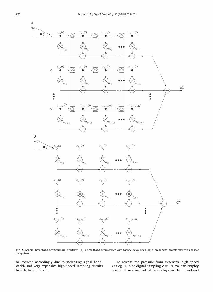
impulse response (FIR) filter to each of received signals in itsdiscrete form [4–6]. As shown in Fig. 2(a), each receivedsignal xmðtÞ, m ¼ 0;1; . . . ;M � 1 is processed by a followingTDL with an adjacent tap delay of D and a corresponding tapweight wm;j, m ¼ 0;1; . . . ;M � 1, j ¼ 0;1; . . . ; J � 1. This isthe well-known broadband beamforming structure with TDLprocessing.

Previous studies have found that the length of the TDL,J, is dependent on the bandwidth of the impinging signalsand the larger the bandwidth the more delay-line taps arerequired [7–9]. The delays between adjacent taps need to

xM−1(t) wM−1

Fig. 1. A general linear array structure.

ARTICLE IN PRESS

Fig. 2. General broadband beamforming structures. (a) A broadband beamformer with tapped delay-lines. (b) A broadband beamformer with sensor

delay-lines.

N. Lin et al. / Signal Processing 90 (2010) 269–281270

be reduced accordingly due to increasing signal band-width and very expensive high speed sampling circuitshave to be employed.

To release the pressure from expensive high speedanalog TDLs or digital sampling circuits, we can employsensor delays instead of tap delays in the broadband

ARTICLE IN PRESS

N. Lin et al. / Signal Processing 90 (2010) 269–281 271

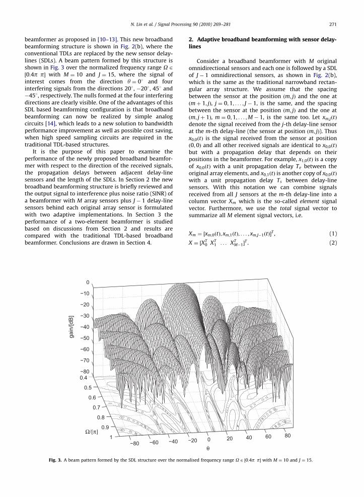
beamformer as proposed in [10–13]. This new broadbandbeamforming structure is shown in Fig. 2(b), where theconventional TDLs are replaced by the new sensor delay-lines (SDLs). A beam pattern formed by this structure isshown in Fig. 3 over the normalized frequency range O 2½0:4p p� with M ¼ 10 and J ¼ 15, where the signal ofinterest comes from the direction y ¼ 0� and fourinterfering signals from the directions 20�, �20�, 45� and�45�, respectively. The nulls formed at the four interferingdirections are clearly visible. One of the advantages of thisSDL based beamforming configuration is that broadbandbeamforming can now be realized by simple analogcircuits [14], which leads to a new solution to bandwidthperformance improvement as well as possible cost saving,when high speed sampling circuits are required in thetraditional TDL-based structures.

It is the purpose of this paper to examine theperformance of the newly proposed broadband beamfor-mer with respect to the direction of the received signals,the propagation delays between adjacent delay-linesensors and the length of the SDLs. In Section 2 the newbroadband beamforming structure is briefly reviewed andthe output signal to interference plus noise ratio (SINR) ofa beamformer with M array sensors plus J � 1 delay-linesensors behind each original array sensor is formulatedwith two adaptive implementations. In Section 3 theperformance of a two-element beamformer is studiedbased on discussions from Section 2 and results arecompared with the traditional TDL-based broadbandbeamformer. Conclusions are drawn in Section 4.

0.4

0.5

0.6

0.7

0.8

0.9

1−80 −60 −40

−80

−70

−60

−50

−40

−30

−20

−10

0

Ω/[π]

gain

/[dB

]

Fig. 3. A beam pattern formed by the SDL structure over the norm

2. Adaptive broadband beamforming with sensor delay-lines

Consider a broadband beamformer with M originalomnidirectional sensors and each one is followed by a SDLof J � 1 omnidirectional sensors, as shown in Fig. 2(b),which is the same as the traditional narrowband rectan-gular array structure. We assume that the spacingbetween the sensor at the position ðm; jÞ and the one atðmþ 1; jÞ, j ¼ 0;1; . . . ; J � 1, is the same, and the spacingbetween the sensor at the position ðm; jÞ and the one atðm; jþ 1Þ, m ¼ 0;1; . . . ;M � 1, is the same too. Let xm;jðtÞ

denote the signal received from the j-th delay-line sensorat the m-th delay-line (the sensor at position ðm; jÞ). Thusx0;0ðtÞ is the signal received from the sensor at positionð0;0Þ and all other received signals are identical to x0;0ðtÞ

but with a propagation delay that depends on theirpositions in the beamformer. For example, x1;0ðtÞ is a copyof x0;0ðtÞ with a unit propagation delay Te between theoriginal array elements, and x0;1ðtÞ is another copy of x0;0ðtÞ

with a unit propagation delay Ts between delay-linesensors. With this notation we can combine signalsreceived from all J sensors at the m-th delay-line into acolumn vector Xm which is the so-called element signalvector. Furthermore, we use the total signal vector tosummarize all M element signal vectors, i.e.

Xm ¼ ½xm;0ðtÞ; xm;1ðtÞ; . . . ; xm;J�1ðtÞ�T , (1)

X ¼ ½XT0 XT

1 . . . XTM�1�

T . (2)

−20 0 20 40 60 80

θ

alised frequency range O 2 ½0:4p p� with M ¼ 10 and J ¼ 15.

ARTICLE IN PRESS

N. Lin et al. / Signal Processing 90 (2010) 269–281272

Each sensor in the beamformer has a correspondingweight, and the beamformer output is formed as a linearcombination of the received sensor signals. We denote theweight attached to the ðm; jÞ-th sensor as wm;j, all J weightsat the m-th delay-line as an element weight vector Wm andall M element weight vectors as a total weight vector W,

Wm ¼ ½wm;0;wm;1; . . . ;wm;J�1�T , (3)

W ¼ ½WT0 WT

1 � � � WTM�1�

T . (4)

The conventional TDL based beamformer may applyadaptive algorithms to determine its weights to optimizethe beamformer response. These adaptive algorithms canbe easily extended to the SDL based beamformingstructure [13]. In this paper we take the reference signalbased as well as the linearly constrained adaptiveimplementations as two examples.

2.1. Reference signal based adaptive beamforming

In the reference signal based adaptive beamformer, areference signal rðtÞ is available and the weights areadjusted to minimize the mean square error (MSE)between the beamformer output yðtÞ and the referencerðtÞ, as shown in Fig. 4. The optimal weight vector in (4) isthen given by [4]

Wopt ¼ F�1x S, (5)

where Fx is the signal correlation matrix ðMJ �MJÞ,

Fx ¼ E½X�XT�, (6)

and S is the reference correlation vector ðMJ � 1Þ,

S ¼ E½X�r0ðtÞ�. (7)

The asterisk denotes the complex conjugate operation andr0ðtÞ is the normalized reference signal with unit power.

In this study we assume that the received signal ateach sensor consists of three uncorrelated components: adesired signal dðtÞ from yd, an interference iðtÞ from yi anda white noise signal nðtÞ. Thus the received signal at theðm; jÞ-th sensor can be expressed as

xm;jðtÞ ¼ dm;jðtÞ þ im;jðtÞ þ nm;jðtÞ, (8)

where dm;jðtÞ, im;jðtÞ and nm;jðtÞ are the assumed desiredsignal, interference and white noise components receivedat the ðm; jÞ-th sensor, respectively. We can then expressthe element signal vector Xm and total signal vector X as

−

y(t)

+r(t) e(t)

X(t) W

Fig. 4. Reference based adaptive beamforming structure.

Xm ¼ Xdmþ Xim þ Xnm (9)

and

X ¼ Xd þ Xi þ Xn. (10)

Finally the signal correlation matrix Fx can be decom-posed into three correlation matrices corresponding to thedesired signal, interference and white noise components,respectively, i.e.

Fx ¼ Fd þFi þFn. (11)

These three correlation matrices can be determined asfollows.

We consider Fd first. Assume the desired signal dðtÞ hasa flat power spectral density of 2ppd=Dod and a limitedbandwidth Dod centered at oo, as shown in Fig. 5. Itscorrelation function RdðtÞ can be obtained by the inverseFourier transform [7],

RdðtÞ ¼ pd sincDodt

2

� �eio0t, (12)

where pd is the desired signal average power at eachsensor and t is the delay. Now we can partition Fd intoM �M sub matrices

Fd ¼

Fd0;0Fd0;1

� � � Fd0;M�1

Fd1;0Fd1;1

� � � Fd1;M�1

..

. ... . .

. ...

FdM�1;1FdM�1;1

� � � FdM�1;M�1

0BBBBB@

1CCCCCA, (13)

where each sub matrix Fdm;n(J � J) is a desired signal

correlation matrix associated with the element signalvectors Xdm

and Xdn,

Fdm;n¼ E½X�dm

XTdn�. (14)

Note the ðj; kÞ-th element in Fdm;nis the correlation of the

desired signals received at the ðm; jÞ-th and the ðn; kÞ-thsensors. Note that the desired signal received at the sensorpositioned at ðp; qÞ is a copy of the original desired signaldðtÞ with a delay among the original array elements aswell as a delay among delay-line sensors, i.e.

dp;qðtÞ ¼ dðt � pTe � qTsÞ, (15)

where Te is the unit propagation delay between theoriginal adjacent array elements and Ts is the unitpropagation delay between adjacent delay-line sensors.Thus the correlation of the desired signal received at theðm; jÞ-th and the ðn; kÞ-th sensor is given by

ωωo

Sd

Δωd

2πPdΔωd

Fig. 5. Power spectral density of the desired signal.

ARTICLE IN PRESS

N. Lin et al. / Signal Processing 90 (2010) 269–281 273

½Fdm;n�j;k ¼ E½d�m;jðtÞdn;kðtÞ�

¼ Rd½ðm� nÞTe þ ðj� kÞTs�. (16)

To avoid spatial aliasing it is often assumed that twoadjacent array sensors are half a wavelength apart fromeach other at the maximum signal frequency, omax andthe unit propagation delay between the original arrayelements is therefore

Te ¼L

csinðydÞ ¼

pomax

sinðydÞ, (17)

where yd is the direction of arrival (DOA) of the desiredsignal, c is the signal propagation speed, and L is theelement spacing between the adjacent original arraysensors. To study the effect of delay between delay-linesensors we assume that the two adjacent delay-linesensors are r times a quarter wavelength apart from eachother at omax. The unit propagation delay between delay-line sensors is then

Ts ¼D

ccosðydÞ ¼

p2omax

r cosðydÞ, (18)

where D is the spacing between adjacent SDL sensors.Substituting (12) into (16) we now have

½Fdm;n�j;k ¼ pd sinc

Dod

2½ðm� nÞTe þ ðj� kÞTs�

� ��eioo½ðm�nÞTeþðj�kÞTs �. (19)

To simplify the above equation we can replace theabsolute bandwidth and center frequency with theirrelative counterparts Bd ¼ Dod=omax and Oo ¼ oo=omax,respectively. Therefore the terms DodTe and ooTe can bewritten as

DodTe ¼Dod

omaxp sinðydÞ ¼ Bdp sinðydÞ (20)

and

ooTe ¼oo

omaxp sinðydÞ ¼ Oop sinðydÞ. (21)

Similarly, we have

DodTs ¼Dod

omax

p2

r cosðydÞ ¼ Bdp2

r cosðydÞ, (22)

and

ooTs ¼oo

omax

p2

r cosðydÞ ¼ Oop2

r cosðydÞ. (23)

We can now give the full expression for the autocorrela-tion of the desired signal at the ðm; jÞ-th sensor and theðn; kÞ-th sensor in its simplified form,

½Fdm;n�j;k ¼ pd sinc

Bd

2td

� �eiOotd , (24)

where the delay td is expressed as

td ¼ p ðm� nÞ sinðydÞ þ ðj� kÞr

2cosðydÞ

h i. (25)

The interference correlation matrix Fi in (11) can bedetermined in the same way. Again we shall assume theinterference iðtÞ has a flat power spectral density of2ppi=Doi and a limited bandwidth Doi centered at oo.Therefore Fi can be found as

Fi ¼

Fi0;0 Fi0;1 � � � Fi0;M�1

Fi1;0 Fi1;1 � � � Fi1;M�1

..

. ... . .

. ...

FiM�1;1FiM�1;1

� � � FiM�1;M�1

0BBBBB@

1CCCCCA, (26)

where each ðj; kÞ-th term in each M �M sub matrix Fim;n

ðJ � JÞ is the autocorrelation of the interference at theðm; jÞ-th and ðn; kÞ-th sensors and can be expressed as

½Fim;n �j;k ¼ pi sincBi

2ti

� �eiOoti , (27)

where Bi is defined in the same way as Bd and

ti ¼ p ðm� nÞ sinðyiÞ þ ðj� kÞr

2cosðyiÞ

h i. (28)

The noise correlation matrix Fn is different from the othertwo. Each sensor in the beamformer is an independentanalog device and therefore the noise signals are un-correlated with each other. By assuming the noisevariance to be s2 the noise correlation matrix is given by

Fn ¼ s2

1 0 � � � 0

0 1 � � � 0

..

. ... . .

. ...

0 0 � � � 1

0BBBB@

1CCCCA ¼ s2I, (29)

where I is an identity matrix with size MJ �MJ.Now we give the reference correlation vector S in (7).

Assume that the reference signal is the same as thedesired signal. As discussed before the desired signal,interference and noise vectors are uncorrelated with eachother. Thus the only term in S is Xd,

S ¼ E½X�doðtÞ� ¼ E½X�ddoðtÞ�, (30)

where doðtÞ is identical to dðtÞ but with a unit power.In the same way we can express S as

S ¼ ½s0;0; s0;1; . . . ; s0;J�1; . . . ; sM�1;0; sM�1;1; . . . ; sM�1;J�1�T ,

(31)

and each ðm; jÞ-th term in S is the correlation of the desiredsignal at the ðm; jÞ-th sensor and the reference signal itself,

sm;j ¼ffiffiffiffiffipd

psinc

Bd

2ts

� �eiOots , (32)

where

ts ¼ p m sinðydÞ þ jr

2cosðydÞ

h i. (33)

The relative bandwidth Bd and the relative centerfrequency Oo are defined as before. Now with fullydefined Fx and S the optimal weight vector Wopt can bedetermined from (5).

Then the beamformer output yðtÞ is

yðtÞ ¼WToptX, (34)

with its power given by

P ¼1

2E½kyðtÞk2�

¼1

2WH

optFxWopt , (35)

where f�gH denotes the Hermitian transpose. Since Fx can

ARTICLE IN PRESS

N. Lin et al. / Signal Processing 90 (2010) 269–281274

be expressed as the sum of three individual terms in (11),the output power can also be expressed as the sum ofthree corresponding components, named as output de-sired signal power, output interference power and outputnoise power,

Pd ¼WHoptFdWopt , (36)

Pi ¼WHoptFiWopt , (37)

Pn ¼WHoptFnWopt . (38)

The output SINR is then given by

SINR ¼Pd

Pi þ Pn. (39)

2.2. Linearly constrained adaptive beamforming

In practice, the reference signal rðtÞ assumed in Section2.1 is not always available. However, some information onthe DOAs as well as the bandwidth limits of the desiredsignal and/or the interferences could be available. In thiscase Frost suggested a linearly constrained minimumvariance (LCMV) beamformer [15] which imposes someconstraints on the beamformer weights so that signalsfrom desired directions can pass with specified responsewhile contributions to the output variance (or power) dueto interferences from directions other than the desiredones are minimized. The LCMV beamformer structure isshown in Fig. 6 and the problem can be formulated as

minW

WHFxW subject to CHW ¼ f , (40)

where W and Fx are defined before in Section 2.1, C is theconstraint matrix and f is the response vector. Eq. (40)implies that with the constraint matrix C the LCMVbeamformer will always have the desired response set outby the constraint equation CHW ¼ f no matter how theweights are adjusted. The solution to (40) can be obtainedusing the Lagrange multipliers method [15],

Wopt ¼ F�1x CðCHF�1

x C�1f . (41)

Fx is defined in the same way as in Section 2.1 and the

y(t)

CHW = f

X(t) W

Fig. 6. The LCMV beamforming structure.

x0 (t) x1 (t)

w0 w1

x (t)

Fig. 7. Equivalent beamformer wit

constraint matrix C and response vector f are determinedas follows.

Suppose the signal of interest comes from yd ¼ 0�.Then, for the desired signal, identical signal componentsappear at the array elements simultaneously. Thus theattached SDLs appear to be driven by a common input andthe beamformer can be seen as a single sensor delay-linein which each weight is the sum of the weights in thecorresponding column as shown in Fig. 7. For a distortion-less response to the desired signal, the beamformerresponse is a pure time delay where only one of thecoefficients in Fig. 7 is one and all the others are zero. Thusthe constraint matrix C can be written as M identitymatrices IJ (J � J),

C ¼ ½IJ � � � IJ �|fflfflfflfflfflffl{zfflfflfflfflfflffl}M

T , (42)

and the response vector f should only implement a delayas follows:

f ¼ ½0 � � � 1 � � � 0�|fflfflfflfflfflfflfflfflfflfflfflfflfflffl{zfflfflfflfflfflfflfflfflfflfflfflfflfflffl}J

T . (43)

In our simulations we choose the first element of f to beone.

With C and f determined the optimal weights vectorand consequently the output SINR can be obtained asshown previously in Section 2.1.

3. Performance of a two-element beamformer with SDLs

To examine the performance of the SDL basedbeamformer we now consider a simple two-element ðM ¼2Þ broadband beamformer receiving a desired signal fromthe broadside ðyd ¼ 0Þ and an arbitrary interference fromyi. We shall assume that both the desired signal and theinterference have the same bandwidth as well as thecenter frequency oo ¼ p=2. Moreover, the input SIR andSNR are assumed to be �20 and 20 dB, respectively.

In the discrete form the conventional TDL applies anFIR filter with a constant sampling period to each receivedsensor signal. However, as indicated in Eq. (18) the SDLnow introduces an ‘FIR filter’ with a sampling periodessentially depending on the DOA of the impinging signalfor a given r. To understand the effect of yi on thebandwidth performance we shall examine the transferfunction of a two-element beamformer fed with theinterference only. The transfer function of the m-th SDLwith J � 1 delay-line sensors is

HmðoÞ ¼ wm;0 þwm;1e�ioTs þ � � � þwm;J�1e�iðJ�1ÞoTs , (44)

x2 (t)

w2

xJ−1 (t)

wJ−1y(t)

h a single sensor delay-line.

ARTICLE IN PRESS

N. Lin et al. / Signal Processing 90 (2010) 269–281 275

and the transfer function for the whole two-elementbeamformer is

HðoÞ ¼ H0ðoÞ þ H1ðoÞe�ioTe , (45)

0 10 20 30 40−25

−20

−15

−10

−5

0

5

10

15

20

25S

INR

(dB

)

θi (d

Fig. 8. Beamformer output SINR versus

0 10 20 30 40−25

−20

−15

−10

−5

0

5

10

15

20

SIN

R (d

B)

0 10 20 30 40−25

−20

−15

−10

−5

0

5

10

15

20

SIN

R (d

B)

θi (d

θi (d

Fig. 9. SDL beamformer output SINR versus yi : M ¼ 2; J ¼ 2; r ¼ 1

where Te and Ts are defined in (17) and (18), respectively,but with yd being replaced by yi. In order to null theinterference completely HðoÞmust be zero over the wholesignal bandwidth,

50 60 70 80 90

B = 0.0B = 0.2B = 0.4B = 0.6B = 0.8

egree)

yi (reference based): M ¼ 2, J ¼ 1.

50 60 70 80 90

B = 0.2B = 0.4B = 0.6B = 0.8

50 60 70 80 90

B = 0.2B = 0.4B = 0.6B = 0.8

egree)

egree)

. (a) Reference based beamforming. (b) LCMV beamforming.

ARTICLE IN PRESS

N. Lin et al. / Signal Processing 90 (2010) 269–281276

H0ðoÞ ¼ �H1ðoÞe�ioTe . (46)

To meet (46) it is essential to ensure that H0ðoÞ and H1ðoÞhave the identical amplitude response and a phase shiftvarying linearly with frequency over the signal band-width, i.e.

kH0ðoÞk ¼ kH1ðoÞk (47)

and

ffH0ðoÞ ¼ ffH1ðoÞ � p�oTe. (48)

In a narrowband beamformer ðJ ¼ 1Þ, there are no delay-line sensors attached and only one weight is applied toeach received sensor signal. Therefore (46) becomes

w0;0 ¼ �w1;0e�ioTs , (49)

which can only be satisfied at a single frequency (B ¼ 0with B defined in the same way as Bd and Bi). As shown inFig. 8 for the reference signal based beamformer, largerbandwidth rapidly worsens the output SINR. A verysimilar result is obtained for the LCMV case. In contrast,with one single delay-line sensor ðJ ¼ 2Þ attached to eacharray sensor, HmðoÞ is then

HmðoÞ ¼ wm;0 þwm;1e�ioTs . (50)

10 20 30 41−15

−10

−5

0

5

10

15

20

SIN

R (d

B) r = 23

r = 12

r = 8

r = 6

10 20 30 41−15

−10

−5

0

5

10

15

SIN

R (d

B)

r = 23

r = 12

r = 8

r = 6

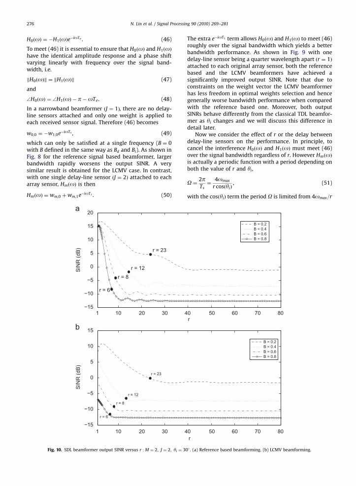
Fig. 10. SDL beamformer output SINR versus r : M ¼ 2; J ¼ 2; yi ¼ 3

The extra e�ioTs term allows H0ðoÞ and H1ðoÞ to meet (46)roughly over the signal bandwidth which yields a betterbandwidth performance. As shown in Fig. 9 with onedelay-line sensor being a quarter wavelength apart ðr ¼ 1Þattached to each original array sensor, both the referencebased and the LCMV beamformers have achieved asignificantly improved output SINR. Note that due toconstraints on the weight vector the LCMV beamformerhas less freedom in optimal weights selection and hencegenerally worse bandwidth performance when comparedwith the reference based one. Moreover, both outputSINRs behave differently from the classical TDL beamfor-mer as yi changes and we will discuss this difference indetail later.

Now we consider the effect of r or the delay betweendelay-line sensors on the performance. In principle, tocancel the interference H0ðoÞ and H1ðoÞ must meet (46)over the signal bandwidth regardless of r. However HmðoÞis actually a periodic function with a period depending onboth the value of r and yi,

O ¼2pTs¼

4omax

r cosðyiÞ, (51)

with the cosðyiÞ term the period O is limited from 4omax=r

0 50 60 70 80r

B = 0.2B = 0.4B = 0.6B = 0.8

0 50 60 70 80r

B = 0.2B = 0.4B = 0.6B = 0.8

0� . (a) Reference based beamforming. (b) LCMV beamforming.

ARTICLE IN PRESS

N. Lin et al. / Signal Processing 90 (2010) 269–281 277

to þ1. For large r values the lower bound of O is muchsmaller than the signal bandwidth. But the lower boundwill increase as r decreases and it will finally equal to thesignal bandwidth when

r ¼4

B cosðyiÞ. (52)

If r is very small, 4omax=r is large and O is always muchlarger than the signal bandwidth. Therefore the phaseshift ffH0ðoÞ � ffH1ðoÞ can be linear and in this case it ispossible to meet the requirement in Eq. (46) and have agood performance. As r increases the lower bound of Oapproaches the signal bandwidth and it becomes moredifficult for H0ðoÞ and H1ðoÞ to satisfy (46) within thesignal bandwidth and the beamformer performancedrops. When r exceeds its critical value 4=ðB cosðyiÞÞ,4omax=r eventually drops below the signal bandwidth andffH0ðoÞ � ffH1ðoÞ may repeat periodically within thesignal bandwidth (depending on the value of yi) therefore(46) cannot be met any more. At this point there will belittle change to a poor bandwidth performance with larger values. The above discussions are illustrated in Fig. 10and the corresponding critical value of r ¼ 4=ðB cosðyiÞÞ, is

0 10 20 30 40−25

−20

−15

−10

−5

0

5

10

15

20

SIN

R (d

B)

r = 35 and 80

0 10 20 30 40−25

−20

−15

−10

−5

0

5

10

15

20

25

SIN

R (d

B)

θi (d

θi (de

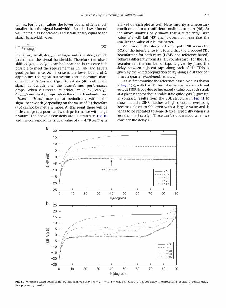
Fig. 11. Reference based beamformer output SINR versus yi : M ¼ 2; J ¼ 2; B ¼

line processing results.

marked on each plot as well. Note linearity is a necessarycondition and not a sufficient condition to meet (46). Sothe above analysis only shows that a sufficiently largevalue of r will fail (46) and it does not mean that thesmaller the value of r is, the better.

Moreover, in the study of the output SINR versus theDOA of the interference it is found that the proposed SDLbeamformer, for both cases (LCMV and reference based),behaves differently from its TDL counterpart. (For the TDLbeamformer, the number of taps is given by J and thedelay between adjacent taps along each of the TDLs isgiven by the wired propagation delay along a distance of r

times a quarter wavelength at omax.)Let us first examine the reference based case. As shown

in Fig. 11(a), with the TDL beamformer the reference basedoutput SINR drops due to increased r value but each resultat a given r approaches a stable state quickly as yi goes up.In contrast, results from the SDL structure in Fig. 11(b)show that the SINR reaches a high constant level as yi

becomes closer to 90� even with a large r value and ittends to be repeated to some degree, especially when r isless than 4=ðB cosðyiÞÞ. These can be understood when weconsider the delay ti.

50 60 70 80 90

r = 5r = 15r = 25r = 35r = 80

50 60 70 80 90

r = 5r = 15r = 25r = 35r = 80

egree)

gree)

0:2; r 2 ð5;80Þ. (a) Tapped delay-line processing results. (b) Sensor delay-

ARTICLE IN PRESS

N. Lin et al. / Signal Processing 90 (2010) 269–281278

From (18) it is clear that as yi ! 90� Ts approaches 0and the SDL structure fails to null the broadbandinterference. On the contrary, Te in (17) increasessignificantly regardless of r as Ts falls. Due to increasedpropagation delay between the original array elements,the correlation of the interference within the wholebeamformer is restored and the beamformer is still ableto cancel the interference even without the help of SDL atlarge yi values. Also, from the trigonometric identities, ti

can be rewritten as

ti ¼ p

ffiffiffiffiffiffiffiffiffiffiffiffiffiffiffiffiffiffiffiffiffiffiffiffiffiffiffiffiffiffiffiffiffiffiffiffiffiffiffiffiffiffiffiffiffiffiffiðm� nÞ2 þ

ðj� kÞr

2

� 2s

sinðyi þ ciÞ, (53)

where

ci ¼ tan�1 ðj� kÞr

ðm� nÞ2

� . (54)

This is a periodic function with a complicated perioddepending on the position of the sensor, yi and r. Thus theoutput SINR will behave periodically to some degree.

Now let us discuss the LCMV case. Again, with theconventional TDL structure, the LCMV beamformer result

0 10 20 30 40−25

−20

−15

−10

−5

0

SIN

R (d

B)

r = 35 an

0 10 20 30 40−25

−20

−15

−10

−5

0

5

10

15

SIN

R (d

B)

θi (d

θi (d

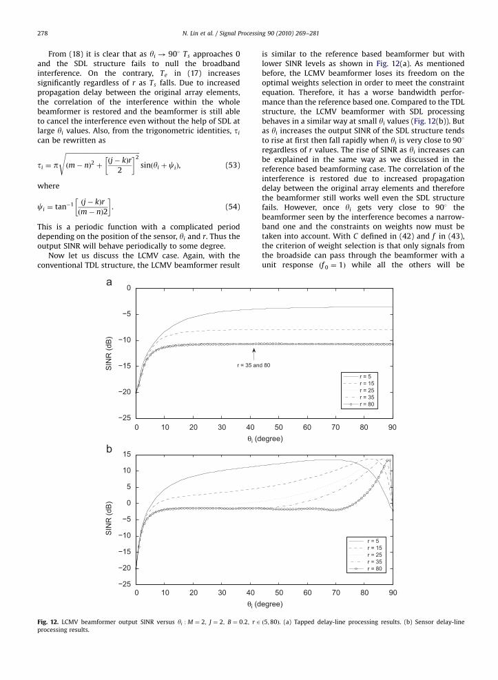
Fig. 12. LCMV beamformer output SINR versus yi : M ¼ 2; J ¼ 2; B ¼ 0:2; r 2

processing results.

is similar to the reference based beamformer but withlower SINR levels as shown in Fig. 12(a). As mentionedbefore, the LCMV beamformer loses its freedom on theoptimal weights selection in order to meet the constraintequation. Therefore, it has a worse bandwidth perfor-mance than the reference based one. Compared to the TDLstructure, the LCMV beamformer with SDL processingbehaves in a similar way at small yi values (Fig. 12(b)). Butas yi increases the output SINR of the SDL structure tendsto rise at first then fall rapidly when yi is very close to 90�

regardless of r values. The rise of SINR as yi increases canbe explained in the same way as we discussed in thereference based beamforming case. The correlation of theinterference is restored due to increased propagationdelay between the original array elements and thereforethe beamformer still works well even the SDL structurefails. However, once yi gets very close to 90� thebeamformer seen by the interference becomes a narrow-band one and the constraints on weights now must betaken into account. With C defined in (42) and f in (43),the criterion of weight selection is that only signals fromthe broadside can pass through the beamformer with aunit response ðf 0 ¼ 1Þ while all the others will be

50 60 70 80 90

r = 5r = 15r = 25r = 35r = 80

d 80

50 60 70 80 90

r = 5r = 15r = 25r = 35r = 80

egree)

egree)

ð5;80Þ. (a) Tapped delay-line processing results. (b) Sensor delay-line

ARTICLE IN PRESS

N. Lin et al. / Signal Processing 90 (2010) 269–281 279

attenuated, i.e.

w0;0 þw1;0 ¼ 1;

w0;1 þw1;1 ¼ 0:

((55)

When the broadband beamformer seen by the interfer-ence approximates a narrowband one as yi ! 90�, eachweight of the equivalent narrowband beamformer is thesum of weights in the corresponding delay-line, i.e.

w0 ¼ w0;0 þw0;1;

w1 ¼ w1;0 þw1;1:

((56)

Since they must follow the constraint on optimal weightsselection as well, we have

w0 þw1 ¼ 1. (57)

Therefore the performance drops to the level of thecorresponding narrowband LCMV beamformer. We alsonote that unlike the reference based beamformer in theLCMV case there is no repetition in the output SINR, whichis another effect due to the constraint on weight selection.The ti in (53) is periodic to some degree only and the

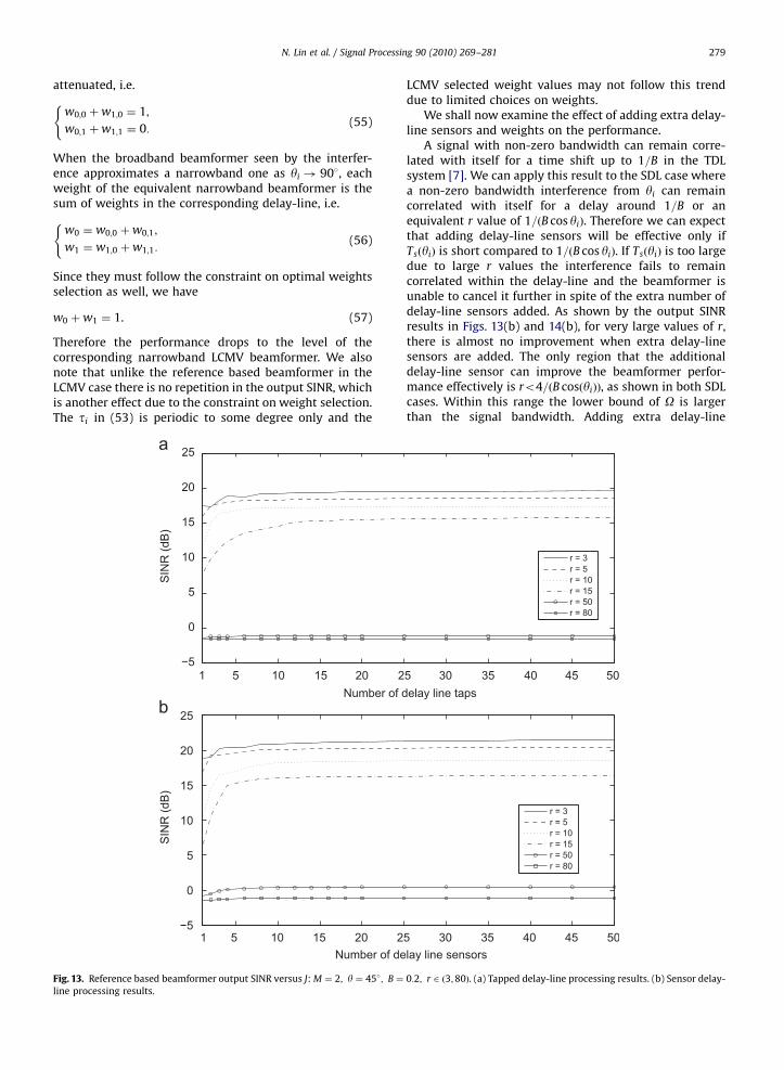
Fig. 13. Reference based beamformer output SINR versus J: M ¼ 2; y ¼ 45�; B ¼

line processing results.

LCMV selected weight values may not follow this trenddue to limited choices on weights.

We shall now examine the effect of adding extra delay-line sensors and weights on the performance.

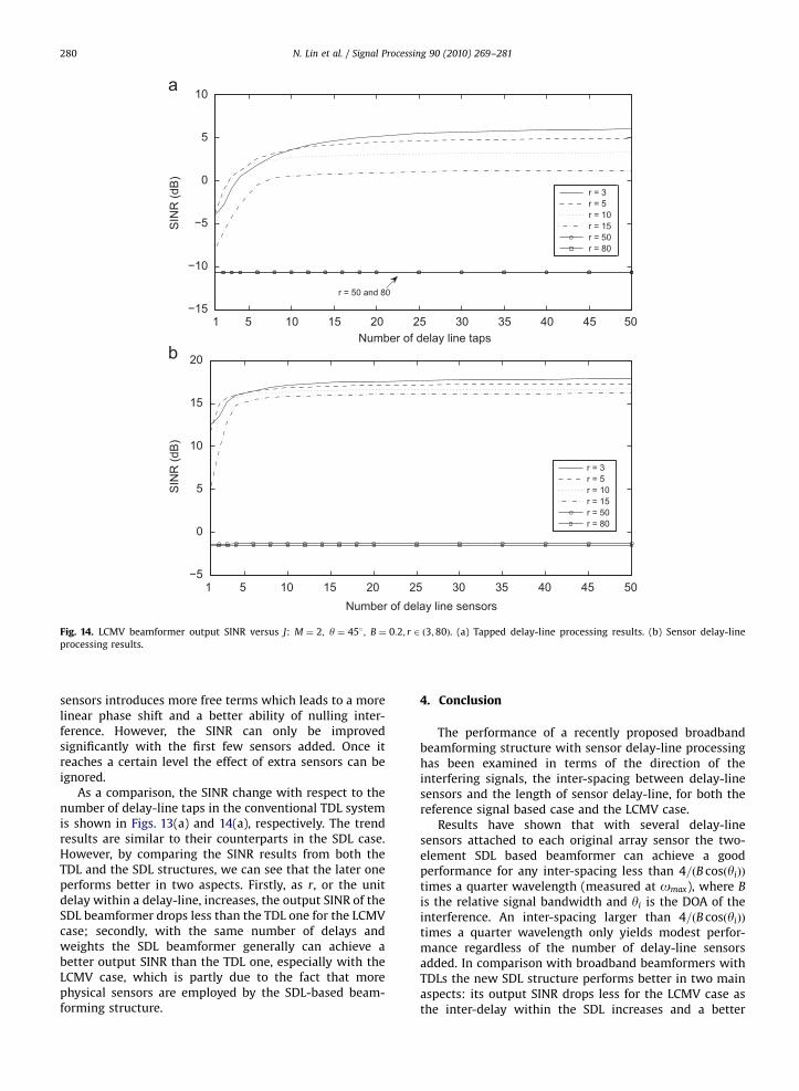
A signal with non-zero bandwidth can remain corre-lated with itself for a time shift up to 1=B in the TDLsystem [7]. We can apply this result to the SDL case wherea non-zero bandwidth interference from yi can remaincorrelated with itself for a delay around 1=B or anequivalent r value of 1=ðB cos yiÞ. Therefore we can expectthat adding delay-line sensors will be effective only ifTsðyiÞ is short compared to 1=ðB cos yiÞ. If TsðyiÞ is too largedue to large r values the interference fails to remaincorrelated within the delay-line and the beamformer isunable to cancel it further in spite of the extra number ofdelay-line sensors added. As shown by the output SINRresults in Figs. 13(b) and 14(b), for very large values of r,there is almost no improvement when extra delay-linesensors are added. The only region that the additionaldelay-line sensor can improve the beamformer perfor-mance effectively is ro4=ðB cosðyiÞÞ, as shown in both SDLcases. Within this range the lower bound of O is largerthan the signal bandwidth. Adding extra delay-line

0:2; r 2 ð3;80Þ. (a) Tapped delay-line processing results. (b) Sensor delay-

ARTICLE IN PRESS

5 10 15 20 25 30 35 40 45 501−15

−10

−5

0

5

10

Number of delay line taps

SIN

R (d

B)

r = 3r = 5r = 10r = 15r = 50r = 80

r = 50 and 80

5 10 15 20 25 30 35 40 45 501−5

0

5

10

15

20

Number of delay line sensors

SIN

R (d

B)

r = 3r = 5r = 10r = 15r = 50r = 80

Fig. 14. LCMV beamformer output SINR versus J: M ¼ 2; y ¼ 45� ; B ¼ 0:2; r 2 ð3;80Þ. (a) Tapped delay-line processing results. (b) Sensor delay-line

processing results.

N. Lin et al. / Signal Processing 90 (2010) 269–281280

sensors introduces more free terms which leads to a morelinear phase shift and a better ability of nulling inter-ference. However, the SINR can only be improvedsignificantly with the first few sensors added. Once itreaches a certain level the effect of extra sensors can beignored.

As a comparison, the SINR change with respect to thenumber of delay-line taps in the conventional TDL systemis shown in Figs. 13(a) and 14(a), respectively. The trendresults are similar to their counterparts in the SDL case.However, by comparing the SINR results from both theTDL and the SDL structures, we can see that the later oneperforms better in two aspects. Firstly, as r, or the unitdelay within a delay-line, increases, the output SINR of theSDL beamformer drops less than the TDL one for the LCMVcase; secondly, with the same number of delays andweights the SDL beamformer generally can achieve abetter output SINR than the TDL one, especially with theLCMV case, which is partly due to the fact that morephysical sensors are employed by the SDL-based beam-forming structure.

4. Conclusion

The performance of a recently proposed broadbandbeamforming structure with sensor delay-line processinghas been examined in terms of the direction of theinterfering signals, the inter-spacing between delay-linesensors and the length of sensor delay-line, for both thereference signal based case and the LCMV case.

Results have shown that with several delay-linesensors attached to each original array sensor the two-element SDL based beamformer can achieve a goodperformance for any inter-spacing less than 4=ðB cosðyiÞÞ

times a quarter wavelength (measured at omax), where B

is the relative signal bandwidth and yi is the DOA of theinterference. An inter-spacing larger than 4=ðB cosðyiÞÞ

times a quarter wavelength only yields modest perfor-mance regardless of the number of delay-line sensorsadded. In comparison with broadband beamformers withTDLs the new SDL structure performs better in two mainaspects: its output SINR drops less for the LCMV case asthe inter-delay within the SDL increases and a better

ARTICLE IN PRESS

N. Lin et al. / Signal Processing 90 (2010) 269–281 281

output SINR can be archived using the same number ofdelays as the TDL one.

In addition, it has also been found that the SDLbeamformer behaves differently from each other withrespect to the DOA of the interfering signals. In thereference based implementation the SINR increases as yi

gets close to 90� for all inter-spacing values. On thecontrary the output SINR in the LCMV implementationtends to increase when yi ! 90� at first but suddenlydrops to a narrowband level if yi is very close to 90� due tothe constraint on optimal weights selection.

References

[1] H.L. Van Trees, Optimum Array Processing, Part IV of Detection,Estimation, and Modulation Theory, Wiley, New York, USA, 2002.

[2] R.A. Monzingo, T.W. Miller, Introduction to Adaptive Arrays, SciTechPublishing Inc., USA, 2004.

[3] B. Allen, M. Ghavami, Adaptive Array Systems, Fundamentals andApplications, Wiley, New York, 2005.

[4] B. Widrow, P.E. Mantey, L.J. Griffiths, B.B. Goode, Adaptive antennasystems, Proceedings of the IEEE 55 (December 1967) 2143–2159.

[5] W.E. Rodgers, R.T. Compton Jr., Adaptive array bandwidth withtapped delay-line processing, IEEE Transactions on AerospaceElectronic Systems AES-15 (1) (1979) 21–27.

[6] J.T. Mayhan, A.J. Simmons, W.C. Cummings, Wide-bandadaptive antenna nulling using tapped delay lines, IEEE Transac-

tions on Antennas and Propagation AP-29 (November 1981)923–936.

[7] R.T. Compton, The bandwidth performance of a two-elementadaptive array with tapped delay-line processing, IEEE Transactionson Antennas and Propagation 36 (1) (January 1988) 4–14.

[8] E.W. Vook, R.T. Compton Jr., Bandwidth performance of linearadaptive arrays with tapped delay-line processing, IEEE Transac-tions on Aerospace and Electronic Systems 28 (3) (July 1992)901–908.

[9] L. Yu, N. Lin, W. Liu, R. Langley, Bandwidth performance of linearlyconstrained minimum variance beamformers, in: Proceedings of theIEEE International Workshop on Antenna Technology, Cambridge,UK, March 2007, pp. 327–330.

[10] W. Liu, Adaptive broadband beamforming with spatial-onlyinformation, in: Proceedings of the International Conference onDigital Signal Processing, Cardiff, UK, July 2007, pp. 575–578.

[11] W. Liu, D. McLernon, M. Ghogho, Frequency invariant beamformingwithout tapped delay-lines, in: Proceedings of the IEEE Interna-tional Conference on Acoustics, Speech, and Signal Processing,Hawaii, US, vol. 2, April 2007, pp. 997–1000.

[12] W. Liu, S. Weiss, Broadband beamspace adaptive beamforming withspatial-only information, in: Proceedings of the IEEE Workshop onSensor Array and Multichannel Signal Processing, Darmstadt,Germany, July 2008, pp. 330–334.

[13] W. Liu, Adaptive wideband beamforming with sensor delay-lines,Signal Processing 89 (May 2009) 876–882.

[14] A. Carusone, D.A. Johns, Analogue adaptive filters: past and present,IEE Proceedings—Circuits, Devices and Systems 147 (1) (February2000) 82–90.

[15] O.L. Frost III, An algorithm for linearly constrained adaptivearray processing, Proceedings of the IEEE 60 (8) (August 1972)926–935.