1

Abstract— Wireless mesh networks are the next step in the

evolution of wireless architecture, delivering wireless

services for a large variety of applications in personal,

local, campus, and metropolitan area. Ad hoc wireless

networks are increasingly gaining importance due to

their advantages such as low cost and ease of

deployment .In this paper, we present a detailed simulation

study of the performance of different routing algorithms

like Adhoc On demand Distance Vector Routing(AODV),

Destination Sequenced Distance Vectored routing,

Dynamic Source routing, Dumb Agent Protocol in ad hoc

and wireless mesh networks using ns2(Network simulator)

environment. We also implement hardware configuration

of the mesh routers.

Index Terms— Adhoc, Wireless mesh networks, Network

simulator(ns-2), DSDV, AODV, DSR, TCL, Cygwin

I. INTRODUCTION

Wireless networking is an emerging technology that allows users to access information and services electronically, regardless of their geographic position. Wireless networks can be classified in two types namely Infrastructure Networks and Infrastructure less Networks. Infrastructure Network:

Infrastructure network consists of a network with fixed and wired gateways. A mobile host communicates with a bridge in the network (called base station) within its communication radius. The mobile unit can move geographically while it is communicating. In addition to acting as a router within the network, an access point can also act as a bridge connecting, for example, the wireless network to a wired network. GSM, and its 3G counterpart UMTS, are examples of well known cellular networks. When it goes out of range of one base station, it connects with new base station and starts communicating through it. This is called handoff.

Infrastructure less:

Ad Hoc Network is a collection of mobile nodes forming short live or temporary networks without the aid of any centralized

structure. All nodes are capable of movement and are connected dynamically. In this type of network there is no base station that acts as a router, instead each node functions as a router, forwarding data for other nodes. Due to the recent advancements and commercial growth in wireless communication technology, MANET is expected to be very useful for the deployment of temporary networks in emergency situations such as fire, safety, rescue operations, meetings or conventions in which persons wish to quickly share information, and data acquisition operations using autonomous vehicles. The main challenge of MANET is that the connections between the nodes within the network are continuously changing. Thus routing protocols must be adaptive and fast enough to maintain routes in spite of the changing network topology. In this approach the base stations are fixed. An ad hoc network is characterized by its fully distributed control mechanisms and self-organized behavior. Such a network is expected to work in the absence of any infrastructure by autonomously creating multihop paths for packet delivery. A wireless mesh network, as a variant of Mobile Ad hoc Networks (MANET), is an IEEE 802.11-based infrastructure network in which Access Points (APs) and stations (STA or hosts) can relay messages on behalf of other APs in ad hoc fashion to create a self-configuring system that extends the coverage range and increases the available bandwidth. The Ad hoc On Demand Distance Vector (AODV) routing algorithm is a routing protocol designed for ad hoc mobile networks. AODV builds routes using a route request / route reply query cycle. When a source node desires a route to a destination for which it does not already have a route, it broadcasts a route request (RREQ) packet across the network. The Dynamic Source Routing (DSR) is developed for mobile ad hoc networks. DSR protocol adapts quickly to routing changes when host movement is at a higher rate, yet requires little or no overhead during periods in which hosts move less frequently. In DSDV, routing messages are exchanged between neighboring mobile nodes (i.e. mobile nodes that are within range of one another). Dumb Agents routing, run no programs of their own, they simply host agents and provide a place to store a database of routing information. The mobile agents embody the “intelligence” in the system, moving from node to node and updating routing information as they go. Routing updates may be triggered or routine. Updates are triggered in case a routing information from one of t he neighbors forces a change in the routing table. A packet for which the route to its destination is not known is cached while routing queries are sent out. Based on results from a

Performance analysis of Routing protocols in wireless mesh and ad hoc networks

Sureshbabu Ramalingam, Subramanian Srinivasan, Lakshmikanth Yerradoddi

2

packet-level simulation of mobile hosts operating in an ad hoc network, the protocol performs well over a variety of environmental conditions such as host density and movement rates. In this paper, we evaluate the performance of these two algorithms in a wireless mesh network and in a ad-hoc network by streaming voice and video. Simulation Environment: Network simulator 2 (NS-2) is an open source discrete event simulation tool used for simulating Internet protocol (IP) networks. It was developed by UC Berkeley and widely used worldwide for network simulation purposes. The NS-2 software uses TCL as a front-end interpreter and C++ as the back end network simulation engine. Network simulation scripts in TCL are used to create the network scenarios and upon the completion of the simulation, trace files that capture events occurring in the network are produced. The trace files would capture information that could be used in performance study, e.g. the amount of packets transferred from source to destination, the delay in packets, packet loss etc. However, the trace file is just a block of ASCII data in a file and quite cumbersome to access using some form of post processing technique. The systems we used for simulation were based on windows operating system, but ns2 is a linux based application, hence we used cygwin to create linux like environment in windows. Cygwin is an open source collection of tools that allows Unix or Linux applications to be compiled and run on a Windows operating system from within a Linux-like interface. In this section, we discuss the research done on the mesh networks and mesh routers. In a traditional network, routers are used to direct data traffic from one place, or node, to another. Each router has a specific set of locations from which it can accept data, and a specific set of locations to which it can send data. A mesh network is a highly decentralized way of organizing nodes that does not require predetermined paths between them. Mesh routers work by continuously monitoring network activity and maintaining lists of other devices in their vicinity. When a potential node appears, it broadcasts its address and networking capabilities. Nearby mesh routers will receive the broadcast, and adjust their own lists to reflect the new node. When the device turns off or otherwise disappears, the mesh routers will again update their lists. One of the main challenges faced by mesh routers is security: because mesh routers automatically talk to every device that appears, it can be easier for unauthenticated users to gain access to the network. Another drawback of such networks is that without predetermined routing paths, data may take a longer time to reach its destination. Wireless routers contain built-in programmable logic called firmware. The firmware is embedded software that implements network and security protocols for a hardware device. Firmware is upgraded by downloading a binary file package from the manufacturer’s (Netgear) Web site. The router runs OpenWrt, a free Open Source Linux distribution for wireless routers. In fact, a low-

end wireless router is a small computer, which includes a CPU, and RAM and flash memory.

It is easily customized by replacing its original firmware by OpenWrt, a free Linux distribution for wireless routers, which is available since 2004 (http://openwrt.org). OpenWrt supports a large set of routers, and as an operating system, it is provided with the TCP/IP stack for networking.OpenWRT is one of the key drivers behind the Wi-Fi revolution. It got its start as an embedded Linux platform for wireless routers. It is an open source project to create a free embedded operating system for network devices. It mainly targeted wireless embedded hardware; OpenWrt has full support of wireless hardware and software. Software Installed: Ns2, Active Tcl scripts, Trace file generator, cygwin, network animator,Java.

II. INSTALLATIONS

Cygwin:

Installation steps for cygwin are as follows: 1. Download the setup.exe from www.cygwin.com.

Click this file. The below window will appear. Click “Next”.

3

2. Then choose “Install from Local Directory” option

and click “Next”.

3. Browse the root install directory and choose the default setting as follows:

4. Browse the Local package directory and click “Next”.

5. You will see the following progress window.

6. Select the required packages for your application from the list shown below. Generally make, patch, perl, gcc, gcc-g++, gawk, gnuplot, tar and gzip are basic packages required for ns2 simulations.

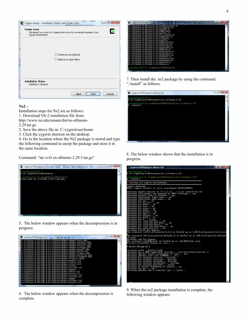
7. When the installation is completed, the following window will be shown. Select the create icon on Desktop and Add icon to Start Menu option and Click “Finish”.

4

Ns2 : Installation steps for Ns2 are as follows: 1. Download NS-2 installation file from: http://www.isi.edu/nsnam/dist/ns-allinone- 2.29.tar.gz 2. Save the above file in: C:\cygwin\usr\home 3. Click the cygwin shortcut on the desktop. 4. Go to the location where the Ns2 package is stored and type the following command to unzip the package and store it in the same location. Command: “tar xvfz ns-allinone-2.29.3.tar.gz”

5. The below window appears when the decompression is in progress.

6. The below window appears when the decompression is complete.

7. Then install the ns2 package by using the command “./install” as follows.

8. The below window shows that the installation is in progress.

9. When the ns2 package installation is complete, the following window appears.

5

III. ROUTING PROTOCOLS

Routing protocols can be divided into two categories:

• Table-Driven Routing Protocols

• On-Demand Routing Protocols Table-Driven Routing Protocols:

In table driven routing protocols, consistent and up-t o-date routing information to all nodes is maintained at each n ode. The main disadvantages of such algorithms are Respective amount of data for maintenance and slow reaction on restructuring and failures. Examples are DSDV ( Dynamic Destination-Sequenced Distance Vector routing protocol), OLSR (Optimized Link State Routing Protocol), HSR (Hierarchical State Routing protocol), WRP (Wireless Routing Protocol). On-Demand Routing Protocols:

In On-Demand routing protocols, the routes are created as and when required. When a source wants to send to a destination, it invokes the route discovery mechanisms to find the path to the ROUTING PROTOCOLS. The main disadvantages of such algorithms are High latency time in route finding and Excessive flooding can lead to network clogging. AODV (Ad-hoc On-demand Distance Vector), DSR (Dynamic Source Routing), BSR(Backup Source Routing). Here, in this project we have done performance analysis for DSDV, AODV, DSR and Dumb agent protocols in wireless mesh and Adhoc Networks. Routing protocols descriptions are as follows:

Destination -Sequenced Distance-Vector:

Destination-Sequenced Distance-Vector (DSDV) Routing Algorithm is the modification of Bellman-Ford Routing Algorithm. The main goals of DSDV are to maintain the simplicity of Bellman-Ford , avoid the looping problem and to remain compatible in cases where a base station is available. Every mobile station maintains a routing table that lists all available destinations, the number of hops to reach the destination and the sequence number assigned by the destination node. The sequence number is used to distinguish stale routes from new ones and thus avoid the formation of loops. The stations periodically transmit their routing tables to their immediate neighbors. A station also transmits its routing table if a significant change has occurred in its table from the last update sent. So, the update is both time-driven and event-driven. The routing table updates can be sent in two ways: a “full dump ” or an incremental update. A full dump sends the full routing table to the neighbors and could span many packets whereas in an incremental update only those entries from the routing table are sent that has a metric change since the last update and it must fit in a packet. If there is space in the incremental update packet then those entries may be included whose sequence number has changed. When the network is relatively stable, incremental updates are sent to avoid extra traffic and full dump are relatively infrequent. In a fast-changing network, incremental packets can grow big so full dumps will be more frequent.

Ad Hoc on-Demand Distance Vector Routing

(AODV):

Ad hoc On Demand Distance Vector (AODV) routing algorithm is a routing protocol designed for ad hoc mobile networks. AODV is capable of both unicast and multicast routing. It is an on demand algorithm, meaning that it builds routes between nodes only as desired by source nodes. It maintains these routes as long as they are needed by the sources. Additionally, AODV forms trees which connect multicast group members. The trees are composed of the group members and the nodes needed to connect the members. AODV uses sequence numbers to ensure the freshness of routes. It is loop-free, self-starting, and scales to large numbers of mobile nodes[1]. AODV discovers routes on an as needed basis via a similar route discovery process. However, AODV adopts a very different mechanism to maintain routing information. It uses traditional routing tables, one entry per destination. This is in contrast to DSR, which can maintain multiple route cache entries for each destination. Without source routing, AODV relies on routing table entries to propagate an RREP back to the source and, subsequently, to route data packets to the destination. AODV uses sequence numbers maintained at each destination to determine freshness of routing information and to prevent routing loops. All routing packets carry these sequence numbers. An important feature of AODV is the maintenance of timer-based states in each node, regarding utilization of individual routing table entries. A routing table entry is expired if not used recently. A set of predecessor nodes is maintained for each routing table entry, indicating the set of neighboring nodes which use that entry to route data

6

packets. These nodes are notified with RERR packets when the next-hop link breaks. Each predecessor node, in turn, forwards the RERR to its own set of predecessors, thus effectively erasing all routes using the broken link. In contrast to DSR, RERR packets in AODV are intended to inform all sources using a link when a failure occurs. Route error propagation in AODV can be visualized conceptually as a tree whose root is the node at the point of failure and all sources using the failed link as the leaves. Dynamic Source Routing (DSR):

Dynamic Source Routing protocol (DSR) is a simple and efficient routing protocol designed specifically for use in multi-hop wireless ad hoc networks of mobile nodes. The DSR protocol allows nodes to dynamically discover a source route across multiple network hops to any destination in the ad hoc network. DSR allows the network to be completely self-organizing and self-configuring, without the need for any existing network infrastructure or administration. The protocol is composed of the two mechanisms of route discovery and route maintenance, which work together to allow nodes to discover and maintain source routes to arbitrary destinations in the ad hoc network. The use of source routing allows packet routing to be trivially loop-free, avoids the need for up-to-date

routing information in the intermediate nodes through which packets are forwarded, and allows nodes forwarding or overhearing packets to cache the routing information in them for their own future use. All aspects of the protocol operate entirely on-demand, allowing the routing packet overhead of DSR to scale automatically to only that needed to react to changes in the routes currently in use. We have evaluated the operation of DSR through detailed simulation on a variety of movement and communication patterns, and through implementation and significant experimentation in a physical outdoor ad hoc networking test bed we have constructed in Pittsburgh, and have demonstrated the excellent performance of the protocol. In this chapter, we describe the design of DSR and provide a summary of some of our simulation and test bed implementation results for the protocol. Dumb Agent Routing:

In our system the nodes are “dumb”: they run no programs of their own, they simply host agents and provide a place to store a database of routing information. The mobile agents embody the “intelligence” in the system, moving from node to node and updating routing information as they go. Routing agents have one goal: to explore the network, updating every node they visit with what they have learned in their travels. Routing agents discover edges in the network by traversing them. Each routing agent keeps a history of where it has been. When an agent lands on a node it uses the information in its history to update the routing table on its host as to what possible routes might be, by writing the best routes the agent knows about into the node's table.

IV. IMPLEMENTATION

Wireless mesh and Adhoc networks require information regarding the traffic pattern and mobility pattern of nodes for simulation. The traffic pattern and mobility pattern are generated using tcl and shell scripts as follows:

puts “Please enter the following parameters for simulation” puts “ “ puts “Enter the Nodes :” gets stdin input #puts $inputs set nodes $input set st 1 puts “Enter the Max Speed (in m/s):” gets stdin input2 set maxs $input2 puts “Enter the Min Speed (in m/s):” gets stdin input3 set mins $input3 puts “Enter the Simulation Time (in Seconds):” gets stdin input4 set ts $input4 set Pt 1 puts “Enter the Pause Time(in Seconds) :” gets stdin input6 set ptt $input6 puts “Enter the Width of Space :”

gets stdin input7 set xco $input7 puts "Enter the Height of Space :" gets stdin input8 set yco $input8 puts " Mobility Pattern Generation started ......" exec setdest -v 2 -n $nodes -s 1 -m $mins -M $maxs -t $ts -P 1 -p $ptt -x $xco -y $yco > Mobility-$nodes puts " " puts " Mobility Pattern Generation over !!!!!!!"

The above scripts are executed using the command

$ns Wrapper.tcl

The execution window for Mobilty pattern generation is shown below :

7

The execution window for traffic pattern generation is as follows:

The traffic and mobility pattern scenario files generated above are given as input to the wireless mesh and adhoc networks simulation tcl scripts. The implementation of wireless mesh networks and Adhoc networks using TCL scripts is as follows: 1. An instance of the simulator is created using the following command.

set ns_ [new Simulator]

2. Initialise the node configuration parameters as follows :

# The channel type set val(chan) Channel/WirelessChannel ; # The radio-propagation model set val(prop) Propagation/TwoRayGround ; # The network interface type set val(netif) Phy/WirelessPhy ;

# The MAC type set val(mac) Mac/802_11 ; # The interface queue type set val(ifq) CMUPriQueue ; # The mobility scenario file is generated by executing the make-scenario.sh file set val(nmi) "Mobility-50" ; # The link layer type set val(ll) LL ; # The antenna model required for simulation set val(ant) Antenna/OmniAntenna ; # The max packets accomodated in interface queue set val(ifqlen) 50 ; # The number of mobile nodes set val(nn) 50 ; # Routing protocol set val(rp) DSDV ; # X dimension of the topography set val(x) 500 ; # Y dimension of the topography set val(y) 500 ; # Number of Wired nodes set num_wired_nodes 2 #Number of Base Station Nodes set num_bs_nodes 1

3. Create the object God (General Operations Director). GOD is the object that is used to store global information about the state of the environment, network or nodes. 4. Depending on the number of nodes specified, the corresponding numbers of nodes are attached to the channel.

for {set i 0} {$i < $val(nn) } {incr i} { set node_($i) [$ns_ node] $node_($i) random-motion 0 ; # disable random motion }

5. The node coordinates are initialized for Wireless mesh networks to specify the location of nodes.( This is not applicable for Adhoc Networks)

set ycnt 0 set ycntodd 0

8

for {set i 0} {$i < $val(nn) } {incr i} { set val(temp) [expr ($i%2) ] set x $val(temp) if {$x==0} { $node_($i) set X_ 5.0 $node_($i) set Y_ $ycnt $node_($i) set Z_ 0.0 set ycnt [expr ($ycnt+5)] } else { $node_($i) set X_ 200.0 $node_($i) set Y_ $ycntodd $node_($i) set Z_ 0.0 set ycntodd [expr ($ycntodd+5)] } }

6. Initialize the Error models for transmission. Here we can specify the bit error rate desired.

set err [new ErrorModel] $err unit packet $err set rate_ 0.05 return $err

7. Node configuration is done as follows:

$ns_ node-config -adhocRouting $val(rp) \ -llType $val(ll) \ -macType $val(mac) \ -ifqType $val(ifq) \ -ifqLen $val(ifqlen) \ -antType $val(ant) \ -propType $val(prop) \ -phyType $val(netif) \ -channelType $val(chan) \

-topoInstance $topo \ -agentTrace ON \ -routerTrace ON \ -macTrace OFF \ -movementTrace OFF\ -IncomingErrProc UniformErr

8. Setup traffic flow between the two nodes as follows: UDP connections between node_(i) and node_(i+1).

set val(temp) [expr (1%2) ] set x $val(temp) set y sink set i 1 puts $y$i set priority 0

set rt [expr ($val(nn)) ] puts $rt for {set i 1} {$i<=$rt} {incr i 1} { # UDP Agent is created set agent($i) [new Agent/UDP] ; #The priority of the agent is set $agent($i) set prio_ priority ; set sinks $y$i set out $sinks #The number of bytes received is traced by creating Loss Monitor Sink set out [new Agent/LossMonitor] ; #The Agents are attached to the source node $ns_ attach-agent $node_([expr ($priority )]) $agent($i) ; #The Agent is attached to the sink node $ns_ attach-agent $node_([expr ($priority+1)]) $out ; #Then the nodes are connected $ns_ connect $agent($i) $out ; #Constant Bit Rate application is created set app($i) [new Application/Traffic/CBR] ; #The packet size is set to 512 bytes $app($i) set packetSize_ 512 ; #The CBR rate is set to 600 Kbits/sec $app($i) set rate_ 600Kb ; # The application is attached to the agent $app($i) attach-agent $agent($i) ; incr priority set val(temp) [expr ($i%2) ] set x $val(temp) puts $sinks if {$i==$reqnode} { set out1 $out } else { } puts $out

}

For wireless mesh networks, predefined connections between nodes are established by creating connection agents in the tcl scripts as shown above. Whereas in the case of Adhoc Networks, the predefined connections are not required since adhoc networks establish connections dynamically. The nodes in the wireless mesh network can move geographically while it is communicating. When it goes out of range of one base station, it connects with new base station and starts communicating through it. The optimal route (the shortest possible route/ route with minimum traffic) is sensed using the routing protocols specified in simulation and the connections between the nodes and the base station are established. 9. Open a trace file.

set tracefd [open trace2.tr w] $ns_ trace-all $tracefd

10. The scenario file and traffic files created previously are loaded.

9

source $val(nmi) puts "Load successful..."

11. Record the simulation and write into a trace file.

set ns [Simulator instance] set time 0.9 ;#Set Sampling Time to 0.9 Sec set d0 [$out1 set bytes_] set d1 [$out1 set nlost_] set d2 [$out1 set lastPktTime_] set d3 [$out1 set npkts_] set now [$ns now]

# The bit Rate is recorded in trace file

puts $tr0 "$now [expr(($d0+$hdrate1)*8) /(2*$time*1000000)]"

# The packet loss rate is recorded in file puts $tr1 "$now [expr $d1/$time]" # The packet delay is recorded in file if { $d3 > $hdseq } { puts $tr2 "$now [expr ($d2 - $hdtime)/($d3 - $hdseq)]" } else { puts $tr2 "$now [expr ($d3 - $hdseq)]" }

# The variables used are reset

$out1 set bytes_ 0

$out1 set nlost_ 0 set hdtime $d2 set hdseq $d3 set hdrate $d0

12. The simulation is terminated at the specified time interval

$ns_ at 100.0 "stop" for {set i 0} {$i < $val(nn) } {incr i} { $ns_ at 100.0 "$node_($i) reset"; }

13. The trace files are closed as below.

global ns_ tracefd tr0 tr1 tr2

# The trace files opened are closed close $tr0 close $tr1 close $tr2 # The trace File is reset $ns_ flush-trace close $tracefd exit 0

We can run the tcl scripts in the cygwin platform as follows: Wireless Mesh networks Run window :

Adhoc Networks Run Window :

10

The generated trace files looks as follows :

The data in the generated trace files are analyzed using a Java program. The Java program code is as below.

import java.util.*; import java.lang.*; import java.io.*; public class parsetrace1 { public static void main (String args[]) { String s, thisLine, currLine,thisLine1; FileInputStream fin,fin1; FileOutputStream fout,fout1; StringTokenizer st = null; try { String tokens[] = new String[100]; ArrayList arr = new ArrayList(); //open the output trace file fout =new FileOutputStream ("traceopt.txt"); DataOutputStream op = new DataOutputStream(fout); //open the input trace file

fin = new FileInputStream ("C:/Users/subramaniansrinivas/Desktop/ CCNProjectFiles/out02.tr");

DataInputStream br = new DataInputStream(fin); //read the trace file line by line while ((thisLine = br.readLine()) != null) { st = new java.util.StringTokenizer(thisLine, " "); while(st.hasMoreElements()) arr.add(st.nextToken()); } //write into the output file for(int i=0; i < arr.size(); i++) { if(i%2 ==0) {

op.writeBytes(arr.get(i)+" "); } } op.writeBytes(" \n \n"); for(int i=0; i < arr.size(); i++) { if(i%2 !=0) { op.writeBytes(arr.get(i)+" "); } } } catch (Exception e) { e.printStackTrace(); } } }

The window below shows the compilation and execution of the java program.

The above Java program outputs the throughput, end to end delay and packet loss with respect to different simulation times. Graphs are then plotted for throughput vs simulation time, End to End delay vs simulation time and packet loss vs simulation time for different routing protocols using matlab. HARDWARE MODULES IMPLEMENTED : The original QCSMesh router images required the default gateway to be at 192.168.254.1.So we changed the ip address of our home router from 192.168.1.1 to 192.168.254.1 and connected the LAN port of the home router to WAN port of the mesh router using an ethernet cable and made the mesh router running. The addition of mesh routers to the existing

11

mesh forms a mesh network providing internet access to the authenticated users. Hardware implementation of mesh routers starts with connecting the mesh routers to existing router having ip address of 192.168.254.1. We get the firmware of the router from www.qcsmesh.com and we work on that to join to existing mesh network and provide authentication to the users.

In the following, the overall procedure of how to join the router to the existing mesh is described. The original QCSMesh router images should have the default gateway set to be at 192.168.254.1. As shown, in the figure, make changes to the normal router so that it gives IP address in the range of 192.168.254.2 to 192.168.254.254 with default gateway being 192.168.254.1.

Once the Gateway is set, connect the mesh router to the gateway using an Ethernet cord. Though the normal router and the mesh routers support wireless features, they can’t understand each other’s language. So we connect those two physically using Ethernet cable.

After establishing a mesh, we can start placing mesh routers in suitable distance so that the mesh routers start receiving signals from the mesh router. The point to note is, to join two mesh routers, there is no need of physical connection because mesh routers communicates in same language which they can understand. The mesh routers routes the packets using Optimal link state routing protocol (OLSR).

OLSR

The Optimized Link State Routing Protocol (OLSR) is developed for mobile ad hoc networks. It exchanges topology information with other nodes of the network regularly. The nodes which are selected as a multipoint relay (MPR) broadcasts this information periodically. Thereby, a node announces to the network, that it has reachability to the nodes which have selected it as MPR. In route calculation, the MPRs are used to form the route from a given node to any destination in the network. The protocol uses the MPRs to facilitate efficient flooding of control messages in the net- work. OLSR inherits the concept of forwarding and relaying from HIPERLAN (a MAC layer protocol) which is standardized by ETSI. The important concept used in the protocol is that of multipoint relays (MPRs). MPRs are selected nodes which forward broadcast messages during the flooding process. This technique reduces the message overhead as compared to a flooding mechanism, where every node retransmits each message when it receives the first copy of the message. In OLSR, link state information is generated only by nodes elected as MPRs. Thus, a second optimization is achieved by minimizing the number of control messages flooded in the network. As a third optimization, an MPR node may chose to report only links between itself and its MPR selectors. Hence, as contrary to the classic link state algorithm, partial link state information is distributed in the network. This information is then used for route calculation. OLSR provides optimal routes (in terms of number of hops). The protocol is particularly suitable for large and dense networks as the technique of MPRs works well in this context[15]. OLSR is designed for use in mobile adhoc networks. The Optimized Link State Routing (OLSR) protocol is anoptimization of the classical link state algorithm, adapted to the requirements of a MANET. Because of their quick convergence, link state algorithms are somewhat less prone to routing loops than distance vector algorithms, but they require more CPU power and memory. They can be more expensive

12

to implement and support and are generally more scalable. OLSR operates in a hierarchical way (minimizing the organization and supporting high traffic rates). The key concept used in OLSR is that of multipoint relays (MPRs). MPRs are selected nodes which forward broadcast messages during the flooding process. This technique substantially reduces the message overhead as compared to a classical flooding mechanism (where every node retransmits each message received). This way a mobile host can reduce battery consumption. In OLSR, link state information is generated only by nodes elected as MPRs. An MPR node may choose to report only links between itself and its MPR selectors. Hence, contrarily to the classical link state algorithm, partial link state information is distributed in the network.

IP addresses of the mesh routers are 10.61.79.230 and 10.61.79.237. As shown in the above figure, OLSR protocol is used to route packets in the mesh network. 0.0.0.0 defines the default route, if the router gets a packet with unknown destination address, the packet is forwarded to the default route. Routing protocols use some measure of metrics to identify which routes are optimal to reach a destination network. The lowest cumulative metric to a destination is the preferred path and the one that ultimately enters the routing table. Routing protocols determine the best path based on the lowest metric. 10.61.79.230 is connected to the home router using an Ethernet cable. As, the home router LAN port is connected to WAN port of the mesh router, it gets DHCP lease which will start assigning IP addresses to the devices connected to it in the range 192.168.254.2 to 192.168.254.254.

Now, we have two mesh routers which form a mesh. The below figure shows the signal strength of the mesh router with

IP address 10.61.79.237. The signal strength depends on the distance, obstacles between the routers.

CPU and Memory utilization of the mesh routers are as shown in the following figures.

To join the open box to the exiting mesh, there are two methods to follow. First method is building everything from Scratch (little bit difficult); creating a build environment and installing new Firmware Second method is to done by installing precompiled stuff from Openwrt.org (Easiest route).

13

This requires installing Firmware/Packages from precompiled OpenWRT and configuring base router to join mesh. Firmware is a combination of software and hardware. Computer chips that have data or programs recorded on them are firmware. These chips commonly include the following: ROMs (read-only memory) PROMs (programmable read-only memory) EPROMs (erasable programmable read-only memory).Firmware in PROM or EPROM is designed to be updated if necessary through software update. These describe the necessary steps to build the basic OpenWRT image and packages that can later be installed on a Netgear WGT634U. The path to the boot images is /opt/openwrt/trunk/bin/. The boot image we need is openwrt-wgt634u-squshfs.bin. plug a computer into one of the "lan" ports of the WGT-634U, and get a DHCP lease. The user must have ssh access to the WGT-634U to complete this step. The original QCSMesh routers are locked down to ssh keys only, so we need to get one of the original developers to unlock them[16]. After SSH into the router enter these commands. ssh root@192.168.1.1 cd /tmp wget http://192.168.1.1./openwrt/openwrt-wgt634u-squashfs.bin mtd -rf write openwrt-wgt634u-squashfs.bin linux The router will eventually reboot. The new image enables telnet but not ssh. As we are using a linux box to connect to the router, we need to install telnet: apt-get install telnet Telnet into the box. When we set a password for root, telnet will turn off, and you will have to log in using ssh. To "join the existing mesh", the following packages are required. Install then with opkg install [17]

• kmod-madwifi

• ip

• tcpdump

• haserl

• rrdcollect

• coova-chilli

• olsrd

• olsrd-mod-dyn-gw

• olsrd-mod-httpinfo

• ntpdate

V. SIMULATION RESULTS

We have compared the performance AODV, DSDV, DSR, DumbAgent routing protocols. The parameters considered for performance comparison are :

• Throughput

• Delay

• Packet Loss

The following were the simulated graphs for WIRELESS MESH NETWORKS : THROUGHPUT COMPARISON : 1) Varying BitErrorRate :

a)BER=0

b)BER=0.05

14

c)BER=0.5

2)Varying Velocity :

a)Velocity=5 m/s

b) Velocity=50 m/s

c) Velocity=100 m/s

15

3)Varying Nodes :

a)nodes=4

b) nodes=10

c) nodes=50

DELAY COMPARISON : 1) Varying BitErrorRate :

a)BER=0

16

b)BER=0.05

c)BER=0.5

2)Varying Velocity :

a)Velocity=5 m/s

b) Velocity=50 m/s

17

c) Velocity=100 m/s

3)Varying Nodes :

a)nodes=4

b) nodes=10

c) nodes=50

18

PACKET LOSS COMPARISON : 1) Varying BitErrorRate :

a)BER=0

b)BER=0.05

c)BER=0.5

2)Varying Velocity :

a)Velocity=5 m/s

19

b) Velocity=50 m/s

c) Velocity=100 m/s

3)Varying Nodes :

a)nodes=4

b) nodes=10

20

c) nodes=50

The following were the simulated graphs for MOBILE ADHOC NETWORKS : THROUGHPUT COMPARISON : 1) Varying BitErrorRate :

a)BER=0 AODV

DSR

DSDV

DA

b)BER=0.05 AODV

21

DSR

DSDV

DA

c)BER=0.5 AODV

DSR

DSDV

DA

2) Varying Velocity :

a) Velocity=50 m/s AODV

22

DSR

DSDV

DA

b) Velocity=100 m/s AODV

DSR

DSDV

DA

3) Nodes=10

AODV

23

DSR

DSDV

DA

DELAY COMPARISON :

1) Varying BitErrorRate :

2) Varying Velocity :

24

3) Varying Nodes :

PACKET DELIVERY RATIO COMPARISON : 1) Varying BitErrorRate :

2) Varying Velocity :

3) Varying Nodes :

25

VI. CONCLUSION

We have successfully compared the performance metrics of the routing protocols: AODV, DSDV, DSR.Different protocols gives good results at different conditions.From the ns-2 simulation, we have performed,in the case of wireless mesh networks, DSDV gives high throughput at higher loads. DSR and AODV gives low end-end delay at lesser load and higher load condition respectively. At lower mobility conditions AODV experiences lesser packet loss, while at higher mobility conditions DSDV performs better. In the case of Adhoc networks, the throughput performance is better with DSR. Almost all the protocols exhibit same end-end delay at lower biterror rates , while AODV performs well at higher bit error rates. When the number of nodes in the network increases DSDV performs better, while AODV performs well at lesser congested networks.

VII. FUTURE WORKS

We are planning to implement the voice and video transmission through wireless mesh and adhoc networks. For voice and video transmission , we have to implement the voice/video to packet conversion module(Tcl scripts) at the transmitter end and the packet to voice/video conversion module (Tcl scripts)at the receiver end. We are continuing our study on mesh routers which takes us to comfort level where we can tweak the firmware and implement a networking protocol that provides centralized access, authorization so that when a person or device tries to connect to this network, it asks for authentication.

VIII. REFERENCES

[1] Jiwen chen, yeng-zhong Lee, Mario perla “Performance comparison of AODV and OFLSR in wireless networks”

[2] David remondo “Wireless adhoc Networks” [3] Raad al Turki and Rashid mahmood “Multimedia Ad

hoc networks :Performance analysis” [4] Ns2 tutorial-http://www.isi.edu/nsnam/ns/ [5] C.K.Toh “ad hoc mobile wireless networks protocols

and systems” [6] Luks klein-Berndt “A quick guide to AODV routing” [7] “ Tutorial Wireless Ad-Hoc Networks “ David

Remondo. [8] “Wireless Mesh Networking , third generation”,

magazine, EFY Enterprises. [9] MANET extensions to ns2, Andr_es Lagar Cavilla,

Department of Computer Science, University of Toronto

[10] ns-2 Wireless Simulation Tutorial, Zhibin Wu, Rutgers University

[11] Enhanced Wireless Mesh Networking for ns-2 simulator Vivek Mhatre, Thomson, France

[12] http://wiki.openwrt.org/OpenWrtDocs/Hardware/Netgear/WGT634U

[13] http://www.qcsmesh.com/twiki/bin/view/QCSMesh/

BuildEnvironment [14] http://cyberforat.squat.net/openwrt/OpenWrt-

HOWTO/index.html#whatis [15] http://www.nslu2-

linux.org/wiki/OpenWrt/HomePage [16] http://www.ietf.org/rfc/rfc3626.txt [17] http://www.qcsmesh.com/twiki/bin/view/QCSMesh/

UploadingFirmware

[18] ]http://www.qcsmesh.com/twiki/bin/view/QCSMesh/QCSMeshConfig

[19] www.qcsmesh.com