performance measurement and appraisal of private … · performance measurement and appraisal of...
TRANSCRIPT

0
Performance Measurement and Appraisal of Private Equity
Investments relative to Public Equity Markets∗
Working Paper WARNING: preliminary and incomplete, do not quote
This Draft: April, 2005
Matthias M. Ick**
∗ All Private Equity data for this project were obtained from the CEPRES Center of Private Equity Research (www.cepres.de). Market quotes and exchange rates were obtained form Bloomberg and Datastream. We gratefully acknowledge Rüdiger Blank, Phillip Krohmer, Eric Nowak, Arno Poschik, Daniel M. Schmidt, Timo Stetter, and Michael Rudolf for helpful comments. ** Correspondence: Dipl.-Kfm. Matthias M. Ick, MBA, CFA, University of Lugano (Switzerland) and Innovaid Management Partners, Wormser Str. 1, 80797 München, Germany, Email: [email protected]

1
Abstract
In this paper we investigate the risk return relationship of Private Equity (PE) relative to Public Market Equity (PM) investments to assess the adequateness of PE’s return premium. We analyze cash flows of PE projects gross of fees and any other externalities. Our analysis is based on simulated PM investments, mimicking the cash flow patterns of the PE investments. The comparison of alternative cash flow based performance measures reveals a substantial impact of the reinvestment hypothesis. Prior to any risk adjustment, PE investments outperform their PM counterparts with varying levels depending on the chosen benchmark (broad, industry specific, local). Next we compare standard risk measures and find downside deviation and shortfall to better describe the characteristics of not normally distributed PE investment returns than standard deviation. Thus, it is not surprising to observe substantially higher Sharpe Ratios for PM relative to PE investments. We adjust the Sharpe Ratio measuring risk in terms of downside deviation and still observe underperformance of PE relative to PM investments, with very heterogeneous results regarding industry, stage and size of the investments. Last we introduce Omega as alternative risk adjusted performance measure, because its risk definition better suits the characteristics of PE investments. For our PE sample we observe adequate excess returns over public stock markets given the higher shortfall risk. Our findings question the existence of an illiquidity puzzle on the fund level. Overall PE returns are highly skewed and very heterogeneous. We find later stage to be more attractive than early stage investments due to higher risk adjusted returns. As the PE investment universe is on average of poor quality compared to public equity markets, investment selection ability is of crucial importance. Keywords: Private Equity, Venture Capital, Internal Rate of Return, Public Market Equivalent, Reinvestment Hypothesis, Performance Appraisal, Shortfall, Sharpe Ratio, Omega

2
Table of Contents
1 Introduction .......................................................................................1 2 Related Literature .............................................................................2 3 Data.....................................................................................................6 3.1 Data Description ................................................................................................. 6
3.2 Summary Statistics.............................................................................................. 8
4 Excess Returns .................................................................................10 4.1 Performance measures ...................................................................................... 10
4.2 Summary Statistics............................................................................................ 13
4.2.1 IRR based excess returns .......................................................................... 13
4.2.2 Reinvestment Hypothesis.......................................................................... 16
4.2.3 PME based excess returns......................................................................... 18
4.2.4 Specific Benchmarks ................................................................................ 20
5 Risk Adjustment ..............................................................................22 5.1 Risk Measurement ............................................................................................ 22
5.2 Risk adjusted Performance Measurement......................................................... 24
5.2.1 Sharpe Ratio.............................................................................................. 24
5.2.2 Modified Sharpe Ratio.............................................................................. 26
5.2.3 Omega ....................................................................................................... 28
6 Summary and Implications.............................................................31 Appendix A.................................................................................................49 Appendix B .................................................................................................52

1
1 Introduction
The performance of private equity funds and their investments has recently gained
wide attention from the academic community. Besides raising quantity and quality of
available data, interest of investors (mainly institutional) in private equity as a vehicle for
diversification and return enhancement has triggered this increase in literature on the
economics of this asset class. A key topic is the risk return relationship of private equity
(PE), its performance relative to public markets (PM) and the attractiveness of the
investment opportunities.
Early papers mainly address the performance on the fund level. Gompers and Lerner
were the first to empirically analyze the return of private equity funds relative to
investments in public equity (1997). Prominent examples for research tackling the returns
of private equity on the partnership level are Kaplan and Schoar (2003), Ljungqvist and
Richardson (2003) and Jones and Rhodes-Kropf (2003). Cochrane (2001) examined
return properties on the investment/project level. They all conclude that private equity
investments do outperform public markets gross of all fees on an aggregate level.
Adding a risk-adjustment, as pursued by Ljungqvist and Richardson, supported these
findings. Jones and Rhodes-Kropf explicitly assess the risk premium inherent in private
equity investments. Some recent studies, such as Schmidt (2003) and Gottschalg et al.
(2004) question the positive alpha returns of private equity investment. In this paper we
investigate whether PE investments generate a return premium over public stock markets
on the project level gross of all externalities. Furthermore we are interested to assess
whether this premium is adequate on a risk adjusted level.
In comparison to public equity there are two major characteristics of private equity:
No liquid secondary markets and very restrictive disclosure politics of market players.
Investments are in practice frequently appraised in reference to the return of a chosen
benchmark investment rather than via maximizing individual utility functions. Objective
and unbiased returns of public market investment often serve as reference points for
performance appraisal purposes. If the relation between public market returns and the
investment’s return is unclear, selecting adequate benchmarks and drawing unambiguous
conclusions is difficult. In contrast to existing work we strive to explore the relation

2
between public markets and portfolio companies rather than on a fund level. Our focus is
on “pure” investment returns prior to any pooling activity by PE funds as we are
interested in project returns and the quality of the PE investment universe. We strive to
assess whether PE projects generate adequate return premiums over PM investments.
We use a data sample of 5,991 PE projects derived from the records of the Center of
Private Equity Research (CEPRES) for our empirical analysis.1 Besides PE as an asset
class we look at cross sectional difference from industry, geographic and stage
perspectives. To answer the question whether private equity outperforms public equity
we apply and compare the performance measure concepts of excess return, based on the
Internal Rate of Return (IRR), and Public Market Equivalent (PME). We especially
analyze the impact of the distinct reinvestment assumptions. In a second step we alter the
public benchmark used, from broad to more specific indices and discuss effects for
performance appraisal. Prior to introducing a risk adjustment to our performance measure
we compare several risk measures and their suitability for PE investments on the project
level. Based on these results we appraise performance using the established concept of
the Sharpe ratio. We then introduce alternative risk adjusted performance measures that
are tailored to the characteristics of private equity investments.
2 Related Literature
Kaplan and Schoar analyze private equity performance on the fund level. They
calculate IRR, PME and TVPI for 746 private equity funds obtained from Venture
Economics. They find a large heterogeneity in fund returns. Analyzing PMEs based on
net cash flows they find a relative underperformance (outperformance) of PE investments
to S&P 500 on an equally (value) weighted basis. Using average fees and carried interest
figures they conclude that on average PE outperformed the S&P 500 gross of fees, but
they can only approximate the impact of fees and do not analyze risk adjusted
performance measures. Focusing on dynamics of fund returns, they find a strong
1 We thank CEPRES for delivering the data. www.cepres.de

3
persistence of fund returns and improving returns with increasing experience of PE
funds.2
Ljungqvist and Richardson study the returns to investments in 73 private equity
funds by a large limited partner in funds raised between 1981 and 1993. They calculate
IRR, TVPI, Excess IRR and a Profitability Index for investments on fund level. In their
analysis they benchmark PE relative to S&P 500 and Nasdaq Composite Index and
observe an outperformance of 6-8% for PE investments based on IRR. They calculate a
risk-adjusted profitability index discounting cash inflows at the cost of capital. The cost
of capital is estimated on fund level using Fama and French’s Industry Cost of Equity
figures.3 On this risk adjusted basis they observe excess alpha returns on the PE fund
level. Their focus is on a general analysis of private equity fund’s cash flow patterns,
draw down rates and performance determinants.4 In their follow on paper, Ljungqvist and
Richardson, analyze the investment behavior of PE fund managers. They discuss the
impact of the competitive environment on timing of investment and divestments.
Furthermore, they identify determinants of investment performance, measured in terms of
a multiple (cash inflow/invested capital).5
Jones and Rhodes-Kropf use data from 1,245 funds to investigate whether and how
idiosyncratic risk is priced in Venture Captial (VC) markets. They find that unavoidable
principal-agent problems result in fund returns that are increasing in the amount of
idiosyncratic risk. Thus, in a competitive model for VC funds, total risk rather than only
systematic risk is priced. In their model funds are necessary intermediaries that identify
NPV positive projects for their investors from a VC investment universe of questionable
quality with average investments that are NPV negative. Our analysis strives to challenge
this assumption looking at the performance of average investments. Jones and Rhodes-
Kropf estimate “long-run” betas for VC (1.80) and Buyout (BO) (0.65) funds based on a
time series regression of quarterly returns derived from Net Asset Values reported by the
funds.6
2 see Kaplan/Schoar (2003) 3 see Fama/French (1997) 4 see Ljungqvist/Richardson (2002) 5 see Ljungqvist/Richardson (2003) 6 see Jones/Rhodes-Kropf (2003)

4
Cochrane focuses on the individual portfolio company level and infers the aggregate
performance of private equity investments. He stresses the importance of adjusting for
survivorship bias, which potentially arises due to the high failure rate of private equity
investments. In his paper he measures the mean, standard deviation, alpha and beta of
venture capital investments using a maximum likelihood estimate that corrects for
selection bias. He finds that mean log returns of individual portfolio investments are
around fifteen percent, though arithmetic mean returns are much higher and generate an
arithmetic alpha of 32%.7
Schmidt analyzes the risk/-return characteristics of 642 U.S. private equity
investments and investigates how this asset class can be used for diversification purposes.
He finds that BO returns are less skewed than VC returns, indicating crucial importance
of investment selection skills in the VC industry. To assess the relationship between PE
and PM investments he generates cash flow streams of public market investments
mimicking cash flow patterns of PE investments. In our paper we use a very similar
simulation approach. Schmidt performs a bootstrap simulation to observe risk-/return
characteristics of portfolios comprising PE investments. He shows that the average
portfolio size of 20 to 28 PE investments eliminates over 80% of non-systematic risk and
thus can be regarded as balanced. Furthermore, PE investments bare higher levels of non-
systematic risk compared to PM investments, with the exception of mezzanine. He
concludes that PE as an asset class offers diversification potential, as correlations factors
with public markets are low. The different PE investments categories are very
heterogeneous regarding risk, return and correlations with public market investments.
Gottschalg et al. analyze returns of more than 500 PE funds, derived from the
records of Venture Economics. Based on net cash flows they find that realized funds
underperform public stock-markets. As they find PE performance to be pro-cyclical
relative to public markets, desirable hedging properties do not justify low return levels.
Computing average CAPM-betas of 1.7 and 1.6 for BO and VC funds respectively, they
argue that PE funds are exposed to non-negligible risk that should command a return
premium over public markets rather than the observed discount. Besides a learning
hypothesis, that PE funds still develop their investments selection and management skills,
7 see Cochrane (2003)

5
they question the validity of the public benchmark and ignorance of fees in the pricing
process as potential explanations for the illiquidity puzzle.8 In our work we use a broad
variety of public benchmarks and analyze the hedging probabilities on the PE project
level to investigate the validity of their arguments. If we observe premium returns of PE
over PM investments, fees on the fund level could be an explanation for the puzzle, as
our work is based on gross cash flows.
The work closest to that presented in this paper is that of Kaserer and Diller, who
analyze the risk-/return relationship of 794 European PE funds to assess the role of PE in
the asset allocation. They measure performance of the PE funds relative to the MSCI
Europe and the J.P. Morgan Government Bond Index in terms of IRR based excess
returns and PMEs. Results reveal a slight underperformance of the average realized fund
relative to the MSCI Europe (PME based). BO funds exhibit consistently higher
performance figures than VC funds. To add a risk adjustment they calculate Sharpe
Ratios and find significantly lower ratios for PE funds compared to the MSCI Europe.
They approximate correlations between PE and the public benchmarks to be 0.8 (MSCI
Europe) and 0.1 (Bond index) based on the PME and Bond Market Equivalent (BME)
figures. Using these parameters, they show that adding PE to a portfolio comprising
MSCI Europe and J.P. Morgan Government Bond Index shares triggers diversification
effects. They conclude that private equity will have a substantial role in asset allocation.9
In our paper we perform similar analysis on the project level and contrast our findings
with their results for the fund level. As we have detailed information on the companies
we benchmark our sample against specific and a variety of broad benchmarks to draw a
sharper picture of their relation. Furthermore we challenge the appropriateness of the
Sharpe Ratio for PE on the project level and introduce alternative risk adjusted measures.
8 see Gottschalg et al. (2004) 9 see Kaserer/Diller (2004)

6
3 Data
3.1 Data Description The dataset we use provides information on 86 private equity companies, 243 private
equity funds and their 5,991 investments in 4,819 different companies.10 The investments
span over a time of 28 years (1975 – 2003) and cover 51 Countries. Information is
completely anonymous, but provides characteristics of both, the investing fund and the
portfolio company. Names of neither funds nor firms are disclosed. The key advantage of
the dataset is cash flow and write-off information provided for each individual
investment. These cash streams between the portfolio company and the PE fund are
reported gross of fees and thus are not biased by any externalities, especially management
fess and carried interest. CEPRES contains all investments pursued by included private
equity funds, thus we do not suffer a selection bias.11
The dataset used in this study is closely related to the one used by Schmidt (2003)
and Cummings et al. (2004). Compared to these studies the dataset has grown since then.
Our dataset comprises of fully (2,909), partially (1,052) and unrealized (2,030)
investments. As we strive to explore the relationship between private equity and public
market returns, it is crucial to only include unbiased returns. In this context returns are
unbiased if their calculation is based on objective market values. For partially and
unrealized investments the dataset includes the Net Asset Value (NAV) at the valuation
date. The NAV is determined and communicated by the PE fund and thus a subjective
value. We can therefore not generally include them in our analysis.
Dropping all partially and unrealized investments would bias the sample towards
older investments. As the mean holding period for all realized investments is 46.5
months, very few recently pursued investments would be included. Several approaches
have been discussed to expand the data sample while limiting the impact of subjective
valuations. Kaplan and Schoar use the correlation between IRR of unrealized funds,
based on NAV, and IRR of realized funds. They find the correlation for funds being at
least 5 years old to be high (0.9) and include these funds in their sample. This approach is 10 Our dataset is derived from the records of CEPRES. www.cepres.de 11 As CEPRES data comprise mainly private equity-managers reporting performance over the
last years, we might face a certain survivorship bias, because we have no information of managers which had no longer been in business in the mid 90ties.

7
not appropriate for our analysis as we focus on investments in portfolio companies rather
than funds. On the investment level idiosyncratic aspects have a higher impact on returns
than for funds of pooled investments. An alternative approach used by Kaserer and Diller
focuses on the importance of the Residual Net Asset Value (RNAV) for the return. They
include funds if their residual value is below 10% or 20% of the undiscounted sum of the
absolute value of all previously accrued cash flows.12 As this approach ensures that the
impact of subjective valuations is limited, it can be applied for our analysis. To enhance
comparability with other studies the RNAV is compared to Paid in Capital (PI) rather
then the sum of all cash flows. Doing so, the established Residual Value to Paid in
Capital ratio (RVPI) can be applied. Not fully realized investments are included in our
sample if they meet the following condition:
qPI
RVRVPI t
nin
itit <=
∑=1
(1)
with: =itRVPI Residual Value to Paid in Capital for investment i in final period t
=itRV Residual Value of investment i in final period t =inPI total paid-in-capital for investment i in period n
q = critical value
The critical value q is set to 5% indicating that not fully realized investments are
included in the sample if their RNAV is less than 5% of total paid in capital. As our
yardstick is paid in capital and not the absolute value of all occurred cash flows, we are
more restrictive including not fully realized than Kaserer and Diller in two aspects.
In a last step we eliminate all investments with missing or obviously incomplete
data. Looking at the cash flow entries we require investments to cover at least half a year
of information. Our assumption that investments with shorter investment horizons are
incomplete entries is supported by missing information regarding most other
characteristics of these investments. We eliminate 238 investments due to incomplete
information.13
12 see Kaserer / Diller (2004) pp. 45-47 13 Results of following analysis for the larger sample including these investments do not differ
significantly and are available upon request.
8
3.2 Summary Statistics The resulting dataset comprises of 2,658 fully and 95 partially realized investments.
Vintage Years of the investments span over 28 years (1975 to 2003). Exhibit 1
summarizes the distribution over time and indicates that the majority of the investments
(93%) have a vintage year between 1986 and 2000. The dataset can be considered as a
good sample of the overall market of realized PE investments taking into account our
goal to include objective performance figures. As a matter of fact, only few investments
pursued after the burst of the internet bubble have materialized sufficiently to be included
in our sample. We will pick up this issue and how it impacts performance appraisal later
in our analysis.
investments per vintege year
1 1 5 2 1 14 17 25 41 4078 94
112117
159173
260
181199
225236239207195
109
18 3 10
50
100
150
200
250
300
1975
1977
1980
1982
1984
1986
1988
1990
1992
1994
1996
1998
2000
2002
number of investments
Exhibit 1: Number of PE investments per vintage year
Geographically the sample covers PE investments in four continents: North America,
South America, Europe and Asia. Most transactions are from the U.S. (1,312), the United
Kingdom (385), France (264) and Germany (116). The remaining investments were
pursued in 28 other countries.14 Overall, the geographic distribution of the investments
roughly reflects the size of the corresponding PE market at that point in time. Developing
Venture Capital markets, such as China, are not in the scope of our analysis.15
14 Argentina, Austria, Belgium, Benelux, Brazil, Canada, China, Denmark, Finland, Iceland,
Indonesia, Ireland, Israel, Italy, Japan, Korea, Luxemburg, Netherlands, Norway, Philippines, Portugal, Puerto Rico, Russia, Singapore, Spain, Sweden, Switzerland.
15 see e.g. Lerner / Schoar (2004) who focus on PE transactions in developing markets

9
The dataset includes a variety of company, fund and investment specific
characteristics. Most important for our analysis are investment stage, industry
classification, investment horizon and real investment value.
PE investments are often clustered according to the stage of the private company.
We further break-down the general Venture Capital / Buyout classification to get a more
detailed picture of differences regarding realized investment returns. Stage information is
available for 1,390 investments. The missing observations are not related to any other
information or characteristic of the portfolio company. We cluster our sample into the
following four distinct stages:
• Early stage: seed and early (initial) financing of private start-up companies
mainly by Venture Capital funds
• Expansion: organic growth and acquisition financing of private companies by
Venture Capital and Buyout funds
• Later stage: financing of established companies, especially Leveraged
Buyouts, Management Buyouts/-ins and public to private transactions mainly
by Buyout funds
• Turnaround: recapitalization and other turnaround investments mainly by
Buyout funds
A prerequisite for measuring investment returns against specific rather than broad
benchmarks is the classification according to industries. For our dataset we distinguish 9
industry clusters.16 590 investments can not be assigned to a cluster and are categorized
as “other industries”. Table 1 summarizes the distribution across the industries. Industry
cluster need to have a certain size to smoothen idiosyncratic factors of individual
investments. Thus, we only analyze industry clusters with at least 70 observations and
drop Financial Services and Materials as separate industry clusters. The frequency
distributions of investment stages (Table 1) per industry cluster reveal a larger share of
early stage investments for high-tech driven industries. This relates to IT, Internet & 16 Starting from 25 different industry classifications provided from CEPRES, we aggregate sub-
cluster to form 9 larger and homogenous clusters. Following are our clusters with comprising sub-clusters in brackets: Consumer Discretionary (Hotel, Leisure, Retail, Textile), Financial Services, Healthcare, Industrial Production (Construction, Traditional Business), Information Technology (High-tech, Semiconductor, Software), Internet & Media, Materials (Natural Resources), Services (Environment, Logistics, Waste, Recycling), Telecommunication.
10
Media, Healthcare and Telecommunications. On the other hand low-tech industries are
investment targets of later stage and turnaround investors. In our sample this is the case
for the Consumer Discretionary, Industrial Production and Services industry clusters.
The time horizons of our investments range from 6 to 230 months. We calculate the
investment horizon as time period between the initial and final cash flow entry in the
CEPRES cash flow database. In case of write-offs we assume that the last entry marks the
period of the actual write-off. Based on this, the average investment is held 50.3 months
with a standard deviation of 33 months. Table 2 illustrates the distribution of investment
horizons per industry cluster. As expected, there are only small differences regarding the
share of short, medium and long term investments between industry clusters.17
The real investment amounts are calculated in terms of 2004 U.S. Dollars.18
Investment amounts range from $1,393 to $ 356 mio. With an arithmetic mean of $ 117
Mio and a standard deviation of $ 245 mio the wide dispersion of investment amounts
becomes apparent. Table 3 summarizes the investment amount for the different
investment stages. Early stage investments have a larger share (28%) of small
investments, while the other stages are pretty similar regarding their amount
distribution.19 This is in line with Venture Capital and Buyout Funds general investment
strategy.
4 Excess Returns
4.1 Performance measures Private Equity funds commonly measure and communicate their performance in
terms of annualized IRR, which can be considered as industry standard. The key
advantage of IRR as a performance measure is its intuitive interpretation: the IRR is the
yield an investor receives on the capital currently invested. Mathematically the internal
rate of return is the discount rate that would result in a net present value (NPV) of zero
for a series of cash in- and outflows:
17 short term: up to 24 months; medium term: between 25 and 72 months; long term: at least 73
months 18 The inflation adjustment is based on Consumer Price Index (CPI) data for all urban households
and all items. Data is derived from the records of U.S. Department of Labor (www.bls.gov). 19 small amount: up to $1 Mio; medium amount: between $1 Mio and $10 Mio; large amounts:
exceed $10 Mio

11
∑ ==
+T
t tt
IRRCF
00
)1( (2)
with:
tCF = Net Cash Flow in period t
T = Investment Horizon
The calculation of the IRR can result in more than one solution or might not be
solvable. We will show that this is a problem for PE investments. A disadvantage of the
IRR concept is the complete ignorance of investment risk. As we focus on the portfolio
company level, General Partners do have discretionary power regarding the timing of
cash flows and value weighted performance measures like the IRR are applicable. A
major issue is the reinvestment hypothesis. Intermediate cash flows are assumed to be
reinvested in an alternative investment offering a return equal to the IRR. It is obvious
that for private equity investments this is unrealistic, as investments vary widely and are
not easily replicable. Furthermore, cash distributions usually occur almost uniformly over
PE funds lifetime.20 Investors are more likely to invest the distributions they receive in
public markets instead of similar PE investments via comparable intermediaries.
IRR as a standalone measure indicates whether an investment generates a profit or a
loss. To appraise performance relative to a benchmark investment, in our case public
equity indices, excess return (ER) of investment i is calculated as follows:
bii IRRIRRER −= (3)
with:
iIRR = Internal Rate of Return of investment i
bIRR = Internal Rate of Return of benchmark investment b
The PE investment outperforms the benchmark if the ER is positive. A key
advantage of relative performance appraisal is the implicit reflection of market
abnormalities, like the internet bubble. If extraordinary effects or shocks trigger higher
(lower) market valuation we automatically reflect them via deducting higher (lower)
public market returns.
20 Kaserer/Diller show that the majority of the disbursements are paid out within the first half of
an average PE funds lifetime. See Kaserer/Diller (2004), p. 33

12
To generate comparable IRR figures for the benchmark, amounts and cash flow
timing needs to be matched with the private equity investment. Multiple financing
rounds, which are common for PE investments, complicate this intention. We apply a
simulation approach similar to the one introduced by Schmidt.21 As we do have detailed
cash flow information for the PE investments, a purchase (sale) of shares in the
benchmark is simulated when a negative (positive) cash flow occurs for the underlying
PE investment. Our simulation generates a cash flow pattern for benchmark investments
that mimics the underlying investment in a specific PE portfolio company. With the
simulated cash flow of the benchmark investment we can calculate the bIRR and
thus bER . Please refer to appendix A for a detailed discussion of the simulation approach.
An alternative measure to assess investment performance of PE relative to public
benchmarks is the PME. Basically the PME determines how many dollars one would
need to invest in the chosen benchmark to generate a return equal to that of a one dollar
investment in PE on a present value basis. It assumes that intermediate cash flows are
reinvested in the public benchmark and determines the value of the cash flows
accordingly. There are several ways to calculate the PME.22 We follow the definition of
Kaplan / Schoar (2003), where PME is the ratio of the discounted value of all cash
outflows (distributions) and the discounted value of all cash inflows. The discount rate is
equal to the return of the benchmark investment. For investment i the PME is defined as:
( )
( )∑ ∏
∑ ∏
=
−
=
=
−
=
+⋅
+⋅
−=T
t
t
n bnti
T
t
t
n bnti
i
rCFI
rCFOPME
0
1
0
0
1
0
1
1 (4)
with:
tiCFO = cash outflow (distribution) of investment i in period t
tiCFI = cash inflow of investment i in period t
bnr = total return of benchmark b in period n
21 see Schmidt (2003), pp. 11 22 Kaserer / Diller (2004) define PME as the “…ratio of the terminal wealth obtained under the
(public market) reinvestment hypothesis when investing in a private equity fund compared to the terminal wealth obtained when investing the same amount of money in the given public market index.”

13
If PME exceeds one, the private equity investment outperformed the public
benchmark, while a PME of less than one reveals underperformance. As the PE cash
flows in our sample and benchmark returns are both gross of fees, our relative
performance appraisal is unbiased.
The PME concept resolves some of the deficits related to IRR. A key advantage of
PME is the modified reinvestment hypothesis. It is at least feasible that investors re-
invest cash distributions in public benchmark investments. In general it is possible to
assign different reinvestment assumptions (benchmarks) to specified investment periods
or cash flows. Ljungqvist/Richardson and Gottschalg et al. for example assume that cash
inflows are debt financed and thus are discounted using risk-free rates, while cash
outflows are invested in public equity.23 We do not follow this approach as we are mainly
interested to observe whether PE earns a return premium over PM we want the PME ratio
to be unbiased by financing considerations. Discounting the Cash Inflows at the lower
risk free rather than stock market return, results in lower PME figures and thus negatively
biases results.
The PME algorithm generates unambiguous results. If all input data, PE cash flow
stream and public benchmark returns, is available the calculation can be performed in all
cases. It is assumed that investment risk of PE is equal to that of the public benchmark.
We pick up the question of adding more differentiated risk adjustments later. To fully
analyze the influence of the reinvestment hypothesis, excess returns and PMEs need to be
comparable. As PMEs is a measure of total rather than periodic return, we transform
PMEs into annual excess return figures using a model similar to the one introduced by
Kaserer and Diller. The inputs are the investment horizon, total returns of the simulated
PM investments and the PME ratios for all investments and benchmarks. For a detailed
description please refer to Appendix B.
4.2 Summary Statistics 4.2.1 IRR based excess returns
The distribution of IRR figures is summarized in Table 4. In 68 cases the IRR could
not be determined, due to the outlined iteration problem. Performance of the remaining 23 See Ljungqvist/Richardsson (2002), p. 18-20. Gottschalg et al. (2004) p. 9-10. In both studies
the resulting measure is labeled Profitablitiy Index rather than PME.

14
investments (2,685) ranges from -100% to 7,764% on an annualized basis. The
distribution has an arithmetic mean of 46 % and a standard deviation of 335 %. 71%
investments do have a positive IRR indicating a positive total return with median
performance equal to 18.1 %.24 Investment returns are highly skewed and not normally
distributed. There are several investments with returns of thousands of percent and many
which resulted in losses.
To measure performance on a relative basis we calculate excess returns over five
broad indices: S&P 500, Nasdaq Composite, Russel 2000, Dow Jones Industrial Average
and MSCI World. To achieve comparability we only include investments for which all
excess returns and IRR can be determined unambiguous.25 This reduces our sample to
2,380 investments. It is important to keep in mind that we measure excess returns on the
project (single investment) level and then aggregate our findings to appraise PE as an
asset class. Doing so, we contrast investments in a single PE project with alternative
investments in a diversified public stock index. As excess return figures assume equal
risk for both investments, standard deviations are likely to overstate PE risk and need to
be analyzed cautiously.26 We address the question of appropriate risk measurement later
in this paper. Table 5 summarizes the results for the defined clusters.
As returns of PE investments are highly skewed we need to distinguish two
perspectives in our analysis: average return generated by the asset class or cluster and the
return generated by the average investment. In contrast to normally distributed returns,
mean and median returns of PE investments tend to deviate widely from each other and
thus the two perspectives have different results. To assess the characteristics of PE as an
asset class and of our investment clusters, we look at mean returns. The second
perspective turns our focus on the return of the “average PE investment” and thus on
median returns. We are interested in the specific return characteristics of this investment,
as this helps to describe the quality of available investment opportunities.
24 This is in line with Cochrane’s results after he corrected for the survivorship bias of his data
sample. 25 The iteration problem inherent the IRR calculation algorithm materializes for both, the PE’s
and the simulated benchmark investment’s return. Furthermore, index quotes of the benchmarks are not available for some of the early investments.
26 We anyhow provide standard deviation figures for illustration purposes.

15
Looking at all investments, arithmetic mean excess returns range from 29.8% to
41.6%. This indicates substantial outperformance of PE as an asset class relative to public
markets. Looking at median excess returns alters the results. Median excess returns lie
between -3.4% and 8.0%. Now the question of whether PE outperforms PM depends on
the chosen benchmark and can be negatively answered relative to the Nasdaq Composite
Index. Very broad unbiased indices such as Russel 2000, MSCI World, S&P 500 and
Dow Jones Industrial Average result in higher excess returns. The Nasdaq Composite on
the other hand generated higher returns for the simulated benchmark investments causing
lower excess returns. Taking into account the timely distribution of our sample, with
most investments being pursued between 1986 and 2000, this is not surprising. But what
is surprising is the underperformance of the median PE investment relative to a mimicked
investment in the Nasdaq Composite Index. It is at least questionable whether the positive
outliers still adequately compensate investors for additional risks of PE investments if we
alter the reinvestment hypothesis and add a risk adjustment.
The industry clusters exhibit large deviations regarding excess returns. While mean
excess returns are positive for all clusters and benchmarks, they fluctuate widely between
3.5% and 89.3%. Industrial production and IT are the negative and positive leaders,
respectively. Median excess returns draw a different picture. Consumer Discretionary is
the only cluster to maintain its relative outperformance for both, asset class and average
investment perspective, in all cases, while IT is now the opposite extreme with negative
medians for all benchmarks. For all other clusters it depends on the chosen benchmark.
For the stage perspective, only early stage investments exhibit a negative mean
excess return (-1.3%) relative to the Nasdaq Composite Index. Mean excess returns are
positive for all other stages and benchmarks, fluctuating between 3.7% and 79.9%. It is
not the fact that early stage investments do have lower medians, but the extent of
underperformance that strikes us. Median excess returns indicate substantial
underperformance of the average early stage investment relative to broad public indices,
ranging from -33.2% to -21.2%. The bet character of early stage PE investments
materializes in a highly skewed return distribution with the majority of the investments
significantly underperforming public markets and a few generating enormous returns.

16
Therefore, “Investment selection ability” seems to be of crucial importance for a VC fund
manager’s success.
The results for the size (investment amount) perspective are in line with the previous
findings. Mean excess returns are positive and substantially larger than median figures
indicating outperformance of PE as an asset class. Small investments’ excess returns
exhibit by far the largest dispersion. Considering the large share of early stage
investments of this cluster this is not surprising. The large investments cluster is
somehow extraordinary as its mean and median excess returns are both positive for all
benchmarks and only deviate slightly. Taking into account that transactions of this size
(exceeding $10,000,000) often involve public markets via Buyout structures, narrower
return distributions with less biases are explainable.
Our results indicate very distinct risk return profiles for both investment stage and
amount, which correspond with different investment universes of VC and BO funds
respectively. The choice of the reference (market-) portfolio impacts relative performance
appraisal. In the next step we drop the critical reinvestment assumption of the IRR
concept and analyze its impact on performance appraisal.
4.2.2 Reinvestment Hypothesis
To analyze the impact of the reinvestment assumption, we now apply the PME
concept and assume a reinvestment in public benchmark indices, gross of fees. We expect
to see “smoothened” PE investment returns. The early distributions of very successful
investments no longer generate skyrocket returns via reinvestment in equally well
performing projects, but meaningful public market returns. On the other hand, bad
investments generating at least some cash distributions prior to realization do perform
better as cash is assumed to be reinvested in public markets rather than another equally
weak performing PE investment. Table 6 summarizes PME results and corresponds with
our prior analysis of excess returns, regarding perspectives, clusters and sample structure.
The first thing to notice is the increase of observations by 90 to 2,470 due to the
unambiguous calculation algorithm of the PME concept. More than 4% of the PE
investments that could not be appraised based on excess returns can now be analyzed.
Generally, our prior results are confirmed: arithmetic mean PMEs exceed one, indicating

17
relative outperformance of PE as an asset class, but median PMEs reveal relative
underperformance of the average investment in many instances. Our results are in line
with the findings and conclusions of Kaplan/Schoar on the fund level.27 With a median
PME of 1.05 relative to S&P 500, the average PE investments slightly outperforms the
index gross of fees and carried interest. But it needs to be noted that this is not the case
for the Nasdaq Composite Index and that we still assume equal risks for PE and PM
investments.
Next we analyze whether the reinvestment assumptions alters the direction of
relative outperformance, switching from PE’s outperformance to underperformance or
vice versa. This is the case if excess returns are positive (negative) and PMEs is below
(exceeds) one. As we can only include investments with unambiguous IRR and PME
figures, our sample is the reduced sample used for excess return analysis (comprising
2,380 investments). It can be observed that the reinvestment assumption rarely (in less
than 1.2% of all cases) alters the conclusion about the direction of relative
outperformance. For only 28 out of 2,380 investments the performance appraisal of PE
investments relative to the Nasdaq Composite Index changes with the reinvestment
hypothesis. In most of these cases excess return indicates underperformance while PME
exceeds one. Thus, the assumption of cash flows being reinvested in PE not only has little
impact on the direction of relative outperformance, but also puts PE investments at a
disadvantage in most cases. More disputable than the direction is the degree of relative
performance. We compare excess returns derived from PME figures with excess returns
based on IRR.28 A difference is noted if the excess return based on PME deviates by
more than 10%, 25% or 50% from the investment’s IRR based excess return on an
absolute basis.29
27 Kaplan/Schoar (2003) find a PME of 0.96 relative to the S&P 500 based on net cash flows.
Adding average margins for fees and carried interest they conclude a slight outperformance of the average PE investment.
28 See appendix B for detailed description of the underlying model used to derive excess returns from PME figures.
29 Difference is noted if xERER PMEIRR >− for =x 0.1, 0.25, 0.5. We also analyzed relative differences of return percentages. Results are in line with the absolute perspective and are available upon request.

18
Table 8 reveals a substantial impact of the reinvestment hypothesis for the appraisal
of PE investments relative to our five broad benchmarks: for up to 29% of the PE
investments excess returns deviate by more than 10% (absolute return points) depending
on the reinvestment hypothesis. If the significance level is raised to 50% still more than
7% of our investments trigger a deviation notation relative to the Nasdaq Composite
Index. IRR based excess returns tend to overstate the performance of PE investments, as
in more than 64% of the deviations (for the 10% significance level relative to S&P 500),
the assumed reinvestment in equivalent PE ventures significantly increases excess returns
over the PME based return figures. This share increases with the significance level and
reaches 90% for deviations exceeding 50 absolute percent points (again relative to S&P
500). Regarding performance reporting of PE funds this puts high IRR figures and
resulting excess returns in a different light. If a fund would report performance with an
assumed reinvestment in public rather than private equity markets (based on the PME
measure), the figures are likely to substantially decline. The value weighted aggregation
of returns on the fund level can either de- or increase this effect depending on the
investment’s size relative to the other portfolio investments. Our results are stable over
the chosen benchmarks and defined investment clusters.30
It can be concluded that the reinvestment hypothesis has a substantial impact on the
performance appraisal of PE investments. While the direction of relative performance to
a public benchmark is rarely impacted, the degree of excess returns exhibits a strong
positive bias if IRR rather than the PME concept is applied. As we believe PME implies a
realistic reinvestment scenario, we focus on PME based excess returns as the appropriate
performance measure for PE investment going forward in our analysis. To illustrate the
impact on performance appraisal we first restate the excess return table (table 5) based on
PMEs for all clusters.
4.2.3 PME based excess returns
Table 9 summarizes the PME based excess returns for our industry, stage and
investment amount clusters. As expected, the excess return distribution exhibits less
dispersion than its IRR based counterpart. We still observe the surprisingly high share of
30 Results for the other benchmarks are available upon request.

19
negative excess returns, but the positive outliers reach distinctively lower percentages.
Table 10 compares the excess return distributions relative to Nasdaq Composite Index.
Maximum excess return drops from 7658% (IRR based) to 5398% (PME based).
Looking at all investments, arithmetic mean excess returns are now dramatically lower
for all benchmarks. Not the direction, but the magnitude of outperformance decreases
heavily. As mean excess returns remain positive, well performing investments can still
over-compensate investors for negative returns of poor ventures, but to a considerably
lower extent. PE as an asset class still outperforms PM. Excess returns of the average
investment decline substantially. These results fuel our suspicion regarding the
attractiveness of PE investments on a risk adjusted basis. While median excess return is
negative relative to Nasdaq Composite Index it stays positive relative to all other
benchmarks.
The industry perspective shows the same pattern: mainly positive mean returns and
altering outperformance based on medians. Striking are the alterations for the IT,
Telecommunication, Healthcare and Internet & Media clusters compared to their IRR
based excess return. Means drop dramatically, e.g. from 77% to 3.75% (IT relative to
Nasdaq Comp.). An analysis of the stage perspective gives further insights into
performance characteristics of VC and BO funds. Later stage and turnaround investments
maintain their good performance and do substantially outperform the Nasdaq Composite
Index for cluster- and average investment perspective. Notably is again the devastating
performance of early stage investments. Although the medians do improve relative to
IRR based excess returns, they still fluctuate between -25% and -15%. As mean excess
returns decline dramatically to -23% relative to Nasdaq Composite, well performing
investments consistently could not compensate investors for the losses generated by the
majority of the investments. Our results are in line with the findings of Schmidt and
Gottschalg et al., but contrast results of Kaplan/Schoar and Ljungqvist/Richardson, who
observe a better performance of VC relative to BO funds based on Venture Economics
data.31
31 See Kaplan/Schoar (2003), p. 10 and Ljungqvist/Richardson (2003), p. 38. Our share of first
time funds for VC (33%) and BO (51%) investments favors VC performance rather BO and can not be the cause for the deviating results.

20
Results for the investment amount clusters alter as expected. Small investments
relative to Nasdaq Composite Index exhibit a sharp decline of mean excess return (from
71% to 18%) while the median improves (from -12% to 10%). For medium and large size
investments, excess returns decline but maintain, although on a lower level, their
outperformance compared to all benchmarks.
Overall PME based excess returns deviate strongly for the respective industry, stage
and size clusters. While most clusters as a group of investments outperform PM
investments, average investments, to say the least, perform weaker. To better reflect
industry characteristics we appraise performance relative to industry specific benchmarks
in the next step.
4.2.4 Specific Benchmarks
The necessity for specific benchmarks is frequently mentioned in discussions about
performance appraisal of PE investments.32 The reasoning is the individualistic character
of PE as an asset class. But without liquid secondary markets and continuous market
quotes, PE specific indices are rare and the appropriateness of NAV based indices is
questionable.33 To anyhow examine whether performance measurement relative to
specific benchmarks leads to different conclusions we appraise our PE investments
relative to five public industry and two local indices.34
As some of the benchmarks have been constructed and initially quoted during the
nineties, excess returns can not be determined for earlier investments of our sample. To
ensure comparability we only include investments for which all benchmark quotes are
available. Table 11 illustrates the reduced samples and results. For a more intuitive
analysis we immediately look at PME based excess returns rather than PMEs.
We observe a mixed picture of the industry cluster’s performance relative to specific
benchmarks. All PE investment clusters exhibit positive mean excess returns over their
industry specific benchmark, but deviating strongly. Healthcare and telecommunication
investments are best performing with 57% and 21% mean excess return, respectively.
32 See for example “Beyond IRR” in Private Equity International, November 2002, pp. 28 33 Due to the subjective character of reported Net Asset Values (NAV). 34 Industry specific Benchmarks: Nasdaq Computer, S&P Consumer, S&P Industrials, Nasdaq
Telecommunication, S&P Healthcare. Local Benchmarks: DAX, FTSE UK 100.

21
Appraisal of average investments show outperformance of PE for the consumer (6.5%)
and industrial production (3.7%) cluster, while medians for the telecommunication,
healthcare and IT underperform in descending order. With the exception of the IT
investments, mean excess return of our industry clusters over specific benchmarks are
larger than for the Nasdaq Composite Index. As the direction of outperformance changes
for industrial production investments from out- to underperformance relative to the
Nasdaq Composite, effects are noticeable.
Assuming that specific benchmarks better reflect our PE investments’ characteristics,
we overweigh the specific benchmark perspective and conclude a relative
outperformance at this point. It should be noted that the choice of the benchmark has a
significant impact on performance appraisal and that with the exception of IT PE
investments overall outperformed industry specific benchmarks. Median figures reveal
underperformance of average PE investments in high-tech related industries, while more
saturated industries exhibit a vice versa pattern.
For the geographic perspective we appraise PE investments in German and UK
based companies relative to local benchmarks.35 Both, German and UK investments,
outperform their local public markets regarding the overall clusters (mean excess returns)
and the average investment (median excess returns). Switching to Nasdaq as U.S. based
benchmark reduces mean and median excess returns for both clusters. The UK cluster
suffers more, but both maintain their outperformance. The results show that considering
local stock market conditions, which are important exit channels for PE investors, put PE
investments returns in a different, in our case more positive, light.
As benchmark selection impacts relative performance appraisal, adequateness of
chosen benchmarks becomes an issue. Explanatory power of the benchmark for observed
returns could be used as a yardstick. The approximation of cross sectional correlation
factors is not in the scope of this paper and will be addressed in follow on work.
35 The local indices are the DAX (Germany) and the FTSE UK 100 (U.K.).Clusters of other
regions, especially Asia, are not large enough to derive stable results. We nevertheless performed matching analysis for these cluster, which are available upon request.

22
5 Risk Adjustment
Investment decisions involve a trade-off between risks and opportunities. A
conclusion, whether to invest in a project or not, can be based on either maximizing the
investor’s utility function or by comparing the investment’s characteristics with other
investment opportunities. As the quantification of a utility function is challenging and
ambiguous, investment projects are commonly appraised relative to a reference point.
Risk is in this context the danger of realizing a lower return than the reference
investment. The chance of outperforming the reference investment describes the project’s
opportunities. Projects can thus be evaluated (ex ante) and appraised (ex post) using
performance measures that pick-up this trade-off. 36 In this context we will discuss the
adequateness of variance, downside deviation and shortfall as risk measures for PE
investments. In a second step we incorporate our results to calculate risk adjusted
performance measures, most prominently the Sharpe-Ratio. Doing so, we can appraise
whether the observed return premium of PE over PM is adequate to compensate investors
for additional risks.
5.1 Risk Measurement Standard Deviation of returns is the most prominent measure for investment risk. It
measures the dispersion of investment returns relative to the mean return. Dispersion in
this context is both, a positive or negative deviation from the distribution mean. Besides
probability, the magnitude of a deviation is reflected. The standard deviation has the
same dimension as the underlying distribution and is calculated as follows:
( )∑=
−⋅=n
ii rr
n 1
21σ (5)
with:
n = number of observations
=ir return of investment i
=r mean return
36 See Albrecht, et al. (1998)

23
For our prior analysis of excess returns, the standard deviation thus measures the
deviation of excess returns relative to the mean excess return. This triggers several issues
regarding the adequateness of the concept to measure investment risk for PE investments.
Standard deviation assumes a normal distribution of underlying returns. As illustrated
above, this is not the case for our sample. Assuming that we appraise PE relative to a
benchmark rather than to maximize a utility function, positive deviations from the
distribution mean should be considered as an opportunity rather than a risk. The standard
deviation does not differentiate between positive and negative deviations and only
measures the level of dispersion. In a PE context, where positive outliers are generating
returns of several hundred or thousand percent return compensate investors for the high
probability of write-offs, standard deviations are misleading. For our analysis standard
deviation thus most likely overstates investment risk and negatively impacts the risk
adjusted appraisal of well performing investment clusters.
Downside deviation is closely related to the standard deviation concept but resolves
some of its deficits related to measuring risk of PE investments. It measures the
dispersion of a distribution, but solely of observations below a pre-defined reference
point. Thus, downside deviation distinguishes between investment risk, of realizing a
return below the reference point, and opportunities, realizing returns exceeding the
reference point. As it measures dispersion it takes into account both, occurrence and
magnitude of negative deviations. Furthermore, it is flexible with regard to the reference
point.37 If the reference return is equal to the distribution’s mean, the downside deviation
is called Semi-standard deviation. Downside deviation (DD) is defined as follows:
( )∑=
<−=n
iii RrrR
nDD
1
21 (6)
with:
R = reference return
Shortfall is a general applicable risk measure and does not require a specific
probability distribution. Like downside deviation it splits the distribution into an excess-
and shortfall area relative to a reference point. Risk is defined as probability of realizing a 37 see Farinelli/Tibiletti (2002) for a detailed discussion of one-sided-volatility measures.

24
shortfall investment return. Unlike the other measures, shortfall solely accounts for the
probability and not for the magnitude of realizing a loss:
( )RrPshortfall <= (7)
We already calculated standard deviations in our previous analysis. To empirically
illustrate differences between these risk measures we calculate downside deviation and
shortfall for our sample investments. Table 12 exhibits the results for all clusters. We
base our calculations on IRR figures. Downside deviation is calculated relative to mean
IRR of our PE investments38 and relative to mean IRR of simulated investments in the
Nasdaq Composite Index. Shortfall probability is also referenced to IRR figures of
corresponding investments in the Nasdaq Composite Index. Comparing standard
deviations with shortfall probabilities and downside deviations reveals substantial
overstatement of some clusters’ risk by standard deviation, namely healthcare and later
stage investments. High shortfall probability in combination with low downside deviation
indicates a relatively low magnitude of losses, as in case for the service cluster.
5.2 Risk adjusted Performance Measurement 5.2.1 Sharpe Ratio
One of the most prominent risk adjusted measures of investment performance is the
Sharpe Ratio.39 It relates an investment’s excess return over the risk free rate to the
standard deviation of the investment’s return. We apply the following formula:
ci
fii
rrSR
σ−
= (8)
with: =ir total annualized IRR of investment i over the investment =fr total annualized IRR of a risk free investment
=ciσ standard deviation of cluster c that investment i belongs to
The appropriateness of the Share Ratio to appraise PE projects relative to PM
investments is questionable. As it applies standard deviation to measure investment risk,
all of the related and previously discussed deficits do materialize.
38 This special case of the downside deviation measure is referred to as semi-standard deviation. 39 see Sharpe (1994)

25
We again use our introduced simulation approach to solve the problem of missing
time series data for the PE investments. To generate corresponding risk free returns, we
now simulate investments in a risk free asset that mimics the PE investments with regard
to timing and amount of invested cash flows. Instead of shares on a stock index as in our
previous analysis, we now purchase and sell shares in a bond index derived from monthly
market returns of 2 years US Government bonds. For the standard deviation of the PE
investments’ return we apply our previously calculated cross sectional values for all
clusters based on IRR (refer to table 12).
In the first step we calculate the Sharpe Ratio for our entire sample of PE and
simulated PM investments. The PM investments are in this case the returns (IRR) of
simulated investments in the Nasdaq Composite Index. One needs to keep in mind that
we contrast investments in a single PE project with alternative investments in a
diversified public stock index. Thus, standard deviations of PM investments are that of a
diversified index rather than single investments in a public stock and put PM investments
at an advantage. Table 13 summarizes our findings. As the PE investments exhibit
substantially higher standard deviations, we expect to observe on average lower Sharpe
Ratios in comparison to PM investments. Indeed, mean and median ratios of PM
investments significantly exceed their PE counterparts for all analyzed clusters. Based on
the Sharpe Ratio, PE investments thus on average underperform relative to PM
investments. This conclusion is the same for all of our broad and specific benchmark
indices and both perspectives, mean and median ratios.40 Our results are in line with the
observations of Kaserer/Diller who find distinctively lower Sharpe ratios for European
PE funds compared to an investment in the MSCI Europe.41
It is important to adequately interpret these results. As previously discussed, standard
deviation tends to overstate investment risk of PE for our relative analysis and we
therefore alter the risk measure in the next step.
40 Results for the S&P500, Russel 2000, Dow Jones Industrial Average and MSCI World are
available upon request. 41 See Kaserer/Diller (2003), pp. 56

26
5.2.2 Modified Sharpe Ratio
Excess return as defined by the Sharpe ratio is generally applicable for all risky asset
classes. Thus we only need to modify the risk measure used in the denominator to better
reflect PE’s return characteristics. Doing so, we substitute return’s standard deviation by
downside deviation.42 To enable comparability between public and private equity
investments we chose our simulated risk-free returns as reference point to calculate
downside deviations. Our modified Sharpe Ratio defines risk as the distribution’s
dispersion given the risky investment’s return (PE and PM) is below that of the risk-free
investment. It is calculated as follows:
ci
fii DD
rrmSR
−= (9)
with: =ir total annualized IRR of investment i over the investment =fr total annualized IRR of a risk free investment =ciDD downside deviation of cluster c that investment i belongs to relative to fr
The modified Sharpe Ratio accounts for both, probability and magnitude of the
shortfall relative to the return of the 2 year US Government bonds. As we are interested
in cross sectional differences we assign the cluster’s downside deviation of excess returns
to all investments belonging to the cluster. For the PM returns we use the IRRs of the
simulated investments in the Nasdaq Composite Index and corresponding excess returns
over the Government bonds.
In contrast to the results for the Sharpe Ratios we expect to see a more differentiated
picture of PE performance. While excess returns remain unchanged, risk measures should
be significantly lower for the PE investments as positive outliers are now flagged as
opportunities rather than tracking error risk. As we are still comparing single PE projects
with a diversified index, we are more interested in changes compared to the Sharpe Ratio
rather than the absolute amount of the modified Ratio to assess the impact of the
modified risk definition. Assuming normally distributed returns, risks of PM investments
are cut in half while the risk reduction effect for the highly skewed PE investments
42 For an overview of illiquidity and non-normality adjustments to the Sharpe Ratio see e.g.
Berényi (2001).

27
should be much larger. But as PE investments are far more likely to underperform or
even completely fall out, they still need to generate significantly larger excess returns
compared to PM investments to achieve a larger modified Sharpe Ratio.
Table 14 summarizes the results for the modified Sharpe Ratio. Our adjustment of
the Sharpe Ratio triggered a substantial increase of mean values, 680% and 119% for PE
and PM investments respectively. The substantially larger increase for PE supports our
hypothesis that standard deviation overstates PE’s investment risk in our relative analysis.
Nevertheless, mean and median ratios of PE investments are below that of investments in
Nasdaq Composite Index, indicating underperformance. For the outlined risk definition,
PE investments overall thus did not generate sufficient excess returns to compensate
investors for additional risk they bare compared to putting funds in the Nasdaq
Composite Index.
Looking at our industries clusters, approximately half of them beat the Nasdaq
Composite on a mean basis while the other half underperforms. High-tech related
investments in IT, Telecommunication and Internet&Media companies performed well
on a risk adjusted basis. Even more interesting is the stage perspective. While the mean
ratio of later stage PE investments matches its PM counterpart, early stage and expansion
PE investments are dominated by PM investments (-0.64). For these clusters, typically
defining the investment universe of VC funds, investment selection ability is of crucial
importance due to the inadequate returns of the majority of the investment opportunities.
On a risk adjusted basis only the funds performing substantial above average are
attractive for return enhancement purposes. If we assume that these are funds only open
to invited investors, the investment rationale for left-out investors is diversification rather
than return enhancement.
Analyzing the above results, one needs to take into account several issues related to
our modified Sharpe Ratio. Most important, investments are equally rather than value
weighted. Assuming that bad performing PE investments, especially in the VC industry,
are unlikely to find follow-on financing, these investments are over-weighted in the
analysis and trigger a negative bias. To test the impact of the magnitude of shortfall, we
substitute downside deviation by shortfall probability and re-run our analysis. Table 15
now indicates outperformance of our PE investments over the Nasdaq Composite Index

28
on a risk adjusted basis. Thus, it is important to appraise PE relative to PM investments
on a value weighted basis. Another aspect is that we measured returns in terms of IRR so
far, with the discussed unrealistic reinvestments hypothesis.
5.2.3 Omega
The Sharpe Ratio and the modified Sharpe Ratio only allow for an indirect
comparison of PE and PM investments relative to a third benchmark, in our analysis the
return of risk free investments in US Government Bonds. To perform a direct comparison
we use the universal performance measure Omega, first introduced by
Keating/Shadwick.43 It is applicable for non-normal return distributions and has been
used to appraise performance (ex post) and to construct portfolios (ex ante) of other
alternative assets classes, especially Hedge Funds.44
Omega is flexible regarding the point of reference and basically relates total excess
chances (EC) to total shortfall risk (SR). Total chance and risk are measured in absolute
terms, in our case USD. EC and SR are the areas above and below reference point z of the
return distribution as illustrated in exhibit 5: Probability
Excess ChanceShortfall Risk
SR EC
z
f(x) = absolute return
Exhibit 2: Shortfall and excess areas of a PE investment (illustrative) relative to reference return z
Omega is calculated as follows:
43 See Keating/Shadwick (2002) 44 see Favre-Bulle/Pache (2003), Roland/Xiang (2004)

29
( )[ ]
( )
( )( )zSRzEC
dxxF
dxxFz z
z =−
=Ω
∫
∫
∞−
∞
1)( (10)
with:
=z reference return ( ) =xF probability distribution of total absolute returns for chosen investments
The Omega accounts for probability and magnitude of both, excess chance and
shortfall probability. It can be calculated for an arbitrary group of investments, but not for
individual investments. Thus, we can appraise clusters of PE investments but not the
average investment (median). In contrast to the previously discussed measures Omega
value weights rather than equally weights all investments. While it is a nice framework to
conclude our relative ex post performance appraisal, Omega is more effective in ex ante
analysis. When for example constructing portfolios, it accounts for the entire historic
distributions of investment opportunities. Compared to traditional portfolio theory, where
distributions are described by distribution mean and standard deviation only, this
considers all distribution momentums. In case of PE this can be of interest since returns
are not normally distributed.
As reference point we use the return of our simulated investments in the Nasdaq
Composite in a first step before switching to the S&P 500. The excess chance comprises
of all PE investments with PME exceeding one, whereas the shortfall risk consist of all
PE investments with PME below 1. We calculate total annualized return of investment i
as PME based annualized excess return multiplied with the real investment amount (in
terms of 2004 U.S. Dollars). Excess Chance and Shortfall Risk are thus denominated in
2004 U.S. Dollars, while we assume a reinvestment of intermediate cash flows in the
Nasdaq Composite. Doing so, Omega resolves all of the deficits related to the Modified
Sharpe Ratio and allows an unbiased appraisal of our PE sample relative to the chosen
benchmark.
The reference investments in the public stock market index neither bare an excess
chance nor a shortfall risk. PE investments do outperform their PM counterparts if
chances exceed risks, resulting in an Omega above one. If Omega drops below one, PM

30
investments outperform PE on a risk adjusted basis. As we move the reference point up
from risk free returns, used in the Sharpe Ration analysis, to Nasdaq Composite returns,
shortfall risk will increase while excess chances are likely to decrease. If our previous
assumption, that bad performing PE investments do not find follow-on financing and thus
do have overall lower invested values, proves to be right, value weighting will improve
relative performance appraisal of PE as an asset class.
Table 16 summarizes the Omegas for our PE sample. For our entire sample we
observe an Omega of 0.99. This result indicates that investors in PE face matching total
risk to realize a shortfall or an excess return relative to the Nasdaq Composite Index.
One needs to keep in mind that we are not considering a utility maximization but focus
on comparison between two investment opportunities in terms of absolute return. In this
context, the return premium of PE over PM adequately compensates investors for
additional risk on a gross of fee basis. As the margin of PM’s Omega over PE’s Omega is
minimal we expect to see mixed results for our clusters. For the industry clusters, solely
investments in Internet & Media and Telecommunication companies exhibit an omega
exceeding one (1.89 and 1.24). PE investments in all other industries are below 1,
although deviating widely.
Analyzing stage clusters reveals a familiar picture. While later stage and expansion
investments exhibit Omegas considerably exceeding one (1.40 and 1.27), early stage
investment are the overall worst performing cluster with an Omega of 0.27. Although
early stage investors usually provide small funds to their portfolio companies, total
excess chances are tiny relative to total shortfall risk. This emphasizes the importance of
investment selection ability of VC fund managers, as the universe of existing
opportunities consists to a large extent of underperforming ideas and companies. Of the
investment amount clusters, the cluster of small and medium investments benefit most
from the value weighting with Omegas exceeding one (1.20 and 1.04). For large
investments we observe Omegas marginally below one (0.98).
If we use the S&P 500 index as reference point, we observe consistently higher
Omegas. The Omega value for our entire sample rises to 1.27, underpinning the adequacy
of return premiums for PE investment risks. Early stage investments maintain their poor
performance (0.32) while later stage investments outperform the S&P 500 significantly

31
(1.70). We conclude that PE investments generate an adequate relative return premium
over PM investments gross of fess, as Omegas match one relative to Nasdaq Composite
Index and exceed one for all other benchmarks. This supports the findings of
Kaplan/Schoar and Ljungvist/Richardsson, who on the fund level observe gross of fees
outperformance of value weighted PE investments and underperformance if investments
are value weighted. While their analysis is based on approximated gross of fees cash
flows, we use observed “pure” cash flows.
Last we recalculate Omegas relative to Nasdaq Composite Index using IRR based
annualized excess returns to again analyze the impact of the reinvestment hypothesis
(Table 17). In line with our prior findings we observe higher excess chances while
shortfall risks decrease, resulting in overall substantially higher Omega values. Thus,
assuming a reinvestment of disbursements in identical PE projects leads to the conclusion
that PE outperforms PM. It should be noted that early stage investments are the exception
and still underperform relative to the Nasdaq Composite Index.
6 Summary and Implications
In this paper we examine the relationship between returns of PE and PM
investments. The dataset we use is derived from the records of CEPRES and covers 5,991
representative investments. Our analysis is based on monthly realized cash flows between
PE funds and portfolio companies. In contrast to other studies based on Venture
Economics data, cash flows are gross of fees and any other externalities. This is
important as we are interested in the quality and structure of the available investment
opportunities in the PE industry prior to any external effects.
To generate comparable PM returns for our sample, we simulate investments in
public indices mimicking the cash flow patterns of the PE investments. Starting from
these comparable cash flow pairs, we calculate IRRs and excess returns of PE
investments over various public benchmark indices. We find that PE as an asset class
substantially outperforms PM investments, but observe that this does not hold true for the
average investments. The most important structural differences relate to early and later
stage investments. While later stage investments generate large positive excess returns,
early stage investments underperform relative to the Nasdaq Composite index. As cash

32
distributions occur almost uniformly over a funds lifetime, it is more realistic to assume
that investors reinvest them into public benchmark indices. Doing so, we calculate PMEs
rather than IRRs. We show that the different reinvestment hypothesis significantly
reduces the level of excess returns, although it rarely impacts the direction of relative
performance. PE investments only maintain a marginal outperformance over broad public
indices, with the exception of the Nasdaq Composite Index that performs slightly better.
Relative to specific and local benchmarks, PE investments perform better.
We then compare alternative risk measures for PE investments and find that
downside deviation and shortfall better describe the relative risk of PE than standard
deviation, as positive deviations from the mean are opportunities rather than tracking
error risk and returns are not normally distributed. It is not surprising to observe
substantially higher Sharpe Ratios for PM relative PE investments, as standard deviations
in this analysis overstates PE’s risk. As we show that traditional concepts of risk adjusted
performance appraisal for PE are inappropriate, we modify the Sharpe Ratio measuring
risk in terms of downside deviation and shortfall. We find that PE overall underperforms
relative to PM if downside deviation is applied, but that there are differing results
regarding industry, stage and size of the PE investments. Our prior findings are
underpinned as early stage investments substantially underperform against PM, while
later stage investments match PM performance. Last we apply Omega as alternative risk
adjusted performance measure to appraise PE investments in absolute terms and on a
value weighted basis. Omega relates total excess chance to total shortfall risk and reveals
overall a nearly matching performance between PE and Nasdaq Composite Index
investments. Later stage investments outperform PM, while early stage investments form
the worst performing cluster. If we use investments in the S&P 500 as reference point, we
observe consistently larger Omega values. Overall we conclude that PE investments earn
adequate excess returns over public stock markets on a value-weighted and gross of fee
basis. Our findings question the existence of an illiquidity puzzle on the fund level but
can not fully exclude it for investors in PE funds, as fees and other externalities reduce
excess returns.
Based on our findings the performance of PE investments should be appraised
applying PME rather than IRR. The reinvestment hypothesis of the IRR concepts tends to

33
overstate the highly skewed PE returns, especially of extraordinary well performing
investments. Risk adjustments need to be added cautiously, as traditional concepts,
especially if they use standard deviation as risk measure, tend to overstate investment risk
of PE investments in relative analysis.
Our findings on the relation between PE and PM returns are valuable with regards to
investment strategies in the PE sector. As we only look at investments pursued by
“knowledgeable” PE fund managers we can conclude that the universe of PE investment
opportunities is of limited quality and that “stock selection” is of crucial importance.
Overall PE investments selected by specialized investment professionals can hardly
outperform PM investments, while average investments consistently underperform.
Kaplan/Schoar’s results on the persistence of PE fund returns underpin the importance of
experience and investment manager’s skills.45 Assuming that intermediaries already
sorted out the worst PE investment opportunities, our findings justify their existence to
prevent investors from substantial underperformance and support the assumption
Jones/Rhodes-Kropf base their work on.46
Early stage investments opportunities overall are of poor quality relative to public
market investments. Finding the “rare jewels” requires excellent investment selection
skills and access to top opportunities. As both of these characteristics are very scarce, VC
funds combining them with a proven exceptional track record are more likely to be
accessible for invited investors only. Left out investors can either try to get access via
fund-to-fund intermediaries or need to be aware of investing in leftover funds with
assumingly lower probability of outperforming public markets. Although the average BO
investment still underperforms, overall these investments substantially outperform PM on
a risk adjusted basis. Investment selection is still very important, but as investment
targets already have a decent history and track record, shortfall risk is lower in
comparison to Venture Capital investments. We find that investors hunting for the bigger
maximum returns of VC investments missed out solid excess returns generated by BO
investments.
45 Kaplan/Schoar (2003) show that fund returns improve with partnership experience. Gottschalg
et al. (2004) come to the same conclusion. 46 Jones/Rhodes-Kropf (2003) assume a negative NPV for average VC investment opportunities.

34
References
Albrecht, P. and Maurer, R. and Möller, M.: „Shortfall-Risiko/Excess-Chance-Entscheidungskalküle: Grundlagen und Beziehungen zum Bernoulli-Prinzip“, Zeitschrift für Wirtschafts- und Sozialwissenschaften 118, p. 249-274, 1998 Berényi, Z.: “Accounting for illiquidity and non-normality of returns in the performance assessment”, Working Paper, University of Munich, 2001 Cochrane, J. H.: “The Risk and Return of Venture Capital”, Working Paper, University of Chicago Graduate School of Business, 2003 Cumming, D. and Schmidt, D. and Walz, U.: “Legality and Venture Governance Around the World”, Working Paper, RICAFE, 2004 Fama, E. F. and French, K. R.: “Industry costs of equity”, Journal of Financial Economics 43 (1997), p. 153-193 Farinelli, S. and Tibiletti, L.: “Sharpe Thinking with Asymmetrical Preferences”, Working Paper, Università di Torino, 2002 Favre-Bulle, A. and Pache, S.: “The Omega Measure: Hedge Fund Portfolio Optimization”, MBF Master Thesis, University of Lausanne, 2003 Gompers, P. and Lerner, J.: “Risk and Reward in Private Equity Investments: The challenge of performance assessment”, Journal of Private Equity, 1997, Issue 1, p. 5-12 (Download and summarizes results) Gottschalg, O., Phalippou, P. and Zollo, M.: “Performance of Private Equity Funds: Another Puzzle?”, Working Paper, INSEAD, 2004 Jones, C. M. and Rhodes-Kropf, M.: “The Price of Diversifiable Risk in Venture Capital and Private Equity”, Working Paper, Columbia University Graduate School of Business, 2003 Kaplan, S. and Schoar, A.: “Private Equity Performance: Returns, Persistence and Capital Flows”, NBER Working Paper, June 2003 Kaserer, C. and Diller, C.: “European private equity funds – A cash flow based performance analysis” in “Performance Measurement and Asset Allocation for Private Equity Funds”, Research Paper, European Private Equity & Venture Capital Association (EVCA), 2004

35
Keating, C. and Shadwick, W.: “A Universal Performance Measure”, Journal of Performance Measurement 6 (2002), p. 59-84 Lerner, L. and Schoar, A.: “Transaction Structures in the Developing World: Evidence from Private Equity”, MIT Sloan Working Paper 4468-04, MIT Sloan School of Management, 2004 Ljungqvist, A. and Richardson, M.: “The Cash Flow, Return and Risk Characteristics of Private Equity”, Working Paper, Stern School of Business, New York University, 2002 Ljungqvist, A. and Richardson, M.: “The Investment Behaviour of Private Equity Fund Managers”, Working Paper, Stern School of Business, New York University, 2003 Nowak, E., Knigge, A. and Schmidt, D.: “On the Performance of Private Equity Investments: Does Market Timing matter?”, Working Paper, CEPRES, 2004 Roland, R. and Xiang, G.: “Portfolio Selection and Omega as Performance Measure”, Working Paper, Loomis, Sayles & Company, L.P., 2004 Schmidt, D.: “Private equity, stocks- and mixed asset portfolios: A bootstrap approach to determining performance characteristics, diversification benefits and optimal portfolio allocations”, Working Paper, University of Frankfurt, 2003 Sharpe, W.F.: “The Sharpe Ratio”, Journal of Portfolio Management, Fall 1994, p. 49-58, 1994

36
Tables
Table 1
Industry Investment Stage
early stage expansion later stage turnaround no observation total
IT frequency 151 34 64 7 173 429row [%] 35,20 7,93 14,92 1,63 40,33 100,00column [%] 29,61 11,49 12,50 9,72 12,69 15,58
consumer discretionary frequency 4 30 102 20 156 312row [%] 1,28 9,62 32,69 6,41 50,00 100,00column [%] 0,78 10,14 19,92 27,78 11,45 11,33
industrial production frequency 0 39 112 21 195 367row [%] 0,00 10,63 30,52 5,72 53,13 100,00column [%] 0,00 13,18 21,88 29,17 14,31 13,33
financial services frequency 2 6 9 1 5 23row [%] 8,70 26,09 39,13 4,35 21,74 100,00column [%] 0,39 2,03 1,76 1,39 0,37 0,84
materials frequency 16 13 18 6 13 66row [%] 24,24 19,70 27,27 9,09 19,70 100,00column [%] 3,14 4,39 3,52 8,33 0,95 2,40
telecommunication frequency 80 14 23 1 66 184row [%] 43,48 7,61 12,50 0,54 35,87 100,00column [%] 15,69 4,73 4,49 1,39 4,84 6,68
services frequency 15 20 52 3 98 188row [%] 7,98 10,64 27,66 1,60 52,13 100,00column [%] 2,94 6,76 10,16 4,17 7,19 6,83
healthcare frequency 109 49 32 4 140 334row [%] 32,63 14,67 9,58 1,20 41,92 100,00column [%] 21,37 16,55 6,25 5,56 10,27 12,13
internet & media frequency 85 60 46 3 66 260row [%] 32,69 23,08 17,69 1,15 25,38 100,00column [%] 16,67 20,27 8,98 4,17 4,84 9,44
other industries frequency 48 31 54 6 451 590row [%] 8,14 5,25 9,15 1,02 76,44 100,00column [%] 9,41 10,47 10,55 8,33 33,09 21,43
total frequency 510 296 512 72 1.363 2753row [%] 18,53 10,75 18,60 2,62 49,51 100,00column [%] 100,00 100,00 100,00 100,00 100,00 100,00

37
Table 2
Industry Investment Horizon
short medium long total
IT frequency 88 259 82 429row [%] 20,51 60,37 19,11 100,00
consumer discretionary frequency 61 189 62 312row [%] 19,55 60,58 19,87 100,00
industrial production frequency 65 212 90 367row [%] 17,71 57,77 24,52 100,00
financial services frequency 6 8 9 23row [%] 26,09 34,78 39,13 100,00
materials frequency 13 32 21 66row [%] 19,70 48,48 31,82 100,00
telecommunication frequency 43 108 33 184row [%] 23,37 58,70 17,93 100,00
services frequency 44 108 36 188row [%] 23,40 57,45 19,15 100,00
healthcare frequency 50 187 97 334row [%] 14,97 55,99 29,04 100,00
internet & media frequency 55 160 45 260row [%] 21,15 61,54 17,31 100,00
other industry frequency 153 320 117 590row [%] 25,93 54,24 19,83 100,00
Total frequency 578 1.583 592 2.753row [%] 21,00 57,50 21,50 100,00
Investment horizons are considered to be short if they span over 24 or less months. Medium investment horizons lie between 25 and 72 months. Long investments horizons exceed 72 month.
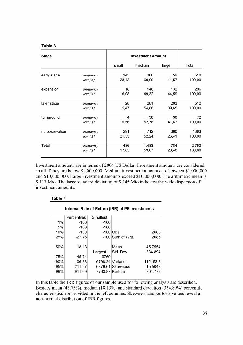
38
Table 3
Stage Investment Amount
small medium large Total
early stage frequency 145 306 59 510row [%] 28,43 60,00 11,57 100,00
expansion frequency 18 146 132 296row [%] 6,08 49,32 44,59 100,00
later stage frequency 28 281 203 512row [%] 5,47 54,88 39,65 100,00
turnaround frequency 4 38 30 72row [%] 5,56 52,78 41,67 100,00
no observation frequency 291 712 360 1363row [%] 21,35 52,24 26,41 100,00
Total frequency 486 1.483 784 2.753row [%] 17,65 53,87 28,48 100,00
Investment amounts are in terms of 2004 US Dollar. Investment amounts are considered small if they are below $1,000,000. Medium investment amounts are between $1,000,000 and $10,000,000. Large investment amounts exceed $10,000,000. The arithmetic mean is $ 117 Mio. The large standard deviation of $ 245 Mio indicates the wide dispersion of investment amounts.
Table 4
Internal Rate of Return (IRR) of PE investments
Percentiles Smallest1% -100 -1005% -100 -100
10% -100 -100 Obs 268525% -27.76 -100 Sum of Wgt. 2685
50% 18.13 Mean 45.7554Largest Std. Dev. 334.894
75% 45.74 676990% 106.88 6798.24 Variance 112153.895% 211.97 6879.61 Skewness 15.504899% 911.69 7763.87 Kurtosis 304.772
In this table the IRR figures of our sample used for following analysis are described. Besides mean (45.75%), median (18.13%) and standard deviation (334.89%) percentile characteristics are provided in the left columns. Skewness and kurtosis values reveal a non-normal distribution of IRR figures.

39
Table 5
Excess Return Benchmark IndexIRR based
S&P 500 Nasdaq Composite Russel2000 Dow Jones Ind. Avg. MSCI Worldobs mean std dev median mean std dev median mean std dev median mean std dev median mean std dev median
[%] [%] [%] [%] [%] [%] [%] [%] [%] [%] [%] [%] [%] [%] [%]
All investments 2380 36.63 353.81 2.99 29.79 350.96 -3.41 39.74 353.60 6.09 36.73 354.34 3.32 41.63 353.43 8.00
IndustryIT 361 84.22 597.28 -6.54 77.21 591.26 -10.13 88.23 596.78 -2.03 84.64 598.10 -6.24 89.32 596.52 -1.05consumer discretionary 273 14.00 97.71 8.00 7.88 98.25 3.03 18.02 97.86 11.75 14.03 98.03 8.25 19.47 97.93 13.68industrial production 323 11.51 103.55 7.13 3.49 104.05 -0.39 15.37 104.06 9.19 11.71 103.45 7.52 16.72 103.19 13.56telecommunication 151 66.53 269.98 2.45 57.52 260.77 -2.84 69.01 270.43 11.35 66.53 271.72 3.95 71.06 269.26 6.68services 172 11.39 201.38 -0.20 4.75 204.78 -9.40 14.78 202.57 3.38 11.48 201.07 -0.94 16.81 202.34 2.23healthcare 288 38.76 453.87 -2.54 31.72 449.84 -10.00 41.76 452.02 0.77 38.64 454.58 -3.21 43.65 453.14 1.69internet & media 232 63.26 509.19 2.57 55.81 506.81 -3.06 66.06 510.46 6.44 63.45 509.50 2.77 68.16 508.79 7.23other industry 580 18.74 205.99 3.23 13.27 205.17 -3.38 20.73 205.22 4.98 18.70 206.39 2.51 23.43 205.69 7.83
Stageearly stage 426 4.10 215.75 -27.06 -1.28 214.69 -33.21 7.43 217.44 -23.45 3.68 216.63 -26.81 9.13 215.85 -21.12expansion 263 21.01 116.12 7.55 14.40 114.61 0.52 25.13 115.46 12.71 21.22 116.73 7.64 26.77 115.61 13.72later stage 448 74.88 424.69 14.05 66.15 420.94 7.05 78.62 423.99 17.92 75.39 425.37 14.13 79.89 424.22 18.59turnaround 68 67.11 437.34 14.83 60.79 437.88 8.72 70.93 437.88 14.45 67.01 437.16 12.83 71.50 438.05 18.94no observation 1175 35.57 391.38 3.07 28.83 388.08 -3.28 38.09 390.93 5.24 35.70 391.83 2.88 40.41 390.84 7.30
Investment Amountsmall 373 76.70 591.98 -8.71 71.17 588.63 -12.22 80.36 592.10 -4.64 72.85 592.50 -9.12 81.81 591.39 -3.49medium 1300 39.32 362.06 1.15 32.08 358.49 -5.31 42.07 361.72 4.47 39.17 362.74 0.64 44.07 361.66 5.84large 707 13.95 102.70 9.17 6.08 101.10 2.56 17.26 101.94 11.92 14.42 103.17 10.03 19.25 102.55 14.84
In this table we summarize the appraisal of PE investments relative to five different broad public equity benchmarks. Excess returns of PE investments over the benchmarks are based on IRR differences between the PE and simulated investments in the benchmark. We distinguish industries, stages and size to analyze structural differences. Market quotes are obtained from the records of Bloomberg and Datastream. Table 6
PME Benchmark Index
S&P 500 Nasdaq Composite Russel2000 Dow Jones Ind. Avg. MSCI Worldobs mean std dev median mean std dev median mean std dev median mean std dev median mean std dev median
All investments 2470 3.01 22.29 1.05 2.75 22.44 0.93 3.40 25.85 1.13 3.05 22.66 1.05 3.35 24.63 1.17
IndustryIT 382 2.96 8.18 0.78 2.58 7.50 0.66 3.32 9.49 0.85 3.05 8.63 0.76 3.33 9.25 0.94consumer discretionary 290 1.98 7.48 1.17 1.82 6.71 1.06 2.15 7.51 1.29 1.96 7.34 1.17 2.21 7.61 1.31industrial production 333 2.03 7.74 1.13 1.75 6.84 0.99 2.20 7.74 1.22 2.00 7.17 1.14 2.25 7.25 1.29telecommunication 163 3.19 10.10 1.00 2.58 8.22 0.87 3.82 13.67 1.04 3.31 10.68 0.97 3.48 10.78 1.05services 180 1.28 1.37 0.99 1.24 1.57 0.84 1.40 1.47 1.06 1.26 1.32 0.98 1.45 1.56 1.04healthcare 293 7.00 46.05 0.88 7.00 48.43 0.73 8.02 54.32 1.05 7.18 48.28 0.86 7.48 47.90 1.10internet & media 239 2.82 10.75 1.07 2.19 7.37 0.94 3.34 14.17 1.12 2.90 11.48 1.08 3.15 12.44 1.19other industry 590 2.68 28.85 1.06 2.49 28.34 0.95 2.94 32.57 1.11 2.65 28.10 1.05 3.10 34.28 1.16
Stageearly stage 442 2.52 9.87 0.40 2.08 7.69 0.35 3.11 13.51 0.45 2.63 10.64 0.40 2.90 11.43 0.45expansion 276 1.87 3.75 1.11 1.63 2.78 0.99 2.12 4.75 1.26 1.87 3.92 1.13 2.15 4.08 1.29later stage 469 2.42 7.00 1.32 2.16 6.05 1.14 2.61 7.18 1.46 2.42 6.92 1.32 2.64 7.10 1.49turnaround 71 11.31 83.34 1.31 11.02 81.93 1.13 12.68 94.09 1.32 11.03 81.16 1.28 13.31 99.05 1.39no observation 1212 3.20 23.43 1.04 2.99 24.43 0.93 3.55 27.45 1.12 3.25 24.47 1.04 3.47 24.35 1.17
Investment Amountsmall 385 8.95 55.89 0.85 8.70 56.70 0.74 10.28 64.73 0.91 9.10 56.77 0.83 9.79 61.83 0.97medium 1343 2.24 6.40 1.00 1.90 5.32 0.84 2.50 7.67 1.07 2.27 6.66 0.98 2.50 6.94 1.12large 742 1.56 1.67 1.20 1.42 1.63 1.05 1.71 1.85 1.28 1.55 1.63 1.20 1.79 1.91 1.34
Here we appraise PE investments relative to five different broad public equity benchmarks based on the Public Market Equivalent (PME) concept. In contrast to IRR, the PME assumes a reinvestment of intermediate cash flows in the public benchmark. PMEs exceeding (below) one indicate a relative outperformance (underperformance) of PE.

40
Table 7
Benchmark Index
S&P 500 Nasdaq Composite Russel2000 Dow Jones Ind. Avg. MSCI World
observations 2,380 2,380 2,380 2,380 2,380different outperformance conclusion [%] 0.42 1.18 0.21 0.42 0.21excess return > 0 & PME < 1 3 2 2 3 1excess return < 0 & PME > 1 7 26 3 7 4
In this table we investigate the impact of the reinvestment hypothesis on the conclusion whether PE outperforms the public benchmark or not. Excess return and PME are used as performance measures respectively. If excess returns are positive (negative) and PMEs is below (exceeds) one, a different outperformance conclusion is noted. The table solely tackles the direction of outperformance, not the degree. It can be observed that the reinvestment assumption rarely (in less than 1.1% of all cases) alters the conclusion about the direction of outperformance. Table 8
Deviation of excess return Benchmark Index
S&P 500 Nasdaq Composite Russel2000 Dow Jones Ind. Avg. MSCI Worldobs dev share IRR > dev share IRR > dev share IRR > dev share IRR > dev share IRR >
[%] PME [%] PME [%] PME [%] PME [%] PME
All investments10% 2380 665 28 428 632 27 371 694 29 463 668 28 431 688 29 47425% 2380 320 13 246 306 13 219 318 13 254 319 13 249 323 14 25950% 2380 175 7 157 171 7 149 181 8 163 177 7 159 183 8 165
Absolute differences in percentage points between excess return based on IRR and excess return based on PME are in the scope of this table. For five broad benchmarks a deviation (dev) is noted if the return difference exceeds the significance level (10%, 25%, 50%). Our results reveal substantial impact of the reinvestment hypothesis for the appraisal of PE investments. For more than 27% of the PE investments excess returns deviate by more than 10% depending on the reinvestment hypothesis. If the significance level is raised to 50% still more than 7% of the investments exceed this level. IRR based excess returns substantially overstate the performance of PE investments. In more than 64% of all deviations (for the 10% significance level relative to S&P 500) the assumed reinvestment in equivalent PE ventures of the IRR concept significantly increases excess returns in comparison to a reinvestment in the public index (PME). This share increases with the significance level and reaches 90% for deviations exceeding 50% (again relative to S&P 500).

41
Table 9
Excess Return Benchmark IndexPME based
S&P 500 Nasdaq Composite Russel2000 Dow Jones Ind. Avg. MSCI Worldobs mean std dev median mean std dev median mean std dev median mean std dev median mean std dev median
[%] [%] [%] [%] [%] [%] [%] [%] [%] [%] [%] [%] [%] [%] [%]
All investments 2380 10.14 166.47 2.00 5.71 167.54 -1.83 12.40 166.35 4.05 10.06 166.51 2.31 13.88 165.83 5.56
IndustryIT 361 7.59 145.91 -4.41 3.75 148.71 -8.33 10.27 145.84 -1.44 7.58 146.04 -4.77 11.56 145.24 -0.65consumer discretionary 273 10.02 88.38 5.83 5.74 89.07 2.35 13.08 88.42 7.71 9.94 88.47 5.35 14.02 88.46 8.91industrial production 323 4.22 77.88 4.42 -1.43 79.44 0.29 6.84 77.12 6.76 4.38 78.08 5.82 8.07 77.29 8.20telecommunication 151 23.51 151.82 1.68 19.21 152.33 -2.35 25.47 151.98 8.08 23.00 152.73 3.07 27.07 151.34 4.15services 172 -9.62 57.47 -0.14 -15.20 60.37 -6.40 -7.39 57.56 2.23 -9.57 57.94 -0.45 -5.96 56.50 1.62healthcare 288 19.73 334.99 -2.24 14.79 336.50 -7.36 22.59 335.60 0.69 19.47 334.20 -2.48 23.73 334.21 1.39internet & media 232 19.60 157.25 1.66 15.49 158.00 -1.93 21.58 157.28 5.49 19.63 157.75 1.87 23.54 156.73 5.40other industry 580 8.23 143.90 2.24 4.25 143.51 -1.43 9.59 142.79 2.88 8.07 144.34 2.13 11.55 142.82 5.24
Stageearly stage 426 -19.53 96.69 -21.66 -23.01 98.55 -25.92 -17.26 97.14 -17.51 -20.18 96.39 -21.19 -15.50 95.93 -16.40expansion 263 11.74 94.36 4.77 7.09 93.22 0.26 14.68 93.90 8.22 11.89 94.90 5.67 15.88 93.71 9.12later stage 448 40.91 290.90 9.57 36.14 295.11 4.64 43.52 291.53 12.28 41.10 290.43 9.65 44.48 290.54 13.28turnaround 68 34.51 238.28 7.46 30.67 238.85 4.86 36.41 236.48 10.14 34.06 238.73 8.11 36.70 235.64 11.19no observation 1175 7.41 120.83 1.89 2.87 120.50 -1.67 9.38 120.02 3.72 7.39 121.09 2.17 11.10 120.07 5.08
Investment Amountsmall 373 21.58 211.25 -6.21 17.90 210.32 9.95 24.46 209.94 -4.27 21.53 211.69 -7.15 25.80 209.73 -2.45medium 1300 9.00 189.75 0.88 4.92 192.24 -3.42 10.98 190.17 3.19 8.68 189.59 0.54 12.65 189.30 4.25large 707 6.55 83.77 5.50 1.11 81.99 1.85 8.88 82.85 7.89 6.82 84.15 5.96 10.20 83.22 9.12
In this table we summarize the appraisal of PE investments relative to five different broad public equity benchmarks. Excess returns of PE investments over the benchmarks are derived from PME figures according to the model illustrated in appendix B. We distinguish industries, stages and size to analyze structural differences. Table 10
Excess return distribution realtive to Nasday Composite Index
IRR based computation PME based computation
Percentiles Smallest Percentiles Smallest 1% -152.5541 -270.8378 1% -143.9208 -265.9287 5% -126.9742 -230.7748 5% -117.8298 -221.966610% -108.7087 -225.1567 Obs 2380 10% -92.04899 -205.9667 Obs 238025% -44.79809 -209.3528 Sum of Wgt. 2380 25% -28.53416 -184.4794 Sum of Wgt. 2380
50% -3.412843 Mean 29.7933 50% -1.82974 Mean 5.71054 Largest Std. Dev. 350.9595 Largest Std. Dev. 167.54275% 26.41874 6699.065 75% 18.97827 1369.32790% 88.71028 6742.072 Variance 123172.6 90% 61.99697 1953.427 Variance 28070.3495% 204.4509 6833.965 Skewness 14.82416 95% 110.565 2119.202 Skewness 17.1215999% 962.2832 7658.873 Kurtosis 276.0529 99% 535.6398 5398.333 Kurtosis 480.2083

42
Table 11
Excess Returns Specific Benchmarks Nasdaq Compositespecific benchmarksPME based Specific benchmark PME based excess return PME based excess return
obs mean std dev median mean std dev median[%] [%] [%] [%] [%] [%]
IndustryIT S&P IT 228 10.64 180.51 -14.59 15.6 180.2 -8.3consumer discretionary S&P Consumers 116 6.88 58.71 6.53 2.4 60.2 2.3industrial production S&P Industrials 322 2.69 74.75 3.68 -2.8 75.9 0.2telecommunication Nasdaq Teleco. 150 21.39 152.79 -1.22 19.4 152.8 -1.7healthcare S&P Healthcare 129 57.01 498.25 -3.70 52.2 498.5 -9.8
GeographyGermany DAX 104 10.57 117.57 2.44 10.16 120.34 1.15UK FTSE UK 100 342 9.10 122.58 7.65 1.01 125.35 1.53
Here we compare excess returns of PE investments relative to specific (industry and local) and broad (Nasdaq Composite) indices. As we reduce our sample to ensure comparability, the second column contains comparable excess returns of the PE investments over the Nasdaq Composite Index. Excess returns are derived from PME figures according to the model illustrated in appendix B. The choice of benchmark rarely impacts direction but substantially the degree of relative performance.
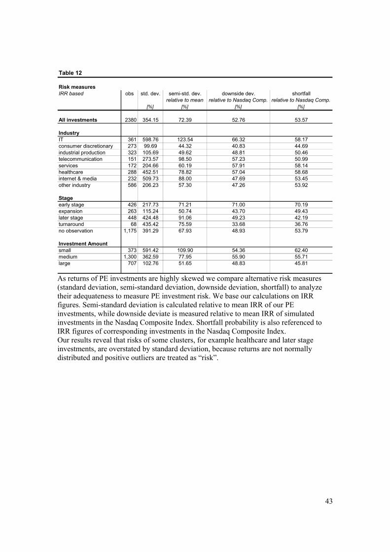
43
Table 12
Risk measuresIRR based obs std. dev. semi-std. dev. downside dev. shortfall
relative to mean relative to Nasdaq Comp. relative to Nasdaq Comp.[%] [%] [%] [%]
All investments 2380 354.15 72.39 52.76 53.57
IndustryIT 361 598.76 123.54 66.32 58.17consumer discretionary 273 99.69 44.32 40.83 44.69industrial production 323 105.69 49.62 48.81 50.46telecommunication 151 273.57 98.50 57.23 50.99services 172 204.66 60.19 57.91 58.14healthcare 288 452.51 78.82 57.04 58.68internet & media 232 509.73 88.00 47.69 53.45other industry 586 206.23 57.30 47.26 53.92
Stageearly stage 426 217.73 71.21 71.00 70.19expansion 263 115.24 50.74 43.70 49.43later stage 448 424.48 91.06 49.23 42.19turnaround 68 435.42 75.59 33.68 36.76no observation 1,175 391.29 67.93 48.93 53.79
Investment Amountsmall 373 591.42 109.90 54.36 62.40medium 1,300 362.59 77.95 55.90 55.71large 707 102.76 51.65 48.83 45.81
As returns of PE investments are highly skewed we compare alternative risk measures (standard deviation, semi-standard deviation, downside deviation, shortfall) to analyze their adequateness to measure PE investment risk. We base our calculations on IRR figures. Semi-standard deviation is calculated relative to mean IRR of our PE investments, while downside deviate is measured relative to mean IRR of simulated investments in the Nasdaq Composite Index. Shortfall probability is also referenced to IRR figures of corresponding investments in the Nasdaq Composite Index. Our results reveal that risks of some clusters, for example healthcare and later stage investments, are overstated by standard deviation, because returns are not normally distributed and positive outliers are treated as “risk”.

44
Table 13
Sharpe RatiosIRR based PE investments PM investments Differences (mean)
obs std. dev. Sharpe Ratio std. dev. Sharpe Ratio absolute difference Outperformermean median max mean median max PE- PM
All investments 2380 354.15 0.13 0.04 21.90 21.53 0.70 0.69 7.65 -0.58 PM
IndustryIT 361 598.76 0.15 0.00 12.98 24.22 0.61 0.63 6.15 -0.46 PMconsumer discretionary 273 99.69 0.24 0.18 11.24 17.99 0.86 0.85 7.08 -0.62 PMindustrial production 323 105.69 0.20 0.16 9.29 17.74 0.98 0.88 6.13 -0.79 PMtelecommunication 151 273.57 0.27 0.05 7.46 31.15 0.51 0.64 5.28 -0.24 PMservices 172 204.66 0.10 0.05 11.55 23.21 0.68 0.68 5.24 -0.58 PMhealthcare 288 452.51 0.10 0.01 14.98 19.32 0.78 0.76 6.11 -0.68 PMinternet & media 232 509.73 0.14 0.02 13.47 27.55 0.56 0.57 5.75 -0.42 PMother industry 580 206.23 0.13 0.06 17.26 17.31 0.79 0.80 4.29 -0.66 PM
Stageearly stage 426 217.73 0.05 -0.08 13.56 27.93 0.43 0.57 5.89 -0.38 PMexpansion 263 115.24 0.26 0.14 7.82 20.54 0.77 0.84 4.98 -0.51 PMlater stage 448 424.48 0.20 0.06 15.98 22.60 0.80 0.81 7.00 -0.60 PMturnaround 68 435.42 0.17 0.05 8.13 16.89 0.80 0.81 3.41 -0.64 PMno observation 1175 391.29 0.11 0.03 19.82 18.58 0.81 0.74 8.52 -0.70 PM
Investment Amountsmall 373 591.42 0.14 0.00 11.61 19.81 0.69 0.68 7.58 -0.55 PMmedium 1300 362.59 0.13 0.03 21.38 22.78 0.63 0.65 7.23 -0.50 PMlarge 707 102.76 0.23 0.19 10.39 20.75 0.83 0.76 7.63 -0.60 PM
GeogrpahyGermany 104 782.68 0.15 0.02 9.91 18.98 0.88 0.99 5.22 -0.73 PMUK 342 207.69 0.12 0.08 17.16 20.56 0.79 0.75 7.68 -0.67 PM
To appraise PE investments relative PM on a risk adjusted basis we calculate the Sharpe Ratio for our entire sample and all clusters. As standard deviation overstates investment risks of PE, we are not surprised to observe substantially higher Sharpe Ratios for PM investments. Based on these results, PM outperform PE investment by a considerable margin.

45
Table 14
Modified Sharpe RatiosIRR based PE investments PM investments (Nasdaq Comp.)Differences (mean)downside deviation (dwn.dev.) obs dwn. dev. mod. Sharpe Ratio dwn. dev. mod. Sharpe Ratio absolute difference Outperformerrelative to 2 yrs US Gov [%] mean median max [%] mean median max PE- PM
All investments 2380 45.74 0.98 0.29 169.61 9.77 1.54 1.52 16.85 -0.56 PM
IndustryIT 361 57.98 1.59 0.05 133.88 11.75 1.26 1.33 12.79 0.33 PEconsumer discretionary 273 33.87 0.69 0.51 32.36 6.99 2.21 2.18 18.22 -1.52 PMindustrial production 323 39.67 0.51 0.41 24.12 6.73 2.47 2.31 16.15 -1.97 PMtelecommunication 151 51.03 1.44 0.27 39.93 14.03 1.14 1.42 11.74 0.30 PEservices 172 48.25 0.42 0.20 48.80 9.03 1.74 1.74 13.47 -1.31 PMhealthcare 288 49.10 0.95 0.11 138.32 7.79 1.93 1.88 15.16 -0.98 PMinternet & media 232 42.10 1.69 0.27 163.29 12.99 1.18 1.21 12.20 0.51 PEother industry 580 42.98 0.63 0.31 82.94 9.09 1.51 1.52 8.17 -0.88 PM
Stageearly stage 426 63.67 0.17 -0.28 46.63 15.00 0.81 1.05 10.98 -0.64 PMexpansion 263 35.38 0.85 0.47 25.52 9.91 1.60 1.75 10.32 -0.74 PMlater stage 448 40.29 2.08 0.59 168.57 8.52 2.11 2.14 18.56 -0.03 PMturnaround 68 30.04 2.47 0.72 118.66 8.17 1.66 1.67 7.06 0.81 PEno observation 1175 42.63 1.03 0.28 181.93 7.63 1.97 1.81 20.76 -0.94 PM
Investment Amountsmall 373 49.00 1.73 0.02 140.29 8.78 1.57 1.54 17.12 0.17 PEmedium 1300 48.94 0.96 0.23 158.52 11.19 1.28 1.33 14.71 -0.32 PMlarge 707 40.32 0.58 0.49 26.50 7.78 2.21 2.02 20.36 -1.63 PM
GeogrpahyGermany 104 52.27 2.25 0.33 148.42 9.30 1.80 2.03 10.65 0.44 PEUK 342 43.34 0.58 0.39 82.25 7.06 2.30 2.17 22.40 -1.72 PM
To better suit the characteristics of PE returns, we modify the Sharpe Ratio and measure risk in terms of downside deviation rather than standard deviation. The modified Sharpe Ratio accounts for both, probability and magnitude of the shortfall relative to the return of the 2 year US Government bonds. As we are interested in cross sectional differences we assign the cluster’s downside deviation of returns to all investments belonging to the cluster. For the PM returns we use the IRRs of the simulated investments in the Nasdaq Composite Index and corresponding excess returns over the Government bonds. Our adjustment of the Sharpe Ratio triggered a substantial increase of mean values, 680% and 119% for PE and PM investments respectively. The substantially larger increase for PE supports our hypothesis that standard deviation overstates PE’s investment risk in our relative analysis. Mean and median ratios indicate underformance of PE as an asset class relative to investments in the Nasdaq Composite for the overall sample and the average investment. The ratios of the PE clusters reveal very heterogeneous risk adjusted performance. While turnaround and later stage investment outperform or match the performance of the Nasdaq Composite Index, early stage and expansion investments substantially underperform.

46
Table 15
Modified Sharpe RatiosIRR based PE investments PM investments Differences (mean)Shortfall obs shortfall mod. Sharpe Ratio shortfall mod. Sharpe Ratio absolute difference Outperformerrelative to 2 yrs US Gov [%] mean median max [%] mean median max PE- PM
All investments 2380 35.97 1.25 0.37 215.68 13.66 1.11 1.09 12.05 0.14 PE
IndustryIT 361 46.81 1.97 0.06 165.73 17.73 0.84 0.88 8.47 1.13 PEconsumer discretionary 273 21.61 1.08 0.80 50.73 10.99 1.41 1.39 11.59 -0.33 PMindustrial production 323 32.82 0.61 0.50 29.14 9.29 1.79 1.68 11.70 -1.18 PMtelecommunication 151 35.76 2.05 0.38 56.98 21.85 0.73 0.91 7.54 1.33 PEservices 172 40.70 0.50 0.24 57.85 16.28 0.96 0.96 7.47 -0.46 PMhealthcare 288 44.10 1.06 0.12 154.01 15.28 0.98 0.96 7.72 0.08 PEinternet & media 232 38.79 1.83 0.29 177.22 15.95 0.96 0.99 9.93 0.87 PEother industry 580 32.25 0.84 0.41 110.53 10.07 1.36 1.38 7.38 -0.53 PM
Stageearly stage 426 59.39 0.18 -0.30 49.76 23.24 0.52 0.68 7.08 -0.34 PMexpansion 263 29.28 1.03 0.57 30.84 11.79 1.34 1.47 8.67 -0.31 PMlater stage 448 26.12 3.22 0.90 260.02 12.72 1.41 1.43 12.43 1.81 PEturnaround 68 22.06 3.37 0.99 161.59 13.24 1.03 1.03 4.36 2.35 PEno observation 1175 33.53 1.31 0.36 231.37 10.98 1.37 1.26 14.43 -0.06 PM
Investment Amountsmall 373 28.49 2.98 0.03 241.28 15.04 0.91 0.90 9.99 2.07 PEmedium 1300 38.63 1.22 0.29 200.83 15.16 0.94 0.98 10.86 0.27 PElarge 707 28.49 0.82 0.69 37.51 11.01 1.56 1.43 14.39 -0.74 PM
GeogrpahyGermany 104 32.69 3.59 0.52 237.31 8.65 1.94 2.18 11.46 1.65 PEUK 342 28.65 0.88 0.59 124.42 11.99 1.35 1.28 13.46 -0.48 PM
To test the impact of the magnitude of shortfall, we substitute downside deviation by shortfall probability and re-run our modified Sharpe Ratio analysis. The modified Sharpe Ratio now accounts for shortfall probability relative to the return of the 2 year US Government bonds only. As we are interested in cross sectional differences we assign the cluster’s shortfall probability to all investments belonging to the cluster. For the PM returns we use the IRRs of the simulated investments in the Nasdaq Composite Index and corresponding excess returns over the Government bonds. Mean ratios now indicate an overall outperformance of PE as an asset class, while median ratios are lower compared to their PM counterparts revealing underperformance of the average investment. The ratios of the PE clusters reveal very heterogeneous risk adjusted performance. While turnaround and later stage investment substantially outperform the Nasdaq Composite Index, early stage and expansion investments still underperform.

47
Table 16
OmegaPME based Nasdaq Composite Index Difference to PM S&P 500 Difference to PMRT > Benchmark obs G L Omega (Omega = 1) G L Omega (Omega = 1)
[mio US$] [mio US$] Outperformer [mio US$] [mio US$] Outperformer
All Investments 2,380 5,630 -5,670 0.99 -0.01 PM 6,310 -4,970 1.27 0.27 PE
IndustryIT 361 831 -1,070 0.78 -0.22 PM 859 -1,010 0.85 -0.15 PMconsumer discretionary 273 664 -735 0.90 -0.10 PM 734 -604 1.22 0.22 PEindustrial production 323 681 -758 0.90 -0.10 PM 769 -606 1.27 0.27 PEtelecommunication 151 392 -315 1.24 0.24 PE 425 -308 1.38 0.38 PEservices 172 222 -435 0.51 -0.49 PM 253 -363 0.70 -0.30 PMhealthcare 288 609 -759 0.80 -0.20 PM 658 -661 1.00 0.00 PMinternet & media 232 1,040 -550 1.89 0.89 PE 1,290 -492 2.62 1.62 PEother industry 580 1,100 -1,070 1.03 0.03 PE 1,250 -957 1.31 0.31 PE
Stageearly stage 426 323 -1,180 0.27 -0.73 PM 358 -1,110 0.32 -0.68 PMexpansion 263 758 -598 1.27 0.27 PE 898 -540 1.66 0.66 PElater stage 448 2,090 -1,490 1.40 0.40 PE 2,280 -1,340 1.70 0.70 PEturnaround 68 61 -119 0.51 -0.49 PM 76 -112 0.68 -0.32 PMno observation 1,175 2,400 -2,280 1.05 0.05 PE 2,700 -1,870 1.44 0.44 PE
Investment Amountsmall 373 74 -62 1.20 0.20 PE 78 -59 1.32 0.32 PEmedium 1,300 1,430 -1,380 1.04 0.04 PE 1,520 -1,240 1.23 0.23 PElarge 707 4,130 -4,230 0.98 -0.02 PM 4,720 -3,680 1.28 0.28 PE
GeogrpahyGermany 104 268 -166 1.61 0.61 PE 270 -149 1.81 0.81 PEUK 342 856 -1,080 0.79 -0.21 PM 985 -882 1.12 0.12 PE
Omega relates total excess chance to total shortfall risk. It is flexible regarding the reference point. We choose returns of investments in the Nasdaq Composite Index (left columns) and S&P 500 (right columns) as reference points, and consider all investments with a PME > 1 (PME < 1) as excess chance (shortfall risk). We calculate total annualized return of investment i as PME based annual excess return multiplied with the real investment amount (in terms of 2004 U.S. Dollars). Omega value weights all investments. Our results show a balanced shortfall risk and excess chance for PE investors relative to the Nasdaq Composite Index. As the outperformance of PM relative to PE is only minimal we are not surprised to see mixed results for out clusters. While later stage investments exhibit Omegas considerably exceeding one, early stage investments are the overall worst performing cluster. Switching to S&P 500 we observe higher Omegas indicating risk-adjusted outperformance of PE over public index. We conclude that PE investments generate an adequate return premium over PM investments gross of fess, as Omegas match one relative to the Nasdaq Composite Index and exceed one for all other benchmarks.
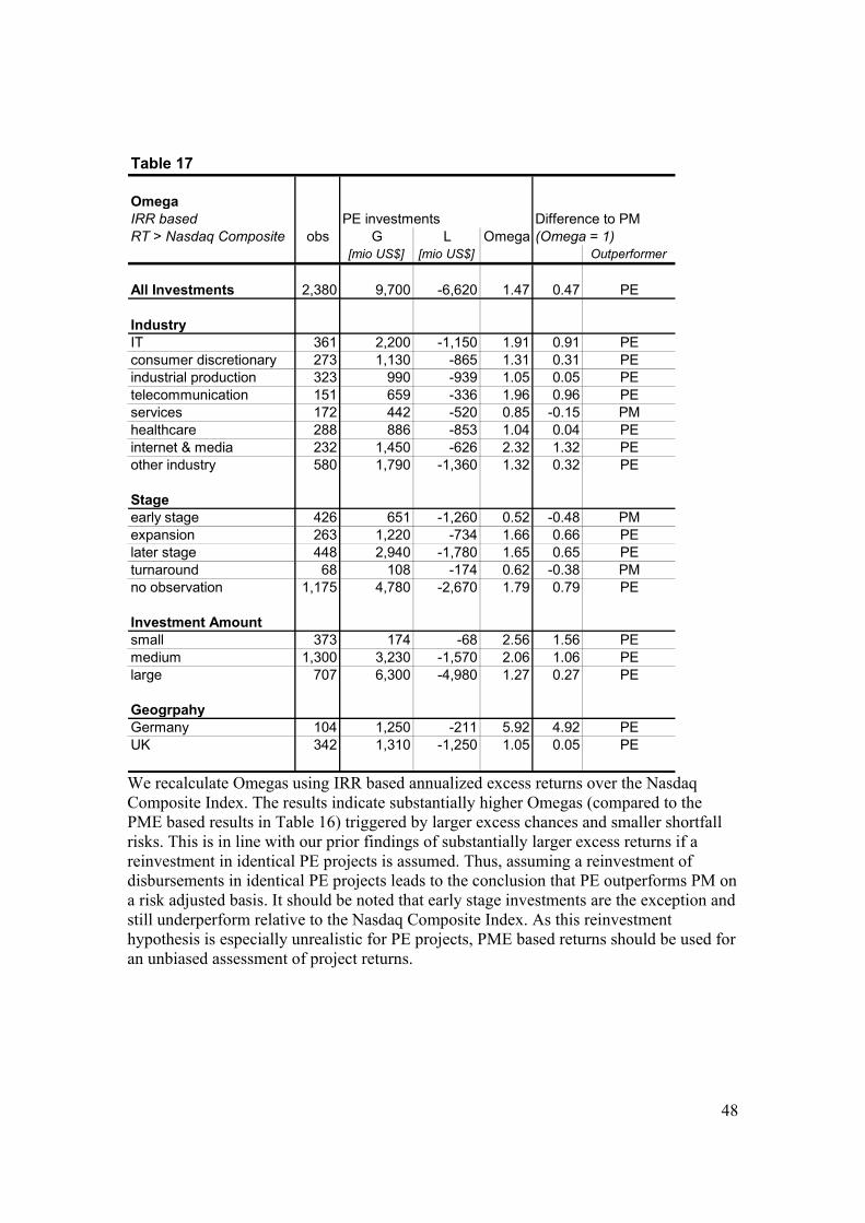
48
Table 17
OmegaIRR based PE investments Difference to PMRT > Nasdaq Composite obs G L Omega (Omega = 1)
[mio US$] [mio US$] Outperformer
All Investments 2,380 9,700 -6,620 1.47 0.47 PE
IndustryIT 361 2,200 -1,150 1.91 0.91 PEconsumer discretionary 273 1,130 -865 1.31 0.31 PEindustrial production 323 990 -939 1.05 0.05 PEtelecommunication 151 659 -336 1.96 0.96 PEservices 172 442 -520 0.85 -0.15 PMhealthcare 288 886 -853 1.04 0.04 PEinternet & media 232 1,450 -626 2.32 1.32 PEother industry 580 1,790 -1,360 1.32 0.32 PE
Stageearly stage 426 651 -1,260 0.52 -0.48 PMexpansion 263 1,220 -734 1.66 0.66 PElater stage 448 2,940 -1,780 1.65 0.65 PEturnaround 68 108 -174 0.62 -0.38 PMno observation 1,175 4,780 -2,670 1.79 0.79 PE
Investment Amountsmall 373 174 -68 2.56 1.56 PEmedium 1,300 3,230 -1,570 2.06 1.06 PElarge 707 6,300 -4,980 1.27 0.27 PE
GeogrpahyGermany 104 1,250 -211 5.92 4.92 PEUK 342 1,310 -1,250 1.05 0.05 PE
We recalculate Omegas using IRR based annualized excess returns over the Nasdaq Composite Index. The results indicate substantially higher Omegas (compared to the PME based results in Table 16) triggered by larger excess chances and smaller shortfall risks. This is in line with our prior findings of substantially larger excess returns if a reinvestment in identical PE projects is assumed. Thus, assuming a reinvestment of disbursements in identical PE projects leads to the conclusion that PE outperforms PM on a risk adjusted basis. It should be noted that early stage investments are the exception and still underperform relative to the Nasdaq Composite Index. As this reinvestment hypothesis is especially unrealistic for PE projects, PME based returns should be used for an unbiased assessment of project returns.

49
Appendix A We strive to generate cash flow patterns for public market investments that mimic our
private equity investments. As we do have detailed cash flow information for the PE
investments, a purchase (sale) of shares in the benchmark is simulated when a negative
(positive) cash flow occurs for the underlying PE investment. Doing so we achieve pairs
of public and private equity returns that are matched and thus comparable. To illustrate
our approach we use sample investment i of a private equity fund.
The monthly cash flow information forms the starting point for our model. In a first step
we look at the shares we need to purchase in the public benchmark investment b in period
t. When cash flows into the private equity investment we simulate an investment in the
public benchmark by purchasing an equivalent number of shares:
tb
titb P
CFISP =
with: tbSP = shares purchased of public benchmark investment b in period t
tiCFI = cash inflow of investment i in period t
tbP = price per share of benchmark investment b in period t
The total number of shares bought bSP over the entire holding period T then is:
∑=
=T
ttbb SPSP
0
We now add the sale of shares to our simulation. A sale occurs with a cash outflow
(distribution) from the private equity investment. To determine the number of shares to
be sold in period t we use the ratio of cash outflows in period t and total cash outflows
over T.
bi
titb SP
CFOCFO
SS ⋅=
with:

50
tbSS = shares sold of public benchmark investment b in period t
tiCFO = cash outflow of investment i in period t
iCFO = total cash outflows of investment i over holding period T
bSP = total number of shares in b bought over holding period T
Extreme cash flow patterns can trigger a simulated sale of more shares than have been
purchased previously. If for example a substantial cash outflow is followed by cash
inflows and a write-off, all shares would be sold when the cash outflow occurs and latter
“re-purchased” with the cash inflow. To avoid these misleading short sales we introduce
the following boundaries for the number of shares sold in period t:
bi
titb SP
CFOCFO
SS ⋅= bi
tibt SP
CFOCFO
Stb ⋅≥∀ − ,1:
bttb SSS ,1−= bi
tibt SP
CFOCFO
Stb ⋅<∀ − ,1:
with: ptS ,1− = shares held in benchmark investment b at the end of period t-1
In addition, a sale needs to be simulated if the private equity investment is completely
written off. We are not interested in partial write-offs during the holding period, but
solely in final write-offs marking the termination of investment i. After this point in time
no further cash in- or outflows occur. To appropriately reflect this fact, we simulate a sale
of all remaining shares of b in the period after the write-off. :
bttb SSS ,1−= iti WOCFt =∀ :
with: iWO = final and complete write-off of investment i
We can now track the number of shares held at the end of each period t. As we analyze
net cash flows, timing of share purchases and sales within a period does not matter. The
number of shares held at the end of period t is:
tbtbbttb SSSPSS −+= − ,1

51
The last step is to transform the time series of shares held into a cash flow stream. To do
so we multiply the change of shares held with the share price for each period t:
( ) tbtbbttb PSSCF ⋅−= − ,1
with:
tbCF = simulated cash flow of mimicked investment in benchmark b for private
equity investment i in period t
We have now generated the cash flow of an investment in a public benchmark that
mimics the corresponding investment in a private equity project. These cash flow pairs
enable us to perform cross sectional analysis between public and private equity. The
model is flexible with regard to both key parameters, the public benchmark and the
source of the cash flow stream. Besides cash flows of private equity projects, other
alternative asset classes can be used to enable a cross sectional analysis.

52
Appendix B In order to transform the PME ratio into return figures we start from the benchmark
index’s (public market) return:
11
−=−t
tit IV
IVy
with: ity = return of benchmark index i in period t
tIV = Index value in period t
If we assume discrete compounding and an investment horizon of T years, the total public
benchmark return iY is:
( )∏ =−+=
T
t iti yY1
11
As we analyze realized investments all inputs are known and certain. In a next step we
annualize the benchmark return:
( )[ ] 111
1−+= ∏ =
TT
t iti yy
The total return of PE investments j is:
10
−=j
jTi V
VX
with:
0jV = value of private equity investment j in period 0
jTV = value of private equity investment j in period T
Based on our PME definition, the following relationship must hold:
( )∏ =+⋅=
T
t itjij
jT yPMEVV
10
1
with: jiPME = Public Market Equivalent ratio of investment j relative to benchmark i

53
The terminal value of 1 $ investment in PE project j is equal to the terminal value of
jiPME $ in public benchmark i. If we annualize the PE return we get:
( )( ) 1111
1
1
0
−+⋅=−
= ∏ =
TT
t itji
T
j
jTi yPME
VV
x
The final step is to deduct the benchmark return as we are interested in excess returns
over the chosen benchmark. For the PME based excess return PMEER we get:
( )( ) ( )( )
−+−
−+⋅=−= ∏∏ ==
11111
1
1
1TT
t itTT
t itjiiiPMEj yyPMEyxER
( ) ( )( )TT
t itTjiPMEj yPMEER1
1
111 ∏=+⋅
−=
All inputs are available, as we can calculate ity for all investments and all benchmarks based on observable market quotes. We have also calculated the jiPME figures (please refer to Table 6).