periodogram and correlogram methods - tuttabus/course/advsp/21006lectures10_12.pdf · correlogram...

Periodogram

and

Correlogram

Methods

Lecture 2

Lecture notes to accompany Introduction to Spectral Analysis Slide L2–1by P. Stoica and R. Moses, Prentice Hall, 1997

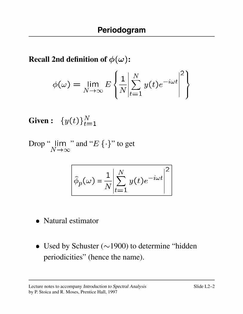
Periodogram

Recall 2nd definition of �(!):

�(!) = limN!1

E

8><>:1

N

��NXt=1

y(t)e�i!t

��29>=>;

Given : fy(t)gNt=1

Drop “ limN!1

” and “E f�g” to get

�p(!) =1

N

��NXt=1

y(t)e�i!t

��2

� Natural estimator

� Used by Schuster (�1900) to determine “hidden

periodicities” (hence the name).


Correlogram

Recall 1st definition of �(!):

�(!) =1X

k=�1

r(k)e�i!k

Truncate the “P

” and replace “r(k)” by “r(k)”:

�c(!) =N�1X

k=�(N�1)

r(k)e�i!k


Covariance Estimators(or Sample Covariances)

Standard unbiased estimate:

r(k) =1

N � k

NXt=k+1

y(t)y�(t� k); k � 0

Standard biased estimate:

r(k) =1

N

NXt=k+1

y(t)y�(t� k); k � 0

For both estimators:

r(k) = r�(�k); k < 0


Relationship Between �p(!) and �c(!)

If: the biased ACS estimator r(k) is used in �c(!),

Then:

�p(!) =1

N

��NXt=1

y(t)e�i!t

��2

=N�1X

k=�(N�1)

r(k)e�i!k

= �c(!)

�p(!) = �c(!)

Consequence:Both �p(!) and �c(!) can be analyzed simultaneously.


Statistical Performance of �p(!) and �c(!)

Summary:

� Both are asymptotically (for large N ) unbiased:

En�p(!)

o! �(!) as N !1

� Both have “large” variance, even for large N .

Thus, �p(!) and �c(!) have poor performance.

Intuitive explanation:

� r(k)� r(k) may be large for large jkj

� Even if the errors fr(k)� r(k)gN�1jkj=0

are small,

there are “so many” that when summed in

[�p(!)� �(!)], the PSD error is large.


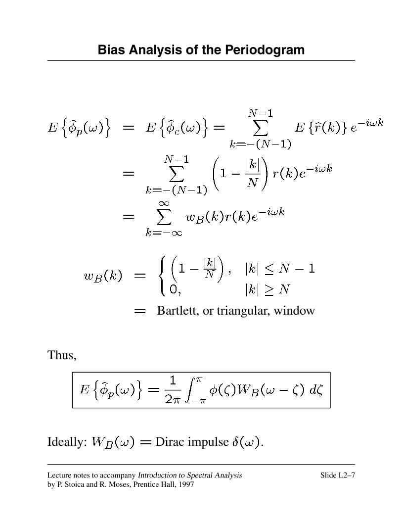
Bias Analysis of the Periodogram

En�p(!)

o= E

n�c(!)

o=

N�1Xk=�(N�1)

E fr(k)g e�i!k

=N�1X

k=�(N�1)

1�jkj

N

!r(k)e�i!k

=1X

k=�1

wB(k)r(k)e�i!k

wB(k) =

8<:�1�

jkjN

�; jkj � N � 1

0; jkj � N

= Bartlett, or triangular, window

Thus,

En�p(!)

o=

1

2�

Z ��

�(�)WB(! � �) d�

Ideally: WB(!) = Dirac impulse �(!).


Bartlett Window WB(!)

WB(!) =1

N

"sin(!N=2)

sin(!=2)

#2

WB(!)=WB(0), for N = 25

−3 −2 −1 0 1 2 3−60

−50

−40

−30

−20

−10

0

dB

ANGULAR FREQUENCY

Main lobe 3dB width� 1=N .

For “small” N , WB(!) may differ quite a bit from �(!).


Smearing and Leakage

Main Lobe Width: smearing or smoothing

Details in �(!) separated in f by less than 1=N are not

resolvable.φ(ω)

ω<1/Ν ω

φ(ω)^smearing

Thus: Periodogram resolution limit = 1=N .

Sidelobe Level: leakage

φ(ω)≅δ(ω)

ω ω

φ(ω)≅W (ω)^

leakage

B


Periodogram Bias Properties

Summary of Periodogram Bias Properties:

� For “small” N , severe bias

� As N !1, WB(!)! �(!),

so �(!) is asymptotically unbiased.


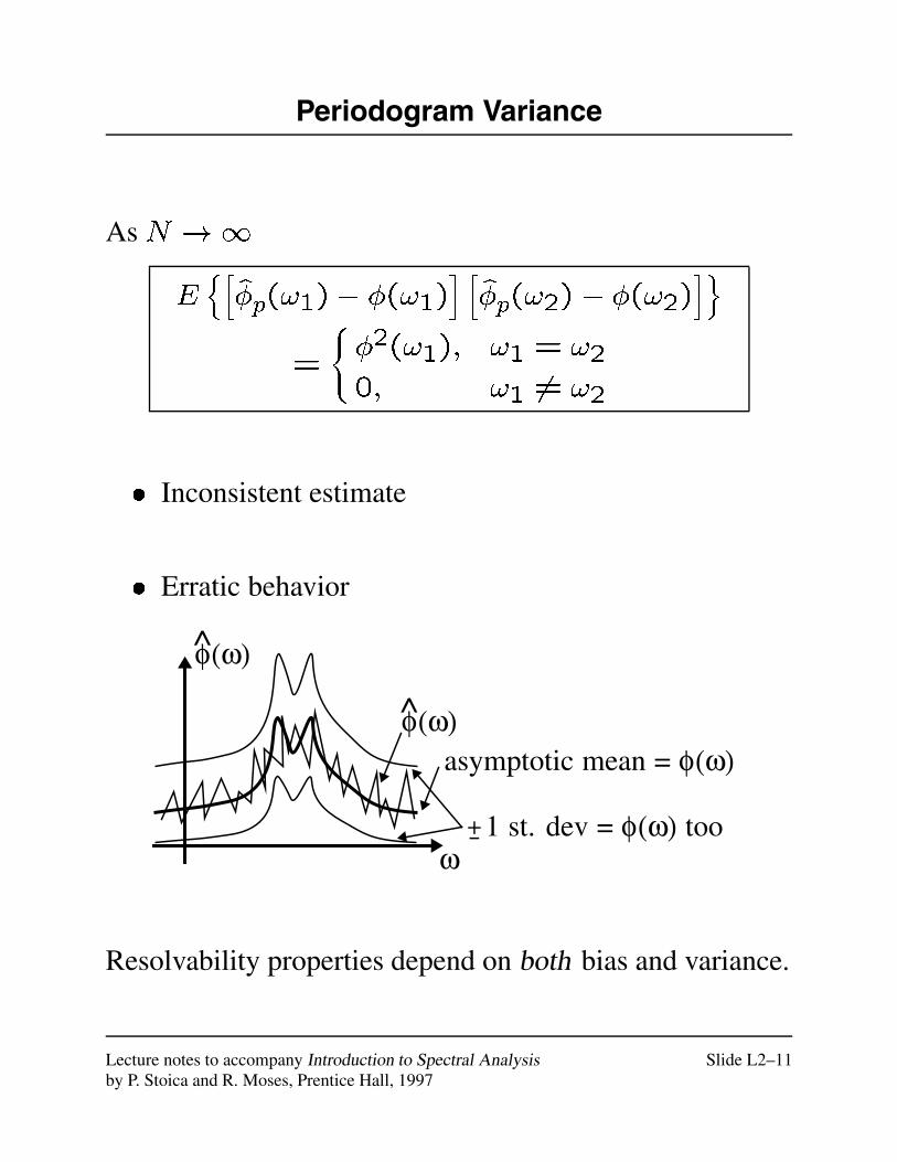
Periodogram Variance

As N !1

Enh�p(!1)� �(!1)

i h�p(!2)� �(!2)

io=

(�2(!1); !1 = !20; !1 6= !2

� Inconsistent estimate

� Erratic behavior

ω

φ(ω)^

1 st. dev = φ(ω) too +-

asymptotic mean = φ(ω)

φ(ω)^

Resolvability properties depend on both bias and variance.


Improved Periodogram-Based

Methods

Lecture 3


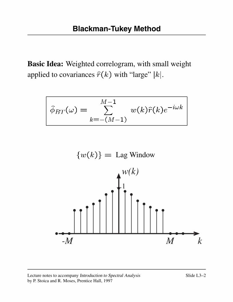
Blackman-Tukey Method

Basic Idea: Weighted correlogram, with small weight

applied to covariances r(k) with “large” jkj.

�BT (!) =M�1X

k=�(M�1)

w(k)r(k)e�i!k

fw(k)g = Lag Window

1

-M M

w(k)

k


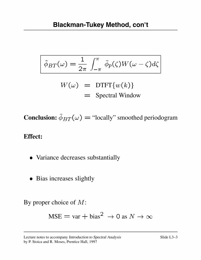
Blackman-Tukey Method, con't

�BT (!) =1

2�

Z ��

�p(�)W(! � �)d�

W(!) = DTFTfw(k)g

= Spectral Window

Conclusion: �BT (!) = “locally” smoothed periodogram

Effect:

� Variance decreases substantially

� Bias increases slightly

By proper choice of M :

MSE = var + bias2 ! 0 as N !1


Window Design Considerations

Nonnegativeness:

�BT (!) =1

2�

Z ��

�p(�)| {z }�0

W(! � �)d�

If W(!) � 0 (, w(k) is a psd sequence)

Then: �BT (!) � 0 (which is desirable)

Time-Bandwidth Product

Ne =

M�1Xk=�(M�1)

w(k)

w(0)= equiv time width

�e =

12�

Z ��

W(!)d!

W(0)= equiv bandwidth

Ne �e = 1


Window Design, con't

� �e = 1=Ne = 0(1=M)

is the BT resolution threshold.

� As M increases, bias decreases and variance

increases.

) Choose M as a tradeoff between variance and

bias.

� Once M is given, Ne (and hence �e) is essentially

fixed.

) Choose window shape to compromise between

smearing (main lobe width) and leakage (sidelobe

level).

The energy in the main lobe and in the sidelobes

cannot be reduced simultaneously, once M is given.


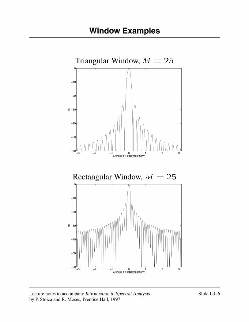
Window Examples

Triangular Window, M = 25

−3 −2 −1 0 1 2 3−60

−50

−40

−30

−20

−10

0dB

ANGULAR FREQUENCY

Rectangular Window, M = 25

−3 −2 −1 0 1 2 3−60

−50

−40

−30

−20

−10

0

dB

ANGULAR FREQUENCY


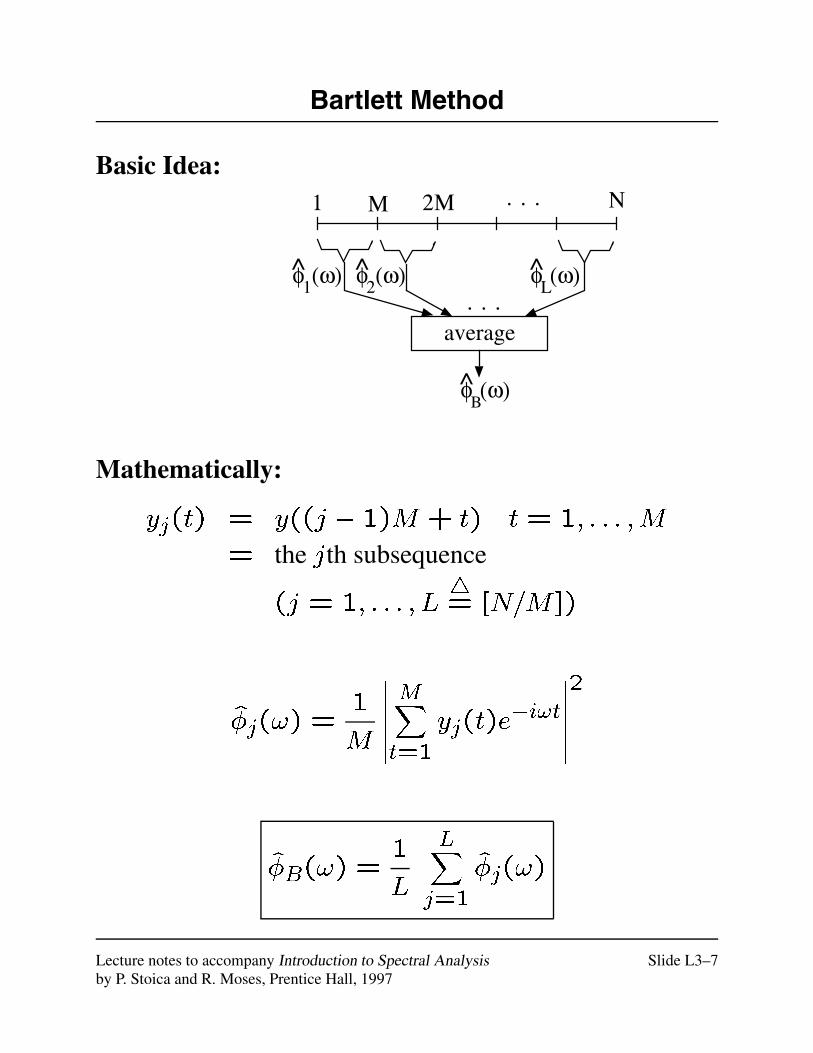
Bartlett Method

Basic Idea:1 Μ 2Μ Ν. . .

average. . .

φ (ω)1

φ (ω)2

φ (ω)L

φ (ω)B

Mathematically:

yj(t) = y((j � 1)M + t) t = 1; : : : ;M

= the jth subsequence

(j = 1; : : : ; L4= [N=M ])

�j(!) =1

M

��MXt=1

yj(t)e�i!t

��2

�B(!) =1

L

LXj=1

�j(!)


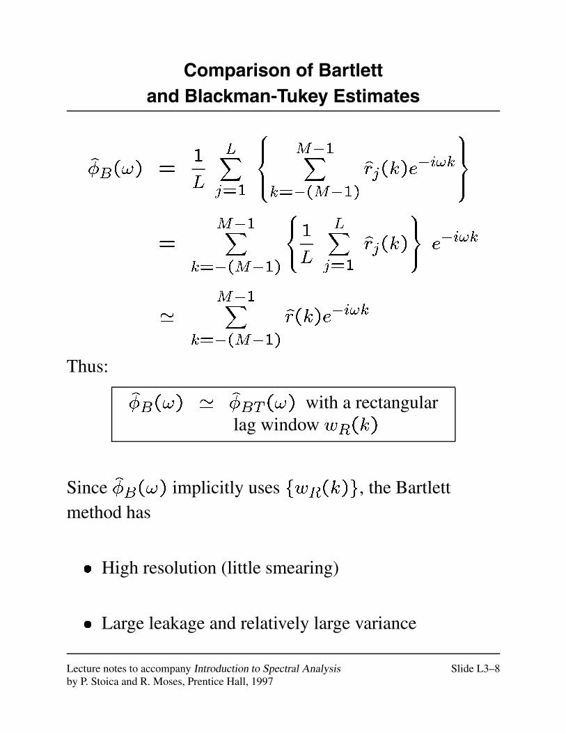
Comparison of Bartlettand Blackman-Tukey Estimates

�B(!) =1

L

LXj=1

8><>:

M�1Xk=�(M�1)

rj(k)e�i!k

9>=>;

=M�1X

k=�(M�1)

8<:1L

LXj=1

rj(k)

9=; e�i!k

'M�1X

k=�(M�1)

r(k)e�i!k

Thus:

�B(!) ' �BT (!) with a rectangularlag window wR(k)

Since �B(!) implicitly uses fwR(k)g, the Bartlettmethod has

� High resolution (little smearing)

� Large leakage and relatively large variance


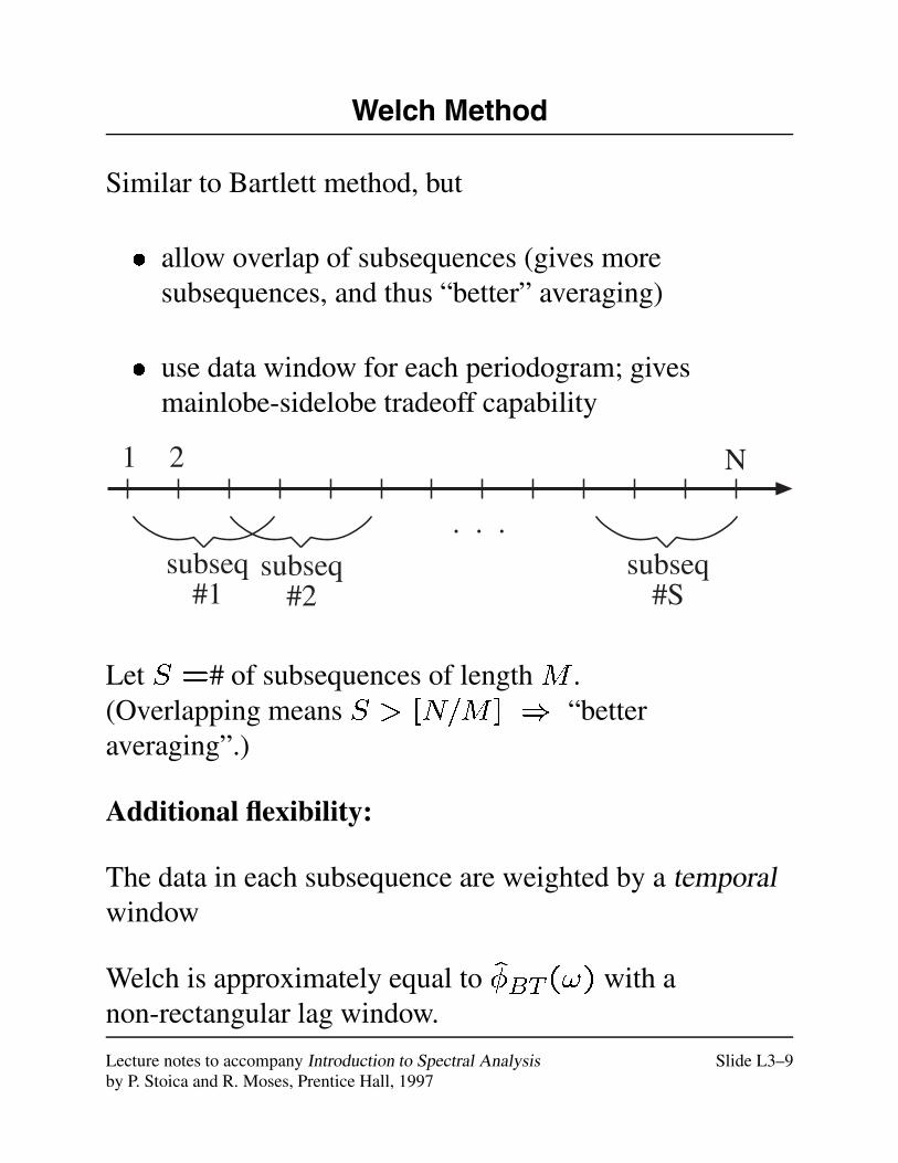
Welch Method

Similar to Bartlett method, but

� allow overlap of subsequences (gives moresubsequences, and thus “better” averaging)

� use data window for each periodogram; givesmainlobe-sidelobe tradeoff capability

1 2 N

subseq#1

. . .

subseq#2

subseq#S

Let S =# of subsequences of length M .(Overlapping means S > [N=M ] ) “betteraveraging”.)

Additional flexibility:

The data in each subsequence are weighted by a temporalwindow

Welch is approximately equal to �BT (!) with anon-rectangular lag window.


Daniell Method

By a previous result, for N � 1,

f�p(!j)g are (nearly) uncorrelated random variables for

�!j =

2�

Nj

�N�1j=0

Idea: “Local averaging” of (2J +1) samples in the

frequency domain should reduce the variance by about

(2J +1).

�D(!k) =1

2J +1

k+JXj=k�J

�p (!j)


Daniell Method, con't

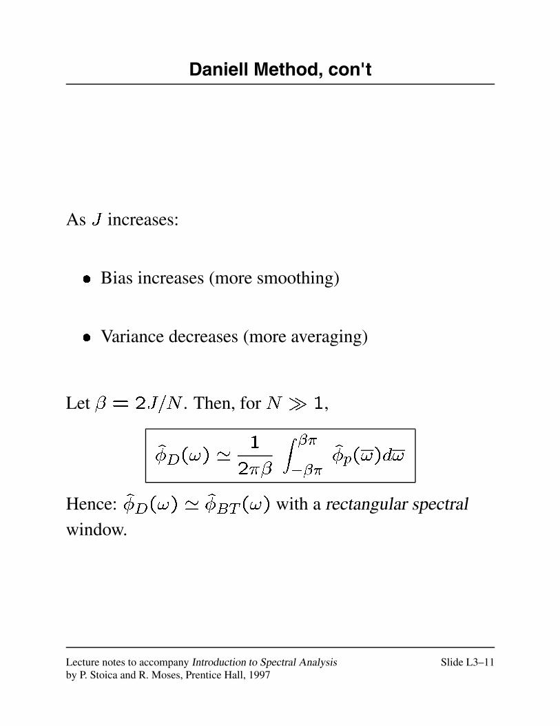
As J increases:

� Bias increases (more smoothing)

� Variance decreases (more averaging)

Let � = 2J=N . Then, for N � 1,

�D(!) '1

2��

Z ��

�p(!)d!

Hence: �D(!) ' �BT (!) with a rectangular spectralwindow.


Summary of Periodogram Methods

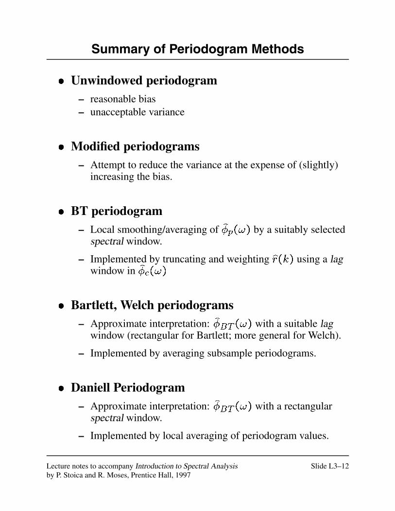
� Unwindowed periodogram– reasonable bias– unacceptable variance

� Modified periodograms– Attempt to reduce the variance at the expense of (slightly)

increasing the bias.

� BT periodogram– Local smoothing/averaging of �p(!) by a suitably selected

spectral window.

– Implemented by truncating and weighting r(k) using a lagwindow in �c(!)

� Bartlett, Welch periodograms– Approximate interpretation: �BT (!) with a suitable lag

window (rectangular for Bartlett; more general for Welch).

– Implemented by averaging subsample periodograms.

� Daniell Periodogram– Approximate interpretation: �BT (!) with a rectangular

spectral window.

– Implemented by local averaging of periodogram values.


Parametric Methods

for

Rational Spectra

Lecture 4


Basic Idea of Parametric Spectral Estimation

Observed Data

Assumed functional

form of φ(ω,θ)

Estimate parametersin φ(ω,θ)

Estimate PSD

φ(ω) =φ(ω,θ)^ ^θ

possibly revise assumption on φ(ω)

Rational Spectra

�(!) =

Pjkj�m ke

�i!kPjkj�n �ke

�i!k

�(!) is a rational function in e�i!.

By Weierstrass theorem, �(!) can approximate arbitrarilywell any continuous PSD, provided m and n are chosensufficiently large.

Note, however:

� choice of m and n is not simple

� some PSDs are not continuous


AR, MA, and ARMA Models

By Spectral Factorization theorem, a rational �(!) can be

factored as

�(!) =

��B(!)A(!)

��2

�2

A(z) = 1+ a1z�1+ � � �+ anz

�n

B(z) = 1+ b1z�1+ � � �+ bmz

�m

and, e.g., A(!) = A(z)jz=ei!

Signal Modeling Interpretation:e(t)

�e(!) = �2

white noise

y(t)

�y(!) =��

B(!)A(!)

��

2�2

B(q)

A(q)

�ltered white noise

--

ARMA: A(q)y(t) = B(q)e(t)

AR: A(q)y(t) = e(t)

MA: y(t) = B(q)e(t)


ARMA Covariance Structure

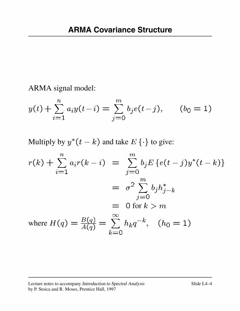
ARMA signal model:

y(t)+nXi=1

aiy(t� i) =mXj=0

bje(t�j); (b0 = 1)

Multiply by y�(t� k) and take E f�g to give:

r(k) +nXi=1

air(k � i) =mXj=0

bjE fe(t� j)y�(t� k)g

= �2mXj=0

bjh�j�k

= 0 for k > m

where H(q) = B(q)A(q)

=1Xk=0

hkq�k; (h0 = 1)


AR Signals: Yule-Walker Equations

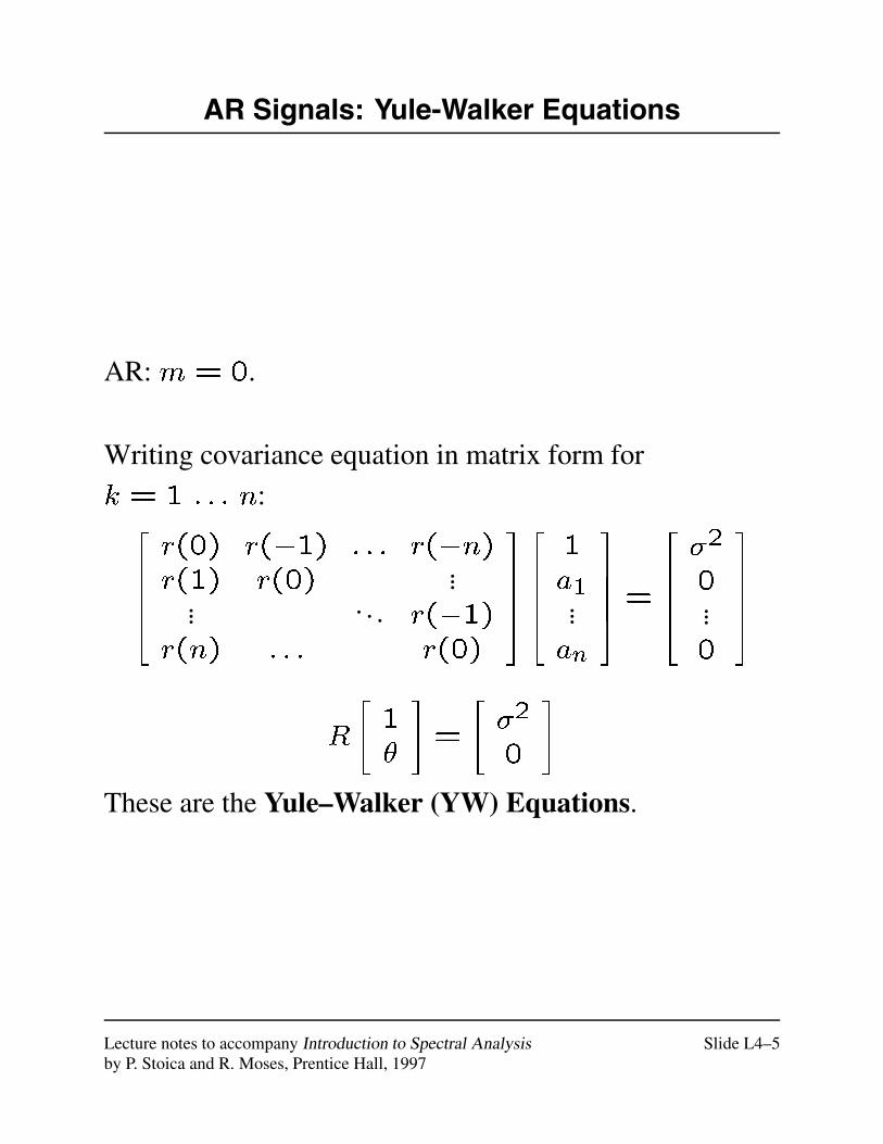
AR: m = 0.

Writing covariance equation in matrix form for

k = 1 : : : n:26664r(0) r(�1) : : : r(�n)r(1) r(0) ...

... . . . r(�1)r(n) : : : r(0)

3777526664

1a1...an

37775=

26664�2

0...0

37775

R

"1�

#=

"�2

0

#

These are the Yule–Walker (YW) Equations.


MA Signals

MA: n= 0

y(t) = B(q)e(t)

= e(t) + b1e(t� 1) + � � �+ bme(t�m)

Thus,

r(k) = 0 for jkj > m

and

�(!) = jB(!)j2�2 =mX

k=�m

r(k)e�i!k


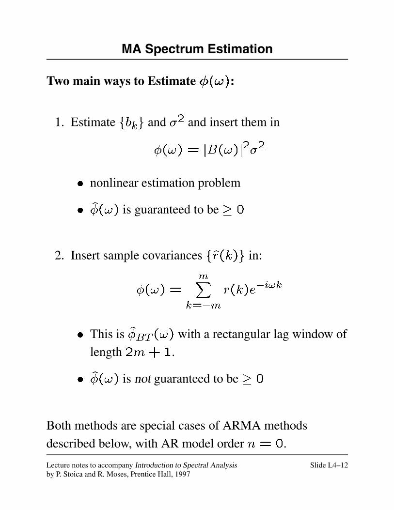
MA Spectrum Estimation

Two main ways to Estimate �(!):

1. Estimate fbkg and �2 and insert them in

�(!) = jB(!)j2�2

� nonlinear estimation problem

� �(!) is guaranteed to be� 0

2. Insert sample covariances fr(k)g in:

�(!) =mX

k=�m

r(k)e�i!k

� This is �BT (!) with a rectangular lag window of

length 2m+1.

� �(!) is not guaranteed to be� 0

Both methods are special cases of ARMA methods

described below, with AR model order n = 0.


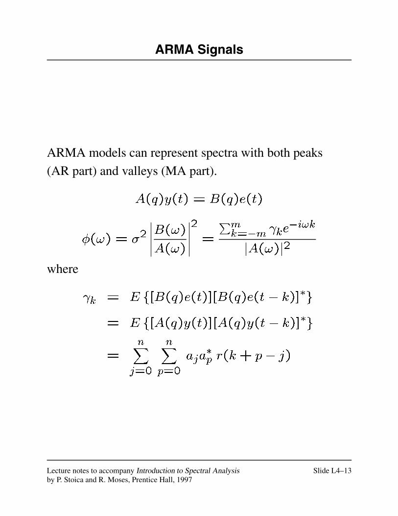
ARMA Signals

ARMA models can represent spectra with both peaks

(AR part) and valleys (MA part).

A(q)y(t) = B(q)e(t)

�(!) = �2��B(!)A(!)

��2

=

Pmk=�m ke

�i!k

jA(!)j2

where

k = E f[B(q)e(t)][B(q)e(t � k)]�g

= E f[A(q)y(t)][A(q)y(t � k)]�g

=nX

j=0

nXp=0

aja�p r(k+ p� j)


ARMA Spectrum Estimation

Two Methods:

1. Estimate fai; bj; �2g in �(!) = �2��B(!)A(!)

��2

� nonlinear estimation problem; can use an approximate

linear two-stage least squares method

� �(!) is guaranteed to be� 0

2. Estimate fai; r(k)g in �(!) =Pm

k=�m ke�i!k

jA(!)j2

� linear estimation problem (the Modified Yule-Walker

method).

� �(!) is not guaranteed to be� 0


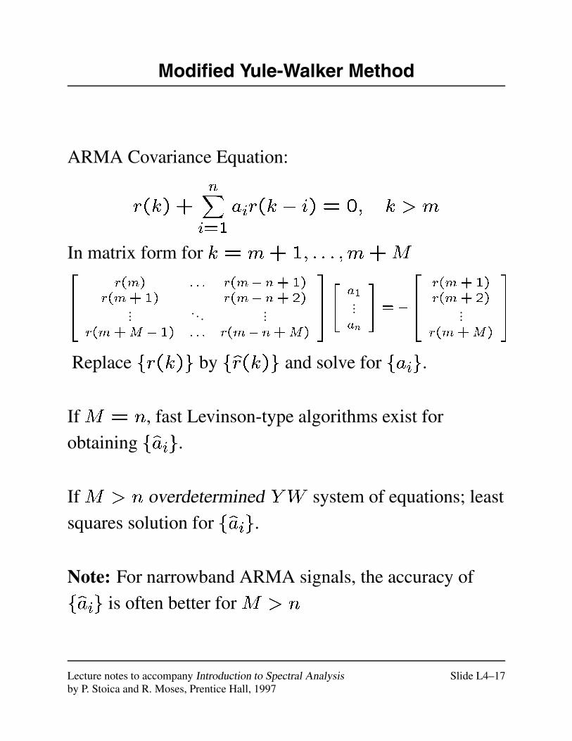
Modified Yule-Walker Method

ARMA Covariance Equation:

r(k) +nXi=1

air(k � i) = 0; k > m

In matrix form for k = m+1; : : : ;m+M264

r(m) : : : r(m� n+1)r(m+1) r(m� n+2)

... . . . ...r(m+M � 1) : : : r(m� n+M)

375"

a1...an

#= �

264

r(m+1)r(m+2)

...r(m+M)

375

Replace fr(k)g by fr(k)g and solve for faig.

If M = n, fast Levinson-type algorithms exist for

obtaining faig.

If M > n overdetermined YW system of equations; least

squares solution for faig.

Note: For narrowband ARMA signals, the accuracy of

faig is often better for M > n


Su

mm

ary

of

Par

amet

ric

Met

ho

ds

for

Rat

ion

alS

pec

tra

Com

puta

tiona

lG

uara

ntee

Met

hod

Bur

den

Acc

urac

y

^ �(!)�

0

?U

sefo

rA

R:Y

Wor

LS

low

med

ium

Yes

Spec

tra

with

(nar

row

)pe

aks

but

nova

lley

MA

:BT

low

low

-med

ium

No

Bro

adba

ndsp

ectr

apo

ssib

lyw

ithva

lleys

butn

ope

aks

AR

MA

:MY

Wlo

w-m

ediu

mm

ediu

mN

oSp

ectr

aw

ithbo

thpe

aks

and

(not

too

deep

)va

lleys

AR

MA

:2-S

tage

LS

med

ium

-hig

hm

ediu

m-h

igh

Yes

As

abov

e

Lec

ture

note

sto

acco

mpa

nyIn

trod

uctio

nto

Spec

tral

Ana

lysi

sSl

ide

L4–

18by

P.St

oica

and

R.M

oses

,Pre

ntic

eH

all,

1997

Parametric Methods

for

Line Spectra — Part 1

Lecture 5


Line Spectra

Many applications have signals with (near) sinusoidalcomponents. Examples:

� communications

� radar, sonar

� geophysical seismology

ARMA model is a poor approximation

Better approximation by Discrete/Line Spectrum Models

-

6

6

6

6

�2

�� !1 !2 !3

(2��21)(2��22)

(2��23)

!

�(!)

An “Ideal” line spectrum


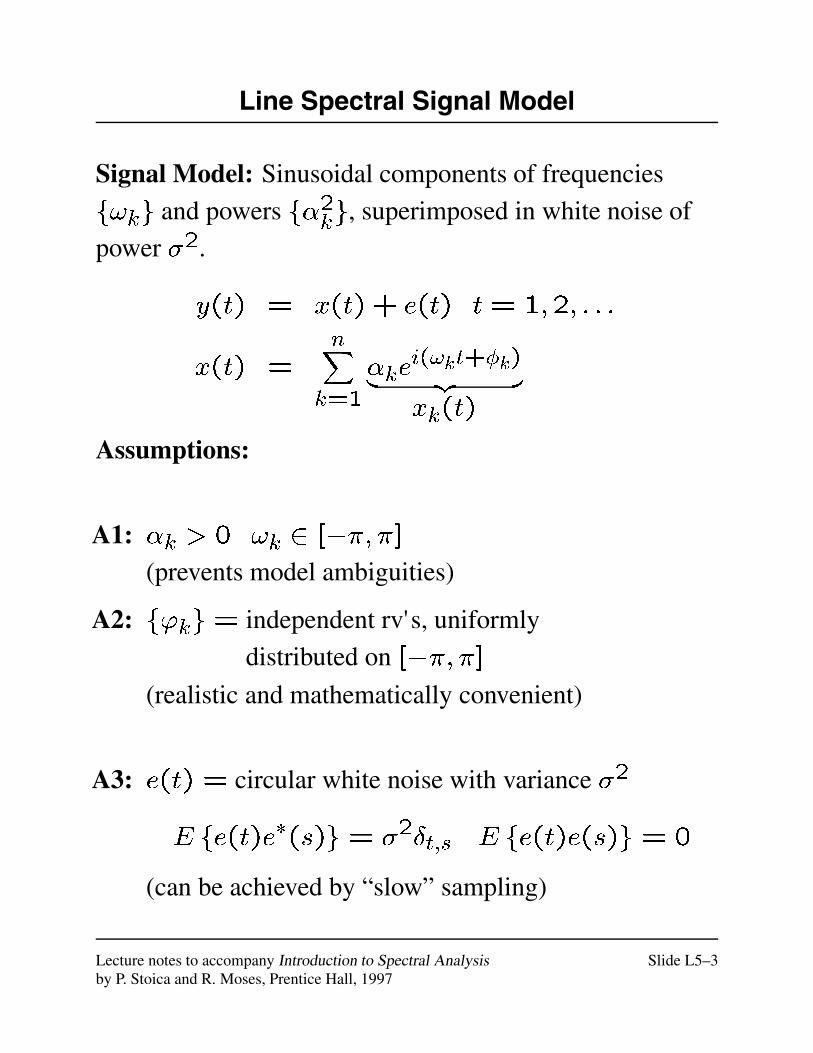
Line Spectral Signal Model

Signal Model: Sinusoidal components of frequencies

f!kg and powers f�2kg, superimposed in white noise of

power �2.

y(t) = x(t) + e(t) t = 1;2; : : :

x(t) =nX

k=1

�kei(!kt+�k)| {z }xk(t)

Assumptions:

A1: �k > 0 !k 2 [��; �]

(prevents model ambiguities)

A2: f'kg= independent rv's, uniformly

distributed on [��; �]

(realistic and mathematically convenient)

A3: e(t) = circular white noise with variance �2

E fe(t)e�(s)g = �2�t;s E fe(t)e(s)g = 0

(can be achieved by “slow” sampling)


Covariance Function and PSD

Note that:

� Enei'pe�i'j

o= 1, for p = j

� Enei'pe�i'j

o= E

nei'p

oEne�i'j

o=

�� 12�Z ��

ei' d'

��2 = 0, for p 6= j

Hence,

Enxp(t)x

�j(t� k)

o= �2p e

i!pk �p;j

r(k) = E fy(t)y�(t� k)g

=Pnp=1�

2pei!pk+ �2�k;0

and

�(!) = 2�nX

p=1

�2p�(! � !p) + �2


Parameter Estimation

Estimate either:

� f!k; �k; 'kgnk=1; �

2 (Signal Model)

� f!k; �2kgnk=1; �

2 (PSD Model)

Major Estimation Problem: f!kg

Once f!kg are determined:

� f�2kg can be obtained by a least squares method from

r(k) =nX

p=1

�2pei!pk + residuals

OR:

� Both f�kg and f'kg can be derived by a leastsquares method from

y(t) =nX

k=1

�kei!kt + residuals

with �k = �kei'k .


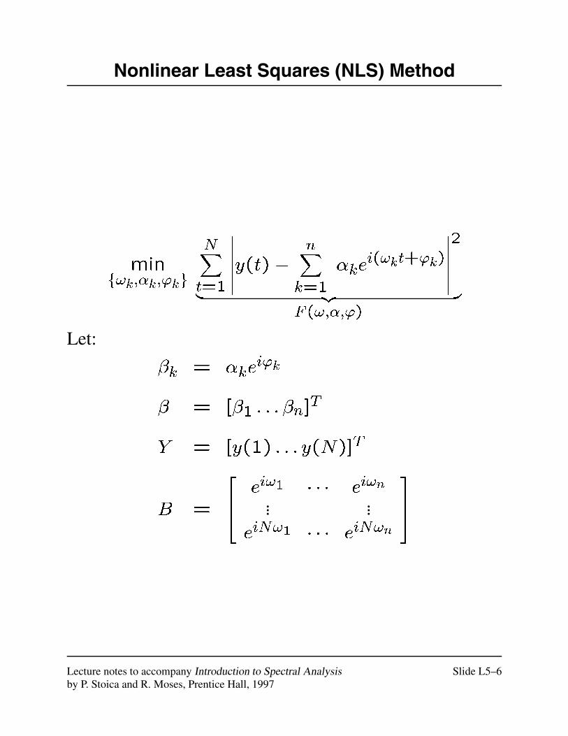
Nonlinear Least Squares (NLS) Method

minf!k;�k;'kg

NXt=1

��y(t)�nX

k=1

�kei(!kt+'k)

��2

| {z }F(!;�;')

Let:

�k = �kei'k

� = [�1 : : : �n]T

Y = [y(1) : : : y(N)]T

B =

264 ei!1 � � � ei!n

... ...eiN!1 � � � eiN!n

375


Nonlinear Least Squares (NLS) Method, con't

Then:

F = (Y �B�)�(Y �B�) = kY �B�k2

= [� � (B�B)�1B�Y ]�[B�B]

[� � (B�B)�1B�Y ]

+Y �Y � Y �B(B�B)�1B�Y

This gives:

� = (B�B)�1B�Y��!=!

and

! = arg max!

Y �B(B�B)�1B�Y


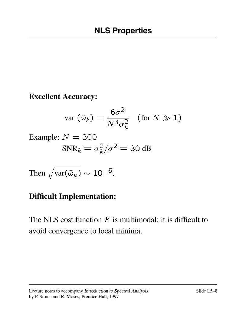
NLS Properties

Excellent Accuracy:

var (!k) =6�2

N3�2k(for N � 1)

Example: N = 300

SNRk = �2k=�2 = 30 dB

Thenq

var(!k) � 10�5.

Difficult Implementation:

The NLS cost function F is multimodal; it is difficult to

avoid convergence to local minima.


Parametric Methods

for

Line Spectra — Part 2

Lecture 6


The Covariance Matrix Equation

Let:

a(!) = [1 e�i! : : : e�i(m�1)!]T

A = [a(!1) : : : a(!n)] (m� n)

Note: rank(A) = n (for m � n )

Define

~y(t)4=

26664

y(t)y(t� 1)

...y(t�m+1)

37775 = A~x(t) + ~e(t)

where

~x(t) = [x1(t) : : : xn(t)]T

~e(t) = [e(t) : : : e(t�m+1)]T

Then

R4= E f~y(t)~y�(t)g = APA�+ �2I

with

P = E f~x(t)~x�(t)g =

264 �

21 0

. . .0 �2n

375


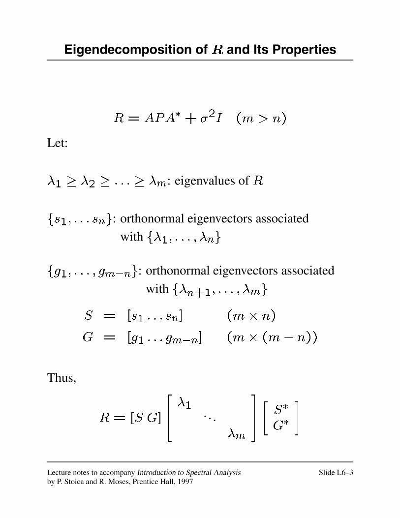
Eigendecomposition of R and Its Properties

R = APA�+ �2I (m > n)

Let:

�1 � �2 � : : : � �m: eigenvalues of R

fs1; : : : sng: orthonormal eigenvectors associated

with f�1; : : : ; �ng

fg1; : : : ; gm�ng: orthonormal eigenvectors associated

with f�n+1; : : : ; �mg

S = [s1 : : : sn] (m� n)

G = [g1 : : : gm�n] (m� (m� n))

Thus,

R = [S G]

264 �1 . . .

�m

375"S�

G�

#


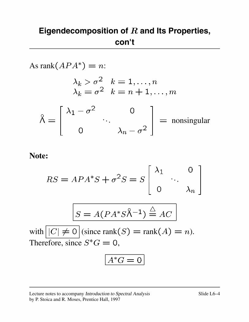
Eigendecomposition of R and Its Properties,con't

As rank(APA�) = n:

�k > �2 k = 1; : : : ; n

�k = �2 k = n+1; : : : ;m

��=

264 �1 � �

2 0. . .

0 �n � �2

375 = nonsingular

Note:

RS = APA�S+ �2S = S

264 �1 0

. . .0 �n

375

S = A(PA�S�� 1)

4= AC

with jCj 6= 0 (since rank(S) = rank(A) = n).

Therefore, since S�G= 0,

A�G = 0


MUSIC Method

A�G=

264 a

�(!1)...

a�(!n)

375 G = 0

) fa(!k)gnk=1 ? R(G)

Thus,

f!kgnk=1 are the unique solutions of

a�(!)GG�a(!) = 0.

Let:

R =1

N

NXt=m

~y(t)~y�(t)

S; G = S;G made from the

eigenvectors of R


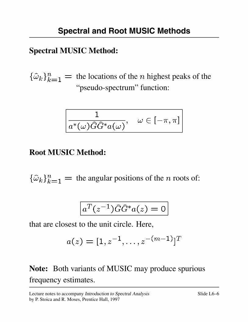
Spectral and Root MUSIC Methods

Spectral MUSIC Method:

f!kgnk=1 = the locations of the n highest peaks of the

“pseudo-spectrum” function:

1

a�(!)GG�a(!); ! 2 [��; �]

Root MUSIC Method:

f!kgnk=1 = the angular positions of the n roots of:

aT (z�1)GG�a(z) = 0

that are closest to the unit circle. Here,

a(z) = [1; z�1; : : : ; z�(m�1)]T

Note: Both variants of MUSIC may produce spuriousfrequency estimates.


Spatial Methods — Part 1

Lecture 8


The Spatial Spectral Estimation Problem

Source n

Source 2Source 1

�

BBBBBN

@@@@R

v

v

v

Sensor 1

@@ ��

@@ ��

@@ ��

Sensor 2

Sensor m

ccccc

cccc

ccc

��,

,,

,,

,,,

,,

,,

Problem: Detect and locate n radiating sources by using

an array of m passive sensors.

Emitted energy: Acoustic, electromagnetic, mechanical

Receiving sensors: Hydrophones, antennas, seismometers

Applications: Radar, sonar, communications, seismology,

underwater surveillance

Basic Approach: Determine energy distribution over

space (thus the name “spatial spectral analysis”)


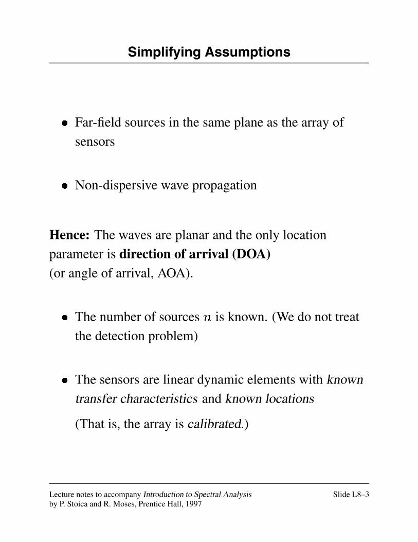
Simplifying Assumptions

� Far-field sources in the same plane as the array of

sensors

� Non-dispersive wave propagation

Hence: The waves are planar and the only location

parameter is direction of arrival (DOA)(or angle of arrival, AOA).

� The number of sources n is known. (We do not treat

the detection problem)

� The sensors are linear dynamic elements with knowntransfer characteristics and known locations

(That is, the array is calibrated.)


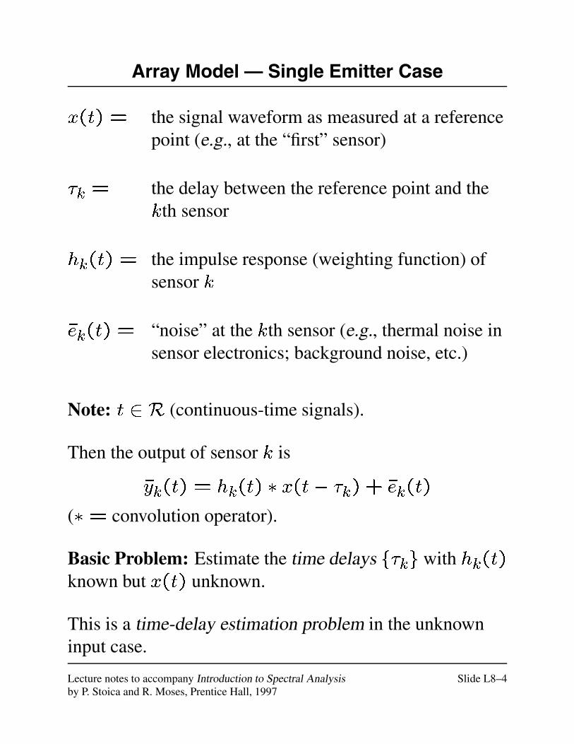
Array Model — Single Emitter Case

x(t) = the signal waveform as measured at a referencepoint (e.g., at the “first” sensor)

�k = the delay between the reference point and thekth sensor

hk(t) = the impulse response (weighting function) ofsensor k

�ek(t) = “noise” at the kth sensor (e.g., thermal noise insensor electronics; background noise, etc.)

Note: t 2 R (continuous-time signals).

Then the output of sensor k is

�yk(t) = hk(t) � x(t� �k) + �ek(t)

(� = convolution operator).

Basic Problem: Estimate the time delays f�kg with hk(t)known but x(t) unknown.

This is a time-delay estimation problem in the unknowninput case.


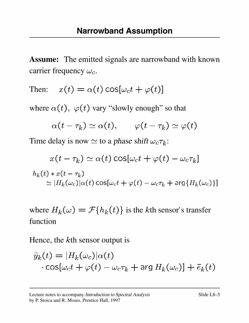
Narrowband Assumption

Assume: The emitted signals are narrowband with known

carrier frequency !c.

Then: x(t) = �(t) cos[!ct+ '(t)]

where �(t); '(t) vary “slowly enough” so that

�(t� �k) ' �(t); '(t� �k) ' '(t)

Time delay is now' to a phase shift !c�k:

x(t� �k) ' �(t) cos[!ct+ '(t)� !c�k]

hk(t) � x(t� �k)

' jHk(!c)j�(t) cos[!ct+ '(t)� !c�k +argfHk(!c)g]

where Hk(!) = Ffhk(t)g is the kth sensor's transfer

function

Hence, the kth sensor output is

�yk(t) = jHk(!c)j�(t)

� cos[!ct+ '(t)� !c�k+ argHk(!c)] + �ek(t)


Complex Signal Representation

The noise-free output has the form:

z(t) = �(t) cos [!ct+ (t)] =

=�(t)

2

nei[!ct+ (t)]+ e�i[!ct+ (t)]

oDemodulate z(t) (translate to baseband):

2z(t)e�!ct = �(t)f ei (t)| {z }lowpass

+ e�i[2!ct+ (t)]| {z }highpass

g

Lowpass filter 2z(t)e�i!ct to obtain �(t)ei (t)

Hence, by low-pass filtering and sampling the signal

~yk(t)=2 = �yk(t)e�i!ct

= �yk(t) cos(!ct)� i�yk(t) sin(!ct)

we get the complex representation: (for t 2 Z)

yk(t) = �(t) ei'(t)| {z }s(t)

jHk(!c)j eiarg[Hk(!c)]| {z }

Hk(!c)

e�i!c�k + ek(t)

or

yk(t) = s(t)Hk(!c) e�i!c�k + ek(t)

where s(t) is the complex envelope of x(t).


Vector Representation for a Narrowband Source

Let

� = the emitter DOA

m = the number of sensors

a(�) =

264 H1(!c) e

�i!c�1...

Hm(!c) e�i!c�m

375

y(t) =

264 y1(t)

...ym(t)

375 e(t) =

264 e1(t)

...em(t)

375

Then

y(t) = a(�)s(t) + e(t)

NOTE: � enters a(�) via both f�kg and fHk(!c)g.

For omnidirectional sensors the fHk(!c)g do not depend

on �.


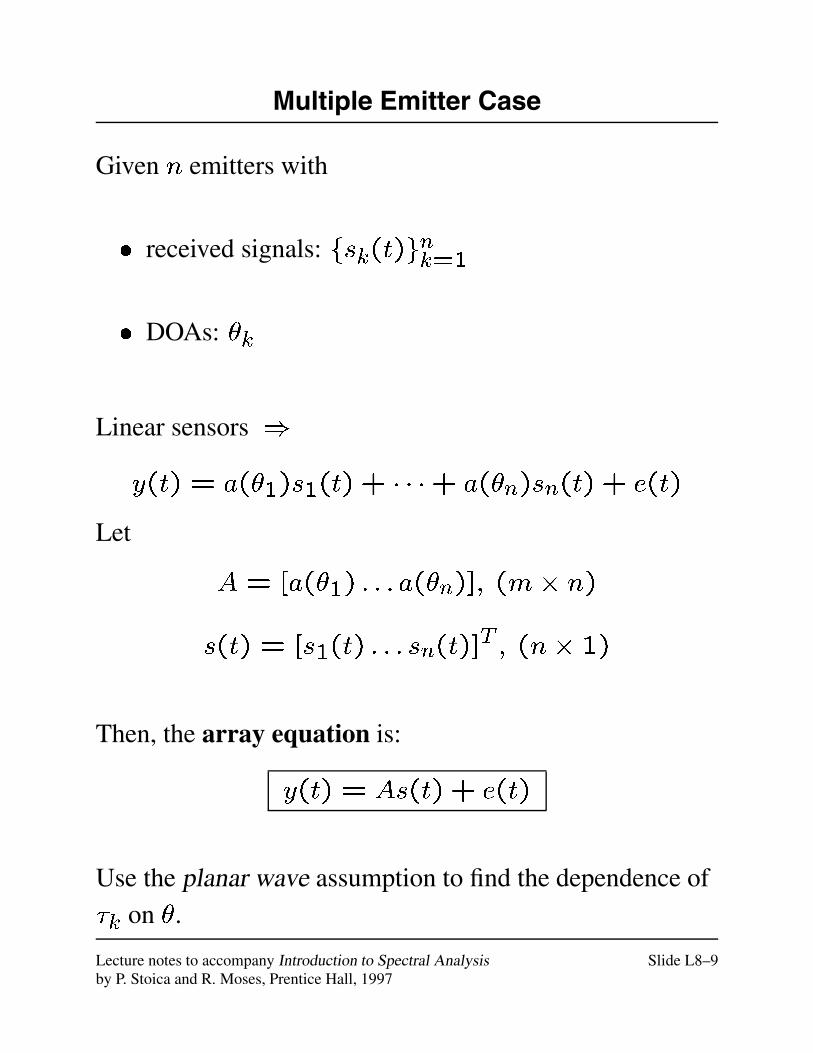
Multiple Emitter Case

Given n emitters with

� received signals: fsk(t)gnk=1

� DOAs: �k

Linear sensors )

y(t) = a(�1)s1(t) + � � �+ a(�n)sn(t) + e(t)

Let

A = [a(�1) : : : a(�n)]; (m� n)

s(t) = [s1(t) : : : sn(t)]T ; (n� 1)

Then, the array equation is:

y(t) = As(t) + e(t)

Use the planar wave assumption to find the dependence of�k on �.


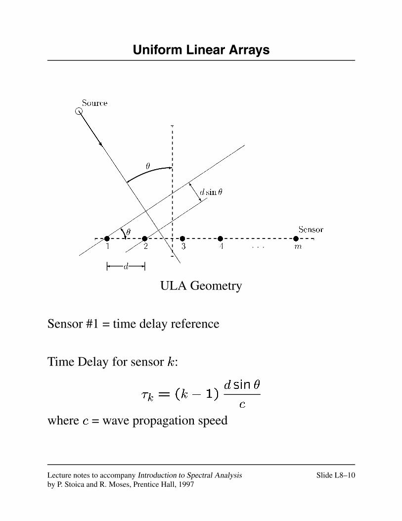
Uniform Linear Arrays

��

Source

-

+

�

?]�

p p p

Sensor

m4321

d sin �JJJJ]

d -�

��

JJJJJJJJJJJJJJJJJJJJJ

JJJJJ

h

v v v v v

ULA Geometry

Sensor #1 = time delay reference

Time Delay for sensor k:

�k = (k � 1)d sin �

c

where c = wave propagation speed


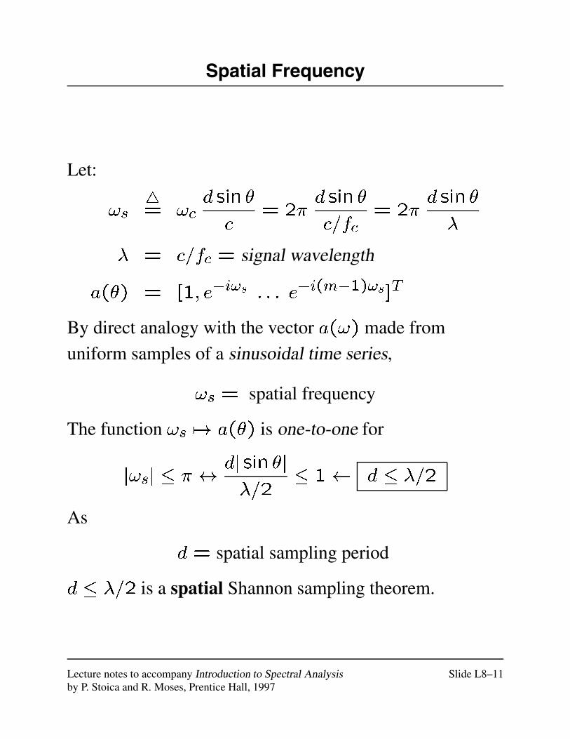
Spatial Frequency

Let:

!s4= !c

d sin �

c= 2�

d sin �

c=fc= 2�

d sin �

�

� = c=fc = signal wavelength

a(�) = [1; e�i!s : : : e�i(m�1)!s]T

By direct analogy with the vector a(!) made from

uniform samples of a sinusoidal time series,

!s = spatial frequency

The function !s 7! a(�) is one-to-one for

j!sj � � $dj sin �j

�=2� 1 d � �=2

As

d = spatial sampling period

d � �=2 is a spatial Shannon sampling theorem.


Spatial Filtering

Spatial filtering useful for

� DOA discrimination (similar to frequency

discrimination of time-series filtering)

� Nonparametric DOA estimation

There is a strong analogy between temporal filtering and

spatial filtering.


Analogy between Temporal and Spatial Filtering

(Temporal sampling)

z

-

qqq

?

?

?

��

-

-

-

-

� ��

� ��

� ��

� ��

@@@@@R

-

?

?

qqq

-s

-

?

s

�

�

�

P

u(t) = ei!t

q�1

q�1

1

m� 1

0BBBBBBBBBBBBBB@

1

e�i!

...

e�i(m�1)!

1CCCCCCCCCCCCCCA

| {z }a(!)

u(t)

h0

h1

hm�1

[h�a(!)]u(t)

(a) Temporal filter

ZZZZZ~

��

��

��

��

narrowband source with DOA=�

(Spatial sampling)

�

�

�

P

z

-

qqq

?

?

?

��

@@@@@R-

-

-

-

� ��

� ��

� ��

� ��

-!!aa

-!!aa

-!!aa

qqq

reference point1

2

m

0BBBBBBBBBBB@

1

e�i!�2(�)

...

e�i!�m(�)

1CCCCCCCCCCCA

| {z }a(�)

s(t)

h0

h1

hm�1

[h�a(�)]s(t)

(b) Spatial filter


Spatial Filtering, con't

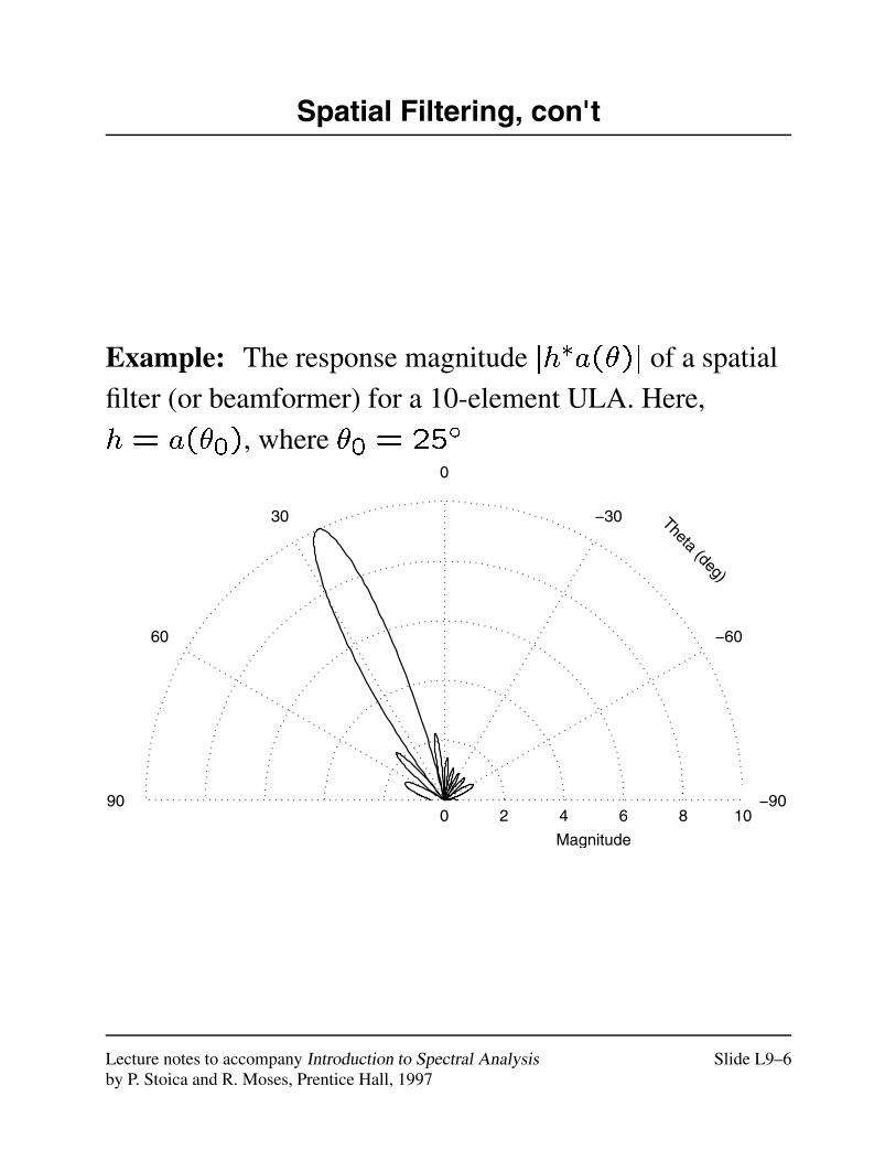
Example: The response magnitude jh�a(�)j of a spatial

filter (or beamformer) for a 10-element ULA. Here,

h = a(�0), where �0 = 25�

2 4 6 8 100

Magnitude

Theta (deg)

−90

−60

−30

0

30

60

90


Spatial Filtering Uses

Spatial Filters can be used

� To pass the signal of interest only, hence filtering out

interferences located outside the filter's beam (but

possibly having the same temporal characteristics as

the signal).

� To locate an emitter in the field of view, by sweeping

the filter through the DOA range of interest

(“goniometer”).


Nonparametric Spatial Methods

A Filter Bank Approach to DOA estimation.

Basic Ideas

� Design a filter h(�) such that for each �

– It passes undistorted the signal with DOA = �

– It attenuates all DOAs 6= �

� Sweep the filter through the DOA range of interest,

and evaluate the powers of the filtered signals:

EnjyF(t)j

2o

= Enjh�(�)y(t)j2

o= h�(�)Rh(�)

with R = E fy(t)y�(t)g.

� The (dominant) peaks of h�(�)Rh(�) give the

DOAs of the sources.


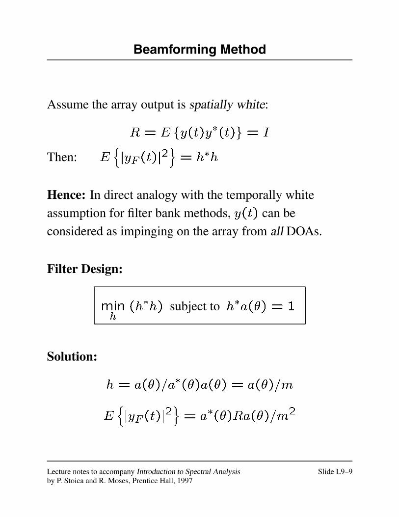
Beamforming Method

Assume the array output is spatially white:

R = E fy(t)y�(t)g = I

Then: EnjyF(t)j

2o= h�h

Hence: In direct analogy with the temporally white

assumption for filter bank methods, y(t) can be

considered as impinging on the array from all DOAs.

Filter Design:

minh

(h�h) subject to h�a(�) = 1

Solution:

h = a(�)=a�(�)a(�) = a(�)=m

EnjyF(t)j

2o= a�(�)Ra(�)=m2


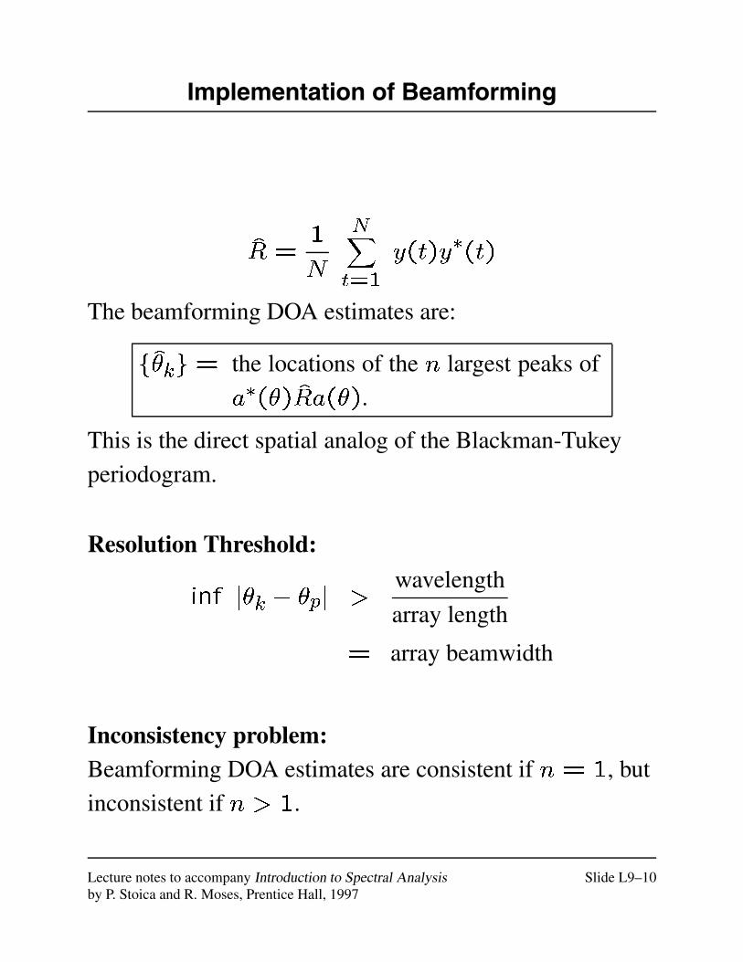
Implementation of Beamforming

R =1

N

NXt=1

y(t)y�(t)

The beamforming DOA estimates are:

f�kg= the locations of the n largest peaks of

a�(�)Ra(�).

This is the direct spatial analog of the Blackman-Tukey

periodogram.

Resolution Threshold:

inf j�k � �pj >wavelength

array length

= array beamwidth

Inconsistency problem:Beamforming DOA estimates are consistent if n= 1, but

inconsistent if n > 1.


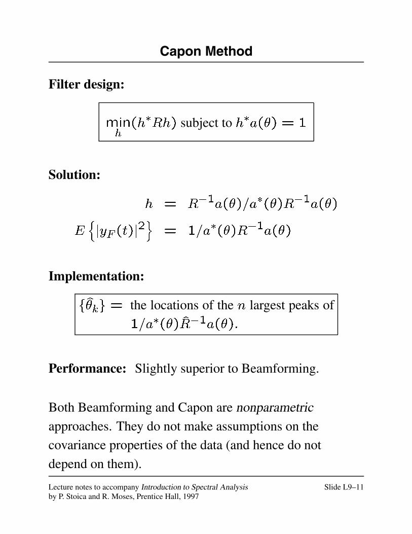
Capon Method

Filter design:

minh(h�Rh) subject to h�a(�) = 1

Solution:

h = R�1a(�)=a�(�)R�1a(�)

EnjyF(t)j

2o

= 1=a�(�)R�1a(�)

Implementation:

f�kg = the locations of the n largest peaks of

1=a�(�)R�1a(�):

Performance: Slightly superior to Beamforming.

Both Beamforming and Capon are nonparametricapproaches. They do not make assumptions on the

covariance properties of the data (and hence do not

depend on them).


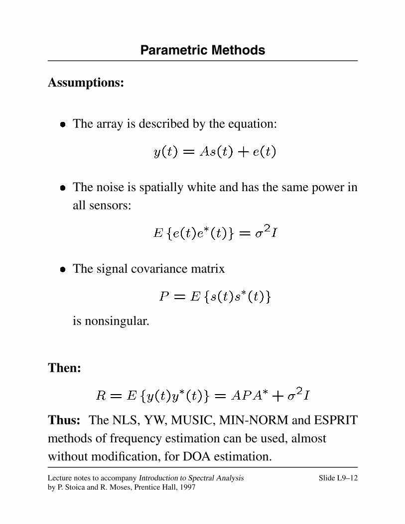
Parametric Methods

Assumptions:

� The array is described by the equation:

y(t) = As(t) + e(t)

� The noise is spatially white and has the same power inall sensors:

E fe(t)e�(t)g = �2I

� The signal covariance matrix

P = E fs(t)s�(t)g

is nonsingular.

Then:

R = E fy(t)y�(t)g = APA�+ �2I

Thus: The NLS, YW, MUSIC, MIN-NORM and ESPRITmethods of frequency estimation can be used, almostwithout modification, for DOA estimation.


periodogram and correlogram methods - tuttabus/course/advsp/21006lectures10_12.pdf · correlogram...

Documents