perspectives on kuperberg flowshomepages.math.uic.edu/~hurder/papers/82manuscriptv2.pdf ·...

PERSPECTIVES ON KUPERBERG FLOWS

STEVEN HURDER AND ANA RECHTMAN

Dedicated to Professor Krystyna Kuperberg on the occasion of her 70th birthday

Abstract. The “Seifert Conjecture” stated, “Every non-singular vector field on the 3-sphere S3 has a

periodic orbit”. In a celebrated work, Krystyna Kuperberg gave a construction of a smooth aperiodic vector

field on a plug, which is then used to construct counter-examples to the Seifert Conjecture for smooth flowson the 3-sphere, and on compact 3-manifolds in general. The dynamics of the flows in these plugs have been

extensively studied, with more precise results known in special “generic” cases of the construction. Moreover,the dynamical properties of smooth perturbations of Kuperberg’s construction have been considered. In this

work, we recall some of the results obtained to date for the Kuperberg flows and their perturbations. Then

the main point of this work is to focus attention on how the known results for Kuperberg flows depend onthe assumptions imposed on the flows, and to discuss some of the many interesting questions and problems

that remain open about their dynamical and ergodic properties.

Contents

1. Introduction 2

2. Modified Wilson plugs 5

3. The Kuperberg plugs 8

4. Generic hypotheses 12

5. Wandering and minimal sets 15

6. Zippered laminations 17

7. Denjoy Theory for laminations 19

8. Growth, slow entropy, and Hausdorff dimension 21

9. Shape theory for the minimal set 24

10. Derived from Kuperberg flows 27

References 29

Preprint date: October 21, 2016; revised July 10, 2017.

2010 Mathematics Subject Classification. Primary 37C10, 37C70, 37B40, 37B45; Secondary 37D45, 57R30, 58H05.

1

2 STEVEN HURDER AND ANA RECHTMAN

1. Introduction

In his 1950 work [59], Seifert introduced an invariant for deformations of non-singular flows with a closedorbit on a 3-manifold, which he used to show that every sufficiently small deformation of the Hopf flow onthe 3-sphere S3 must have a closed orbit. He also remarked in Section 5 of this work:

It is unknown if every continuous (non-singular) vector field on the three-dimensional spherecontains a closed integral curve.

This remark became the basis for what is known as the “Seifert Conjecture”:

Every non-singular vector field on the 3-sphere S3 has a periodic orbit.

The Seminaire Bourbaki article [22] by Ghys discusses the background and obstacles to the construction ofaperiodic flows in 3-dimensions. We recall some of the key developments.

In his 1966 work [67], and see also [53], Wilson showed that every closed 3-manifold M has a flow withonly finitely many closed orbits. The Seifert Conjecture was thus reduced to showing that given a flow on a3-manifold with only a finite number of periodic orbits, it can be modified to one with no periodic orbits.

Wilson introduced the notion of a “plug” for a flow on M , which is a neighborhood P ⊂ M diffeomorphicto a disk cross an interval, P ∼= D2 × [−1, 1], where orbits enter one end of the plug, ∂−P = D2 × −1,and exit the other end, ∂+P = D2 × +1. Wilson showed how to modify the flow inside a plug so that itcontains exactly two closed orbits. These Wilson plugs are used to modify a given non-singular flow on aclosed 3-manifold, to obtain one with only isolated periodic orbits.

In his 1974 work [58], Schweitzer gave a modification of the construction of the Wilson plug, replacingthe periodic orbits in the plug with invariant Denjoy-type minimal sets for the modified flow in the plug, toobtain a C1-flow with no periodic orbits. He used this plug to show that there exists a non-singular C1-vectorfield without periodic orbits on any closed orientable 3-manifold M . In her 1988 work [26], Harrison gave amodification of the construction of the Schweitzer plug, which yielded an aperiodic plug with a C2-flow.

The Seifert Conjecture was settled for all degrees of smoothness by Krystyna Kuperberg in 1994:

THEOREM 1.1 (Kuperberg [39]). On every closed oriented 3-manifold M , there exists a C∞ non-vanishing vector field without periodic orbits.

Kuperberg introduced a construction of aperiodic 3-dimensional plugs which was notable for its simplicityand beauty, and remains the only general method to date to construct C∞-flows without periodic orbits.

Following Kuperberg’s original work, there was a sequence of three works explaining in further detail thedynamical properties for the Kuperberg flows:

• the Seminaire Bourbaki lecture [22] by Etienne Ghys;• the notes by Shigenori Matsumoto [45];• the joint paper [40] by Greg and Krystyna Kuperberg.

Also, a brief overview of the construction was given in [42]. These works showed that a Kuperberg flow:

• has zero topological entropy, which follows by an observation of Ghys in [22] that an aperiodic flowon a 3-manifold has topological entropy equal to zero, as a consequence of a result of Katok in [36];

• has a unique minimal set Σ, whose topological structure is unknown in general;• has an open set of non-recurrent points that limit on its minimal set Σ, a result of Matsumoto [45];• preserves a 2-dimensional compact lamination M with boundary, that is contained in the interior of

the plug and contains the minimal set Σ.

The two minimal sets for the Wilson flow are each a closed circle, and the two minimal sets for the Schweitzerplug are each homeomorphic to a Denjoy minimal set in the 2-torus. In contrast, the topological type of theunique minimal set Σ for a Kuperberg flow is extraordinarily complicated, and requires further study.

PERSPECTIVES ON KUPERBERG FLOWS 3

Moreover, there are many choices made in the construction of the flows in the Kuperberg plugs, any of whichmay strongly influence their global dynamics. In his survey [22, page 302], Ghys wrote:

Par ailleurs, on peut construire beaucoup de pieges de Kuperberg et il n’est pas clair qu’ilsaient le meme dynamique.

One of the goals of this paper is to bring into focus some of the dynamical properties of Kuperberg flowswhich depend on imposing additional hypotheses in their construction. For example, the monograph [29]introduced the notion of a generic Kuperberg plug, as recalled in Section 4 below. It was shown in [29] thatfor a generic Kuperberg flow, the minimal set Σ is equal to the lamination M. A detailed analysis of thedynamical and topological structure of M was used to give a geometric proof that the topological entropyof the generic Kuperberg flow is zero, and also to show that M has unstable shape.

The statement by Seifert quoted above can be given alternate interpretations as well. For example, one is tofind conditions on a smooth flow on a closed 3-manifold which guarantees the existence of a periodic orbit.It has been shown by Hofer in [27], that the flow of a Reeb vector field on S3 must have a periodic orbit.More generally, Taubes showed in [63] that the flow of a Reeb vector field on a closed 3-manifold has periodicorbits. This theorem was extended to geodesible volume preserving flows (also known as Reeb vector fieldof stable hamiltonian structures) to manifolds that are not torus bundles over the circle by Hutchings andTaubes [33, 34], and Rechtman [49], and for real analytic geodesible flows by Rechtman [57]. The existenceof a periodic orbit is also established for real analytic solutions of the Euler equation by Etnyre and Ghrist[17]. Frankel proved that quasi-geodesic flows on hyperbolic 3-manifolds always have periodic orbits [19].

Another interpretation of Seifert’s work is to ask about the dynamical properties of flows which are closeto an aperiodic flow. For example, the work [30] by the authors constructs smooth families of variations ofthe Kuperberg flow which are not aperiodic, and have invariant horseshoes in their dynamics. We also showthat there are smooth families of variations of the Kuperberg plug with simple dynamics and exactly twoperiodic orbits, but the limit of the family is an aperiodic flow. In such a family, the period of the periodicorbits blows up at the limit. Palis and Shub in [50] asked whether this dynamical phenomenon can occur infamilies of smooth flows on closed manifolds, and called a closed orbit whose length “blows up” to infinityunder deformation a “blue sky catastrophe”. The first examples of a family of flows with this property wasfound by Medvedev in [47]. The constructions in [30] show that deformations of Kuperberg flows provide anew class of examples. The work of A. Shilnikov, L. Shilnikov and D. Turaev in [60] gives a discussion ofstronger formulations of the blue sky catastrophe phenomenon.

Thus, Kuperberg flows are special in that they are aperiodic, have many further special dynamical propertiesand lie at the “boundary of chaos” in the C∞-topology on flows. These properties suggest topics for furtherstudy, and this is the theme of this survey:

There are many interesting open problems concerning Kuperberg flows!

We first describe the construction of the Kuperberg plugs. Section 2 gives the construction of the modifiedWilson plugs, which provides the foundation of the construction. Section 3 then gives the construction ofthe Kuperberg plugs. These constructions are given in a succinct manner, and the interested reader canconsult the literature cited above for further details and discussions.

Section 4 introduces the generic hypotheses for the Kuperberg construction, as given in the works [29, 30].We also introduce variations of these generic hypotheses, whose implications for the dynamics of the flowswill be discussed in later sections.

It was observed in the works [22, 45] that any orbit not escaping the plug in forward or backward time,limits to the invariant set defined as the closure of the “special orbits” for the flow. One consequence is thatthe Kuperberg flow has a unique minimal set in the plug, denoted by Σ, as recalled in Theorem 5.1.

A remarkable aspect of the construction of a Kuperberg flow is that it preserves an embedded infinite surfacewith boundary, denoted by M0. The boundary of M contains the special orbits, and so its closure M = M0

is a type of lamination with boundary that contains the minimal set Σ. The relation between the two setsΣ ⊂M is an important theme in the study of the dynamics of Kuperberg flows. Section 6 gives an outline


of the structure theory for the embedded surface M0 in the case of generic flows, as developed in [29]. Thisstructure theory, and the corresponding properties of the level function defined on M0, are crucial for theproofs in [29].

In Section 7, we develop conditions on a flow which are sufficient to show that the inclusion of the minimalset Σ in the laminated space M is an equality. This result is a type of “Denjoy Theorem” for laminations,and its proof in [29] relies on the generic hypotheses for the flow in fundamental ways. It is an interestingproblem whether this is a special case of a more general formulation of a Denjoy Theorem for laminations,which we present here as it is independent of the development of Kuperberg flows.

PROBLEM (Problem 7.9). Let L be a compact, connected 2-dimensional lamination which is embedded ina compact 3-manifold M , and let X be a smooth vector field tangent to the leaves of L. Suppose that thelamination L is minimal, that is, every 2-dimensional leaf of L is dense in L. Also assume that the flow ofX has no periodic orbits. Show that every orbit of X is dense in L.

Ghys observed in [22] that an aperiodic flow must have entropy equal to zero, using a well-known result ofKatok [36], and thus a Kuperberg flow restricted to the lamination M must have zero entropy. The authorsshowed in [29], that while the usual entropy of the flow vanishes, the “slow entropy” as defined in [9, 37] of ageneric Kuperberg flow is positive for exponent α = 1/2. This calculation used two special properties of theKuperberg construction. One is that the embedded surface M0 ⊂ K has subexponential but not polynomialgrowth rate, which follows from the structure theory developed for M0 in the generic case. The second isthat the surface M0 is the union of two infinite surfaces, corresponding to the two insertion maps used in theconstruction of the plug, and the flow along these surfaces separates points when they encounter the upperand lower insertions. It is an interesting problem to study the entropy-like invariants for all Kuperberg flows,not just the generic flows. Analogously, it is important to estimate the Hausdorff dimensions of the sets Σand M, and how they depend on the choices used in the construction of the Kuperberg flow. These andrelated questions are addressed in Section 8.

A standard problem in topological dynamical systems theory is to describe the topological type of the closedattractors for the system, and for closed invariant transitive subsets more generally. Attractors often havevery complicated topological description, and the theory of shape for spaces [43, 44] is used to describe them.Describing the shape of a dynamically defined invariant set of an arbitrary flow is typically quite difficult,but also can be highly revealing about the dynamical properties of the flow.

In Section 9, we discuss the shape properties of the unique minimal set for Kuperberg flows. For a genericKuperberg flow, the shape of the minimal set Σ was shown in [29] to be not stable, as defined in Definition 9.3,but to satisfy a Mittag-Leffler Property on its homology groups, as defined in Proposition 9.10. The proofsof these assertions require the structure theory for the invariant set M, and a key idea is the construction ofshape approximations to M using its level hierarchy, as developed in the monograph [29].

The construction of shape approximations of the minimal set Σ suggests a relationship between the entropy ofthe flow and its shape properties. The following problem can be stated for general flows, and the motivationis given in Section 9 and Problem 9.8.

PROBLEM. Assume that a flow of a closed 3-manifold M has an exceptional minimal set Σ whose shapeis not stable. Is the slow entropy of the flow positive?

Recall that a minimal set is said to be exceptional if it is not a submanifold of the ambient manifold M . WhenM has low dimension, this implies that the minimal set has “small” dimension, that is it has dimension 1or 2. The assumption that the shape of Σ is not stable implies that the topological type of its shapeapproximations keep changing as they become increasingly fine, while the assumption that every orbit of theflow in Σ is dense implies a type of recurrence for the topology of the shape approximations. The problem isthen asking if these assumptions are sufficient to guarantee that the topological type of the approximationsexhibit a form of self-similarity in their topological type, which implies that there are exponential separationof the points in the orbit of the flow, at some possibly subexponential rate, as for Kuperberg flows.


Section 10 discusses a variety of questions about the flows which are C∞-close to Kuperberg flows. TheDerived from Kuperberg flows, or DK–flows, were introduced in [30], and are obtained by varying the con-struction of the usual Kuperberg flows, to obtain smooth families of flows containing Kuperberg flows, so areof central interest from the point of view of the properties of Kuperberg flows in the space of flows. The work[30] gave constructions of DK–flows which in fact have countably many independent horseshoe subsystems,and thus have positive topological entropy. Moreover, these examples can be constructed arbitrarily closeto the generic Kuperberg flows. It is notable that the horseshoes generated by a variation of the Kuper-berg construction are shown to exist using the shape approximations discussed in Section 9, providing morereasons to explore the relation between shape and entropy for flows.

It seems a good moment to comment on a question related to volume preserving flows on 3-manifolds. Thereare examples with a finite number of periodic orbits and C1 examples without periodic orbits on any closed3-manifold. These were constructed in [41] by Greg Kuperberg using plugs. Is it possible to build a C∞

volume preserving aperiodic plug? Can we a priori say something about its minimal and invariant sets?

The authors dedicate this work to Krystyna Kuperberg for her discovery of the class of dynamical systemsintroduced in her celebrated works on aperiodic flows. We are grateful for her comments and suggestions tothe authors that have inspired our continued fascination with “Kuperberg flows”.

2. Modified Wilson plugs

In this section, we present the construction of the Wilson plugs which are the foundation for the constructionof the Kuperberg plugs, with commentary on the choices made. First, we recall that a “plug” is a manifoldwith boundary endowed with a flow, that enables the modification of a given flow on a 3-manifold inside aflow-box. The idea is that after modification by insertion of a plug, a periodic orbit for the given flow is“broken open” – it enters the plug and never exits. Moreover, Kuperberg’s construction does this modificationwithout introducing additional periodic orbits. The first step is to construct Kuperberg’s modified Wilsonplug, which is analogous to the modified Wilson plug used by Schweitzer in [58].

The notion of a “plug” to be inserted in a flow on a 3-manifold was introduced by Wilson [67, 53]. A3-dimensional plug is a manifold P endowed with a vector field X satisfying the following conditions. The3-manifold P is of the form D × [−2, 2], where D is a compact 2-manifold with boundary ∂D. Set

∂vP = ∂D × [−2, 2] , ∂−h P = D × −2 , ∂+h P = D × 2 .Then the boundary of P has a decomposition

∂P = ∂vP ∪ ∂hP = ∂vP ∪ ∂−h P ∪ ∂+h P .

Let ∂∂z be the vertical vector field on P , where z is the coordinate of the interval [−2, 2].

The vector field X must satisfy the conditions:

(P1) vertical at the boundary : X = ∂∂z in a neighborhood of ∂P ; thus, ∂−h P and ∂+h P are the entry and

exit regions of P for the flow of X , respectively;(P2) entry-exit condition: if a point (x,−2) is in the same trajectory as (y, 2), then x = y. That is, an

orbit that traverses P , exits just in front of its entry point;(P3) trapped orbit : there is at least one entry point whose entire forward orbit is contained in P ; we will

say that its orbit is trapped by P ;(P4) tame: there is an embedding i : P → R3 that preserves the vertical direction.

Note that conditions (P2) and (P3) imply that if the forward orbit of a point (x,−2) is trapped, then thebackward orbit of (x, 2) is also trapped.

A semi-plug is a manifold P endowed with a vector field X as above, satisfying conditions (P1), (P3) and(P4), but not necessarily (P2). The concatenation of a semi-plug with an inverted copy of it, that is a copywhere the direction of the flow is inverted, is then a plug.

Note that condition (P4) implies that given any open ball B(~x, ε) ⊂ R3 with ε > 0, there exists a modifiedembedding i′ : P → B(~x, ε) which preserves the vertical direction again. Thus, a plug can be used to change


a vector field Z on any 3-manifold M inside a flowbox, as follows. Let ϕ : Ux → (−1, 1)3 be a coordinatechart which maps the vector field Z on M to the vertical vector field ∂

∂z . Choose a modified embedding

i′ : P → B(~x, ε) ⊂ (−1, 1)3, and then replace the flow ∂∂z in the interior of i′(P ) with the image of X . This

results in a flow Z ′ on M .

The entry-exit condition implies that a periodic orbit of Z which meets ∂hP in a non-trapped point, willremain periodic after this modification. An orbit of Z which meets ∂hP in a trapped point never exits theplug P , hence after modification, limits to a closed invariant set contained in P . A closed invariant setcontains a minimal set for the flow, and thus, a plug serves as a device to insert a minimal set into a flow.

In the work of Wilson [67], the basic plug has the shape of a solid cylinder, whose base ∂−h P = D× −2 isa planar disk D2. Schweitzer introduced in [58] plugs for which the base is obtained from a 2-torus minusan open disk, so ∂−h P

∼= T2 − D2, which has the homotopy type of a wedge of two circles. As we shall seebelow, a key idea behind the Kuperberg construction is to consider a base which is obtained from an annulusby adding two connecting strips, so has the homotopy type of three circles. The “modified Wilson Plug” isa flow on a cylinder minus its core. The flow has two periodic orbits, and the dynamics of the flow is notstable under perturbations. The instability of its dynamics is a key property of these modified plugs.

The first step in the construction is to define a flow on a rectangle as follows. The rectangle is defined by

(1) R = [1, 3]× [−2, 2] = (r, z) | 1 ≤ r ≤ 3 &− 2 ≤ z ≤ 2 .

For a constant 0 < g0 ≤ 1, choose a C∞-function g : R → [0, g0] which satisfies the “vertical” symmetrycondition g(r, z) = g(r,−z). Also, require that g(2,−1) = g(2, 1) = 0, that g(r, z) = g0 for (r, z) near theboundary of R, and that g(r, z) > 0 otherwise.

Define the vector fieldWv = g· ∂∂z . Note thatWv has two singularities, at (2,±1), and is otherwise everywherevertical. The flow lines of this vector field are illustrated in Figure 1. The value of g0 chosen influences thequantitative nature of the flow, as small values of g0 result in a slower vertical climb for the flow, but doesnot alter the qualitative nature of the flow.

Figure 1. Vector field Wv

The next step is to suspend the flow of the vector field Wv to obtain a flow on a a manifold with boundary:

(2) W = [1, 3]× S1 × [−2, 2] ∼= R× S1

with cylindrical coordinates x = (r, θ, z). That is, W is a solid cylinder with an open core removed, obtainedby rotating the rectangle R defined in (1), considered as embedded in R3, around the z-axis.

This is done as follows, where we make more precise choices of the suspension flow than given in [39], thoughthese choices do not matter so much. Choose a C∞-function f : R→ [−1, 1] satisfying the conditions:

(W1) f(r,−z) = −f(r, z) [anti-symmetry in z ](W2) f(r, z) = 0 for (r, z) near the boundary of R(W3) f(r, z) ≥ 0 for −2 ≤ z ≤ 0.(W4) f(r, z) ≤ 0 for 0 ≤ z ≤ 2.(W5) f(r, z) = 1 for 5/4 ≤ r ≤ 11/4 and −7/4 ≤ z ≤ −1/4.(W6) f(r, z) = −1 for 5/4 ≤ r ≤ 11/4 and 1/4 ≤ z ≤ 7/4.


Condition (W1) implies that f(r, 0) = 0 for all 1 ≤ r ≤ 3. The other conditions (W2), (W3), and (W4)are assumed in the works [22, 39, 45] while (W5) and (W6) were imposed in [29] in order to facilitate thedescription of the dynamics of the Kuperberg flows, but do not qualitatively change the resulting dynamics.

Extend the functions f and g above to W by setting f(r, θ, z) = f(r, z) and g(r, θ, z) = g(r, z), so that theyare invariant under rotations around the z-axis. The modified Wilson vector field on W is given by

(3) W = g(r, θ, z)∂

∂z+ f(r, θ, z)

∂

∂θ.

Observe that the vector field W is vertical near the boundary of W and horizontal in the periodic orbits.Also, W is tangent to the cylinders r = cst.

Let Ψt denote the flow of W on W. The flow of Ψt restricted to the cylinders r = cst is illustrated(in cylindrical coordinate slices) by the lines in Figures 2 and 3. The flow of Ψt restricted to the cylinderr = 2 in Figure 2(C) is a called the Reeb flow, which Schweitzer remarks in [58] was the inspiration for hisintroduction of this variation on the Wilson plug.

(a) r ≈ 1, 3 (b) r ≈ 2 (c) r = 2

Figure 2. W-orbits on the cylinders r = cst

Figure 3. W-orbits in the cylinder C = r = 2 and in W

We will make reference to the following sets in W:

C ≡ r = 2 [The Full Cylinder ]

R ≡ (2, θ, z) | −1 ≤ z ≤ 1 [The Reeb Cylinder ]

A ≡ z = 0 [The Center Annulus]

Oi ≡ (2, θ, (−1)i) [Periodic Orbits, i=1,2 ]

Note that O1 is the lower boundary circle of the Reeb cylinder R, and O2 is the upper boundary circle.

Let us also recall some of the basic properties of the modified Wilson flow, which follow from the constructionof the vector field W and the conditions (W1) to (W4) on the suspension function f .

Let Rϕ : W→W be rotation by the angle ϕ. That is, Rϕ(r, θ, z) = (r, θ + ϕ, z).


PROPOSITION 2.1. Let Ψt be the flow on W defined above, then:

(1) Rϕ Ψt = Ψt Rϕ for all ϕ and t.(2) The flow Ψt preserves the cylinders r = cst and in particular preserves the cylinders R and C.(3) Oi for i = 1, 2 are the periodic orbits for Ψt.(4) For x = (2, θ,−2), the forward orbit Ψt(x) for t > 0 is trapped.(5) For x = (2, θ, 2), the backward orbit Ψt(x) for t < 0 is trapped.(6) For x = (r, θ, z) with r 6= 2, the orbit Ψt(x) terminates in the top face ∂+hW for some t ≥ 0, and

terminates in ∂−h W for some t ≤ 0.(7) The flow Ψt satisfies the entry-exit condition (P2) for plugs.

The properties of the flow Ψt on W given in Proposition 2.1 are fundamental for showing that the Kuperbergflows constructed in the next section are aperiodic. On the other hand, the study of the further dynamicalproperties of the Kuperberg flows reveals the importance of the behavior of the flow Ψt in open neighborhoodsof the periodic orbits O1 and O2. This behavior depends strongly on the properties of the function g inopen neighborhoods of its vanishing points (2,±1), as will be discussed in later sections. In particular, notethat if the function g is modified in arbitrarily small neighborhoods of the points (2,−1) and (2, 1), so thatg(r, z) > 0 on R, then the resulting flow on W will have no periodic orbits, and no trapped orbits.

3. The Kuperberg plugs

Kuperberg’s construction in [39] of aperiodic smooth flows on plugs introduced a fundamental new idea, thatof “geometric surgery” on the modified Wilson plug W constructed in the previous section, to obtain theKuperberg Plug K as a quotient space, τ : W → K. The essence of the novel strategy behind the aperiodicproperty of Φt is perhaps best described by a quote from the paper by Matsumoto [45]:

We therefore must demolish the two closed orbits in the Wilson Plug beforehand. Butproducing a new plug will take us back to the starting line. The idea of Kuperberg is tolet closed orbits demolish themselves. We set up a trap within enemy lines and watch themsettle their dispute while we take no active part.

There are many choices made in the implementation of this strategy, where all such choices result in aperiodicflows. On the other hand, some of the choices appear to impact the further dynamical properties of theKuperberg flows, as will be discussed later. We indicate in this section these alternate choices, and laterformulate some of the questions which appear to be important for further study. Finally, at the end of thissection, we consider flows on plugs which violate the above strategy, where the traps for the periodic orbitsare purposely not aligned. This results in what we call “Derived from Kuperberg” flows, or simply DK–flowsfor short, which were introduced in the work [30].

The construction of a Kuperberg Plug K begins with the modified Wilson Plug W with vector field Wconstructed in Section 2. The first step is to re-embed the manifold W in R3 as a folded figure-eight, asshown in Figure 4, preserving the vertical direction.

Figure 4. Embedding of Wilson Plug W as a folded figure-eight


The next step is to construct two (partial) insertions of W in itself, so that each periodic orbit of the Wilsonflow is “broken open” by a trapped orbit on the self-insertion.

The construction begins with the choice in the annulus [1, 3] × S1 of two closed regions Li, for i = 1, 2,which are topological disks. Each region has boundary defined by two arcs: for i = 1, 2, α′i is the boundarycontained in the interior of [1, 3] × S1 and αi in the outer boundary contained in the circle r = 3, asdepicted in Figure 5. In the work [29] the choices for these arcs are given more precisely, though for ourdiscussion here this is not as important.

Figure 5. The disks L1 and L2

Consider the closed sets Di ≡ Li× [−2, 2] ⊂W, for i = 1, 2. Note that each Di is homeomorphic to a closed3-ball, that D1 ∩D2 = ∅, and each Di intersects the cylinder C = r = 2 in a rectangle. Label the top andbottom faces of the closed sets Di by

(4) L±1 = L1 × ±2 , L±2 = L2 × ±2 .

The next step is to define insertion maps σi : Di → W, for i = 1, 2, in such a way that the periodic orbitsO1 and O2 for the W-flow intersect σi(L

−i ) in points corresponding to W-trapped points. Consider two

disjoint arcs β′i in the inner boundary circle r = 1 of [1, 3] × S1, also depicted in Figure 5. Now choosea smooth family of orientation preserving diffeomorphisms σi : L

−i → W, i = 1, 2. Extend these maps to

smooth embeddings σi : Di → W, for i = 1, 2, as illustrated on the left-hand-side of Figure 6. We requirethe following conditions for i = 1, 2:

(K1) σi(α′i × z) = β′i × z for all z ∈ [−2, 2], the interior arc α′i is mapped to a boundary arc β′i.

(K2) Di = σi(Di) then D1 ∩ D2 = ∅;(K3) For every x ∈ Li, the image Ii,x ≡ σi(x× [−2, 2]) is an arc contained in a trajectory of W;(K4) σ1(L−1 ) ⊂ z < 0 and σ2(L+

2 ) ⊂ z > 0;(K5) Each slice σi(Li × z) is transverse to the vector field W, for all −2 ≤ z ≤ 2.(K6) Di intersects the periodic orbit Oi and not Oj , for i 6= j.

The “horizontal faces” of the embedded regions Di ⊂W are labeled by

(5) L±1 = σ1(L±1 ) , L±2 = σ2(L±2 ).

Then the above assumptions imply that faces L±1 of the lower insertion region intersect the first periodicorbit O1 and are disjoint from the second periodic orbit O2, while the faces L±2 of the upper region intersectthe second periodic orbit O2 and are disjoint from O1.

The embeddings σi are also required to satisfy two further conditions, which are the key to showing that theresulting Kuperberg flow Φt is aperiodic:

(K7) For i = 1, 2, the disk Li contains a point (2, θi) such that the image under σi of the vertical segment(2, θi)× [−2, 2] ⊂ Di ⊂W is an arc r = 2 ∩ θ−i ≤ θ ≤ θ

+i ∩ z = (−1)i of the periodic orbit Oi.

(K8) Radius Inequality: For all x′ = (r′, θ′, z′) ∈ Li × [−2, 2], let x = (r, θ, z) = σi(r′, θ′, z′) ∈ Di, then

r < r′ unless x′ = (2, θi, z′) and then r = r′ = 2.


Figure 6. The image of L1 × [−2, 2] under σ1 and the radius function

The Radius Inequality (K8) is one of the most fundamental concepts of Kuperberg’s construction, and isillustrated by the graph on the right-hand-side of in Figure 6.

Condition (K4) and the fact that the flow of the vector field W on W preserves the radius coordinate on W,allow restating (K8) for points in the faces L−i of the insertion regions Di. For x = (r, θ, z) = σi(r

′, θ′, z′) ∈ Diwe have

(6) r(σ−1i (x)) ≥ r for x ∈ L−i , with r(σ−1i (x)) = r if and only if x = σi(2, θi,−2) .

The illustration of the radius inequality in Figure 6 is an “idealized” case, as it implicitly assumes that therelation between the values of r and r′ is “quadratic” in a neighborhood of the special points (2, θi), whichis not required in order that (K8) be satisfied.

Finally, define K to be the quotient manifold obtained from W by identifying the sets Di with Di. That is,for each point x ∈ Di identify x with σi(x) ∈ W, for i = 1, 2. The restricted W-flow on the inserted diskDi = σi(Di) is not compatible with the image of the restricted W-flow on Di. Thus, to obtain a smoothvector field X from this construction, it is necessary to modify W on each insertion region Di. The idea isto replace the vector field W in the interior of each region Di with the image vector field, and smooth theresulting piecewise continuous flow [39, 22]. Then the vector field W ′ on W′ descends to a smooth vectorfield on K denoted by K, whose flow is denoted by Φt. The family of Kuperberg Plugs is the resulting spaceK ⊂ R3, as illustrated in Figure 7.

Figure 7. The Kuperberg Plug Kε


The images in K of the cut-open periodic orbits from the Wilson flow Ψt on W, generate two orbits forthe Kuperberg flow Φt on K, which are called the special orbits for Φt. These two special orbits play anabsolutely central role in the study of the dynamics of the flow Φt. We now state Kuperberg’s main result:

THEOREM 3.1. [39] The flow Φt on K satisfies the conditions on a plug, and has no periodic orbits.

The papers [22, 39] remark that a Kuperberg Plug can also be constructed for which the manifold K and itsflow K are real analytic. An explicit construction of such a flow is given in [40, Section 6]. There is the addeddifficulty that the insertion of the plug in an analytic manifold must also be analytic, which requires somesubtlety. This is discussed in [40, Section 6], and also in the second author’s Ph.D. Thesis [56, Section 1.1.1].

Finally, we introduce a modification to the above construction, for which the periodic orbits of the Wilsonflow are not necessarily broken open by the trapped orbits of the inserted regions. Let ε be a fixed smallconstant, positive or negative. Choose smooth embeddings σεi : Di → W, for i = 1, 2, again as illustratedon the left-hand-side of Figure 6, which satisfy the conditions (K1) to (K6). In place of the conditions (K7)and (K8), we impose the modified conditions:

(K7ε) For i = 1, 2, the disk Li contains a point (2, θi) such that the image under σεi of the vertical segment(2, θi)× [−2, 2] ⊂ Di ⊂W is contained in r = 2 + ε ∩ θ−i ≤ θ ≤ θ

+i , and for ε = 0 it is contained

in r = 2 ∩ θ−i ≤ θ ≤ θ+i ∩ z = (−1)i.

(K8ε) Parametrized Radius Inequality: For all x′ = (r′, θ′,−2) ∈ L−i , let x = (r, θ, z) = σεi (r′, θ′,−2) ∈ Lε−i ,

then r < r′ + ε unless x′ = (2, θi,−2) and then r = 2 + ε.

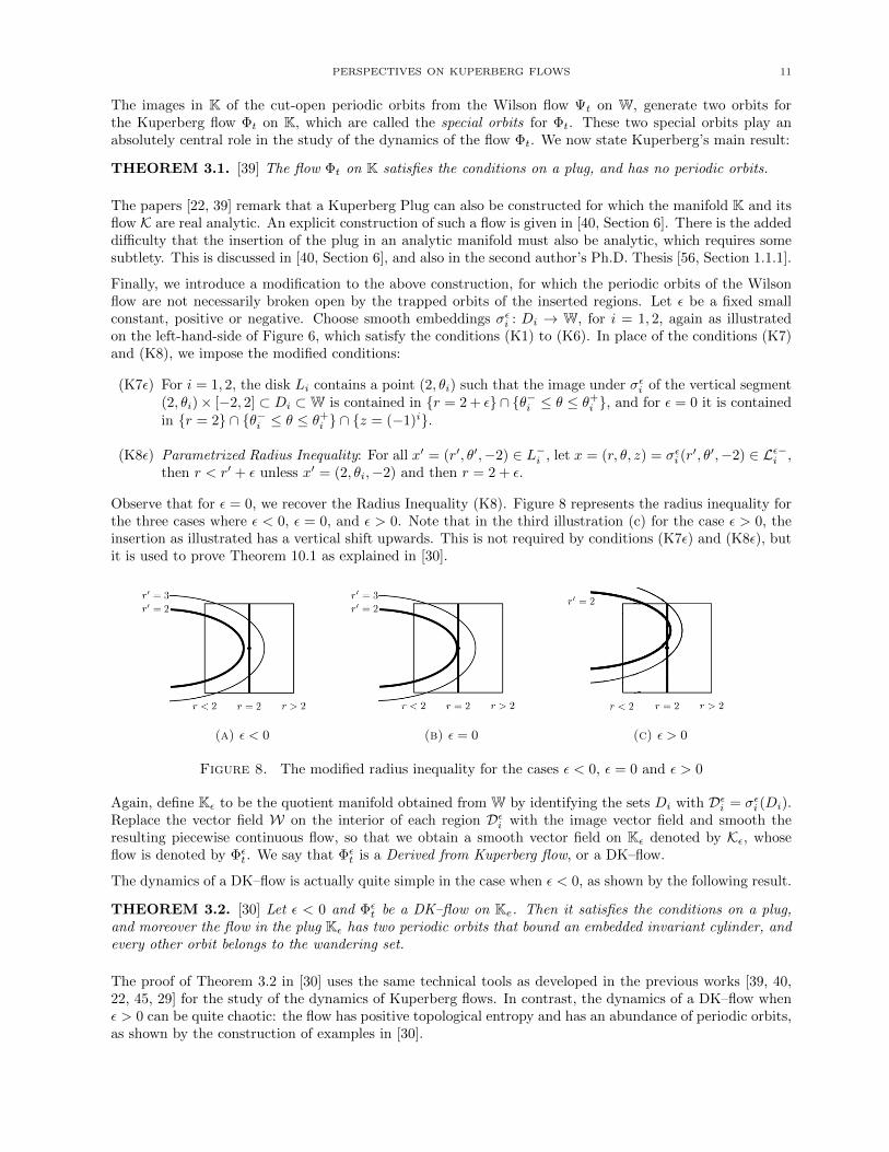
Observe that for ε = 0, we recover the Radius Inequality (K8). Figure 8 represents the radius inequality forthe three cases where ε < 0, ε = 0, and ε > 0. Note that in the third illustration (c) for the case ε > 0, theinsertion as illustrated has a vertical shift upwards. This is not required by conditions (K7ε) and (K8ε), butit is used to prove Theorem 10.1 as explained in [30].

(a) ε < 0 (b) ε = 0 (c) ε > 0

Figure 8. The modified radius inequality for the cases ε < 0, ε = 0 and ε > 0

Again, define Kε to be the quotient manifold obtained from W by identifying the sets Di with Dεi = σεi (Di).Replace the vector field W on the interior of each region Dεi with the image vector field and smooth theresulting piecewise continuous flow, so that we obtain a smooth vector field on Kε denoted by Kε, whoseflow is denoted by Φεt. We say that Φεt is a Derived from Kuperberg flow, or a DK–flow.

The dynamics of a DK–flow is actually quite simple in the case when ε < 0, as shown by the following result.

THEOREM 3.2. [30] Let ε < 0 and Φεt be a DK–flow on Ke. Then it satisfies the conditions on a plug,and moreover the flow in the plug Kε has two periodic orbits that bound an embedded invariant cylinder, andevery other orbit belongs to the wandering set.

The proof of Theorem 3.2 in [30] uses the same technical tools as developed in the previous works [39, 40,22, 45, 29] for the study of the dynamics of Kuperberg flows. In contrast, the dynamics of a DK–flow whenε > 0 can be quite chaotic: the flow has positive topological entropy and has an abundance of periodic orbits,as shown by the construction of examples in [30].


4. Generic hypotheses

The construction of aperiodic Kuperberg flows involve multiple choices, which do not change whether theresulting flows are aperiodic, but do impact other dynamical properties of these flows. In this section,we discuss these choices in more detail, and introduce the generic assumptions that were imposed in theworks [29, 30]. The implications of these choices will be discussed in subsequent sections. We first discussthe choices made in constructing the modified Wilson plug, then consider the even wider range of choicesinvolved with the construction of the insertion maps. We discuss first the case for the traditional Kuperbergflows, and afterwards discuss the variations of the construction.

Recall that the modified Wilson vector field on W is given in (3) by

W = g(r, θ, z)∂

∂z+ f(r, θ, z)

∂

∂θ

where the function g(r, θ, z) = g(r, z) is the suspension of the function g : R→ [0, g0] which is non-negative,vanishing only at the points (2,±1), and symmetric about the line z = 0. The function f(r, θ, z) = f(r, z)is assumed to satisfy the conditions (W1) to (W6), though conditions (W5) and (W6) are imposed to simplifycalculations, and do not impact the aperiodic conclusion for the Kuperberg flows.

Figure 2 illustrates the dynamics of the flow of W restricted to the cylinders r = cst in W, for variousvalues of the radius. It is clear from these pictures that the “interesting” part of the dynamics of this flowoccurs on the cylinders with radius near to 2, and near the periodic orbits Oi for i = 1, 2.

The points (2,±1) ∈ R are the local minima for the function g, and thus its matrix of first derivatives mustalso vanish at these points, and the Hessian matrix of second derivatives must be positive semi-definite. Thegeneric property for such a function is that the Hessian matrix for g at these points is positive definite. Inthe works [29, 30], a more precise version of this was formulated:

HYPOTHESIS 4.1. The function g satisfies the following conditions:

(7) g(r, z) = g0 for (r − 2)2 + (|z| − 1)2 ≥ ε20where 0 < ε0 < 1/4 is sufficiently small. Moreover, we require that the Hessian matrices of second partialderivatives for g at the vanishing points (2,±1) are positive definite. In addition, we require that g(r, z) is

monotone increasing as a function of the distance√

(r − 2)2 + (|z| − 1)2 from the points (2,±1).

The conclusions of Proposition 2.1 do not require Hypothesis 4.1, and so Theorem 3.1 does not require it.On the other hand, many of the results in [29, 30] do require this generic hypothesis for their proofs, as itallows making estimates on the “speed of ascent” for the orbits of the Wilson flow near the periodic orbits.

Hypothesis 4.1 implies a local quadratic estimate on the function g near the points (2,±1) which is given asestimate (94) in [29]. We formulate a more general version of this local estimate for g.

HYPOTHESIS 4.2. Let n ≥ 2 be an even integer. We say that the vector field W on W vanishes withorder n if there exists constants λ2 ≥ λ1 > 0 and ε0 > 0 such that

(8) λ1 ((r − 2)n + (|z| − 1)n) ≤ g(r, z) ≤ λ2 ((r − 2)n + (|z| − 1)n) for ((r − 2)n + (|z| − 1)n) ≤ εn+20 .

Hypothesis 4.1 implies that Hypothesis 4.2 holds for n = 2. This yields an estimate on the speed which theorbits of W in W for points with z 6= ±1 approach the periodic orbits Oi in forward or backward time, asdiscussed in detail in [29, Chapter 17]. When n > 2, this speed of approach becomes slower and slower as ngets larger. We can also allow for the case where g has all partial derivatives vanishing at the points (2,±1),in which case we say that the function g vanishes to infinite order at the critical points, and we say thatthe resulting vector field W on W is infinitely flat at Oi for i = 1, 2. In that case, the speed of approach oforbits of W in W become arbitrarily slow towards the periodic orbits.

The choices for the embeddings σi : Di → W, for i = 1, 2, as illustrated on the left-hand-side of Figure 6,are more wide-ranging, and have a fundamental influence on the dynamics of the resulting Kuperberg flowson the quotient space K. We first impose a “normal form” condition on the insertions, which does not have


significant impact on the dynamics, but allows a more straightforward formulation of the other propertiesof the insertion maps.

Let (r, θ, z) = σi(x′) ∈ Di for i = 1, 2, where x′ = (r′, θ′, z′) ∈ Di is a point in the domain of σi. Let

πz(r, θ, z) = (r, θ,−2) denote the projection of W along the z-coordinate. We assume that σi restricted tothe bottom face, σi : L

−i → W, has image transverse to the vertical fibers of πz. This normal form can be

achieved by an isotopy of a given embedding along the flow lines of the vector field W, so does not changethe orbit structure of the resulting vector field on the plug K.

The above transversality assumption implies that πz σi : L−i →W is a diffeomorphism into the face ∂−h W,

with image denoted by Di ⊂ ∂−h W. Then let ϑi = (πz σi)−1 : Di → L−i denote the inverse map, so we have:

(9) ϑi(r, θ,−2) = (r(ϑi(r, θ,−2)), θ(ϑi(r, θ,−2)),−2) = (Ri,r(θ),Θi,r(θ),−2) .

We can then formalize in terms of the maps ϑi the assumptions on the insertion maps σi that are intuitivelyimplicit in Figure 6, and will be assumed for all insertion maps considered.

HYPOTHESIS 4.3 (Strong Radius Inequality). For i = 1, 2, assume that:

(1) σi : L−i →W is transverse to the fibers of πz;

(2) r = r(σi(r′, θ′, z′)) < r′, except for (2, θi, z

′) and then z(σi(2, θi, z′)) = (−1)i;

(3) Θi,r(θ) = θ(ϑi(r, θ,−2)) is an increasing function of θ for each fixed r;

(4) Ri,r(θ) = r(ϑi(r, θ,−2)) has non-vanishing derivative for r = 2, except for the case of θi defined by

ϑi(2, θi,−2) = (2, θi,−2);(5) For r sufficiently close to 2, we require that the θ derivative of Ri,r(θ) vanish at a unique point

denoted by θ(i, r).

Consequently, each surface L−i is transverse to the coordinate vector fields ∂/∂θ and ∂/∂z on W.

The illustration of the image of the curves r′ = 2 and r′ = 3 on the right-hand-side of Figure 6 suggests thatthese curves have “parabolic shape”. We formulate this notion more precisely using the function ϑi(r, θ,−2)defined by (9), and introduce the more general hypotheses they may satisfy. Recall that ε0 > 0 was introducedin Hypothesis 4.1.

HYPOTHESIS 4.4. Let n ≥ 2 be an even integer. For i = 1, 2, 2 ≤ r0 ≤ 2 + ε0 and θi − ε0 ≤ θ ≤ θi + ε0,assume that

(10)d

dθΘi,r0(θ) > 0 ,

dn

dθnRi,r0(θ) > 0 ,

d

dθRi,r0(θi) = 0 ,

d`

dθ`Ri,r0(θi) = 0 for 1 ≤ ` < n .

where θi satisfies ϑi(2, θi,−2) = (2, θi,−2). Thus for 2 ≤ r0 ≤ 2+ε0, the graph of Ri,r0(θ) is convex upwards

with vertex at θ = θi.

In the case where n = 2, Hypothesis 4.4 implies that all of the level curves r′ = c, for 2 ≤ c ≤ 2 + ε0, haveparabolic shape, as the illustration in Figure 6 suggests. On the other hand, for n > 2 the level curves r′ = chave higher order contact with the vertical lines of constant radius in Figure 6, and in this case, many of thedynamical properties of the resulting flow Φt on K are not well-understood.

We can now define what is called a generic Kuperberg flow in the work [29].

DEFINITION 4.5. A Kuperberg flow Φt is generic if the Wilson flow W used in the construction of thevector field K satisfies Hypothesis 4.1, and the insertion maps σi for i = 1, 2 used in the construction ofK satisfies Hypotheses 4.3, and Hypotheses 4.4 for n = 2. That is, the singularities for the vanishing ofthe vertical component g · ∂/∂z of the vector field W are of quadratic type, and the insertion maps used toconstruct K yield quadratic radius functions near the special points.

Recall that the insertion maps for a Derived from Kuperberg flow as introduced in Section 3 are denoted byσεi : Di → W, for i = 1, 2. It is assumed that these maps satisfy the modified conditions (K7ε) and (K8ε).The illustrations of the radius inequality in Figure 8 again suggest that the images of the curves r′ = c areof “quadratic type”, though the vertex of the image curves need no longer be at a special point. We again


assume the insertion maps σεi : L−i → W are transverse to the fibers of the projection map πz : W → ∂−h Walong the z′-coordinate. Then we can define the inverse map ϑεi = (πz σεi )−1 : Di → L−i and express theinverse map x′ = ϑεi(x) in polar coordinates as:

(11) x′ = (r′, θ′,−2) = ϑεi(r, θ,−2) = (r(ϑεi(r, θ,−2)), θ(ϑεi(r, θ,−2)),−2) = (Rεi,r(θ),Θεi,r(θ),−2) .

Then the level curves r′ = c pictured in Figure 8 are given by the maps θ′ 7→ πz(σεi (c, θ

′,−2)) ∈ ∂−h W.

We note a straightforward consequence of the Parametrized Radius Inequality (K8ε). Recall that θi is theradian coordinate specified in (K8ε) such that for x′ = (2, θi,−2) ∈ L−i we have r(σεi (2, θi,−2)) = 2 + ε.

LEMMA 4.6. [30, Lemma 6.1] For ε > 0 there exists 2 + ε < rε < 3 such that r(σεi (rε, θi,−2)) = rε.

We then add an additional assumption on the insertion maps σεi for i = 1, 2 which specifies the qualitativebehavior of the radius function for r ≥ rε.

HYPOTHESIS 4.7. If rε is the smallest 2 + ε < rε < 3 such that r(σεi (rε, θi,−2)) = rε. Assume thatr(σεi (r, θi,−2)) < r for r > rε.

The conclusion of Hypothesis 4.7 is implied by the Radius Inequality for the case ε = 0, but does not followfrom the condition (K8ε) when ε > 0. It is imposed to eliminate some of the possible pathologies in thebehavior of the orbits of the DK–flows.

We can now formulate the analog for DK–flows of the Hypothesis 4.3, which imposes uniform conditions onthe derivatives of the maps ϑεi . Recall that 0 < ε0 < 1/4 was specified in Hypothesis 4.1, and we assumethat 0 < ε < ε0.

HYPOTHESIS 4.8 (Strong Radius Inequality). For i = 1, 2, assume that:

(1) σεi : L−i →W is transverse to the fibers of πz;(2) r = r(σεi (r

′, θ′, z)) < r + ε, except for x′ = (2, θi, z) and then r = 2 + ε;(3) Θε

i,r(θ) is an increasing function of θ for each fixed r;(4) For 2− ε0 ≤ r ≤ 2 + ε0 and i = 1, 2, assume that Rεi,r(θ) has non-vanishing derivative, except when

θ = θi as defined by ϑεi(2 + ε, θi,−2) = (2, θi,−2);(5) For r sufficiently close to 2 + ε, we require that the θ derivative of Rεi,r(θ) vanishes at a unique point

denoted by θ(i, r).

Note that Hypotheses 4.7 and 4.8 combined imply that rε is the unique value of 2 + ε < rε < 3 for whichr(σεi (rε, θi,−2)) = rε. We can then formulate the analog of Hypothesis 4.4.

HYPOTHESIS 4.9. Let n ≥ 2 be an even integer. For 2 − ε0 ≤ r0 ≤ 2 + ε0 and θi − ε0 ≤ θ ≤ θi + ε0,assume that

(12)d

dθΘεi,r0(θ) > 0 ,

dn

dθnRεi,r0(θ) > 0 ,

d

dθRεi,r0(θi) = 0 ,

d`

dθ`Rεi,r0(θi) = 0 for 1 ≤ ` < n .

where θi satisfies ϑεi(2, θi,−2) = (2, θi,−2). Thus for 2 − ε0 ≤ r0 ≤ 2 + ε0, the graph of Rεi,r0(θ) is convex

upwards with vertex at θ = θi.

Finally, we have the definition of the generic DK–flows studied in [30].

DEFINITION 4.10. A DK–flow Φεt is generic if the Wilson flow W used in the construction of the vectorfield Kε satisfies Hypothesis 4.1, and the insertion maps σεi for i = 1, 2 used in the construction of Kε satisfiesHypotheses 4.8, and Hypotheses 4.9 for n = 2.


5. Wandering and minimal sets

We next discuss some of the basic topological dynamical properties of the Kuperberg flows. Our maininterest is in the asymptotic behavior of their orbits, especially the non-wandering and wandering sets forthe flow. There is an additional subtlety in these considerations, in that many orbits for the flow in a plugmay escape from the plug, while other orbits are trapped in either the forward or backward directions, orpossibly both. We also recall the results about the uniqueness of the minimal set. First we recall some ofthe basic concepts for the flow in a plug.

Recall that Di = σi(Di) for i = 1, 2 are solid 3-disks embedded in W. Introduce the sets:

(13) W′ ≡ W− D1 ∪ D2 , W ≡ W− D1 ∪ D2 .

The compact space W ⊂W is the result of “drilling out” the interiors of D1 and D2.

Let τ : W → K denote the quotient map. Note that the restriction τ ′ : W′ → K is injective and onto, whilefor i = 1, 2, the map τ identifies a point x ∈ Di with its image σi(x) ∈ Di. Let (τ ′)−1 : K→W′ denote theinverse map, which followed by the inclusion W′ ⊂ W, yields the (discontinuous) map τ−1 : K → W, wherei = 1, 2, we have:

(14) τ−1(τ(x)) = x for x ∈ Di , and σi(τ−1(τ(x))) = x for x ∈ Di .

Consider the embedded disks L±i ⊂ W defined by (5), which appear as the faces of the insertions in W.Their images in the quotient manifold K are denoted by:

(15) E1 = τ(L−1 ) , S1 = τ(L+1 ) , E2 = τ(L−2 ) , S2 = τ(L+

2 ) .

Note that τ−1(Ei) = L−i , while τ−1(Si) = L+i .

The transition points of an orbit of Φt are those points where the orbit intersects one of the sets Ei or Sifor i = 1, 2, or is contained in a boundary component ∂−h K or ∂+h K. The transition points are classified aseither primary or secondary, where x ∈ K is:

• a primary entry point if x ∈ ∂−h K;

• a primary exit point if x ∈ ∂+h K;• a secondary entry point if x ∈ E1 ∪ E2;• a secondary exit point x ∈ S1 ∪ S2.

If a Φt-orbit of a point x ∈ K contains no transition points, then the restriction τ−1(Φt(x)) is a continuousfunction of t, and is contained in the Ψt-orbit of x′ = τ−1(x) ∈W.

Recall that r : W → [1, 3] is the radius coordinate on W. Define the (discontinuous) radius coordinater : K → [1, 3], where for x ∈ K set r(x) = r(τ−1(x)). Then for x ∈ K set ρx(t) ≡ r(Φt(x)), which is theradius coordinate function along the K-orbit of x. Note that if Φt0(x) is not an entry/exit point, then thefunction ρx(t) is locally constant at t0. On the other hand, if t0 is a point of discontinuity for Φt(x), thenx0 = Φt0(x) must be a secondary entry or exit point.

These properties of the radius function along orbits of the flow Φt gives a strategy for the study of thedynamics of the flow, and provides the key technique in [39] used to prove that the flow is aperiodic. A keyidea is to index the points along the orbit of a point x ∈ K by the intersections with the sets E1 ∪ E2, forwhich the index increases by +1, or their intersection with the sets S1 ∪ S2, for which the index decreasesby −1. This yields the integer-valued level function nx(t) which has nx(0) = 0.

Recall that Oi for i = 1, 2 denotes the periodic orbits for the Wilson flow on W, so that each intersectionOi ∩W′ consists of an open connected arc with endpoints L±i ∩ Oi. The special entry/exit points for theflow Φt are the images, for i = 1, 2,

(16) p−i = τ(Oi ∩ L−i ) ∈ Ei , p+i = τ(Oi ∩ L+i ) ∈ Si .

Note that by definitions and the Radius Inequality, we have r(p±i ) = 2 for i = 1, 2.


We now recall the results for the minimal set of aperiodic Kuperberg flows based on the combined resultsfrom the works [22, 39, 40, 45]. It was observed by Kuperberg in [39] that for x ∈ K with r(x) = 2, theneither its forward orbit Φt(x) | t ≥ 0 contains a special point in its closure, or this is true for the backwardorbit Φt(x) | t ≤ 0, or both conditions hold. Also, for x ∈ K if the radius function ρx(t) ≥ c for somec > 2, then the orbit of x escapes in finite time in both forward and backward directions. It follows fromthis that for x ∈ K with r(x) > 2 and whose orbit is infinite in either forward or backward directions, thenits orbit closure must contain at least one of the special orbits.

It was observed in Matsumoto [45] that there is an open set of primary entry points with radius less than2 whose forward orbits are non-recurrent and yet accumulate on the special orbits. Ghys showed in [22,Theoreme, page 301] that if x ∈ K does not escape from K in a finite time, either forward or backward, thenthe orbit of the point accumulates on the special orbits. These results combined imply that a Kuperbergflow has a unique minimal set contained in the interior of K.

We state these results more succinctly as follows. Define the following orbit closures in K:

(17) Σ1 ≡ Φt(p−1 ) | −∞ < t <∞ , Σ2 ≡ Φt(p−2 ) | −∞ < t <∞ .THEOREM 5.1. [29, Theorem 8.2] For the closed sets Σi for i = 1, 2 we have:

(1) Σi is Φt-invariant;(2) r(x) ≥ 2 for all x ∈ Σi;(3) Σ1 = Σ2 and we set Σ = Σ1 = Σ2;(4) Let Z ⊂ K be a closed invariant set for Φt contained in the interior of K, then Σ ⊂ Z;(5) Σ is the unique minimal set for Φt.

The orbits of the Kuperberg flow are divided into those which are finite, forward or backward trapped, ortrapped in both directions and so infinite. A point x ∈ K is forward wandering if there exists an open setx ∈ U ⊂ K and TU > 0 so that for all t ≥ TU we have Φt(U) ∩ U = ∅. Similarly, x is backward wandering ifthere exists an open set x ∈ U ⊂ K and TU < 0 so that for all t ≤ TU we have Φt(U) ∩ U = ∅. A point xwith infinite orbit is wandering if it is forward and backward wandering. Define the following subsets of K:

W0 ≡ x ∈ K | x orbit is finiteW+ ≡ x ∈ K | x orbit is forward wanderingW− ≡ x ∈ K | x orbit is backward wanderingW∞ ≡ x ∈ K | x is forward and backward wandering

Note that x ∈ W0 if and only if the orbit of x escapes through ∂+h K in forward time, and escapes though

∂−h K in backward time. Define

(18) W = W0 ∪W+ ∪W− ∪W∞ ; Ω = K−W.

The set Ω is called the non-wandering set for Φt, is closed and Φt-invariant. A point x with forwardtrapped orbit is characterized by the property: x ∈ Ω if for all ε > 0 and T > 0, there exists y and t > Tsuch that dK(x, y) < ε and dK(x,Φt(y)) < ε, where dK is a distance function on K. There are obviouscorresponding statements for points which are backward trapped or infinite. Here are some of the propertiesof the wandering and non-wandering sets for Kuperberg flows. The proofs can be found in [29, Chapter 8].

LEMMA 5.2. If x ∈ K is a primary entry or exit point, then x ∈W+ or W−.

LEMMA 5.3. For each x ∈ Ω, the Φt-orbit of x is infinite.

PROPOSITION 5.4. Σ ⊂ Ω ⊂ x ∈ K | r(x) ≥ 2.

Finally, let us recall a result of Matsumoto:

THEOREM 5.5. [45, Theorem 7.1(b)] The sets W± contain interior points.

This implies the following important consequence:

COROLLARY 5.6. The flow Φt cannot preserve any smooth invariant measure on K which assigns positivemass to any open neighborhood of a special point.


6. Zippered laminations

We next introduce the Φt-invariant embedded surface M0 and its closure M, and discuss the relation betweenthe minimal set Σ and the space M. The existence of this compact connected subset M, which is invariantfor the Kuperberg flow Φt, is a remarkable consequence of the construction of Φt, and is the key to a deeperunderstanding of the properties of the minimal set Σ of Φt. We then give an overview of the structure theoryfor M0 which plays a fundamental role in analyzing the dynamical properties of Kuperberg flows.

Recall that the Reeb cylinder R ⊂W is bounded by the two periodic orbits O1 and O2 for the Wilson flowΨt on W. The cylinder R is itself invariant under this flow, and for a point x ∈W with r(x) close to 2, theΨt-orbit of x has increasingly long orbit segments which shadow the periodic orbits.

Introduce the notched Reeb cylinder, R′ = R ∩W′, which has two closed “notches” removed from R whereit intersects the closed insertions Di ⊂ W for i = 1, 2. Figure 9 illustrates the cylinder R′ inside W. Theboundary segments γ′ and λ′ labeled in Figure 9 satisfy γ′ ⊂ L−1 and λ′ ⊂ L−2 , while the boundary segments

γ′ and λ′

labeled in Figure 9 satisfy γ′ ⊂ L+1 and λ

′ ⊂ L+2 . A basic observation is that these curves are each

transverse to the restriction of the Wilson flow to the cylinder R.

Figure 9. The notched cylinder R′ embedded in W

The map τ : R′ → K is an embedding, so the Φt-flow of τ(R′) ⊂ K is an embedded surface,

(19) M0 ≡ Φt(τ(R′)) | −∞ < t <∞ .

The special orbits in K contain the intersection τ(Oi∩W′) for i = 1, 2, hence the “boundary” of M0 consistsof the two special orbits in K obtained by the Φt-flows of the arcs τ(Oi ∩W′), so that M0 is an “infinitebordism” between the two special orbits of the flow Φt. Thus, the closure M = M0 is a flow invariant,compact connected subset of K, which contains the closure of the special orbits, hence by Theorem 5.1, theminimal set Σ ⊂M.

A fundamental problem is to give a description of the topology and geometry of the space M. The questionof when Σ = M is treated in Section 7, while in this section we concentrate on the properties of M.

The key to understanding the structure of the space M is to analyze the structure of M0 and its embeddingin K. This analysis is based on a simple observation, that the images τ(γ′), τ(λ′) ⊂M are curves transverseto the flow Φt and contained in the region x ∈M | r(x) ≥ 2. Moreover, for a point x ∈ τ(γ′) with r(x) > 2,there is a finite tx > 0 such that Φtx(x) ∈ τ(γ′). That is, the flow across the notch in τ(R′) with boundarycurve τ(γ′) closes up by returning to the facing boundary curve τ(γ′), unless r(x) = 2 and then x is the

special point p−1 . A similar remark holds for the notch in R′ with boundary curves λ′, λ′. It follows from the

proof of the above remarks that we can analyze the submanifold M0 using a recursive approach, decomposingthe space into the flows in K of the curves of successive intersections with the entry/exit surfaces Ei and Si.

PROPOSITION 6.1. [29, Proposition 10.1] There is a well-defined level function

(20) n0 : M0 → N = 0, 1, 2, . . . ,


where the preimage n−10 (0) = τ(R′), the preimage n−10 (1) in the union of two infinite notched propellerswhich are asymptotic to τ(R′), and for ` > 1 the preimage n−10 (`) is an infinite union of finite notchedpropellers.

The precise description of propellers, both finite and infinite, is given in [29, Chapters 11, 12], and thedecomposition is made precise there. We give a general sketch of the idea.

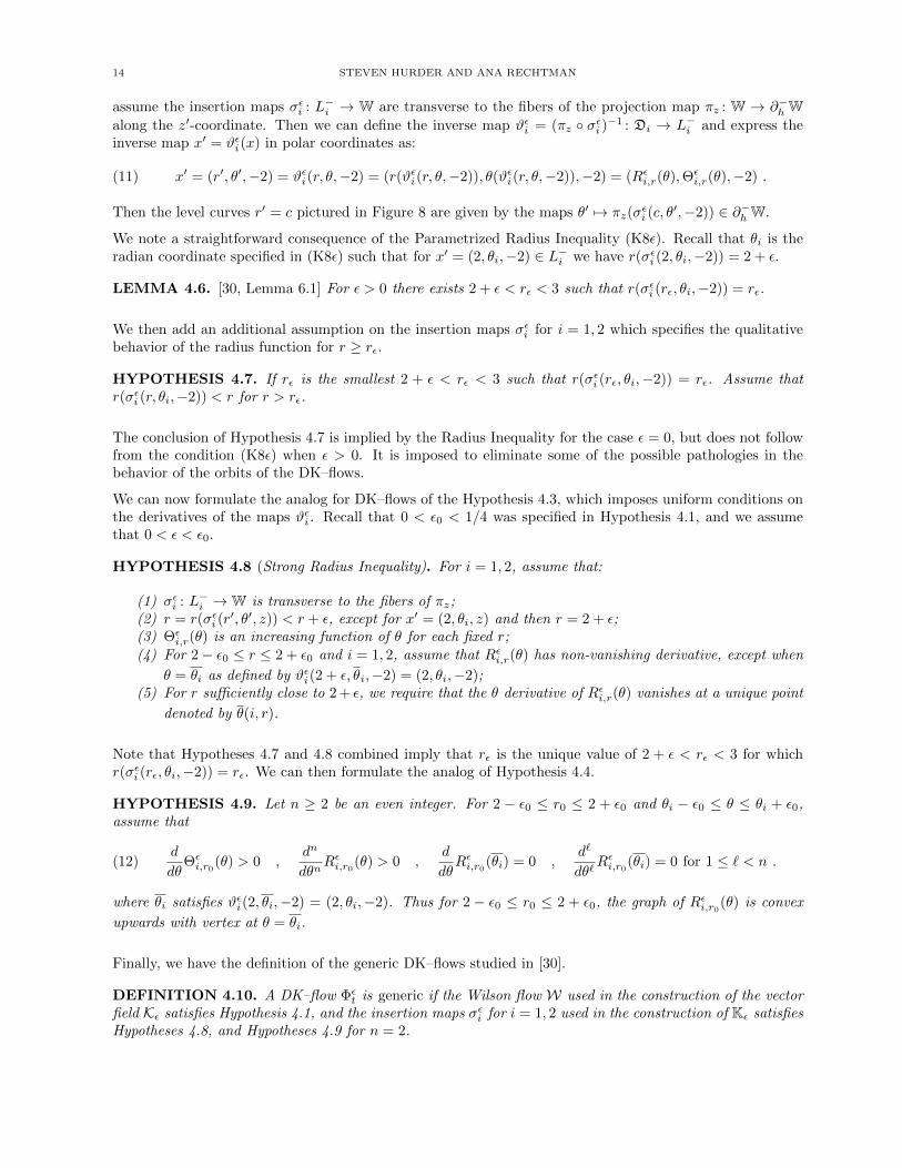
A propeller is an embedded surface in W that results from the Wilson flow Ψt of a curve γ ⊂ ∂−h W in thebottom face of W. Such a surface has the form of a “tongue” wrapping around the core cylinder C. Figure 10illustrates a “typical” finite propeller Pγ as a compact “flattened” propeller on the right, and its embeddingin W on the left. Observe that in this case, for any x ∈ γ, the radius of x is strictly bigger than 2.

Figure 10. Embedded and flattened finite propeller

An infinite propeller is the result of flowing a curve γ which has endpoint on the cylinder r = 2, hence theflow of the compact curve is not closed, as its boundary curve is the orbit of an entry point with radius 2,hence limits on the Reeb cylinder R. The embedding of an infinite propeller is highly dependent on theshape of the curve γ near the cylinder C, and on the dynamics of the Wilson flow near its periodic orbits.

Figure 11 gives a model for M0, though the distances along propellers are not to scale, and there is a hiddensimplification in that there may be “bubbles” in the surfaces which are suppressed in the illustration. Abubble is a compact surface with boundary attached to the interior regions of a propeller along its boundary,and are analyzed in Chapters 15 and 18 of [29]. Also, all the propellers represented in Figure 11 have roughlythe same width when embedded in K, which is the width of the Reeb cylinder.

We make some further comments on the properties of M0 as illustrated in Figure 11. The upper horizontalband the figure represents the notched Reeb cylinder. The flow of the special point p−1 is the curve along thebottom edge of the image τ(R′). When the flow crosses the curve τ(γ) = τ(R′) ∩ E1, it turns to the rightand enters the infinite propeller at level 1, and follows the left edge of this vertical strip downward, alongthe Wilson flow of a point with r = 2 until it intersects the secondary entry surface E1 again. It then turnsto the right in the flow direction, and enters a finite propeller at level 2. In the case pictured, it then flowsupward until it crosses the annulus A = z = 0 ⊂W, which corresponds to the tip of the propeller. It thenreverses direction and flows until it crosses the secondary exit surface S1, and resumes flowing downwardalong the infinite level 1 propeller. However, as this is following a Wilson orbit, the z-values of this part ofthe orbit are increasing towards −1.

This procedure continues repeatedly, though as the curve moves further down the level 1 propeller, thez-values get closer to −1, and hence the flow in the side level 2 propellers intersects the secondary entryregion E1 increasingly often, before flowing through the tip of the corresponding level 2 propeller, andreversing its march through either a secondary exit surface Si or another secondary entry face Ei. Thisprocess can be viewed as a geometric model for the recursive description of the flow dynamics as describedusing programming language in [40, Section 5]. A key point is that the lengths of the side branches, whilefinite, increase in length and branching complexity as the orbit moves downwards along the vertical level 1propeller. A similar scenario plays out when following the upper infinite propeller, whose initial segment isall that is illustrated in Figure 11.


Figure 11. Flattened part of M0

The two infinite propellers which constitute n−10 (1) are well-understood, but the finite propellers whichconstitute the sets n−10 (`) for ` > 1 (pictured as the side branching surfaces in Figure 11) may defy asystematic description without imposing some form of generic hypotheses on the construction of the flow.On the other hand, for a generic Kuperberg flow as in Definition 4.5, the work [29] gives a reasonablycomplete description of the components of the level decomposition of M0. These results are used to show:

THEOREM 6.2. [29, Theorem 19.1] If Φt is a generic Kuperberg flow on K, then the closure M in W ofM0 is a zippered lamination.

The definition of a zippered lamination is technical, and given in [29, Definition 19.3]. The notion can besummarized by the conditions that M is a union of 2-dimensional submanifolds of M, and admits a finitecover by special foliation charts which are maps of subsets of M to a measurable product of a disk withboundary in R2 with a Cantor set. In particular, this covering property enables the construction of thetransverse holonomy maps along the leaves of the lamination M. The structure of the submanifold M0 iskey to understanding the entropy invariants of the flow, and also conjecturally the Hausdorff dimensions ofits closed invariant sets, as will be discussed further in Section 8.

7. Denjoy Theory for laminations

The fundamental problem in the study of the dynamics of a Kuperberg flow is to understand the ergodicand topological structure of its unique minimal set Σ. Surprisingly, the ergodic properties of a flow Φt is theleast well-understood aspect of its dynamics. Since there is a unique minimal set, here is the basic question:

PROBLEM 7.1. Show that the restriction of a Kuperberg flow to its minimal set is uniquely ergodic. Ifnot, characterize the invariant probability measures for the flow.

We have that Φt is a zero entropy flow on a compact space of dimension at most two, so the problem bearssome resemblance to the problem of showing that the horocycle flow for a 2-dimensional Riemann surfaceof negative curvature is uniquely ergodic, which was proven by Furstenberg [20]. However, the dynamics ofthe flow Φt seems to be much more irregular than for a horocycle flow, as the orbits of Φt cluster around thedeleted Reeb cylinder R′ for long orbit segments, before wandering out far away from R′ in the plug and


then returning. In this sense, the problem may bear more resemblance to the result of Dani and Smillie [13]that the horocycle flow is uniquely ergodic for a Fuchsian group. In any case, the question of whether theKuperberg flows are uniquely ergodic is very basic.

The remainder of this section will consider questions about the topological dynamics of the flow Φt restrictedto the invariant space M. In Section 9 of the paper [40], the authors assert:

Although most aperiodic self-inserted Wilson-type plugs have 2-dimensional minimal sets, acarefully chosen self-intersection may result in a 1-dimensional minimal set.

Since we always have Σ ⊂M, the above remark highlights the importance of the following problem:

PROBLEM 7.2. Give conditions on a Kuperberg flow which imply that Σ = M.

The equality Σ = M is a remarkable conclusion, as the flow of the special orbits p±i ∈ K are dense in Σ andconstitute the boundary of the submanifold M0, so the equality Σ = M implies that the boundaries of apath connected component of M are dense in the space itself! This property seems highly improbable.

The result [22, Theoreme, page 302] states that there exist Kuperberg flows for which Σ = M, and hencethe minimal set Σ is 2-dimensional. The result [40, Theorem 17] gives an explicit analytic flow for whichΣ = M. The idea behind these examples is based on the observation that the orbit Φt(p−1 ) | −∞ < t <∞of a special point p−1 contains the boundary of all the level 2 propellers represented in Figure 11, thus itcontains the tips of these propellers. As the level 2 propellers get longer, the tips have smaller radius thattends to 2. The points corresponding to the tips are contained in the annulus τ(A) = τ(z = 0), and thusaccumulate on the Reeb cylinder τ(R′), and hence on all of M.

The proof of the following result was inspired by the proof of [40, Theorem 17], and uses these ideas to show:

THEOREM 7.3. [29, Theorem 17.1] Let Φt be a generic Kuperberg flow on K, then Σ = M.

The proof of Theorem 7.3 uses the generic hypotheses on both the Wilson flow and the insertion maps, toobtain estimates on the density of the orbit Φt(p−1 ) | −∞ < t <∞ near to τ(R′). While the calculationsin [29] use the quadratic assumptions on the maps, it seems reasonable to expect that the required estimatescan be achieved for more general cases.

PROBLEM 7.4. Let Φt be a Kuperberg flow on K which satisfies Hypothesis 4.2 for some even n ≥ 2,Hypothesis 4.4 for some possibly different value of n ≥ 2, and otherwise satisfies the generic hypotheses.Show that Σ = M.

The hypotheses of Problem 7.4 are essentially satisfied for a real analytic Kuperberg flow, so as a variationon Problem 7.4, we ask whether all real-analytic flows have 2-dimensional minimal sets:

PROBLEM 7.5. Show that Σ = M if Φt is a real analytic Kuperberg flow on K.

We mention another problem concerning real analytic Kuperberg flows.

PROBLEM 7.6. Find dynamical properties of Kuperberg flows which distinguish the real analytic flowsfrom the smooth (possibly non-generic) flows.

Next, consider the case where the inclusion Σ ⊂ M of invariant sets is proper. Then Σ is a closed 1-dimensional invariant set in a lamination, which must have some remarkable properties as a subspace of M.It is not known if such examples can exist for C1-flows, for example, so we propose:

PROBLEM 7.7. Construct a C1 Kuperberg flow for which the minimal set Σ is 1-dimensional.

One approach might be to perturb a smooth Kuperberg flow in the C1-topology to obtain a Denjoy-typeminimal set contained in the lamination M, which would be a “wild” version of a Schweitzer plug.

The notion of piecewise-linear (PL)-flows in a plug was developed in Section 8 of [40], and these flowsyield a class of dynamical systems on a plug which are distinct from the class of smooth flows. The proof of


Theorem 19 of [40] shows that there are PL-flows on plugs with 1-dimensional minimal sets, though it shouldbe noted that the examples these authors give introduces a modification of the standard construction of theKuperberg plug as given in Section 3. They also describe an example of a PL-flow for which the minimalset is 2-dimensional. These results suggest that the following project should be very interesting:

PROBLEM 7.8. Study the dynamical properties of PL-flows in a Kuperberg plug. Find conditions on theconstructions of such flows which ensure that the minimal set Σ is 1-dimensional.

A good place to start would be to elaborate on the methods introduced in Sections 8 and 9 of [40], andinvestigate the dynamics of the resulting PL-flows.

Finally, the study of the relationship between Σ and M suggests considering a more general problem, whetherthere exists a type of “Denjoy Theorem” for 2-dimensional laminations, or matchbox manifolds in theterminology of [7].

PROBLEM 7.9. Let L be a compact connected 2-dimensional lamination, possibly with boundary, and letX be a smooth vector field tangent to the leaves of L. If the boundaries of the leaves of L are non-empty, wealso assume that X is tangent to the boundary. Suppose that L is a minimal lamination, and the flow of Xhas no periodic orbits, then show that every orbit is dense.

The question is whether the equality Σ = M for Kuperberg flows might follow from a more general “DenjoyPrinciple” which is independent of the embedding of the space M ⊂ K. For example, can the proof of thetraditional Denjoy Theorem for C2-flows on the 2-torus T2 be adapted to work for laminations? If so, whatare the minimal hypotheses required to obtain such a result?

8. Growth, slow entropy, and Hausdorff dimension

We next consider invariants of Kuperberg flows derived from the choice of a Riemannian metric on K. Theseinclude the growth rate of area for the embedded surface M0 ⊂ K, the slow entropy of the flow Φt on K, andthe Hausdorff dimensions of the closed invariant sets Σ and M. The authors work [29] gives partial resultson the entropy properties for generic flows, and the work of Ingebretson [35] studies the Hausdorff dimensionof M, but almost nothing is known about these dynamical invariants for the case of non-generic flows.

We first consider the geometric properties of the invariant set M. Recall that M is defined as the closureof the connected infinite surface M0 with boundary, where M0 is defined in (19) as the infinite flow of thenotched Reeb cylinder R′. In general, one approach to studying the dynamics of a smooth flow on a compactmanifold M is to consider the action of the flow on embedded surfaces in M . For example, Yomdim’s proofof the Shub Entropy Conjecture [24, 61, 68] studies the growth rates of the action of the flow on smoothsimplices ∆k ⊂ M , where ∆k is a simplex of dimension 0 < k < dim(M). For a Kuperberg flow, theessential case is for simplices contained in the laminated space M. The study of the geometric properties ofM0 captures all of this information.

Choose a Riemannian metric on K, then the smooth embedded submanifold M0 ⊂ K with boundary inheritsa Riemannian metric. Let dM denote the associated path-distance function on M0. Fix the basepointω0 = (2, π, 0) ∈ τ(R′) and let Bω0(s) = x ∈ M0 | dM(ω0, x) ≤ s be the closed ball of radius s about thebasepoint ω0. Let Area(X) denote the Riemannian area of a Borel subset X ⊂ M0. Then Gr(M0, s) =Area(Bω0

(s)) is called the growth function of M0.

Given functions f1, f2 : [0,∞)→ [0,∞), we say that f1 . f2 if there exists constants A,B,C > 0 such thatfor all s ≥ 0, we have that f2(s) ≤ A · f1(B · s) + C. Say that f1 ∼ f2 if both f1 . f2 and f2 . f1 hold.This defines an equivalence relation on functions, which is used to define their growth type.

The growth function Gr(M0, s) for M0 depends upon the choice of Riemannian metric on K and basepointω0 ∈M0, however the growth type of Gr(M0, s) is independent of these choices.

We say that M0 has exponential growth type if Gr(M0, s) ∼ exp(s). Note that exp(λ s) ∼ exp(s) for anyλ > 0, so there is only one growth class of “exponential type”. We say that M0 has nonexponential growthtype if Gr(M0, s) . exp(s) but exp(s) 6. Gr(M0, s). We also have the subclass of nonexponential growth


type, where M0 has quasi-polynomial growth type if there exists d ≥ 0 such that Gr(M0, s) . sd. The growthtype of a leaf of a foliation or lamination is an entropy-type invariant of its dynamics, as discussed in [28].

For an embedded propeller Pγ ⊂ K the area of the propeller increases as it makes successive revolutionsaround the core cylinder, as illustrated in Figure 10, and this increase is proportional, with uniform boundsabove and below, to the number of revolutions times the area of the Reeb cylinder R. Thus, the growthtype of Gr(M0, s) is a measure of the number of branches and their length in M0 within a given distance sfrom ω0 along the surface. It is thus a measure of the complexity of the recursive procedure which is usedto define the level decomposition of M0. We first state the most general problem concerning M0.

PROBLEM 8.1. How does the growth type of Gr(M0, s) for a Kuperberg flow depend on the geometry ofthe insertion maps, and the germ of the Wilson vector field in a neighborhood of the periodic orbits?

Here is a more precise question about the growth function:

PROBLEM 8.2. Show that the growth type of Gr(M0, s) for a Kuperberg flow is always nonexponential.

This problem was answered in [29] in the case where the flow is generic. Under the additional hypothesis onthe insertion maps σi for i = 1, 2, which is that they have “slow growth”, the following result is proved.

THEOREM 8.3. [29, Theorem 22.1] Let Φt be a generic Kuperberg flow. If the insertion maps σi for i = 1, 2have “slow growth”, then the growth type of M0 is nonexponential, and satisfies exp(

√s) . Gr(M0, s). In

particular, M0 does not have quasi-polynomial growth type.

The definition of “slow growth” for the insertion maps is given in [29, Definition 21.11], and will not berecalled here, as it requires some background preparations.

The previous theorem suggests two questions:

PROBLEM 8.4. Show that the growth type of Gr(M0, s) for a generic Kuperberg flow whose insertionmaps have slow growth is precisely the growth type of the function exp(

√s).

It seems reasonable to expect this problem has a positive answer. It would also be very interesting to knowif the same growth estimate also applies in the case where the flow is real analytic.

PROBLEM 8.5. Let Φt be a Kuperberg flow on K which satisfies Hypothesis 4.2 for some even n ≥ 2,Hypothesis 4.4 for some possibly different value of n ≥ 2, and otherwise satisfies the generic hypotheses.Calculate the growth type for Gr(M0, s).

One motivation for the study of the growth function Gr(M0, s) is its relation to the topological entropyinvariants for the flow Φt. We first discuss the entropy invariants of the flow Φt, then explain how theseproperties are related.

Entropy is defined using a variation of the Bowen formulation of topological entropy [5, 64] for a flow ϕt ona compact metric space (X, dX), with the definition symmetric in the role of the time variable t. For ε > 0,two points p, q ∈ X are said to be (ϕt, T, ε)-separated if

(21) dX(ϕt(p), ϕt(q)) > ε for some − T ≤ t ≤ T .

A set E ⊂ X is (ϕt, T, ε)-separated if all pairs of distinct points in E are (ϕt, T, ε)-separated. Let s(ϕt, T, ε)be the maximal cardinality of a (ϕt, T, ε)-separated set in X. The growth type of the function s(ϕt, T, ε) iscalled the ε-growth type of ϕt, and we can then study the behavior of the growth type as ε→ 0.

The topological entropy of the flow ϕt is then defined by

(22) htop(ϕt) =1

2· limε→0

lim supT→∞

1

Tlog(s(ϕt, T, ε))

.

Moreover, for a compact space X, the entropy htop(ϕt) is independent of the choice of metric dX .

A relative form of the topological entropy for a flow ϕt can be defined for any subset Y ⊂ X, by requiringthat the collection of distinct (ϕt, T, ε)-separated points used in the definition (21) be contained in Y . Therestricted topological entropy htop(ϕt|Y ) is bounded above by htop(ϕt).


For a flow with zero entropy, de Carvalho [9], and Katok and Thouvenot [37], introduced the notion ofslow entropy as a measure of the complexity of the flow. For 0 < α < 1, the slow entropy measures thesubexponential growth of the ε-separated points, and is given by:

DEFINITION 8.6. For a flow ϕt on X, and α > 0, the α-slow entropy of ϕt is given by

(23) hαtop(ϕt) =1

2· limε→0

lim supT→∞

1

Tαlog(s(ϕt, T, ε))

.

In a later work, Dou, Huang and Park introduced in [14] the derived notion of the entropy dimension of adynamical system, using the notion of slow entropy:

DEFINITION 8.7. For a flow ϕt on X, the entropy dimension of ϕt is given by

(24) Dimh(ϕt) = infα>0

hαtop(ϕt)

= 0 .

For a smooth flow on a compact manifold M , we have 0 ≤ Dimh(ϕt) ≤ 1. Observe that Dimh(ϕt) is notrelated to the dimension of the ambient manifold M .

We now return to the consideration of entropy-type invariants for Kuperberg flows. Katok proved in [36,Corollary 4.4] that for a C2-flow ϕt on a compact 3-manifold, its topological entropy htop(ϕt) is boundedabove by the exponent of the rate of growth of its periodic orbits. In particular, Katok’s result can be appliedto an aperiodic flow obtained by inserting a Kuperberg plug, as mentioned in the introduction in Section 1,from which it follows that:

THEOREM 8.8. Let Φt be a Kuperberg flow, then the restricted entropy htop(Φt|M) = 0.

The proof of [36, Corollary 4.4] used the Pesin Theory for C2-flows [1, 54] to obtain a relationship betweentopological entropy of a flow, its Lyapunov exponents, and the existence of invariant horseshoes in thedynamics of the system. The dynamics of a horseshoe system always includes a dense collection of periodicorbits, so if there are no periodic orbits, then the topological entropy must be zero.

The dynamics of generic Kuperberg flows are explicitly analyzed in [29], and a part of this analysis is togive a direct proof that the topological entropy of the flow vanishes. One key aspect of this analysis isthe estimates on the growth function Gr(M0, s) discussed above. A second key aspect is less obvious but

fundamental. Let R0 be the 2-dimensional rectangular section to the flow, and let M0 be the bi-infinite flow

of the full cylinder C by the flow Φt introduced in [29, Chapter 13]. Then the intersection R0 ∩ M0 is aninfinite family of nested closed curves. Moreover, the induced dynamics of the flow on R0 can be viewed asa type of iterated function system with an infinite number of generating maps, where each generating mapmoves one family of nested curves into another family. This is explained in systematic way in the work ofIngebretson [35]. The entropy of the flow restricted to M can then be calculated in terms of this iteratedfunction system, as shown in [32]. Using these ideas in [29], the authors showed:

THEOREM 8.9. [29, Theorem 1.7] Let Φt be a generic Kuperberg flow, then htop(Φt|M) = 0.

We list several problems about the entropy of Kuperberg flows, which can be considered as “work in progress”:

PROBLEM 8.10. Let Φt be a generic Kuperberg flow. Show that Dimh(Φt) = 1/2.

For the case of non-generic Kuperberg flows, we expect the following results to be true:

PROBLEM 8.11. Let Φt be a Kuperberg flow, and suppose that the growth type of M0 is at least that ofthe function nα, for 0 < α < 1. Show that Dimh(Φt) ≥ α.

PROBLEM 8.12. Let Φt be a Kuperberg flow, and suppose that the Wilson flow used in its constructionis infinitely flat near its periodic orbits. Show that Dimh(Φt) = 0.

The entropy invariants defined above can also be considered for the for PL-versions of the Kuperberg con-struction, as in [40, Section 8]. If we allow the Wilson flow to have a discontinuity in its defining functiong along the periodic orbits, then it is possible to construct Wilson flows for which the special points ωi arehyperbolic attracting orbits. In this case, we propose:


PROBLEM 8.13. Let Φt be a PL Kuperberg flow, constructed from a Wilson flow for which the periodicorbits are hyperbolic attracting when restricted to the cylinder C. Show that htop(Φt|M) > 0.

In general, it seems likely that the dynamical and ergodic theory properties of PL-versions of the Kuperbergconstruction will have a much wider range of possibilities, as suggested by the examples in the work [40].

Finally, we mention some natural questions about the Hausdorff dimension properties of Kuperberg flows.

PROBLEM 8.14. Let Φt be a Kuperberg flow. Estimate the Hausdorff dimension dimH(Σ) of its minimalset Σ and the Hausdorff dimension dimH(M) of the invariant set M.

The best (and only) results to date are in the thesis work of Ingebretson [35]. The difficulty with estimatingthe Hausdorff dimensions of the invariant sets associated with a Kuperberg flow, is that the standard methodsof estimating Hausdorff dimensions of Σ and M do not seem to apply. On the other hand, the sets Σ and Mare both dynamically defined by the action of a pseudogroup GK generated by its return map to a section R0

to the flow in the plug. Ingebretson has shown that for a generic flow, the induced dynamics of the return mapon R0 can be viewed as a variant of an iterated function system with an infinite number of generating maps.One can then define extensions of the Bowen-Ruelle-Sinai pressure function for this type of iterated functionsystem, as in Mauldin and Urbanski [46] for example, to obtain estimates on the Hausdorff dimension for aninvariant Cantor set in R0, which yields the above estimate.

For a general Kuperberg flow, it is natural to first consider the problem of estimating the Hausdorff dimensionof the closed invariant lamination M associated to the flow, as it shares many properties with the genericcase, such as the existence of the nested structure for the intersections with a section R0. However, thestructure of the set M ∩ R0 as a generalized iterated function system is no longer well-understood, andother estimates that are required to define the Perron-Frobenius operator for the restricted for to M are notknown. In any case, the following problem seems like a reasonable test case:

PROBLEM 8.15. Let Φt be a real analytic Kuperberg flow. Estimate the Hausdorff dimension dimH(M)of the invariant lamination M.

We conclude with a general question about the case of PL-flows:

PROBLEM 8.16. Given 1 < α < 3, is it possible to construct a PL Kuperberg flow such that HD(Σ) = α?

For a PL-flow, some aspects of the estimations of the pressure function for the set Σ may be much simplerthan for the generic case. On the other hand, the structure of the set Σ is not well understood at all.

More generally, the PL-flows constructed using the standard Kuperberg plug construction, or possibly someclass of its deformations of the DK type, represent a fascinating are of research. On one hand, the PL-nature of the flow implies a type of discreteness, which should simplify calculations. On the other hand, thedeformations of these flows will admit horseshoes, which limit to the aperiodic flow. So one expects a richclass of dynamical systems to result from this construction.

9. Shape theory for the minimal set

Shape theory studies the topological properties of a topological space Z using a form of Cech homotopytheory, and this is the natural framework for the study of topological properties of the minimal set Σ of aKuperberg flow. For example, Krystyna Kuperberg posed the question whether Σ has stable shape? Stableshape is discussed below, and is about the nicest property one can expect for a minimal set that is nota compact submanifold. There are other more delicate shape properties of these spaces to consider. Theknown results about the shape properties of Σ are all for the generic case.

We first give a brief introduction to the notions of shape theory, and introduce stable shape and the movableproperty, then discuss the known results and some problems.

The definition of shape for a topological space Z was introduced by Borsuk [2, 4]. Later developments andresults of shape theory are discussed in the texts [15, 43] and the historical essay [44]. See also the works ofFox [18] and Morita [48].


Recall that a continuum is a compact, connected metrizable space. For example, the subspaces Σ and M ofK are compact and connected, so are continua. We discuss below shape theory for continua.

DEFINITION 9.1. Let Z ⊂ X be a continuum embedded in a metric space X. A shape approximation ofZ is a sequence U = U` | ` = 1, 2, . . . satisfying the conditions:

(1) each U` is an open neighborhood of Z in X which is homotopy equivalent to a compact polyhedron;

(2) U`+1 ⊂ U` for ` ≥ 1, and their closures satisfy⋂`≥1

U ` = Z.

There is a notion of equivalence of shape approximations for continua Z and Z′. In the case where thesespaces are embedded in a manifold, the notion of equivalence is discussed in [29, Chapter 23]. Otherwise,any of the sources cited above give the more general definitions of equivalence of shape approximations.

DEFINITION 9.2. Let Z ⊂ X be a compact subset of a connected manifold X. Then the shape of Z isdefined to be the equivalence class of a shape approximation of Z as above.

It is a basic fact of shape theory that two homotopy equivalent continua have the same shape. Completedetails and alternate approaches to defining the shape of a space are given in [15, 43]. An overview of shapetheory for continua embedded in Riemannian manifolds is given in [6, Section 2].

For the purposes of defining the shape of the spaces Σ and M for a Kuperberg flow, which are both embeddedin K, their shape can be defined using a shape approximation U defined by a descending chain of open ε-neighborhoods in K of each set. For example, the open sets U` = x ∈ K | dK(x,Σ) < ε` where we have0 < ε`+1 < ε` for all ` ≥ 1, and lim

`→∞ε` = 0, give a shape approximation to Σ.

Now we define two basic properties of the shape of a space.

DEFINITION 9.3. A continuum Z has stable shape if it is shape equivalent to a finite polyhedron. That is,there exists a shape approximation U such that each inclusion ι : U`+1 → U` induces a homotopy equivalence,and U1 has the homotopy type of a finite polyhedron.

Some examples of spaces with stable shape are compact connected manifolds, and more generally connectedfinite CW -complexes. A less obvious example is the minimal set for a Denjoy flow on T2, whose shape isequivalent to the wedge of two circles. In particular, the minimal set of an aperiodic C1-flow on plugs asconstructed by Schweitzer in [58] has stable shape. In contrast, the minimal set for a generic Kuperberg flowhas very complicated shape, and in particular Theorem 1.5 in [29] shows:

THEOREM 9.4. The minimal set Σ of a generic Kuperberg flow does not have stable shape.

The proof of this result uses the detailed structure theory for the space M0 developed in [29]. The shapeapproximations to M are obtained by defining a sequence of open neighborhoods U` using the level decompo-

sition of the double propeller space M0 introduced above, to define a sequence of “filled propellers”. As thelevel ` used to define the neighborhood U` increases on infinity, the number of connected components of theintersection with the rectangular section R0∩U` grows exponentially. The proof shows that these connectedcomponents contribute classes to the first homology group of the approximating open set U`, and moreoverthe behavior of these homology classes is unstable. One can thus hope for a solution to the following:

PROBLEM 9.5. Find an alternate, simpler proof of Theorem 9.4 to that given in [29, Chapter 23], toshow that the minimal set Σ of a generic Kuperberg flow does not have stable shape.

One reward of obtaining an alternate approach would be to gain insights towards a solution of the following:

PROBLEM 9.6. Show that the minimal set Σ of a Kuperberg flow does not have stable shape.

The idea of the proof would be to show that for other classes of Kuperberg flows, the surface M0 is stillwell-defined, though it an explicit labeling system is not known. None-the-less, one expects that the numberof connected components of the intersection with the rectangular section R0∩U` again tends to infinity, and


each connected component contributes an independent class to the first homology group of the approximatingopen set U`, and moreover the behavior of these homology classes is unstable. An inspection of the proof in[29, Chapter 23] of Theorem 9.4 shows that the arguments required are quite involved, so an extension ofthese methods to non-generic flows may be quite difficult.

The construction of the shape approximations U` using the filled double propellers obtained from M0 isvery sensitive to the dynamical properties of the Kuperberg flow Φt near the Reeb cylinder R′, and theseproperties depend in very sensitive way on the regularity of the flow near to R′. Thus, one expects thereare topological invariants of the shape system for the minimal set Σ which are dependent on the dynamicalbehavior of the flow. For example, one set of such invariants are the growth rates of the ranks of the homologygroups H1(U`,Z) of the approximating neighborhoods as ` tends to infinity. In general, we propose:

PROBLEM 9.7. Find shape properties which distinguish the minimal set for a generic Kuperberg flow,from the minimal set for a non-generic Kuperberg flow.

One of the surprise observation from the proof of Theorem 9.4 in [29, Chapter 23] is that the constructionof the system of shape approximations U` | ` ≥ 1 uses the same properties of the flow that were used toshow that it has non-zero slow entropy. In fact, it is natural to speculate that this is not a coincidence:

PROBLEM 9.8. Let Σ be the minimal set for a Kuperberg flow. Show that the existence of unstable shapeapproximations to Σ implies that the slow entropy hαtop(Φt) > 0 for some 0 < α < 1.

The idea for proving such a result is to observe that an unstable system of shape approximations to Σ yieldsfamilies of classes in their homology groups H1(U`,Z) which are necessarily represented by closed loopswhose lengths tend to infinity. These closed loops are shadowed in an appropriate sense by orbits of the flowΦt, and hence give rise to families of ε-separated points. However, to obtain positive slow entropy for theflow, it must also be shown that the numbers of these loops grow at some rate greater than polynomial, butless than exponential. The hope is that the assumption that Σ is a minimal set for the flow can be used toobtain such growth estimates, due to the “quasi-self-similarity” that minimality implies for Σ ∩R0.

A minimal set is said to be exceptional if it is not a submanifold of the ambient manifold. The previousproblem can be stated for any exceptional minimal set: if the minimal set has unstable shape, must the slowentropy of the flow positive for some α?

Finally, we discuss another, more delicate shape property that can be investigated for a continuum.

DEFINITION 9.9. A continuum Z ⊂ X is said to be movable in X if for every neighborhood U of Z, thereexists a neighborhood U0 ⊂ U of Z such that, for every neighborhood W ⊂ U0 of Z, there is a continuousmap ϕ : U0 × [0, 1]→ U satisfying the condition ϕ(x, 0) = x and ϕ(x, 1) ∈W for every point x ∈ U0.

The notion of a movable continuum was introduced by Borsuk [3] as a generalization of spaces having theshape of an absolute neighborhood retract (ANR’s). See [6, 15, 38, 43] for further discussions concerningmovability. It is a subtle problem to construct continuum which are invariant sets for dynamical systemsand which are movable, but do not have stable shape, such as given in [62]. Showing the movable propertyfor a space requires the construction of a homotopy retract ϕ with the properties stated in the definition,whose existence can be difficult to achieve in practice. There is an alternate condition on homology groups,weaker than the movable condition.

PROPOSITION 9.10. Let Z be a movable continuum with shape approximation U. Then the homologygroups satisfy the Mittag-Leffler Condition: For all ` ≥ 1, there exists p ≥ ` such that for any q ≥ p, themaps on homology groups for m ≥ 1 induced by the inclusion maps satisfy

(25) Image Hm(Up;Z)→ Hm(U`;Z) = Image Hm(Uq;Z)→ Hm(U`;Z) .

This result is a special case of a more general Mittag-Leffler condition, as discussed in detail in [6]. Forexample, the above form of the Mittag-Leffler condition can be used to show that the Vietoris solenoidformed from the inverse limit of coverings of the circle is not movable.

We can now state an additional shape property for the minimal set of a generic Kuperberg flow.


THEOREM 9.11. [29, Theorem 1.6] Let Σ be the minimal set for a generic Kuperberg flow. Then theMittag-Leffler condition for homology groups is satisfied. That is, given a shape approximation U = U` forΣ, then for any ` ≥ 1 there exists p > ` such that for any q ≥ p(26) ImageH1(Up;Z)→ H1(U`;Z) = ImageH1(Uq;Z)→ H1(U`;Z).

The proof of Theorem 9.11 in [29, Chapter 23] is even more subtle than the proof of Theorem 9.4, but itsuggests the following should be true:

PROBLEM 9.12. Show that the minimal set Σ for a generic Kuperberg flow is movable.

The authors believe that this result is true, based on explicit constructions of homotopies between theshape approximations constructed in [29, Chapter 23]. However, these calculations were not included in thiswork, as they demanded even more complicated and explicit constructions of an infinite sequences of maps.Furthermore, it is a conjecture that these constructions suffice to show that Σ is movable. It would be verypleasant if there was a more direct solution to Problem 9.12 using methods analogous to those in [16].

On the other hand, it would be very remarkable if the minimal set for all Kuperberg flows should be movable,so perhaps the following can be shown:

PROBLEM 9.13. Construct an example of a Kuperberg flow such that the minimal set Σ is not movable.

There are two approaches to this problem that might be reasonable. The first is to construct a generic Ku-perberg flow which is “extremely regular”, possibly this means real analytic, but for which the constructionsof the shape approximations in [29, Chapter 23] can be worked with an analyzed more easily. The secondsuggestion is that as part of the study of the dynamics of PL-flows in a Kuperberg construction, it mayagain be possible to precisely control the construction of the approximating open neighborhoods U` for theminimal set, and so deduce that it has unstable shape.

10. Derived from Kuperberg flows

In this final section, we discuss the variant on the construction of the Kuperberg flows which was introducedin the authors’ work [30], and discussed at the end of Section 3. This new class of flows are called “Derivedfrom Kuperberg” flows, or DK–flows, as they are constructed using the same method as for the standardKuperberg flows, and are in fact smooth variations of these flows. However, the resulting flows need not beaperiodic, and it is their other dynamical properties that motivate their study.

The DK–flows were constructed at the end of Section 3, and the generic hypotheses on these flows wasformulated in Definition 4.10. Then in [30, Section 9.2] the admissibility condition was formulated for theseflows. Briefly, this condition is that there exist a constant C > 0, which depends only on the generic Wilsonflow used in the construction, so that if the vertical offset in the z-coordinate of the vertex of an insertionmap σεi is δ > 0, then we assume that the horizontal offset ε satisfies 0 < ε < C ·

√δ. Then we have:

THEOREM 10.1. [30, Theorem 9.5] For ε > 0, let Φεt be a generic DK–flow on Kε which satisfies theadmissibility condition. Then Φεt has an invariant horseshoe dynamical system, and thus htop(Φ

εt) > 0. In

fact, each such DK–flow Φεt has countably many independent horseshoe subsystems.

The proof of this result in [30] requires the introduction of the pseudogroup defined by the first returnmap of the flow Φεt to the rectangular cross-section R0, as constructed in [29, Chapter 9] or [30, Section7]. The second reference gives just the bare minimum of details of the construction of this pseudogroup asrequired to prove Theorem 10.1, while the first reference has a comprehensive discussion of the pseudogroupsassociated to Kuperberg flows. Then the existence of a horseshoe dynamical subsystem embedded in theseflows is shown to exist using the shape approximations U` introduced in [29, Chapter 23] and discussedin Section 9 above. The pseudogroup action induced on the connected components of U` ∩R0 is shown toproduce horseshoe subsystems if the perturbed flow Φεt satisfies the admissibility condition.

The conclusion of Theorem 10.1 is that a generic aperiodic Kuperberg flow is a zero entropy flow which is thelimit of a smooth deformation of flows with positive entropy. The study of the generic properties of flows, as


discussed for example in the works [8, 21, 51, 52, 55], shows that the aperiodic flows admit arbitrarily closeflows with positive entropy, in the C1-topology on flows, but the existence of smooth deformations is morespecial.

It is natural to ask whether the admissibility hypothesis in Theorem 10.1 is necessary.

PROBLEM 10.2. Show that the topological entropy htop(Φεt) > 0 for a DK–flow Φεt on Kε with ε > 0.

A solution of this may just require a technical extension of the ideas used in the proof of Theorem 10.1,though it is also possible that there are novel dynamical problems which arise in the study of it.

There is another variation on the DK construction, using various alternative surgery schemes. In Section 3of [40], the authors introduce the notion of “bridge immersions” of a plug. Then in Section 5 of that work,they show that plugs with bridge immersions also yield 3-dimensional aperiodic plugs. The use of bridgeimmersions of a plug allows for many more variations of the constructions of DK-flows.

PROBLEM 10.3. Study the dynamical properties of an aperiodic Kuperberg flow obtained via a bridgeimmersion, and for flows obtained by smooth variations of aperiodic flows from bridge immersions.

Essentially nothing is know about the structure of the minimal sets for bridge immersed Kuperberg flowsand their dynamical properties. Even less is known for the DK flows obtained by smooth variations of theinsertion maps in bridge immersed flows.

Theorem 10.1 states that there exist smooth families of DK–flows with positive entropy, which limit on agiven generic Kuperberg flow. The dynamical properties of the horseshoes for the perturbed flow Φεt are stillunexplored. One fascinating question is the relation between the deformation of these dynamical systems toan aperiodic flow, and whether the limit flow is uniquely ergodic, as suggested in Problem 7.1.

PROBLEM 10.4. Let Φεt | 0 < ε ≤ ε0 be a family of generic DK–flows on Kε which converge to ageneric Kuperberg flow Φt in the C∞-topology of flows. Study the limiting behavior of the periodic orbits forthe invariant horseshoes for the flows Φεt as ε → 0? Describe the invariant measures on the minimal set Σwhich arise as the limits of periodic orbits for Φεt.

The construction of the horseshoe dynamics for the generic DK–flows in Theorem 10.1 are based on choosingappropriate compact branches of the embedded surface M0 as discussed in [30]. These compact surfacesapproximately generate the orbits which define the horseshoe, and so behave much like a template for thehorseshoes created [65, 66].

PROBLEM 10.5. Show that the horseshoes for a generic DK–flow with positive entropy are carried bytemplates derived from the compact pieces of M0.

The dynamics of the DK–flows appears to be reminiscent of the analysis of the dynamics of Lorenz attrac-tors, as discussed for example in the survey by Ghys [23]. Moreover, the variation of the horseshoes for asmooth family for generic DK–flows with positive entropy suggests a comparison with the degeneration inthe dynamics of the Lorenz attractors as studied by de Carvalho and Hall [10, 11, 12, 25]. The analogybetween the dynamics of a family of generic DK–flows and a family of Lorenz attractors suggests that thetopic is worth further investigation.

We conclude this discussion of the dynamics of the variations on the construction of Kuperberg flows with acurious problem. The periodic orbits for the modified Wilson plugs constructed in Section 2 can be destroyedif the function g used in the definition of the Wilson flow in (3) is perturbed so that it is non-vanishing.Then every orbit for the Wilson flow escapes from the plug. One can then construct a Kuperberg plug, as inSection 3, using such a Wilson plug that stops no orbits. However, inserting the plug no longer breaks openthe periodic orbits. The problem is to describe the dynamical properties of a perturbed flow Φεt constructedusing a non-stopping Wilson flow.

PROBLEM 10.6. Let Φεt be a generic DK–flow on Kε with ε > 0, and let φt be the flow obtained from theconstruction of Φεt by taking a sufficiently small smooth perturbation of the function g used in the constructionof the Wilson flow which removes its vanishing points. Show that the flow φt has an invariant horseshoedynamical system, and thus htop(φt) > 0.


If these perturbed flows do contain horseshoe dynamical systems, then they have positive topological entropy.Thus, by taking a smooth deformation of the functions g above, one obtains another family of positive entropyflows which limit smoothly on the aperiodic Kuperberg flows. This problem is discussed further in [31].

References

[1] L. Barreira and Ya.B. Pesin, Lyapunov exponents and smooth ergodic theory, University Lecture Series. Vol. 23,

American Mathematical Society, Providence, RI, 2002.

[2] K. Borsuk, Concerning homotopy properties of compacta, Fund. Math., 62:223–254, 1968.[3] K. Borsuk, On movable compacta, Fund. Math., 66:137–146, 1969.

[4] K. Borsuk, Theory of shape, Monografie Mat., vol. 59, Polish Science Publ., Warszawa, 1975..[5] R. Bowen, Entropy for group endomorphisms and homogeneous spaces, Trans. Amer. Math. Soc., 153:401–414, 1971.

[6] A. Clark and J. Hunton, Tiling spaces, codimension one attractors and shape, New York J. Math., 18:765–796, 2012.

[7] A. Clark and S. Hurder, Homogeneous matchbox manifolds, Trans. A.M.S, 365:3151–3191, 2013.[8] S. Crovisier and D. Yang, On the density of singular hyperbolic three-dimensional vector fields: a conjecture of Palis, C.

R. Math. Acad. Sci. Paris, 353:85–88, 2015.

[9] A. de Carvalho, Entropy dimension of dynamical systems, Portugal. Math., 54:19–40, 1997.[10] A. de Carvalho, Pruning fronts and the formation of horseshoes, Ergodic Theory Dynam. Systems, 19:851–894, 1999.

[11] A. de Carvalho and T. Hall, How to prune a horseshoe, Nonlinearity, 15:R19–R68, 2002.

[12] A. de Carvalho and T. Hall, The forcing relation for horseshoe braid types, Experiment. Math., 11:271–288, 2002.[13] S.G. Dani and J. Smillie, Uniform distribution of horocycle orbits for Fuchsian groups, Duke Math. J., 51:185–194, 1984.

[14] D. Dou, W. Huang and K.K. Park, Entropy dimension of topological dynamical systems, Trans. Amer. Math. Soc.,

363:659–680, 2011.[15] J. Dydak and J. Segal, Shape theory, Lecture Notes in Mathematics Vol. 688, Springer, Berlin, 1978.

[16] J. Dydak and J. Segal, Approximate polyhedra and Shape Theory, Topology Proceedings, 6:279–286, 1982.[17] J. Etnyre and R. Ghrist, Contact topology and hydrodynamics. I. Beltrami fields and the Seifert conjecture, Nonlinearity,

13:441–458, 2000.

[18] R.H. Fox, On shape, Fund. Math., 74:47–71, 1972.[19] S. Frankel, Quasigeodesic flows and Mobius-like groups, J. Differential Geom., 93:401–429, 2013.

[20] H. Furtsenberg, The unique ergodicity of the horocycle flow, in Recent advances in topological dynamics (Proc.

Conf., Yale Univ., New Haven, Conn., 1972; in honor of Gustav Arnold Hedlund), Lecture Notes in Math.,Vol. 318, 1973, pages 95–115.

[21] S. Gan and D. Yang, Morse-Smale systems and horseshoes for three dimensional singular flows, preprint, 2016.

[22] E Ghys, Construction de champs de vecteurs sans orbite periodique (d’apres Krystyna Kuperberg), Seminaire Bourbaki,

Vol. 1993/94, Exp. No. 785, Asterisque, Vol. 227: 283–307, 1995.

[23] E Ghys, The Lorenz attractor, a paradigm for chaos, in Chaos, Prog. Math. Phys. Vol. 66, Birkhauser/Springer, Basel,

2013, pages 1–54.[24] M. Gromov, Entropy, homology and semialgebraic geometry, Seminaire Bourbaki, Exp. No. 663, 1985–1986.

[25] T. Hall, The creation of horseshoes, Nonlinearity, 3:861–924, 1994.

[26] J.C. Harrison, C2 counterexamples to the Seifert conjecture, Topology, 27:249–278, 1988.[27] H. Hofer, Pseudoholomorphic curves in symplectizations with applications to the Weinstein conjecture in dimension three,

Invent. Math., 114:515–563, 1993.

[28] S. Hurder, Lectures on Foliation Dynamics: Barcelona 2010, Proceedings of Conference on Geometry and Topologyof Foliations (C.R.M. 2010), 2014.

[29] S. Hurder and A. Rechtman, The dynamics of generic Kuperberg flows, Asterisque, Vol. 377:1–250, 2016.

[30] S. Hurder and A. Rechtman, Aperiodicity at the boundary of chaos, Ergodic Theory Dyn. Systems, to appear;arXiv:1603.07877.

[31] S. Hurder and A. Rechtman, The dynamics of Derived from Kuperberg flows, in preparation, 2017.

[32] S. Hurder, and D. Ingebretson, Smooth flows with fractional entropy dimension, in preparation, 2017.[33] M. Hutchings and C. Taubes, The Weinstein conjecture for stable Hamiltonian structures, Geom. Topol., 13:901–941,

2009.[34] M. Hutchings, Taubes’s proof of the Weinstein conjecture in dimension three, Bull. Amer. Math. Soc. (N.S.), 47:73–

125, 2010.[35] D. Ingebretson, Hausdorff dimension of generic Kuperberg minimal sets, Thesis, University of Illinois at Chicago, 2017.

[36] A. Katok, Lyapunov exponents, entropy and periodic orbits for diffeomorphisms, Inst. Hautes Etudes Sci. Publ.

Math., 51:137–173, 1980.[37] A. Katok and J.-P. Thouvenot, Slow entropy type invariants and smooth realization of commuting measure-preserving

transformations, Ann. Inst. H. Poincare Probab. Statist., 33:323–338, 1997.[38] J. Krasinkiewicz, On pointed 1-movability and related notions, Fund. Math., 114:29–52, 1981.

[39] K. Kuperberg, A smooth counterexample to the Seifert conjecture, Ann. of Math. (2), 140:723–732, 1994.[40] G. Kuperberg and K. Kuperberg, Generalized counterexamples to the Seifert conjecture, Ann. of Math. (2), 144:239–268,

1996.

[41] G. Kuperberg, A volume-preserving counterexample to the Seifert conjecture, Comment. Math. Helv., 71:70–97, 1996.[42] K. Kuperberg, Aperiodic dynamical systems, Notices Amer. Math. Soc., 46, no. 9:1035–1040, 1999.


[43] S. Mardesic and J. Segal, Shape theory: The inverse system approach, North-Holland Math. Library, Vol. 26,North-Holland Publishing Co., Amsterdam, 1982.

[44] S. Mardesic, Absolute neighborhood retracts and shape theory, in History of topology, pages 241–269, North-Holland

Publishing Co., Amsterdam, 1999.[45] S. Matsumoto, K. M. Kuperberg’s C∞ counterexample to the Seifert conjecture, Sugaku, Mathematical Society of Japan,

47:38–45, 1995. Translation: Sugaku Expositions, 11:39–49, 1998, Amer. Math. Soc.

[46] D. Mauldin and M. Urbanski, Dimensions and measures in infinite iterated function systems, Proc. London. Math.Soc., 73(105–154, 496, 1996.

[47] V.S. Medvedev, A new type of bifurcations on manifolds, Mat. Sb. (N.S.), 113(155):487–492, 496, 1980.[48] K. Morita, On shapes of topological spaces, Fund. Math., 86:251–259, 1975.

[49] K. Niederkruger and A. Rechtman, The Weinstein conjecture in the presence of submanifolds having a Legendrian foliation,

J. Topol. Anal., 3:405–421, 2011.[50] J. Palis and C. Pugh, Fifty problems in dynamical systems, in Dynamical systems—Warwick 1974 (Proc. Sympos.

Appl. Topology and Dynamical Systems, Univ. Warwick, Coventry, 1973/1974; presented to E. C. Zeeman

on his fiftieth birthday), Lecture Notes in Math., Vol. 468, pages 345–353, Springer, Berlin, 1975[51] J. Palis, A global view of dynamics and a conjecture on the denseness of finitude of attractors, Asterisque, Vol. 261:335–

347, 2000.

[52] J. Palis, Open questions leading to a global perspective in dynamics, Nonlinearity, 21:T37–T43, 2008.[53] P.B. Percell and F.W. Wilson, Jr., Plugging flows, Trans. Amer. Math. Soc., 233:93–103, 1977.

[54] Ya.B. Pesin, Characteristic Ljapunov exponents, and smooth ergodic theory, Uspehi Mat. Nauk, 32:55–112, 1977. Transl.

Russian Math. Surveys, 32(4):55–114, 1977.[55] E. Pujals and M. Sambarino, Homoclinic tangencies and hyperbolicity for surface diffeomorphisms, Ann. of Math. (2),

151:961–1023, 2000.

[56] A. Rechtman, Pieges dans la theorie des feuilletages: exemples et contre-exemples, These, l’Universite de Lyon – Ecole

Normale Superieure de Lyon, 2009.

[57] A. Rechtman, Existence of periodic orbits for geodesible vector fields on closed 3-manifolds, Ergodic Theory Dynam.Systems, 30:1817–1841, 2010.

[58] P.A. Schweitzer, Counterexamples to the Seifert conjecture and opening closed leaves of foliations, Ann. of Math. (2),

100:386–400, 1974.[59] H. Seifert, Closed integral curves in 3-space and isotopic two-dimensional deformations, Proc. Amer. Math. Soc.,

1:287–302, 1950.[60] A. Shilnikov, L. Shilnikov and D. Turaev, Blue-sky catastrophe in singularly perturbed systems, Mosc. Math. J., 5:269–

282, 2005.

[61] M. Shub, Dynamical systems, filtrations and entropy, Bull. Amer. Math. Soc., 80:27–41, 1974.

[62] P. Sindelarova, An example on movable approximations of a minimal set in a continuous flow, Topology Appl., 154:1097–

1106, 2007.

[63] C. Taubes, The Seiberg-Witten equations and the Weinstein conjecture, Geom. Topol., 11:2117–2202, 2007.[64] P. Walters, An Introduction to Ergodic Theory, Graduate Texts in Math. Vol. 79, Springer-Verlag, New York, 1982.

[65] R.F. Williams, Expanding attractors, Inst. Hautes Etudes Sci. Publ. Math., 43:169–203, 1974.

[66] R.F. Williams, The structure of Lorenz attractors, Inst. Hautes Etudes Sci. Publ. Math., 50:73–99, 1979.[67] F.W. Wilson, Jr., On the minimal sets of non-singular vector fields, Ann. of Math. (2), 84:529–536, 1966.

[68] Y. Yomdim, Volume growth and entropy, Israel J. Math., 57:285–300, 1987.

Steven Hurder, Department of Mathematics, University of Illinois at Chicago, 322 SEO (m/c 249), 851 S. Morgan

Street, Chicago, IL 60607-7045

E-mail address: [email protected]

Ana Rechtman, Instituto de Matematicas, Universidad Nacional Autonoma de Mexico, Ciudad Universitaria, 04510Ciudad de Mexico, Mexico

E-mail address: [email protected]

perspectives on kuperberg flowshomepages.math.uic.edu/~hurder/papers/82manuscriptv2.pdf ·...

Documents