Persuasion through Trial Design:Pre-Registration Versus Sequential Sampling

Alesandro Arcuri

March 2021

Abstract

A researcher wants to persuade a policymaker to adopt his treatment,which may be either good or bad. The policymaker wants to adopt thetreatment when it is good and not when it is bad. The researcher chooseshow many subjects to enroll in a trial, under either the sequential sam-pling regime or the pre-registration regime. Each subject improves withprobability ρ when the treatment is good and probability 1 ´ ρ whenthe treatment is bad. Under pre-registration, the researcher commits tohis choice of sample size at the start of the trial, while under sequentialsampling the researcher can observe each subject outcome before decid-ing whether to continue the trial or not. I show that under sequentialsampling, as ρ Ñ` .5, the researcher can achieve his first-best Bayesianpersuasion outcome, which minimizes the policymaker’s utility over at-tainable BP outcomes. I show that under pre-registration, however, thesender is bounded away from his first-best outcome, and when the goodstate is at least as likely as the bad state ex ante, full revelation is optimalfor the sender. However, when the bad state is more likely than the goodstate, and subject outcomes are very informative, the sender’s optimaltrial under pre-registration can still yield the policymaker her first-worstBayesian Persuasion payoff.

1 IntroductionConsider a researcher testing the efficacy of a new treatment (e.g. an educationalintervention or a new pharmaceutical), and suppose the situation is as follows.The new treatment is either good or bad. When administered to a subjectrandomly drawn from some population of interest, if the treatment is good thesubject will improve with probability ρ P p.5, 1q, and if it is bad the subject willimprove with probability 1´ ρ.

The only control the researcher has over the test is the number of subjectsto enroll. In the pre-registration regime, the sender commits to a sample sizebefore any results are realized. In the sequential sampling regime, the senderobserves the results of each subject before deciding whether to enroll the nextone, and the trial ends when the sender declines to enroll any further subjects.

1

Under either regime, after the trial is over, the complete history (i.e. thestatus of each subject) is viewed by a policymaker. Depending on the outcomeof the trial, the policymaker will make a binary adopt/reject decision regardingthe treatment. The policymaker wants to adopt the sender’s treatment whenit is good, and reject it when it is bad. The policymaker is an expected utilitymaximizer, and her preferences can be parameterized by a cutoff belief z, suchthat she prefers to adopt the sender’s product if and only if her belief that thestate is good is at least z. The sender seeks to maximize the probability ofpolicymaker adoption.

I compare the researcher’s optimal trial under the two regimes to the re-searcher’s optimal trial under unrestricted Bayesian persuasion, where he candesign any experiment with any outcome space and any probability distributionsthat he chooses. The set of attainable outcomes under pre-registration is a sub-set of the set of attainable outcomes under sequential sampling, which in turnis a subset of the set of attainable Bayesian persuasion outcomes. I show thatunder sequential sampling, as ρ Ñ` .5 the researcher’s payoff approaches hisfirst-best Bayesian persuasion payoff. At the same time the policymaker’s payoffapproaches her first-worst Bayesian persuasion payoff. Under pre-registration,however, I show that the researcher is bounded away from his first-best Bayesianpersuasion payoff. When µ ě .5, regardless of the values of z or ρ, I show thatfull revelation is optimal for the researcher. This outcome uniquely maximizesthe policymaker’s utility over all possible information structures. However, whenµ ă .5, this is not necessarily the case, and I show that there is a value of ρfor which the researcher’s optimal trial results in the policymaker obtainingher first-worst BP payoff. Specifically, the value of ρ that achieves this is suchthat seeing one positive subject outcome, and nothing else, is exactly enoughinformation to persuade the policymaker to adopt the sender’s treatment. Inthis case the researcher will pre-register a trial with only one subject, and thepolicymaker is indifferent between observing and not observing the researcher’strial.

Taken together, these results immediately highlight the importance of pre-registration. The first result, (along with a similar continuous-time result fromMorris and Strack (2019)) suggests that the Bayesian persuasion framework maybe a good model for trial design under sequential sampling. The second resultsuggests that it may be much less useful for making predictions about trialdesign under pre-registration. These results also suggest that when subjectoutcomes are very uninformative or when µ ě .5, pre-registration leads to moreinformative trials, while sequential sampling leads to more informative trialswhen µ ă .5 and subject outcomes are very informative.

To illustrate this, suppose µ “ .3 and z “ .5. Any trial the researcherconducts can be parameterized by two values: the probability that it leadsthe policymaker to adopt the researcher’s treatment when it is good, p1, andthe probability that it leads the policymaker to reject the researcher’s treatmentwhen it is bad, p0. If the researcher enrolls no subjects (and thus the policymakerreceives no information), the policymaker will always reject the researcher’streatment (since µ ă z). This trial is associated with the point (1,0) in the figure

2

below. The policymaker’s indifference curve which contains this outcome is theorange line. Under the standard Bayesian persuasion framework, the researcherwould be able to induce any outcome to the northeast of that orange indifferencecurve. Under sequential sampling, as ρ Ñ` .5, I show that the researcher cansimilarly induce any outcome to the northeast of that orange line, just as in thestandard BP framework. The purple line graphs p0 “ p1, and I prove that underpre-registration the researcher can not obtain any outcome to the northwest ofthis purple line, regardless of the value of ρ. In section 4 I show that this boundis tight, in that there is a value of ρ for which the researcher can obtain anyoutcome that lies above the orange line and below the purple line. The bluestars represent the outcomes the researcher can induce under pre-registrationwhen ρ “ .68, and by randomizing over his choice of sample size he can obtainany outcome in their convex hull, which is shaded in red. The yellow line hererepresents the researcher’s indifference curve associated with full revelation.

Registration of clinical trials is already the norm in many instances. TheInternational Committee of Medical Journal Editors summarize their policy asfollows: “Briefly, the ICMJE requires, and recommends that all medical jour-nal editors require, registration of clinical trials in a public trials registry ator before the time of first patient enrollment as a condition of considerationfor publication. Editors requesting inclusion of their journal on the ICMJEwebsite list of publications that follow ICMJE guidance should recognize thatthe listing implies enforcement by the journal of ICMJE’s trial registration pol-

3

icy.”1 In contrast, allegations of publication bias are more common in fields likepsychology without such commitments to pre-registration.

A 2015 study published in PLoS ONE looks at a sample of large clinicaltrials funded by the National Heart, Lung, and Blood Institute (NHLBI) from1970 to 2012. Due to Federal legislation mandating study registration, “afterthe year 2000, all (100%) of large NHLBI [trials] were registered prospectivelyin ClinicalTrials.Gov prior to publication. Prior to 2000 none of the trials (0%)were prospectively registered.” (Kaplan and Irvin 2015). The authors go onto find that “ For trials published before the year 2000, we found that 17 outof 30 (57%) reported significant benefit for their primary outcome. In the newera where primary outcomes are prospectively declared (published post 2000),only 2 of 25 trials (8%) reported a significant benefit (χ2 = 12.2, p = 0.0005)"(Kaplan and Irvin 2015).

In this case, “registration” is done through the clinicaltrials.gov website,which is also one of the forms of registration the ICMJE recognizes. This re-quires researchers to register a target number of participants to be enrolled,as well as register their sampling method, ideally before enrolling their firstsubject.2 However, it also requires researchers to register much more informa-tion, including the outcome measures of interest, and so it is hard to know howmuch of its impact is due specifically to making researchers register their samplesizes. Nevertheless, the model I present here suggests that forcing researchers tocommit to their sample sizes may have a large impact on trial quality by itself.

The rest of the paper is structured as follows. The remainder of this sectiondiscusses related literature. Section 2 presents the model. Section 3 definesthe sender’s choice sets in the regimes of interest. Section 4 presents the mainresults. Section 5 concludes.

1.1 Related LiteratureThis paper is part of the recent literature on Bayesian persuasion and infor-mation design, following Kamenica and Gentzkow (2011). Brocas and Carillo(2007) consider a problem very similar to my model under the sequential sam-pling regime. Their sender similarly chooses when to stop generating symmetricBernoulli signals in a binary-state environment. However, their receiver has ac-cess to three actions instead of two, they are not interested in the sender’s welfareas ρ Ñ` .5, and they do not consider any kind of pre-registration. Morris andStrack (2019) also looks at a form of persuasion with sequential sampling. Intheir model, the sender chooses when to stop the flow of information in contin-uous time with a Brownian motion noise term. They show that by choosing anappropriate stopping rule, the sender can attain his first-best Bayesian persua-sion utility, just as in my model as ρÑ` .5. However, they do not consider thecase of pre-registration. Henry and Ottaviani (2019) also consider the problem

1http://www.icmje.org/recommendations/browse/publishing-and-editorial-issues/clinical-trial-registration.html

2https://prsinfo.clinicaltrials.gov/definitions.html

4

of a sender who can choose when to stop the flow of information in continuoustime, though they also do not consider pre-registration either.

2 ModelThe state of the world ω is a random variable distributed over Ω “ t0, 1u,according to a commonly known interior prior µ “ Prpω “ 1q P p0, 1q. Thereis a receiver (“she”) who has access to an action set A “ t0, 1u, where action1 can be thought of as adopting some treatment and 0 as rejecting it. Beforeshe makes a decision, a sender (“he”) chooses an information structure π froman exogenously given choice set Π, which stochastically maps the state of theworld into some outcome space. After the receiver views the sender’s choice ofπ and its outcome, she chooses her action a, and payoffs vpa, ωq and upa, ωq ofthe sender and receiver respectively are realized. I assume that the receiver (i)strictly prefers to match her action to the state, and (ii) strictly prefers action0 at the prior µ. Given these assumptions, her utility can be normalized asup0, ωq “ 0, up1, ωq “ ω ´ z for ω P t0, 1u, for some z P pµ, 1q. The sender’sutility depends only by whether the audience adopts the sender’s product, v “ a.

The key difference between this model and a standard Bayesian persuasionproblem is the restrictions on the sender’s choice set in either regime. I give aformal definition of Π for the two regimes of interest in the next section.

3 Information StructuresA signal π “ pS, π0, π1q consists of an outcome space S, and a pair of probabilitydistributions pπ0, π1q over S. The outcome s of π is distributed according to πωover S when the state is ω. I will refer to the universal set of all possible suchinformation structures as Π˚.

It will also be useful to think of signals in terms of their induced conditionaldistributions over the receiver’s actions. Let ppπq “ ppωpπqqω “ pPrπpa “ω|ωqqω, so that pωpπq is the probability that the receiver chooses her preferredaction in state ω given π. As an example, the conditional action distributioninduced by full revelation is pp0pπfullq, p1pπfullqq “ p1, 1q, and the distributioninduced by no revelation is pp0pπnoq, p1pπnoqq “ p1, 0q (since z ą µ by assump-tion). Define P pΠq “ tppπq : π P Πu, so that P pΠq Ă r0, 1s2 is the set of actiondistributions that can be induced by a sender with choice set Π. With a slightabuse of notation, I will also write the expectations of receiver and sender pay-offs given ppπq as uppq “ µp1´zqp1´p1´µqzp1´p0q and vppq “ µp1´p1´µqp0respectively. Then instead of having the sender choose a trial design from Π, wemay equivalently consider his choice to be over action distributions from P pΠq.

3.1 The Unrestricted Choice Set P pΠ˚q

Suppose the sender can choose any signal π P Π˚. Then his problem is asdescribed in Kamenica and Gentzkow (2011). He can restrict his attention

5

Figure 1: Sender’s unrestricted choice set when µ “ .3, z “ .4. The incentivecompatibility constraint that defines the set is p.3qp1

pp.3qp1`p.7qp1´p0qqą .4

to signals which have two outcomes, one of which, sA, induces the receiverto adopt, and one of which, sR, induces the receiver to reject. The receiverwill find such a signal incentive-compatible if the expected value of adoptingafter seeing outcome sA is non-negative. Mathematically, this requires that

µπ1psAqµπ1psAq`p1´µqπ0psAq

ě z: this ensures that the receiver will be willing to adoptafter seeing a realization of sA, and since µ ă z by assumption, this in turnimplies that the receiver will be willing to reject after seeing a realization ofs0. For any signal that satisfies this condition, we will have p1 “ π1psAq,p0 “ π0psRq, by definition of incentive compatibility. This observation allowsus to give a succinct definition of the sender’s choice set: P pΠ˚q “ tpp0, p1q Pr0, 1s ˆ r0, 1s : µp1

µp1`p1´µqp1´p0qě zu. This unrestricted choice set P pΠ˚q will be

useful as a comparison when we restrict the sender’s choice set through eitherpre-registration or sequential sampling.

The sender’s optimal trial under the unrestricted choice set will recommendadoption with probability 1 in the good state and probability µp1´zq

p1´µqz in the badstate. Thus when the trial recommends adoption, the receiver will believe theprobability that the state is good is exactly z. The sender’s value from thisoptimal signal is µ` p1´ µqµp1´zq

p1´µqz “ µp1` p1´zqz q.

6

3.2 Distribution of Subject OutcomesIn both the pre-registration and sequential sampling regimes, the sender’s trialwill involve enrolling some number of subjects. To fix ideas, I suppose that sub-jects respond to treatment in the following symmetric fashion. After receivingtreatment, a subject’s condition will improve with probability ρ when the stateis good, and 1´ρ when the state is bad. Letting sω designate the outcome thatis more common in state ω, we have the following conditional distribution.

s “ s0 s “ s1ω “ 0 ρ 1´ ρω “ 1 1´ ρ ρ

3.3 The Pre-Registration Choice SetUnder pre-registration, the sender can only choose the sample size of his trial.When the sender chooses sample size n, there are n` 1 possible payoff-relevantoutcomes: the number of subjects that improve after treatment is given byx P t0, 1, ..., nu. The probability that x subjects improve when the sample sizeis n ą x is given by

`

nx

˘

ρxp1´ ρqn´x in state 1, and`

nx

˘

ρn´xp1´ ρqx in state 0.Thus for an appropriate choice of n, under pre-registration the sender can

choose any information structure in ΠPR “ tπ “ pS, π0, π1q P Π˚ : Dn P

N s.t. S “ t0, 1, .., nu, and @s P S, π0psq “`

ns

˘

ρn´sp1 ´ ρqs, π1psq “`

ns

˘

ρsp1 ´ρqn´su.

Let P pΠPRq be the closure of P pΠPRq (so that full revelation is an optionfor the sender). By randomizing over his choice of sample size, the sender canobtain any convex combination of outcomes in P pΠPRq, so I define the sender’schoice set under pre-registration P pΠPRq to be the convex hull of P pΠPRq.

Below I have plotted the action distributions induced by values of n P

t0, 1, ..., 55u, when µ “ .3, z “ .5, and ρ “ .68. The induced distributionspp0, p1q are represented by the blue stars, and the convex hull of the set isshaded in red. The yellow line is the sender’s indifference curve associated withfull information revelation (nÑ 8), and the orange line is the receiver’s indif-ference curve associated with no information revelation (n “ 0). Note that theunrestricted choice set P pΠ˚q would be the entire area to the northeast of theorange line.

7

Below is the sender’s choice set for the same values of µ and z, where ρ “ .71.

8

3.4 The Sequential Sampling Choice SetUnder sequential sampling, the sender’s problem is simply to choose when tostop enrolling subjects. It is without loss of generality to assume that the sendercan commit to a stopping rule (or a randomization over stopping rules) ex ante.A given stopping rule T will induce some distribution over receiver posteriorbeliefs. Let πT denote the signal which induces the same distribution overreceiver posteriors (and therefore the same distribution over receiver actions)as the stopping rule T . For a more detailed treatment of the static signalsinduced by stopping rules, see Morris and Strack (2019). Thus we can think ofthe sender as choosing a signal from ΠSS “ tπT : T is a stopping ruleu. Thisis equivalent to choosing an action distribution from P pΠSSq; as under pre-registration, assume the sender can randomize over stopping rules and so canchoose any action distribution from the closed convex hull of P pΠSSq, which Iwill refer to as P pΠSSq.

4 AnalysisThroughout this analysis, I will use “for all µ” to refer to all µ P p0, 1q, “for allz” to refer to all z P pµ, 1q, and “for all ρ” to refer to all ρ P p.5, 1q.

A useful feature of our binary symmetric distribution of subject outcomesis, whatever prior belief µ the observer holds, after seeing one positive and onenegative realization of i.i.d. binary symmetric signals, the observer will be backto holding belief µ. Thus we can restrict attention to the difference betweensuccesses and failures, which I will define as d “ x ´ pn ´ xq. In the lemmabelow, I compute the minimum difference d˚ that would cause the receiver toadopt. Notably, d˚ depends on ρ, z, and µ, but not n. Throughout this paperI will use logp¨q to refer to the natural logarithm, with base e.

Lemma 4.1 The receiver will adopt if and only if she sees a difference d ě

d˚ “

R

logp 1´µµz

1´z q

logp ρ1´ρ q

V

Proof The receiver’s belief after seeing a trial with a resulting difference of dwould be the same as her belief after seeing d positive outcomes in a row. Wecan write Prpω “ 1|dq “ µρd

µρd`p1´µqp1´ρqd. The receiver will thus be willing

to adopt in this case if µρd

µρd`p1´µqp1´ρqdą z. We can simplify this to µρd ą

zpµρd ` p1 ´ µqp1 ´ ρqdq, further to p1 ´ zqρd ą 1´µµ zp1 ´ ρqd, further still to

pρ

1´ρ qd ą

1´µµ

z1´z , and finally to d ą

logp 1´µµz

1´z q

logp ρ1´ρ q

. Take d˚ to be the ceiling ofthis expression, and the proof is complete.

In the next proposition, I show that if the sender’s choice set contains hisfirst-best point from the unrestricted choice set P pΠ˚q, then his choice set mustbe equal to P pΠ˚q. This has a geometric intuition. The sender’s unrestrictedBayesian persuasion choice set is a triangle in the pp0, p1q plane, whose three

9

corners are (i) the sender’s first-best point, (ii) full revelation, and (iii) no rev-elation. Since the points (ii) and (iii) are part of the sender’s choice set undereither regime, if the sender’s choice set contains point (i) as well, then by ran-domizing between the three points, the sender can induce any action distributionin P pΠ˚q.

Proposition 4.2 Under either regime, if the sender is able to attain the samepayoff as he can from Π˚, then his choice set must be equal to P pΠ˚q.

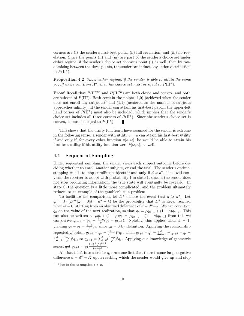
Proof Recall that P pΠSSq and P pΠPRq are both closed and convex, and bothare subsets of P pΠ˚q. Both contain the points (1,0) (achieved when the senderdoes not enroll any subjects)3 and (1,1) (achieved as the number of subjectsapproaches infinity). If the sender can attain his first-best payoff, the upper-lefthand corner of P pΠ˚q must also be included, which implies that the sender’schoice set includes all three corners of P pΠ˚q. Since the sender’s choice set isconvex, it must be equal to P pΠ˚q.

This shows that the utility function I have assumed for the sender is extremein the following sense: a sender with utility v “ a can attain his first best utilityif and only if, for every other function vpa, ωq, he would be able to attain hisfirst best utility if his utility function were vpω, aq, as well.

4.1 Sequential SamplingUnder sequential sampling, the sender views each subject outcome before de-ciding whether to enroll another subject, or end the trial. The sender’s optimalstopping rule is to stop enrolling subjects if and only if d ě d˚. This will con-vince the receiver to adopt with probability 1 in state 1, since if the sender doesnot stop producing information, the true state will eventually be revealed. Instate 0, the question is a little more complicated, and the problem ultimatelyreduces to an example of the gambler’s ruin problem.

To facilitate the comparison, let D˚ denote the event that d ě d˚. Letqk “ PrpD˚c|ω “ 0|d “ d˚ ´ kq be the probability that D˚ is never reachedwhen ω “ 0, starting from an observed difference of d “ d˚´k. We can conditionqk on the value of the next realization, so that qk “ ρqk`1 ` p1´ ρqqk´1. Thiscan also be written as ρqk ` p1 ´ ρqqk “ ρqk`1 ` p1 ´ ρqqk´1; from this wecan derive qk`1 ´ qk “

1´ρρ pqk ´ qk´1q. Notably, this applies when k “ 1,

yielding q2 ´ q1 “1´ρρ q1, since q0 “ 0 by definition. Applying the relationship

repeatedly, obtain qk`1 ´ qk “ p1´ρρ q

kq1. Then qk`1 ´ q1 “řki“1 “ qi`1 ´ qi “

řki“1p

1´ρρ q

iq1, so qk`1 “řki“0p

1´ρρ q

iq1. Applying our knowledge of geometric

series, get qk`1 “ q11´p 1´ρρ q

k`1

1´ 1´ρρ

.

All that is left is to solve for q1. Assume first that there is some large negativedifference d “ d˚ ´K upon reaching which the sender would give up and stop

3due to the assumption z ą µ.

10

enrolling subjects. Then it would be true that qK “ 1. We would also have

1 “ qK “ q11´p 1´ρρ q

K

1´ 1´ρρ

. This tells us that q1 “1´ 1´ρ

ρ

1´p 1´ρρ qK, so qk “

1´p 1´ρρ qk

1´p 1´ρρ qK. As

we let K Ñ8, we get qk Ñ 1´ p 1´ρρ qk.

From this, we can conclude that the probability of NOT reaching d ě d˚

when ω “ 0 and starting with an initial difference of 0 is given by qd˚ “

1 ´ p 1´ρρ qd˚ . Thus when ω “ 0 the probability of successfully persuading the

receiver using sequential sampling is p 1´ρρ qd˚ .

Thus the value of sequential sampling to the sender is given by V wpρq “

µ` p1´ µqp 1´ρρ q

S

logp1´µµ

z1´z

q

logpρ

1´ρq

W

.We are interested in the limit as ρ Ñ` .5. Note that in the limit, d˚ “

Q

logp z1´z q

logp ρ1´ρ q

U

Ñ` 8, and so I will drop the ceiling term in what follows.

Write limρÑ`.5 µ`p1´µqp1´ρρ q

logp1´µµ

z1´z

q

logpρ

1´ρq“ µ`p1´µqplimρÑ`.5p

1´ρρ q

logp1´µµ

z1´z

q

logpρ

1´ρqq

“ µ` p1´ µqp limρÑ`.5

rp1´ ρ

ρq

1logp

ρ1´ρ

qslogp 1´µµ

z1´z qq.

Note that we can write peyq´y´1

“ e´1. Setting y “ logp 1´ρρ q, this identity

becomes p 1´ρρ q1

logpρ

1´ρq“ e´1. Plugging this in, our limit immediately reduces

to

µ` p1´ µqp limρÑ`.5

re´1slogp 1´µµ

z1´z qq “ µ` p1´ µq

µ

1´ µ

1´ z

z“ µ` µp

1´ z

zq

which is the same as the sender’s first-best payoff under unrestricted Bayesianpersuasion. Defining π˚SSpρq to be the signal that induces the same distributionover receiver posteriors as the sender’s optimal stopping rule for a given ρ, wehave the following theorem.

Theorem 4.3 For all µ, z, limρÑ`.5 vpp0pπ˚SSpρqq, p1pπ

˚SSpρqqq “ µ ` µp 1´zz q

under sequential sampling.

This requires that ppπ˚SSpρqq converges to the sender’s first-best point in Π˚.Since this point lies on the same receiver indifference curve as (1,0), the followingcorollary follows.

Corollary 4.4 Under sequential sampling, limρÑ`.5 upp0pπ˚SSpρqq, p1pπ

˚SSpρqqq “

0.

4.2 Pre-RegistrationUnder pre-registration, the sender commits to a non-negative integer samplesize n before viewing any subject outcomes, and has the ability to randomize

11

over sample sizes. Since every randomized trial design is weakly dominated bya trial design without randomization, the sender can restrict his attention tosignals associated with integer choices of n. Accordingly, for the remainder ofthis section I will refer to the sender’s choice of signal π interchangeably withhis choice of sample size n.

Unlike under sequential sampling, calculating the value of an optimal signalto the sender under pre-registration is more difficult than it may seem. Thesender’s expected utility given a sample size of n is

vpppnqq “ µp1pnq ` p1´ µqp1´ p0pnqq

“ µnÿ

x“x˚

ˆ

n

x

˙

ρxp1´ ρqn´x ` p1´ µqnÿ

x“x˚

ˆ

n

x

˙

ρn´xp1´ ρqx,

where again x˚ “Q

d˚`n2

U

and d˚ “logp

zp1´µqµp1´zq q

logp ρ1´ρ q

. Consider the abstracted extreme

case where ρ “ .5 and x˚ is finite.4 Then the sender’s value becomes vpnq “p.5qn

řnx“x˚

`

nx

˘

. There is no hypergeometric expression for the partial sumof binomial coefficients5. Here the sender’s problem is slightly different thanjust a sum of binomial coefficients, and there are some methods for evaluatingother hypergeometric partial sums (e.g. Petkovsek, Wilf, and Zeilberger 1996),so there may exist a closed form expression for the sender’s value. For now,though, I will focus on approaches which do not require us to evaluate thesender’s value function.

Lemma 4.5 For all µ, z, ρ, n, p0pnq ě p1pnq.

Proof Fix n, µ, z, ρ. We can write

p1pnq “ Prpd ě d˚|n, ω “ 1q,

p0pnq “ Prpd ď ´d˚|n, ω “ 0q ` Prpd˚ ą d ą ´d˚|n “ n, ω “ 0q.

By symmetry, Prpd ě d˚|n “ n, ω “ 1q “ Prpd ď ´d˚|n “ n, ω “ 0q. Thusp0pnq ě p1pnq for arbitrary µ, z, ρ, n.

The following graphs depict this bound, as well as the receiver’s indifferencecurve associated with no revelation, the sender’s indifference curve associatedwith full revelation, and the sender’s pre-registration choice set, when µ “

.3, z “ .5, for ρ “ .68, ρ “ .71, and ρ “ .70001, respectively.4I say this example is “abstracted” because, by definition, as ρÑ .5, x˚ Ñ8.5“the indefinite sums

řK0k“0

`nk

˘

cannot be expressed in simple hypergeometric terms in K0

(and n)” (Petkovsek, Wilf, and Zeilberger 1996).

12

13

Note that this bound can be approached as ρ Ñ` .7. Thus, there is asequence of tρu for which the receiver’s utility approaches his baseline utilityunder pre-registration as well. However, unlike under sequential sampling, wherereceiver utility vanishes for very small ρ (and thus very large sample sizes), underpre-registration receiver utility vanishes when ρ is so large that the sender’soptimal sample only enrolls one subject.

In fact, for any µ ă .5 and ρ is sufficiently large, such a one-subject trial isthe sender’s optimal trial under pre-registration. To calculate the smallest valueof ρ for which the receiver will be willing to adopt after seeing only one positiveoutcome, I set z “ µρ

µρ`p1´µqp1´ρq , multiply to obtain µρ “ zpµρ`p1´µqp1´ρqq,combine terms to obtain p1 ´ zqµρ “ zp1 ´ µqp1 ´ ρq, divide to obtain ρ “zp1´µqp1´zqµ p1 ´ ρq, add to obtain ρp1 ` zp1´µq

p1´zqµ q “zp1´µqp1´zqµ , and divide to obtain

ρ “zp1´µqp1´zqµ

1`zp1´µqp1´zqµ

.

Then when ρ ązp1´µqp1´zqµ

1`zp1´µqp1´zqµ

and the sender only enrolls one subject, the re-

sulting trial will have p0 “ p1, found at the northwestern corner of his feasibleset. When µ ă .5, the sender’s indifference curves are steeper than the bounddefined by the line p0 “ p1, and so the sender will prefer this northwestern pointto any other point in his feasible set. I formalize this intuition in the followingproposition

Proposition 4.6 When µ ă .5 and ρ ązp1´µqp1´zqµ

1`zp1´µqp1´zqµ

, the sender’s optimal trial

14

under pre-registration enrolls only one subject.

Proof When ρ ązp1´µqp1´zqµ

1`zp1´µqp1´zqµ

, if the sender enrolls one subject in his trial, then the

receiver will adopt if the outcome is good, and reject if the outcome is bad. Asa result, the probability of the receiver choosing correctly is ρ in either state, sop0p1q “ ρ “ p1p1q. Note that this lies exactly on the bound defined by the linep0 “ p1. Recall that the sender’s expected payoff is vppq “ µp1`p1´µqp1´p0q.Since p0pnq ě p1pnq, choosing a sample size n ą 1 can have one of two effectson p0, p1: either (i) p0pnq “ p1pnq or (ii) p0pnq ě p1pnq. If (i) is true, thenadding the additional n´1 subjects to the trial has the effect of increasing bothp0 and p1 by the same amount (and we know they must have increased sincethe receiver makes more accurate decisions with more information). However,given the sender’s expected payoff of vppq “ µp1`p1´µqp1´ p0q, when µ ă .5,increasing both p0 and p1 by the same positive amount can only lower thesender’s expected payoff. Then if (ii) is true, we must have p0 increase by evenmore than p1, which similarly can only lower the sender’s expected payoff. Thusfor any sample size n ě 1, the sender’s expected payoff is maximized by choosingn “ 1.

As ρÑ`

zp1´µqp1´zqµ

1`zp1´µqp1´zqµ

, the receiver becomes less and less certain about her decision.

In the limit where ρ “zp1´µqp1´zqµ

1`zp1´µqp1´zqµ

, upon seeing a good outcome, the receiver is

exactly indifferent between adopting and rejecting the sender’s treatment. Thus,the receiver is no better off than she was before seeing the sender’s trial, whenshe would choose to reject with probability 1. Defining π˚PRpρq to be the sender’soptimal trial under pre-registration given ρ, we have the following corollary.

Corollary 4.7 When µ ă .5, limρÑ`

zp1´µqp1´zqµ

1`zp1´µqp1´zqµ

upp0pπ˚PRpρqq, p1pπ

˚PRpρqqq “ 0

Note that in this case, pre-registration is worse for the receiver than sequentialsampling: under pre-registration she will only see one subject outcome, butunder sequential sampling she may see further information.

The flip side of this is that when µ ą .5, the sender’s indifference curves areless steep than the bound graphed by p0 “ p1, and so the sender strictly prefersthe northeastern corner of his feasible set. Thus when µ ą .5, full revelation isoptimal for the sender. This is formalized in the following proposition.

Proposition 4.8 If µ ą .5, then for all z and ρ, full revelation (the limit asnÑ8) is the sender’s unique optimal choice under pre-registration.

Proof The sender’s payoff is the probability of receiver adoption. Write vppq “µp1 ` p1´ µqp1´ p0q. Consider the following maximization problem:

maxpp0,p1qPr0,1sˆr0,1s

µp1 ` p1´ µqp1´ p0q

15

s.t. p0 ´ p1 ě 0

and observe that as long as µ ą 1 ´ µ (i.e. µ ą .5), the unique solution ispp0, p1q “ p1, 1q. Since the sender’s choice set P pΠPRq is a subset of the choiceset here (by Lemma 4.5), and p1, 1q P P pΠPRq (full revelation is attained in thelimit as nÑ8, and P pΠPRq is closed), this implies that under pre-registration,full revelation is the sender’s unique optimal choice when µ ą .5.

The following proposition provides a bound on p0 under pre-registration.

Proposition 4.9 For all µ, z, ρ, n, p0pnq ě 1´ 1

1`zp1´µqµp1´zq

.

Proof For any history h “ ps1, s2, ..., snq of subject outcomes that would causethe receiver to adopt the sender’s product, there is a “mirrored” history, inwhich all subject outcomes are reversed, after seeing which the receiver wouldreject the sender’s product. Consider a history h1 which is identical to h exceptthat one subject’s good outcome in h is replaced with one bad outcome for thatsubject in h1. When ω “ 0, history h1 is more likely than history h by a factor ofρ

1´ρ . This is because in the bad state, a bad subject outcome is more likely thana good subject outcome by a factor of ρ

1´ρ . Similarly, replacing a bad outcomewith a good outcome multiplies the likelihood of the history by a factor of 1´ρ

ρ .Replacing one good outcome with a bad outcome and one bad outcome with agood outcome does not affect the likelihood of the history. Since any historyh which leads the receiver to adopt must have at least d˚ more good outcomethan bad outcome, the mirrored history which reverses each subject outcomemust be more likely than history h by a factor of at least p ρ

1´ρ qd˚ .

This yields the inequality p0 ě pρ

1´ρ qd˚p1 ´ p0q. We can then re-write

1 “ p1 ´ p0q ` p0 as 1 ě p1 ´ p0q ` pρ

1´ρ qd˚p1 ´ p0q. Solving for p1 ´ p0q, get

p1´ p0q ď1

1`p ρ1´ρ q

d˚, and so p0 ě 1´ 1

1`p ρ1´ρ q

d˚.

Note that lowering d˚ leads to a smaller quantity being subtracted, which

loosens the bound, and recall that d˚ “R

logpzp1´µqµp1´zq q

logp ρ1´ρ q

V

. Thus we can write

p0 ě 1´1

1` p ρ1´ρ q

logpzp1´µqµp1´zq

q

logpρ

1´ρq

.

Simplifying the denominator, write p ρ1´ρ q

logpzp1´µqµp1´zq

q

logpρ

1´ρq“ pp

ρ1´ρ q

1logp

ρ1´ρ

qqlogp

zp1´µqµp1´zq q “

elogpzp1´µqµp1´zq q “

zp1´µqµp1´zq , where the second to last inequality is due to the identity

peyqp1yq “ e, with y “ logp ρ1´ρ q. Thus we have the bound p0 ě 1 ´ 1

1`zp1´µqµp1´zq

.

16

5 ConclusionWe have seen that in a simple model of trial design, requiring the sender topre-register his sample size can have large effects on receiver welfare and the setof attainable outcomes. Under the sequential sampling regime, as the informa-tion generated by each subject vanishes, the sender can approach his first-bestBayesian persuasion payoff, and the receiver’s payoff approaches her first-worst.Under the pre-registration regime, we have seen that there is a bound on the falsepositive rate of the sender’s test, and if the good state is at least as likely as thebad state ex ante, the sender will choose to reveal the state fully.Interestingly,it is not always true that the receiver is better off under pre-registration; whenµ ă .5 and ρ is sufficiently large, the sender will only pre-register one subject,which is worse for the receiver than sequential sampling. Thus we have thefollowing takeaway: when µ ă .5, and when each subject outcome is very un-informative, pre-registration leads to more informative trials, but when subjectoutcomes are very informative, sequential sampling leads to more informativetrials.

Further questions remained to be studied. While the receiver prefers pre-registration when subject outcomes are highly uninformative and sequentialsampling when subject outcomes are highly informative, it is still unclear whatwe can say about intermediate values of ρ. It would also be interesting to seea more general model where the state space need not be binary, and subjectoutcomes need not be Bernoulli.

6 ReferencesBrocas, Isabelle, and Juan D. Carrillo. "Influence through ignorance." TheRAND Journal of Economics 38.4 (2007): 931-947.

Henry, Emeric, and Marco Ottaviani. 2019. "Research and the Approval Pro-cess: The Organization of Persuasion." American Economic Review, 109 (3):911-55.

Kamenica, E., Gentzkow, M.: Bayesian persuasion. Am. Econ. Rev. 101,2590–2615 (2011)

Kaplan, R. & Irvin, V. PLoS ONE 10, e0132382 (2015)

Morris, Stephen, and Philipp Strack. 2019. “The Wald Problem and the Equiv-alence of Sequential Sampling and Static Information Costs.” Unpublished.

Petkovšek, Marko., Herbert S. Wilf, and Doron. Zeilberger. A=B / MarkoPetkovšek, Herbert S. Wilf, Doron Zeilberger. Wellesley, MA: A K Peters, Ltd.,1996. Print.

17