Additive and multiplicative effects network models

Peter D. Hoff

Department of Statistical Science

Duke University

July 24, 2018

Abstract

Network datasets typically exhibit certain types of statistical dependencies, such as within-

dyad correlation, row and column heterogeneity, and third-order dependence patterns such as

transitivity and clustering. The first two of these can be well-represented statistically with a

social relations model, a type of additive random effects model originally developed for contin-

uous dyadic data. Third-order patterns can be represented with multiplicative random effects

models, which are related to matrix decompositions commonly used for matrix-variate data

analysis. Additionally, these multiplicative random effects models generalize other popular la-

tent variable network models, such as the stochastic blockmodel and the latent space model.

In this article we review a general regression framework for the analysis of network data that

combines these two types of random effects and accommodates a variety of network data types,

including continuous, binary and ordinal network relations.

Keywords: Bayesian, factor model, generalized linear model, latent variable, matrix decomposi-

tion, mixed effects model.

1 Introduction

Network data provide quantitative information about relationships among objects, individuals or

entities, which we refer to as nodes. Most network data quantify pairwise relationships between

nodes. A pair of nodes is referred to as a dyad, and a quantity that is measured or observed for

multiple dyads is called a dyadic variable. Common sample spaces for dyadic variables include

continuous, discrete, dichotomous and ordinal spaces, among others. Examples of dyadic variables

1

arX

iv:1

807.

0803

8v1

[st

at.M

E]

20

Jul 2

018

include quantitative measures of trade flows between countries, communications among people,

binding activity among proteins, and structural connections among regions of the brain, to name

just a few.

Measurements of a dyadic variable on a population of n nodes may be summarized with a

sociomatrix, an n × n square matrix Y with an undefined diagonal, where entry yi,j denotes the

value of the relationship between nodes i and j from the perspective of node i, or in the direction

from i to j. Analysis of an observed sociomatrix Y often proceeds in the context of one or more

statistical models, with which a data analyst may evaluate competing theories of network formation,

describe patterns in the network, estimate effects of other variables on dyadic relations, or impute

missing values.

While most of the dyadic variables I have encountered are not dichotomous in their raw form,

much of the statistical literature has focused on binary network data for which the sociomatrix Y

can be viewed as the adjacency matrix of a graph. Many statistical random graph models are mo-

tivated by intuitive, preconceived notions of how networks may form, particularly social networks.

For example, preferential attachment models view an observed network as the end result of a so-

cial process in which nodes are sequentially introduced into a population of existing nodes (Price,

1976). As another example, the parameters in the types of exponential family graph models that

are commonly used have interpretations as node-level preferences for certain relationship outcomes

(Wasserman and Pattison, 1996).

An alternative approach is to build a statistical model for Y based on its inherent structure as

a sociomatrix, that is, as a data matrix whose row labels are the same as its column labels. Such

an approach can build upon familiar, well-developed statistical methodologies such as ANOVA,

linear regression, matrix decompositions, factor analysis and linear and generalized linear mixed

effects models, and can be applied to a wide variety of dyadic data types. In this article, we

review such a framework for network data analysis using these tools, starting with simple ANOVA-

style decompositions of sociomatrices and ending with additive and multiplicative random effects

regression models for continuous, binary, ordinal and other types of dyadic network data.

In the next section we review an ANOVA-style decomposition of a sociomatrix known as the

social relations model (SRM) (Warner et al., 1979; Wong, 1982), which corresponds to a particular

Gaussian additive random effects model for network data. An extension of this model that includes

2

covariates is also developed, which we call the social relations regression model (SRRM). The SRM

and SRRM are able to describe network variances and covariances, but are unable to describe

third-order dependence patterns such as transitivity, balance, or the existence of clusters of nodes

with high subgroup densities of ties. In Section 3 we discuss how such patterns can be represented

by a multiplicative latent factor model, in which the relationship between two nodes depends on

the similarity of their unobserved latent factors. From a matrix decomposition perspective, this

motivates the use of an “additive main effects, multiplicative interaction” (AMMI) matrix model

(Gollob, 1968; Bradu and Gabriel, 1974). Combining an AMMI model with a social relations

covariance model yields what we call an additive and multiplicative effects (AME) network model.

These AME models are built from linear regression, random effects models and matrix decom-

position - methods which are most appropriate for continuous data consisting of a signal of interest

plus Gaussian noise. In contrast, many dyadic variables are discrete, ordinal, binary or sparse. In

Section 4 we extend the AME framework to accommodate these and other types of dyadic variables

using a Gaussian transformation model. In Section 5 we compare the multiplicative effects compo-

nent of an AME model with two other latent variable network models, the stochastic blockmodel

(Nowicki and Snijders, 2001) and the latent space model (Hoff et al., 2002). We review results

showing that these latter two models can be viewed as submodels of the multiplicative effects

model. Connections to exponentially parameterized random graph models (ERGMs) (Wasserman

and Pattison, 1996) are also discussed. Section 6 presents a Markov chain Monte Carlo algorithm

for Bayesian model fitting of a hierarchy of AME network models. A discussion follows in Section

7.

2 Social Relations Regression

2.1 ANOVA and the Social Relations Model

Numeric sociomatrices typically exhibit certain statistical features. For example, it is often the case

that values of the dyadic variable in a given row of the sociomatrix are correlated with one another,

in the sense that high and low values are not equally distributed among the rows, resulting in

substantial heterogeneity of the row means of the sociomatrix. Such heterogeneity can be explained

by the fact that the relations within a row all share a common “sender,” or row index. If sender i1

3

is more “sociable” than sender i2, we would expect the values in row i1 to be larger than those in

row i2, on average. In this way, heterogeneity of the nodes in terms of their sociability contributes

to an across-row variance of the row means of the sociomatrix. Similarly, nodal heterogeneity in

“popularity” contributes to the across-column variance of the column means.

A classical approach to evaluating across-row and across-column heterogeneity in a data matrix

is the ANOVA decomposition. A statistical model based on the ANOVA decomposition posits that

the variability of the yi,j ’s around some overall mean µ is well-represented by additive row and

column effects:

yi,j = µ+ ai + bj + εi,j . (2.1)

In this model, heterogeneity among the ai’s and bj ’s gives rise to observed heterogeneity in the row

means and column means of the sociomatrix, respectively.

While straightforward to implement, a classical ANOVA analysis ignores a fundamental char-

acteristic of dyadic data: Each node appears in the dataset as both a sender and a receiver of

relations, or equivalently, the row and column labels of the data matrix refer to the same set of

nodes. In the context of the ANOVA model, this means that each node i has two additive effects:

a row effect ai and a column effect bi. Since each pair of effects (ai, bi) shares a node, a correlation

between the vectors (a1, . . . , an) and (b1, . . . , bn) may be expected. Additionally, each dyad {i, j}

has two outcomes, yi,j and yj,i. As such, the possibility that εi,j and εj,i are correlated should be

considered.

We illustrate these phenomena empirically with a sociomatrix of export data among n = 30

countries. Here, yi,j is the 1990 export volume from country i to country j, in log billions of dollars.

For each country i = 1, . . . , n, ai the ith row mean minus the grand mean µ of the sociomatrix,

and bi is the ith column mean minus µ. The left panel of Figure 1 shows that these row and

column effects are strongly correlated - countries with large export volumes typically have larger

than average import volumes as well. A scatterplot of εi,j = yi,j−(µ+ ai+ bj) versus εj,i in the right

panel of the plot indicates a strong dyadic correlation, even after controlling for country-specific

heterogeneity in export and import volumes.

The standard ANOVA model of a data matrix quantifies row variation, column variation and

residual variation. However, the ANOVA model does not quantify the sender-receiver or dyadic

correlations that are apparent from the figure, and that are present in most other dyadic datasets I

4

−0.5 0.0 0.5 1.0 1.5

−0.

50.

00.

51.

01.

5

ai

b i^

ARG

AUL

BEL

BNG

BRA

CAN

CHN

COLEGY

FRN

INDINS

IRN

ITA

JPN

MEX

NTH

PAK

PHIPOL

ROK

SAFSAU

SPN

SWD

TAW

THITUR

UKG

USA

●●

●

●

●●

●●

●

●●

●

●

●

●

●

●●●

●

●●

●●

●

● ●

● ●

●

●

●

● ●

●

●●

●

●

●

●

●

●

●

●

●●

●

●

●●

●●

●

●

● ●●

●●

●●

●●

●●

●

●

●

●

●

●

●

●

●●

●

●

●●

●●

●●

●

●

●

●●

●

●●

●

●●

●

●●●

●

●

●

●

●●●

●

●●

●

●

●

● ●

●

●

●

●●●●●

●●

●●●

●●●

●

● ●● ●●● ●●●●● ●

●

●

●●

●●● ●●

●●

●●●

●

●●

●

●●●

●

●●

●●

●●●

●

●

●

●

●●

●

●

●●

●

●●

●

●

●

●

●

●●

●

●

●●●

●

●●

●

●

●

●

●●

●

●●

●

●

●

●●●

●

●

●

●

●●●

●

●●

●

●

●

● ●

●

●

●

●●

●

●

●●

●

●

●●

●●

●

●

●

●● ●

●

●●

●

●

●●

●

●

●

●●

●

●

●● ●

●

●●●

●

●

●●

●

●●

●

●● ●

●

●

●

●

●

●

●● ●

●

●

●●

● ● ●

●

● ●

●● ●●

●●●●

●●

●●●

●●●●●

●

●

●

●●

●

●●

●

●●

●

●

●●

●●●

●

●●

●●

●

●

●●

● ●

●●

●●

●●

●●

●

●

●●●

●●

●●●●

●

●●●

● ●

●

●

●

●●

●

●

●

●●

●

●

●

●●

●●●

●

●

●

●

●●

●

●

●

●●

●

●

●

●

●

●

●

●

●

●

●●

●

●

●

●●

●●

●

●

●

●

●●

● ●

●

●

●

●

●

●

●●

● ●

●

●

●

●

●

●●●

●

●●

●●●

●

●●

●

●●●●

●

●

●●

●

● ●● ●●●

●

●● ●

●

●

●● ●

●

●

● ●

●●

●●

●

●

●

●●

●

●

●●●

●●

●

●●●

●●

●

●

●●

●

●●

●

●●

● ●

●

●

●●

●

●

●●●●●

●

●●●

●

●

●●●●●● ●

●

●

●●

●

●

●●

● ●

●

●

●●

●●

●●●

●●

●

● ●

●●

●

●●

●

●

●● ●

●

●

●

●

●

●●

●

●

●●

●

●

●

●

●

●

●

●

●

●

●●

●

●●

●

●

●●

●

●●●

●●

●●

●●

●

●●

●

●

●●

●

●●●● ●

●●

●●

●●

●

●●

●

●

●

●●

●●●

●

●●●

●

●

●●●

●

●

●●●

●●

●

●

●●

●

●

●●

● ●

●●

●

●●●

●

●

●●

●●

●

●

●●●

●●

●

●

●

●●

●

●●●● ●●

●

●●●●

●●

●

●●

●

●

●●●

●●

●

●

●●

●

●

●●

●

●

●●

●●

●

●●

●

●●

●

●

●

●●●

●●

●

●●

●

●

●

●

●

●●

●

●●

●●

●●

●

●

●●●●● ●●●

●●

●

●●

●

●● ●

●

●●

●

●●

●●●

●●

●

●●

●●

●

●

●●

●●

●● ●

●●

●

●

●●

●

●

●●

●

●

●●

●

●

●

●

●●

●

●

●●

●●

●●

●

●

●

●

●

●

●

●

●

●

●

●

●●

●

●

●

●

●

●

●

●

●

●

●

● ●

●

●

●

●

−2 −1 0 1 2

−2

−1

01

2

ei, j

e j, i

Figure 1: Left panel: Scatterplot of country-level export effects versus import effects. Right panel:

Scatterplot of dyadic residuals.

have seen. A model that does quantify these correlations, and therefore provides a more complete

description of the sociomatrix, was introduced in the psychometrics literature by Warner et al.

(1979). This more complete model, called the social relations model (SRM), is a random effects

model given by 2.1 but with the additional assumptions that

Var[(aibi )] = Σ =

σ2a σab

σab σ2b

Var[(εi,jεj,i )] = σ2

1 ρ

ρ 1

, (2.2)

with effects otherwise being independent. Straightforward calculations show that under this random

effects model, the variance of the relational variable is Var[yi,j ] = σ2a + 2σab + σ2b + σ2, and the

covariances among the relations are

Cov[yi,j , yi,k] = σ2a (within-row covariance)

Cov[yi,j , yk,j ] = σ2b (within-column covariance)

Cov[yi,j , yj,k] = σab (row-column covariance)

Cov[yi,j , yj,i] = 2σab + ρσ2 (row-column covariance plus reciprocity)

with all other covariances between elements of Y being zero. We refer to this covariance model

as the social relations covariance model. Unbiased moment-based estimators of µ, Σ, σ2 and ρ

are derived in Warner et al. (1979), and standard errors for these estimators are obtained in Bond

5

IID SRRM AME

regressor β se(β) t-ratio β se(β) t-ratio β se(β) t-ratio

exporter polity 0.015 0.004 4.166 0.015 0.016 0.934 0.012 0.016 0.782

importer polity 0.022 0.004 6.070 0.022 0.016 1.419 0.018 0.015 1.190

exporter GDP 0.411 0.021 19.623 0.407 0.095 4.302 0.346 0.103 3.373

importer GDP 0.398 0.020 19.504 0.397 0.094 4.219 0.336 0.103 3.250

distance -0.057 0.004 -13.360 -0.064 0.005 -11.704 -0.041 0.004 -10.970

Table 1: Parameter estimates and standard errors from the trade data using a normal linear

regression model with i.i.d. errors, a SRRM, and an AME model.

and Lashley (1996). Under the additional assumption that the random effects are jointly normally

distributed, Wong (1982) provides an EM algorithm for maximum likelihood estimation, Gill and

Swartz (2001) develop a Bayesian method for parameter estimation, and Li and Loken (2002)

discuss connections to models in genetics and extensions to repeated-measures dyadic data.

2.2 Social relations regression models

Often we wish to quantify the association between a particular dyadic variable and some other

dyadic or nodal variables. Useful for such situations is a type of linear mixed effects model we refer

to as the social relations regression model (SRRM), which combines a linear regression model with

the covariance structure of the SRM as follows:

yi,j = β>xi,j + ai + bj + εi,j , (2.3)

where xi,j is a p-dimensional vector of regressors and β is a vector of regression coefficients to be

estimated. The vector xi,j may contain variables that are specific to nodes or pairs of nodes. For

example, we may have xi,j = (xr,i,xc,j ,xd,i,j) where xr,i is a vector of characteristics of node i as

a sender or row object, xc,j is a vector of characteristics of node j as a receiver or column object,

and xd,i,j is a vector of characteristics of the ordered pair (i, j).

We illustrate the use of the SRRM with a more detailed analysis of the international trade

dataset described above. This dataset also includes several other variables, such as country-specific

measures of gross domestic product (GDP) and polity (a measure of citizen access to government),

as well as the geographic distance between pairs of county capitals. Our objective in this example

6

is to quantify the relationship between trade and polity after controlling for the effects of GDP and

geographic distance. We first do so with a naive ordinary linear regression model of the form

yi,j = β0 + βr,1polityi + βr,2gdpi + βc,1polityj + βc,2gdpj + βddistancei,j + εi,j ,

where polityi is a measure of country i’s polity score on a scale from 1 to 10, gdpi is the log GDP

of country i in dollars, distancei,j is the log distance in miles between capitals of countries i and

j, and the εi,j ’s are assumed to be i.i.d. mean-zero error terms. This model is a “gravity model”

of trade (Isard, 1954; Bergstrand, 1985), where trade flow is analogous to a gravitational force

between countries, and GDP plays the role of mass. Gravity models of this type are widely used

to empirically evaluate different theories of international trade (Baier and Bergstrand, 2009).

Regression parameter estimates and standard errors assuming an i.i.d. error model are given in

the first column of Table 1. Based upon the ratio of parameter estimates to standard errors, we

would conclude that the hypothesis of no polity effects is inconsistent with an i.i.d. error model.

However, while technically valid, this conclusion is not particularly interesting given that we expect

row, column and dyadic dependence for network data such as these, and thus doubt the i.i.d. error

model a priori. More interesting is an evaluation of whether or not the hypothesis of no polity

effects is consistent with a social relations covariance model. The parameter estimates and standard

errors for the SRRM in the second column of the table indicate that indeed it is: the parameter

estimates of the polity effects are not substantially larger than their standard errors.

3 Multiplicative Effects Models

While more reasonable than an ordinary regression model, SRRMs applied to many datasets often

exhibit substantial lack of fit. In particular, it is often observed that real networks exhibit patterns

of dependence among triples of nodes such as transitivity, balance and clustering (Wasserman and

Faust, 1994). For example, in the context of fitting a regression model, the notion of balance would

correspond to there generally being a higher-than expected relationship (i.e. a positive residual)

between nodes j and k if that between i and j and i and k were both also higher than expected.

Such patterns can be quantified with summary statistics such as∑

i,j,k εi,j εj,k εk,i, where εi,j is a

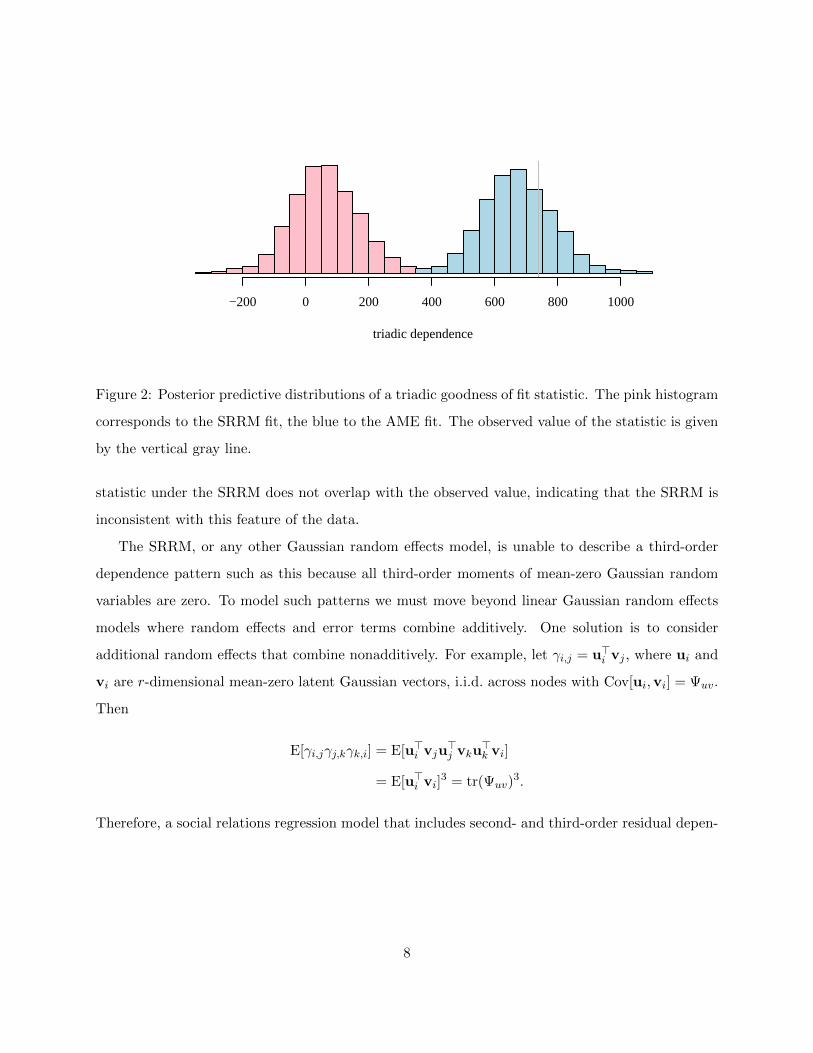
residual from a least-squares fit. Figure 2 displays the posterior predictive distribution of this

statistic from a Bayesian fit of the SRRM to the trade data. The predictive distribution of this

7

triadic dependence

−200 0 200 400 600 800 1000

Figure 2: Posterior predictive distributions of a triadic goodness of fit statistic. The pink histogram

corresponds to the SRRM fit, the blue to the AME fit. The observed value of the statistic is given

by the vertical gray line.

statistic under the SRRM does not overlap with the observed value, indicating that the SRRM is

inconsistent with this feature of the data.

The SRRM, or any other Gaussian random effects model, is unable to describe a third-order

dependence pattern such as this because all third-order moments of mean-zero Gaussian random

variables are zero. To model such patterns we must move beyond linear Gaussian random effects

models where random effects and error terms combine additively. One solution is to consider

additional random effects that combine nonadditively. For example, let γi,j = u>i vj , where ui and

vi are r-dimensional mean-zero latent Gaussian vectors, i.i.d. across nodes with Cov[ui,vi] = Ψuv.

Then

E[γi,jγj,kγk,i] = E[u>i vju>j vku

>k vi]

= E[u>i vi]3 = tr(Ψuv)

3.

Therefore, a social relations regression model that includes second- and third-order residual depen-

8

dencies is given by

yi,j = β>xi,j + u>i vj + ai + bj + εi,j (3.1)

(u1,v1), . . . , (un,vn) ∼ i.i.d. N2r(0,Ψ)

(a1, b1), . . . , (an, bn) ∼ i.i.d. N2(0,Σ)

{(εi,j , εj,i) : i < j} ∼ i.i.d. N2(0, σ2( 1 ρρ 1 )).

We call such a model an additive and multiplicative effects model (AME). Specifically, we refer to

the model given by (3.1) as a Gaussian AME, since the observed data are conditionally Gaussian,

given β and the multiplicative effects. A rudimentary multiplicative effects model appeared in Hoff

et al. (2002), along with some other nonadditive random effects models. A symmetric multiplicative

effects model was combined with the social relations covariance model in Hoff (2005), and versions

of (3.1) were studied and developed in Hoff (2008, 2009) and Hoff et al. (2013).

The matrix form of this model can be expressed as

Y = M + a1> + 1b> + UV> + E,

where mi,j = β>xi,j , a = (a1, . . . , an), b = (b1, . . . , bn) and U and V are n × r matrices with ith

rows equal to ui and vi respectively, with r being the length of each of these latent vectors. This

represents the deviations of Y from the linear regression model M as the sum of a rank-1 matrix of

row effects, a rank-1 matrix of column effects, a rank-r matrix UV> and a noise matrix E. Absent

a covariance model for the node-specific effects or dyadic residuals, this representation is essentially

a special case of an additive main effects, multiplicative interaction (AMMI) model (Gollob, 1968;

Bradu and Gabriel, 1974), a class of matrix models developed in the psychometric and agronomy

literature for data arising from two-way layouts with no replication. Since sociomatrices have

additional structure - the row factors are the same as the column factors - our random effects

version of the AMMI model includes the SRM covariance model for the ai’s, bi’s and εi,j ’s, in

addition to a random effects model for ui and vi to represent possible third-order dependencies in

the sociomatrix. We refer to this model as an additive and multiplicative effects model, or AME

model for dyadic network data.

To illustrate the how the inclusion of multiplicative effects improves model fit, we obtain the

posterior predictive distribution of the triadic goodness-of-fit statistic∑

i,j,k εi,j εj,k εk,i under an

9

−0.6 −0.4 −0.2 0.0 0.2 0.4

−0.

6−

0.2

0.2

0.4

additive row effects

addi

tive

colu

mn

effe

cts

ARGAUL

BEL

BNG

BRA

CANCHNCOLEGY

FRN

IND

INSIRNITA

JPN

MEX

NTH

PAK

PHI

POL

ROK

SAF

SAU

SPN SWD

TAW

THI

TUR

UKG

USA

ARG

AUL

BEL

BNG

BRA

CAN

CHN

COL

EGY

FRN

IND

INS

IRN

ITA

JPN

MEX

NTH

PAK

PHI

POL

ROK

SAF

SAU

SPNSWD

TAWTHI

TUR

UKG

USA

ARG

AUL

BEL

BNG

BRA

CANCHN

COL

EGY

FRN

IND

INS

IRN

ITA

JPNMEX

NTH

PAK

PHI

POL

ROK

SAF

SAU

SPNSWD

TAWTHI

TUR

UKG

USA

Figure 3: Estimates of node-specific effects. The left panel gives additive row effects versus additive

column effects. The plot on the right gives estimates of ui in red and vi in blue for each country

i = 1, . . . , n. The country names indicate the direction of these vectors, and the size of the plotting

text indicates their magnitude. A dashed line is drawn between an export-import pair if their trade

flow is larger than expected based on the other terms in the model.

AME model with two-dimensional multiplicative effects and the same regressors as the SRRM

(polity, GDP and geographic distance). A histogram of this posterior predictive distribution is

given in Figure 2, along with that of the SRRM fit. The posterior predictive distribution obtained

under the AME fit is roughly centered around the observed value of the statistic indicating that,

unlike the SRRM, the AME model is able to describe this third-order residual dependency in the

trade data. Finally, parameter estimates and standard errors for the regression coefficients in this

AME model are given in the third column of Table 1. Parameter estimates are slightly smaller

than those of the SRRM, but the main conclusions remain the same.

From a random effects perspective, the multiplicative effect u>i vj can be viewed as a means

to quantify third order dependence. However, these effects can also be interpreted as representing

omitted regression variables or uncovering group structure among the nodes. This interpretation

is based on the observation that the strength or presence of ties between nodes is often related to

similarities of node-level attributes. For example, suppose for each node i that xi is the indicator

that i is a member of a particular group or has a particular trait. Then xixj is the indicator that

10

i and j are co-members of this group, and this fact may have some effect on their relationship yi,j .

A positive association between xixj and yi,j is referred to as homophily, and a negative association

as anti-homophily. Quantifying homophily on an observed attribute can be done with a SRRM by

creating a dyadic regressor xd,i,j from a nodal regressor xi through multiplication (xd,i,j = xixj) or

some other operation. However, the possibility that not all relevant nodal attributes are included

in a network dataset motivates inclusion of the multiplicative term u>i vj , where ui and vi represent

unobserved latent factors of node i as a sender and receiver of relations, respectively.

These latent factors may be estimated and examined to highlight additional structure in the

data beyond that explained by the SRRM. For example, estimates of the ui’s and vi’s of the rank-2

AME fit to the trade data are displayed in Figure 3. Recall that this model includes polity, GDP

and geographic distance as regressors, in addition to the additive effects and multiplicative latent

factors. The interpretation of the multiplicative factors is that if ui and vj are large and in the

same direction, then nodes i and j tend to have observed trade flows larger than β>xi,j + ai + bj ,

that is, larger than what is predicted by the additive effects alone. As can be seen from the figure,

the estimates of the latent factors from these data highlight some geographically related clustering

of nodes, in particular, a cluster of Pacific rim countries and a cluster of mostly European countries.

These are patterns that, while related to geographic distance, are not well-represented by a single

linear relationship between log-trade and log-distance in the regression model.

4 Transformation models for non-Gaussian networks

On their original scale, many dyadic variables are not well-represented by a model with Gaussian

errors. In some cases, such as with the trade data, a dyadic variable can be transformed so that

the Gaussian AME model is reasonable. In other cases, such as with binary, ordinal, discrete or

sparse variables, no such transformation is available. Examples of such data include measures of

friendship that are binary (not friends/friends) or ordinal (dislike/neutral/like), discrete counts of

conflictual events between countries, or the amount of time two people spend on the phone with

each other. In this section we describe extensions of the Gaussian AME model to accommodate

ordinal dyadic data, where in what follows, ordinal means any outcome for which the possible values

can be put in some meaningful order. This includes discrete outcomes (such as binary indicators or

counts), ordered qualitative outcomes (such as low/medium/high), and even continuous outcomes.

11

The extensions are based on latent variable representations of probit and ordinal probit regression

models.

4.1 Binary and ordinal network data

Let S be the observed sociomatrix for a dyadic variable si,j . The simplest type of ordinal dyadic

variable is a binary variable indicating the presence of some type of relationship between i and j,

so that si,j = 0 or 1 depending on whether a social link is absent or present, respectively. One

approach to quantifying the association between such a binary variable and other variables is with

probit regression, which models the probability of a link between i and j as Φ(β>xi,j), where

Φ is the standard normal CDF. As is well known, the probit regression model has a latent vari-

able representation in which si,j is the binary indicator that some latent normal random variable

yi,j ∼ N(β>xi,j , 1) is greater than zero (Albert and Chib, 1993). An ordinary probit regression

model corresponds to the yi,j ’s being independent, which is generally an inappropriate assumption

for network data. However, a model for binary data that does capture the types of network depen-

dencies discussed in the previous section, such as row and column covariance, dyadic correlation,

and triadic dependence, can be represented via an AME model for the latent yi,j ’s:

yi,j = β>xi,j + u>i vj + ai + bj + εi,j (4.1)

si,j = g(yi,j),

where the ai’s bi’s and εi,j ’s follow the SRM covariance model and g(y) is the binary indicator that

y > 0. Absent the multiplicative term u>i vj , this is basically a generalized linear mixed effects

model. Including the multiplicative term but absent the SRM covariance structure, this model is a

type of generalized bilinear regression (Gabriel, 1998). Including both the multiplicative term and

the SRM covariance structure yields a regression model for binary social network data that can

accommodate second- and third-order dependence patterns.

This probit AME model for binary data extends in a natural way to accommodate ordinal data

with more than two levels. As with binary data, we model the observed sociomatrix S as being

a function of a latent sociomatrix Y that follows a Gaussian AME distribution. Specifically, the

model is the same as in Equation 4.1 but with g being a non-decreasing function. Such a model

may be viewed as a type of Gaussian transformation model (Bickel and Ritov, 1997).

12

One approach to estimation for these models is as follows: For both the probit and ordinal probit

models, observation of S tells us that Y lies in a certain set, say Y ∈ C(S). For the binary probit

model, this set is simply given by C(S) = {Y ∈ Rn×n : sign(yi,j) = sign(2si,j − 1)}, that is, si,j = 1

implies yi,j > 0 and si,j = 0 implies yi,j < 0. For the ordinal probit model, since g is non-decreasing

we have C(S) = {Y ∈ Rn×n : maxi′j′{yi′,j′ : si′,j′ < si,j} < yi,j < mini′j′{yi′,j′ : si,j < si′j′}}. A

likelihood based on the knowledge that Y ∈ C(S) is given by L(θ) = Pr(Y ∈ C(S)|θ) where θ are

the parameters in the Gaussian AME model for Y. While a closed form expression for this likelihood

is unavailable, a Bayesian approach to estimation and inference is feasible via Gibbs sampling by

iteratively simulating θ from its full conditional distribution given Y, then simulating Y from

its conditional distribution given θ but constrained to lie in C(S). More details are presented in

Section 6.

4.2 Censored and ranked nomination data

Data on human social networks are often obtained by asking participants in a study to name and

rank a fixed number of people with whom they are friends. Such a survey method is called a

fixed ranked nomination (FRN) scheme, and is used in studies of institutions such as schools or

businesses. For example, the National Longitudinal Study of Adolescent Health (AddHealth, Harris

et al. (2009)) asked middle and high-school students to nominate and rank up to five members of

the same sex as friends, and five members of the opposite sex as friends.

Data obtained from FRN schemes are similar to ordinal data, in that the ranks of a person’s

friends may be viewed as an ordinal response. However, FRN data are also censored in a complicated

way. Consider a study where people were asked to name and rank up to and including their top

five friends. If person i nominates five people but doesn’t nominate person j, then si,j is censored:

The data cannot tell us whether j is i’s sixth best friend, or whether j is not liked by i at all. On

the other hand, if person i nominates four people as friends but could have nominated five, then

person i’s data are not censored - the absence of a nomination by i of j indicates that i does not

consider j a friend.

A likelihood-based approach to modeling FRN data using an AME model was developed in Hoff

et al. (2013). Similar to the approach for ordinal dyadic data described above, this methodology

treats the observed ranked outcomes S as a function of an underlying continuous sociomatrix Y of

13

affinities that is generated from an AME model. Letting m be the maximum number of nominations

allowed, and coding si,j ∈ {m,m − 1, . . . , 1, 0} so that si,j = m indicates that j is i’s most liked

friend, the FRN likelihood is derived from the following constraints that the observed ranks S tell

us about the underlying dyadic variables Y:

si,j > 0 ⇒ yi,j > 0 (4.2)

si,j > si,k ⇒ yi,j > yi,k (4.3)

si,j = 0 and di < m ⇒ yi,j ≤ 0. (4.4)

Constraint (4.2) indicates that if i ranks j, then i has a positive relation with j (yi,j > 0), and

constraint (4.3) indicates that a higher rank corresponds to a more positive relation. Letting

di ∈ {0, . . . ,m} be the number of people that i ranks, constraint (4.4) indicates that if i could have

made additional friendship nominations but chose not to nominate j, they then do not consider j a

friend. However, if si,j = 0 but di = m then person i’s unranked relationships are censored, and so

yi,j could be positive even though si,j = 0. In this case, all that is known about yi,j is that it is less

than yi,k for any person k ranked by i. In summary, observation of S tells us that Y ∈ C(S) where

C(S) is defined by conditions 4.2 - 4.4. As with the probit and ordinal AME models, Bayesian

inference for this transformation model can proceed by iteratively simulating values of the model

parameters and the unknown values of Y from their full conditional distributions.

5 Comparisons to other models

Two popular categories of statistical network models are exponentially parameterized random graph

models (ERGMs) and latent variables models. Roughly speaking, ERGMs focus on characterizing

global, macro-level patterns in a network, while latent variable models describe local, micro-level

patterns of relationships among specific nodes. The AME class of model can characterize both

global and local patterns, the former via the global parameters {β,Σ,Ψ, σ2, ρ} and the latter via

the node-specific factors {ai, bi,ui,vi : i = 1, . . . , n}.

5.1 Comparisons to ERGMs

An ERGM is a probability model for a binary sociomatrix that includes densities of the form

p(Y) = c(θ) exp(θ · t(Y)), where t(Y) is a vector of sufficient statistics and θ is a parameter to

14

be estimated. Typical applications use a small number of sufficient statistics, often much smaller

than the number of nodes, and in this sense the models describe “global” patterns in the data. An

exception to this is the not-infrequent inclusion of out- and in-degree statistics that can characterize

the differential sociability and popularity of the nodes. For example, one of the first ERGMs to be

widely used and studied was the “p1” model (Holland and Leinhardt, 1981) with density

p(Y) ∝ exp

µ∑i,j

yi,j +∑i

(ai∑j

yi,j + bi∑j

yj,i) + ρ∑i,j

yi,jyj,i

,

which includes as sufficient statistics the total number of ties∑

i,j yi,j , the number of reciprocated

ties∑

i,j yi,jyj,i and the in- and out-degrees {∑

j yi,j ,∑

j yj,i, i = 1, . . . , n}. The parameters in this

model represent roughly the same data features as they do in the SRM: an overall mean of the

relations (µ), heterogeneity in row and column means (the ai’s and bi’s) and dyadic correlation

(ρ). Similarities are also found between the SRRM and the “p2” model developed by van Duijn

et al. (2004). The p2 model extends the p1 model by including regressors (as does the SRRM), and

additionally treats the node-level parameters ai and bi as potentially correlated random effects (as

do the SRM and SRRM).

Holland and Leinhardt (1981) concede that the p1 model is of limited utility due to its inability

to describe more complex forms of dependency such as transitivity or clustering. While inclusion

of appropriate regressors, either in a p2 model or SRRM, can represent some degree of higher-

order dependency, often such models still exhibit lack-of-fit and more complex models are desired.

As described in Section 3, the AME approach is to include a multiplicative latent variable term

u>i vj , that when thought of as a random effect, induces non-zero third order moments in the error

structure. In contrast, the ERGM approach to describing higher-order dependencies is to include

additional sufficient statistics, such as the number of triangles observed in the graph, or the number

of cycles of various lengths (Snijders et al., 2006). Unfortunately, simultaneous inclusion of such

statistics and those that naturally represent degree heterogeneity can lead to model degeneracy

(Handcock, 2003; Hunter and Handcock, 2006).

5.2 Comparison to other latent variable models

While globally inducing third-order dependence among network outcomes, the multiplicative term

u>i vj in the AME model can also be interpreted locally at the micro-level, in that ui and vi describe

15

●

●●

●

●

●

●

●

●●

●●

●

●

●

●

●

●

●

●●

●

●●

●

●● ●

●

●●● ●

●

●

●

●

●●

●

●

●●

●

●●

●

●

●●

●●

●

● ●

●

●

●● ●

●

●

●

●

●●

●

●

●

●

●●

●

●

●

●

●

●●●

●

●●

●

●

●

●●●

●

●

●

●

●●

●

●

●

●

●

●●

●

●●●

●

●

● ●

●

●●●

●

●

● ●●

●

●● ●

●

● ●

●

● ● ●

● ●

●●

●

●●

●●

●

●●

● ●

●

●

●●

●●

●

●

●

●●●

●

●

●●

●●

●

●

●●

●●

●

●

●●

●

●

●

●

●●

●

●

●

● ●

●

●

●●

●

●

●

● ●

● ●●

● ●

●●

●

Figure 4: Two hypothetical networks. The network on the left can be represented by two groups

of stochastically equivalent nodes. The network on the right can be represented by an embedding

of the nodes in two-dimensional Euclidean space.

latent features of node i as a sender and receiver of ties. Estimates of the features (such as those

displayed in Figure 3) can be used to identify interesting nodes, assist with visualization of network

patterns, or be used as an input to other data analysis methods, such as clustering (Rohe et al.,

2011). Other popular non-additive latent variable models for network data include the stochastic

blockmodel (Nowicki and Snijders, 2001) and the latent distance model (Hoff et al., 2002). The

blockmodel assumes each node belongs to an unobserved latent class or “block”, and that the

relations between two nodes are determined (statistically) by their block memberships. This model

is based on the assumption of stochastic equivalence, that is, the assumption that the nodes can be

divided into groups such that members of the same group have the same distribution of relationships

to other nodes. In contrast, the distance model assumes each node has some unobserved location

in a latent “social space,” and that the strength of a relation between two nodes is decreasing in

the distance between them in this space. This model provides a compact representation of certain

patterns seen in social networks such as transitivity and community, that is, the existence subgroups

of nodes with strong within-group relations.

Figure 4 displays two hypothetical symmetric networks, each one of which can be well-represented

by one of these two latent variable models. The network on the left can be well-represented by

16

a two-group stochastic blockmodel in which the within-group density of ties is lower than the

between-group density. Such a network is not representable by a latent distance model because

in such a model, stochastic equivalence of two nodes is confounded with the expected strength of

their relationship: In a latent distance model, two nodes are stochastically equivalent if they are

in the same location in the social space. However, if they are in the same location, then the dis-

tance between them is zero and so their expected relationship is strong. As such, networks where

stochastically equivalent nodes have weak ties will not be well-represented by a latent distance

model. Conversely, the network displayed on the right side of Figure 4 is very well represented

by a two-dimensional latent distance model in which the probability of a tie between two nodes is

decreasing in the distance between them. However, representation of this network by a blockmodel

would require a large number of blocks (e.g. one block in each subregion of the space), none of

which would be particularly cohesive or distinguishable from the others.

In contrast to these two extreme networks, real networks exhibit combinations of stochastic

equivalence and transitivity in varying amounts. Inference based on either a blockmodel or a

distance model would then provide only an incomplete description of the heterogeneity across

nodes in terms of how they form ties to others. Fortunately, as shown in Hoff (2008), latent

variable models based on multiplicative effects (such as AME models) can represent both of these

types of network patterns, and therefore provide a generalization of both the stochastic blockmodel

and the latent distance model. To explain this generalization, we consider the simple case of an

undirected dyadic variable so that the sociomatrix is symmetric. Each of the three types of latent

variable models may be written abstractly as yi,j ∼ mi,j +α(ui,uj) where α is some function of the

node-specific latent variables u1, . . . ,un, mi,j consists of any other terms in the model (such as a

regression term or additive effects), and “y ∼ x” means that the distribution of y is stochastically

increasing in x. The three latent variable models correspond to the following three specifications

of the function α:

Stochastic blockmodel: α(ui,uj) = u>i Θuj , where ui ∈ Rr is a standard basis vector indicating

block membership, and Θ is r × r symmetric.

Latent distance model: α(ui,uj) = −|ui − uj |, where ui ∈ Rr.

Multiplicative effects model: α(ui,uj) = u>i Λuj , where ui ∈ Rr and Λ is an r×r diagonal matrix.

17

Hoff (2008) referred to the symmetric multiplicative effects model as an “eigenmodel”, as the

matrix UΛU> resembles an eigendecomposition of a rank-r matrix. Note that as the ui’s range

over r-dimensional Euclidean space, and Λ ranges over all r × r diagonal matrices, the matrix

UΛU> ranges over the space of all symmetric rank-r matrices. Similarly, for the asymmetric AME

models discussed elsewhere in this article, as the ui’s and vi’s range over r-dimensional space, the

multiplicative term UV> ranges over the space of all n× n rank-r matrices.

To compare these models we compare the sets of matrices that are representable by their latent

variables. Let Sn be the set of n× n symmetric matrices, and let

Br ={S ∈ Sn : si,j = u>i Θuj , ui a standard basis vector , Θ ∈ Rr×r symmetric};

Dr ={S ∈ Sn : si,j = −|ui − uj |, ui ∈ Rr};

Er ={S ∈ Sn : si,j = uTi Λuj , ui ∈ Rr, Λ a r × r diagonal matrix}.

In other words, Br is the set of matrices expressible as a r-dimensional blockmodel, and Dr and Er

are defined similarly. Hoff (2008) showed the following:

1. Er generalizes Br;

2. Er+1 weakly generalizes Dr;

3. Dr does not weakly generalize E1.

Result 1 means that Br is a proper subset of Er unless r ≥ n. This is because the matrix S

corresponding to an r-group blockmodel is of rank r or less, and Er includes all such matrices.

Result 2 means that for any S ∈ Dr, there exists an S ∈ Er+1 whose elements are a monotonic

transformation of those of S, that is, have a numerical order that matches that of the elements

of S. Finally, result 3 says that there exist rank-1 matrices S, expressible via one-dimensional

multiplicative effects, that cannot be order-matched by a distance model of any dimension. Taken

together, these results imply that multiplicative effects models can represent both the types of

network patterns representable by stochastic blockmodels and those representable by latent distance

models, and so is a more general and flexible class of models than either of these two other latent

variable models. See Hoff (2008) for more details and numerical examples.

18

6 Inference via posterior approximation

While maximum likelihood estimation for a Gaussian AME model is feasible, it is quite challenging

for binary, ordinal and other AME transformation models because the likelihoods involve intractable

integrals arising from the combination of the transformation and dependencies induced by the SRM.

However, reasonably standard Gibbs sampling algorithms can be constructed to provide Bayesian

inference for a wide variety of AME network models. We first construct a Gibbs sampler for

Gaussian SRRMs, then extend the sampler to accommodate Gaussian AME models, and finally

extend the algorithm to fit AME transformation models. These algorithms are implemented in the

R package amen (Hoff et al., 2012). Hoff (2015) provides an R vignette with several data analysis

examples using these methods.

6.1 Gibbs sampling for the SRRM

The unknown quantities in the Gaussian SRRM include the parameters β, Σ, σ2, and ρ, and

the random effects a and b. Posterior approximation for these quantities is facilitated by using

a Np(β0,Q−10 ) prior distribution for β, a gamma(ν0/2, ν0σ

20/2) prior distribution for 1/σ2 and a

Wishart(Σ−10 /η0, η0) prior distribution for Σ−1. A Gibbs sampler proceeds by iteratively simulating

the values of the unknown quantities from their conditional distributions, thereby generating a

Markov chain having a stationary distribution equal to the target posterior distribution. Values

simulated from this Markov chain can be used to approximate a variety of posterior quantities of

interest. Given starting values of the unknown quantities, the algorithm proceeds by iterating the

following steps:

1. Simulate {β,a,b} given Y, Σ, σ2, ρ;

2. Simulate σ2 given Y,β,a,b, ρ;

3. Simulate ρ given Y,β,a,b, σ2;

4. Simulate Σ given a,b;

5. Simulate missing values of Y given β,a,b, σ2, ρ and observed values of Y.

We include the last step because, while sociomatrices typically have undefined diagonals, the cal-

culations below make use of matrix operations that are only defined on matrices with no missing

19

values. By treating the diagonal values as missing at random, the fact that they are undefined will

not affect the posterior distribution. Additionally, this step permits imputation of other dyadic

outcomes that are missing at random.

Steps 2 through 5 are relatively standard. We discuss implementation of these steps before

deriving the full conditional distribution of {β,a,b}. To implement steps 2 and 3, consider the

stochastic representation of the SRRM as

Y = M(X,β) + a1> + 1b> + E (6.1)

where E = cZ + dZ>, with Z ∼ Nn×n(0, I), c = σ{(1 + ρ)1/2 + (1 − ρ)1/2}/2 and d = σ{(1 +

ρ)1/2− (1− ρ)1/2}/2. Then E is a mean-zero Gaussian matrix with Var[(ei,jej,i )] = σ2( 1 ρ

ρ 1 ) ≡ Σe and

Var[ei,i] = σ2(1 + ρ), with the elements of E being otherwise independent. Now given β, a and

b, construct E = Y − (M(X,β) + a1> + 1b>). As a function of σ2 and ρ, the density of E is

proportional to

(σ2)−n2/2(1− ρ2)−(n2)/2(1 + ρ)−n/2 × exp{−(SS1 + SS2)/[2σ

2]}

where SS1 =∑

i<j(ei,jej,i )>( 1 ρ

ρ 1 )−1(ei,jej,i )} and SS2 =

∑ni=1 e

2i,i/(1 +ρ). The full conditional distribu-

tion of 1/σ2 is therefore gamma([ν0 + n2]/2, [ν0σ20 + SS1 + SS2]/2). As for ρ, we do not know of a

standard semiconjugate prior distribution. However, ρ is just a scalar parameter bounded between

-1 and +1, and so approximate simulation of ρ from its full conditional distribution (given an ar-

bitrary prior distribution) could be achieved by computing the unnormalized posterior density on

a grid of values, or by slice sampling, or instead using a Metropolis-Hastings updating procedure.

To update Σ in step 4, let fi = (ai,bi) and recall that the random effects model for the fi’s

is that f1, . . . , fn ∼ i.i.d. N2(0,Σ). Given a Wishart prior distribution for Σ−1, the conditional

distribution of Σ−1 given f1, . . . , fn is Wishart([η0Σ0 +F>F]−1, η0 +n), where F is the n×2 matrix

with ith row equal to fi.

The missing entries of Y may be updated by simulating from their full conditional distributions.

The full conditional distribution of diagonal entry yi,i is N(mi,j + ai + bj , σ2(1 + ρ)). If a dyadic

pair of outcomes (yi,j , yj,i) is missing, then its full conditional distribution is bivariate normal

with mean vector (mi,j + ai + bj ,mj,i + aj + bi) and covariance matrix σ2( 1 ρρ 1 )). However, if

yi,j is observed and yj,i is not, then the full conditional distribution of yj,i is normal with mean

ρ× (yi,j −mi,j − ai − bj) +mj,i + aj + bi and variance σ2(1− ρ2).

20

Step 1 of the Gibbs sampler requires simulation of {β,a,b} from its joint distribution given

Y, Σ, σ2, and ρ. This is challenging because of the dyadic correlation. However, calculations

are simplified by transforming Y so that the dyadic correlation is zero: Given values of σ2 and

ρ, we may construct Y = cY + dY>, where c = {(1 + ρ)−1/2 + (1 − ρ)−1/2}/(2σ) and d =

{(1 + ρ)−1/2 − (1− ρ)−1/2}/(2σ). It follows that

Yd= M(X,β) + a1> + 1b> + Z, (6.2)

where Z ∼ Nn×n(0, I), xi,j = cxi,j + dxj,i , (a1, b1), . . . , (an, bn) ∼ i.i.dN2(0, Σ) with Σ =

Σ−1/2e ΣΣ

−1/2e . Therefore, simulation of {β,a,b} from its conditional distribution given Y,Σ, σ2

and ρ may be accomplished as follows:

1.a Compute Y, X and Σ = Σ−1/2e ΣΣ

−1/2e ;

1.b Simulate {β, a, b} from its conditional distribution based on (6.2);

1.c Set (aibi ) = Σ

1/2e (

aibi

) for i = 1, . . . , n.

Step 1.b may be implemented by simulating β conditional on {Y, X, Σ} and then simulating

{a, b} conditional on β and {Y, X, Σ}. We first derive the latter distribution, as it facilitates the

derivation of the former. For notational simplicity, we drop the tildes on the symbols.

Let Y = M + a1> + 1b> + Z where the elements of Z are i.i.d. standard normal random

variables, and let f = (a,b) be the concatenation of a and b so that f ∼ N2n(0,Σ⊗ I), where “⊗”

denotes the Kronecker product. Vectorizing the formula for Y gives y = m+ [(1⊗ I) (I⊗1)]f + z.

Let r = y −m and W = [(1⊗ I) (I⊗ 1)]. The conditional density of f given r and Σ is given by

p(f |r,Σ) ∝ exp(−(r−Wf)>(r−Wf)/2)× exp(−f>(Σ−1 ⊗ I)f/2)

∝ exp(−f>[W>W + Σ−1 ⊗ I]f/2 + f>W>r).

This is the kernel of a multivariate normal distribution with variance Var[f |r] = (W>W+Σ−1⊗I)−1

and expectation E[f |r] = (W>W + Σ−1 ⊗ I)−1W>r. Some matrix manipulations yield Var[f |r] =

G⊗ I−H⊗ 11>, where

• G = (Σ−1 + nI)−1;

• H = (Σ−1 + n11>)−1( 0 11 0 )G.

21

Now let s = W>r = (1>R>,1>R), the concatenation of the row sums and column sums of

R = Y −M. We then have E[f |r] = (G ⊗ I)s − (H ⊗ 11>)s. Writing this in terms of the n × 2

matrix F whose vectorization is f , we have E[F|R] = SG − t11>H, where S is the n × 2 matrix

whose first and second columns are the row and column sums of R, respectively, and t = 1>R1,

the sum total of the entries of R. Therefore, to simulate F (and hence a and b) from its full

conditional distribution, we set F equal to

F = (SG− t11>H) + E

where E is a simulated n × 2 normal matrix with mean zero and variance G ⊗ I −H ⊗ 11>. To

simulate this normal matrix, rewrite Var[f |r] as Var[f |r] = [G− nH]⊗ I + nH⊗ [I− 11>/n], and

recognize this as the covariance matrix of

Z1(G− nH)1/2 + (I− 11>/n)Z2(√nH)1/2,

where Z1 and Z2 are both n × 2 matrices of standard normal entries. To summarize, to simulate

F from its full conditional distribution,

1. Simulate two n× 2 matrices Z1 and Z2 with i.i.d. standard normal entries;

2. Compute E = Z1(G− nH)1/2 + (I− 11>/n)Z2(√nH)1/2;

3. Set F = (SG− t11>H) + E.

We can use this result to obtain the conditional distribution of β given y and Σ (but uncondi-

tional on a, b). The density of this distribution is proportional to p(y|β,Σ)π(β), the product of

the SRRM likelihood and the prior density for β. The SRRM likelihood may be obtained using

Bayes’ rule, p(y|β,Σ) = p(y|β,a,b)p(a,b|Σ)/p(a,b|y,β,Σ). The terms on the right side of this

equation are easily available: p(y|β,a,b) is the product of univariate normal densities correspond-

ing to yi,j ∼ N(β>xi,j + ai + bj , 1) independently across ordered pairs. The terms p(a,b|Σ) and

p(a,b|y,β,Σ) are the prior and full conditional distributions of (a,b), the latter having been ob-

tained in the previous paragraph. Putting these terms together and simplifying yields the following

form for the uncorrelated SRRM likelihood:

p(y|β,Σ) = (2π)−n2/2|I + nΣ|−(n−1)/2|I + nΣ11>|−1/2×

exp{−(r>r + t21>H1− tr(S>SG))/2}.

22

This is quadratic in the ri,j ’s, and hence also quadratic in β. Some algebra gives

p(y|β,Σ) ∝ exp{−β>(Q1 + Q2 + Q3)β/2 + β>(`1 + `2 + `3)},

where Q1 = X>X and `1 = X>y, with X being the n2× p matrix of the xi,j ’s ; Q2 = n4hxx> and

`2 = n4hxy with h = 1>H1, x being the average of the xi,j ’s and y being the average of the yi,j ’s,

and

Q3 = −n2(g11X>r Xr + g12(X>r Xc + X>c Xr) + g22X

>c Xc)

`3 = −n2(g11X>r yr + g12(X>r yc + X>c yr) + g22X

>c yc),

where yr is the n×1 vector of row means of Y, Xr is the n×p matrix whose ith row is the average

of xi,j over j = 1, . . . , n, and yc and Xc are analogously defined as column means. Now the prior

density for β is proportional to exp{−β>Q0β/2+β>Q0β0}, and so the conditional density is given

by

p(β|y,Σ) ∝ p(y|β,Σ)× π(β) ∝ exp{−β>(Q0 + Q)β/2 + β>(Q0β0 + `)}

where Q = Q1 +Q2 +Q3 and ` = `1 +`2 +`3. This is a multivariate normal density, with variance

(Q0 + Q)−1 and mean (Q0 + Q)−1(Q0β0 + `).

6.2 Gibbs sampling for the AME

Now suppose that Y follows a Gaussian AME model, so that Y = M(X,β) + UV> + a1> +

1b> + E where the distribution of {a,b,E} follows the social relations covariance model with

parameters {Σ, σ2, ρ}. Let (ui,vi) ∼ N2r(0,Ψ) independently across nodes, and let Ψ−1 ∼

Wishart(Ψ−10 /κ0, κ0) a priori. The joint posterior distribution of the unknown parameters may

be approximated by a Gibbs sampler that iterates the following steps:

1. Update (β,a,b, σ2, ρ,Σ) and the missing values of Y using the algorithm described in Section

6.1, but with Y replaced by Y −UV>;

2. Simulate Ψ−1 ∼Wishart((Ψ0κ0 + [UV]>[UV])−1, κ0 +n), where [UV] is the n× 2r matrix

equal to the column-wise concatenation of U and V;

3. For each k = 1, . . . , r, simulate the rth columns of U and V from their full conditional

distributions;

23

To perform step 3, first consider the full conditional distribution of u1, the first column of U. Let

R = Y− (M(X,β)+∑r

k=2 ukv>k +a1>+1b>). Then we have R = u1v

>1 +E. Decorrelating gives

R = cR+dR = cu1v>1 +dv1u

>1 +Z, and vectorizing gives r = [c(v1⊗I)+d(I⊗v1)]u1+z. Given v1,

this is a linear regression model with outcome vector r, design matrix W = [c(v1⊗ I) + d(I⊗ v1)],

regression parameters u1, and i.i.d. standard normal errors. Let µu|v and Σu|v be the conditional

mean and variance of u1 given v1. Then the conditional distribution of u1 given v1 and R is normal

with mean and variance given by

Var[u1|R,v1] = (Σ−1u|v + W>W)−1

E[u1|R,v1] = (Σ−1u|v + W>W)−1(Σ−1u|vµu|v + W>r).

Some calculations show that W>W = (c2 + d2)||v1||2I+2cdv1v>1 and W>r = (cR+ dR>)v1. The

full conditional distribution of v1, and the other columns of U and V, may be obtained similarly.

6.3 Gibbs sampling for transformation models

A transformation model assumes that the sociomatrix S is a function of a latent sociomatrix Y

that follows a Gaussian AME model with parameters θ = (β,a,b,U,V, ρ,Σ,Ψ). This collection

of parameters does not include σ2, because for probit models in general and for the other trans-

formation models described in this article, the overall scale of the yi,j ’s is not identifiable, and so

we fix σ2 = 1. For the transformation models discussed in Section 4, observation of S implies that

Y ∈ C(S). Given starting values of Y and θ, a Gibbs sampler for approximating the joint posterior

distribution of Y and θ conditional on S proceeds by iterating the following steps:

1. Update θ conditional on Y with the algorithm described in Section 6.2;

2. Update Y conditional on θ and Y ∈ C(S).

To perform step 2 of this algorithm, first consider the simple probit transformation model where

the observed outcome si,j is the binary indicator that the latent Gaussian variable yi,j is greater

than zero. Let µi,j = β>xi,j + u>i vj + ai + bj . Then unconditional on S but given the other

parameters, we have that yi,jyj,i

∼ N2

µi,jµj,i

,

1 ρ

ρ 1

24

independently across dyads, and that yi,i ∼ N(µi,i, 1 + ρ) independently across diagonal entries.

Since the diagonal entries of S are undefined and the diagonal entries of Y are uncorrelated with

the off-diagonal entries, each yi,i value may be updated from its N(µi,j , 1+ρ) distribution. The off-

diagonal entries may be updated in two steps: first updating the elements of Y below the diagonal,

and then updating those above. To do so, note that yi,j |yj,i ∼ N(µi,j + ρ × (yj,i − µj,i), 1 − ρ2).

Now in the case of a probit AME model where si,j is the indicator that yi,j is greater than zero,

the full conditional distribution of yi,j is N(µi,j + ρ(yj,i− µj,i), 1− ρ2) but constrained to be above

zero if yi,j = 1 and below zero otherwise. The full conditional distributions under other types of

transformation models are also constrained normal distributions, where the constraint depends on

the type of transformation. Univariate constrained normal distributions may be easily simulated

from using the inverse-CDF method.

7 Discussion

The AME framework is a modular approach for network data analysis based on three statistical

models: the social relations covariance model, low-rank matrix representations via multiplicative

factors, and Gaussian transformation models. Separately, each of these should be familiar to an

applied statistician or data analyst: The first is a type of linear random effects model, the second

is analogous to a model-based singular value decomposition, and the third forms the basis of many

binary and ordinal regression models. Together, they provide a flexible model-based framework

for inference that accounts for many statistical dependencies often found in network data, and

accommodates a variety of types of dyadic and nodal variables. Current and future work in this

area includes generalizing this framework to analyze datasets from more modern network studies

that include multiple sociomatrices on one or more nodesets, such as comparison studies across

multiple populations, multiple time points, multiple dyadic variables, or combinations of these.

Some steps in this direction have been taken by representing a set of sociomatrices as a tensor

(Hoff, 2011, 2016), but these methods are not yet general enough to encompass the wide variety

of multivariate, multilevel and longitudinal network datasets that are becoming more prevalent.

What is needed is a broad framework like that which is provided for generalized linear mixed

models by the nlme or lme4 software (Pinheiro and Bates, 2000; Walker et al., 2015), whereby

a data analyst may separately select the type of data being analyzed (continuous, binary, count,

25

etc.) and build a complicated model of dependence relationships between subsets of the data. One

challenge to developing such a framework for network data is computational - the Gibbs samplers

described in this article and implemented in the R package amen become cumbersome when the

number of nodes is above a few thousand, and other integral approximation methods (such as

Laplace approximations) for AME transformation models are infeasible because of the complicated

dependence induced by the SRM. Fast, stable parameter estimation for large network datasets

may require abandoning use of the full likelihood, and instead use composite likelihood estimation

(Lindsay, 1988) or modern method-of-moments approaches (Perry, 2017).

Acknowledgments

This research was partially supported by NSF grant DMS-1505136.

References

Albert, J. H. and S. Chib (1993). Bayesian analysis of binary and polychotomous response data.

J. Amer. Statist. Assoc. 88 (422), 669–679.

Baier, S. L. and J. H. Bergstrand (2009). Bonus vetus ols: A simple method for approximating inter-

national trade-cost effects using the gravity equation. Journal of International Economics 77 (1),

77–85.

Bergstrand, J. H. (1985). The gravity equation in international trade: some microeconomic foun-

dations and empirical evidence. The review of economics and statistics 67 (3), 474–481.

Bickel, P. J. and Y. Ritov (1997). Local asymptotic normality of ranks and covariates in transfor-

mation models. In Festschrift for Lucien Le Cam, pp. 43–54. New York: Springer.

Bond, C. F. and B. R. Lashley (1996). Round-robin analysis of social interaction: Exact and

estimated standard errors. Psychometrika 61 (2), 303–311.

Bradu, D. and K. R. Gabriel (1974). Simultaneous statistical inference on interactions in two-way

analysis of variance. J. Amer. Statist. Assoc. 69, 428–436.

Gabriel, K. R. (1998). Generalised bilinear regression. Biometrika 85 (3), 689–700.

26

Gill, P. S. and T. B. Swartz (2001). Statistical analyses for round robin interaction data. Canad.

J. Statist. 29 (2), 321–331.

Gollob, H. F. (1968). A statistical model which combines features of factor analytic and analysis

of variance techniques. Psychometrika 33, 73–115.

Handcock, M. S. (2003). Assessing degeneracy in statistical models of social networks. Technical

Report 39, Center for Statistics and the Social Sciences, University of Washington.

Harris, K., C. Halpern, E. Whitsel, J. Hussey, J. Tabor, P. Entzel, and J. Udry (2009). The national

longitudinal study of adolescent health: Research design.

Hoff, P. (2008). Modeling homophily and stochastic equivalence in symmetric relational data. In

J. Platt, D. Koller, Y. Singer, and S. Roweis (Eds.), Advances in Neural Information Processing

Systems 20, pp. 657–664. Cambridge, MA: MIT Press.

Hoff, P. (2015). Dyadic data analysis with amen. Technical Report 638, Department of Statistics,

University of Washington.

Hoff, P., B. Fosdick, A. Volfovsky, and Y. He (2012). amen: Additive and multiplicative effects

modeling of networks and relational data.

Hoff, P., B. Fosdick, A. Volfovsky, and K. Stovel (2013). Likelihoods for fixed rank nomination

networks. Network Science 1 (3), 253–277.

Hoff, P. D. (2005). Bilinear mixed-effects models for dyadic data. J. Amer. Statist. Assoc. 100 (469),

286–295.

Hoff, P. D. (2009). Multiplicative latent factor models for description and prediction of social

networks. Computational and Mathematical Organization Theory 15 (4), 261–272.

Hoff, P. D. (2011). Hierarchical multilinear models for multiway data. Computational Statistics &

Data Analysis 55 (1), 530–543.

Hoff, P. D. (2016). Equivariant and scale-free Tucker decomposition models. Bayesian Anal. 11 (3),

627–648.

27

Hoff, P. D., A. E. Raftery, and M. S. Handcock (2002). Latent space approaches to social network

analysis. J. Amer. Statist. Assoc. 97 (460), 1090–1098.

Holland, P. and S. Leinhardt (1981). An exponential family of probability distributions for directed

graphs. Journal of the American Statistical Association 76 (373), 33–50.

Hunter, D. R. and M. S. Handcock (2006). Inference in curved exponential family models for

networks. J. Comput. Graph. Statist. 15 (3), 565–583.

Isard, W. (1954). Location theory and trade theory: short-run analysis. The Quarterly Journal of

Economics 68 (2), 305–320.

Li, H. and E. Loken (2002). A unified theory of statistical analysis and inference for variance

component models for dyadic data. Statist. Sinica 12 (2), 519–535.

Lindsay, B. G. (1988). Composite likelihood methods. In Statistical inference from stochastic

processes (Ithaca, NY, 1987), Volume 80 of Contemp. Math., pp. 221–239. Amer. Math. Soc.,

Providence, RI.

Nowicki, K. and T. A. B. Snijders (2001). Estimation and prediction for stochastic blockstructures.

J. Amer. Statist. Assoc. 96 (455), 1077–1087.

Perry, P. O. (2017). Fast moment-based estimation for hierarchical models. J. R. Stat. Soc. Ser.

B. Stat. Methodol. 79 (1), 267–291.

Pinheiro, J. C. and D. M. Bates (2000). Mixed-effects models in S and S-PLUS. Berlin; New York:

Springer-Verlag Inc.

Price, D. d. S. (1976). A general theory of bibliometric and other cumulative advantage processes.

Journal of the Association for Information Science and Technology 27 (5), 292–306.

Rohe, K., S. Chatterjee, and B. Yu (2011). Spectral clustering and the high-dimensional stochastic

blockmodel. The Annals of Statistics 39 (4), 1878–1915.

Snijders, T. A., P. E. Pattison, G. L. Robins, and M. S. Handcock (2006). New specifications for

exponential random graph models. Sociological methodology 36 (1), 99–153.

28

van Duijn, M. A. J., T. A. B. Snijders, and B. J. H. Zijlstra (2004). p2: a random effects model

with covariates for directed graphs. Statist. Neerlandica 58 (2), 234–254.

Walker, S. C., B. M. Bolker, M. Mchler, and D. Bates (2015). Fitting linear mixed-effects models

using lme4. Journal of Statistical Software 67 (1), 1–48.

Warner, R., D. A. Kenny, and M. Stoto (1979). A new round robin analysis of variance for social

interaction data. Journal of Personality and Social Psychology 37, 1742–1757.

Wasserman, S. and K. Faust (1994). Social Network Analysis: Methods and Applications. Cam-

bridge: Cambridge University Press.

Wasserman, S. and P. Pattison (1996). Logit models and logistic regressions for social networks: I.

an introduction to Markov graphs and p*. Psychometrika 61 (3), 401–425.

Wong, G. Y. (1982). Round robin analysis of variance via maximum likelihood. J. Amer. Statist.

Assoc. 77 (380), 714–724.

29