petroleum, energy, injus2ce, and science denial

Petroleum,Energy,Injus2ce,andScienceDenial

StevanHarrellAnthropology21016February2017

Yuxweluptun:RedManWatchingWhiteManTryingtoFixHoleintheSky

Trea2esMeanSomething

DemandforOil NeedtoTransport

CorporateProfitMo2ve

Transporta2onStructure

PipelineorRail

IfRail

Derailments

Expense

Traffic

Trea2es

DakotaAccessPipeline

DemandforOil NeedtoTransport

CorporateProfitMo2ve

Transporta2onStructure

PipelineorRail

IfPipeline

SacredSites

WaterSuppply

Spills

Ac2vismEthicalArguments

LegalArguments

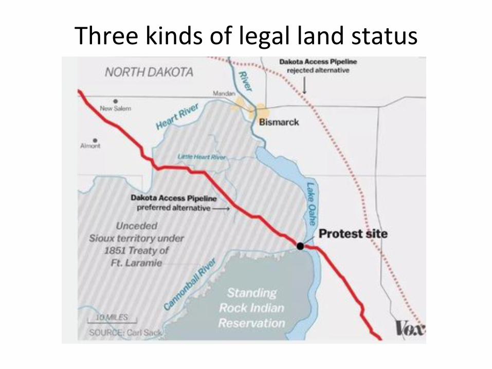
Threekindsoflegallandstatus

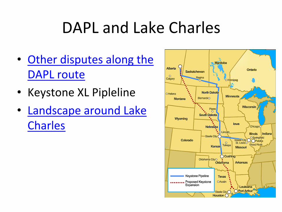
DAPLandLakeCharles

•  OtherdisputesalongtheDAPLroute

•  KeystoneXLPipleline•  LandscapearoundLakeCharles

Living standard

s

Energy Usage: 1750-2000

Coal

An Energy Dependent Society

Steam Steam locomotive

Power stations

Internal combustion engine

Air travel

Population growth

Global markets

1750 1800 1850 1900 1950 2000

Telecommunications

WWI WWII

Satellite

Environmental issues Micro-processor

Internet En

ergy

Usa

ge

?

Modifiers

Drivers

Cook and Sheath, 1997

Hydrocarbons Nuc

lear

Living Standards

Aseriesofreallycoolchartsonworldenergyhistory

Source:GailTvarberg,Ourfiniteworld.



RememberI=PAT?

Worldenergysupplies,1971-2014

6

Supply

Total pr imary energy supply by fuel

World

Other3

Natural gasOilBiofuels and waste

Coal2 NuclearHydro

0

2 000

4 000

6 000

8 000

10 000

12 000

14 000

1971 1975 1980 1985 1990 1995 2000 2005 2010 2014

World¹ total primary energy supply (TPES) from 1971 to 2014 by fuel (Mtoe)

1973 and 2014 fuel s hares of TPES

1. World includes international aviation and international marine bunkers. 2. In these graphs, peat and oil shale are aggregated with coal.

3. Includes geothermal, solar, wind, heat, etc.

6 101 Mtoe 13 699 Mtoe

Coal² 28.6%

Oil31.3%

Natural gas21.2%

Nuclear4.8%

Hydro2.4%

Biofuels and waste10.3%

Other³1.4%

Coal²24.5%

Oil46.2%

Natural gas16.0%

Nuclear0.9%

Hydro1.8%

Biofuels and waste10.5% Other³

0.1%

1973 2014

KEyWorld2016.indb 6 01/09/2016 11:38:34

Encapsula2ngEnvironmentalInjus2ce

Resiliencevariesdirectlywithproduc2vity

Resiliencevariesinverselywithproduc2vity

Intensifica2on

Produc2vityandEfficiency

QualitySustainabilityRe

silience

Nega2veExternality

PowerfulGroups

PowerlessGroups

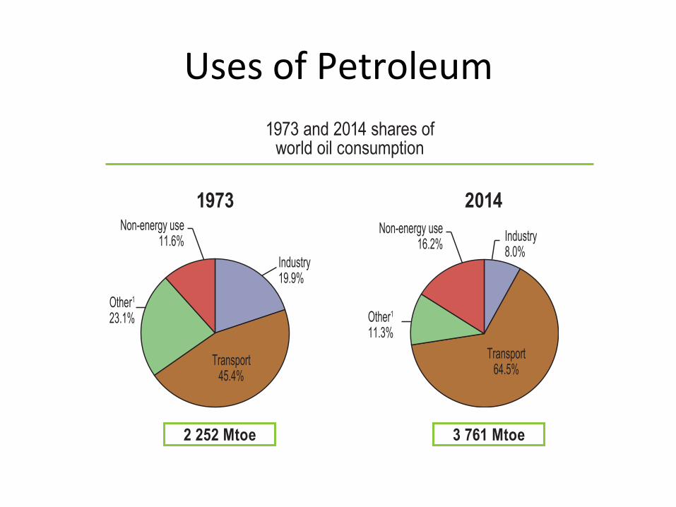
UsesofPetroleum

33

Consum p t i o n

Oil

Other1 TransportIndustry Non-energy use

0 500

1 0001 5002 0002 5003 0003 5004 000

1971 1975 1980 1985 1990 1995 2000 2005 2010 2014

Total final consumption from 1971 to 2014 by sector (Mtoe)

1973 and 2014 shares of world oil consumption

2 252 Mtoe 3 761 Mtoe1. Includes agriculture, commercial and public services, residential,

and non-specified other.

1973 2014

Industry19.9%

Transport45.4%

Other1

23.1%

Non-energy use11.6%

Non-energy use16.2% Industry

8.0%

Transport64.5%

Other1

11.3%

Total f inal consumption by sector

KEyWorld2016.indb 33 01/09/2016 11:38:42

SharesofAnthropogenicGHG

CO2 EMISSIONS FROM FUEL COMBUSTION Highlights (2015 Edition) - 7

INTERNATIONAL ENERGY AGENCY

1. KEY TRENDS IN CO2 EMISSIONSFROM FUEL COMBUSTION

The growing importance of energy-related emissions

Climate scientists have observed that carbon dioxide (CO2) concentrations in the atmosphere have been increasing significantly over the past century, com-pared to the pre-industrial era (about 280 parts per million, or ppm). The 2014 concentration of CO2 (397 ppm)3 was about 40% higher than in the mid-1800s, with an average growth of 2 ppm/year in the last ten years. Significant increases have also occurred in levels of methane (CH4) and nitrous oxide (N2O).

Energy use and greenhouse gases The Fifth Assessment Report from the Intergovern-mental Panel on Climate Change (Working Group I) states that human influence on the climate system is clear (IPCC, 2013). Among the many human activities that produce greenhouse gases, the use of energy rep-resents by far the largest source of emissions. Smaller shares correspond to agriculture, producing mainly CH4 and N2O from domestic livestock and rice culti-vation, and to industrial processes not related to energy, producing mainly fluorinated gases and N2O (Figure 1).

Within the energy sector4, CO2 resulting from the oxi-dation of carbon in fuels during combustion domi-nates total GHG emissions.

3. Globally averaged marine surface annual mean expressed as a molefraction in dry air. Ed Dlugokencky and Pieter Tans, NOAA/ESRL(www.esrl.noaa.gov/gmd/ccgg/trends/).4. The energy sector includes emissions from “fuel combustion” (thelarge majority) and “fugitive emissions”, which are intentional or un-

Figure 1. Shares of global anthropogenic GHG, 2010

* Others include large-scale biomass burning, post-burn decay,peat decay, indirect N2O emissions from non-agriculturalemissions of NOx and NH3, Waste, and Solvent Use.

Source: IEA estimates for CO2 from fuel combustion and EDGAR 4.3.0/4.2 FT2010 for all other sources.

Key point: Energy emissions, mostly CO2, account for the largest share of global GHG emissions.

CO2 emissions from energy represent over three quar-ters of the anthropogenic GHG emissions for Annex I5 countries, and about 60% of global emissions. This

intentional releases of gases resulting from production, processes, trans-mission, storage and use of fuels (e.g. CH4 emissions from coal mining). 5. The Annex I Parties* to the 1992 UN Framework Convention onClimate Change (UNFCCC) are: Australia, Austria, Belarus, Belgium,Bulgaria, Canada, Croatia, Cyprus*, the Czech Republic, Denmark,Estonia, European Economic Community, Finland, France, Germany,Greece, Hungary, Iceland, Ireland, Italy, Japan, Latvia, Liechtenstein,Lithuania, Luxembourg, Malta, Monaco, the Netherlands, New Zealand,Norway, Poland, Portugal, Romania, Russian Federation, theSlovak Republic, Slovenia, Spain, Sweden, Switzerland, Turkey,Ukraine, United Kingdom and United States. See www.unfccc.int.*For country coverage and geographical definitions please refer toChapter 5: Geographical Coverage.

Industrial processes 7%

Agriculture 11%

Others* 14%

90%

9%1%

CH4N2O

CO2 Energy 68%

HowDoWeKnowTheClimateisChanging?

•  Explana2ons:–  TheGreenhouseEffect–  SolarVaria2on–  Aerosols–  Albedochanges

Soucrce:NewYorkStateDepartmentofEnvironmentalConserva2on

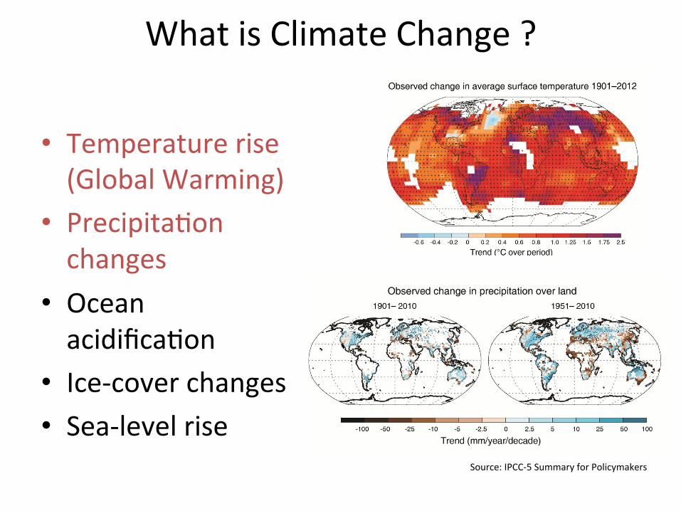
WhatisClimateChange?

•  Temperaturerise(GlobalWarming)

•  Precipita2onchanges

•  Oceanacidifica2on

•  Ice-coverchanges•  Sea-levelrise

Twelfth Session of Working Group I Approved Summary for Policymakers

IPCC WGI AR5 SPM-27 27 September 2013

Figure SPM.1 [FIGURE SUBJECT TO FINAL COPYEDIT]




Source:IPCC-5SummaryforPolicymakers

•  Temperaturerise(GlobalWarming)

•  Precipita2onchanges

•  Oceanacidifica2on

•  Ice-coverchanges•  Sea-levelrise







Key Points-

ide levels have risen in response to increased carbon dioxide in the atmosphere, leading to an increase in acidity (that is, a decrease in pH) (see Figure 1).

lower aragonite saturation levels (less availability of minerals) in the oceans around the world (see Figure 2).

2). However, decreases in cold areas may be of greater concern because colder waters typi-cally have lower aragonite levels to begin with.19

BackgroundThe ocean plays an important role in regulating the amount of carbon diox-ide in the atmosphere. As atmospheric concentrations of carbon dioxide rise (see the Atmospheric Concentrations of Greenhouse Gases indicator on p. 16), the ocean absorbs more carbon dioxide. Because of the slow mixing time between surface waters and deeper waters, it can take hundreds to thousands of years to establish this balance. Over the past 250 years, oceans have absorbed approxi-mately 40 percent of the carbon dioxide produced by human activities.17

Although the ocean’s ability to take up carbon dioxide prevents atmospheric levels from climbing even higher, rising levels of carbon dioxide dissolved in the ocean can have a negative effect on marine life. Carbon dioxide reacts with sea water to produce carbonic acid. The resulting increase in acid-ity (measured by lower pH values) reduces the availability of minerals such as aragonite, which is a form of calcium carbonate that corals, some types of plankton, and other creatures rely on to produce their hard skel-etons and shells. Declining pH and reduced availability of minerals can make it more difficult for these animals to thrive. This can lead to broader changes in the overall structure of ocean and coastal ecosystems, and can ultimately affect fish populations and the people who depend on them.18

While changes in ocean pH and mineral availability caused by the uptake of atmo-spheric carbon dioxide generally occur over many decades, these properties can fluctuate over shorter periods, especially in coastal and surface waters. For example, increased photosynthesis and respiration during the day and during the summer leads to natural fluctuations in pH. Acidity also varies with water temperature.

About the IndicatorThis indicator describes trends in pH and related properties of ocean water, based on a combination of direct observations, calculations, and modeling.

Figure 1 shows pH values and levels of dis-solved carbon dioxide at three locations that have collected measurements consistently over the last few decades. These data have been either measured directly or calculated from related measurements such as dissolved

Figure 1. Ocean Carbon Dioxide Levels and Acidity, 1983–2011This f igure shows the relationship between changes in ocean carbon dioxide levels (measured in the left column as a partial pressure—a common way of measuring the amount of a gas) and acidity (measured as pH in the right column). The data come from two observation stations in the North Atlantic Ocean (Canary Islands and Bermuda) and one in the Pacif ic (Hawaii). The up-and-down pattern shows the influence of seasonal variations.

250

300

350

400

450

500

1980 1990 1995 2000 2005 20101985 2015

Year

Diss

olve

d ca

rbon

dio

xide

(par

tial p

ress

ure

in m

icro

-atm

osph

eres

)7.95

8.00

8.05

8.10

8.15

8.20

1980 1990 1995 2000 2005 20101985 2015

pH [l

ower

pH

= m

ore

acid

ic]

250

300

350

400

450

500

1980 1990 1995 2000 2005 20101985 20157.95

8.00

8.05

8.10

8.15

8.20

1980 1990 1995 2000 2005 20101985 2015

250

300

350

400

450

500

1980 1990 1995 2000 2005 20101985 20157.95

8.00

8.05

8.10

8.15

8.20

1980 1990 1995 2000 2005 20101985 2015

Hawaii

Bermuda

Hawaii

Bermuda

Canary Islands Canary Islands

Data sources: Bates et al., 2012;20 González-Dávila, 2012;21 University of Hawaii, 201222

(Continued on page 45)

Ocean AcidityThis indicator shows changes in the chemistry of the ocean, which relate to the amount of carbon dissolved in the water.

44

WhatisClimateChange?

Sources:Top:EnvironmentalProtec2onAdministra2onMiddleandBofom:PCC-5SummaryforPolicymakers

pH


•  Empiricalevidence:Howgoodisit?– Temperature:virtuallycertain– Precipita2on:mediumconfidence– Oceanacidifica2onhighconfidence– Decreasingiceverylikely(Greenland)tolikely(Antarc2ca)

– Sea-levelverylikely

IPCC5thAssessmentReportSummaryforPolicymakers

WhatdoWeExpectWorldwide?

•  Valuesandrangesofuncertainty–  Temperaturerise(GlobalWarming)

–  Precipita2onchanges–  Oceanacidifica2on–  Ice-coverchanges–  Sea-levelrise







0.0=Currenttemperature

WhatdoWeExpectWorldwide?•  Valuesandrangesof

uncertainty–  Temperaturerise(Global

Warming)–  Precipita2onchanges–  Oceanacidifica2on–  Sea-levelrise–  Ice-coverchanges











•  Scienceandprobability•  Uncertainty•  Themisunderstandingofuncertainty•  Themanipula2onofuncertainty

Whodeniesclimatechangeandwhy

•  Atfirst:skep2calscien2sts(wantedevidence)•  Corpora2onswhowillbenefitfromcon2nuedstatusquo

•  Peoplewithaninnatesenseofdistrust(seeins2tu2onschaptersofStrangers)

•  Poli2cianswho– BenefitfromContribu2ons– Needvotesfrompeoplewhodistrustins2tu2ons

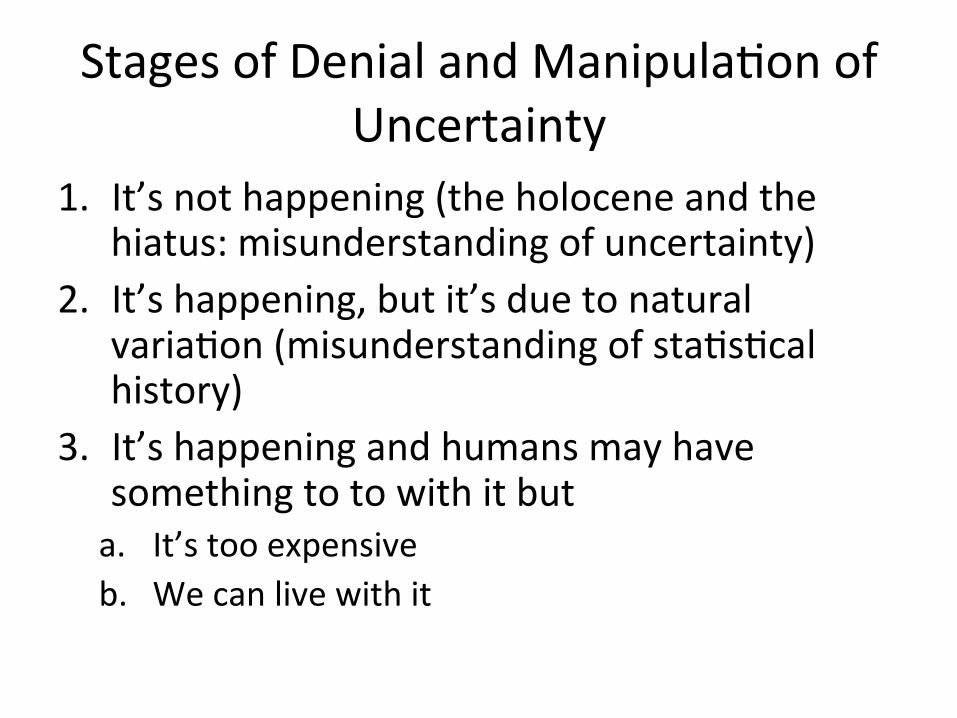
StagesofDenialandManipula2onofUncertainty

1.  It’snothappening(theholoceneandthehiatus:misunderstandingofuncertainty)

2.  It’shappening,butit’sduetonaturalvaria2on(misunderstandingofsta2s2calhistory)

3.  It’shappeningandhumansmayhavesomethingtotowithitbuta.  It’stooexpensiveb.  Wecanlivewithit


1.  It’snothappening(theholoceneandthehiatus:inten2onalmisunderstandingofuncertainty)

CO2levelsaretoday,amongthelowestinthepast600millionyears.CO2levelswerehigherthantodayin85%ofthepast600millionyears.CO2levelswereasmuchas202meshigherinthegeologicalpast.CO2levelswereatleast52meshigherthantodayinthedinosaurperiod.TherewerethreeiceageswithmoreCO2thantoday,onehadfileen2mesmore.CO2hasneverbeenobservedinthegeologicalrecordtobeadriveroftheclimate,evenwhenlevelsweresignificantlyhigherthantoday.CO2,byitself,cannotcausemuchwarming.Fortheretobedangerouswarming,otherthingsmustoccur,whichwouldacceleratethewarming,calledposi2vefeedbacks.Themostlikelyisincreasedatmosphericwatervapor.Posi2vefeedbackshavenotbeenobservedtoexistinthepastandwhenCO2levelsweresignficiantlyhigherthantoday.Atmospherichumidityisalsoactuallyindecline.linkGlobaltemperaturesweremostlywarmerthantodayintheprior8,000years,theHolocene.link

WhatBreitbarthastosay




NATURE CLIMATE CHANGE | VOL 6 | MARCH 2016 | www.nature.com/natureclimatechange 225

opinion & comment

global surface warming. For example, new research has shown that decadal timescale cooling of tropical Pacific sea surface temperature (SST) — which is linked to trade-wind intensification associated with the negative phase of the Interdecadal Pacific Oscillation (IPO) — made a substantial contribution to the warming slowdown11–14 (Fig. 2e). Since averaging over a large number of climate model simulations reduces the random noise of internal variability, and assuming a large contribution from internal variability in the slowdown, the mean of the multi-model ensemble (MME) could not be expected to reproduce the slowdown.

A different perspective on the role of internal variability is obtained through the analysis of the individual models and realizations comprising the MME. In 10 out of 262 ensemble members, the simulations and observations had the same negative phase of the IPO during the slowdown period — that is, there was a fortuitous ‘lining up’ of internal decadal variability in the observed climate system and the 10 simulations15,16. These 10 ensemble members captured the muted early-twenty-first-century warming, thus illustrating the role of internal variability in the slowdown.

Related work has identified additional contributions to the slowdown from decadal variability arising in the Indian17 and Atlantic Oceans18. However, the flow of heat in these and other ocean basins (including the tropical Pacific) remains poorly constrained by measurements. Other positive outcomes of this slowdown research include better understanding of the influence of uncertainty in ocean SSTs on decadal timescale GMST trends4, and of the role of decadal changes in volcanic forcing in partially offsetting human-caused warming19. Research has also identified a systematic mismatch during the slowdown between observed volcanic forcing and that used in climate models19.

It has been suggested20 that the lack of Arctic surface measurements has resulted in an underestimate of the true rate of GMST increase in the early twenty-first century. Independent satellite-based observations21,22 of the temperature of the lower troposphere (TLT; Fig. 2f) have near-global, time-invariant coverage. Although satellite TLT datasets also have important uncertainties21, they corroborate the slowdown of GMST increase23 and provide independent evidence that the slowdown is a real phenomenon.

These examples have built upon earlier advances in our scientific understanding of the causes of fluctuations in GMST. For example, the cooling after the Pinatubo

eruption in 1991 was predicted before it could be observed. The ability of climate models to simulate this cooling signal was reported in published papers and IPCC assessments. Previous work noted the importance of the ‘spring-back’ from Pinatubo, which contributed to relatively rapid rates of global warming over the decade of the 1990s (for example, ref. 23); a similar spring-back occurred in the 1980s after El Chichón.

Understanding of the recent slowdown also built upon prior research into the causes of the so-called big hiatus from the 1950s to the 1970s. During this period, increased cooling from anthropogenic sulfate aerosols roughly offset the warming from increasing GHGs (which were markedly lower than today). This offsetting contributed to an approximately constant GMST. Ice-core sulfate data from Greenland support this interpretation of GMST behaviour in the 1950s to 1970s, and provide compelling evidence of large temporal increases in atmospheric loadings of anthropogenic sulfate aerosols. The IPO was another contributory factor to the big hiatus13.

Research motivated by the warming slowdown has also led to a fuller understanding of ocean heat uptake17,24 in the context of decadal timescale variability in GMST. Improved understanding was only possible after recent progress in identifying and accounting for errors in observed estimates of ocean heat content (OHC)25, and by advances in isolating the signatures

of different modes of variability in OHC changes. In summary, research into the causes of the slowdown has been enabled by a large body of prior research, and represents an important and continuing scientific effort to quantify the climate signals associated with internal decadal variability, natural external forcing and anthropogenic factors.

Claims and counterclaimsRecent claims by Lewandowsky et al. that scientists “turned a routine fluctuation into a problem for science” and that “there is no evidence that identifies the recent period as unique or particularly unusual”26 were made in the context of an examiniation of whether warming has ceased, stopped or paused. We do not believe that warming has ceased, but we consider the slowdown to be a recent and visible example of a basic science question that has been studied for at least twenty years: what are the signatures of (and the interactions between) internal decadal variability and the responses to external forcings, such as increasing GHGs or aerosols from volcanic eruptions?

The last notable decadal slowdown during the modern era occurred during the big hiatus. The recent decadal slowdown, on the other hand, is unique in having occurred during a time of strongly increasing anthropogenic radiative forcing of the climate system. This raises interesting science questions: are we living in a world less sensitive to GHG forcing

1950 1960 1970 1980 1990 2000 2010

Year

−0.4

−0.2

0.0

0.2

0.4

0.6

0.8

GM

ST a

nom

aly

(°C)

Big hiatus Warming slowdown

El C

hich

ón

Pina

tubo

HadCRUT4.4NOAA-KarlGISTEMPCMIP-5

Figure 1 | Annual mean and global mean surface temperature anomalies. Anomalies are from three updated observational datasets3–5 and the ensemble mean (black curve) and 10–90% range (darker grey shading) GMST of 124 simulations from 41 CMIP-5 models using RCP4.5 extensions from 200528. Anomalies are relative to 1961–1990 climatology. We obtain 1972 as the end year of the big hiatus (the period of near-zero trend in the mid-twentieth century) by constructing an optimal piece-wise bilinear fit to the NOAA-Karl data over the period 1950 to 2001. We hence use 1972–2001 as a baseline period, a period similar to the WMO climate normal period 1971–2000, against which the early-twenty-first-century records can be compared. Using the 1971–2000 period rather than the baseline determined by a bilinear fit to the data (yielding a 1972 start date) does not materially change the result. Choice of the 2001 start year of the warming slowdown avoids possible end-point effects associated with large El Niño or La Niña events in 1998 and 2000 (respectively).

© 2016 Macmillan Publishers Limited. All rights reserved

Fyfeetal.,NatureClimateChange,2016




3.  It’shappeningandhumansmayhavesomethingtotowithitbuta.  It’stooexpensiveb.  Wecanlivewithit

HowDoWeDecideWhattoDo?

•  UncertaintyandPrecau2on•  UncertaintyandDiscoun2ng•  UncertaintyandManipula2on

petroleum, energy, injus2ce, and science denial

Documents