Phasor Measurement Unit Datain Power System State Estimation

Intermediate Project Report

Power Systems Engineering Research Center

A National Science FoundationIndustry/University Cooperative Research Center

since 1996

PSERC

Power Systems Engineering Research Center

Phasor Measurement Unit Data in Power System State Estimation

Intermediate Project Report for the PSERC Project

“Enhanced State Estimators”

Report Authors

Mark Rice Gerald T. Heydt

Arizona State University

PSERC Publication 05-02

January 2005

Information about this project For information about this project contact: Gerald T. Heydt, Ph.D. Arizona State University Department of Electrical Engineering Tempe, AZ 85287 Tel: 480-965-8307 Fax: 480-965-0745 Email: heydt@asu.edu Power Systems Engineering Research Center This is a project report from the Power Systems Engineering Research Center (PSERC). PSERC is a multi-university Center conducting research on challenges facing a restructuring electric power industry and educating the next generation of power engineers. More information about PSERC can be found at the Center’s website: http://www.pserc.org. For additional information, contact: Power Systems Engineering Research Center Cornell University 428 Phillips Hall Ithaca, New York 14853 Phone: 607-255-5601 Fax: 607-255-8871 Notice Concerning Copyright Material PSERC members are given permission to copy without fee all or part of this publication for internal use if appropriate attribution is given to this document as the source material. This report is available for downloading from the PSERC website.

©2004 Arizona State University. All rights reserved.

Acknowledgements

The Power Systems Engineering Research Center sponsored the research project titled “Enhanced State Estimators.” The project began 2004 and is expected to be completed in 2005. This report is an intermediate report of progress at Arizona State University.

We express our appreciation for the support provided by PSERC’s industrial members and by the National Science Foundation under grant NSF EEC-0001880 received under the Industry / University Cooperative Research Center program.

The authors thank all PSERC members for their technical advice on the project, especially Dale Krummen (AEP), Jay Giri (AREVA T&D), Jerome Ryckbosch (RTE), and Ram Adapa (EPRI) who are industry advisors for the project. The authors also acknowledge Drs. Ali Abur and A. P. Sakis Meliopoulos of Texas A&M University and Georgia Tech respectively who contributed technical advice and data to this work. Dr. Abur is the project leader.

i

Executive Summary

This report deals with the placement of phasor measurement units (PMUs) based on the improvement in error in the estimate of the voltage phase angles in power systems. The present technology measures voltage, current, and real and reactive power for determining the operating condition of the electric network. This technology cannot measure voltage phase angle directly. Thus, voltage phase angles must be found by state estimation.

This research examined two possible methods for incorporating phasor measurement units into present state estimation methods. The two principal state estimation methods considered are: 1) using weighted least squares with significant weight on the PMU measurements; and 2) eliminating the equations associated with the voltage phase angle measurements made by the PMU. The PMU measurements would be done using global positioning system (GPS) technology to measure voltage phase angles; this measurement would be very accurate.

The test bed for the state estimation methodology assessment is the Institute Electrical and Electronics Engineering (IEEE) 14 bus system. In this study, the IEEE 14 bus system is fully observable by supervisory control and data acquisition (SCADA) devices. The incorporation of PMU measurements into the system increases the accuracy of the voltage phase angle estimates. The cases considered examine the location of the PMUs based on decreasing the error in the estimate of voltage phase angle. The work includes an examination of the impact of noise on the location of the PMUs. Also included in this work is the relationship between the number of PMUs installed and the error in the voltage phase angle estimates. A goal of this work is to show the gains that can be attained by PMUs.

ii

Table of Contents

1. State Estimation: Past, Present, and Future ................................................................ 1

1.1 Background and Motivation ................................................................................... 1

1.2 State Estimation Literature Review ........................................................................ 1

1.3 The Pseudoinverse and Its Relationship to Least-Squares Estimation ................... 2

1.4 Phasor Measurement Units Literature Review ....................................................... 2

1.5 Organization of the Report ..................................................................................... 3

2. The Basis of Linear State Estimation.......................................................................... 5

2.1 The Method of Least Squares ................................................................................. 5

2.2 Weighted Least Squares.......................................................................................... 5

2.3 Norms...................................................................................................................... 7

2.4 Condition Numbers................................................................................................. 8

3. Experiments Utilizing PMU Measurements in State Estimators................................ 9

3.1 Adding PMU Measurements to a State Estimator .................................................. 9

3.2 Problem Statement .................................................................................................. 9

3.3 Solution by Weighted Least Squares Estimation.................................................... 9

3.4 Solution by Direct Substitution............................................................................. 11

3.5 Metrics for Comparing WLS to Direct Substitution............................................. 11

3.6 Design of the Experiments.................................................................................... 13

3.7 Description of the Code ........................................................................................ 14

3.8 Results from the MATLAB .................................................................................. 15

3.9 Noise Dependency ................................................................................................ 17

3.10 Conclusions........................................................................................................... 19

4. Experiments Utilizing Multiple PMU Measurements in State Estimators ............... 20

4.1 Adding PMU Measurements to a State Estimator ................................................ 20

4.2 Description of the MATLAB Script ..................................................................... 20

4.3 Results from Direct Substitution of Two PMU Measurements............................ 20

4.4 Results from Weighted Least Squares Method of Two PMU Measurements...... 21

4.5 Effect of Noise on Placement of PMUs................................................................ 21

4.6 Additional of PMU Measurements ....................................................................... 26

4.7 Examination of the Variance of the E-vector ....................................................... 27

iii

Table of Contents (continued)

4.8 Conclusions........................................................................................................... 30

5. Conclusions and Future Work .................................................................................. 31

5.1 Conclusions........................................................................................................... 31

5.2 Future Work.......................................................................................................... 32

REFERENCES ................................................................................................................. 33

A. IEEE14 Bus Test Bed System Information .............................................................. 35

B. MATLAB Scripts for State Estimation..................................................................... 38

B.1 Script for a Single PMU in the 14 Bus System..................................................... 38

B.2 Script for Examining Two PMU in the 14 Bus System........................................ 45

B.3 Script to Examine Impact of Multiple PMUs on the 14 Bus System ................... 53

C. Summary of Experiments Performed........................................................................ 61

iv

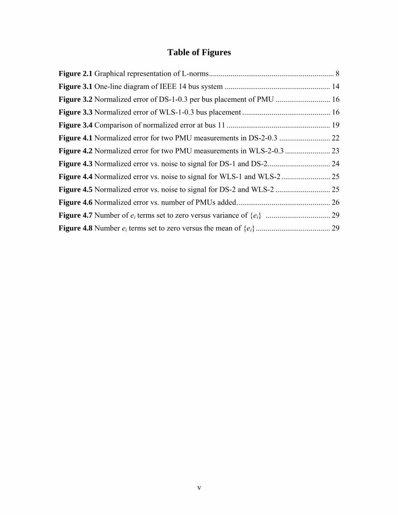
Table of Figures

Figure 2.1 Graphical representation of L-norms................................................................ 8

Figure 3.1 One-line diagram of IEEE 14 bus system ...................................................... 14

Figure 3.2 Normalized error of DS-1-0.3 per bus placement of PMU ............................ 16

Figure 3.3 Normalized error of WLS-1-0.3 bus placement ............................................. 16

Figure 3.4 Comparison of normalized error at bus 11 ..................................................... 19

Figure 4.1 Normalized error for two PMU measurements in DS-2-0.3 .......................... 22

Figure 4.2 Normalized error for two PMU measurements in WLS-2-0.3 ....................... 23

Figure 4.3 Normalized error vs. noise to signal for DS-1 and DS-2................................ 24

Figure 4.4 Normalized error vs. noise to signal for WLS-1 and WLS-2......................... 25

Figure 4.5 Normalized error vs. noise to signal for DS-2 and WLS-2 ............................ 25

Figure 4.6 Normalized error vs. number of PMUs added................................................ 26

Figure 4.7 Number of ei terms set to zero versus variance of {ei} ................................. 29

Figure 4.8 Number ei terms set to zero versus the mean of {ei}...................................... 29

v

Table of Tables

Table 3.1 List of various measurements of error in the state vector .................................13

Table 3.2 Normalized error of as PMU location is varied............................................17 δ̂

Table 3.3 Normalized error as bus placement and noise level varied for DS-1................18

Table 3.4 Normalized error as bus placement and noise level varied for WLS-1 ............18

Table 4.1 Placement of two PMUs at varying signal to noise ratio in WLS-2 .................24

Table A.1 Solved delta values for IEEE 14 bus system....................................................35

Table A.2 Line impedances and power flow for 14 bus system .......................................36

Table A.3 H matrix for the 14 bus test system..................................................................37

Table C.1 Experiments performed ....................................................................................62

vi

1. State Estimation: Past, Present, and Future

1.1 Background and Motivation The electric power industry is undergoing multiple changes and restructuring towards deregulation. As the restructuring is happening profits are less guaranteed, and some electric power utilities are increasing the loads on the grid to generate more revenue. The increased power exchange has a concomitant requirement for situational awareness. This refers to the need for system operators to know the operating states of the system.

The Northeast blackout of 2003 was in part caused by the national electric grid being pushed past is limits and the operators not detecting that the grid was in a critical state [1]. If the operators of the electric grid in Ohio had been able to detect that several areas the grid were in critical states, they might have been able to prevent the cascading events which followed. One key element of modern energy management systems is a state estimator: a state estimator uses system inputs and a system model to obtain and depict the power system states (mainly bus voltage magnitudes and phase angles).

Most utilities have state estimators in the package of energy management systems. Due to the fact that state estimators tend to not accurately represent the system during times of use of incorrect measurements (a condition which is flagged by the estimator), the system operators might turn off this function, have low confidence in the displayed values, or ignore displays. There are several topics in state estimation being studied to improve the accuracy of the state estimation in power systems. In this report the author examines how new technology of a phasor measurement units, a global positioning system (GPS) technology can be used to help better the estimation of the states in an electrical power systems.

1.2 State Estimation Literature Review Schweppe was one of the first to formulate static state estimation for a power network based on the power flow model [2]. The idea is to estimate the states of the power network. These states might not be directly observable based on physical relationships between the measurements and the desired unknown states. The model developed by Schweppe requires that the physical state of the system is known, e.g. breaker status [2].

Another advancement in the field of state estimation was the introduction of a weight matrix to increase the accuracy of the results. Weighting is done to enhance the “input” of accurate measurements, and de-emphasize the less accurate measurements. It can be shown that the maximum likelihood estimate utilizes weights that are based on the covariance of the measurement devices. The more accurate a measurement, the more weight in the state estimator [3]. Weighting is the practice of accounting for the confidence in a measurement. The process of overcoming measurement noise is inherent in taking physical measurements, but there are situations in which the data are grossly erroneous. The data that are erroneous must be identified and eliminated. One method for the detection of bad data is the examination of the measurements and if the measurements deviate from expected values by some preset threshold the measurement

1

can be assumed to be bad [4]. Another problem that causes state estimators inaccuracies is the model itself. Generally the simple linear model Hx=z is used where the H is the measurement model (processing matrix), x is the state vector, and x is the measurements. If the process matrix is incorrect, the model does not represent what is physically happening in the system. The detection of both erroneous data or improper formation of the process matrix may be done by examining the residual of the equation Hx=z [3]. The common technique in correcting the issue of unobservable areas is to provide an estimate of what the readings are in the unobservable areas to create an entire system model [5].

References [6, 7, 8, 9] are textbooks on state estimation in power engineering; references [10 -- 14] are representative of solutions methods; and [4, 15] are case studies.

1.3 The Pseudoinverse and Its Relationship to Least-Squares Estimation The commonly used model for a linear system is

Hx=z (1.1)

with H as the process matrix (m by s matrix), x is the state vector (dimension s), and z is the measurement vector (dimension m) is overdetermined when m is larger than s. References [6 – 9, 16] describe Equation (1.1). Equation (1.1) can be “solved” in the least-square sense by minimizing ||r||2,

r=Hx-z (1.2)

where || ● ||2 refers to the 2-norm [8]. Properties of norms appear in [8]. It can be shown that || r ||2 is minimized when

. (1.3) zHxx +== ˆ

The notation is the “estimate” of vector x, H+ pseudoinverse of H. References [6 – 9, 16] describe the properties of the pseudoinverse. Equation (1.3) is known as an unbiased least squares estimator.

x̂

1.4 Phasor Measurement Units Literature Review Phasor measurement units (PMUs) are instruments that take measurements of voltages and currents and time-stamp these measurements with high precision. PMUs are equipped with Global Positioning Systems (GPS) receivers. The GPS receivers allow for the synchronization of the several readings taken at distant points [17]. PMUs were developed from the invention of the symmetrical component distance relay (SCDR). The SCDR development outcome was a recursive algorithm for calculating symmetrical components of voltage and current [18]. Synchronization is made possible with the advent of the GPS satellite system. The GPS system [19] is a system of 36 satellites (of which 24 are used at one time) to produce time signals at the earth’s surface. GPS receivers can resolve these signals into {x,y,z,t} coordinates. The t coordinate is time. This is accomplished by solving the distance=(rate)(time) in three dimensions using satellite signals. The PMU records the sequence currents and voltages and time stamps

2

the reading with time obtained by the GPS receiver. It is possible to achieve accuracy of synchronization of 1 microsecond or 0.021° for 60 hertz signal. This is well in the suitable range of measuring power frequency voltages and currents [18]. Based upon the research done at Virginia Tech, the Macrodyne Company was able to begin production of PMU devices, which has lead to the IEEE Standard 1344 “Sychrophasor” which defines the output data format of a PMU [18].

PMUs are able to measure what was once immeasurable, phase difference at different substations. When completing a state estimation of a power system one of the states, which are being determined, is the voltage angle at each bus. With PMUs the utilities are able to directly measure voltage angle as compared to the swing bus.

Since the development of the PMU, power engineers have been looking at how to use the device to better observe the system. The PMUs have been implemented as a source of information to detect faults on transmission lines [19]. The implementation of PMUs to make the system more observable starts with a spanning tree and looks for areas of the system which are unobservable. The next step is to impose certain criteria on the search of the proper placement of the PMUs. Three that have been looked at are modified simulated annealing method, direct combination, and tabu search. All three where examined on tests on the IEEE 14, 30, and 57 bus systems and the results show that the proposed methods can find the optimal solution in an efficient manner [17]. The other method for determining the optimal placement of the PMU is to do a genetic algorithm search, the authors suggest that a genetic search is the best because the two solution criteria may be in opposition of each other. In this case, criterion one is to maximize the redundancy and observable area of system. Criterion two is to minimize cost of the installation [20]. Another paper argues there should be more criteria added to the optimal placement of PMU including the examination of placement of the devices with consideration given to improving the security of the system [21].

How PMUs should work in state estimation has been discussed. There is a school of thought that the measurements from the PMU are far superior of SCADA data used in traditional state estimation and should be collected and used separate from this data [21]. Others admit there is difference in the information and it is viable to use PMU measurements in with SCADA data [22]. Hydro-Quebec believes that the PMUs are accurate enough to not need correlation between PMS measurements. Their algorithm is to place the PMUs based on the busses which minimize the correlation between measurements [23].

1.5 Organization of the Report The report is organized into five chapters. Chapter one examines the work that has already been done in the field of state estimation and phasor measurement units. Chapter two examines the theory behind state estimators. In chapter two, there is an examination of the different types of the state estimators including least squares. In Chapter two there is an examination of alternative norms. Chapter three addresses the question of PMU placement. That is, to identify the bus phase angle for which the perfect knowledge would produce the best improvement in estimator accuracy. Chapter four contains experiments with multiple PMUs in the IEEE 14 bus system. Chapter five contains

3

conclusions about the method studied in this report and future work to make the method more refined and applicable for real world systems.

Three appendices are attached to the report:

A. A description of a 14 bus test bed system B. MATLAB scripts used in this work C. A listing of all experiments done and the conditions of these experiments.

4

2. The Basis of Linear State Estimation

2.1 The Method of Least Squares Present state estimation techniques rely on the least squares approach to finding the best estimation of states. The method of least squares uses the linear equation,

zHx = (2.1)

H is the process matrix dimensioned (m x s), x is the state vector dimensioned (s), and z is the measurement vector dimensioned (m). In state estimation it assumed that the system is over determined, meaning there are more measurements than states. However rarely are the measurements perfect, and therefore z is actually a perfect measurement plus ‘noise.’ The problem becomes how to find the best fit between measurements z and states x. In the least squares approach idea is minimize the difference L2

norm of the residual,

Hxzr −= (2.2)

( ) ( )t2 zHxzHxr −−=2|| . (2.3)

To minimize Equation 2.3, take the derivative, which results in Equation 2.4. Then simple algebra is used to separate the best estimate of x, namely , x̂

zHxHHxr tt

xx

−==∂

∂

=

ˆ0||

ˆ

22 (2.4)

zHxHH tt =ˆ ( ) zHHHx ttˆ =1− . (2.5)

The formulation in (2.5) is valid only when HtH is nonsingular. The singular case is rarely encountered but can be handled by an alternative formatting. There are two notable terms in Equation (2.5): (HtH)-1Ht term to this equation the pseudoinverse (2.7) and the gain matrix (2.6),

H (2.6) HG t=

( ) tt HHHH + =1− . (2.7)

The notation H+ refers to the pseudoinverse.

2.2 Weighted Least Squares

A drawback of the least squares approximation is that the all the measurements are treated with the same weight. This procedure is unbiased. This implies that all the

5

measuring tools are measuring with the same accuracy and precision. In power engineering, this is rarely the case. A term is added to the least squares to provide emphasis for accurate measurements. This is accomplished by weighting the residual r using a weighting matrix W. The matrix W is m by m, and the weighted residual is W(Hx-z). The W diagonal entries are the inverse of the covariance of the measurements in order to obtain the maximum likelihood solutions [7],

(2.8)

⎥⎥⎥⎥⎥⎥

⎦

⎤

⎢⎢⎢⎢⎢⎢

⎣

⎡

=

−

−

−

2

22

21

m

W

σ

σσ

ΟΟ

( )zHxWr −= (2.9)

( )[ ] ( )[ ]t2 zHxWzHxWr −−=2|||| . (2.10)

Equation 2.9 is the weighted residual equation. Moving the W inside the parenthesis it is found an equation similar to least squares. To find the x this minimizes ||r||22 take the derivative,

( ) ( )WzWHxWzWHxr t −−=22||||

Wzz =′WHH =′

( ) ( )t2 zxHzxHr ′−′′−′=2|||| (2.11)

zHxHHxr tt

xx

′′−′′==∂

∂

=

ˆ0||

ˆ

22

( ) zHHHx t ′′′′=ˆ −1 . (2.12)

A weakness of weighted least squares is that if a measurement is known to high precision, it is difficult to represent that in the W matrix. In the case below, assume that c is much greater than a and b,

⎥⎥⎥

⎦

⎤

⎢⎢⎢

⎣

⎡=

3231

2221

1211

10hhhhhh

H a

⎥⎥⎥

⎦

⎤

⎢⎢⎢

⎣

⎡

=c

b

b

ww

wW

100001000010

3

2

1

6

⎥⎦

⎤⎢⎣

⎡′′

=2221

1211

hhhh

WHH t ′′

acbaba +++′ 222

acbaba +++′′

acbaba +++′ 222

whwhwhh ++= 101010 33122111111

whhwhhwhhhh ++== 101010 3323122221112112112

. whwhwhh ++= 101010 33222211222

If c is much larger than b and a, any term raised to the c power is much larger than the rest. This causes the matrix HtWH to approach being singular. Depending on precision of the software package being used and the magnitude of the difference between c and a and b can cause the terms not raised to the c power to be dropped completely.

2.3 Norms

The state estimation technique presented relies on the L2 being a satisfactory in representing the error between the measurements and the states. The Lp norm is,

( )pm

i

pip xr ∑

=

=0

|||||| . (2.13)

There are several L norms however three most commonly discussed are the L1, L2, and the L∞ norm. The L1 norm is the sum of the absolute of the number as seen in Equation 2.14. The L2 norm is the square root of the sum of the squares, and the L∞ norm is the largest single value in the vector,

L1-Norm (2.14) ∑=

=m

iixr

11 ||||||

L2-Norm ( )∑=

=m

iixr

1

22|||| (2.15)

L∞-Norm ( ) ||max||||||1

i

m

ii xxr == ∞

=

∞∞ ∑ . (2.16)

A plot can be created of the different norms of a vector of dimension two,

x=(x1, x2)t (2.17)

. (2.18) ppp kx =||||

7

Figure 2.1 shows loci of ||x||p=k. L norms are a way of collapsing data stored in a vector into a single value.

- k k

k

x 1

x 2

|| x|| 2=k

|| x|| 1=k

- k

||x||∞=k

Figure 2.1 Graphical representations of L-norms

2.4 Condition Numbers State Estimation based on the Hx=z has a weakness that small perturbations in vector z or matrix H can cause large changes in the estimated state vector, . The condition number of a matrix is the largest singular value divided by the smallest singular value. The singular value matrix is a diagonal matrix determined by,

x̂

nmA ×ℜ∈ mmU ×ℜ∈ nnV ×ℜ∈

( )pdiagAVU ,...,, 21T σσσ= } { nmp ,min= (2.25)

( ) +⋅== AAAcond2

1

σσ . (2.26)

The condition number quantifies how close the matrix is to being orthogonal or singular. An orthogonal matrix has a condition number of 1 and singular matrix has a condition number of infinity. As the condition number approaches 1, or is small, the matrix is considered well conditioned. The counter statement is that as the condition number of a matrix is large, then the matrix is considered ill-conditioned or close to being a singular matrix. Though not a linear map the larger the condition number of a matrix the larger the amplification of a perturbations in either the z vector or H matrix will map to the estimated state vector, . x̂

8

3. Experiments Utilizing PMU Measurements in State Estimators

3.1 Adding PMU Measurements to a State Estimator PMUs are able to make highly accurate phase angle measurements compared to conventional measurements made by SCADA devices. Retrieving data from the PMUs to merge them with data from SCADA devices for state estimation can be problematic. Hyper accuracy of PMU data may not be warranted. PMUs are able to directly measure voltage angles [24]. As discussed previously, voltage phase angle is one of the states to be estimated. The addition of a voltage phase angle measurement to a conventional state estimator could greatly increase the accuracy of the state estimator if implemented correctly. The two options examined in this report are to add PMU measurement into the state estimator with significant weight on this new measurement; or to eliminate the equations that correspond to the measured states. These two philosophies are examined in this chapter.

3.2 Problem Statement The state estimator used in this research is based on DC load flow model. In the DC model, the P -- δ relationship is decoupled from the Q -- |V| relationship. Because the objective is to improve accuracy, only the P – δ decoupled equations are used. The basic equations are of the form,

δ̂

Hxz = .

In this expression, z is the measurement vector, H is the process matrix and x is the state vector. With added PMU measurements the equation becomes,

. (3.1) ⎥⎦

⎤⎢⎣

⎡⎥⎦

⎤⎢⎣

⎡=⎥

⎦

⎤⎢⎣

⎡ +

GPSGPS IHH

zz

δδη 121

0

Note that in (3.1), the measurements z are contaminated by noise η, and augmented by PMU measurements zGPS. The subscript ‘GPS’ refers to the ultimate source of angular measurements made by the PMU. Submatrices H1 and H2 are the original H matrix partitioned into the parts which correspond to the δ and δGPS. The I matrix is an identity matrix of suitable dimension. This paper examines two possible methods for dealing with the formulation in (3.1): weighted least squares estimation; and estimation after the direct substitution of zGPS into the remaining equations.

3.3 Solution by Weighted Least Squares Estimation

The standard weighted least squares implementation was described in chapter 2. The solution of (3.1) by weighted least squares estimation (e.g. Equation (2.12)) results in,

9

, ⎥⎦

⎤⎢⎣

⎡ +=′

gpszz

zη

, ⎥⎦

⎤⎢⎣

⎡=

IH

0' 21 HH

and

, ⎥⎦

⎤⎢⎣

⎡=′

−

−

2

21

00

GPS

Wσ

σ

where

. 221

−− << GPSσσ

The estimate of becomes ⎥⎦

⎤⎢⎣

⎡=

GPSδδ

δ 1

( ) zWHHWH tt ′′′′′′=−1δ̂ . (3.4)

In (3.4), the vector and matrices have dimension as follows,

s by 1 δ̂

H’ (m+g) by s

W’ (m+g) by (m+g)

z' (m+g) by 1

where s is the total number of states to be estimated (including the δGPS states); m is the dimension of measurements excluding the PMU measurements; g is the number of PMU phase angle measurements. Note that in the over determined case m+g > s. Experiments using the augmented weighted least squares method will be denoted by WLS.

A variation on this method of the state estimation is to replace the estimated values for the voltage phase angles associated with PMU measurements with the measurements made by the PMU, after the state estimation is completed. This will generally decrease the amount of error in the answer. WLSp denotes experiments using this method of replacing the voltage phase angle measurements after the estimation.

10

3.4 Solution by Direct Substitution An alternative approach offered in this report is concept of direct substitution. The approach denominated “direct substitution” is offered as an alternative to the direct implementation of weighted least squares estimation described in section 3.3. DS denotes experiments using direct substitution. Again starting with Equation (3.1), multiplying out the right hand side of the equation yields

GPSHHz δδη 211 +=+

and GPSGPSz δ= .

Substitute the PMU measurements for the voltage phase angles,

112 δη HzHz GPS =−+ .

The state estimation equation for direct substitutions is

( )GPSzHzH 211̂ −+= + ηδ . (3.5)

In (3.5), the vectors and matrices have dimensions as follows

(s-g) by 1 H1 m by (s -- g) δ̂

H1+ (s -- g) by m z m by 1

η m by 1 H2 m by g

zGPS g by 1.

3.5 Metrics for Comparing WLS to Direct Substitution The residual vector is typically used to determine the fit of the measurements to the model in power system state estimation. The residual is used because when state estimation is being conducted for an actual system, the ‘true’ values of the states are not known. The residual vector as discussed earlier is xHzr ˆ−= . It is convenient to use the 2-norm of the r as an index of the agreement of the measurement equations,

22

rrr t=

xHzr ˆ−=

11

For comparing weighted least squares to direct substitution there are several reasons why

the residual may be inappropriate. The first reason is that the z and vectors are of

two different dimensions. The second reason is that the introduction of weights into the Hx=z expression causes a weighted residual to be not comparable to the unweighted counterpart.

⎥⎦

⎤⎢⎣

⎡

GPSzz

In this study the IEEE 14 bus system is used [25]. A benefit of using a widely publicized test system is the exact solution is known and solution techniques among researchers may be compared. In this study, it is possible to examine the deviation of from the “exact” value of x. Normally this comparison is not possible but because of the use of a test bed with a known solution, it is possible to use normalized error, N.E., to assess the accuaracy of ,

x̂

x̂

2

2ˆ

exact

exact

xxx

NE−

= . (3.6)

The normalized error has benefits for comparing direct substitution to weighted least squares. The normalization permits comparison of residual norms for residual vectors of different dimensions. Table 3.1 shows the various measurements of error.

12

Table 3.1 List of various measurements of error in the state vector

Normalized Error 2

2ˆ

exact

exact

xxx

NE−

=

Norm of the Residual 22x̂Hzr −=

Weighted Residual Norm 22

x̂HWzWrw −=

RMS of Residual 2ˆ1 xHz

mRrms −=

3.6 Design of the Experiments

In this section, two experiments are offered to illustrate the differences between direct substitution and weighted least squares method. Appendix C lists all the experiments. The focus will be minimizing the normalized error and effects of different noise to signal levels.

The IEEE 14 bus system depicted in Figure 3.1 consists of 14 buses, 3 have generators and the other 11 are considered load buses. The system also has 3 transformers. The base case is known, and listed with the systems line and bus data in Appendix A. The system is observable, meaning there are sufficient measurements of all the line power flows to calculated the bus voltage phase angle. Note that in state estimation of |Vbus| is ignored in these experiments. Thes issues of estimating |Vbus| are discussed in [2]. If the fully decoupled system model is used, the estimation of |Vbus| will have negligible impact on phase angle estimation. Since the foregoing experiments focus on phase angle measurements and their use in state estimation, the estimation of |Vbus| is excluded. The linear state estimator being used is based on the dc-load flow model of the system,

( ) ( )12

2121

12

212121

sinx

VVx

VVPδδθθ −

≈−

=→ . (3.6)

In (3.6), P1→2 is the active power flowing in line 1→2; |Vi| are bus voltage magnitudes; δi are bus voltage phase angles; and xij is the primitive line reactance of line ij.

The measurement vector consists of 33 measurements of active power flows in selected transmission lines and net power injections at selected buses. The state vector contains the voltage angles at the buses. In this case, the redundancy of measurements is 2.75. There are 2.75 measurements for each state attempting to be estimated. This is the base case, with no PMU measurements. Appendix C lists all the experiments done in the

13

report, the experiments performed in this chapter are the WLS-1, DS-1, and WLSp-1. These experiments examine impacts of placing one PMU in the system.

The placement of PMUs to increase the accuracy of the state estimation is studied in the experiments. The placement of the PMU devices will be determined by the placement of the PMUs on the buses which gives the least error in the state vector. Another objective in the experiments is the comparison of the direct substitution estimation, DS, versus the augmented weighted least squares estimation, WLS. To examine which method of incorporating the PMU measurement into the system is better.

Figure 3.1 One-line diagram of IEEE 14 bus system (taken directly from [25])

3.7 Description of the Code

The MATLAB script created for experiments WLS-1 and DS-1 uses the information already calculated for the IEEE 14 bus system such as the power flows, voltage angle measurements, and line impedances. The for measurement vector, z, for the measurements made the SCADA devices. The noise to signal ratio of all SCADA measurements is set a standard value. Weighted least squares state estimation is based on

14

the assumption that the noise in the system is normally distributed. The program then creates the base case, meaning there are no measurements added, because the noise is normally distributed, the program runs 1000 trials and finds the average. Following base case the program runs 1000 trials assuming there is a PMU located at swing bus and one located at another bus, and again returns the average value of normalized error. The trials consist of finding the voltage angle measurements by direct substitution and weighted least squares. This step is repeated assuming there is a PMU at each of the various busses.

3.8 Results from the MATLAB After conducting experiment DS-1-0.3 Figure 3.2 was created. From Figure 3.2 it is determined that the best place to put the PMU is on bus 11 if using direct substitutions. Improvement seen in the normalized error is a decrease of about 48% of the normalized error for the base case. This is a significant improvement in the accuracy of the estimate of the voltage angles.

Figure 3.3 is the result from experiment WLS-1-0.3. Figure 3.3 is the result of using weight lease squares for the determination of voltage angles. The weight put on the SCADA measurements is 1 and the weight of the PMU measurements is 300. A cautionary note the difference in weight can cause the pseudoinverse of H to appear singular if chosen to be too great of range. Experimental results showed that levels chosen are within acceptable range for this system. Bus 11 was determined to be the best placement of the PMU. Improvement seen in the normalized error decreases to about 50% of the normalized error for the base case when the voltage phase angle of the Bus 11 is known in experiment WLS-1-0.3.

The results of Experiments WLS-1-0.3 and DS-1-0.3 displayed in Figure 3.2 and Figure 3.3 and Table 3.2 are similar for both the direct substitution method and weighted least squares augmentation method for incorporating PMU measurements into the state estimation. Another observation about the results is the how close the results are for placing a PMU at bus 9 or at bus 11. The average normalized error for directed substitution with the placement of one PMU at any of the buses was found to be 0.0988 and for weighted least squares augmentation was 0.1008.

15

0.00000.02000.04000.06000.08000.10000.12000.14000.1600

Base C

ase 2 3 4 5 6 7 8 9 10 11 12 13 14

Bus Placement of PMU

Nor

mal

ized

Err

or

Figure 3.2 Normalized error of DS-1-0.3 per bus placement of PMU

0.00000.02000.04000.06000.08000.10000.12000.14000.1600

Base C

ase 2 3 4 5 6 7 8 9 10 11 12 13 14

Bus Placement of PMU

Nor

mal

ized

Erro

r

Figure 3.3 Normalized error of WLS-1-0.3 bus placement

16

Table 3.2 Normalized error of as PMU location is varied δ̂

Bus of DS-1-0.3 WLS-1-0.3 PMU Normalize Error % of Base Case Normalized Error % of Base Case

Base Case 0.15 100% 0.15 100% 2 0.1203 80.23% 0.1355 90.34% 3 0.1357 90.48% 0.1339 89.28% 4 0.0988 65.93% 0.1100 73.38% 5 0.0973 64.91% 0.1153 76.89% 6 0.0887 59.17% 0.0869 57.98% 7 0.0909 60.64% 0.0939 62.65% 8 0.1192 79.50% 0.1243 82.89% 9 0.0729 48.60% 0.0767 51.15% 10 0.0853 56.87% 0.0777 51.80% 11 0.0724 48.30% 0.0753 50.24% 12 0.1048 69.91% 0.0994 66.28% 13 0.1026 68.41% 0.0997 66.49% 14 0.0986 65.78% 0.0945 63.01%

3.9 Noise Dependency Does the selection of the appropriate bus to place the PMU at vary with the amount of noise in SCADA measurements? The experiments to test noise interaction with the optimal placement of the PMU varied noise to signal ratio from 0.1 to 1.0 and found that the bus with the smallest normalized error stayed almost constant for both direct substitution and weighted least squares. The experiments conducted were WLS-1-0.1 to WLS-1-1.0 and DS-1-0.1 to DS-1-1.0.

For direct substitution it was found that for all noise levels the best improvement in normalized error was bus 9 except for the noise to signal level 0.3, which bus 11 minimized normalized error. Table 3.3 shows the values of the normalized error for varying levels of noise. A note should be made about the closes of the normalized error with a PMU at bus 11 and bus 9. The normalized error improvement seen by placing a PMU at either bus 9 or bus 11 is significantly greater then placing the PMU at any other location in the system.

For weight least squares similar results were found. The noise to signal values, which caused the smallest, normalized error to not be bus 11. Again it should be noted that in Table 3.4 the second smallest normalized error is when there is a PMU placed at bus 9.

17

Table 3.3 Normalized error as bus placement and noise level varied for DS-1

Noise to Signal Ratio Bus Number 0.1 0.3 0.5 0.7 0.9 Base Case 0.0482 0.1499 0.2465 0.3266 0.4458

2 0.0384 0.1203 0.1922 0.2630 0.3491 3 0.0454 0.1357 0.2162 0.3120 0.3916 4 0.0336 0.0988 0.1645 0.2252 0.2912 5 0.0303 0.0973 0.1647 0.2252 0.2905 6 0.0312 0.0887 0.1596 0.2123 0.2720 7 0.0301 0.0909 0.1541 0.2065 0.2698 8 0.0381 0.1192 0.2035 0.2858 0.3674 9 0.0241 0.0729 0.1211 0.1714 0.2145 10 0.0281 0.0853 0.1376 0.1946 0.2532 11 0.0251 0.0724 0.1239 0.1754 0.2181 12 0.0358 0.1048 0.1759 0.2507 0.3155 13 0.0347 0.1026 0.1590 0.2425 0.2998 14 0.0337 0.0986 0.1576 0.2260 0.2931

Table 3.4 Normalized error as bus placement and noise level varied for WLS-1

Noise to Signal Ratio Bus Number 0.1 0.3 0.5 0.7 0.9 Base Case 0.0482 0.1499 0.2465 0.3266 0.4458

2 0.0452 0.1355 0.2224 0.3065 0.4025 3 0.0436 0.1339 0.2190 0.3044 0.3816 4 0.0363 0.1100 0.1805 0.2482 0.3262 5 0.0375 0.1153 0.1866 0.2621 0.3342 6 0.0294 0.0869 0.1523 0.2153 0.2710 7 0.0310 0.0939 0.1542 0.2124 0.2778 8 0.0407 0.1243 0.1984 0.2677 0.3537 9 0.0253 0.0767 0.1257 0.1794 0.2232 10 0.0263 0.0777 0.1256 0.1842 0.2368 11 0.0249 0.0753 0.1227 0.1718 0.2183 12 0.0350 0.0994 0.1703 0.2479 0.3034 13 0.0333 0.0997 0.1735 0.2234 0.2931 14 0.0334 0.0945 0.1588 0.2200 0.2837

Figure 3.4 is the normalized error when a PMU is placed at bus 11 and the noise to signal ratio varies from 0.1 to 1.0. There are two notes about this figure: 1) all the lines are linear and 2) no real significant difference in between the various methods.

18

0.0000

0.0500

0.1000

0.1500

0.2000

0.2500

0.3000

0 0.2 0.4 0.6 0.8 1Noise to Signal

Nor

mal

ized

Err

orD.S. 11WLS 11WLSp 11

Figure 3.4 Comparison of normalized error at bus 11

3.10 Conclusions In this chapter the case of placing one PMU in system was examined. The two primary methods used to incorporate the PMU measurements into the state estimation. One was to add the measurements to the weighted least squares method as an additional measurement with significant weight compared to other measurements. The other was to eliminate the equations related to the estimate of the voltage phase angle the PMU measured, direct substitution. Both methods showed significant improvement in the voltage angle estimate with the incorporation of the PMU measurement. The method of direct substitution did produce a smaller normalized error for the noise to signal ratio of 0.3.

When the noise to signal ratio is varied the plots of the normalized error for direct substitution, augmenting the weighted least squares, and adjusted weighted least squares appear to be on the same linear line. The experiment of “adjusting” the weighted least squares estimate after the state estimation did not result in significant improvement in the normalized error. This is to be expected when the difference between the estimate and the actual voltage phase angle measurement is small. Also in this series of experiments there was only one PMU added thus the change in estimate and adjusted estimate would be small. While the noise was varied there was still significant improvements in the state estimation by incorporating just one PMU into the system.

19

4. Experiments Utilizing Multiple PMU Measurements in State Estimators

4.1 Adding PMU Measurements to a State Estimator In Chapter 3 the experiments DS-1 and WLS-1 performed all assumed that only one PMU measurement was integrated into the state estimation. In Chapter 4 the experiments to be performed are going to be done assuming such that two measurements are known. The experiments done in this chapter will examine changes in normalized error, and effects of noise to signal ratio on the state estimation. Again the two methods being examined in this report are to add PMU measurements into the state estimator with significant weight on these new measurements; or to eliminate the equations that correspond to the measured states. The examination of the optimal placement of two PMUs will be conducted on the IEEE 14 bus system depicted in Figure 3.1 with more details about the system in Appendix A.

In the tests reported in chapter, the state estimation of the bus phase angles is taken to be divorced from the voltage magnitude estimates. Only estimation of δ is considered. Appendix C lists all experiments.

4.2 Description of the MATLAB Script The MATLAB script created for experiment DS-2 uses the information already calculated about the IEEE 14 bus system such as the power flows, voltage angle measurements, and line impedances. Appendix B lists MATLAB scripts used. The noise to signal ratio of all SCADA measurements is assumed to be 30%. This is the noise source for experiments WLS-2 and DS-2. The noise vector is created by using the “randn” function in MATLAB. The “randn” function creates pseudorandom numbers which are normally distributed with zero meant and unit standard deviation. Least squares state estimation is based on the assumption that the noise in the measurements is normally distributed. In the tests, a base case is generated using one PMU measurement. The program runs 5000 trials in a Monte Carlo simulation. The swing bus is used as a reference phasor. Therefore, a PMU should be located at the swing bus to obtain an ‘absolute phase angle [24]. In this section, the placement of two PMUs (in addition to the cited swing bus reference measurement) is considered. The two main types of tests are denoted WLS-2 and DS-2 (weighted least squares and “direct substitution” as described in Chapter 3).

The script for WLS-2 is similar to DS-2 except for the integration of the PMU measurements. The PMU measurements are now integrated into the state estimation through weighted least squares method. In WLS-2 Equation 3.4 is used for determination of the estimate of the voltage phase angle at the busses. The number of trials is 5000. The weighting matrix used has weight of 100 for all the PMU measurements and a weight of 0.3 for all other measurements.

4.3 Results from Direct Substitution of Two PMU Measurements The previous chapter determined the optimal placement of one PMU in the IEEE 14 bus system as being bus 11 in experiment DS-1-0.3. Experiment DS-2-0.3 examines optimal

20

location of two PMUs measurements in the system based on the smallest normalized error. The MATLAB script described in Section 4.2 was run at each of the buses, 2 to 14, and the optimal placement of two PMUs is bus 2 and bus 11.

The normalized error of the system when the PMUs are placed at bus 2 and bus 11 is 0.059932. Note that the normalized error as utilized here, is the error between estimated voltage phase angle and actual voltage phase angle. The normalized error for PMUs at bus 2 and bus 11 is 83.2% of normalized error of a single PMU at bus 11 and 40.0% of the normalized error of having no PMU measurements of the system. Figure 4.2 is a graphical representation of normalized error of all possible combination of the 2 PMU measurements. The optimal placement of the 2 PMUs includes the bus in which was determined to be the optimal placement of 1 PMU.

4.4 Results from Weighted Least Squares Method of Two PMU Measurements The previous chapter determined the optimal placement of one PMU in the IEEE 14 bus system as being bus 11 for experiment WLS-1-0.3. This experiment examines optimal location of two PMUs measurements in the system based on the smallest normalized error. The MATLAB script described in Section 4.2 was run at each of the buses, 2 to 14, and the optimal placement of two PMUs is bus 6 and bus 11.

In experiment WLS-2-0.3 the normalized error of the system is minimized when the PMUs are placed at bus 6 and bus 11 is 0.057167. The normalized error for PMUs at bus 6 and bus 11 is 78.3% of normalized error of a single PMU at bus 11 and 38.1% of the normalized error of having no PMU measurements of the system. Figure 4.3 is a graphical representation of normalized error of all possible combination of the 2 PMU measurements. The optimal placement of the 2 PMUs includes the bus in which was determined to be the optimal placement of 1 PMU.

4.5 Effect of Noise on Placement of PMUs The experiment to test noise interaction with the placement of the PMU varied noise to signal ratio from (0.1) to (0.6). The placement of the two PMUs for direct substitution remains the same for all levels of noise tested, bus 2 and bus 11. Figure 4.3 shows a comparison between normalized errors. In Figure 4.3 also is the plot of normalized error versus noise to signal ratio of direct substitution of one PMU measurement. The slope of the linear fit model of direct substitution of with two PMU measurements is less than the slope of the linear fit model of direct substitution with only one PMU measurement. It is expected that noise would have less of impact as the number of measurements without noise increases.

The weighted least squares method used in WLS-2 did not produce similar results to these of DS-2. As the noise to signal ratio was varied from 0.1 to 0.6, the optimal combination of voltage phase angle measurements changed. Table 4.1 shows different

21

0

0.02

0.04

0.06

0.08

0.1

0.12

0.14

2 3 4 5 6 7 8 9 10 11 12 13

Nor

mal

ized

Err

or

Bus 2Bus 3Bus 4Bus 5Bus 6Bus 7Bus 8Bus 9Bus 10Bus 11Bus 12Bus 13

Minimized Normalized Error

22

Figure 4.1 Normalized error for two PMU measurements in DS-2-0.3

0

0.02

0.04

0.06

0.08

0.1

0.12

0.14

2 3 4 5 6 7 8 9 10 11 12 13

Nor

mal

ized

Erro

r

Bus 2Bus 3Bus 4Bus 5Bus 6Bus 7Bus 8Bus 9Bus 10Bus 11Bus 12Bus 13

Minimized Normalized Error

23

Figure 4.2 Normalized error for two PMU measurements in WLS-2-0.3

combinations that were found to be optimal. Figure 4.4 shows a plot of the minimum normalized error versus signal to noise ratio. The upper line is that of WLS-1, the weighted least squares method done with one PMU measurement. The lower line is WLS-2 in which there are two PMU measurements.

0

0.02

0.04

0.06

0.08

0.1

0.12

0.14

0.16

0 0.1 0.2 0.3 0.4 0.5 0.6 0.7Noise to Signal

Nor

mal

ized

Err

or

DS-1DS-2

Figure 4.3 Normalized error vs. noise to signal for DS-1 and DS-2

Table 4.1 Placement of two PMUs at varying signal to noise ratio in experiment WLS-2

Noise to Signal Ratio Optimal Bus Combination Normalize Error 0.1 Bus 6 and Bus 9 0.01859 0.2 Bus 6 and Bus 9 0.03768 0.3 Bus 6 and Bus 11 0.05717 0.4 Bus 6 and Bus 11 0.07443 0.5 Bus 6 and Bus 10 0.09288 0.6 Bus 6 and Bus 11 0.11040

Anther comparison on signal to noise ratio is that of WLS-2 and DS-2. In comparison weighted least squares method has less slope than that of the direct substitution method as can be seen in Figure 4.5. The slopes are 0.2009 for direct substitution and 0.1881 for weighted least squares method.

The foregoing remark about lower slope in plots of normalized error versus noise to signal ratio may be interpreted as the following observation: The WLS method gives a more robust estimate with regard to the impact of noise. One last note about Figure 4.5 is

24

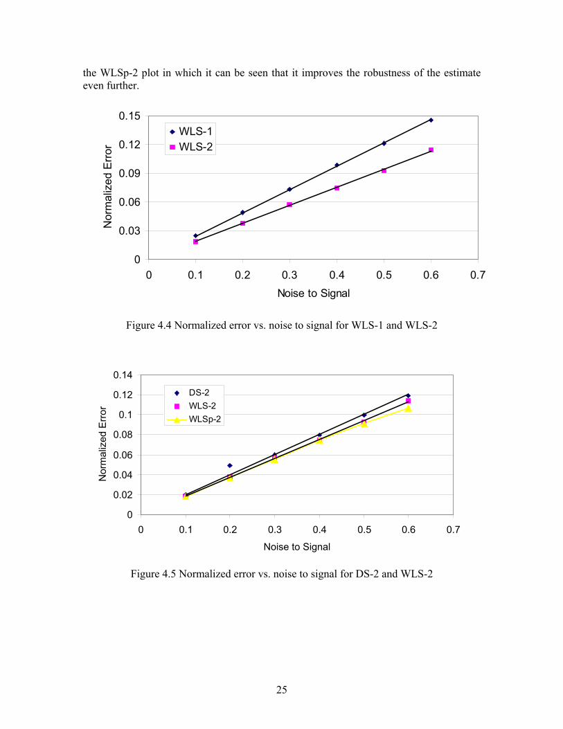
the WLSp-2 plot in which it can be seen that it improves the robustness of the estimate even further.

0

0.03

0.06

0.09

0.12

0.15

0 0.1 0.2 0.3 0.4 0.5 0.6 0.7Noise to Signal

Nor

mal

ized

Err

or

WLS-1WLS-2

Figure 4.4 Normalized error vs. noise to signal for WLS-1 and WLS-2

0

0.02

0.04

0.06

0.08

0.1

0.12

0.14

0 0.1 0.2 0.3 0.4 0.5 0.6 0.7

Noise to Signal

Nor

mal

ized

Err

or

DS-2WLS-2WLSp-2

Figure 4.5 Normalized error vs. noise to signal for DS-2 and WLS-2

25

4.6 Additional of PMU Measurements To further study the impact of PMUs measurements on the state estimation of the system, an examination the normalized error as the penetration of the PMU measurements continue to increase was done. The Figure 4.7 is the normalized error of augmenting the z vector with PMU measurements. The weights used were 100 for the PMU measurements and 0.3 for the non-PMU measurements. The noise to signal ration for non-PMU measurements is 0.3. The WLSp graph is that adjusted weighted least squares values. The graph indicates a negative exponential trend to the number of PMU added. As the penetration reaches high levels the amount of improvement in the state estimation is only decreasing less and less for each additional PMU.

y = 0.1249e-0.295x

R2 = 0.976

0

0.02

0.04

0.06

0.08

0.1

0.12

0.14

0.16

0 2 4 6 8 10 12 14Number of PMUs Used

Nor

mal

ized

Erro

r

WLSWLSp

Figure 4.6 Normalized error vs. number of PMUs added

The difference between the WLS and WLSp is expected as the penetration of PMUs increases. The WLS has estimates of the voltage phase angles measured by the PMU but the WLSp is adjusted by placing the values of voltage phase angle measurement in for PMU measured buses. This is a small difference in value per bus, but as the number of buses with PMUs increase so does the difference in norms.

26

4.7 Examination of the Variance of the E-vector

The error -xactual is now examined and this error is denominated as E. Note that this error is the true error in the state estimate – a quantity that is rarely known; however in this contrived example, the true value of the states is known, and therefore the true error is available. Note that E is a vector of the same dimension as x. The previous section examined the improvements in the normalized vector as the number of PMUs increase. The normalized error is

x̂

2

2ˆ

..actual

actual

xxx

EN−

=

and this quantity can now be written as

2

2..actualxE

EN = .

The E vector measures the difference between the estimate of x and the actual values. The noise in the system measurements is assumed to be normally distributed and thus the difference between the state estimate and the actual state is assumed to also be normally distributed.

At this point, consider the elements of vector E, namely {e1, e2, … , es}. Assume that the scalar mean of this ensemble is zero – an assumption that will be revisited later. The variance of {eI} is

s

es

ii

E

∑== 1

2

2σ .

When is replaced by the measurement made by the PMU as is the case in the adjusted weighted least squares method, then the ith element of E, namely ei, becomes zero. If there are g PMUs in the system, and the PMU measurements are assumed to be perfect, the Ecorrected vector is

ix̂

⎥⎥⎥⎥⎥⎥⎥⎥⎥

⎦

⎤

⎢⎢⎢⎢⎢⎢⎢⎢⎢

⎣

⎡

= −

0

0

2

1

Μ

Μ

gscorrected e

ee

E .

27

The variance of {ecorrected-I} is

s

egs

ii

Ecorrected

∑−

== 1

2

2σ ,

If s >> g, the sample the variance of {ecorrected-i} can be written as,

⎟⎠⎞

⎜⎝⎛ −=

sg

EEcorrected122 σσ . (4.1)

The variance of {ecorrected-i} is related to the L2 norm by

22 correctedEcorrected sE σ= .

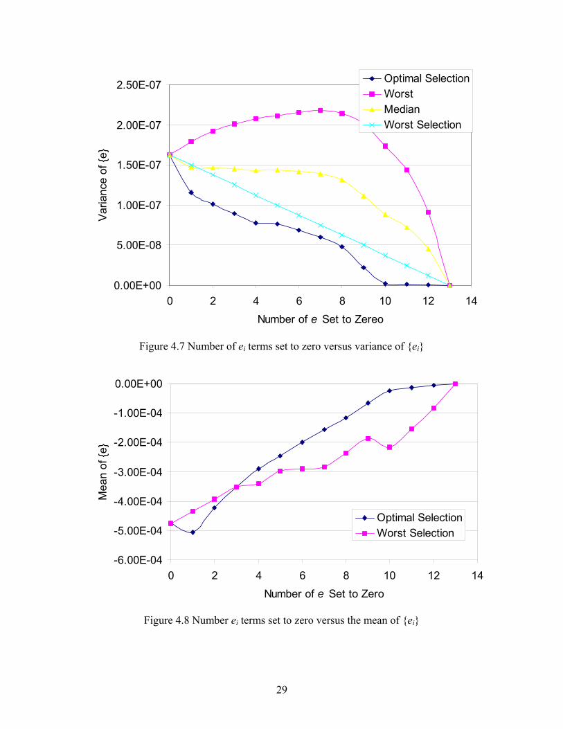
To investigate the validity of (4.1), consider the case when no PMUs are in the IEEE 14 bus system and the noise to signal ratio was (0.3) and examined. The sample mean of {ei} is -0.00048, which is in the same order of magnitude as all the elements ei. The variance of {ei} is 1.625E-7. The selection of which ei should be set to zero was determined by the difference of ei and the mean. Two cases were examined: 1) optimal selection case -- replacing the ei with the largest difference with zero and 2) worst selection case -- replacing the ei with the smallest difference with zero. Zeroing the largest ei is similar to placing the PMU at the bus which has the largest error between the estimate voltage phase angle and actual.

Figure 4.7 shows the results of the two cases studied and the predicted value using Equation (4.1). A reason for variation between the results and predicted values is that the mean of {ei} is not zero. Figure 4.8 shows that as ei are replaced with zeros, the mean of the remaining {ei} approaches zero.

The upper curve in 4.7 shows what will happen if the worst location for the PMU is chosen, and the lower curve shows the improvement which can be seen if best location is chosen based on reducing the variance of {ei}. The prediction line is a good approximation of the results in the improvement of the variance of {ei} if chosen with reason.

28

0.00E+00

5.00E-08

1.00E-07

1.50E-07

2.00E-07

2.50E-07

0 2 4 6 8 10 12 1Number of e Set to Zereo

Var

ianc

e of

{e}

4

Optimal SelectionWorstMedianWorst Selection

Figure 4.7 Number of ei terms set to zero versus variance of {ei}

-6.00E-04

-5.00E-04

-4.00E-04

-3.00E-04

-2.00E-04

-1.00E-04

0.00E+00

0 2 4 6 8 10 12 14Number of e Set to Zero

Mea

n of

{e}

Optimal SelectionWorst Selection

Figure 4.8 Number ei terms set to zero versus the mean of {ei}

29

4.8 Conclusions In this chapter it was examined the impacts of having multiple PMUs monitoring the system. The two primary methods used to incorporate the PMU voltage phase angle measurements into the system were direct substitution and weighted least squares. The weighted least squares were then adjusted after the state estimation to produce WLSp.

The weighted least squares method was shown to be better than direct substitution for the incorporating two PMU measurements into state estimation. A drawback about the weighted least squares method was as the noise level varied the optimal location of the two PMUs varied, which was not observed with the direct substitution method. The post state estimation replacement of the estimated state with the PMU measurement also allowed for lower normalized error even further. The cases of when the noise to signal ratio was large and when the penetration of the PMU measurements in the system was high, the adjusted weighted least squares estimate was best. This is due to the fact that the adjusted weighted least squares estimate removed any error that was present in the estimate of phase angle in which was measured by a PMU.

30

5. Conclusions and Future Work

5.1 Conclusions In Chapter 3 the case of placing one PMU in a power system was examined. Two primary methods used to incorporate the PMU measurements into the state estimation. One was to add the measurements to the weighted least squares method as an additional measurement with significant weight compared. The other method is to eliminate the equations that correspond to the respective phase, that is direct substitution. Both methods showed significant improvement in the voltage angle estimate with the incorporation of one PMU measurement. The method of direct substitution did produce a smaller normalized error for the noise to signal ratio of (0.3). However, on the basis of limited experimentation with the IEEE 14 bus system, it is concluded that to include one PMU measurement, it is better (i.e., more accurate estimate) to use weighted least squares rather than direct substitution.

When the noise to signal ratio is varied, the plots of the normalized error for the method direct substitution, the method of augmenting the weighted least squares, and the method of adjusted weighted least squares appear to exhibit similar accuracy. The experiment of replacing the weighted least squares estimate with the PMU measurement after the state estimation did not result in significant improvement in the normalized error. This is to be expected when the difference between the estimate and the actual voltage phase angle measurement is small. Also in the series of experiments presented in Chapter 3 there was only one PMU added thus the change in estimate and adjusted estimate would be small. For all levels of noise, there were still significant improvements in the state estimation by incorporating just one PMU into the system.

Chapter 4 examined the impacts of having multiple PMUs monitoring the system. The two primary methods used to incorporate the PMU voltage phase angle measurements into the system were direct substitution and weighted least squares. As an additional test, the weighted least squares estimate corresponding to PMU measurements were discarded and replaced by the PMU measurements after the state estimation to produce a test series denoted WLSp.

The weighted least squares method was shown to be better than direct substitution for incorporating two PMU measurements into the state estimation. This conclusion applies at all levels of noise tested. A drawback of the weighted least squares method is that the optimal location of the two PMUs is dependent on the noise level. This is not observed using direct substitution. The post state estimation adjustment (i.e., discard estimate and replace with PMU measurement) to state vector also allowed for lower normalized error. The cases in which the noise to signal ratio was large and when the penetration of the PMU measurements in the system was high, the weighted least squares estimate with replacement of estimates with PMU measurements was best.

The general conclusion, on the basis of tests done, indicates that the weighted least squares method of incorporating PMU voltage phase angle measurements into the state estimate is the most versatile. The weighted least squares method allows for significant

31

weight to be placed on the measurements made by the PMUs; the direct substitution method holds the value of the bus voltage phase angle measured. The weighted least squares method allows freedom of the estimator to adjust the values of the bus angle measurements to minimize ||Hx-z||2, which is a feature that direct substitution does not exhibit. The post estimation adjustment of the bus angles with PMU data to measured values does provide lower normalized error than retaining the estimated phase angles. This ‘correction’ may not be significant except in cases of high measurement error or high penetration of PMUs.

5.2 Future Work The work done in this report has made advancements in the selection of optimal placement of PMUs and the incorporation of the PMU measurements into the state estimator but there is still more work that could be done in this area. Some of the topics that would help in the advancement in topics of studied in this report are:

• Much larger tests • Include magnitude of voltage in the state estimation • Further attempt at the analysis of equations to obtain mathematically analytic

expression of error reduction due to PMU measurement use • Affects of correlated (common mode) noise • The effect of nonsimultaneous measurements in systems with PMU

measurements • System totally monitored by PMUs no state estimation • Cost-benefit analysis of adding “one more” PMU.

The work done was on a 14 bus system, would similar results come from a study of the 57 bus system? The work was of the linear equation of power flow voltage what impact would including the voltage magnitude have on the state estimation with PMU devices. In this report there was an examination of the least squares bounds as described in [14]. But the least square bounds were not comparable to the results of the experiments further examination should be made. The noise used in the report was pseudorandom noise independent from noise at other buses, what happens when the noise at buses are correlated on each other? Experiments WSL-13-0.3 and WLSp-13-0.3 looked at the case of having the system totally monitored by PMUs what are the benefits and costs of doing this.

32

REFERENCES

[1] E. Iwata, “Report faults Ohio utility,” USA Today, November 20, 2003, pp. 1A. [2] F. Schweppe, J. Wildes, D. Rom, “Power system static state estimation: parts I, II,

and III,” Power Industry Computer Conference, June 1969. [3] P. Zarco, A. Exposito, “Power system parameter estimation: survey” IEEE

Transactions on Power Systems, Vol. 15, No. 1, February 2000, pp. 216-222. [4] M. E. El-Hawary, “Bad data detection of unequal magnitudes in state estimation of

power systems,” IEEE Power Engineering Review, Vol. 22, No. 4, April 2002, pp. 57-60.

[5] B. Gou, A. Abur, “An improved measurement placement algorithm for network observability,” IEEE Transactions on Power Systems, Vol. 16, No. 4, November 2001, pp 819-824.

[6] A. Monticelli, State Estimation in Electric Power Systems, Boston, Kluwer Academic Publishers,1999.

[7] A. J. Wood, B. F. Wollenberg, Power Generation Operation and Control, New York, Wiley, 1984.

[8] F. C. Schweppe, Uncertain Dynamic Systems, Prentice-Hall, 1973. [9] A. Abur, A. G. Exposito, Power System State Estimation: Theory and

Implementation, New York, Marcel Dekker, 2004 [10] I. O. Habiballah, “Modified two-level state estimation approach [for power systems],”

IEE Proceedings on Generation, Transmission and Distribution, Vol. 143, No. 2, March 1996, pp. 193-199.

[11] A. Monticelli, “Electric power system state estimation,” Proceedings of the IEEE, Vol. 88, No. 2, Feb. 2000 pp. 262 – 282.

[12] J. B. Carvalho, F. M. Barbosa, “A modern state estimation in power system energy.” International Conference on Electric Power Engineering, 1999 PowerTech Budapest 99, Sept. 1999, pp. 270.

[14] O. Alsac, N. Vempati, B. Stott, A. Montilcelli, “Generalized state estimation,” IEEE Transactions on Power Systems, Vol. 13, No. 3, Aug. 1998 pp. 1069 – 1075.

[15] M. V. F. Pereia, N. J. Balu, “Composite generation/transmission reliability evaluation,” Proceedings of the IEEE, Vol. 80, No. 4, April 1992, pp. 470 – 491.

[16] G. H. Golub, C. F. Van Loan, Matrix Computations, Baltimore, Johns Hopkins University Press, 1983.

[17] K. Chow, J. Shin, S. Hyun, “Optimal placement of phasor measurement units with GPS receiver,” Proceedings of the Power Engineering Society Winter Meeting, Vol. 1, January 2001, pp. 258-262.

[18] A. G. Phadke, “Synchronized phasor measurements ~ a historical overview,” Proceedings of the Transmission and Distribution Conference and Exhibition 2002: Asia/Pacific, Vol. 1, Oct 2002, pp. 476-479.

33

[19] W. Lewandowski, J. Asoubib, W. J. Klepczynski, “GPS: primary tool for time transfer,” Proceedings of the IEEE, Vol. 87, No. 1. Jan. 1999, pp. 163-172.

[20] B. Milosevic, M. Begovic, “Nondominated sorting genetic algorithm for optimal phasor measurement placement,” IEEE Transactions on Power Systems, Vol. 18, No. 1, February 2003, pp. 69-75.

[21] G. B. Denergi, M. Invernizzi, F. Milano, M. Fiorina, P. Scarpellini, “A security oriented approach to PMU positioning for advance monitoring of a transmission grid,” Proceedings of the International Conference on Power System Technology, Vol. 2, October 2002, pp. 798-803.

[22] R. Zivanovic, C. Cairns, “Implementation of PMU technology in state estimation: an overview,” IEEE AFRICON 4th, Vol. 2, September 1996, pp. 1006-1011.

[23] I. Kamwa, R. Grondin, “PMU configuration for system dynamic performance measurement in large multiarea power systems,” IEEE Transactions on Power Systems, Vol. 17, No. 2 May 2002, pp. 385-394.

[24] A.G. Phadke, B. Pickett, M. Adamiak, M. Begovic, G. Benmouyal, R. O. Burnett, Jr., T.W. Cease, J. Goossens, D. J. Hansen, M. Kezunovic, L. L. Mankoff, P. G. McLaren, G. Michel, R. J. Murphy, J. Nordstrom, M. S. Sachdev, H. S. Smith, J. S. Thorp, M. Trotignon, T. C. Wang, M. A. Xavier, “Synchronized sampling and phasor measurements for relaying and control,” IEEE Transactions on Power Delivery, Vol. 9, No. 1, 1994, pp. 442-452.

[25] R. Christie, “Power System Test Archive” http://www.ee.washington.edu/research/pstca/pf14/pg_tca14bus.htm.

34

A. IEEE14 Bus Test Bed System Information

Table A.1 Solved delta values for IEEE 14 bus system

Bus Delta Number (radians)

2 -0.086923 -0.222014 -0.180295 -0.153246 -0.248197 -0.233358 -0.233189 -0.2607510 -0.2635411 -0.2581312 -0.2630213 -0.2645914 -0.27995

35

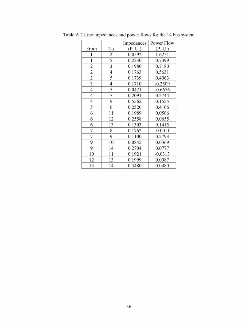
Table A.2 Line impedances and power flows for the 14 bus system

From To Impedances

(P. U.) Power Flow

(P. U.) 1 2 0.0592 1.6251 1 5 0.2230 0.7399 2 3 0.1980 0.7180 2 4 0.1763 0.5631 2 5 0.1739 0.4063 3 4 0.1710 -0.2509 4 5 0.0421 -0.6676 4 7 0.2091 0.2744 4 9 0.5562 0.1555 5 6 0.2520 0.4106 6 11 0.1989 0.0566 6 12 0.2558 0.0655 6 13 0.1303 0.1415 7 8 0.1762 -0.0011 7 9 0.1100 0.2793 9 10 0.0845 0.0369 9 14 0.2704 0.0777 10 11 0.1921 -0.0313 12 13 0.1999 0.0087 13 14 0.3480 0.0480

36

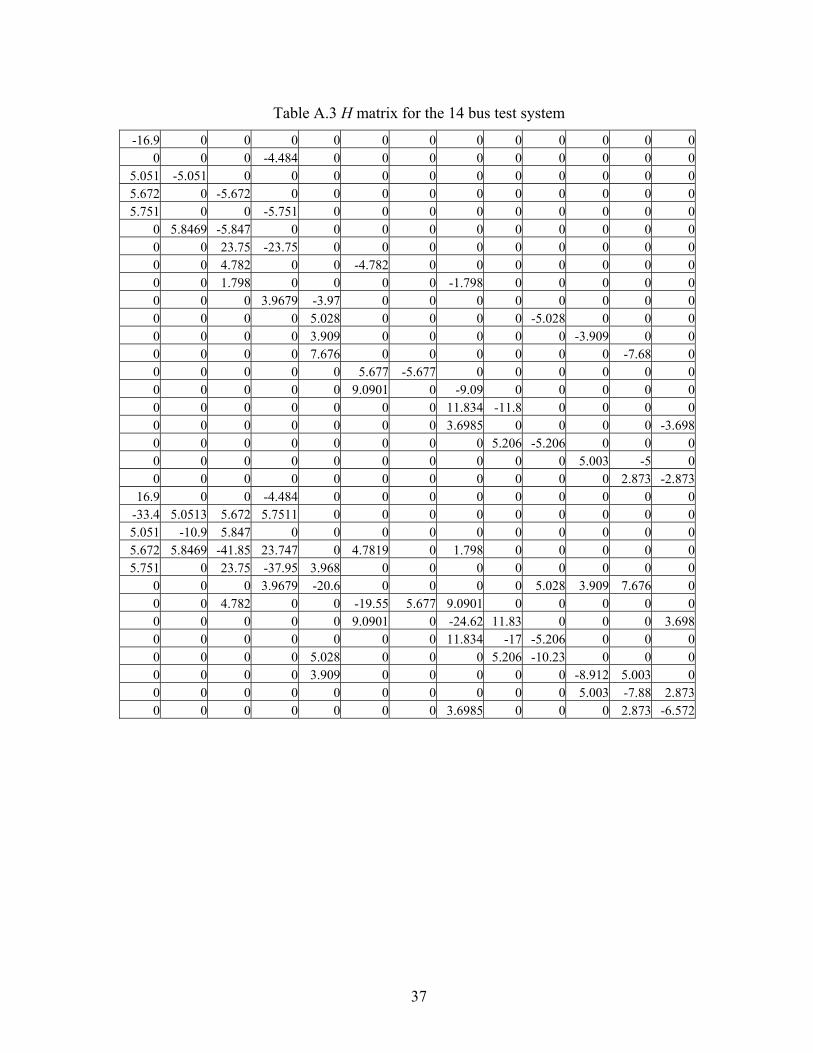
Table A.3 H matrix for the 14 bus test system

-16.9 0 0 0 0 0 0 0 0 0 0 0 00 0 0 -4.484 0 0 0 0 0 0 0 0 0

5.051 -5.051 0 0 0 0 0 0 0 0 0 0 05.672 0 -5.672 0 0 0 0 0 0 0 0 0 05.751 0 0 -5.751 0 0 0 0 0 0 0 0 0

0 5.8469 -5.847 0 0 0 0 0 0 0 0 0 00 0 23.75 -23.75 0 0 0 0 0 0 0 0 00 0 4.782 0 0 -4.782 0 0 0 0 0 0 00 0 1.798 0 0 0 0 -1.798 0 0 0 0 00 0 0 3.9679 -3.97 0 0 0 0 0 0 0 00 0 0 0 5.028 0 0 0 0 -5.028 0 0 00 0 0 0 3.909 0 0 0 0 0 -3.909 0 00 0 0 0 7.676 0 0 0 0 0 0 -7.68 00 0 0 0 0 5.677 -5.677 0 0 0 0 0 00 0 0 0 0 9.0901 0 -9.09 0 0 0 0 00 0 0 0 0 0 0 11.834 -11.8 0 0 0 00 0 0 0 0 0 0 3.6985 0 0 0 0 -3.6980 0 0 0 0 0 0 0 5.206 -5.206 0 0 00 0 0 0 0 0 0 0 0 0 5.003 -5 00 0 0 0 0 0 0 0 0 0 0 2.873 -2.873

16.9 0 0 -4.484 0 0 0 0 0 0 0 0 0-33.4 5.0513 5.672 5.7511 0 0 0 0 0 0 0 0 05.051 -10.9 5.847 0 0 0 0 0 0 0 0 0 05.672 5.8469 -41.85 23.747 0 4.7819 0 1.798 0 0 0 0 05.751 0 23.75 -37.95 3.968 0 0 0 0 0 0 0 0

0 0 0 3.9679 -20.6 0 0 0 0 5.028 3.909 7.676 00 0 4.782 0 0 -19.55 5.677 9.0901 0 0 0 0 00 0 0 0 0 9.0901 0 -24.62 11.83 0 0 0 3.6980 0 0 0 0 0 0 11.834 -17 -5.206 0 0 00 0 0 0 5.028 0 0 0 5.206 -10.23 0 0 00 0 0 0 3.909 0 0 0 0 0 -8.912 5.003 00 0 0 0 0 0 0 0 0 0 5.003 -7.88 2.8730 0 0 0 0 0 0 3.6985 0 0 0 2.873 -6.572

37

B. MATLAB Scripts for State Estimation

B.1 Script for a Single PMU in the 14 Bus System %///////////////////////////////////////////////////% % Mark Rice % % May 13,2004 % % ASU Research % % % % Look at the RMS of Error in X when States are % % known Now Examing the IEEE 14 bus system % %///////////////////////////////////////////////////% clear; % Number of Buses is 14 % Number of Measurments is ???? X=[ -0.086917397; -0.222005881; -0.180292512; -0.153239908; -0.24818582; -0.233350521; -0.233175988; -0.26075219; -0.263544717; -0.258134196; -0.263021118; -0.264591915; -0.279950812]; H=[-16.90045631 0 0 0 0 0 0 0 0 0 0 0 0; 0 0 0 -4.483500717 0 0 0 0 0 0 0 0 0; 5.051270395 -5.051270395 0 0 0 0 0 0 0 0 0 0 0; 5.671506352 0 -5.671506352 0 0 0 0 0 0 0 0 0 0; 5.751092708 0 0 -5.751092708 0 0 0 0 0 0 0 0 0;

38

0 5.84692744 -5.84692744 0 0 0 0 0 0 0 0 0 0; 0 0 23.74732843 -23.74732843 0 0 0 0 0 0 0 0 0; 0 0 4.781943382 0 0 -4.781943382 0 0 0 0 0 0 0; 0 0 1.797979072 0 0 0 0 -1.797979072 0 0 0 0 0; 0 0 0 3.967939052 -3.967939052 0 0 0 0 0 0 0 0; 0 0 0 0 5.027652086 0 0 0 0 -5.027652086 0 0 0; 0 0 0 0 3.909151323 0 0 0 0 0 -3.909151323 0 0; 0 0 0 0 7.676364474 0 0 0 0 0 0 -7.676364474 0; 0 0 0 0 0 5.676979847 -5.676979847 0 0 0 0 0 0; 0 0 0 0 0 9.09008272 0 -9.09008272 0 0 0 0 0; 0 0 0 0 0 0 0 11.83431953 -11.83431953 0 0 0 0; 0 0 0 0 0 0 0 3.69849841 0 0 0 0 -3.69849841; 0 0 0 0 0 0 0 0 5.206435154 -5.206435154 0 0 0; 0 0 0 0 0 0 0 0 0 0 5.003001801 -5.003001801 0; 0 0 0 0 0 0 0 0 0 0 0 2.873398081 -2.873398081 16.90045631 0 0 -4.483500717 0 0 0 0 0 0 0 0 0; -33.37432577 5.051270395 5.671506352 5.751092708 0 0 0 0 0 0 0 0 0; 5.051270395 -10.89819783 5.84692744 0 0 0 0 0 0 0 0 0 0; 5.671506352 5.84692744 -41.84568467 23.74732843 0 4.781943382 0 1.797979072 0 0 0 0 0; 5.751092708 0 23.74732843 -37.9498609 3.967939052 0 0 0 0 0 0 0 0; 0 0 0 3.967939052 -20.58110694 0 0 0 0 5.027652086 3.909151323 7.676364474 0; 0 0 4.781943382 0 0 -19.54900595 5.676979847 9.09008272 0 0 0 0 0;

39

0 0 0 0 0 9.09008272 0 -24.62290066 11.83431953 0 0 0 3.69849841; 0 0 0 0 0 0 0 11.83431953 -17.04075468 -5.206435154 0 0 0; 0 0 0 0 5.027652086 0 0 0 5.206435154 -10.23408724 0 0 0; 0 0 0 0 3.909151323 0 0 0 0 0 -8.912153124 5.003001801 0; 0 0 0 0 0 0 0 0 0 0 5.003001801 -7.876399882 2.873398081; 0 0 0 0 0 0 0 3.69849841 0 0 0 2.873398081 -6.57189649]; Z=[ 1.46894367057742 0.68705123739101 0.68236845993463 0.52957755784123 0.38142690938835 -0.24389504182095 -0.64242707207473 0.25372039499965 0.14466481718386 0.37673959205256 0.05001697334871 0.05799342480380 0.12593916481507 -0.00099082032364 0.24908343787606 0.03304765681415 0.07100607294119 -0.02816952673586 0.00785870022001 0.04413222516608 -0.78189243318641 -0.12442925615220 0.92626350064555 0.52972437482976 0.04931148157940 0.14279003032591 0.00562777768057 0.14502970812072 2.74913508750368 0.02184744661286 0.05013472458379 -0.03627352494607

40

0.11513829782732]; %/ Noise set at 30% % Noiselist=[.1,.2,.3,.4,.5,.6,.7,.8,.9,1]; for n=1:size(Noiselist,2) noise=Noiselist(n); Stored=0; Uppers=0; trials=1000; s=size(X); sizex=s(1,1) KA=cond(H); stNXP=0; stSw=0; stNXPw=0; StoreEX=0; SizeZ=size(Z); counter1=0; % Creation of the covariance Matrix W=(0.3)^2*eye(SizeZ(1,1)); for i=1:trials eta=noise*(randn(SizeZ(1,1),1)).*Z; Zn=Z+eta; Xhat1=pinv(H)*Zn; %Ex=X-Xhat1; %StoreEX=StoreEX+abs(Ex); %Ex2=Ex.*Ex; %S=sqrt(sum(Ex2)/(s(1,1))); %Stored=Stored+S; %Rhols=norm(H*Xhat1-Zn); %theta=asin(Rhols/norm(Z)); %Upper=(norm(eta)/norm(Z))*(2*KA/cos(theta)+tan(theta)*cond(transpose(H)*H)); %Uppers=Uppers+Upper; NXP=norm(X-Xhat1)/norm(X); stNXP=stNXP+NXP; %Now Time to examine the happenings of WLS XhatW=(transpose(H)*W*H)^-1*transpose(H)*W*Zn; NXPw=norm(X-XhatW)/norm(X); %Sw=sqrt((transpose(X-XhatW)*(X-XhatW))/s(1,1)); stNXPw=NXPw+stNXPw;

41

%stSw=Sw+stSw; %counter1=counter1+1; end %NormXp=norm(X); %AvgEX=StoreEX/trials; %ExpS=Stored/trials; %UpperB=Uppers/trials; AvgNXP(1,n)=stNXP/trials; %AvgWerror=stSw/trials; AvgNXPw(1,n)=stNXPw/trials; %counter2=0; %counter3=0; %NormHds(1,1)=norm(transpose(H)*H) %NormHwls(1,1)=norm(transpose(H)*W*H) %Examining Condition Numbers %KAds=KA; %KAwls=cond(sqrt(W)*H); %now time to examine what happens when one of the states is known.% Ws=(0.3)*eye(SizeZ(1,1)+1); Ws(1,1)=100; for k=1:sizex Hp=H; Xp=X; H1=H(:,k); X1=X(k,1); Zp=Z; % Zp=Z-H1*X1; SizeZp=size(Zp); Hp(:,k)=[]; Xp(k,:)=[]; sp=size(Xp); Storedp=0; KA=cond(Hp); stNXP=0;

42

Uppers=0; stNormR=0; stNXPwp=0; %Routine for the Creation of adding a precise Measurement to WLS Hw=H; [height,width]=size(Hw); Hw=[zeros(1,width);Hw]; Hw(1,k)=1; stSw=0; stNXPw=0; %somethting Funky sTdeltaX=0; % investigating changes in H %NormHds(k+1,1)=norm(transpose(Hp)*Hp); %NormHwls(k+1,1)=norm(transpose(Hw)*Ws*Hw); % Examining Condtion Number %KAds(k+1,1)=cond(Hp); %KAwls(k+1,1)=cond(sqrt(Ws)*Hw); for i=1:trials eta=noise*(randn(SizeZp(1,1),1)).*Zp; Zn=Zp+eta; Zn=Zn-X1*H1; %Allows the noise to be just on the measurmentent Xhat=pinv(Hp)*Zn; Ex=Xp-Xhat; Ex2=Ex.*Ex; Sp=norm(Xp-Xhat)/norm(Xp); Storedp=Storedp+Sp; %normR=norm(Hp*Xhat-Zn); %stNormR=stNormR+normR; % Finding the Bound Limits %Rhols=norm(Hp*Xhat-Zn); %theta=asin(Rhols/norm(Zp));

43

%Upper=(norm(eta)/norm(Zp))*(2*cond(Hp)/cos(theta)+tan(theta)*cond(transpose(Hp)*Hp)); %Uppers=Uppers+Upper; NXP=norm(Xp-Xhat)/norm(Xp); stNXP=stNXP+NXP; %Finding the WLS Solution Zw=[X(k);Z+noise*randn(size(Z)).*Z]; XhatW=(transpose(Hw)*Ws*Hw)^-1*transpose(Hw)*Ws*Zw; NXPw=norm(X-XhatW)/norm(X); Sw=sqrt((transpose(X-XhatW)*(X-XhatW))/s(1,1)); stNXPw=NXPw+stNXPw; stSw=Sw+stSw; XhatWp=XhatW; XhatWp(k)=X1; NXPwp=norm(X-XhatWp)/norm(X); stNXPwp=NXPwp+stNXPwp; %B/c I am clueless Lets examining the change in Error at each of the busses %sTdeltaX=sTdeltaX+abs(Xp-Xhat); %counter2=counter2+1; end %ExpS(k+1,1)=Storedp/trials; %UpperB(k+1,1)=Uppers/trials; AvgNXP(k+1,n)=stNXP/trials; %AvgWerror(k+1,1)=stSw/trials; AvgNXPw(k+1,n)=stNXPw/trials; %NormXp(k+1)=norm(Xp); %AvgR(k)=stNormR/trials; AvgNXPwp(k,n)=stNXPwp/trials; %attempting to atribute the Correct changes in X to the right place %AvgEXp=sTdeltaX/trials; %Avgerrorp(:,k)=AvgEXp; %l=0; %j=0; %while l<12 % l=l+1; % j=j+1; % if j==k

44

% AvgEx(j,k)=0; % j=j+1; % end % AvgEx(j,k)=AvgEXp(l,1); %end %counter3=counter3+1; end end %ExpS %Lexps=-log10(ExpS); % M=[0:1:s(1,1)]; %figure %bar(M,ExpS) %title('RMS Error of X') % figure % bar(M,AvgNXP); % title('Avg Error in X') %figure %bar(M,UpperB) %title('Bounds as H changes') % figure % bar(M,AvgNXPw) % title('WLS error') %figure %bar(M,NormXp) %title('Norm of Xp') %figure %bar(AvgR) %title('Residual of Direct Subsitution')

B.2 Script for Examining Two PMU in the 14 Bus System %///////////////////////////////////////////////////% % Mark Rice % % May 13,2004 % % ASU Research %

45

% % % Look at the RMS of Error in X when States are % % known Now Examing the IEEE 14 bus system % %///////////////////////////////////////////////////% clear; % Number of Buses is 14 % Number of Measurments is ???? X=[ -0.086917397; -0.222005881; -0.180292512; -0.153239908; -0.24818582; -0.233350521; -0.233175988; -0.26075219; -0.263544717; -0.258134196; -0.263021118; -0.264591915; -0.279950812]; H=[-16.90045631 0 0 0 0 0 0 0 0 0 0 0 0; 0 0 0 -4.483500717 0 0 0 0 0 0 0 0 0; 5.051270395 -5.051270395 0 0 0 0 0 0 0 0 0 0 0; 5.671506352 0 -5.671506352 0 0 0 0 0 0 0 0 0 0; 5.751092708 0 0 -5.751092708 0 0 0 0 0 0 0 0 0; 0 5.84692744 -5.84692744 0 0 0 0 0 0 0 0 0 0; 0 0 23.74732843 -23.74732843 0 0 0 0 0 0 0 0 0; 0 0 4.781943382 0 0 -4.781943382 0 0 0 0 0 0 0; 0 0 1.797979072 0 0 0 0 -1.797979072 0 0 0 0 0; 0 0 0 3.967939052 -3.967939052 0 0 0 0 0 0 0 0;

46

0 0 0 0 5.027652086 0 0 0 0 -5.027652086 0 0 0; 0 0 0 0 3.909151323 0 0 0 0 0 -3.909151323 0 0; 0 0 0 0 7.676364474 0 0 0 0 0 0 -7.676364474 0; 0 0 0 0 0 5.676979847 -5.676979847 0 0 0 0 0 0; 0 0 0 0 0 9.09008272 0 -9.09008272 0 0 0 0 0; 0 0 0 0 0 0 0 11.83431953 -11.83431953 0 0 0 0; 0 0 0 0 0 0 0 3.69849841 0 0 0 0 -3.69849841; 0 0 0 0 0 0 0 0 5.206435154 -5.206435154 0 0 0; 0 0 0 0 0 0 0 0 0 0 5.003001801 -5.003001801 0; 0 0 0 0 0 0 0 0 0 0 0 2.873398081 -2.873398081 16.90045631 0 0 -4.483500717 0 0 0 0 0 0 0 0 0; -33.37432577 5.051270395 5.671506352 5.751092708 0 0 0 0 0 0 0 0 0; 5.051270395 -10.89819783 5.84692744 0 0 0 0 0 0 0 0 0 0; 5.671506352 5.84692744 -41.84568467 23.74732843 0 4.781943382 0 1.797979072 0 0 0 0 0; 5.751092708 0 23.74732843 -37.9498609 3.967939052 0 0 0 0 0 0 0 0; 0 0 0 3.967939052 -20.58110694 0 0 0 0 5.027652086 3.909151323 7.676364474 0; 0 0 4.781943382 0 0 -19.54900595 5.676979847 9.09008272 0 0 0 0 0; 0 0 0 0 0 9.09008272 0 -24.62290066 11.83431953 0 0 0 3.69849841; 0 0 0 0 0 0 0 11.83431953 -17.04075468 -5.206435154 0 0 0; 0 0 0 0 5.027652086 0 0 0 5.206435154 -10.23408724 0 0 0; 0 0 0 0 3.909151323 0 0 0 0 0 -8.912153124 5.003001801 0; 0 0 0 0 0 0 0 0 0 0 5.003001801 -7.876399882 2.873398081;

47

0 0 0 0 0 0 0 3.69849841 0 0 0 2.873398081 -6.57189649]; Z=[ 1.46894367057742 0.68705123739101 0.68236845993463 0.52957755784123 0.38142690938835 -0.24389504182095 -0.64242707207473 0.25372039499965 0.14466481718386 0.37673959205256 0.05001697334871 0.05799342480380 0.12593916481507 -0.00099082032364 0.24908343787606 0.03304765681415 0.07100607294119 -0.02816952673586 0.00785870022001 0.04413222516608 -0.78189243318641 -0.12442925615220 0.92626350064555 0.52972437482976 0.04931148157940 0.14279003032591 0.00562777768057 0.14502970812072 2.74913508750368 0.02184744661286 0.05013472458379 -0.03627352494607 0.11513829782732]; %/ Noise set at 30% % noise=.6; Stored=0; Uppers=0; trials=5000; s=size(X); sizex=s(1,1) KA=cond(H);

48

stNXP=0; stSw=0; stNXPw=0; StoreEX=0; SizeZ=size(Z); counter1=0; % Creation of the covariance Matrix W=(.3)^2*eye(SizeZ(1,1)); Ws=(.3)*eye(SizeZ(1,1)+1); Ws(1,1)=100; % buslist=[2 3 4 5 6 7 8 9 10 11 12 13 14]; % Creation of the Base of 8 has a PMU on it % for bus=1:13 % buslistd=buslist; PMU=10; % buslistd(PMU)=[]; Hptwo=H; Xptwo=X; H1two=H(:,PMU); HPMU1=H1two; X1two=X(PMU,1); XPMU1=X1two; Zptwo=Z; SizeZptwo=size(Zptwo); Hptwo(:,PMU)=[]; Xptwo(PMU,:)=[]; Hwtwo=H; [height,width]=size(Hwtwo); Hwtwo=[zeros(1,width);Hwtwo]; Hwtwo(1,PMU)=1; % % for i=1:trials % eta=noise*(randn(SizeZ(1,1),1)).*Z; % Zn=Z+eta; % Zn=Zn-X1two*H1two; % Xhat1=pinv(Hptwo)*Zn; % %Ex=Xptwo-Xhat1; % %StoreEX=StoreEX+abs(Ex); % %Ex2=Ex'*Ex; % %S=sqrt((Ex2)/(s(1,1))); % %Stored=Stored+S; % %Rhols=norm(H*Xhat1-Zn);

49

% %theta=asin(Rhols/norm(Z)); % %Upper=(norm(eta)/norm(Z))*(2*KA/cos(theta)+tan(theta)*cond(transpose(H)*H)); % %Uppers=Uppers+Upper; % NXP=norm(Xptwo-Xhat1)/norm(Xptwo); % stNXP=stNXP+NXP; % % %Now Time to examine the happenings of WLS % % Zw=[X(PMU);Z+noise*randn(size(Z)).*Z]; % XhatW=(transpose(Hwtwo)*Ws*Hwtwo)^-1*transpose(Hwtwo)*Ws*Zw; % NXPw=norm(X-XhatW)/norm(X); % stNXPw=stNXPw+NXPw; % % counter1=counter1+1; % % end % % %NormXp=norm(X); % %AvgEX=StoreEX/trials; % %ExpS=Stored/trials; % %UpperB=Uppers/trials; % AvgNXP=stNXP/trials; % %AvgWerror=stSw/trials; % AvgNXPw=stNXPw/trials; %counter2=0; %counter3=0; %NormHds(1,1)=norm(transpose(H)*H) %NormHwls(1,1)=norm(transpose(H)*W*H) %Examining Condition Numbers %KAds=KA; %KAwls=cond(sqrt(W)*H); %now time to examine what happens when one of the states is known.% Ws=(noise)*eye(SizeZ(1,1)+2); Ws(2,2)=100; Ws(1,1)=100; k=1; s=size(Xptwo); sizex=s(1,1)

50

for k=1:sizex Hp=Hptwo; Xp=Xptwo; H1=Hp(:,k); X1=Xp(k,1); Zp=Z; SizeZp=size(Zp); Hp(:,k)=[]; Xp(k,:)=[]; sp=size(Xp); Storedp=0; %KA=cond(Hp); stNXP=0; %ppers=0; %stNormR=0; %Routine for the Creation of adding a precies Measurement to WLS Hw=Hwtwo; [height,width]=size(Hw); Hw=[zeros(1,width);Hw]; Hw(1,k)=1; stSw=0; stNXPw=0; stNXPwp=0; for i=1:trials eta=noise*(randn(SizeZp(1,1),1)).*Zp; Zn=Zp+eta; Zn=Zn-X1*H1-XPMU1*HPMU1; %Allows the noise to be just on the measurmentent Xhat=pinv(Hp)*Zn; Ex=Xp-Xhat; NXP=norm(Xp-Xhat)/norm(Xp); stNXP=stNXP+NXP; %Finding the WLS Solution Zw=[X(k);X(PMU);Z+noise*randn(size(Z)).*Z]; XhatW=(transpose(Hw)*Ws*Hw)^-1*transpose(Hw)*Ws*Zw;

51

NXPw=norm(X-XhatW)/norm(X); %Sw=sqrt((transpose(X-XhatW)*(X-XhatW))/s(1,1)); stNXPw=NXPw+stNXPw; %stSw=Sw+stSw; XhatWp=XhatW; XhatWp(PMU)=X(PMU); XhatWp(k)=X(k); NXPwp=norm(XhatWp-X)/norm(X); stNXPwp=stNXPwp+NXPwp; end %ExpS(k+1,1)=Storedp/trials; %UpperB(k+1,1)=Uppers/trials; AvgNXP(k+1,1)=stNXP/trials; %AvgWerror(k+1,1)=stSw/trials; AvgNXPw(k+1,1)=stNXPw/trials; %NormXp(k+1)=norm(Xp); %AvgR(k)=stNormR/trials; AvgNXPwp(k,1)=stNXPwp/trials; %attempting to atribute the Correct changes in X to the right place %AvgEXp=sTdeltaX/trials; %Avgerrorp(:,k)=AvgEXp; %l=0; %j=0; %while l<12 % l=l+1; % j=j+1; % if j==k % AvgEx(j,k)=0; % j=j+1; % end % AvgEx(j,k)=AvgEXp(l,1); %end end % [NEd(bus),bus2d]=min(AvgNXP); % [NEw(bus),bus2w]=min(AvgNXPw); % [NEp(bus),bus2p]=min(AvgNXPwp); % Bus2d(bus)=buslistd(bus2d); % Bus2w(bus)=buslist(bus2w);

52

% Bus2p(bus)=buslist(bus2p); % end

B.3 Script to Examine Impact of Multiple PMUs on the 14 Bus System

clear; % Number of Buses is 14 % Number of Measurments is ???? X=[ -0.086917397; -0.222005881; -0.180292512; -0.153239908; -0.24818582; -0.233350521; -0.233175988; -0.26075219; -0.263544717; -0.258134196; -0.263021118; -0.264591915; -0.279950812]; H=[-16.90045631 0 0 0 0 0 0 0 0 0 0 0 0; 0 0 0 -4.483500717 0 0 0 0 0 0 0 0 0; 5.051270395 -5.051270395 0 0 0 0 0 0 0 0 0 0 0; 5.671506352 0 -5.671506352 0 0 0 0 0 0 0 0 0 0; 5.751092708 0 0 -5.751092708 0 0 0 0 0 0 0 0 0; 0 5.84692744 -5.84692744 0 0 0 0 0 0 0 0 0 0; 0 0 23.74732843 -23.74732843 0 0 0 0 0 0 0 0 0; 0 0 4.781943382 0 0 -4.781943382 0 0 0 0 0 0 0; 0 0 1.797979072 0 0 0 0 -1.797979072 0 0 0 0 0; 0 0 0 3.967939052 -3.967939052 0 0 0 0 0 0 0 0;

53

0 0 0 0 5.027652086 0 0 0 0 -5.027652086 0 0 0; 0 0 0 0 3.909151323 0 0 0 0 0 -3.909151323 0 0; 0 0 0 0 7.676364474 0 0 0 0 0 0 -7.676364474 0; 0 0 0 0 0 5.676979847 -5.676979847 0 0 0 0 0 0; 0 0 0 0 0 9.09008272 0 -9.09008272 0 0 0 0 0; 0 0 0 0 0 0 0 11.83431953 -11.83431953 0 0 0 0; 0 0 0 0 0 0 0 3.69849841 0 0 0 0 -3.69849841; 0 0 0 0 0 0 0 0 5.206435154 -5.206435154 0 0 0; 0 0 0 0 0 0 0 0 0 0 5.003001801 -5.003001801 0; 0 0 0 0 0 0 0 0 0 0 0 2.873398081 -2.873398081 16.90045631 0 0 -4.483500717 0 0 0 0 0 0 0 0 0; -33.37432577 5.051270395 5.671506352 5.751092708 0 0 0 0 0 0 0 0 0; 5.051270395 -10.89819783 5.84692744 0 0 0 0 0 0 0 0 0 0; 5.671506352 5.84692744 -41.84568467 23.74732843 0 4.781943382 0 1.797979072 0 0 0 0 0; 5.751092708 0 23.74732843 -37.9498609 3.967939052 0 0 0 0 0 0 0 0; 0 0 0 3.967939052 -20.58110694 0 0 0 0 5.027652086 3.909151323 7.676364474 0; 0 0 4.781943382 0 0 -19.54900595 5.676979847 9.09008272 0 0 0 0 0; 0 0 0 0 0 9.09008272 0 -24.62290066 11.83431953 0 0 0 3.69849841; 0 0 0 0 0 0 0 11.83431953 -17.04075468 -5.206435154 0 0 0; 0 0 0 0 5.027652086 0 0 0 5.206435154 -10.23408724 0 0 0; 0 0 0 0 3.909151323 0 0 0 0 0 -8.912153124 5.003001801 0; 0 0 0 0 0 0 0 0 0 0 5.003001801 -7.876399882 2.873398081;

54

0 0 0 0 0 0 0 3.69849841 0 0 0 2.873398081 -6.57189649]; Z=[ 1.46894367057742 0.68705123739101 0.68236845993463 0.52957755784123 0.38142690938835 -0.24389504182095 -0.64242707207473 0.25372039499965 0.14466481718386 0.37673959205256 0.05001697334871 0.05799342480380 0.12593916481507 -0.00099082032364 0.24908343787606 0.03304765681415 0.07100607294119 -0.02816952673586 0.00785870022001 0.04413222516608 -0.78189243318641 -0.12442925615220 0.92626350064555 0.52972437482976 0.04931148157940 0.14279003032591 0.00562777768057 0.14502970812072 2.74913508750368 0.02184744661286 0.05013472458379 -0.03627352494607 0.11513829782732]; %/ Noise set at 30% % noise=.3; Stored=0; Uppers=0; trials=1000; s=size(X); sizex=s(1,1); KA=cond(H);

55

stNXP=0; stSw=0; stNXPw=0; StoreEX=0; SizeZ=size(Z); counter1=0; % Creation of the covariance Matrix W=(.3)^2*eye(SizeZ(1,1)); Ws=(.3)*eye(SizeZ(1,1)+1); Ws(1,1)=100; PMU=6; Hptwo=H; Xptwo=X; H1two=H(:,PMU); HPMU1=H1two; X1two=X(PMU,1); XPMU1=X1two; Zptwo=Z; SizeZptwo=size(Zptwo); Hptwo(:,PMU)=[]; Xptwo(PMU,:)=[]; Hwtwo=H; [height,width]=size(Hwtwo); Hwtwo=[zeros(1,width);Hwtwo]; Hwtwo(1,PMU)=1; Ws=(noise)*eye(SizeZ(1,1)+13); Ws(2,2)=100; Ws(1,1)=100; Ws(3,3)=100; Ws(4,4)=100; Ws(5,5)=100; Ws(6,6)=100; Ws(7,7)=100; Ws(8,8)=100; Ws(9,9)=100; Ws(10,10)=100; Ws(11,11)=100; Ws(12,12)=100;

56

Ws(13,13)=100; k=1; s=size(Xptwo); sizex=s(1,1) PMU2=9; % Hptwo2=Hptwo; % Xptwo2=Xptwo; % H1two2=H(:,PMU2); % HPMU2=H1two2; % X1two2=X(PMU2,1); % XPMU2=X1two2; % Zptwo2=Z; % SizeZptwo=size(Zptwo); % Hptwo(:,PMU2)=[]; % Xptwo(PMU2,:)=[]; Hwtwo=Hwtwo; [height,width]=size(Hwtwo); Hwtwo=[zeros(1,width);Hwtwo]; Hwtwo(1,PMU2)=1; PMU3k=10; Hwtwo=Hwtwo; [height,width]=size(Hwtwo); Hwtwo=[zeros(1,width);Hwtwo]; Hwtwo(1,PMU3k)=1; PMU4=2; Hwtwo=Hwtwo; [height,width]=size(Hwtwo); Hwtwo=[zeros(1,width);Hwtwo]; Hwtwo(1,PMU4)=1; PMU5=12; Hwtwo=Hwtwo; [height,width]=size(Hwtwo); Hwtwo=[zeros(1,width);Hwtwo]; Hwtwo(1,PMU5)=1; PMU6=13; Hwtwo=Hwtwo; [height,width]=size(Hwtwo);

57

Hwtwo=[zeros(1,width);Hwtwo]; Hwtwo(1,PMU6)=1; PMU7=4; Hwtwo=Hwtwo; [height,width]=size(Hwtwo); Hwtwo=[zeros(1,width);Hwtwo]; Hwtwo(1,PMU7)=1; PMU8=3; Hwtwo=Hwtwo; [height,width]=size(Hwtwo); Hwtwo=[zeros(1,width);Hwtwo]; Hwtwo(1,PMU8)=1; PMU9=7; Hwtwo=Hwtwo; [height,width]=size(Hwtwo); Hwtwo=[zeros(1,width);Hwtwo]; Hwtwo(1,PMU9)=1; PMU10=5; Hwtwo=Hwtwo; [height,width]=size(Hwtwo); Hwtwo=[zeros(1,width);Hwtwo]; Hwtwo(1,PMU10)=1; PMU11=1; Hwtwo=Hwtwo; [height,width]=size(Hwtwo); Hwtwo=[zeros(1,width);Hwtwo]; Hwtwo(1,PMU11)=1; PMU12=8; Hwtwo=Hwtwo; [height,width]=size(Hwtwo); Hwtwo=[zeros(1,width);Hwtwo]; Hwtwo(1,PMU11)=1; loc=[11]; for k=1:size(loc,2)

58

PMU3=loc(k)'; Hw=Hwtwo; [height,width]=size(Hw); Hw=[zeros(1,width);Hw]; Hw(1,PMU3)=1; stSw=0; stNXPw=0; stNXPwp=0; for i=1:trials % eta=noise*(randn(SizeZp(1,1),1)).*Zp; % Zn=Zp+eta; % Zn=Zn-X1*H1-XPMU1*HPMU1; %Allows the noise to be just on the measurmentent % Xhat=pinv(Hp)*Zn; % Ex=Xp-Xhat; % NXP=norm(Xp-Xhat)/norm(Xp); % stNXP=stNXP+NXP; %Finding the WLS Solution Zw=[X(PMU3);X(PMU12);X(PMU11);X(PMU10); X(PMU9);X(PMU8);X(PMU7);X(PMU6);X(PMU5);X(PMU4); X(PMU3k);X(PMU2);X(PMU);Z+noise*randn(size(Z)).*Z]; XhatW=(transpose(Hw)*Ws*Hw)^-1*transpose(Hw)*Ws*Zw; NXPw=norm(X-XhatW)/norm(X); %Sw=sqrt((transpose(X-XhatW)*(X-XhatW))/s(1,1)); stNXPw=NXPw+stNXPw; %stSw=Sw+stSw; XhatWp=XhatW; XhatWp(PMU)=X(PMU); XhatWp(k)=X(k); NXPwp=norm(XhatWp-X)/norm(X); stNXPwp=stNXPwp+NXPwp; end %ExpS(k+1,1)=Storedp/trials; %UpperB(k+1,1)=Uppers/trials; %AvgNXP(k+1,1)=stNXP/trials; %AvgWerror(k+1,1)=stSw/trials; AvgNXPw(k+1,1)=stNXPw/trials; %NormXp(k+1)=norm(Xp);

59

%AvgR(k)=stNormR/trials; %AvgNXPwp(k,1)=stNXPwp/trials; end

60

C. Summary of Experiments Performed

61

Table C.1 Experiments Performed

Experiment SystemUsed

Noise Level

Number of PMUs

Method of Estimation Weight Objective

WLS-1-0.1 IEEE 14 Bus 0.1 1 (1) PMU=100 Other=0.3

To find the optimal location of the PMU and examine the impact of noise on the estimation

WLS-1-0.2 IEEE 14 Bus 0.2 1 (1) PMU=100 Other=0.3

To find the optimal location of the PMU and examine the impact of noise on the estimation

WLS-1-0.3 IEEE 14 Bus 0.3 1 (1) PMU=100 Other=0.3

To find the optimal location of the PMU and examine the impact of noise on the estimation

WLS-1-0.4 IEEE 14 Bus 0.4 1 (1) PMU=100 Other=0.3

To find the optimal location of the PMU and examine the impact of noise on the estimation

WLS-1-0.5 IEEE 14 Bus 0.5 1 (1) PMU=100 Other=0.3

To find the optimal location of the PMU and examine the impact of noise on the estimation

WLS-1-0.6 IEEE 14 Bus 0.6

1 (1) PMU=100 To find the optimal location of the PMU and examine the impact of noise on the estimation

Other=0.3

WLS-1-0.7 IEEE 14 Bus 0.7 1 (1) PMU=100 Other=0.3

To find the optimal location of the PMU and examine the impact of noise on the estimation

WLS-1-0.8 IEEE 14 Bus 0.8 1 (1) PMU=100 Other=0.3

To find the optimal location of the PMU and examine the impact of noise on the estimation

62

Table C.1 Experiments Performed

Experiment System Used

Noise Level

Number of PMUs

Method of Estimation Weight Objective

WLS-1-0.9 IEEE 14 Bus 0.9 1 (1) PMU=100 Other=0.3

To find the optimal location of the PMU and examine the impact of noise on the estimation

WLS-1-1.0 IEEE 14 Bus 1.0 1 (1) PMU=100 Other=0.3

To find the optimal location of the PMU and examine the impact of noise on the estimation

DS-1-0.1 IEEE 14 Bus 0.1 1 (2) 1 To find the optimal location of the PMU and examine the impact of noise on the estimation

DS-1-0.2 IEEE 14 Bus 0.2 1 (2) 1 To find the optimal location of the PMU and examine the impact of noise on the estimation

DS-1-0.3 IEEE 14 Bus 0.3 1 (2) 1 To find the optimal location of the PMU and examine the impact of noise on the estimation

DS-1-0.4 IEEE 14 Bus 0.4 1 (2) 1 To find the optimal location of the PMU and examine the impact of noise on the estimation

DS-1-0.5 IEEE 14 Bus 0.5 1 (2) 1 To find the optimal location of the PMU and examine the impact of noise on the estimation

DS-1-0.6 IEEE 14 Bus 0.6 1 (2) 1 To find the optimal location of the PMU and examine the impact of noise on the estimation

DS-1-0.7 IEEE 14 Bus 0.7 1 (2) 1 To find the optimal location of the PMU and examine the impact of noise on the estimation

63

Table C.1 Experiments Performed

Experiment System Used

Noise Level

Number of PMUs

Method of Estimation Weight Objective

DS-1-0.8 IEEE 14 Bus 0.8 1 (2) 1 To find the optimal location of the PMU and examine the impact of noise on the estimation

DS-1-0.8 IEEE 14 Bus 0.8 1 (2) 1 To find the optimal location of the PMU and examine the impact of noise on the estimation

DS-1-1.0 IEEE 14 Bus 1.0 1 (2) 1 To find the optimal location of the PMU and examine the impact of noise on the estimation

WLSp-1-0.1 IEEE 14 Bus 0.1 1 (3) PMU=100 Other=0.3

To find the optimal location of the PMU and examine the impact of noise on the estimation

WLSp-1-0.2 IEEE 14 Bus 0.2 1 (3) PMU=100 Other=0.3

To find the optimal location of the PMU and examine the impact of noise on the estimation

64

WLSp-1-0.3 IEEE 14 Bus 0.3 1 (3) PMU=100 Other=0.3

To find the optimal location of the PMU and examine the impact of noise on the estimation

WLSp-1-0.4 IEEE 14 Bus 0.4 1 (3) PMU=100 Other=0.3

To find the optimal location of the PMU and examine the impact of noise on the estimation

WLSp-1-0.5 IEEE 14 Bus 0.5 1 (3) PMU=100 Other=0.3

To find the optimal location of the PMU and examine the impact of noise on the estimation

WLSp-1-0.6 IEEE 14 Bus 0.6 1 (3) PMU=100 Other=0.3

To find the optimal location of the PMU and examine the impact of noise on the estimation

Table C.1 Experiments Performed

Experiment System Used

Noise Level

Number of PMUs

Method of Estimation Weight Objective

WLSp-1-0.7 IEEE 14 Bus 0.7 1 (3) PMU=100 Other=0.3

To find the optimal location of the PMU and examine the impact of noise on the estimation

WLSp-1-0.8 IEEE 14 Bus 0.8 1 (3) PMU=100 Other=0.3

To find the optimal location of the PMU and examine the impact of noise on the estimation

WLSp-1-0.9 IEEE 14 Bus 0.9 1 (3) PMU=100 Other=0.3

To find the optimal location of the PMU and examine the impact of noise on the estimation

WLSp-1-1.0 IEEE 14 Bus 1.0 1 (3) PMU=100 Other=0.3

To find the optimal location of the PMU and examine the impact of noise on the estimation

WLS-2-0.1 IEEE 14 Bus 0.1 2 (1) PMU=100 Other=0.3

To find the optimal location of 2 PMUs and examine the impact of noise on the estimation

WLS-2-0.2 IEEE 14 Bus 0.2 2 (1) PMU=100 Other=0.3

To find the optimal location of 2 PMUs and examine the impact of noise on the estimation

WLS-2-0.3 IEEE 14 Bus 0.3 2 (1) PMU=100 Other=0.3

To find the optimal location of 2 PMUs and examine the impact of noise on the estimation

WLS-2-0.4 IEEE 14 Bus 0.4 2 (1) PMU=100 Other=0.3

To find the optimal location of 2 PMUs and examine the impact of noise on the estimation

WLS-2-0.5 IEEE 14 Bus 0.5 2 (1) PMU=100 Other=0.3

To find the optimal location of 2 PMUs and examine the impact of noise on the estimation

65

Table C.1 Experiments Performed

Experiment System Used

Noise Level

Number of PMUs

Method of Estimation Weight Objective

WLS-2-0.6 IEEE 14 Bus 0.6 2 (1) PMU=100 Other=0.3

To find the optimal location of 2 PMUs and examine the impact of noise on the estimation

DS-2-0.1 IEEE 14 Bus 0.1 2 (2) 1 To find the optimal location of 2 PMUs and examine the impact of noise on the estimation

DS-2-0.2 IEEE 14 Bus 0.2 2 (2) 1 To find the optimal location of 2 PMUs and examine the impact of noise on the estimation

DS-2-0.3 IEEE 14 Bus 0.3 2 (2) 1 To find the optimal location of 2 PMUs and examine the impact of noise on the estimation

DS-2-0.4 IEEE 14 Bus 0.4 2 (2) 1 To find the optimal location of 2 PMUs and examine the impact of noise on the estimation

DS-2-0.5 IEEE 14 Bus 0.5 2 (2) 1 To find the optimal location of 2 PMUs and examine the impact of noise on the estimation

DS-2-0.6 IEEE 14 Bus 0.6 2 (2) 1 To find the optimal location of 2 PMUs and examine the impact of noise on the estimation

WLSp-2-0.1 IEEE 14 Bus 0.1 2 (3) PMU=100 Other=0.3

To find the optimal location of 2 PMUs and examine the impact of noise on the estimation

WLSp-2-0.2 IEEE 14 Bus 0.2 2 (3) PMU=100 Other=0.3

To find the optimal location of 2 PMUs and examine the impact of noise on the estimation

66

Table C.1 Experiments Performed

Experiment System Used

Noise Level

Number of PMUs

Method of Estimation Weight Objective

WLSp-2-0.3 IEEE 14 Bus 0.3 2 (3) PMU=100 Other=0.3

To find the optimal location of 2 PMUs and examine the impact of noise on the estimation

WLSp-2-0.4 IEEE 14 Bus 0.4 2 (3) PMU=100 Other=0.3

To find the optimal location of 2 PMUs and examine the impact of noise on the estimation

WLSp-2-0.5 IEEE 14 Bus 0.5 2 (3) PMU=100 Other=0.3

To find the optimal location of 2 PMUs and examine the impact of noise on the estimation

WLSp-2-0.6 IEEE 14 Bus 0.6 2 (3) PMU=100 Other=0.3

To find the optimal location of 2 PMUs and examine the impact of noise on the estimation

WLS-3-0.3 IEEE 14 Bus 0.3 2 (1) PMU=100 Other=0.3

To find the optimal location of the 3rd PMU and the impact of 3 PMUs on the estimation

WLS-4-0.3 IEEE 14 Bus 0.3 2 (1) PMU=100 Other=0.3

To find the optimal location of the 4th PMU and the impact of 4 PMUs on the estimation

WLS-5-0.3 IEEE 14 Bus 0.3 2 (1) PMU=100 Other=0.3

To find the optimal location of the 5th PMU and the impact of 5 PMUs on the estimation

WLS-6-0.3 IEEE 14 Bus 0.3 2 (1) PMU=100 Other=0.3

To find the optimal location of the 6th PMU and the impact of 6 PMUs on the estimation

WLS-7-0.3 IEEE 14 Bus 0.3 2 (1) PMU=100 Other=0.3

To find the optimal location of the 7th PMU and the impact of 7 PMUs on the estimation

WLS-8-0.3 IEEE 14 Bus 0.3 2 (1) PMU=100 Other=0.3

To find the optimal location of the 8th PMU and the impact of 8 PMUs on the estimation

WLS-9-0.3 IEEE 14 Bus 0.3 2 (1) PMU=100 Other=0.3

To find the optimal location of the 9th PMU and the impact of 9 PMUs on the estimation

67

Table C.1 Experiments Performed

Experiment System Used

Noise Level

Number of PMUs

Method of Estimation Weight Objective

WLS-10-0.3 IEEE 14 Bus 0.3 2 (1) PMU=100 Other=0.3

To find the optimal location of the 10th PMU and the impact of 10 PMUs on the estimation

WLS-11-0.3 IEEE 14 Bus 0.3 2 (1) PMU=100 Other=0.3

To find the optimal location of the 11th PMU and the impact of 11 PMUs on the estimation

WLS-12-0.3 IEEE 14 Bus 0.3 2 (1) PMU=100 Other=0.3

To find the optimal location of the 12th PMU and the impact of 12 PMUs on the estimation

WLS-13-0.3 IEEE 14 Bus 0.3 2 (1) PMU=100 Other=0.3

To find the optimal location of the 13th PMU and the impact of 13 PMUs on the estimation

WLSp-3-0.3 IEEE 14 Bus 0.3 2 (3) PMU=100 Other=0.3

To find the optimal location of the 3rd PMU and the impact of 3 PMUs on the estimation

WLSp-4-0.3 IEEE 14 Bus 0.3 2 (3) PMU=100 Other=0.3

To find the optimal location of the 4th PMU and the impact of 4 PMUs on the estimation

WLSp-5-0.3 IEEE 14 Bus 0.3 2 (3) PMU=100 Other=0.3

To find the optimal location of the 5th PMU and the impact of 5 PMUs on the estimation

WLSp-6-0.3 IEEE 14 Bus 0.3 2 (3) PMU=100 Other=0.3

To find the optimal location of the 6th PMU and the impact of 6 PMUs on the estimation

WLSp-7-0.3 IEEE 14 Bus 0.3 2 (3) PMU=100 Other=0.3

To find the optimal location of the 7th PMU and the impact of 7 PMUs on the estimation

WLSp-8-0.3 IEEE 14 Bus 0.3 2 (3) PMU=100 Other=0.3

To find the optimal location of the 8th PMU and the impact of 8 PMUs on the estimation

WLSp-9-0.3 IEEE 14 Bus 0.3 2 (3) PMU=100 Other=0.3

To find the optimal location of the 9th PMU and the impact of 9 PMUs on the estimation

68

Table C.1 Experiments Performed

Experiment System Used

Noise Level

Number of PMUs

Method of Estimation Weight Objective

WLSp-10-0.3 IEEE 14 Bus 0.3 2 (3) PMU=100 Other=0.3

To find the optimal location of the 10th PMU and the impact of 10 PMUs on the estimation

WLSp-11-0.3 IEEE 14 Bus 0.3 2 (3) PMU=100 Other=0.3

To find the optimal location of the 11th PMU and the impact of 11 PMUs on the estimation

WLSp-12-0.3 IEEE 14 Bus 0.3 2 (3) PMU=100 Other=0.3

To find the optimal location of the 12th PMU and the impact of 12 PMUs on the estimation

WLSp-13-0.3 IEEE 14 Bus 0.3 2 (3) PMU=100 Other=0.3

To find the optimal location of the 13th PMU and the impact of 13 PMUs on the estimation

70 (1) Uses PMU measurements as augmented rows in Hx=z

(2) Uses PMU measurements substituted for xi in the Hx=z, and eliminates xi (3) Uses PMU measurements as augmented rows in Hx=z, and then sets xi to the PMU measurements.