phasor measurement unit deployment approach for …

Clemson UniversityTigerPrints

All Theses Theses

12-2015

PHASOR MEASUREMENT UNITDEPLOYMENT APPROACH FORMAXIMUM OBSERVABILITYCONSIDERING VULNERABILITY ANALYSISJyoti PaudelClemson University, [email protected]

Follow this and additional works at: https://tigerprints.clemson.edu/all_theses

Part of the Electrical and Computer Engineering Commons

This Thesis is brought to you for free and open access by the Theses at TigerPrints. It has been accepted for inclusion in All Theses by an authorizedadministrator of TigerPrints. For more information, please contact [email protected].

Recommended CitationPaudel, Jyoti, "PHASOR MEASUREMENT UNIT DEPLOYMENT APPROACH FOR MAXIMUM OBSERVABILITYCONSIDERING VULNERABILITY ANALYSIS" (2015). All Theses. 2275.https://tigerprints.clemson.edu/all_theses/2275

https://tigerprints.clemson.edu?utm_source=tigerprints.clemson.edu%2Fall_theses%2F2275&utm_medium=PDF&utm_campaign=PDFCoverPages

https://tigerprints.clemson.edu/all_theses?utm_source=tigerprints.clemson.edu%2Fall_theses%2F2275&utm_medium=PDF&utm_campaign=PDFCoverPages

https://tigerprints.clemson.edu/theses?utm_source=tigerprints.clemson.edu%2Fall_theses%2F2275&utm_medium=PDF&utm_campaign=PDFCoverPages

https://tigerprints.clemson.edu/all_theses?utm_source=tigerprints.clemson.edu%2Fall_theses%2F2275&utm_medium=PDF&utm_campaign=PDFCoverPages

http://network.bepress.com/hgg/discipline/266?utm_source=tigerprints.clemson.edu%2Fall_theses%2F2275&utm_medium=PDF&utm_campaign=PDFCoverPages

https://tigerprints.clemson.edu/all_theses/2275?utm_source=tigerprints.clemson.edu%2Fall_theses%2F2275&utm_medium=PDF&utm_campaign=PDFCoverPages

mailto:[email protected]

PHASOR MEASUREMENT UNIT DEPLOYMENT APPROACH FOR MAXIMUM

OBSERVABILITY CONSIDERING VULNERABILITY ANALYSIS

A Thesis

Presented to

the Graduate School of

Clemson University

In Partial Fulfillment

of the Requirements for the Degree

Master of Science

Electrical and Computer Engineering

by

Jyoti Paudel

December 2015

Accepted by:

Dr. Elham B. Makram, Committee Chair

Dr. Adam Hoover

Dr. Yongqiang Wang

ii

ABSTRACT

In recent years, there has been growing interest of synchrophasor measurements like

Phasor Measurement Units (PMUs) Power systems are now being gradually populated by

PMU since they provide significant phasor information for the protection and control of

power systems during normal and abnormal situations. There are several applications of

PMUs, out of which state estimation is a widely used. To improve the robustness of state

estimation, different approaches for placement of PMUs have been studied.

This thesis introduces an approach for deployment the PMUs considering its

vulnerability. Two different analysis have been considered to solve the problem of locating

PMUs in the systems. The first analysis shows that using a very limited number of PMUs,

maximum bus observability can be obtained when considering the potential loss of PMUs.

This analysis have been done considering with and without conventional measurements like

zero injections and branch flow measurements. The second analysis is based on selection of

critical buses with PMUs. The algorithm in latter is specifically used for the system which

has existing PMUs and the scenario where new locations for new PMUs has to be planned.

The need for implementing this study is highlighted based on attack threads on PMUs to

minimize the system observability. Both the analysis are carried out using Binary Integer

Programming (BIP). Detail procedure has been explained using flow charts and

effectiveness of the proposed method is testified on several IEEE test systems.

iii

DEDICATION

To my beloved parents and my family for whom my whole life pertains.

iv

ACKNOWLEDGMENTS

I would like to take this opportunity to express my immeasurable and deepest

gratitude to my adviser, Dr. Elham Makram for her guidance, support, kindness and patience

throughout the period of study and research at Clemson University.

I wish to thank Dr. Adam Hoover and Dr. Yongqiang Wang for their patience and

acceptance to be my committee members.

I also wish to thank Dr. Xufeng Xu for his consistent help and guidance he provided

during the entire course of my research work.

Last but not the least, I thank all the fellow students in my research group, especially

Karthikeyan Balasubramaniam for his huge support and fruitful discussion.

v

TABLE OF CONTENTS

Page

TITLE PAGE ....................................................................................................................... i

ABSTRACT ........................................................................................................................ ii

DEDICATION ................................................................................................................... iii

ACKNOWLEDGMENTS .................................................................................................. iv

TABLE OF CONTENTS .................................................................................................... v

LIST OF FIGURES ............................................................................................................ ix

CHAPTER ONE ................................................................................................................. 1

INTRODUCTION .............................................................................................................. 1

1.1 Historical Overview 2

1.2 Phasor Measurement Unit 3

1.3 Literature Review on PMU placement 4

1.3.1 Heuristic approach ........................................................................................ 5

1.3.2 Mathematical approach. ................................................................................ 7

1.4 Scope of the work and Objectives 8

1.5 Outline of Thesis 9

CHAPTER TWO .............................................................................................................. 10

INTEGER LINEAR PROGRAMMING FORMULATION FOR OPTIMAL PMU

PLACEMENT ................................................................................................................... 10

2.1 Without Conventional Measurement 11

2.1.1 Mathematical Formulation .......................................................................... 11

2.1.2 Example Illustration .................................................................................... 13

vi

Table of Contents (Continued)

Page

2.2 With Conventional Measurement 14

An Observability Model .............................................................................. 15

Mathematical Formulation .......................................................................... 16

Example Illustration .................................................................................... 17

CHAPTER THREE ........................................................................................................... 20

PMU DEPLOYMENT APPROACH FOR MAXIMUM OBSERVABILITY

CONSIDERING ITS POTENTIAL LOSS ....................................................................... 20

3.1 Optimization Model without Conventional Measurement 20

3.1.1 Mathematical Formulation .......................................................................... 20

3.1.2 Deployment Approach ................................................................................ 23

3.1.3 Case Study ................................................................................................... 24

3.2 Optimization Model with Conventional Measurement 30

3.2.1 Mathematical formulation ........................................................................... 30

3.2.2 Case Study ................................................................................................... 31

3.3 Conclusion 36

CHAPTER FOUR ............................................................................................................. 37

A STRATEGY FOR PMU PLACEMENT CONSIDERING THE RESILIENCY OF

MEASUREMENT SYSTEM ............................................................................................ 37

Agent Based PMU Placement Framework 37

Mathematical Formulation 41

4.2.1 Virtual Attack Agent ................................................................................... 41

4.2.2 Operator Agent ............................................................................................ 43

vii

Table of Contents (Continued)

Page

4.2.3 Planner Agent .............................................................................................. 44

Case study 45

4.3.1 Critical PMUs.............................................................................................. 45

4.3.2 Planning Scheme for PMU Placement ........................................................ 49

Conclusion 51

APPENDICES .................................................................................................................. 52

APPENDIX A ................................................................................................................... 53

2383 Western Polish System 53

APPENDIX B ................................................................................................................... 59

MATLAB CODE 59

REFERENCES .................................................................................................................. 73

viii

LIST OF TABLES

Table Page

3.1 PMU installed location for the test systems ...................................................... 26

3.2 Observability results for the IEEE 14 bus system ............................................. 27



3.5 Observability results for the IEEE 118 bus system ........................................... 29

3.6 Test system specifications ................................................................................. 32

3.7 Comparisons of PMU deployment schemes in two cases ................................. 32

4.1 Critical PMUs for several IEEE systems........................................................... 47

4.2 Critical buses with PMUs on larger systems ..................................................... 48

4.3 Critical buses for different test systems ............................................................. 50

4.4 Comparison of No. of optimal PMUs under normal and abnormal condition ... 50

A 1 2383 Polish system bus specification ................................................................ 53

A 2 Comparisons of PMU deployment schemes for 2383 polish system ................. 55

ix

LIST OF FIGURES

Figure Page

1.1 Simplified Phasor Measurement Unit block diagram .......................................... 3

2.1 Seven bus system .............................................................................................. 12

2.2 A sample system ............................................................................................... 15

2.3 A sample system with conventional measurements .......................................... 18

3.1 Relationship of optimization under normal condition and proposed model ...... 22

3.2 Flow chart of proposed algorithm ..................................................................... 24

3.3 Measurement redundancy of IEEE 14 bus system ............................................ 34

3.4 Measurement redundancy of IEEE 30 bus system ............................................ 35

4.1 Relationship between three agents in PMU placement ..................................... 39

4.2 PMU placement Framework ............................................................................. 40

4.3 Critical PMUs in different test systems ............................................................. 48

B 1 General Flow chart for PMU placement approach executed in MATLAB ....... 72

1

CHAPTER ONE

INTRODUCTION

Power Systems has become more and more complex due to rapid increasing demand

for electricity and are mostly being operated in stressed condition [1]. This situation has

been one of the most responsible cause for high cost blackouts. To overcome such problem,

a real-time wide area monitoring, protection and control system (WAMS) for proper

management of the resources of power system is a necessary. WAMS allows the operators

to ensure system security and smooth operation. An important tool for Energy Management

System (EMS) is state estimation. Based on measurements taken throughout the network,

state estimation gives an estimation of the state variables of the power system while

checking that these estimates are consistent with the measurements. Traditionally, input

measurements have been provided by the SCADA system (Supervisory Control and Data

Acquisition). A disadvantage is that the measurements are not synchronized, which means

that state estimation is not very precise during dynamic phenomena in the network.

With the advent of real-time Phasor Measurement Units (PMU’s), synchronized

phasor measurements are possible which allows monitoring of dynamic phenomena.

Among the various application of PMUs, one of the most significantly affected area is state

estimator. To enhance the state estimation, PMUs are the key users and most suitable

devices for WAMS accomplishment [2]. PMU is a device which measures positive

sequence voltage and current utilizing the Global Positioning System (GPS) to synchronize

them to a common time frame [3].

2

1.1 Historical Overview

Phase angles of voltage phasors of power system buses have always been a keen

interest of power engineers. According to theoretical prospective, the active (real) power

flow in a distribution line is proportional to the sine of the angle difference between voltages

at the two terminals of the line. Angle difference is treated as a basic parameter to measure

the condition of power network.

In early 1980s, the modern equipment for direct measurement of phase angle

difference was introduced [4, 5]. The method used for synchronizing the clock was via

LORAN-C signal, GOES satellite transmission and HBG radio transmissions (in Europe).

Later, researcher used positive going-zero crossing of a phase voltage to estimate the local

phase angle with respect to the time reference. The phase angle difference between voltages

at two buses was established utilizing the difference of measured angles to common

reference, for both locations. However, the measurement accuracies were order of 40μs and

was still insufficient to capture the harmonics in voltage waveform. Therefore, these were

not preferable for wide-area phasor measurement systems. Later when GPS satellite were

being deployed significantly in number, it was realized that GPS time signal can be utilized

as an input to sampling clock. The GPS provides timing, ranging from 1 nanosecond to 10

nanoseconds [6]. At the same time, the GPS receiver can supply a unique pulse signal in

one-second intervals, which is known as 1 pulse per second (PPS).

Hence, embedding such a high precision system in a measuring device, it was made

clear that this system offered the most effective way of synchronizing power system

3

measurements over great distance. Eventually, PMU using GPS were built commercially

and its deployment began to carry out on power systems worldwide.

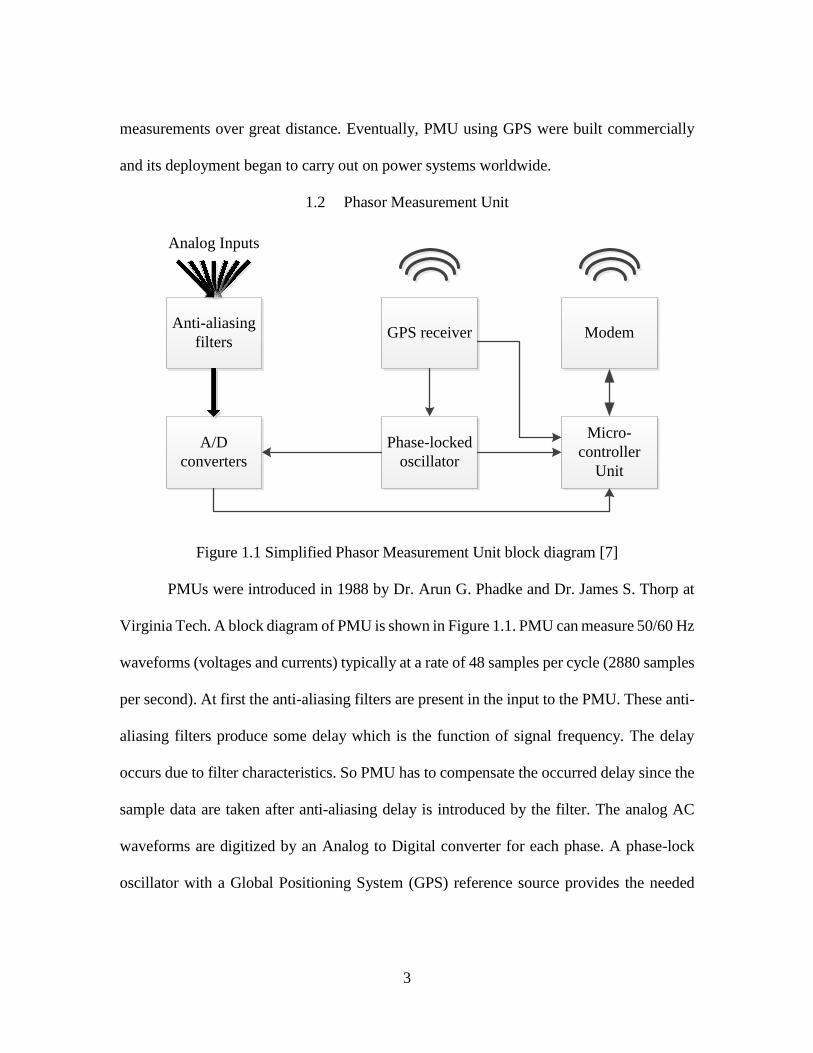
1.2 Phasor Measurement Unit

Anti-aliasing

filters

A/D

converters

Phase-locked

oscillator

Micro-

controller

Unit

ModemGPS receiver

Analog Inputs

Figure 1.1 Simplified Phasor Measurement Unit block diagram [7]

PMUs were introduced in 1988 by Dr. Arun G. Phadke and Dr. James S. Thorp at

Virginia Tech. A block diagram of PMU is shown in Figure 1.1. PMU can measure 50/60 Hz

waveforms (voltages and currents) typically at a rate of 48 samples per cycle (2880 samples

per second). At first the anti-aliasing filters are present in the input to the PMU. These anti-

aliasing filters produce some delay which is the function of signal frequency. The delay

occurs due to filter characteristics. So PMU has to compensate the occurred delay since the

sample data are taken after anti-aliasing delay is introduced by the filter. The analog AC

waveforms are digitized by an Analog to Digital converter for each phase. A phase-lock

oscillator with a Global Positioning System (GPS) reference source provides the needed

4

high-speed synchronized sampling with 1 microsecond accuracy. The captured phasors are

to be time-tagged based on the time of the UTC Time Reference.

Compared with traditional measurements received from Supervisory Control and

Data Acquisition (SCADA) system, these synchronized PMUs are hundred times faster in

capturing data and greater in measurement accuracy. SCADA systems are based on quasi-

steady state and therefore are not capable of measuring transient phenomena. SCADA

systems usually consists of Remote Terminal Units (RTUs) and are interfaced with sensors

that can measure only magnitude not the phasors. Integration of PMUs into the system

provides faster processing for state estimation due to the relationship between PMUs and

state variables. A power system is said to be observable if the measurements deployed on it

allows to determine the bus voltage magnitude and angle at every buses of the system. The

system observability can be estimated by considering the topology of the network, the types

and location of the measurements. Installing a PMU in a bus gives direct observability

because the phasor voltage of that bus is measured by PMU directly. Also knowing the fact

that PMU gives the current phasor of the branch or line which is interconnected to the bus

where PMU is installed. This feature of PMU typically makes the adjacent bus indirectly

observable because once the current phasors are available; voltage phasors can be estimated

or calculated using line parameters.

1.3 Literature Review on PMU placement

The primary goal of state estimator is to find the optimal estimates of bus voltage

phasors based on the available measurements in the system as well as the system network

topology. Generally, the measurements are provided by Remote Terminal Units (RTUs) at

5

the substation and include real/reactive power flows, power injections, magnitudes of bus

voltages and branch currents. Now, since commercial PMUs are widely available in the

market, some of the utilities or power industries have started deploying in their network,

whereas many of them intend to install in the grid/system in near future. At the end, the

most concerned question lies in the cost. As the cost of PMUs and their installation are

relatively very high, planning engineers are facing problem on planning the best location

for PMUs’ placement. Planning can either be for initial stage or for additional new PMUs

where the system network already contains some sets of PMUs.

As discussed in earlier section, observability of a system highly depends on number

of installed PMUs. If there is an occurrence of any unexpected outage in a system or in a

PMU itself, it will affect the system observability and may cause a serious problem [8-10].

Due to the critical nature of power systems, complete observability of all nodes at all times

is required.

The PMUs placement in strategic locations has been the vital research topic for PMU

application. Even though there are numerous applications of PMUs, this research and

discussion on PMU placement are strictly limited to state estimation application only. Power

engineers have introduced various methodologies all across the world [11]. The researchers

have approached the PMUs placement problem using two methods: (i) Heuristic approach

(ii) Mathematical approach.

1.3.1 Heuristic approach

Heuristic approach has been widely adopted in this area. Simulated annealing is used

in [12] to find the placement location based on desired depth of unobservability. This thesis

6

discussed the impact of depth of unobservability on the number of PMUs and was based on

network topology. A similar approach which utilizes the stochastic models to capture

dynamic state estimation uncertainties was also introduced in [13]. A sensitivity constraint

optimal PMU placement is presented in [14] . Location for placement of PMUs were

identified based on the buses with higher sensitivity and buses with more outlets. The

simulated annealing algorithm is used in the model to get full system observability.

Reference [15] solves the PMU placement problem using recursive Tabu search. Though

the algorithm used for this approach give satisfactory results for larger bus systems but no

robust contingency is considered. A new parallel Tabu search method for solving PMU

placement problem was presented in [16]. The model used in this literature has considered

the system with and without communication constraint. However the developed process

execution time is high even for lesser bus systems. An optimal deployment of PMUs using

differential evolution concept was presented in [17] for normal operating condition.

Literature [18] addresses on N-1 PMU failure and solves the PMU placement problem using

the same differential evolution process. Genetic algorithm in [19] solves the PMU

optimization problem with an objective to get full system observability with higher

measurement redundancy. Immunity genetic algorithm is proposed in [20]. The approach

used in [20] is relatively time consuming and is not preferable for large systems. Binary

Particle Swam Optimization (PSO) is another optimization approach that is enormously

used in this field. In [21], a simple PMU placement has been implemented using BPSO but

the algorithm does not consider details regarding PMU vulnerability. Since all the

7

techniques discussed in heuristic approach, being iterative in nature, requires time for

convergence and also the convergence fully depends on the initial guess.

1.3.2 Mathematical approach.

Mathematical approach has been gaining popularity from recent years. They are

easy to apply in the situation where a definite solution is required. They are based on

formulas derived from mathematical calculations. Integer linear programming is a common

approach as presented in [22], in which a general formulation for PMU placement using

conventional and without conventional measurement is taken into consideration.

Conventional measurements refers to zero injection measurements and branch flow

measurements. Using a similar concept, a unified approach is presented in [23] using binary

integer linear programming. The mathematical formulation described in this literature

considers the single PMU losses using zero injection and flow measurements separately.

Contingency constrained optimal PMU placement using exhaustive search approach is

proposed in [24]. This literature has taken several zero-injection buses in account for PMU

placement considering single PMU loss and measurement channel limitation. Mixed Integer

Linear Programming is used in [25] which considers zero injection and branch flow

measurements in order to maximize the measurement redundancy and reduce the number

of PMUs. However, the approach in [25] requires almost twice the amount of PMUs to

obtain full system observability under contingency operation than at normal operating

conditions.

8

1.4 Scope of the work and Objectives

To the best of my knowledge, all the literatures on PMU placement approaches

mentioned so far is limited to single PMU loss. However, PMU placement based on

vulnerability analysis is scant. Vulnerability can arise from various aspects like equipment

failure. Although PMUs are highly accurate enough to provide reliable data, there is an

unavailable possibility of PMU which may be caused by communication failures or line

outages. Furthermore, the networked PMUs might be rendered out of service by natural

disasters such as hurricanes or PMUs can be intentionally taken down by malicious attacks.

PMUs are also prone to cyber-attack. Since PMUs rely on GPS signal, there is a threat to

GPS spoofing which gradually result in false reading or loss of measurements [26]. Such

practical scenarios are likely to occur which are vulnerable to PMUs. Therefore while

placing the PMUs in the system for state estimation; its vulnerability should also be

accounted to study its impact on system observability. Hence, our objective of work is to

propose PMU placement approach considering vulnerability analysis.

The objective of this research work are as follows:

1. Deploying a fixed number of PMUs in the system considering the vulnerability of

PMU, in absence of conventional measurements.

2. Deploying a fixed number of PMUs in the system considering the vulnerability of

PMU, in presence of conventional measurements like zero injection and branch flow

measurements.

3. A strategy for placing additional PMUs in the system considering the resiliency of

measurement systems.

9

1.5 Outline of Thesis

This thesis is composed of five chapters. Chapter 1 gives a background on PMU,

their features and their importance in state estimation. Apart from that, literature reviews on

PMU placement methodologies and the objectives are also presented. A detail explanation

of the model used in PMU deployment approach considering with and without conventional

measurements is presented in Chapter 2. Their differences are elaborated with simple

examples. PMU placement considering its potential loss is also presented in chapter 3. The

influence of considering conventional measurements is also discussed. A flow chart with

consecutive steps for describing the approach is well presented. Cases study and results

obtained from the approach are also discussed. Chapter 4 explains the need to select critical

buses and the reason for prioritizing such buses when planning for PMU deployment. A

strategy for placing additional PMUs in the system with pre-existing PMUs is formulated

and the effectiveness of the approach is testified on IEEE test systems. Finally chapter 5

summaries the work and presents the recommendation for future research.

10

CHAPTER TWO

INTEGER LINEAR PROGRAMMING FORMULATION FOR OPTIMAL PMU

PLACEMENT

Over the last 10 years, Integer Linear Programming (ILP) or Integer programming

(IP) has been gaining a practical interest in variety of applications like planning, scheduling,

telecommunication network and more. This could possibly because of the enormous grown

in fast computing and improved algorithm. It is said that Integer Programming is the

foundation for much of analytical decision-making problems [27]. It contains three main

bodies: variables, constraints and objective function. Variables are the decision makers with

integer values, constraints are used to restrict the values to a feasible region. In Integer

Programming formulation, constraints must always be linear. It can be linear equality or

linear inequality or both. Objective function then defines whether to maximize or minimize

to get the optimal solution, depending upon the problem. The objective function should also

be linear in nature.

Using ILP for finding optimal PMU placement is currently on trend since it saves

the CPU computation time so greatly. This thesis work is done using Binary Integer

Programming (BIP). The difference between LIP and BIP is that the decision variables are

binary values (0, 1) in BIP. This chapter will give a review of general ILP formulation for

optimal PMU placement and is derived from [22]. The mathematical formulation will be

categorized into two different approaches: (i) Without conventional measurement (ii) With

conventional measurement.

11

2.1 Without Conventional Measurement

The approach in this section is applicable where the conventional measurements like

branch flow or any injection measurements are not considered.

2.1.1 Mathematical FormulationThe basic PMU placement problem for full

observability is formulated as follows:

N

k

kCxMin1

(2.1.1)

Subject to

PMUBAX (2.1.2)

N

C

1

111 (2.1.3)

T21 Nxxx X (2.1.4)

1,0kx

where

xk binary decision variable for PMU location;

otherwise0

busat present is PMU if1 kxk (2.1.5)

C the cost function

N number of bus nodes of the system.

A bus connectivity matrix for N bus system and is defined as

12

(2.1.6)

BPMU matrix with N×1 column vector whose entities are all ones.

The objective function in (2.1.1) defines the minimum PMU required to get full

system observability. Since the cost function for all PMUs is unity, it means the cost for

each PMUs are assumed to be equal. Inequality constraint (2.1.2) defines each bus in the

system should be observed at least by one PMU. The matrix A is the system admittance

matrix, which is transformed into binary form. This constraint guarantees the full

observability. The number of required constraints is N×N. The solution of this optimization

problem gives the minimum optimal number of PMUs and their corresponding locations.

Bus 7

Bus 3 Bus 4 Bus 5Bus 1 Bus 2

Bus 6

PMU

Figure 2.1 Seven bus system

otherwise0

or ajacent are and bus if1,

jijiA ji

13

2.1.2 Example Illustration

To illustrate the above problem, a seven bus system is used as shown in Figure 2.1.

The connectivity matrix in binary form is:

1000010

0100010

0011000

0011100

0001110

1100111

0000011

A

Now multiplying the connectivity matrix with the decision variables, for each bus

the constraints are as follows:

1

1

1

1

1

1

1

727

626

545

54314

4323

763212

211

xxA

xxA

xxA

xxxA

xxxA

xxxxxA

xxA

Ai

X

X

X

X

X

X

X

X

The operator sign “+” serves as logical “OR” and all the ones at the right hand side

of inequality constraint is the observability constraint. This means at least one variable of

each row containing summation the variables must be one or greater. For example, the very

first row indicates the bus 1 and according to constraint, PMU should be placed either at

bus 1 or bus2 to make bus 1 observable. Similarly the PMU should be placed either at bus

1, 2, 3, 6, or bus 7 in order to make bus 2 observable and so on. The resultant optimal number

14

of PMU for this system is two and the optimal locations are at bus 2 and bus 4. Hence the

placement gives full observability of the buses.

2.2 With Conventional Measurement

The most economical way of reducing the number of optimal PMUs to place in the

system is to consider conventional measurements. As mentioned earlier, conventional

measurements in this thesis refers to measurements like zero-injection and branch flow

measurements. Branch flow measurements are measurements between any two buses and

are already available in practical existing systems. Such measurements are already there in

the systems and the installation cost for branch measurements are very less compared to

PMUs. Using branch flow measurement voltage angle of any one bus can be determined.

Zero injection measurements are found in zero-injection buses. Any bus which does not

have generation or load is considered as zero-injection nodes. These zero-injection buses

need no metering and considered as accurate measurement for state estimation. They are

also regarded as pseudo measurements. When the system contains zero-injection buses there

are some rules associated with system observability [28].

i. The first rule implies: in zero-injection cluster (all the buses adjacent to zero-injection

bus and itself), if the zero-injection bus is observable and its adjacent buses are all

observable except one bus then the non-observable bus will eventually become

observable by applying KCL equation at zero-injection bus.

ii. The second rule is: within the zero-injection cluster if all the buses are observable

except the zero-injection bus, then that particular zero-injection bus can be identified

as observable by using nodal equations.

15

Combining these two rules simplifies that a zero-injection cluster is observable when

it has at most one unobservable bus.

An Observability Model

The observability model considers a sample six bus system as shown in Figure. 2.2

to explain the relationship between the PMUs and conventional measurements based on bus

observability. To illustrate the model let us define a vector G = AX. The element gi = Ai,j

xi of G indicates the measurement redundancy. Measurement redundancy means the

number of bus i is reached by a PMU. X is the PMU placement column matrix and xi is the

ith element of X and also regarded as decision variable; A is the bus connectivity matrix

and Ai,j is the ith row, jth column of A. The representation of matrix A and decision variable

matrix X is same as defined in earlier section 2.1.

Bus l

Bus jBus h Bus i

Bus k

Bus m

Branch flow

Zero

injection

Figure 2.2 A sample system

16

To demonstrate the resultant observability criteria to be fulfilled due to the presence

of conventional measurement, following three cases need to be analyzed.

i. Branch Flow Measurement. As seen from Figure 2.2, either bus i or j can be made

observable by this measurement whereas, the other bus must be observed by the PMU.

1≥ji gg (2.2.1.1)

ii. Zero-injection Measurement. Considering the zero injection measurement rules as

mentioned earlier, out of five buses in zero-injection cluster, minimum four buses

should be observed by PMU.

4≥lkjih ggggg (2.2.1.2)

iii. Hybrid Measurement. Combination of branch flow measurement and zero-injection

measurement is referred in this paper as hybrid measurement (bus i as shown in Figure

2.2). Excluding the conventional measurement buses, the remaining buses except one

bus in the zero-injection cluster should be observed by PMU. That one bus takes the

merit of hybrid measurement so it can be made observable.

2≥lkh ggg (2.2.1.3)

The right hand side of the equation (2.2.1.1-2.2.1.3) indicates the number of buses

that should be observed by PMU itself.

Mathematical Formulation

From the observability model in section 2.2.1, it is obvious that the system with

presence of conventional measurement can be categorized into two different types of buses;

the bus associated with conventional measurement and the bus which is not associated with

any conventional measurements. Therefore while formulating the constraint for optimal

17

PMU placement, the categorized buses should be kept in an order such that the bus not

associated with conventional measurement is in first order, then the buses with associated

conventional measurement is placed.

Now, the mathematical formulation when considering conventional measurement is given

below:

N

k

kCxMin1

(2.2.2.1)

Subject to

concon bAXPTPG

)()(

0

0

meas

MM

T

I (2.2.2.2)

where Tmeas and bcon are summation of buses associated with conventional measurements

and a constant number for those buses’ observability respectively. These are interpreted

same as described in above three cases; mentioned in section 2.2.1. M is the number of buses

not associated with conventional measurements and P is a permutation matrix.

Example Illustration

Let us consider a seven bus system considering a zero injection measurement and a

branch flow measurement. In the Figure.2.3, bus 2 is zero injection bus and branch flow

measurement is in between bus 2 and bus 3. According to above formulation, we have,

18

Bus 7

Bus 3 Bus 4 Bus 5Bus 1 Bus 2

Bus 6

Branch flow

Zero injection

PMU

Figure 2.3 A sample system with conventional measurements

1000010

0100010

0011000

0011100

0001110

1100111

0000011

A

Bus 4 and 5 are not associated to these two conventional measurements. The two

equality constraints corresponding to two conventional measurements are 132 gg and

2761 ggg .

2 meas.Injection

3-2 meas.Branch

11001

00110

measT

Each column in Tmeas refers to buses 1, 2, 3, 6, 7 respectively.

19

1100100

0011000

0000010

0000001

conT ,

1000000

0100000

0000100

0000010

0000001

0010000

0001000

P ,

2

1

1

1

1130011

0000221

1111001

0011000

7

6

5

4

3

2

1

x

x

x

x

x

x

x

XAPTcon

The resultant optimal number of PMU is two and the strategic location of PMU is

at bus 2 and bus 5. This example shows that conventional measurements are utilized in

PMU placement. Since a very small system was taken into consideration, the optimal

number of PMU considering with and without conventional measurement turned out to be

equal. However the placement location is different. The efficiency of this model is

significant for larger bus systems which will be discussed in next chapter.

20

CHAPTER THREE

PMU DEPLOYMENT APPROACH FOR MAXIMUM OBSERVABILITY

CONSIDERING ITS POTENTIAL LOSS

This chapter deals with the PMU placement approach which is implemented to get

maximum buses observability by addressing the PMU vulnerability. It is determined by

analyzing the PMU loss and their impact on system bus observability. In order to implement

this method, it requires more number of PMUs than normal operating condition. Since

PMUs are expensive, the approach is equally flexible even for increasing the PMU

requirement to just one additional than what is required for normal operating condition for

each tested systems. Unlike the above discussed literatures mentioned in chapter one,

possible loss of each PMUs that were supposed to be installed in the system are taken into

consideration. Loss of each PMUs are evaluated periodically in a way that only one PMU

loss is taken into consideration in each period. This is because the probability of single PMU

loss is more than the two PMU losses. The optimization model is further divided into two

parts. This chapter first explains the methodology without using conventional measurement

and secondly analyzes using conventional measurements.

3.1 Optimization Model without Conventional Measurement

3.1.1 Mathematical Formulation

The PMU deployment optimization problem proposed in this part is used to analyze

the vulnerability of PMU. This problem consists of two parts. The first is the increasing of

the NPMUs by one as illustrated in Figure 3.1. NPMUs refers to the optimal number of PMUs

required in the system to get full observability as discussed in chapter two. Then consider

the loss of (NPMUs +1) one at a time and solve the problem in (3.1.1.1) to (3.1.1.4). The main

21

objective of this problem is to locate the available number of PMUs in such a way

observable buses is satisfied.

) ( 1

'

1

n

Ni

i

N

i

i xxMax (3.1.1.1)

Subject to

BXA (3.1.1.2)

iiiii PxbPx max,

''

min,

' (3.1.1.3)

mX (3.1.1.4)

TNi xxxx 21X (3.1.1.5)

where

ix decision variable for PMU placement as described in chapter two,

'

ix binary decision variable which represents the buses observed by PMUs only,

N number of buses in the system,

n number of nonzero elements of connectivity matrix A ,

A bus connectivity matrix as represented in chapter two,

B observability constraint, column vector with all ones

121

nnbbb B

Pmin,i minimum number of nonzero elements of ith bus, which is chosen as 1,

Pmax,i total number of nonzero elements of connectivity matrix A corresponding to ith bus,

b'i the product of A and X after removing one of the PMUs,

22

m the number PMUs available for the system which is greater than the requirement for

normal operating condition.

Equation (5) implies

0if1

0 if0'

'

i

'

i

i b

bx (3.1.1.6)

PMUs from basic

placement from chapter

two using equations

(2.1.1) - (2.1.4)

Additional PMU

Apply proposed PMU

deployment using equations

(3.1.1.1) - (3.1.1.4)

Figure 3.1 Relationship of optimization under normal condition and proposed model

Before the description of above formulation, it is important to understand the term

“measurement redundancy”. Theoretically, “Measurement redundancy” of a bus means the

number of times the bus is being observed by PMUs. In practice, measurement redundancy

of each bus can be determined from the product of matrix A and X. Likewise, the system’s

measurement redundancy can be calculated by summing the measurement redundancy of

each buses.

This model tries to place the PMUs in such a way that the system’s measurement

redundancy is increased. The objective function (3.1.1.1) gives the location of available

number of PMUs and the maximum number of non-zero elements of A matrix that are

particularly being observed by PMUs respectively. The inequality constraint (3.1.1.2)

indicates that each buses should be observed by at least one PMU. Another inequality

23

constraints in (3.1.1.3) is an important and necessary condition to judge the strategic

location of PMU such that the measurement redundancy of the system is maximized even

when there is a single loss of PMU. The equality constraint in (3.1.1.4) denotes the number

of PMUs to be deployed in the system.

3.1.2 Deployment Approach

The flowchart for the proposed method is shown in Figure. 3.2. The algorithm is

described in following steps.

Step 1: Calculate the bus connectivity matrix A of the bus system in terms of binary

elements (1 and 0).

Step 2: Set the available number of PMUs m to be deployed in the system

Step 3: Optimize the PMU location considering constraints (3.1.1.2) and (3.1.1.4) as the

only constraint from section 3.1.1.

Step 4: Once the PMU locations are globally optimized, remove one of the installed PMUs

from the system to analyze the vulnerability. This process is carried out by removing

ith column from connectivity matrix which is equivalent to removing a PMU at ith

bus. Follow the objective function and all the constraint presented in equation

(3.1.1.1)-(3.1.1.4) from section III.

Step 5: After the optimization, the number of observed nodes (covered by PMUs) are

obtained. Repeat step 4 for other remaining PMUs. In this proposed model only one

PMU is removed at a time.

Step 6: Evaluate whether the inequality constraint (3.1.1.3) is satisfied or not to indicate the

maximum observability.

24

Step 7: If maximum observability is obtained this ends the process. Else update the PMU

location again and follow steps 4 to 6 until the program terminates with optimal

result.

When analyzing the effect of removing a PMU from a bus i, only the buses that are

connected to it are assessed instead of all the buses. In doing so, the number of variables

and constraint equations are reduced by an enormous amount especially, when the size of

the system is large. Essentially, the numbers of additional variables are N + n and number

of additional constraint equations is N + 2n.

Initilization

Step 1: Build A

matrix

Step 2: Set m

Step 3: Optimize the PMU

location using proposed

model

Step 7: Update the PMU

location

i = i + 1

Step 4: Assume a

potential loss of a PMU

and obtain B'

Step 5: i < n

Step 6: Maximum bus observed ?

End

Yes

No

No

Yes

Strategical

deployment scheme

PMU 1

PMU 2

PMU i

PMU n

Figure 3.2 Flow chart of proposed algorithm

3.1.3 Case Study

The proposed method is tested on the IEEE 14, 30, 57, 118 and 300 bus test systems

[29]. The single line diagram of the test systems can be obtained from [29, 30]. The

25

optimization is executed in Matlab environment using the binary linear programming

toolbox.

3.1.3.1 PMU Placement Locations

The optimal number of PMUs (NPMUs) and the corresponding locations are shown

in the second and third columns of Table 3.1, respectively. Whereas the PMU deployment

for maximizing the number of observable buses (measurable buses by PMUs) is

summarized in columns four and five of Table 3.1. The resultant PMU locations for IEEE

14-bus system are buses 2, 6, 7, 9 and 14. In this particular system, all the PMU locations

are same as that of basic placement case (under normal operation). The extra PMU is located

at bus 14. Though it seems that the optimization is carried out locally but it is not.

Coincidently it happens to be optimal locations. In 57-bus system, only 6 buses are

commonly placed by both of them. For larger systems like 118 and 300 bus systems, large

number of PMUs is identically placed.

3.1.3.2 Effect on System Observability

The optimization problem tested in this work assumes the criticality of each PMU.

It is not known earlier that which PMU measurement will be lost. Therefore, each installed

PMU is assumed to have equal possibility of unavailability.Table 3.2 shows the detailed

observability study of the 14-bus system. In this Table, the number of PMUs is 5 in total

and the unobservable buses (while considering loss of each of the single assigned PMU) are

presented. As expected from the proposed approach, small number of buses is unobserved.

The redundancies of the respective buses are also shown for the system. As it can be seen

26

Table 3.1 PMU installed location for the test systems

Test

system

Basic PMU placement Proposed PMU deployment

Optimal

no. of

PMUs

(NPMUs)

Optimal PMU locations

at buses m PMU location at buses

14 bus 4 2 6 7 9 5 2 6 7 9 14

30 bus 10

1 7 9 10 12 18 24

25 27 28

11

1 7 10 11 12 19 24 25

27 28 29

57 bus 17

1 2 6 13 19 22 25

27 29 32 36 39 41

45 47 51 54

18

1 6 9 15 19 22 24 28

31 32 35 38 41 47 50 53

56 57

118 bus 32

3 7 9 11 12 17

21 25 28 34 37 41

45 49 53 56 62 63

68 70 71 76 79 85

86 89 92 96 100 105

110 114

33

3 5 10 11 12 17 21

25 28 34 37 40 45 49

53 56 62 63 68 70 71

77 80 85 86 90 92 96

100 105 110 114 118

300 bus 87

1 2 3 11 12 15

17 22 23 25 26 27

33 37 38 43 48 49

53 54 55 58 59 60

62 64 65 68 71 73

79 83 85 86 88 92

93 98 99 101 109 111

112 113 116 118 119

128 132 135 138 139

143 145 152 157 163

167 173 183 187 188

189 190 193 196 202

204 208 210 211 213

216 217 219 222 226

228 267 268 269 270

272 273 274 276 294

88

1 2 3 11 12 15 20

22 23 25 27 33 37 38

43 48 49 53 54 55 58

59 62 64 68 69 71 73

79 83 85 86 88 89 93

98 99 101 103 109 111

112 113 116 118 119 122

132 133 138 143 145 152

157 160 163 173 177 183

187 189 190 193 196 200

204 208 210 211 213 216

217 219 222 224 228 238

252 267 268 269 270 272

273 274 276 294 300

27

from Table 3.2, with the PMU at bus 14 is lost, the system still manage to get full

observability. Tables 3.3, 3.4 and 3.5 summarizes the observability of the IEEE 30, 57 and

118 bus systems respectively. The redundancy of each bus is not shown but the numbers of

buses which are observed by more than one PMU are clearly mentioned.

Table 3.2 Observability results for the IEEE 14 bus system

When PMU at bus 2 is lost

Buses 1 2 3 4 5 6 7 8 9 10 11 12 13 14

Redundancy of

each bus 0 0 0 2 1 1 2 1 3 1 1 1 2 2

Unobservable

buses 1,2,3


Buses 1 2 3 4 5 6 7 8 9 10 11 12 13 14

Redundancy of

each bus 1 1 1 3 1 0 2 1 3 1 0 0 1 2

Unobservable

buses 6,11,12


Buses 1 2 3 4 5 6 7 8 9 10 11 12 13 14

Redundancy of

each bus 1 1 1 2 2 1 1 0 2 1 1 1 2 2

Unobservable

buses 8


Buses 1 2 3 4 5 6 7 8 9 10 11 12 13 14

Redundancy of

each bus 1 1 1 2 2 1 1 1 2 0 1 1 2 1

Unobservable

buses 10


Buses 1 2 3 4 5 6 7 8 9 10 11 12 13 14

Redundancy of

each bus 1 1 1 3 2 1 2 1 2 1 1 1 1 1

Unobservable

buses null

28


Lost PMUs 1 7 10 11 12

Unobservable

buses 1,2,3 5,7 10,17,21 11 4,12,13,14,15,16

Number of buses

observed by more than

one PMU

10 10 7 9 10

Lost PMUs 19 24 25 27 28 29

Unobservable

buses 18,19 23 26 null 8 null

Number of buses

observed by more than

one PMU

8 9 9 7 9 8


Lost PMUs 1 6 9 15 19 22

Unobservable

buses 2,16,17 4,5,6,7 9,10,12,55 3,14,45 18,19,20 21

Number of buses

observed by more

than one PMU

15 16 14 14 17 14

Lost PMUs 24 28 31 32 35 38

Unobservable

buses 24,25,26 27,28,29 30 33 35,36 37,44

Number of buses

observed by more

than one PMU

16 17 15 14 16 13

Lost PMUs 41 47 50 53 56 57

Unobservable

buses 43 46,47 50,51 52,53,54 40 39

Number of buses

observed by more

than one PMU

14 16 16 17 14 16

29


Lost PMUs 3 5 10 11 12 17

Unobservable

buses 1 6,8 9,10 14

2,7,14,

117

15,17,18,30,

31,113

No. of

redundant

buses

40 39 40 38 39 39

Lost PMUs 21 25 28 34 37 40

Unobservable

buses 20,21,22 23,25,26 28,29

19,36,4

3

33,35,3

8 41

No. of

redundant

buses

40 39 39 39 36 37

Lost PMUs 45 49 53 56 62

Unobservable

buses 44,46 47,48,50,51 52,53

55,56,5

7,58 60,61,62,67

No. of

redundant

buses

38 36 40 39 39

Lost PMUs 63 68 70 71 77 80

Unobservable

buses 63,64 65,68,116 24,74 72,73 78 79

No. of

redundant

buses

39 39 38 38 37 34

Lost PMUs 85 86 90 92 96 100

Unobservable

buses 83,84,88 87 90 93,102 95 101

No. of

redundant

buses

38 38 39 37 37 34

Lost PMUs 105 110 114 118

Unobservable

buses

105,107,

108

109,110,11

1,112

32,114,

115 118 _

No. of

redundant

buses

38 40 40 39 _

30

From these Tables, it can be noticed that the impact of PMU loss on the observability

is more for the larger systems. Some of the PMUs are very critical, therefore losing those

particular PMUs will result in greater number of unobservable buses. The most critical PMU

for 118 bus system is at bus 17. When the PMU placed at bus 17 is lost, almost 6 buses

become unobservable. Apart from that, the implemented algorithm locates the available

PMUs in such a way that the maximum number of observable buses are obtained when any

of single PMU is unavailable. For the 300 test system, the large number of uncovered buses

is 8 which corresponding to missing the PMU at bus 268. This system is found fully

observable if the PMU at bus 300 lost.

3.2 Optimization Model with Conventional Measurement

In this section, we will only discuss the mathematical formulation and the simulated

results because all other approaches are same as that of model discussed in section 3.1. The

only difference lies is the consideration of conventional measurements.

3.2.1 Mathematical formulation

The objective of PMU placement problem is to analyze the vulnerability of PMUs

by deploying a limited number of PMUs m corresponding to the cost associated with it. For

simplicity, the cost for all the PMUs is assumed as unity and all the PMUs have sufficient

channels to observe adjacent buses’ current phasors.

Mathematically,

) ( 1

'

1

n

Ni

i

N

i

ii xxcMax (3.2.1.1)

Subject to

31

concon bAXPT )( (3.2.1.2)

iiiiconi Pxbbx max,

''

,

' (3.2.1.3)

mX (3.2.1.4)

TNi xxxx 21X (3.2.1.5)

where,

c is the cost function defined by row matrix containing all ones as N1

111 .

Remaining all other matrix vectors, variables are described earlier in section 3.1 and

2.2.2 (chapter two). The only difference between in the above formulation between the

proposed placement techniques considering conventional measurement and without

conventional measurement is constraint (3.2.1.2) and (3.2.1.3). The detail explanation for

(3.2.1.2) was already discussed in chapter two. When compared to mathematical

formulation used in section 3.1 of this chapter when considering system without

conventional measurement and here is that the observability constraint or all buses are not

same or unity. Due to advantage of zero injection and flow measurement, it is not necessary

that each of the buses should be observed by at least a PMU. Depending upon the buses

associated with and without zero injection and flow measurement, the value of observability

constraint for some buses can be 0 or 1 or 2 or so on.

3.2.2 Case Study

The proposed method is tested on IEEE test system buses 14, 30,118 and 2383

western polish. The single line diagram of test systems can be obtained from [29]. The

measurement bus specification of conventional measurements are shown in Table 3.6 for

32

all four test systems. Two different cases has been designed to analyze the result. Case A is

for PMU placement without using conventional measurement and case B is for placement

based on conventional measurements. Information given in Table 3.6 is designated only for

case B. For the system with 2383 bus system, the location of zero injection is shown in

appendix A.

Table 3.6 Test system specifications

IEEE Test System 14 30 118 2383

No. of Zero-injection Buses 1 6 10 552

Location of Zero-injection Buses

7 6, 9, 22,

25, 27, 28

5, 9, 30, 37, 38, 63, 64, 68, 71, 81

¯

Number of Branch Flow Measurement

2 1 1 1

Branch Flow

Measurement

Buses

From 6 7 2 15 8

To 12 8 6 33 18

Table 3.7 Comparisons of PMU deployment schemes in two cases

Test System

Case A Case B

Nmin m PMU Locations Nmin m PMU Locations

IEEE bus 14

4 5 2, 6, 7, 9, 14 3 4 2, 4, 6, 9

IEEE bus 30

10 11 1, 7, 10, 11, 12, 19, 24, 25, 27, 28, 29

7 8 1, 7, 10, 12, 19, 24, 27, 28

IEEE bus 118

32 33

3, 5, 10, 11, 12, 17,

21, 25, 28, 34, 37, 40,

45, 49, 53, 56, 62,

63, 68, 70, 71, 77,

80, 85, 86, 90, 92, 96,

100, 105, 110,114,

118

28 29

3, 9, 12, 15, 19, 22, 27, 31, 32, 34, 42, 45, 49, 53, 56, 62, 65, 70, 75, 79, 85, 86, 90, 92, 96, 100, 105, 110, 118

2383 polish

746 747 ¯ 561 562 ¯

33

3.2.3.1 PMU Placement Locations

The optimal number of PMU for the full observability of the test system, under

normal operating conditions (Nmin) is achieved. Depending upon that, an additional PMU is

made available to deploy into the system. All the total number (m) PMUs globally optimized

and are placed at specific locations as shown in Table 3.7. In order to maintain the

measurement accuracy, the number of PMUs is considered to be greater than or equal to

conventional measurements. Since conventional measurements are used in case B, the

requirement for number of PMUs is decreased by enormous amount. Comparing the PMU

placement location between two cases, it can be inferred that the maximum number of buses

happens be to commonly placed. As seen for 14 bus system, in case A, there are 5 PMUs

and out of them, the location chosen for almost three PMUs i.e. 2, 6 and 9 are at the same

location in case B, as in case A. The common location is seen more as the system buses

increases or for the large system like 118 bus system and 2383 bus system. For 2383 polish

system, the PMU locations are shown in appendix A.

While proposing optimization process, no constraint was imposed such that the

PMU will not be placed at zero injection buses. Due to this obvious reason, proposed

optimized method results in deploying PMU even at zero-injection buses. For example, in

IEEE 30 bus system, bus-27 is referred as zero-injection bus and one of the optimal location

of PMU is bus-27 itself.

3.2.3.2 Effect of System Observability

The optimization problem tested in this work assumes the criticality of each PMU.

It is not known earlier that which PMU measurement will be lost. Therefore, each installed

34

PMU is assumed to have equal possibility of unavailability. The result shown in Table 3.7

does not guarantee to give full observability of the system. Figure 3.4 and Figure 3.5 shows

the detailed observability study of IEEE 14 and 30 bus test system respectively. Each of

those two figures illustrates measurement redundancy (Ai xi ) of ith bus when each of the

single PMU are lost. As it can be seen from the Fig. 3.4, when PMU at bus 4 is lost, all the

buses have redundancy of at least one except for bus 8. Since bus 7 is zero-injection bus

therefore using zero-injection rules, bus 8 can be made observable. Hence it can be said that

even if the PMU at bus 4 is lost, the remaining PMUs manage to give full observability of

the system. Such scenario might not be possible when other PMUs are out of service.

Figure 3.3 Measurement redundancy of IEEE 14 bus system

35

Figure 3.4 Measurement redundancy of IEEE 30 bus system

Nevertheless, the maximum number of buses will be observable. Figure 3.3 and 3.4,

also illustrates the criticality of the placed PMUs. To clarify further, from the redundancy

chart, it can be known that loosing which of the PMU results in greater number of

unobservable buses. For example for IEEE 30 bus system, the Figure 3.4 shows that when

PMU at bus 12 is unavailable, in total eight buses will be unobserved directly. PMU at bus

12 can be treated as critical one. The redundancy chart for remaining test system are not

shown here but can be easily obtained with the help of PMU placed location resulted in

Table 3.7.

36

3.3 Conclusion

This chapter discussed the PMU placement strategy with very limited amount of

PMUs to maximize the system observability. All the deployed PMUs were considered to

have an equal probability of failure. Therefore the obtained PMU location ensure that even

if any one of the PMU falls out, the remaining deployed PMUs still makes the maximum

buses observable. An additional maximum observability constraint was proposed. The

proposed method is also significant to analyze which of the PMUs is more critical. Binary

Integer Programming was used to obtain deterministic solution and the optimization was

rather done globally. This approach can be efficiently used to study the system observability

for random installation of the PMUs in sub-transmission system.

37

CHAPTER FOUR

A STRATEGY FOR PMU PLACEMENT CONSIDERING THE RESILIENCY OF

MEASUREMENT SYSTEM

This chapter presents an approach to find strategic locations for additional Phasor

Measurement Units (PMUs) installation while considering resiliency of existing PMU

measurement system. Due to the critical nature of power systems, complete observability

of all nodes at all times is required. However, the networked PMUs might be rendered out

of service by natural disasters such as hurricanes or PMUs can be intentionally taken down

by malicious attacks. Enough attention should be given to PMU vulnerability while placing

PMUs in the system. The concept of economically deploying PMUs considering resiliency

of existing system post attack is missing in the above literatures mentioned in chapter one.

Hence, this chapter highlights a considerable interest in improving PMU redundancy at

minimum cost. In order to ascertain a subset of nodes which are most likely to be attacked,

a virtual attack agent is modeled. The aim of the virtual attack agent is to reduce system

observability to a minimum while carrying out a coordinated attack on a subset of PMU

installation nodes. This virtual attack is used by the operator agent to identify a set of critical

nodes whose redundancy needs to be increased. The planner agent then finds strategic

locations to place additional PMUs in order to increase redundancy of critical nodes while

minimizing incurred cost.

Agent Based PMU Placement Framework

An uncertainty constraint PMU placement problem can be expressed in three

different agent based stages:

Attacker: A virtual attack agent is introduced whose goal is to take down a set of installed

38

PMUs to reduce system observability. Uncertain events like intentional attacks is an

important aspect that needs to be considered while making PMU placement decision. Due

to geographical span of interconnected power systems planning a coordinated attack on all

of the installed PMUs is improbable. Hence, the virtual attack agent will carry out

coordinated attacks on a subset of installed PMUs that are deemed critical. Here, the set of

critical PMUs are the ones when taken out of service minimizes system observability.

Cardinality of the critical set is assumed to vary depending on the resources available to

virtual attack agent.

Operator: At this stage, the operator has to take corrective measures to mitigate the

possible damage caused by the attacker. The operator agent identifies a set of critical nodes

based on virtual attack agents attack plan. The operator agent then relays the corrective

measure, which in this case is to increase the redundancy of critical nodes, to the planner

agent.

Planner: The task of planner is to deploy additional PMUs to increase redundancy of

critical nodes at minimum cost.

Schematic representation of the three cyclic stages is shown in Figure 4.1. The

schematic is cyclic in nature because of the nature of the problem, where the virtual attack

agent comes up with strategies to minimize system observability given a set of PMU

locations. The operator and planner agents then mitigate the effect of virtual attack agent by

placing additional PMUs at strategic locations. The virtual attack agent then starts a new

cycle with the new set of PMU installation locations.

39

Planner

OperatorAttacker

Planning

Scheme

PMU Outage

Corrective

Measure

Figure 4.1 Relationship between three agents in PMU placement

Each undesired PMU outage caused by the virtual attack agent is an optimization

scenario for the operator. These undesired outages can be single, double or multiple based

on virtual attack agent’s resources. Let P be the number of PMUs deployed into the system

and Ψ be the scenario which corresponds to the number of PMUs to be attacked by the

attacker. The total scenario can be represented as combinatorial number P CΨ as:

!-P !

!

PCP (4.1)

Since there are hundreds of thousands of possible attack scenarios, it is impossible

to enumerate all scenarios for large systems due to computational burden. Instead, by

adopting the approach in (4.2) a worst case scenario can be obtained.

% P (4.2)

where ƞ∈[0, 100] – representing the percentage of installed PMUs that are attacked. As a

worst-case scenario, an assumption has been made that the attacker can attack up to 50% of

the total deployed PMUs. Depending upon ƞ value, a set of attacked PMUs Ψ=[Ψ1,

Ψ2,…….,Ψz] is obtained from the optimization problem and this set is named as critical

40

PMUs. The programming framework for the agent based PMU placement is shown in

Figure 4.2.

Resources Available

η1 η2 η3 ... ηz

Ψ1 Ψ2 Ψ3 .. Ψz

Output from

Attacker plan

Input to

operator for

planning

Number of

Attacked

PMUs

Set of Attacked

PMUs

Most critical set of

PMUs

More weightage to the

buses with critical

PMUs

Figure 4.2 PMU placement Framework

41

Mathematical Formulation

Development of agent models as an optimization problem is discussed in this

section. The initial deployment locations for PMUs, which act as the starting point for the

proposed agent based framework are obtained using optimal PMU placement algorithm

from [22].

4.2.1 Virtual Attack Agent

The objective of virtual attack agent is to attack a subset of installed PMUs in the

system such that the system bus observability is minimized. The attack agent is modeled

using binary integer programming.

The mathematical formulations for attacker’s objective is as follows:

m

lk

k

1

min (4.2.1.1)

Subject to

iiki xAA (4.2.1.2)

z

l

p

xpx

)(1

(4.2.1.3)

1 ,0, 1 ,0 ipk xxand (4.2.1.4)

The objective function (4.2.1.1) ξk is the decision variable that tends to give the

observability of each bus in terms of binary variable. If the bus is observable by PMUs

remaining in the system after the coordinated attack by virtual attack agent then ξk will take

the value of 1 and if the bus is not observable by any of the PMUs then ξk will take the value

‘0’. In general, observability of a bus can be 0 in which case the bus is not observable or

42

observability can be a positive number which means the bus is observable.

otherwise0

0. if1 pi

i

xA (4.2.1.5)

Since the available PMUs were placed based on system network topology, it

becomes necessary to define a network connectivity matrix A.

Elements in matrix A are defined as follows:

otherwise0

adjacent are and or if1 jijiAij

(4.2.1.6)

In constraint (4.2.1.2), xi is an auxiliary binary variable of PMU placement. If the

PMU is present at the ith bus then xi is regarded as 1 otherwise 0. Before the attack, the

observability of the ith bus denoted by left-hand side of (4.2.1.2) should be equal to the

product of connectivity matrix of bus i and PMU placement variable xi. Since the attacker

already know the exact location of the PMUs, the attacker agent tries to enumerate all the

possibilities to destroy or damage the PMU which are critical. This procedure is presented

in (4.2.1.3). The word ‘critical’ defines those set of PMUs whose installation in the system

increases the system observability. Post attack the variable xi is zero for the disabled or

attacked PMU. In this case, the constraint (4.2.1.2) will act as inequality constraint because

the observability of the bus at left hand side will be greater than right hand side. The

connectivity matrix is always fixed as long as all the transmission lines in the system are in

service. The variable xp is the PMU placement variable post attack. Depending upon the

auxiliary variable xp, the attacker performs all combinatorial number and checks the

observability of each bus one by one. Those combination sets where the observability of

bus shows the maximum number, the attacker tries to attack on those particular sets of

43

PMUs. Constraint (4.2.1.2) helps the attacker to judge the most attractive set of PMUs to

act on.

Computational complexity of this optimization model increases substantially when

dealing with large number of system buses. From (4.2.1.2), the total number of inequality

constraints is equal to the number of system buses N and the equality constraint (4.2.1.3) is

split into two sections, one for the set of the buses where PMUs were installed and other for

the set of buses where PMUs were not installed. Therefore the total number of constraints

is N+1+1. Similarly the total numbers of variables are twice the number of system buses M.

This is because the first half M/2 denotes the auxiliary variable of PMU placement post

attack and the other half M/2 denotes the bus observability.

4.2.2 Operator Agent

The responsibility of the operator is to identify vulnerable nodes based on the

behavior of virtual attack agent. Vulnerable nodes in this context are a set of critical buses

whose observability is compromised by the virtual attack agent. Critical buses are the buses

include critical PMU installation buses and buses that are observable by critical PMUs.

The number of PMUs attacked by virtual attack agent is a percentage of the total

number of installed PMUs. Since, larger systems have larger number of installed PMUs, the

number of critical buses also tends to increase with system size. Since various sets of PMUs

were obtained depending upon the availability of attacker’s resources. Now, with the

concern of PMU’s and their installation cost, from those several sets of classified critical

PMUs, the planner has to choose only the most repeated PMUs among all sets of critical

PMUs. To obtain this, following formulation is used.

44

21R (4.2.1.1)

ZRS ...3 (4.2.2.2)

where S=[s1, s2,…, sw], denotes set of critical PMUs in (4.2.2.2).

The critical buses are those buses that are observable from the set of critical PMUs.

wi

B

c sAW (4.2.2.3)

B

fc

B

c

B

c

B

c wwwW , 2 , 1 , ,....,, (4.2.2.4)

where WcB is represented for set of critical buses obtained from each critical PMUs sw and

θ is the index of buses which are adjacent to critical PMU located buses.

4.2.3 Planner Agent

The objective of the planner agent is to install additional PMUs in strategic locations

to mitigate the vulnerability posed by virtual attack agent. The optimal PMU placement

considering the critical PMUs is as follows:

'

1

min i

N

i

i xc

(4.2.3.1)

iif,

B

ci bxwA '

)( (4.2.3.2)

'' )( iifc,

B

i bxwA (4.2.3.3)

N

i

ieq xXA1

' (4.2.3.4)

Nic

1111 (4.2.3.5)

1 ,0'

ix , Ni 2,..... 1, (4.2.3.6)

45

The objective function (4.2.3.1) implies that minimum number of PMU is placed in

the system and x'i is the new decision variable for PMU placement for this particular model.

It is defined same as xi as described earlier in attacker’s model. In this model, bi is

observability constraint for non-critical buses and is considered equivalent to one. Whereas

for critical buses, the observability constraint b'i is considered as two. Therefore constraints

(4.2.3.2) and (4.2.3.3) describes that each non-critical bus 𝑤𝑐𝐵 and critical buses 𝑤𝑐𝐵 must

be observable by at least one PMU and two PMUs respectively. Equality constraint (4.2.3.4)

represents that original PMUs has to be placed in the same location. Thus, under any

uncertain events or attacks, all the buses are still observable and with higher redundancy

with additional number of PMUs in the system. There are N number of variables and 2N

number of constraints. In this proposed model, the restrictions on number of additional

PMUs is not implemented. However, this optimization model has the potential to optimize

the fixed amount of additional PMUs just by adding a new constraint such that the

summation of decision variable is equal to a constant number.

Case study

The performance of proposed model is tested on 14, 30, 57 and 118 IEEE test bus

systems including large power system 2383 bus Western Polish system [29, 30]. All the

testified cases are implemented on 1.70 GHz processor with 6 GB of RAM using

CPLEX12.6.2 Solver. The optimization is executed in MATLAB environment.

4.3.1 Critical PMUs

The number of critical PMUs depends upon the size of the system and the system

topology. The set of PMUs that poses a higher influence in increasing the system bus

46

observability are shown in the Table 4.1. The critical PMUs are obtained based upon the

resources available to the attacker. The percentage shown in the Table 4.1indicates that the

attacker has ability to damage certain percentage of the total deployed PMUs in the system.

For a small system like 14 bus system, only 4 PMUs are needed in the system for full

observability before attack. 10% of 4 PMUs being a negligible number, 20% and 50% of

total placed PMUs is considered for execution. Nmin is the number of attacked PMUs.

Similarly, Table 4.1 demonstrates all the critical PMUs for different IEEE systems.

To further analyze strictly critical PMUs, only one set of PMUs per system is

evaluated. The PMUs that happens to be critical for more than twice among the

differentiated level of resources availability are only considered as most critical PMUs.

Figure 4.1 shows all such single set of most critical PMUs for 14, 30, 57 and 118 IEEE bus

systems only. The model was further tested for larger power systems like IEEE 300 and

2383 Western Polish system. For the larger system, the most critical PMU buses are shown

in Table 4.2. The critical PMUs for larger systems are selected based on 10% of total

installed PMUs. Since the numbers of PMUs installed in IEEE 300 and 2383 Western Polish

system outnumbered to smaller system, PMU installed buses are not shown in the described

Table 4.2.

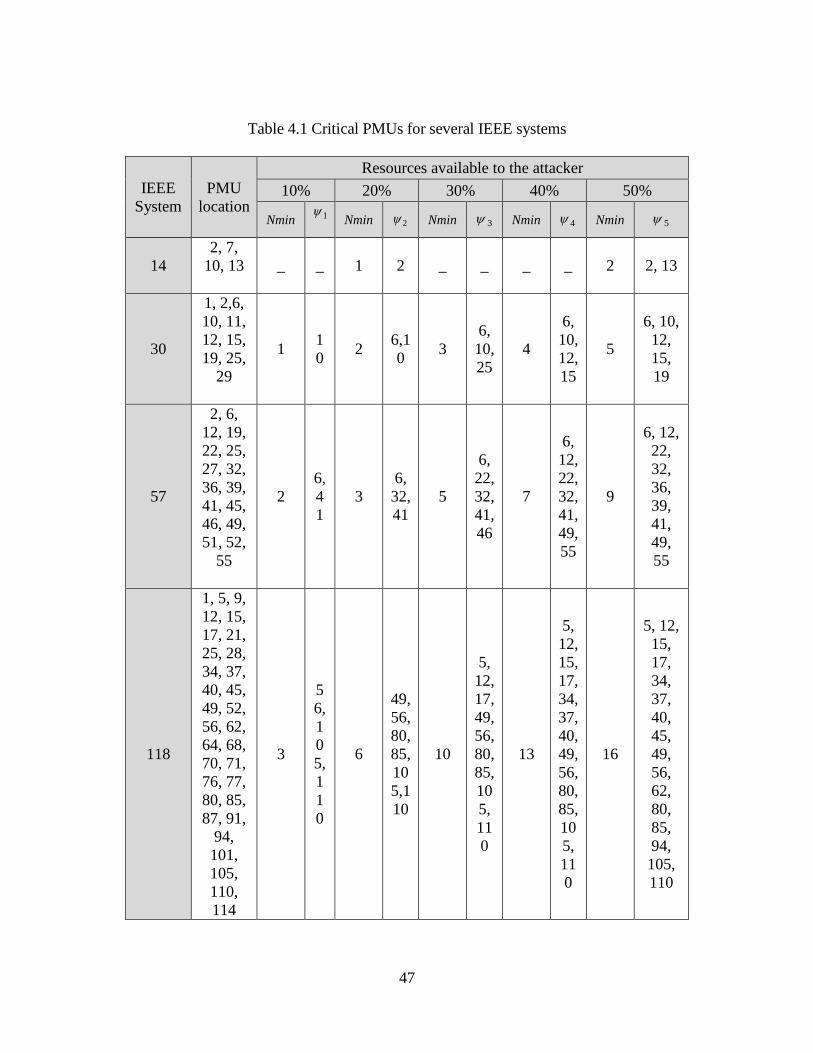
47

Table 4.1 Critical PMUs for several IEEE systems

IEEE

System

PMU

location

Resources available to the attacker

10% 20% 30% 40% 50%

Nmin 1

Nmin 2 Nmin 3 Nmin 4 Nmin 5

14

2, 7,

10, 13

_ _ 1 2 _ _ _ _ 2 2, 13

30

1, 2,6,

10, 11,

12, 15,

19, 25,

29

1 1

0 2

6,1

0 3

6,

10,

25

4

6,

10,

12,

15

5

6, 10,

12,

15,

19

57

2, 6,

12, 19,

22, 25,

27, 32,

36, 39,

41, 45,

46, 49,

51, 52,

55

2

6,

4

1

3

6,

32,

41

5

6,

22,

32,

41,

46

7

6,

12,

22,

32,

41,

49,

55

9

6, 12,

22,

32,

36,

39,

41,

49,

55

118

1, 5, 9,

12, 15,

17, 21,

25, 28,

34, 37,

40, 45,

49, 52,

56, 62,

64, 68,

70, 71,

76, 77,

80, 85,

87, 91,

94,

101,

105,

110,

114

3

5

6,

1

0

5,

1

1

0

6

49,

56,

80,

85,

10

5,1

10

10

5,

12,

17,

49,

56,

80,

85,

10

5,

11

0

13

5,

12,

15,

17,

34,

37,

40,

49,

56,

80,

85,

10

5,

11

0

16

5, 12,

15,

17,

34,

37,

40,

45,

49,

56,

62,

80,

85,

94,

105,

110

48

Figure 4.3 Critical PMUs in different test systems

Table 4.2 Critical buses with PMUs on larger systems

IEEE Test System

Total installed PMUs Selected critical PMU buses

300 bus system

87 3 15 109 112 190 268 269 270 272

2383 polish 746

6 18 29 133 246 309 310 321 322 353 354 361 365 366 374 425 456 494 511 525 526 527 546 556 613 644 645 679 694 717 750 754 755 796 797 870 923 944 978 979 1050 1096 1120 1138 1190 1201 1212 1213 1216 1217 1245 1483 1504 1524 1647 1664 1669 1680 1761 1822 1882 1883 1885 1919 1920 2112 2113 2166 2195 2196 2235 2258 2261 2274 2323

49

4.3.2 Planning Scheme for PMU Placement

The PMU placement planning scheme is presented in this section. The goal of the

planning scheme is to place additional PMUs in order to mitigate the loss of observability

in the event of an attack. From the previous section, the set of critical buses with respect to

loss of observability was obtained. The planner agent uses this information to obtain PMU

placement scheme for installing additional PMUs with least cost to increase redundancy of

critical nodes. For the most critical buses as shown in Table 4.3, the measurement

redundancy was set to 2 i.e. the most critical buses must be observable by at least 2 PMUs.

The resultant optimal numbers of PMUs are shown in Table 4.4. For IEEE 14 bus system,

two additional PMUs are required to increase redundancy of five critical buses. Similarly

for IEEE 30 bus system four additional PMUs are required to increase redundancy of 12

critical buses. Since the original PMU deployment was shown in Table 4.1, the following

Table 4.4 shows PMU locations only for additional PMUs. Due to space limitation, location

of additional PMUs for larger systems are not tabulated but are rather summarized as

follows. For IEEE 300 bus system, 30 additional PMUs are required. While the 2383 bus

polish system required 252 PMUs in addition to the originally placed 746 PMUs to obtain

full bus system observability and increased redundancy at critical buses.

50

Table 4.3 Critical buses for different test systems

IEEE Test System

Critical Buses

14 1 2 3 4 5

30 2 4 6 7 8 9 10 17 20 21 22 28

57 4 5 6 7 8 11 21 22 23 31 32 33 34 38 41

42 43 56

118

2 3 4 5 6 7 8 11 12 14 15 16 17 18 30 31 42 45 47 48 49 50 51 54 55 56 57 58 59 66 69 77 79 80 81 83 84 85 86 88 89 96 97 98 99 103

104 105 106 107 108 109 110 111 112 113 117

Table 4.4 Comparison of No. of optimal PMUs under normal and abnormal condition

IEEE

Test

System

No. of Optimal PMUs % of Additional

PMUs compared

with original

placement

Additional PMU Placement

Location considering critical

buses

Normal

Operating

Condition

More

weightage

to critical

PMUs

14 4 6 50% 1 4

30 10 14 40% 5 8 12 16 22

57 17 26 53% 4 7 11 21 23 30

33 34 42

118 32 51 59%

4 6 8 18 32 46

54 57 58 78 83 88

96 100 106 108 111

112 117

51

Conclusion

This chapter proposes a planning approach for optimal PMU placement making the

system more resilient to PMU failure. The likelihood of undesired events are analyzed by

creating a virtual attack agent which intends to damage some of the critical PMUs in the

system. Operator agent is used to obtain a subset of buses that are critical based on the attack

pattern of virtual attack agent. Simulation results illustrate the ability of the planner agent

to place additional PMUs at strategic locations to increase the redundancy of critical buses.

The developed framework was tested on several test systems including a 2383 bus western

polish system and optimal results were obtained in all cases.

52

APPENDICES

53

APPENDIX A

2383 Western Polish System

The following tables are exclusively for 2383 polish system

Table A 1 2383 Polish system bus specification

Number of

Zero- injection

Buses

Location of Zero- injection Buses

552 1 2 3 4 5 6 7 8 9

11 12 13 14 15 19 20 21 22

23 24 25 26 27 28 32 33 34

35 36 37 38 39 40 46 47 48

49 50 51 52 53 54 55 56 59

60 61 62 66 68 69 70 71 72

73 74 75 76 77 78 79 80 81

82 88 89 90 91 92 94 96 98

99 100 101 102 106 107 108 112 113

114 115 116 117 118 119 120 121 122

128 129 130 133 134 135 136 137 138

141 142 143 144 145 146 147 148 149

150 151 152 153 154 155 156 157 158

159 160 161 162 163 164 165 166 167

168 169 170 171 172 173 174 175 178

179 194 204 243 280 309 310 312 321

322 332 336 355 361 362 374 375 449

450 470 513 516 517 518 519 539 546

564 565 568 569 576 587 614 617 634

644 645 662 663 682 726 727 734 751

777 786 789 791 797 799 800 801 806

807 812 817 819 821 822 825 826 829

833 836 840 844 848 854 855 856 863

864 869 874 876 879 880 881 885 893

898 903 915 916 921 923 924 926 927

928 931 932 933 934 936 937 938 940

941 946 953 956 966 967 969 971 972

977 981 984 985 986 987 989 990 991

1003 1006 1007 1008 1013 1017 1018 1019 1021

1023 1025 1031 1040 1043 1044 1047 1048 1049

1050 1052 1057 1062 1063 1065 1069 1070 1081

1085 1092 1093 1095 1096 1098 1101 1108 1111

1112 1114 1115 1119 1120 1121 1123 1127 1129

54

1131 1135 1151 1152 1153 1157 1158 1159 1161

1162 1164 1166 1167 1178 1180 1188 1189 1196

1199 1200 1208 1209 1212 1213 1219 1222 1225

1226 1227 1230 1231 1239 1243 1248 1252 1253

1256 1257 1261 1264 1265 1271 1274 1275 1279

1281 1288 1298 1299 1300 1305 1306 1307 1315

1318 1319 1321 1323 1334 1335 1341 1343 1344

1350 1353 1362 1365 1370 1371 1376 1378 1382

1383 1384 1392 1394 1396 1397 1400 1401 1407

1412 1413 1423 1431 1432 1439 1440 1443 1448

1449 1455 1456 1459 1460 1465 1466 1468 1470

1484 1491 1494 1498 1499 1502 1503 1511 1520

1522 1523 1524 1531 1532 1539 1548 1560 1561

1562 1563 1564 1569 1570 1577 1581 1583 1589

1591 1592 1601 1618 1621 1631 1632 1636 1647

1648 1649 1650 1665 1670 1681 1695 1713 1732

1736 1740 1747 1748 1762 1774 1775 1777 1780

1783 1790 1797 1802 1811 1812 1814 1822 1823

1835 1840 1846 1851 1865 1872 1877 1878 1880

1881 1885 1887 1896 1899 1902 1903 1906 1907

1914 1919 1920 1922 1944 1948 1956 1958 1972

1982 1987 2009 2014 2017 2019 2025 2031 2059

2060 2061 2062 2063 2064 2065 2066 2067 2068

2069 2070 2071 2072 2073 2074 2075 2076 2077

2078 2079 2080 2081 2089 2090 2092 2109 2111

2112 2113 2133 2134 2157 2158 2163 2165 2166

2169 2170 2181 2186 2187 2188 2227 2257 2258

2261 2280 2314 2325 2340 2357 2362 2365 2366

2367 2377 2378

From the Table A 1, it can be noticed that there are altogether 552 buses which are

indicated as zero injection buses. The above mentioned buses do not have generation or the

load. Since these buses are large in quantity it is probable that the requirement of PMUs will

significantly decrease. To prove this statement, the below Table A 2 shows the

effectiveness.

55

Table A 2 Comparisons of PMU deployment schemes for 2383 polish system

Case A Case B

PMU Location PMU location

6 22 23 28 29 35

42 43 55 58 61 63

64 71 73 74 76 81

90 105 106 110 119 121

126 133 136 138 143 145

152 163 168 174 176 179

187 188 189 192 194 196

200 208 213 215 217 219

224 229 230 233 236 240

246 247 249 251 257 259

263 265 275 277 281 282

284 285 287 295 299 303

307 309 310 314 319 321

322 324 330 334 335 336

338 339 347 348 352 353

354 355 360 361 365 366

368 372 373 375 377 378

379 380 382 383 391 404

409 413 417 425 438 439

444 445 446 448 459 463

468 476 479 480 481 486

493 494 498 500 502 510

511 512 515 516 517 519

522 523 525 526 527 529

535 540 545 547 548 550

551 553 556 557 560 564

565 568 569 571 582 583

584 590 591 593 594 595

603 613 615 618 622 626

635 638 644 645 646 649

651 661 662 666 679 680

682 685 690 692 694 696

703 704 708 709 710 712

715 716 717 721 722 724

726 727 735 740 741 747

748 750 754 758 763 765

768 778 784 785 796 797

798 799 806 812 817 819

821 822 824 825 829 831

834 839 854 855 858 859

12 15 18 29 35 39

41 50 61 69 80 84

86 88 105 126 129 130

133 150 151 154 158 160

162 172 175 178 179 189

190 192 195 199 202 209

213 214 215 217 219 220

222 229 235 240 244 245

246 247 249 259 265 275

281 282 287 292 293 295

299 307 308 309 310 314

316 319 324 326 337 339

341 347 348 352 353 354

356 360 363 365 366 367

369 371 372 380 383 384

389 393 394 404 408 411

418 425 428 434 446 448

456 460 464 466 468 475

476 481 485 493 494 497

502 511 512 515 516 523

525 526 527 529 530 540

542 545 550 551 556 563

568 575 579 583 584 586

591 592 601 603 609 613

615 618 622 635 643 644

649 650 651 655 657 658

660 663 675 676 679 685

687 689 690 692 694 696

698 703 705 707 710 713

714 716 717 722 723 733

740 750 754 755 763 768

769 771 773 775 778 785

794 796 797 802 808 814

815 817 821 826 832 833

834 838 839 852 857 858

859 861 870 871 876 883

892 895 899 900 906 908

912 914 918 919 920 943

947 961 967 968 973 978

979 981 985 990 992 993

56

863 869 870 871 873 876

885 892 898 902 910 912

915 916 919 923 926 928

932 936 937 944 953 960

966 971 972 973 978 979

981 985 986 989 990 997

1002 1006 1007 1017 1018 1019

1024 1025 1041 1042 1049 1050

1051 1054 1057 1059 1063 1065

1069 1070 1081 1082 1087 1092

1093 1095 1096 1101 1106 1108

1111 1112 1114 1119 1120 1123

1127 1129 1130 1138 1140 1141

1151 1153 1154 1157 1161 1162

1164 1167 1169 1178 1182 1183

1184 1186 1189 1190 1192 1193

1198 1199 1201 1203 1204 1207

1209 1212 1213 1216 1217 1218

1221 1225 1226 1228 1229 1230

1231 1233 1234 1238 1240 1243

1245 1246 1250 1253 1254 1257

1258 1259 1261 1265 1270 1273

1274 1277 1278 1284 1285 1288

1297 1306 1307 1309 1311 1314

1317 1318 1320 1321 1324 1328

1330 1333 1334 1337 1338 1345

1346 1350 1353 1356 1359 1361

1365 1366 1367 1371 1375 1378

1384 1387 1392 1393 1395 1400

1407 1410 1413 1414 1415 1416

1421 1426 1427 1430 1434 1438

1439 1441 1445 1448 1449 1454

1457 1460 1462 1465 1466 1468

1469 1470 1471 1472 1475 1476

1483 1484 1486 1489 1490 1492

1494 1498 1499 1502 1504 1505

1507 1511 1512 1514 1516 1517

1518 1520 1522 1523 1524 1531

1532 1533 1539 1540 1543 1545

1547 1550 1552 1556 1561 1569

1570 1574 1575 1576 1580 1582

1585 1589 1592 1603 1604 1607

1610 1619 1620 1624 1632 1635

1647 1652 1656 1659 1660 1662

996 997 1024 1050 1054 1057

1059 1063 1069 1070 1076 1082

1095 1096 1097 1104 1105 1106

1120 1134 1138 1140 1141 1149

1155 1168 1175 1182 1184 1190

1191 1192 1195 1201 1202 1213

1216 1217 1222 1231 1232 1233

1240 1245 1250 1251 1256 1261

1269 1275 1283 1284 1285 1289

1295 1309 1311 1320 1328 1330

1335 1337 1342 1343 1345 1346

1351 1354 1365 1371 1372 1375

1381 1384 1415 1416 1417 1418

1422 1426 1427 1439 1460 1468

1469 1476 1483 1489 1490 1500

1503 1505 1506 1507 1514 1518

1520 1522 1524 1531 1533 1534

1536 1538 1539 1540 1552 1553

1556 1560 1564 1565 1576 1580

1584 1591 1594 1595 1601 1603

1605 1607 1610 1616 1618 1619

1623 1624 1625 1642 1643 1647

1650 1652 1655 1656 1658 1659

1662 1667 1668 1669 1673 1680

1683 1684 1686 1687 1688 1689

1691 1697 1701 1716 1717 1723

1726 1728 1729 1730 1734 1735

1744 1745 1752 1755 1760 1761

1772 1786 1793 1796 1805 1810

1814 1829 1831 1841 1844 1845

1862 1867 1869 1871 1873 1879

1881 1882 1883 1884 1885 1886

1889 1892 1894 1897 1900 1904

1906 1916 1918 1919 1920 1921

1923 1924 1926 1929 1930 1933

1945 1949 1951 1953 1963 1974

1989 1993 1996 1998 2001 2002

2003 2006 2007 2020 2021 2037

2038 2039 2042 2044 2045 2047

2048 2050 2052 2054 2056 2060

2065 2087 2088 2091 2099 2101

2102 2105 2107 2113 2119 2121

2122 2124 2127 2134 2135 2137

2140 2143 2145 2146 2154 2157

57

1664 1667 1669 1673 1674 1680

1681 1682 1684 1686 1687 1690

1692 1694 1696 1712 1716 1717

1722 1723 1728 1729 1734 1735

1740 1745 1747 1748 1751 1755

1756 1757 1760 1761 1766 1771

1772 1774 1776 1783 1793 1795

1797 1802 1806 1811 1812 1814

1822 1825 1829 1840 1845 1858

1859 1862 1864 1866 1867 1871

1873 1874 1875 1882 1883 1884

1885 1889 1892 1895 1898 1901

1902 1903 1905 1906 1907 1910

1912 1914 1916 1918 1919 1920

1926 1932 1933 1937 1939 1940

1943 1944 1947 1951 1955 1957

1961 1963 1965 1974 1977 1978

1980 1982 1991 1992 1999 2000

2001 2003 2006 2007 2019 2020

2024 2025 2027 2031 2032 2034

2035 2039 2040 2044 2047 2052

2053 2054 2056 2059 2060 2061

2062 2063 2067 2068 2069 2071

2074 2076 2078 2079 2080 2085

2086 2087 2090 2091 2092 2093

2098 2102 2105 2106 2108 2112

2113 2121 2122 2128 2133 2134

2135 2137 2140 2144 2146 2157

2159 2166 2167 2168 2169 2170

2172 2173 2174 2176 2184 2185

2187 2191 2193 2194 2195 2196

2202 2203 2204 2209 2217 2218

2223 2224 2229 2235 2236 2244

2245 2249 2251 2252 2255 2258

2259 2261 2264 2265 2274 2277

2280 2281 2283 2285 2289 2290

2292 2293 2298 2300 2303 2305

2306 2309 2313 2323 2336 2339

2340 2342 2345 2350 2352 2360

2361 2364 2369 2373 2374 2379

2380 2381 2383

2161 2167 2168 2170 2172 2173

2174 2175 2190 2191 2194 2195

2196 2202 2203 2209 2210 2217

2218 2221 2223 2224 2229 2232

2233 2235 2236 2244 2245 2247

2251 2255 2260 2261 2265 2270

2274 2279 2281 2283 2286 2289

2291 2300 2306 2309 2311 2313

2323 2330 2342 2345 2350 2360

2372 2374 2379 2380

58

In Table A 2, case A indicates the simulation result for PMU placement approach

without considering conventional measurements and case B is designated for PMU

placement approach when conventional measurements are considered in the optimization

model. Both the cases are solved for the potential loss of one PMU in order to get maximum

observability of the buses with limited number of PMUs. From the Table A 2, it can be

observed that the PMU requirement is relatively less in case B than in case A with the

difference of 185 number of PMUs. Economically, this number makes a huge difference in

the budget. Therefore keeping this in mind, the planning engineers always prefers to

consider conventional measurements when analyzing the PMU placement. The western

polish system is a large system, therefore the most of the buses selected for PMU placement

happens to be common on both cases.

59

APPENDIX B

MATLAB CODE

Without Conventional Measurements

MATLAB Code for PMU placement under normal condition

function res=pmu_placement(casename)

% get bus connectivity matrix in binary form (Ybus)

ps=runpf(casename);

Ybus=abs(ps.Ybus);

Ybus(Ybus>0)=1;

Ybus(Ybus<0)=1;

% inequality constraint for PMU observability

A=Ybus;

nBus=size(Ybus,1);

f=ones(nBus,1);

b=ones(nBus,1);

% get optimal number of PMUs and their locations

tic

res.x=cplexbilp(f,-A,-b);

res.Aineq.x=A;

toc

MATLAB code for PMU placement considering vulnerability analysis

function res=pmu_vulnurability(casename)

clc

% get optimal palcement

res_optimal=pmu_placement(casename);

% get Ybus

ps=runpf(casename);

Ybus=abs(ps.Ybus);

Ybus(Ybus>0)=1;

Ybus(Ybus<0)=1;

60

nBus=size(Ybus,1);

% find connectivity

count=0;

for n=1:nBus

[ind]=find(Ybus(:,n)); % locates all nonzero elements of Ybus, and returns the linear

indices of those elements in vector ind.

Ind{n}=ind; % gives nodes numbers in column form which are connected to n

bus

count=count+length(ind);

end

ind_place=1:nBus;

ind_beta=length(ind_place)+1:length(ind_place)+count;

nVars=length(ind_place)+length(ind_beta);

ind_cons_place=1:nBus;

ind_cons_vul_ub=length(ind_cons_place)+1:length(ind_cons_place)+count;

ind_cons_vul_lb=length(ind_cons_place)+length(ind_cons_vul_ub)+1:length(ind_cons_pl

ace)+length(ind_cons_vul_ub)+count;

nCons=length(ind_cons_place)+length(ind_cons_vul_ub)+length(ind_cons_vul_lb);

A=sparse(nCons,nVars); % squeezing out any zero element

b=sparse(nCons,1);

% constraints

A(ind_cons_place,ind_place)=-Ybus;

b(ind_cons_place)=-1; % ax>=1 i.e. -ax<=-1

b(ind_cons_vul_ub)=0; % b'-beta*Pmax

b(ind_cons_vul_lb)=0; % beta*Pmin-b'

P_max=sum(Ybus,2); %Compute the sum of the elements in each column.

P_min=1;

count=0;

for n=1:nBus

for m=1:length(Ind{n})

temp=Ind{n};

count=count+1;

A(ind_cons_vul_ub(m),ind_place)=Ybus(temp(m),:); % b'

A(ind_cons_vul_lb(m),ind_place)=-Ybus(temp(m),:); % -b'

A(ind_cons_vul_ub(m),ind_beta(count))=-P_max(n); % b'-beta*Pmax

61

A(ind_cons_vul_lb(m),ind_beta(count))=P_min; % beta*Pmin-b'

end

A(ind_cons_vul_ub(count-length(temp)+1:count),n)=0; % remove nth column i.e.

remove pmu at nth bus

end

Aeq=sparse(1,nVars);

Aeq(1,ind_place)=1;

beq(1)=nnz(res_optimal.x)+1; % change the extra number of pmus here as +n, where n is

the excess number of pmus ; nnz= number of non zero element

f=zeros(nVars,1);

f(ind_beta)=-1; % max beta

% optimal result

tic

[res.vul.x,res.vul.fmax,res.vul.status]=cplexbilp(f,A,b,Aeq,beq);

toc

res.opt.x=res_optimal.x;

With Conventional Measurements

MATLAB Code for PMU placement under normal condition

Main program:

function resc=BIP_convmeasurement(casename)

clc

% get Tcon and permuation matrix

conm_matrix=Tconventional(casename);

P=permutation(casename);

meas_obs=observability_constraint(casename);

b_c=meas_obs.b_c;

% lower bound

lb=zeros(size(P.G,1),1);

% upper bound

ub=ones(size(P.G,1),1);

T=-(conm_matrix.conm_matrix*P.PM*P.G);

62

% define observability constraints

T=sparse(T);

b_no_m=ones(length(conm_matrix.NCB),1);

b=-[b_no_m;b_c];

% define objective function

f=ones(size(P.G,1),1);

% get optimal result

[resc.x,resc.fval]=cplexbilp(f,T,b,[],[],lb,ub);

resc.T=T;

resc.conm_matrix.NCB=conm_matrix.NCB;

function b_obs=observability_constraint(casename)

%-------- code for observability constraint 'b'-------------

clc

FM_index=[1 2 3 5 6 7 8 12]; % flow measurementbuses for 14 bus system

FM_index=[2 6]; % flow measurement buses for 30 bus system

FM_index=[49 50 52 53]; % flow measurement buses for 57 bus system

FM_index=[15 33]; % flow measurement buses for 118 bus system

FM_index=[8 18]; % flow measurement bus for 2383 bus system


Tbus=1:length(P.G);

NCB=setdiff(Tbus,P.TCM); % buses those are not connected to any kind of measurements

b_c=zeros(size(P.WT,1),1);

for i=1:length(P.WT)

if P.WT(i)==2

b_c(i)=1;

else if P.WT(i)==1

if ismember(P.WT(i,2),FM_index)==1

X=P.G(P.WT(i,2),:); % adjacent buses to each nodes

X(:,union(NCB,FM_index))=[]; % gives adjacent buses which are associated

with conventional measurement buses

X_new=sum(X)-1;

b_c(i)=X_new;

else

X=P.G(P.WT(i,2),:);

X(:,union(NCB,FM_index))=[];

X_new=sum(X)-1;

b_c(i)=X_new;

end

63

end

end

end

b_obs.b_c=b_c;

% --------------Permutation----------------------

function conm=permutation(casename)

% get Ybus

ps=runpf(casename);

Ybus=abs(ps.Ybus);

Ybus(Ybus>0)=1;

Ybus(Ybus<0)=1;

G= full(Ybus);

%-----data for 14 bus system-------------------------------------------

M=5;

Type 1= injection

Type 2= flow

WT=[2 1 5;

2 2 3;

2 6 12;

2 7 8;

1 7 0]; % Type; Node from bus; Node to bus


M=7;

WT=[2 2 6;

2 9 11;

2 10 17;

2 14 12;

2 24 22;

1 6 0;

1 9 0;

1 22 0;

1 25 0;

1 27 0;

1 28 0];


M=17;

WT=[2 49 50

2 52 53

1 4 0

64

1 7 0

1 11 0

1 21 0

1 22 0

1 24 0

1 26 0

1 34 0

1 36 0

1 37 0

1 39 0

1 40 0

1 45 0

1 46 0

1 48 0];


M=11;

WT=[2 15 33

1 5 0

1 9 0

1 30 0

1 37 0

1 38 0

1 63 0

1 64 0

1 68 0

1 71 0

1 81 0];

%-------data for 2383 bus system-----------

M=553;

result=matrixforzeroinjection;

ww=result.ww;

WT=[2 8 18;

ww];

j=0;

u=0;

N=size(G,1);

PM=zeros(N,N);

for i=1:1:size(WT,1)

if WT(i,1)==1 % injection measurement

XT=G(WT(i,2),:); % XT will give the ith row of G bus

% to distinguish the connected bus and not connected bus with the

65

% ith node measurement(1 means connected,0 means not connected bus)

for kk=1:length(XT)

if XT(kk)==1

CB1(j+1)=kk; % CB1 gives the injection measurement connected bus node

number

j=j+1;

end

end

elseif WT(i,1)==2 % flow measurement

CB2(1,u+1:u+2)=WT(i,2:3); % CB2 gives the flow measurement connected bus

u=u+2;

end

end

TCM= union(CB1,CB2); % This gives the total measurement connected bus node

L=length(TCM);

z=0;

for dd=1:N

X = find(dd==TCM);

T = isempty(X);

if T==1

PM(z+1,dd)=1; % Permutation matrix for not connected bus with measurements

z = z +1;

end

end

Q=N-L;

for dd=1:N

X = find(dd==TCM);

T = isempty(X);

if T~=1

PM(Q+1,dd)=1; % Permutation matrix for not connected bus with measurements

Q = Q +1;

end

end

P=PM; % Permutation matrix for 14-by-14 bus system

[a1,b1]=size(CB2);

[c1,d1]=size(TCM);

[e1,f1]=size(WT);

[g1,h1]=size(G);

[i1,j1]=size(PM);

66

field1 = 'P'; value1 = zeros(N,N);

field2 = 'CB2'; value2 = zeros(a1,b1);

field3 = 'M'; value3 = 0;

field4 = 'TCM'; value4 = zeros(c1,d1);

field5 = 'WT'; value5 = zeros(e1,f1);

field6 = 'G'; value6 = zeros(g1,h1);

field7 = 'PM'; value7 = zeros(i1,j1);

conm=

struct(field1,value1,field2,value2,field3,value3,field4,value4,field5,value5,field6,value6,fi

eld7,value7);

conm.P=P;

conm.CB2=CB2;

conm.M=M;

conm.TCM=TCM;

conm.WT=WT;

conm.G=G;

conm.PM=PM;

%----------------Tconventional----------------------

function conm=Tconventional(casename)

clc

% Code for Tcon matrix, i.e. Tcon=[I 0;0 Tmeas]

% get permutation


P.PM;

Tmeas=zeros(P.M,length(P.TCM));

B=length(P.TCM); % total number of measurement connected buses

I=eye(length(P.G)-length(P.TCM)); % Identity matrix with diagonal= no. of

measurement not associated with conventional measurement

O1 =zeros(size(I,1),size(Tmeas,2));

O2 =zeros(P.M,size(I,2));

k=0;

for i=1:size(P.WT,1)

if P.WT(i)==2

for j=2:3

for v=1:B

if P.WT(i,j)==P.TCM(:,v)

67

Tmeas(k+1,v)=1;

end

end

end

k=k+1;

end

end

TBus=1:length(P.G); % total number of buses

P.TCM; % total measurement connected buses

NCB=setdiff(TBus,P.TCM); % buses those are not connected to any kind of measurements

for y=1:size(Tmeas,1)

if P.WT(y)==1

ZGnew=P.WT(y,2);

ROZ=P.G(ZGnew,:);

ROZ(:,NCB)=[];

ROZ;

if Tmeas(y,:)==0

Tmeas(y,:)=ROZ;

Tmeas(y,:)=Tmeas(y,:)-Tmeas(k,:);

Tmeas(Tmeas<0)=0;

end

end

end

conm.Tconn=[I O1;O2 Tmeas];

conm_matrix=conm.Tconn;

[a1,b1]=size(NCB);

[c1,d1]=size(conm_matrix);

field1 = 'NCB'; value1 = zeros(a1,b1);

field2 = 'conm_matrix'; value2 = zeros(c1,d1);

conm = struct(field1,value1,field2,value2);

conm.NCB=NCB;

conm.conm_matrix=conm_matrix;

68

MATLAB Code for PMU placement considering vulnerability analysis

meas_obs=observability_constraint(casename);

b_c=meas_obs.b_c;

resc_optimal=BIP_convmeasurement(casename);

T=resc_optimal.T;

conm_matrix.NCB=resc_optimal.conm_matrix.NCB;

T=sparse(T);

count=0;

for n=1:size(-T,2)

[ind]=find(T(:,n)); % locates all nonzero elements of T, and returns the linear indices

of those elements in vector ind.

Ind{n}=ind; % gives nodes numbers in column form which are connected to n

bus

count=count+length(ind);

end

ind_place=1:size(-T,2);

ind_beta=length(ind_place)+1:length(ind_place)+count;

nVars=length(ind_place)+length(ind_beta);

ind_cons_place=1:size(-T,1);

ind_cons_vul_ub=length(ind_cons_place)+1:length(ind_cons_place)+count;

ind_cons_vul_lb=length(ind_cons_place)+length(ind_cons_vul_ub)+1:length(ind_cons_pl

ace)+length(ind_cons_vul_ub)+count;

nCons=length(ind_cons_place)+length(ind_cons_vul_ub)+length(ind_cons_vul_lb);

A=sparse(nCons,nVars); % squeezing out any zero element

b=sparse(nCons,1);

% define constraints

A(ind_cons_place,ind_place)=T;

b_no_m=ones(length(conm_matrix.NCB),1);

b(ind_cons_place)=-[b_no_m;b_c];

b(ind_cons_vul_ub)=0; % b'-beta*Pmax

b(ind_cons_vul_lb)=0; % beta*Pmin-b'

P_max=sum(-T,2); %Compute the sum of the elements in each row.

P_min=[b_no_m;b_c];

count=0;

k=0;

for n=1:size(-T,2)

69

for m=1:length(Ind{n})

temp=Ind{n};

count=count+1;

A(ind_cons_vul_ub(m),ind_place)=-T(temp(m),:); % b'

A(ind_cons_vul_lb(m),ind_place)=T(temp(m),:); % -b'

A(ind_cons_vul_ub(m),ind_beta(count))=-P_max(temp(m)); % b'-beta*Pmax

A(ind_cons_vul_lb(m),ind_beta(count))=P_min(temp(m)); % beta*Pmin-b'

end

A(ind_cons_vul_ub(count-length(temp)+1:count),n)=0; % remove nth column i.e.

remove pmu at nth bus

end

Aeq=sparse(1,nVars);

Aeq(1,ind_place)=1;

beq(1)=nnz(resc_optimal.x)+1; % change the extra number of pmus here as +n, where n is

the excess number of pmus ; nnz= number of non zero element

f=zeros(nVars,1);

f(ind_beta)=-1; % max beta

tic

[resc.vul.x,resc.vul.fmax,res.vul.status]=cplexbilp(f,A,b,Aeq,beq);

toc

resc.opt.x=resc_optimal.x;

70

MATLAB code for PMU placement considering the resiliency of measurement system

clc

close all

clear all

% Main Attack Agent Code

Run=1;

while Run > 0

casename=input('casename=');

res_basicopt=pmu_placement(casename);

PMUplaced=find(res_basicopt.x)

howmanyPMUs=length(PMUplaced)

attack_resources=round([0.1 0.2 0.3 0.4 0.5]*howmanyPMUs);

for i=1:length(attack_resources)

%nAttack=input('nAttack=');

nAttack(i)=attack_resources(i)

res_attack(i)=pmu_attack(casename,nAttack(i));

AttackPMUs =res_attack(i).attackNodes

howmanyattack(i)=length(AttackPMUs)

end

% planners prospective

nBus=res_basicopt.nBus; % get the row size of connectivity matrix from basic optimal

placement problem

if nBus< 300

temp1=union(res_attack(1).attackNodes,res_attack(2).attackNodes);

temp2=union(temp1,res_attack(3).attackNodes);

temp3=intersect(temp2,res_attack(4).attackNodes);

critical_PMU=intersect(temp3,res_attack(5).attackNodes)'; % most critical PMU bus

% only for larger systems -- 300 and 2383 bus

else

critical_PMU1=intersect(res_attack(1).attackNodes,res_attack(2).attackNodes);

critical_PMU2=intersect(critical_PMU1,res_attack(3).attackNodes);

critical_PMU=intersect(critical_PMU2,res_attack(5).attackNodes)';

end

% PMU placement inequality constraint

Aineq=res_basicopt.Aineq; % get a part of the constraint matrix from basic optimal

placement problem

71

nBus=res_basicopt.nBus; % get the row size of connectivity matrix from basic optimal

placement problem

sizeofCP = length(critical_PMU) % length of critical PMUs

A_in = [0];

for i = 1: sizeofCP

A_in = [A_in find(Aineq(critical_PMU(i),:))];

end

critical_bus = A_in(2:end)

critical_bus_unique=unique(critical_bus); % critical buses are obtained

for k=1:nBus

if ismember(k,[critical_bus_unique])==1

B(k,1)=2; % obsservability for critical buses only

else

B(k,1)=1; % observability for non-critical buses only

end

end

% PMU placement equality constraint

% to restrict PMUs in the same pre-located buses

pre_PMU_loc=find(res_basicopt.x==1); % find pre-located PMUs in the system before

attack

Aeq_new=zeros(1,size(Aineq,2)); % because number of variables is the same as Aineq

Aeq_new(1,pre_PMU_loc)=1;

Beq_new(1,1)=length(pre_PMU_loc);

% optimization function

func=ones(nBus,1);

tic

[x,fval,exitflag,output] = cplexbilp(func, -Aineq, -B,Aeq_new,Beq_new)

toc

disp('Do you want to run another case? ')

Run = input('Press "Any Number" for Yes and "0 or Enter" for No.: ');

end

72

Start

Load Network bus data

Build binary

connectivity matrix

Formulate the optimization

model with the associated

constraints

End

Apply BIP and get the optimal

PMU placement

Figure B 1 General Flow chart for PMU placement approach executed in MATLAB

The above Figure B 1 is a general procedure followed while coding the program for

PMU placement. The detail approach depending upon the objectives of this thesis is already

shown in respective chapters.

73

REFERENCES

[1] S. Chakrabarti, E. Kyriakides, and D. G. Eliades, "Placement of Synchronized

Measurements for Power System Observability," IEEE Transactions, Power

Delivery, vol. 24, pp. 12-19, 2009.

[2] A. G. Phadke, J. S. Thorp, and K. J. Karimi, "State Estimation with Phasor

Measurements," IEEE , Power Engineering Review, vol. PER-6, pp. 48-48, 1986.

[3] A. G. Phadke, "Synchronized phasor measurements in power systems," IEEE

Computer Applications in Power, vol. 6, pp. 10-15, 1993.

[4] A. G. Phadke, J. S. Throp, "Synchronized Phasor Measurements and Their

Applications," 2008.

[5] G. Missout and P. Girard, "Measurement of Bus Voltage Angle Between Montreal

and SEPT-ILES," IEEE Transactions, Power Apparatus and Systems, vol. PAS-99,

pp. 536-539, 1980.

[6] N. Ashby, D. Allan, C. Hodge, "The Science of Timekeeping," Hewlett Packard

Application Note 1289, 1997.

[7] N. K. Sharma. B Singh, A.N. Tiwari, K.S. Verma, S.N. Singh, "Applications of

phasor measurement units (PMUs) in electric power system networks incorporated

with FACTS controllers," IJE Science and Technology, vol. 3, pp. 64-84, 2011.

[8] A. Abur and F. H. Magnago, "Optimal meter placement for maintaining

observability during single branch outages," IEEE Transactions, Power Systems, on,

vol. 14, pp. 1273-1278, 1999.

[9] G. Bei and A. Abur, "A direct numerical method for observability analysis," IEEE

Transactions, Power Systems, vol. 15, pp. 625-630, 2000.

[10] F. H. Magnago and A. Abur, "A unified approach to robust meter placement against

loss of measurements and branch outages," IEEE Transactions, Power Systems, vol.

15, pp. 945-949, 2000.

[11] N. M. Manousakis, G. N. Korres, and P. S. Georgilakis, "Taxonomy of PMU

Placement Methodologies," IEEE Transactions, Power Systems, vol. 27, pp. 1070-

1077, 2012.

74

[12] R. F. Nuqui and A. G. Phadke, "Phasor measurement unit placement techniques for

complete and incomplete observability," IEEE Transactions, Power Delivery, vol.

20, pp. 2381-2388, 2005.

[13] Z. Jinghe, G. Welch, G. Bishop, and H. Zhenyu, "Optimal PMU placement

evaluation for power system dynamic state estimation," IEEE PES, Innovative

Smart Grid Technologies Conference Europe (ISGT Europe), pp. 1-7, 2010

[14] H.S. Zhao, Y. Li, Z.-Q. Mi, and L. Yu, "Sensitivity Constrained PMU Placement for

Complete Observability of Power Systems," IEEE PES, Transmission and

Distribution Conference and Exhibition: Asia and Pacific, pp. 1-5, 2005.

[15] N. C. Koutsoukis, N. M. Manousakis, P. S. Georgilakis, and G. N. Korres,

"Numerical observability method for optimal phasor measurement units placement

using recursive Tabu search method," IET, Generation, Transmission &

Distribution, vol. 7, pp. 347-356, 2013.

[16] H. Mesgarnejad and S. M. Shahrtash, "Multi-objective measurement placement with

new parallel Tabu Search method," IEEE Canada, Electric Power Conference, pp.

1-6, 2008,

[17] A. H. Al-Mohammed, M. A. Abido, and M. M. Mansour, "Optimal PMU placement

for power system observability using differential evolution," International

Conference, Intelligent Systems Design and Applications (ISDA), pp. 277-282,

2011.

[18] C. Peng, H. Sun, and J. Guo, "Multi-objective optimal PMU placement using a non-

dominated sorting differential evolution algorithm," International Journal of

Electrical Power & Energy Systems, vol. 32, pp. 886-892, 2010.

[19] B. Milosevic and M. Begovic, "Nondominated sorting genetic algorithm for optimal

phasor measurement placement," IEEE Transactions, Power Systems, vol. 18, pp.

69-75, 2003.

[20] F. Aminifar, C. Lucas, A. Khodaei, and M. Fotuhi-Firuzabad, "Optimal Placement

of Phasor Measurement Units Using Immunity Genetic Algorithm," IEEE

Transactions, Power Delivery, vol. 24, pp. 1014-1020, 2009.

[21] J. Peppanen, T. Alquthami, D. Molina, and R. Harley, "Optimal PMU placement

with binary PSO," in Energy Conversion Congress and Exposition (ECCE), 2012

IEEE, 2012, pp. 1475-1482.

[22] G. Bei, "Generalized Integer Linear Programming Formulation for Optimal PMU

Placement," IEEE Transactions, Power Systems, vol. 23, pp. 1099-1104, 2008.

75

[23] N. H. Abbasy and H. M. Ismail, "A Unified Approach for the Optimal PMU

Location for Power System State Estimation," IEEE Transactions, Power Systems,

vol. 24, pp. 806-813, 2009.

[24] S. Azizi, A. S. Dobakhshari, S. A. Nezam Sarmadi, and A. M. Ranjbar, "Optimal

PMU Placement by an Equivalent Linear Formulation for Exhaustive Search," IEEE

Transactions, Smart Grid, vol. 3, pp. 174-182, 2012.

[25] M. Esmaili, K. Gharani, and H. A. Shayanfar, "Redundant Observability PMU

Placement in the Presence of Flow Measurements Considering Contingencies,"

IEEE Transactions, Power Systems, vol. 28, pp. 3765-3773, 2013.

[26] D. P. Shepard, T. E. Humphreys, and A. A. Fansler, "Evaluation of the vulnerability

of phasor measurement units to GPS spoofing attacks," International Journal of

Critical Infrastructure Protection, vol. 5, pp. 146-153, 2012.

[27] Integer Programming [Online]. Available:

http://www.inf.ufpr.br/aurora/disciplinas/topicosia2/livros/search/integer.pdf.

[28] F. Aminifar, A. Khodaei, M. Fotuhi-Firuzabad, and M. Shahidehpour,

"Contingency-Constrained PMU Placement in Power Networks," IEEE

Transactions, Power Systems, vol. 25, pp. 516-523, 2010.

[29] R. Christie, "Power System Test Archive," 1993. [Online].

Available:https://www.ee.washington.edu/research/pstca.

[30] MatPower. [Online]. Available: http://www.pserc.cornell/matpower.

phasor measurement unit deployment approach for …

Documents