phd thesis prospectus health insurance, preventative...

PhD Thesis Prospectus

"Health Insurance, Preventative Health Behaviour, and Universal Childcare"

By: Lori Timmins

Overview of Research Papers

Paper 1:

Does Health Insurance Matter for Young Adults?: Insurance, Health Status, and Medical Care Consumption

This study examines the causal impact of insurance status on the health outcomes and medical care utilization of young adults. Young adults in the US are grossly overrepresented among the uninsured and have the lowest coverage rates than any other age group. Recent federal and state policy has sought to target the low insurance rates among young adults by extending the age of dependent insurance coverage. This paper sheds light on the possible consequences of these recent policies. To deal with the endogeneity of insurance status, I exploit rules used by public and private insurers to determine the eligibility of young adults in receiving insurance. Under both schemes, the 19th birthday acts as a critical milestone when individuals become at risk of losing insurance. This paper exploits these rules in a regression discontinuity framework, by comparing those individuals just younger than 19 years to those just over 19. This paper finds that the 19th birthday plays a significant role in insurance coverage rates in the US. The estimated reductions in insurance coverage is at least 3.3% for all insurance types, 3.2% for private insurance, and 0 to 1.4% for public insurance. This study finds no immediate effect of insurance loss at 19 years on health status. Similarly, there is no effect of insurance loss on physician office visits or visits related to mental illness. Thus, it does not appear that individuals forgo routine physician care when they lose insurance. The study does find a decline in dental visits in the order of 15% of average visits, which suggests that dental care is more discretionary than physician visits. Further work that is required in this paper involves using different estimation techniques (local linear regression with appropriate bandwidth), adjusting the standard errors to reflect the panel nature of the dataset, and examining whether there are any anticipation effects (i.e. individuals “stocking up” on medical care services prior to turning 19).

Paper 2:

The Impact of Spousal Health Shocks on Perceptions of Health and Preventative Health Behaviour

This research paper explores whether new information, acquired through exogenous health shocks of family members, causes individuals to change their perceptions of own health and their health-related behaviour. The types of health shocks that will be examined include: acute health conditions, such as heart attacks and strokes, the diagnosis of chronic illnesses, such as hypertension and diabetes, and accidental injuries and falls. The outcomes of interest centre on broad preventative health measures, such as medical screenings, physical exercise, and alcohol and cigarette consumption. Additionally, perceptions of health, as measured by self-reported health and expected longevity, will be examined. This research question could provide insight into the manner in which individuals respond to new health information. In particular, an increase in certain types of preventative health care could indicate the importance of saliency of illness and poor health habits in shaping health behaviour. Possible mechanisms will be examined if effects are found, with the goal of reconciling the findings with a theoretical model. This research project is fairly incomplete. To date, preliminary results have been derived for spousal heart attacks and strokes. These show that spousal health shocks result in poorer self-reported physical and mental health. This is particularly true for males. Interestingly, spousal health shocks result in a decline in the probability of missing work for own illness, suggesting that perceptions of health may be driving the decline in self-reported health. Additionally, there is an increase in the probability of missing work for others’ illness following a spousal health shock; although, husbands miss less days to care for others than do wives. Small positive effects are detected in the number of monthly physician visits, with wives visiting the doctor more frequently than husbands. No effects were found in terms of preventative medical screening, such as blood pressure, cholesterol, and cancer.

Paper 3:

Beyond the Mean: An Examination of Heterogenous Child Responses to a Universal Childcare Policy in Quebec

This study examines the impact of a universal childcare policy in Quebec on the distributions of child motor skills and cognitive development. In 1997, the Quebec government began offering reduced rate spaces for $5 a day which was accessible to families from all economic and educational backgrounds. Estimating the impact of the reform on the marginal distribution of outcomes using a quantile difference-in-differences model, this paper finds that there is little heterogeneity in the response to the universal childcare policy across the distributions of motor skills and cognitive outcomes. In fact, this study finds that the policy had little significant effect on these outcomes at any point along the distributions, neither for the full sample of children nor when the sample is split by child demographic characteristics. These results are robust to different specifications and estimation techniques. Further work that needs to be done on this paper is minimal, but includes adding a figure showing the densities of child outcomes before and after the policy, providing more detail on the bandwidth used in estimation, and adjusting the standard errors to take into account that densities are being estimated by bootstrapping over the entire estimation procedure.

1

Does Health Insurance Matter for Young Adults?:

Insurance, Health Status, and Medical Care Consumption By: Lori Timmins

I. Introduction

In 2010, almost one third of individuals aged 19 to 29 years were without health insurance in the United States, making it the age group with the highest proportion of uninsured. In fact, young adults are grossly over-represented amongst the uninsured, comprising 13 million of the 47 million Americans who are without insurance (National Conference of State Legislatures 2011). Numerous factors likely contribute to the low take-up of insurance among young adults, including entry-level wages, jobs without employer sponsored insurances, and high health premiums that are unaffordable for a group just at the start of their careers. Importantly, young adults form a relatively healthy group that is less dependent on receiving medical services so the cost of insurance may outweigh the perceived benefits.

Recent federal and state policy has sought to target the relatively low insurance rates among young adults. For example, the Affordable Care Act (ACA) of 2010 legislated an extension in dependent coverage so that individuals can now remain on their parents’ insurance plans until the age of 26. This law was in effect by September, 2010. This policy comes at the heels of numerous state mandates extending dependent coverage. It is still too early to evaluate the implications of these mandates; however, a key question at the heart of these policies is whether these coverage extensions will affect young adults’ health outcomes and medical care utilization. On one hand, if expanding insurance coverage among young adults leads to more consumption of medical care along with health improvements, then these policies may be justified on the grounds they enhance the welfare of some individuals. On the other hand, if expanding insurance coverage leads to no differences in health among young individuals, then this calls into question the welfare benefit of these policies. Furthermore, if young adults are now consuming more medical care but there are no health benefits to extended coverage then this may suggest moral hazard is at play.

This study aims to shed light on these issues by examining the causal impact of insurance status on the health outcomes and medical care utilization of young adults. Simple comparisons between the insured and the uninsured lead to biased estimates as the take-up of insurance is endogenous. Individuals with insurance may differ from those without in many unobserved ways such as medical risks, discount rates, and risk aversion. To deal with the endogeneity of insurance status, I exploit rules used by both public and private insurers to determine the eligibility of young adults in receiving insurance. Prior to the recent extended coverage laws, many private health insurers would only cover dependents 18 years or younger, unless they were

2

full-time students. This age reflects regulations in the tax code which allowed tax-free coverage of dependent children up to age 19. Additionally, the two main public insurance programs for children, namely Medicaid and the State Children’s Insurance Health Program (SCHIP), both reclassify children as adults the day they turn 19. This results in individuals losing their insurance eligibility on their 19th birthday and becoming subject to the more stringent Medicaid eligibility criteria for adults. Consequently, in both private and public health insurance schemes, the 19th birthday acts as a critical divide where individuals become at risk of losing insurance. These policies create quasi-experimental variation in insurance status amongst young individuals, which this paper exploits in a regression discontinuity framework. I compare those individuals just younger than 19 years to those just over 19 in terms of their health outcomes and health care utilization.

Previous research has largely concentrated on the effects of expansions in public programs, such as Medicare or Medicaid, on health outcomes; however, these studies largely focus on a narrow group of individuals, such as young children, pregnant women, and the elderly, who typically come from low income households and are consequently less likely to be without insurance. Thus, they provided limited understanding on how insurance affects those from broader socioeconomic groups who are at most risk of being uninsured, particularly young adults. Given significant differences in health risks and medical care needs, it is unlikely that young adults will be affected by insurance expansions in the same way as these groups. Additionally, many of these previous studies cannot isolate the causal impact of insurance status from crowd-out effects associated with individuals moving between different insurance schemes, often from private to public coverage, in the face of public program expansions. In the context of the recent federal and state policy, it is of particular interest to understand the impact of having insurance, versus not being insured and to isolate this effect for young adults. This paper addresses these issues.

This paper can be viewed as complementary work to a recent study by Anderson, Dobkin, and Gross (2011) who use the same regression discontinuity design employed in this paper to examine the impact of losing coverage at age 19 on emergency department and hospital visits. The authors find that not having insurance leads to large drops in both emergency department visits and inpatient hospital admissions. Their findings suggest that uninsured individuals do not substitute emergency department care for primary care or, if they do, the substitution is swamped by a reduction in regular “emergency” visits. If individuals aren’t receiving primary care and other regular forms of medical care in a hospital setting, then the key question becomes whether they are consuming it elsewhere or are simply forgoing or delaying these types of care? This paper addresses this question by looking at other dimensions of health care utilization, such as primary care, prescription refills, and dentist visits. Additionally, emergency visits and hospitalization are extreme events and are rare. For example, in any given month, 1.2% of young adults aged 16 to 22 visit the emergency department, while 0.2% have a hospital inpatient visit. These figures compare to the 27% of young adults who fill a prescription in any given month. This paper consequently looks at health care consumption that is more routine. We

3

cannot expect that individuals will consume hospital care in the same manner as other types of care, so additional research is needed. Additionally, while hospital visits are an indicator of health status, they are imperfect measures of day-to-day health so cannot speak directly to the impact of insurance status on general health. This study fills this gap by examining more direct measures of day-to-day health, such as days of missed work and self-reported health, and can consequently better inform on the effects of health insurance in terms of overall health.

This paper finds that the 19th birthday plays a significant role in insurance coverage rates in the US. The estimated reductions in insurance coverage is at least 3.3% for all insurance types, 3.2% for private insurance, and 0 to 1.4% for public insurance. This study finds no immediate effect of insurance loss on health status. Similarly, there is no effect of insurance loss on physician office visits or visits related to mental illness. Thus, it does not appear that individuals forgo routine physician care when they lose insurance. The study does find a decline in dental visits in the order of 15% of average visits, which suggests that dental care is more discretionary than physician visits.

The remainder of the paper proceeds as follows. First, an overview of previous work in this area is provided. The empirical methodology employed in this paper is then presented, describing the regression discontinuity estimator and the assumptions under which it is unbiased. The data used to estimate the impact of insurance status and health outcomes are discussed, with the preliminary results following. A section on the proposed robustness checks as well as possible extensions is then provided. The final section concludes.

II. Previous Literature

There is a large literature examining the impact of insurance coverage on medical care consumption and health outcomes, with many studies using simple correlations that compare insured individuals to uninsured. These studies generally find that individuals with insurance are less likely to have adverse health outcomes, preventable health problems, progressed disease states when diagnosed, and lower mortality rates (Hoffman and Paradise 2008; Hadley 2003). Similarly, insured individuals are more likely to have a regular physician, receive timely care, and get preventative screenings (Institute of Medicine 2002; Buchmueller et al. 2005). In terms of urgent care, most studies find that the insured have fewer avoidable hospitalizations and emergency department visits (Hoffman and Paradise 2008).

While these studies do provide insight on associations between insurance and health outcomes, they cannot identify a causal relationship. One of the most widely cited studies on health insurance and one of the few randomized insurance experiment to date is the RAND Health Insurance Experiment, which was conducted in the 1970’s. Individuals were randomly assigned to insurance schemes with different cost-sharing rules, either receiving free care or paying some positive percentage (25% to 95%) of their care costs. Cost-sharing led to less total spending on

4

care, with one third fewer physician visits and one third less frequent hospitalizations compared to free care (Brook et al. 1983; Keeler 1992). Little differences in serious health conditions were observed between groups; although, those with cost-sharing plans had poorer rates of blood pressure control, corrected vision, and oral health at the end of the study period (Keeler 1992). Given the focus of the experiment was on different cost-sharing rules among insured individuals, it may be limited in understanding the effects of more recent policies which aim to reduce the number of uninsured. Also, it’s been over 30 years since this study took place, so the findings may be less relevant today given rapid medical advancements and ongoing legislation affecting the health insurance markets.

A smaller group of studies have attempted to address the endogenity of insurance take-up in non-experimental settings; however, many have employed identification strategies which are potentially problematic (see Freeman et al. 2008). For example, longitudinal data with individual fixed effects cannot control for unobserved time varying individual characteristics which may be correlated with insurance status and health outcomes. Instrumental variables such as self-employment status, job characteristics, or immigration status are of debatable validity because they may have their own direct effects on health outcomes.

Among the more credible empirical studies, most have used quasi-experimental variation induced by policy rules of Medicaid and Medicare, the two largest public insurance programs in the US. Numerous studies have examined the effects of expansions in Medicaid eligibility, with most finding they led to increased medical care use and better health. For example, Currie and Gruber (1996) find that relaxing restrictions for low-income children resulted in increased physician visits and lower mortality rates. Dafny and Gruber (2005) find these expansions increased hospital admissions for children, yet lowered the rate of avoidable hospitalizations. Carlson et al. (2006) examine the impact of disrupted or lost Medicaid coverage for low-income individuals in Oregon and discover it led to fewer physician visits, more unmet medical needs, and increased medical debt. In another Oregon study, Finkelstein et al. (2011) use a unique lottery that allowed low-income adults to apply for Medicaid, finding expanded public insurance access led to improved self-reported health as well as more primary, preventative screening, and hospital visits.

Another group of studies have examined the impact of Medicare on health outcomes, exploiting the jump in Medicare coverage when individuals turn 65 years old, which is the age most individuals become eligible. These studies find that being eligible for Medicare results in increased medical care use and improved health outcomes. Using an RD design, Card et al. (2008, 2009) find that eligibility at 65 years leads to an increased number of procedures in hospitals as well as total list charges. Additionally, routine doctor visits increased more for individuals who were previously uninsured prior to becoming eligible, while high cost procedures in hospitals increased most among individuals more likely to have supplementary insurance coverage after age 65. McWilliams et al. (2003) use a difference-in-difference

5

framework to find that Medicare reduces the gap between those insured versus those uninsured prior to 65 years in terms of preventative screenings, but it plays little role in medication use.

In the context of recent policy developments in the US, there are limitations of these Medicaid and Medicare studies. First, they primarily speak to the effects of public insurance expansions, rather than private expansions, on health care utilization. The target population of public insurance is very different than those who have private coverage, focusing on low income individuals. Under the ACA, expansions in private insurance coverage will play an increasingly important role over the next few years. Additionally, as noted by Anderson, Dobkins, and Gross (2011), these studies are limited in isolating the causal effect of having insurance, versus not having insurance, because most individuals who gain insurance through public programs are often insured beforehand. In the case of Medicare for example, the number of individuals who move from private coverage to Medicare at age 65 is six times as large as the number gaining insurance (Card et al. 2008). This also holds true to a lesser extent with Medicaid expansions; Busch and Duchovny (2005) find that a non trivial proportion (25%) of individuals who were previously covered under private insurance schemes took-up Medicaid when they became eligible. An additional limitation of these studies is that they focus on very narrow segments of the population who are at less risk of being uninsured, such young children, elderly, and very low-income adults. Consequently, these studies do not easily generalize to other groups of the population, such as young adults, who have different health care risks. With recent expansions in dependent coverage, a greater focus on young adults’ health behaviour is critical to better understand the potential consequences of the new policy rules.

This study aims to address these issues by examining the impact of insurance status on young adults’ health outcomes and medical care consumption. Using quasi-experimental variation arising from rules which both public and private insurers use to determine the eligibility of young adults in receiving insurance, I examine the impact of individuals “aging” out of their insurance plans on their 19th birthday. These policy rules were first exploited by Anderson, Dobkin, and Gross (2011) (ADG herein) who examine the effect of children aging out of their parents’ insurance plans on emergency departments and hospital inpatient visits. Using a unique dataset of hospital records from seven states, ADG find that having insurance leads to a 40 percent increase in emergency department visits and a 61 percent increase in inpatient hospital admissions. The reduction in hospital visits is stronger for non-urgent admissions, and is concentrated among for-profit and non-profit hospitals, rather than public hospitals. In contrast to the findings of most observational studies, the authors conclude that the newly uninsured likely do not substitute emergency department care for primary care. What cannot be addressed in the ADG study, however, is whether young adults still receive primary care outside of the hospital settings once they lose coverage or whether they simply forgo it altogether. Additionally, the ADG study is limited in understanding how insurance coverage affects non-urgent indicators of health, such as general health status, management of chronic conditions, and days missed work.

6

This paper examines these issues by estimating the impact of insurance for young adults on non-urgent care, such as general physician and specialist care, dental care, and prescription refills. Additionally, this paper examines whether insurance coverage among young adults affects general day-to-day health, which is important to understand given one justification for making health insurance more affordable is presumably to improve overall health. Unlike most of the previous studies which often estimate effects off individuals moving between insurance schemes, this study isolates the impact of losing insurance coverage on health outcomes. The impact of both private and public insurance coverage is also studied, unlike most of the previous work which has largely focused on public insurance expansions. Although all estimates derived will only be applicable to nineteen year olds given the RD design, this study it is among a handful of studies which can shed light on how young adults are affected by health insurance, which is particularly relevant given the recent federal and state policies which aim to reduce the number of uninsured young adults.

III. Legislative Background

Young adults have the lowest rate of health insurance relative to other age groups. While a large majority of individuals are covered when they are young children, many lose coverage at age 19. This age is the critical milestone at which they are often dropped from their parents’ policies or from public insurance programs, such as Medicaid or the State Children’s Health Insurance Program (SCHIP). This section will outline the legislation that contributes to individuals losing coverage at 19 years.

Both Medicaid and SCHIP have been widely regarded as being instrumental in lowering the uninsured rate for children under 19 years over the last decade. Medicaid is the US’s largest insurance program for individuals with limited resources, covering low-income adults, their children, and people with disabilities. It is jointly funded by the federal and state governments but is managed by the states. It is a means-tested program that has different eligibility criteria for children and adults, with more stringent requirements for adults. SCHIP, on the other hand, is a program that provides states with federal funds to expand health insurance exclusively among children. In particular, SCHIP targets children just above the poverty threshold, whose families cannot afford private insurance yet have incomes that exceed Medicaid eligibility requirements. It was enacted in 1997 by the Balanced Budget Act (BBA) as a federal initiative to address the growing rates of uninsured children across the country. So long as they adhered to federal regulations, states had some flexibility in how they implemented SCHIP, particularly in regards to having it integrated with their existing Medicaid programs and in determining the income eligibility levels. Rollout of SCHIP varied across the country, but by the end of 1999, all states had begun to enroll children into their SCHIP programs (Rosenbach et al. 2003).

7

Under both Medicaid and SCHIP, children are considered to be under 19 years of age and are reclassified as adults the day they turn 19. Once they hit their 19th birthday, they often lose their Medicaid and SCHIP eligibility and become subject to the more stringent Medicaid eligibility criteria for adults. Medicaid coverage for adults is more limited than for children and some adults do not qualify regardless of income. Current law dictates that states are only required to provide Medicaid to pregnant women, disabled individuals, and low-income parents (often at lower income eligibility levels than for their children). States do not receive any federal funds to extend coverage to adults not in the groups above, and more than half of states do not provide any Medicaid coverage for childless adults and those that do provide limited coverage (Shwartz and Damico 2010). Consequently, the 19th birthday plays a critical divide in public insurance coverage.

Private insurance also plays a pivotal role in affecting young adults’ insurance coverage. Employer-sponsored health insurance in particular is the mainstay of most family and dependent coverage. Many individuals are covered under their parents’ employer sponsored insurance plans as children; however, coverage as a dependent has traditionally ended when they turn 19. Prior to the ACA, private insurance plans typically only offered insurance for dependents under 19 years of age (or less commonly up to 18 years), unless they were full time students. This age limit reflects regulations in the federal tax code which allows tax-free coverage of children up to age 19 (or age 24 as a full time student) so long as they lived at home for more than half the year (Department of the Treasury Internal Revenue Service 2009). Even if employers did offer coverage to children over 19 years, there is a strong disincentive for parents to keep them on their plans under the federal tax law because it would count as a taxable benefit given their children no longer qualify as dependents (Levine et al. 2011, Barber and Nguyen 2009). Since the ACA policy of extended dependent coverage was implemented in September 2010, all insurers are now required to offer coverage for dependents until they obtain 26 years old. The federal tax code has now been changed to reflect these new changes. Even before the federal policy was legislated, some states had begun to mandate extended dependent coverage as early as 2006. Prior to these recent policy changes, however, young adults would traditionally age out of their parents’ insurance plans on their 19th birthday.

Young adults have traditionally been at risk of becoming uninsured on their 19th birthday. As discussed in this section, they often age out of both their parent’s insurance plans and public insurance programs at this age. Secondly, they typically have low-wage, entry-level, and temporary jobs that do not offer employer-sponsored insurance and change jobs frequently (Schwartz and Schwartz 2008). They often cannot afford health insurance premiums with their low-incomes so instead go without. The 19th birthday consequently plays a crucial milestone in many young Americans’ health insurance coverage.

8

IV. Empirical Methodology

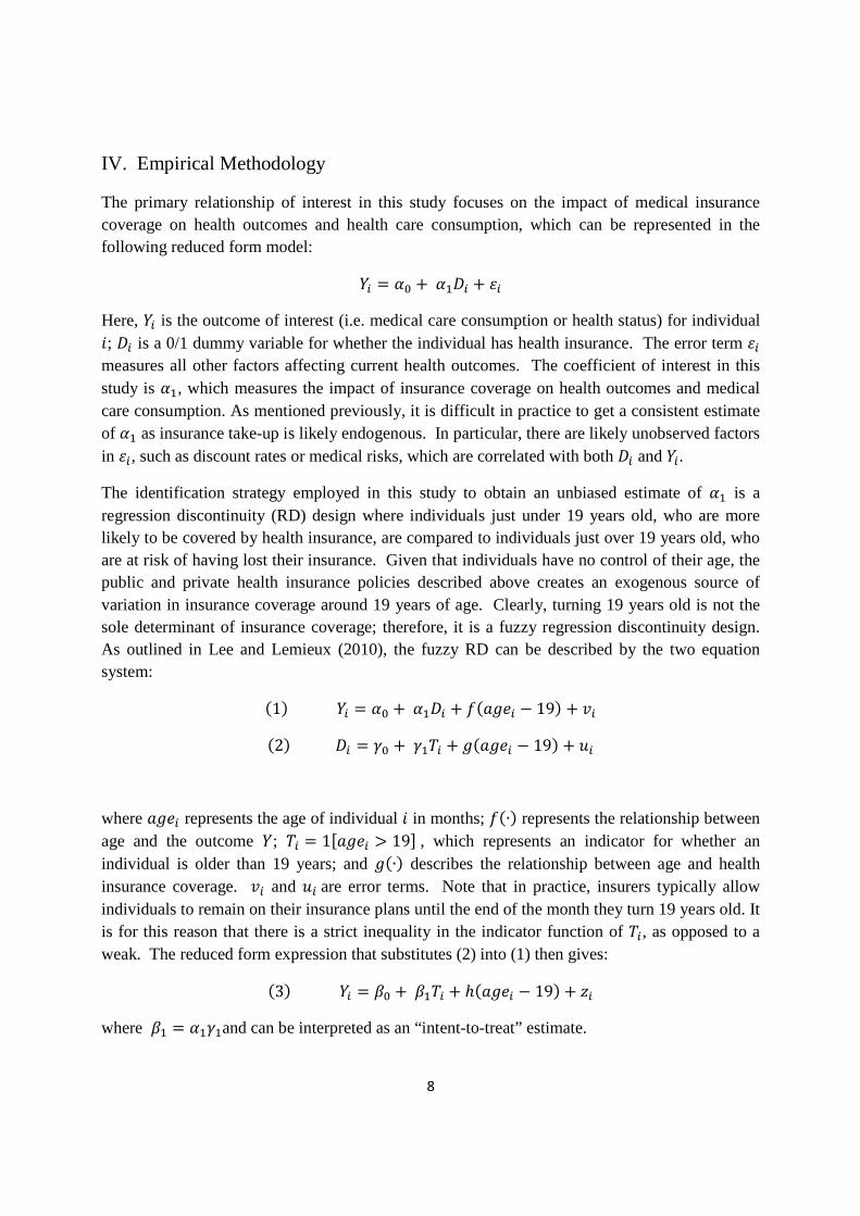
The primary relationship of interest in this study focuses on the impact of medical insurance coverage on health outcomes and health care consumption, which can be represented in the following reduced form model:

�� = �� +�� + �

Here, �� is the outcome of interest (i.e. medical care consumption or health status) for individual �; � is a 0/1 dummy variable for whether the individual has health insurance. The error term � measures all other factors affecting current health outcomes. The coefficient of interest in this study is ��, which measures the impact of insurance coverage on health outcomes and medical care consumption. As mentioned previously, it is difficult in practice to get a consistent estimate of �� as insurance take-up is likely endogenous. In particular, there are likely unobserved factors in �, such as discount rates or medical risks, which are correlated with both � and ��.

The identification strategy employed in this study to obtain an unbiased estimate of �� is a regression discontinuity (RD) design where individuals just under 19 years old, who are more likely to be covered by health insurance, are compared to individuals just over 19 years old, who are at risk of having lost their insurance. Given that individuals have no control of their age, the public and private health insurance policies described above creates an exogenous source of variation in insurance coverage around 19 years of age. Clearly, turning 19 years old is not the sole determinant of insurance coverage; therefore, it is a fuzzy regression discontinuity design. As outlined in Lee and Lemieux (2010), the fuzzy RD can be described by the two equation system:

�1�� = �� +�� + �� − 19� + ��

�2�� = �� +�� + �� − 19� + ��

where �� represents the age of individual � in months; ��∙� represents the relationship between age and the outcome �; �� = 1�� > 19�, which represents an indicator for whether an individual is older than 19 years; and ��∙� describes the relationship between age and health insurance coverage. �� and ��are error terms. Note that in practice, insurers typically allow individuals to remain on their insurance plans until the end of the month they turn 19 years old. It is for this reason that there is a strict inequality in the indicator function of ��, as opposed to a weak. The reduced form expression that substitutes (2) into (1) then gives:

�3�� = �� +�� + ℎ�� − 19� + !�

where �� = ��and can be interpreted as an “intent-to-treat” estimate.

9

Estimation of the fuzzy RD can be performed using either local linear regressions or global polynomial regressions, with this study presently employing the latter approach (i.e. polynomial regressions). One advantage of the polynomial regressions is that it is a simple way of relaxing linearity assumptions and provides some flexibility in the regression function. A disadvantage of this approach, however, is that it relies on data further away from the cutoff of 19 years to estimate the jump at the cutoff. An additional disadvantage is that polynomial regressions are more sensitive to outliers.

Lee and Lemieux (2010) note that if the same order of polynomial is used for ��∙� and ��∙�, then two-stage least-squares (2SLS) estimates of �� are numerically identical to the ratio of the coefficients ��/��. Thus, in this study, the reduced form equations (2) and (3) will be individually estimated to obtain ��. The key in obtaining unbiased estimates using this approach is choosing the order of the polynomial. Consequently, estimation will be done with different specifications in age, including linear, quadratic, cubic, and quartic polynomials to examine the sensitivity of the results under each specification. In future work, I will use a general cross-validation procedure to choose the appropriate order of polynomial. Additionally, splines are used to allow for different age slopes on either side of the cutoff of 19 years. It should be noted that in the RD design, covariates need not be included in estimation; however, they may help with variance reduction. In this paper, I present estimates both with and without covariates and examine the extent to which the estimates vary. The controls included are: dummies for gender, white race, live in a MSA, full-time student, married, still live with parents, survey year, as well as a categorical variables indicating family income as a percentage of the poverty line.

The interpretation of the fuzzy RD estimate requires some attention. First, just as in the case of 2SLS, the estimate of �� can be interpreted as a Local Average Treatment Effect (LATE) under certain conditions, which will be described below. The LATE measures the average treatment effect for those individuals who had insurance prior to turning 19 years old but who age out of their insurance plans on their 19th birthday (i.e. the “compliers” in language of Angrist and Imbens 1994). This means that the fuzzy RD estimate only measures the average effect of insurance coverage on health outcomes and medical care use for a subgroup of the entire population. Secondly, as in any RD design, the estimated impact of health insurance on outcomes can only be identified at the cutoff, which is 19 year olds in this case. That is, while the results may shed light on the effect of health insurance for other age groups, particularly young adults, the estimates derived in this paper are only unbiased for 19 year olds.

The conditions under which the fuzzy RD gives unbiased estimate of the LATE are monotonicity and excludability. In this study, monotonicity rules out that some uninsured individuals take up insurance on their 19th birthdays. Excludability implies that turning 19 years old cannot impact any of the outcomes of interest except through affecting the probability of losing insurance coverage. This amounts to assuming that #��|�� = �� is continuous � = 19 and rules out other factors correlated with health outcomes to change discontinuously on the 19th birthday.

10

This assumption could be violated if say, employment patterns, school attendance, or health lifestyle behaviour changed discontinuously at 19 years old. However, given that age is measured in months, as opposed to years, it is unlikely that these factors would change discontinuously within one or two months of turning 19 years old. As noted by ADG (2011), the most obvious cofounder might be high school graduation and the ensuing transition to college or employment. However, given that graduation typically occurs at the end of June in a year and that birthdays are distributed throughout the year, these factors should not bias the estimates. As a robustness check, I examine whether certain covariates change discontinuously at 19 years. Clearly, this exercise cannot be done with unobservable cofounders; however I confirm observable characteristics do not change discontinuously at 19 years which provides support that the identification strategy employed is valid.

V. Data

The data used in this study comes from the Medical Expenditure Panel Survey (MEPS), a comprehensive dataset on health care utilization, insurance coverage, and medical expenditures. It is produced by the Agency for Healthcare Research and Quality. MEPS draws from a nationally representative sample of US families and individuals, with a rolling panel design. Each individual is interviewed five times over two full calendar years. Every year, a new panel of approximately 15,000 individuals is added to the survey. Thus, two panels are always overlapping at any given point in time, resulting in roughly 30,000 individuals being interviewed each year. Initiated in 1996, the MEPS has interviewed 15 panels of individuals to date.

In each round of interviews, individuals are asked about their general health status, any health conditions they are experiencing, as well as information on their insurance coverage. If they report being insured, detailed information is collected on the type of insurance (eg. Medicaid/SCHIP, employer, etc.) and the holder of the insurance policy (e.g. father, spouse). Individuals are also asked about the medical services they used over the period, such as physician visits, outpatient services, or prescription refills, and the frequency with which they used them. Additionally, information on the costs of services and source of payment for care is collected. To supplement and verify the accuracy of information received from individuals, MEPS also obtains information from those medical providers which individuals reported to have visited. These medical providers include hospitals, physicians, and pharmacies. Information collected includes date of the visit, diagnosis, medical procedures taken, and prescriptions written or filled. In addition to the detailed information on health status and medical care utilization, MEPS also collects basic demographic characteristics, employment and education status, and income. In the public use data, which I use in this study, there is no information on which state individuals reside.

11

In terms of insurance coverage, MEPS collects information on whether the individual is covered for each month in the survey, resulting in up to 24 observations for each individual’s coverage. Additionally, the type of insurance coverage is noted (employer-sponsored, Medicaid/SCHIP) each month. In this project, I examine the impact of turning 19 on three insurance outcomes: whether the individual has any type of medical insurance plan (private or public); whether the individual has private insurance; and whether the individual is covered under public insurance.

The main outcome variables of interest in my study include indicators of general health and non-urgent health care use. To measure health, I examine self-reported health. This is a 5 point scale (excellent, good, fair, poor, weak) and individuals are asked at each interview. I create two dummies for whether the individual reported being in excellent health (1 if excellent health; 0 otherwise) or at least good health (1 if excellent or good health; 0 otherwise). The other measure of health is whether the individual missed school or work in the last two weeks due to being ill. I create two dummies indicating whether the individual missed any school (1 if miss school; 0 otherwise) or missed any work (1 if miss work; 0 otherwise). In constructing these dummies, I only include individuals who reported being in school or work.

To measure non-urgent medical care consumption, I focus on physician visits, dentist, visits, and prescription refills. Additionally, I look at visits relating to mental health issues. I construct dummies for whether the individual had a particular type of visit for each month they are in the sample. In this analysis, I exclude any visits relating to pregnancies as expecting women are covered under Medicaid and are consequently very likely to be insured.

The sample that I use in my analysis includes all individuals who are age 16 to 22 years old, corresponding to a window width of 36 months on each side of the cutoff. I only look at years 1997 to 2006 due to state and federal policies. In particular, SCHIP is the main public insurer for older children and it was only implemented in 1997. Additionally, given I do not have information on the state of residence, I cannot exclude from the analysis those states which mandated extended private coverage beyond 19 years old in recent years. Given most of the state policies were implemented after 2006, I do not include years after 2006. Thus, my sample includes individuals aged 16 to 22 for years 1997-2006.

Descriptive statistics are presented in Table 1. This table shows the means and standard errors of insurance coverage, health indicators, and medical care consumption for those 19 years and under and those older than 19. This table shows that roughly 77% of individuals under 19 have health insurance. This number drops to 58% for the 19 to 22 year olds, which is almost a 20% drop in the proportion insured. This pattern is consistent with individuals aging out of their insurance plans. Almost 8% of this drop comes from changes in private insurance, where 53% of those 19 years and under are insured yet only 45% of those over 19 have private insurance. Similarly, the drop in public insurance is about 11%, where just over 26% of those less than 19 year are covered under public insurance compared to 15% of those over 19 years.

12

In terms of health indicators, 43% of younger individuals consider themselves to be in excellent health and 73% in good or excellent health. Meanwhile, the older cohort considers themselves to be less healthy, with only 36% of individuals considering themselves in excellent health and 70% in good or excellent health. There is a slight difference in the proportion of individuals missing work due to illness between the two groups, with 18% of those 19 years and under and 20% of those over 19 years missing school. The difference in the proportion who miss work due to illness is larger, with a greater proportion of the younger cohort missing work (23%) compared to those over 19 years (13%). In regards to medical care consumption, roughly 12% of individuals under 19 years old have had a doctor visit in any given month, while only 9% of the older age group visit the doctor. The gap is larger for dental visits, with almost 7% of the younger group having a visit compared to less than 4% of those over 19. There is very little difference in terms of the proportion who fill prescriptions in any given month, making up about 27% of each group.

VI. Preliminary Results

Change in Insurance Coverage Rates at age 19

The impact of turning 19 on insurance coverage is shown in Table 2. The regression discontinuity coefficients at age 19 are reported for various age polynomials. The dependent variables examined in this table are dummy variables for: any insurance coverage, private insurance, and public insurance. Estimates are shown with and without controls. As can be seen for all dependent variables, the probability of having insurance significantly drops once individuals hit their 19th birthday. The estimates are generally quite similar in size when controls are included. Additionally, the lower order polynomials give much larger estimates than the higher order polynomials. For example, there is a 10.7% drop in the probability of having any insurance under the linear specification without controls, whereas the drop is 3.3% under the quartic. Note that the mean of insurance coverage for the sample is 68.6%, so consequently the size of these drops is not trivial. In terms of private insurance, the linear specification shows a 6% drop, whereas the quartic gives a 3.2% decline. The proportion of individuals in the sample with private insurance is 49.1%. The fall in public insurance coverage is much smaller, with the linear specification estimating a 4.8% drop, the cubic a 1.4% fall, and the quartic no change in the probability of public insurance coverage. At the same time, only 21.3% of individuals have public insurance, so the size of the estimated declines are still non trivial in the case where they are nonzero.

Figures 1 to 3 provide a sense of how well the models fit the data. The circles show the unconditional averages of insurance coverage for each age in months, while the solid line gives the predicted values in equation (3). Each panel represents a different age polynomial specification. As can be seen in Figure 1, the linear specification overestimates the RD estimates

13

(panel a), as do the quadratic and the cubic to a lesser extent, whereas the quartic seems to fit the raw data quite well (panel d). Note that even prior to turning 19 years old, there is a slow decline in coverage rates with age. This is likely caused by individuals gradually moving out of their parents’ house, resulting in their no longer being considered dependents under health insurance regulations, as discussed above. Figure 2 illustrates the case of private insurance. Again, the quartic in age seems to fit the data best, with the lower order polynomials overestimating the size of the decline at 19 years. The case of changes in public insurance coverage is shown in Figure 3. Here, it appears that the cubic and quartic fit the data best, with the cubic appearing to slightly overestimate the change at 19 years and the quartic perhaps slightly underestimating it.

Table 3 provides the RD estimates for different demographic groups. There is a 2.9% fall in the proportion of males covered upon turning 19 years, compared to 3.4% of females, with a relatively larger drop in public insurance for males (2.7%) and a larger change in private insurance for females (4.3%). Additionally, the decline in insurance coverage is 4% for Whites, whereas Blacks show no significant drop. As expected, those who are not full time students experience a larger decline in insurance coverage (4.3%) compared to students (2.1%). Additionally, the size of insurance loss is larger for those who remain at home (i.e. “dependents”) at 4.2% compared to those who have moved out of the home (1.6%), with the largest decline coming from private insurance (3.9%) for those who don’t leave home.

The results in this section show that the 19th birthday plays a significant role in insurance coverage rates in the US. The estimated drop in insurance coverage rates is at least 3.3% for all insurance types, 3.2% for private insurance, and 0 to 1.4% for public insurance. ADG use local linear regression and must adjust for the bias in their dataset that arises from only seeing individuals who present themselves in the emergency department. They find slightly larger estimates than those derived here, with just over 6% of individuals losing any insurance coverage and 8% of individuals losing private insurance upon turning 19. The next section provides the reduced form effects of turning 19 on health outcomes and medical care consumption.

Change in Health Outcomes at age 19

Table 4 examines equation (3) where self-reported health is the outcome of interest. This table shows that turning 19 years old has little effect on being in excellent health or on being in at least good health (i.e. good or excellent health). In the case of being in at least good health, the estimates are very close to zero; however, in the case of excellent health, the estimates are of a slightly larger scale, yet the size of the standard errors do not allow significant effects to be determined. Figure 4 shows the raw data as well as the predicted values from the regression analysis with the quadratic and quartic specifications. The raw data is noisier than in the case of insurance coverage; however, it appears that there is no noticeable drop in health status at 19 years old that is distinguishable from changes at other ages for both the case of excellent health and at least good health.

14

The estimates in Table 5 show that no effects can be detected in the probability of missing any work or school once individuals hit 19 years. In the case of missing any work, the estimates under the quadratic and cubic specifications show an increase in the probability of missing any work; however, the standard errors cannot reject zero effect. In the case of the probability of missing school, the linear specification shows a decline in the proportion who miss school at age 19, whereas the other specifications show zero effect and are relatively small in size. Figure 5 shows the raw data and the results under different polynomial specifications.

This study does not find evidence that insurance loss leads to a deterioration of health. One caveat is that this study can only examine the immediate impacts of losing insurance coverage on health status, given the nature of the RD design employed. Thus, there may be long term impacts of not having insurance on an individual’s health status, particularly since health is a stock and not a flow; however, this study can only identify immediate effects of insurance loss and finds there is no immediate impact on health status.

Change in Medical Care Consumption at age 19

Table 6 shows the RD estimates for medical care consumption. With the exception of the linear specification, no effect of turning 19 on office visits can be detected. These estimates are quite precise, being close to zero with small standard errors. The inclusion of controls largely does not change the estimates. These findings may be explained by the fact that doctor visits are relatively inexpensive compared to other forms of medical care consumption, such as hospital and emergency department visits. Thus, it appears individuals do not forgo routine care when they lose insurance. Visits relating to mental illness also show no change overall and the estimates are tight. In terms of dental visits, there is a decline in visits of 0.007 to 0.008 percent, which is about 15% of the average proportion of visits (0.054). The estimates for the probability of filling a prescription upon turning 19 are quite noisy, with some specifications giving positive estimate and others giving negative, with the standard errors being relatively large. Figures 6 and 7 plot the raw medical care consumption data along with the predicted values from regression analysis.

VII. Robustness Checks (some to do later)

This section outlines robustness checks which have already been implemented and discusses future work that will be done.

To investigate whether other factors affecting health also change discretely at age 19, I have examined the incidence of being a student, working, and leaving home. I estimate equation (3) with these variables as dependent variables. No discrete change at age 19 was found for any of these variables. Figure 8 shows plots the unconditional averages of these variables along with predicted values from the quartic specification. As can be seen, there is no change in the

15

probability of being a student, working, and leaving home once the 19th birthday is reached. This provides support for the validity of the research design, as was discussed in the section on empirical methodology.

Further checks will be performed in the future to assess the robustness of the results. First, a more formal approach will be taken in choosing the order of the polynomial, specifically a generalized cross-validation procedure such as the Akaike information criterion (AIC) of model selection. Additionally, local linear regressions will be employed with optimal bandwidth choice to investigate the robustness of the results. One advantage of the local linear regression estimator is that it is less sensitive to observations away from the cutoff of 19 years, which is more aligned with the thought process of the RD design which amounts to comparing observations close to, but on opposing sides of the cutoff. In addition, as noted by McCrary and Royer (2011), the local linear estimator is more flexible in accommodating regression functions of various shapes.

Additionally, the standard errors have yet to be adjusted in such a way that accounts for serial correlation among an individual who appears multiple times in the dataset. At the moment, standard errors are merely clustered by age and no correction has been done to reflect the panel nature of the dataset.

Other robustness checks that can be employed include exploiting the panel nature of the data. In particular, first-difference estimates can be performed, where the variation being exploited is now at the individual level and compares outcomes for a given person before and after they turn 19 years. This would be a more robust estimate; however, fewer observations can be included which consequently can lead to noisier estimates. Additionally, it is also possible to look at heterogeneous treatment effects at the individual nature, given the panel dimension of the data, to develop a better understanding of which individuals in particular are most affected by insurance coverage.

Further work will also look at whether there are any anticipation effects, such as individuals “stocking up” on medical care services prior to turning 19 and losing care. If there are anticipation effects, then this would lead to the estimates in this paper being upward biased. However, recent work by Gross (2010) who uses another dataset finds little evidence this is the case as young adults are likely uncertain as to exactly when they lose their coverage. Nevertheless, it would be important to investigate the extent to which this occurs in the MEPS for the outcomes of interest.

VIII. Conclusion

This paper finds that the 19th birthday plays a significant role in insurance coverage rates in the US. The estimated reductions in insurance coverage is at least 3.3% for all insurance types,

16

3.2% for private insurance, and 0 to 1.4% for public insurance. These estimates are slightly smaller in scale than those derived in the ADG paper.

This study finds no immediate effect of insurance loss on health status. As it was noted, there may be long term impacts of not having insurance, particularly since health is a stock and not a flow; however, given the nature of the RD design explored in this paper, only immediate effects can be examined.

Similarly, this study finds no effect of insurance loss on physician office visits or visits related to mental illness. This may be explained by the fact that doctor visits are relatively inexpensive compared to other forms of medical care consumption, such as hospital and emergency department visits. Consequently, it does not appear that young adults forgo routine physician care when they lose insurance. The study does find a decline in dental visits in the order of 15% of average visits, which suggests that dental care is more discretionary than physician visits.

17

References

Anderson, M., Dobkin, C., and Gross, T. (2011). “The Effect of Health Insurance Coverage on the Use of Medical Services.” American Economic Journal: Economic Policy. Forthcoming.

Barber, C., and Nguyen, Q.C. (2009). “Expanding Coverage for Dependents.” Community Catalyst Inc., February 2009 Issue.

Brook, RH., Ware, JE Jr., Rogers, WH., Keeler, EB., Davies, AR., Donald, CA., Goldberg, GA., Lohr, KN., Masthay, PC., Newhouse, JP. (1983). “Does Free Care Improve Adults’ Health? Results from a Randomized Controlled Trial.” New England Journal of Medicine, 309: 1426-1434.

Buchmueller TC., Grumbach K., Kronick R., and Kahn, JG. (2005). “The Effect of Health Insurance on Medical Care Utilization and Implications for Insurance Expansion: A Review of the Literature.” Medical Care Research and Review, 62(1): 3-30.

Busch SH, and Duchovny N. (2005). “Family Coverage Expansions: Impact on Insurance Coverage and Health Care Utilization of Parents.” Journal of Health Economics, 24: 876–890.

Card, D., Dobkin, C., and Maestas, N. (2008). “The Impact of Nearly Universal Insurance Coverage on Health Care Utilization: Evidence from Medicare.” American Economic Review, 98(5): 2242-2258.

Card, D., Dobkin, C., and Maestas, N. (2009). “Does Medicare Save Lives?” Quarterly Journal of Economics, 124(2): 597-636.

Carlson MJ., DeVoe J., and Wright BJ. (2006). “Short-term impacts of coverage loss in a Medicaid population: early results from a prospective cohort study of the Oregon Health Plan.” Annals of Family Medicine, 4: 391-398.

Currie, J. and Gruber, J. (1996). “Health Insurance Eligibility, Utilization of Medical Care, and Child Health.” Quarterly Journal of Economics, 111(2): 431-66.

Dafny, L., and Gruber, J. (2005). “Public Insurance and Child Hospitalizations: Access and Efficiency Effects.” Journal of Public Economics, 89: 109-129.

Department of the Treasury Internal Revenue Service. (2009). “Medical and Dental Expenses (Including the Health Coverage Tax Credit): For Use in Preparing 2010 Returns.” Internal Revenue Service Publication, Cat no. 502. http://www.irs.gov/pub/irs-pdf/p502.pdf.

18

Finkelstein, A., Taubman, S., Wright, B., Bernstein, M., Gruber, J., Newhouse, JP., Allen, H., Baicker, K., and the Oregon Health Study Group (2011). “The Oregon Health Insurance Experiment: Evidence from the First Year.” NBER Working Paper 17190.

Freeman, JD., Kadiyala, S., Bell, J., and Martin, D. (2008). “The Causal Effect of Health Insurance on Utilization and Outcomes in Adults. A Systematic Review of US Studies.” Medical Care, 46(10): 1023-1032.

Hadley J. (2003). “Sicker and Poorer- The Consequences of Being Uninsured: A Review of the Research on the Relationship between Health Insurance, Medical Care Use, Health, Work, and Income.” Medical Care Research and Review, 60(2): 3S–75S.

Hoffman C. and Paradise J. (2008) “Health Insurance and Access to Health Care in the United States.” Annals of the New York Academy of Sciences, 1136: 149-160.

Institute of Medicine. (2001). Coverage Matters: Insurance and Health Care. National Academy Press. Washington, DC.

Keeler, EB. (1992). “Effects of Cost Sharing on Use of Medical Services and Health.” Journal of Medical Practice Management, 8: 317-321.

Levine, PB., McKnight, R., and Heep, S. (2011). “How Effective are Public Policies to Increase Health Insurance Coverage Among Young Adults?” American Economic Journal: Economic Policy, 3: 129-156.

McWilliams, JM., Zaslavasky, AM., Meara, E., and Anyanian, JZ. (2003). “Impact of Medicare Coverage on Basic Clinical Services for Previously Uninsured Adults.” Journal of the American Medical Association, 290(6): 757-764.

National Conference of State Legislatures (2011). Covering Young Adults Through Their Parents’ or Guardians’ Health Policy. http://www.ncsl.org/default.aspx?tabid=14497. (Last accessed September 28th, 2011).

Rosenbach, M., Ellwood, M., Irvin, C., Young, C., Conroy, W., Quinn, B., and Kell, M. (2003). “Implementation of the State Children’s Health Insurance Program: Synthesis of State Evaluations: Background for the Report to Congress.” Mathematica Policy Research Inc, MPR Reference 8644-100.

Shwartz, K., and Damico, A. (2010). “Aging Out of Medicaid: What Is the Risk of Becoming Uninsured?” Kaiser Commission on Medicaid and the Uninsured, March 2010. http://www.kff.org/medicaid/upload/8057.pdf.

FIGURES

.5.6

.7.8

.9P

ropo

rtio

n C

over

ed

16 17 18 19 20 21 22age

(a) Linear in Age (Spline)

.55

.6.6

5.7

.75

.8P

ropo

rtio

n C

over

ed

16 17 18 19 20 21 22age

(b) Quadratic in Age (Spline)

.55

.6.6

5.7

.75

.8P

ropo

rtio

n C

over

ed

16 17 18 19 20 21 22age

(c) Cubic in Age (Spline)

.55

.6.6

5.7

.75

.8P

ropo

rtio

n C

over

ed

16 17 18 19 20 21 22age

(d) Quartic in Age (Spline)

Figure 1: Insurance Coverage by Specification

.44

.46

.48

.5.5

2.5

4P

ropo

rtio

n C

over

ed

16 17 18 19 20 21 22age


.44

.46

.48

.5.5

2.5

4P

ropo

rtio

n C

over

ed

16 17 18 19 20 21 22age


.44

.46

.48

.5.5

2.5

4P

ropo

rtio

n C

over

ed

16 17 18 19 20 21 22age


.44

.46

.48

.5.5

2.5

4P

ropo

rtio

n C

over

ed

16 17 18 19 20 21 22age


Figure 2: Private Insurance Coverage by Specification

.15

.2.2

5.3

Pro

port

ion

Cov

ered

16 17 18 19 20 21 22age


.15

.2.2

5.3

Pro

port

ion

Cov

ered

16 17 18 19 20 21 22age


.1.1

5.2

.25

.3P

ropo

rtio

n C

over

ed

16 17 18 19 20 21 22age


.15

.2.2

5.3

Pro

port

ion

Cov

ered

16 17 18 19 20 21 22age


Figure 3: Public Insurance Coverage by Specification

.3.3

5.4

.45

.5

Pro

port

ion

16 17 18 19 20 21 22age

(a) Excellent Health: Quadratic in Age

.3.3

5.4

.45

.5P

ropo

rtio

n

16 17 18 19 20 21 22age

(b) Excellent Health: Quartic in Age

.66

.68

.7.7

2.7

4.7

6

Pro

port

ion

16 17 18 19 20 21 22age

(c) Good Health: Quadratic in Age

.66

.68

.7.7

2.7

4.7

6P

ropo

rtio

n

16 17 18 19 20 21 22age

(d) Good Health: Quartic in Age

Figure 4: Change in Self-Rated Health

.1.1

5.2

.25

Pro

port

ion

16 17 18 19 20 21 22age

(a) Miss Work: Quadratic in Age

.1.1

5.2

.25

Pro

port

ion

16 17 18 19 20 21 22age

(b) Miss Work: Quartic in Age

.1.1

5.2

.25

.3P

ropo

rtio

n

16 17 18 19 20 21 22age

(c) Miss School: Quadratic in Age

.1.1

5.2

.25

.3P

ropo

rtio

n

16 17 18 19 20 21 22age

(d) Miss School: Quartic in Age

Figure 5: Change in Miss Any Work/School

.08

.1.1

2.1

4

offic

e_v

isit

16 18 20 22age

(a) Office Visit: Quadratic in Age

.08

.1.1

2.1

4

Pro

por

tion

16 18 20 22age

(b) Office Visit: Quartic in Age

.02

.04

.06

.08

.1

Pro

por

tion

16 18 20 22age

(c) Dentist Visit: Quadratic in Age

.02

.04

.06

.08

.1

Pro

por

tion

16 18 20 22age

(d) Dentist Visit: Quartic in Age

Figure 6: Change in Doctor and Dentist Visits at Age 19

.24

.26

.28

.3.3

2P

ropo

rtio

n

16 18 20 22age

(a) Fill Prescription- Quadratic in Age

.24

.26

.28

.3.3

2

Pro

port

ion

16 18 20 22age

(b) Fill Prescription- Quartic in Age

.005

.01

.015

.02

Pro

port

ion

16 18 20 22age

(c) Mental Illness Visit: Quadratic in Age

.005

.01

.015

.02

Pro

port

ion

16 18 20 22age

(d) Mental Illness Visit: Quartic in Age

Figure 7: Change in Prescription Refills and Mentall Illness Visits

.2.4

.6.8

Pro

port

ion

17 18 19 20 21 22age

(a) Student

0.2

.4.6

.8P

ropo

rtio

n

16 17 18 19 20 21 22age

(b) Work

.4.5

.6.7

.8.9

Pro

port

ion

16 17 18 19 20 21 22age

(c) Don't Leave Home

Figure 8: Robustness Checks on Covariates- Quartic Specification

Variable 19 Years and Under Over 19 Years

Insurance Coverage

Any Insurance 0.772 0.582[0.419] [0.493]

Private Insurance 0.529 0.446[0.499] [0.497]

Public Insurance 0.264 0.153[0.441] [0.36]

Health Status Indicators

Excellent Health 0.431 0.361[0.495] [0.48]

Good Health 0.732 0.696[0.443] [0.46]

Miss Work 0.181 0.204[0.385] [0.403]

Miss School 0.231 0.129[0.422] [0.335]

Medical Care Consumption

Any Office Visit 0.116 0.090[0.32] [0.286]

Any Dentist Visit 0.069 0.037[0.254] [0.188]

Any Prescription 0.275 0.271[0.447] [0.445]

Any Visit for Mental Illness 0.014 0.009[0.117] [0.094]

Number of Individuals in Sample

Number of Observations (Maximum) 455,407

25,572

Table 1: Means by Age Group

Note: All variables were coded as 0/1 dummy variables, so the statistics reflect the proportion of individuals meeting the specific criteria. Standard errors in brackets. Those 19 years and under comprise of 16 to 19 year olds, while those over 19 years are those between 19 and 22 years of age. Given that individuals were sampled multiple times over the sample period, the number of observations is greater than the number of individuals. Since insurance coverage is asked every month and medical care consumption is measured each month, individuals form up to 24 observations in the dataset.

TABLES

Specification for Age

Mean of Dependent Variable

RD Estimates

Linear -0.107 -0.091 -0.06 -0.048 -0.048 -0.048[0.008]*** [0.007]*** [0.004]*** [0.003]*** [0.004]*** [0.005]***

Quadratic -0.066 -0.059 -0.042 -0.033 -0.029 -0.031[0.007]*** [0.007]*** [0.004]*** [0.004]*** [0.004]*** [0.005]***

Cubic -0.054 -0.053 -0.041 -0.038 -0.014 -0.018[0.009]*** [0.010]*** [0.007]*** [0.007]*** [0.003]*** [0.004]***

Quartic -0.033 -0.032 -0.032 -0.028 0 -0.004[0.006]*** [0.007]*** [0.007]*** [0.006]*** [0.003] [0.004]

Covariates No Yes No Yes No Yes

Number of Observations 343,847 215,029 343,847 215,029 343,847 215,029

Notes: The RD coefficients at age 19 are reported. Data come from the Medical Expenditure Panel, years 1997-2006. These results were derived from OLS regression on age month cell means, where the weights are given by the number of observations in each age month grouping. Splines were estimated on either side of the 19 years cutoff. Covariates include dummies for male, white, msa, full-time student, married, never leave home, survey year, as well as indicators for family income as a percentage of poverty line. Robust standard errors in brackets. Standard errors were clustered by age (in months). * significant at 10%; ** significant at 5%; *** significant at 1%

Table 2: Change in Insurance Coverage Rates at 19

Any Insurance Private Insurance Public Insurance

0.686 0.491 0.213

Any Insurance Private Insurance Public Insurance No. Observations

Sample Group

Males -0.029 -0.020 -0.027 169,906[0.005]*** [0.003]*** [0.005]***

Females -0.034 -0.043 -0.002 173,941[0.007]*** [0.010]*** [0.003]

Whites -0.04 -0.039 -0.011 259,898[0.007]*** [0.008]*** [0.002]***

Blacks -0.003 -0.012 -0.014 61,018[0.005] [0.007]* [0.005]***

Students -0.021 -0.016 -0.019 131,752[0.005]*** [0.006]*** [0.004]***

Non-Students -0.043 -0.042 -0.010 138,387[0.008]*** [0.009]*** [0.002]***

Leave Home -0.016 -0.016 -0.016 125,677[0.007]** [0.005]*** [0.005]***

Don't Leave Home -0.042 -0.039 -0.017 218,170[0.005]*** [0.007]*** [0.003]***

Covariates No No No -

Age Specification Quartic Quartic Cubic -

RD Estimates

Notes: The RD coefficients at age 19 are reported. Data come from the Medical Expenditure Panel, years 1997-2006. These results were derived from OLS regression on age month cell means, where the weights are given by the number of observations in each age month grouping. Splines were estimated on either side of the 19 years cutoff. No covariates are included. Robust standard errors in brackets. Standard errors were clustered by age (in months). * significant at 10%; ** significant at 5%; *** significant at 1%

Table 3: Change in Insurance Coverage Rates at 19 by Demographic Group

Overall Mean of Dependent Variable

0.686 0.491 0.213 343,847



RD Estimates

Linear -0.021 -0.017 -0.006 0

[0.008]** [0.010] [0.007] [0.009]

Quadratic -0.010 -0.015 0.001 0[0.011] [0.014] [0.011] [0.012]

Cubic -0.017 -0.022 -0.003 -0.002[0.014] [0.018] [0.015] [0.017]

Quartic -0.019 -0.032 -0.014 -0.024[0.020] [0.022] [0.022] [0.023]

Covariates No Yes No Yes

Number of Observations 72,589 47,268 72,589 47,268


Table 4: Change in Self Reported Health Status at 19

Excellent Health Good Health

0.399 0.716



RD Estimates

Linear 0.007 0.005 -0.060 -0.038

[0.011] [0.015] [0.012]*** [0.012]***

Quadratic 0.024 0.003 -0.008 0.003[0.016] [0.021] [0.012] [0.013]

Cubic 0.022 0.01 0.008 0.017[0.022] [0.024] [0.015] [0.015]

Quartic 0.001 0.026 0.019 0.020[0.027] [0.022] [0.019] [0.018]

Covariates No Yes No Yes

Number of Observations 72,589 22,636 72,589 22,636

0.202 0.196


Table 5: Change in Days Missed School or Work at 19

Miss Any Work Miss Any School



RD Estimates

Linear -0.014 -0.014 0.001 0.002 -0.004 -0.005 -0.017 -0.017

[0.002]*** [0.002]*** [0.001]** [0.001]** [0.002]*** [0.002]** [0.007]*** [0.007]**

Quadratic -0.005 -0.005 0.001 0.002 -0.007 -0.008 -0.009 -0.022[0.005] [0.004] [0.001] [0.002] [0.002]*** [0.003]** [0.011] [0.011]**

Cubic -0.008 -0.009 0 -0.001 -0.008 -0.013 -0.014 -0.022

[0.005] [0.004]** [0.001] [0.001] [0.004]** [0.005]*** [0.015] [0.013]*

Quartic -0.005 -0.005 0 0.002 -0.008 -0.008 0.007 0.018[0.005] [0.004] [0.001] [0.002] [0.004]** [0.005]* [0.015] [0.008]**

Covariates No Yes No Yes No Yes No Yes

Number of Observations 343,847 215,109 343,847 215,109 343,847 215,109 72,589 47,306

Table 6: Change in Medical Care Consumption at 19

Office Visits Visit for Mental Illness Dentist Visit Filled Prescription

0.104 0.012 0.054 0.273


1

The Impact of Spousal Health Shocks on Perceptions of Health and Preventative Health Behaviour

By: Lori Timmins

I. Introduction

This research paper explores whether new information, acquired through exogenous health shocks of family members, causes individuals to change their perceptions of own health and their health-related behaviour. In particular, the types of health shocks that will be examined include: acute health conditions, such as heart attacks and strokes, the diagnosis of chronic illnesses, such as hypertension and diabetes, and accidental injuries and falls. The manner in which individuals and their spouses respond to the health shock is the subject of this study, with a focus on spousal health behaviour. The outcomes of interest centre on broad preventative health measures, such as medical screenings, physical exercise, and alcohol and cigarette consumption. Additionally, perceptions of health, as measured by self-reported health and expected longevity, will be examined.

This research question could provide insight into the manner in which individuals respond to new health information. In particular, an increase in certain types of preventative health care could indicate the importance of saliency of illness and poor health habits in shaping health behaviour. For example, if cancer screening is more responsive to a cancer diagnosis than say to a visit to the emergency department for injury, then this suggests saliency plays a role. Along these lines, Becker and Mulligan (1997) develop a theoretical model where an individual’s discount factor is affected by the ability to visualize the future, which in turn affects the optimal stream of consumption (health consumption in the present case). In this context, being able to better visualize the consequences of poor health may result in individuals changing their health behaviour. The goal of this research project is to explain any findings in the context of a theoretical model. Additionally, by examining how outcomes are affected by different health shocks, I will try to disentangle the mechanisms that give rise to the results.

II. Previous Literature

To date, only a handful of studies have examined the impact of family health shocks on health perception and behaviour. The bulk of this literature focuses on smokers and cigarette consumption and centres on the impact of own health shocks. Smith et al. (2001) examine how health shocks affect the expected longevity of smokers. They find that smokers react quite differently than non-smokers after experiencing health shocks in how they form beliefs about

2

their longevity. In particular, smokers update their beliefs more dramatically when the shock is smoking related. The authors also examine spousal health shocks on perceived longevity, finding no effect for both smokers and non-smokers. One drawback of the Smith et al. (2001) study is that it focuses entirely on risk-updating and largely ignores changes in health behaviour associated with the health shock that may in turn affect perceived health and longevity.

Clark and Etile (2002) examine the impact of changes in self-reported health status, check-ups, and chest or heart problems on the cigarette consumption of British adults. Instrumenting for current consumption with lagged consumption, the authors find that individuals reduce cigarette use when their health declines; however, they do not alter their consumption when their spouses’ health deteriorates. This study is narrow in scope in that it centres on an addiction model for cigarette consumption. Thus, it cannot speak directly to the impact of health shocks on other dimensions of health related behaviour, particularly preventative health, such as obtaining medical screenings, doing physical exercise, or managing weight.

Christakis and Allison (2006) find that the hospitalization of one’s spouse increases the risk of death for an individual, and this effect varies with the illness associated with the spouse’s hospitalization. The authors hypothesize that the negative impact of an illness on a partner can work through increased stress; although, they do not do investigate any mediating factors which may play a role. Consequently, it remains uncertain exactly what factors are responsible for the poorer health of individuals whose partners have been hospitalized.

Most of the previous economics literature examining health shocks has focused on how household labour supply is affected. While labour supply is not of prime interest in this study, it may act as a mediating factor in determining health outcomes. The bulk of the studies focusing on health shocks and labour supply find that individuals reduce their labour supply when they themselves experience health problems, as might be expected; however, the impact on a spouse’s labour supply could theoretically go either way. On one hand, individuals may act as caregivers for their unhealthy spouse following a shock, reducing hours worked. Additionally, if there is complementarity of leisure time between couples, this may compel spouses to reduce their labour supply when the unhealthy partner reduces theirs. Conversely, there may be an added worker effect, whereby individuals may increase work hours to compensate for any forgone wages of the unhealthy spouse. The handful of empirical studies examining this generally do not find strong evidence of the added work effect. For example, Coile (2004) finds that men slightly increase their work hours following a health shock to their wives; although it’s very small in size in comparison to the reduction in their own labour supply. There is no added worker effect for women, on average; however, they modestly reduce their work hours when their husband’s shock is severe. Gallipoli and Turner (2009) also find scant evidence of an added worker effect, particularly for wives. These results are aligned with women acting as caregivers for their unhealthy spouse. Charles (1999), on the other hand, examines spouse disability status and self-reported health and find that men reduce their labour supply quite substantially in response to wives’ poor health, whereas women significantly increase theirs when their husbands are ill.

3

This study examines how a range of health behaviour is affected by health shocks, with a focus on spousal health shocks. Rather than focusing solely on cigarette consumption or delineating individuals by smoking status, this study examines a broader set of health behaviour such as preventative screenings and routine medical check-ups, physical exercise, and weight management. It also examines how self-reported health and longevity is affected by health shocks, taking into account that changes in health behaviour may affect these perceptions. If any effects are found, possible mechanisms will be examined including saliency and labour supply responses, with the goal of reconciling the findings with a theoretical model.

II. Empirical Methodology

The empirical strategy is to exploit exogenous health shocks between survey interviews to examine their effect on health perception and behaviour. There are two estimating equations of interest which can be used to identify the effect, the first using a difference-in-difference (DD) approach and the second using individual fixed effects (FE). The estimating equation for the DD is as follows:

�1��ℎ�, = �� + ��ℎ��, + ��ℎ�� + �� +

� �� + �!��"ℎ�� + �#��"ℎ�� +

$��% + &��ℎ + '�

Here, ��ℎ�, is individual (’s health outcome of interest in period ; ��ℎ��, is a

dummy for whether individual ( is observed to have had a shock in the past; ��ℎ��, is a dummy for whether individual (’s spouse is observed to have had a

health shock in the past; �� are covariates for individual ( in period ; �� are covariates for individual (’s spouse; ��"ℎ�� is a dummy variable for whether individual ( is ever observed to experience a health shock (i.e. in periods before or after ); and ��"ℎ�� is a dummy variable for whether individual (’s spouse is ever observed to experience a shock. $��% and &��ℎ are year and month fixed effects in period . The coefficients of interest are �� and ��, which estimates the effects of own health shock and spousal health shocks, respectively, on individual (’s health outcomes.

The estimating equation for the FE model is as follows:

�2��ℎ�, = *� + *��ℎ��, + *��ℎ�� + *�� +

* �� + ( +$��% +&��ℎ + +�

All variables are as discussed above, and ( is a fixed effect for individual (. In the FE model, the coefficients of interest are *�and *�.

4

The identifying assumption for both models is that the timing of the health shock is uncorrelated with unobserved changes in health perception or behaviour. That is, ,�'� |��ℎ��, � = 0, ,�'� |��ℎ��, � = 0, ,�+� |��ℎ��, � = 0,

and ,�+� |��ℎ��, � = 0. While to some extent people may anticipate the onset of

illnesses, the actual realization and particularly its timing may be unanticipated. Thus, the unexpected arrival of new health information is used to estimate the effect of changes in own or spousal health on health behaviour and perception. The variation used for estimation of the DD comes from comparing individuals who have and have not experienced health shocks over time. The DD approach allows for unobserved time-invariant factors that is common to all individuals who ever experience their own or their spouse’s health shock. Meanwhile, the variation exploited in the FE approach comes from examining within individuals over time. That is from comparing the same individual before and after the health shock. It is more robust than the DD approach in that it allows for a fixed effect at the individual level rather than a common shock. A sufficiently long panel is required for the FE approach to be able to estimate the individual fixed effects.

The identifying assumption seems quite valid for acute health shocks, such as heart attacks, strokes, and cancer diagnosis. These are also the type of shocks where the largest effects on health behaviour are expected. For the diagnosis of chronic illnesses, such as diabetes or hypertension, the identifying assumption is less innocuous. It may be that the timing of diagnosis is affected by health. This is particularly the case of own health shocks on health behaviour. There are checks I can provide that explores the validity of the identifying assumption. First, I can look at whether observable characteristics, including past health changes, are associated with the timing of diagnosis (e.g. a discrete time hazard model). Additionally, I can also do a sort of “placebo” test by comparing the estimates of simply being evaluated for the illness, but not being diagnosed, on health outcomes. Zero effect would strengthen the identifying assumption.

IV. Data

In this study, there are two datasets which will be used to investigate the impact of spousal health shocks on health perceptions and behaviour. The first is the Medical Expenditure Panel Survey (MEPS), a comprehensive dataset on health care utilization, insurance coverage, and medical expenditures. It is produced by the Agency for Healthcare Research and Quality and draws from a nationally representative sample of US families and individuals. Each individual is interviewed five times over two full calendar years. Every year, a new panel of approximately 15,000 individuals is added to the survey. Thus, two panels are always overlapping at any given point in time, resulting in roughly 30,000 individuals being interviewed each year. Initiated in 1996, the MEPS has interviewed 15 panels of individuals to date.

5

In each round of interviews, individuals are asked about their general health status, any health conditions they are experiencing, as well as information on their medical care consumption. Each year, individuals are asked their BMI and the frequency with which they do physical exercise. MEPS verifies the accuracy of medical care consumption by obtaining information from medical providers individuals reported to have visited, such as hospitals, physicians, and pharmacies. Information collected from these providers includes date of the visit, medical illness, medical procedures taken, and prescriptions written or filled. The medical provider information does not collect information on whether the purpose of the visit was to obtain preventative health screenings; however, individuals are asked annually whether they have received certain screenings over the year, such as routine physicals, blood pressure checks, cholesterol screenings, pap smears, mammograms, and colonoscopies.

In the MEPS, individuals are not asked whether they have experienced specific illnesses. The medical provider information provides a diagnosis for each visit; however, it is difficult to ascertain the actual timing of first diagnosis because medical visits relating to diagnosis, treatment, and management of the illness generally cannot be distinguished from one another. Thus, for the present moment, I focus solely on emergency department visits relating to heart attacks, heart failures, and strokes in order to identify which individuals have experienced a health shock. Given the short time frame in which individuals are sampled in this dataset (i.e. two calendar years), the MEPS can shed light into the immediate effects of health shocks on perceptions of own health and health behaviour.

The other dataset which will be used in this study is the Health and Retirement Survey (HRS), a national longitudinal survey of Americans over 50 years old. The survey collects extensive information on disability, physical health and functioning, income, and employment. Individuals and their spouses are sampled every two years. It was launched in 1992, with the original cohort consisting of individuals born between 1931 and 1941. Every six years, a new birth cohort of individuals over 50 years is added to the sample.

Each wave, the HRS collects information on self-reported health, physical functioning and limitations, as well as prior and current health diagnoses. The survey also collects information on individuals’ expected longevity. In terms of health behaviour, information is collected on preventative screenings such as cholesterol, cancer, blood pressure, and flu shots. In addition, individuals are asked about their physical exercise, cigarette and alcohol consumption, and weight gain/loss. For a subset of individuals, information is also collected on time spent on daily activities, including exercising, cooking at home, eating outside the home, and treating medical conditions.

To identify exposure to health shocks in the HRS, all events that occur between waves and are new, serious health conditions will be treated as a shock. For example, if an individual reported no history of a cancer diagnosis in a previous wave yet reports one in the subsequent wave, then this will be treated as a health shock. Types of health shocks that can be examined in the HRS

6

include types of cancer, heart attacks, strokes, as well as chronic illnesses such as hypertension and diabetes. Given that the HRS interviews biannually, it would be possible to look at longer run effects of spousal health shocks, which the MEPS is not able to do.

The sample that will be used in both the MEPS and the HRS will be all married individuals in the sample. Data from all waves will be used from both datasets.

V. Preliminary Results

Preliminary analysis has been done using the MEPS, focusing on health shocks arising from emergency department visits for heart attacks and strokes. For the moment, these two conditions have been grouped together. Just over 1% of the sample is observed to have experienced a heart attack or stroke (4,242 observations). Out of those that have heart attacks, 64% are male and 36% are female. Note that given the panel nature of the dataset, where individuals are sampled five times, the actual number of individuals with a health shock is less (998 individuals). Only spousal health shocks, the central focus of this paper, have been examined to date using the DD approach. Thus, all estimates reported below are for �� as defined in equation (1) above.

Table 1 shows the impact of spousal heart attacks/strokes on measures of self-reported health. Individuals are asked about their physical and mental health at each interview, where self-reported health is recorded as a 5 point scale (excellent, good, fair, poor, weak). I create a 0 to 1 index for each variable, where a value of 1 indicates excellent health and a value of 0 weak health. Additionally, I create two dummies for whether the individual reported being in excellent health (1 if excellent health; 0 otherwise) or at least good health (1 if excellent or good health; 0 otherwise). This table shows that those whose spouses have suffered a heart attack or stroke report a significant decline in their self-reported physical and mental health after the event. Most of the decline appears to come from individuals no longer reporting to be in good health, rather than changes in being in excellent health. As can be seen, the size of the estimated coefficients is quite large relative to the means. Table 2 examines whether husbands and wives are differentially affected by spousal health shocks. This table shows that husbands are significantly less likely to report being in excellent or good physical health following a health shock compared to females (4.7% difference) and in excellent or good mental health (8% difference). Once a male interaction is added to the specification, the main effects lose their level of significance.

The effects of a spousal health shock on days missed work are shown in Table 3. Here, I create dummies indicating whether the individual missed any work due to own illness or for another individual’s illness (1 if miss work; 0 otherwise). In constructing these dummies, I only include individuals who reported being in work. Additionally, I examine number of days missed work both for those who report missing work as well as for all those who work (i.e. those who do not report missing any work are given a value of 0 for days missed). Interestingly, although

7

individuals report to have a deterioration in health following a health shock of their spouse, there is a decline in the probability of missing work for own illness by 5%. This suggests that perceptions of health, rather than actual health itself, may be driving the results in Table 1. There is a sharp increase in individuals reporting to have missed work for others’ illness following the health shock. On average, those who miss work to care for others miss approximately 3 days of work following the health shock of their spouse. Table 4 examines how these effects vary by gender. As can be seen, the main effects are still significant. Additionally, men are more likely to miss work for own illness and miss more days of work for own illness following their wives’ heart attack. Interestingly, they miss fewer days of work relative to women to care for others.

Tables 5 and 6 examine the impact of spousal health shocks on the frequency of physician office visits in a month. There is no impact on the probability of having an office visit; although there is marginally significant positive effect on the number of office visits. This effect is still detected in the model that adds the interaction with male, and husbands have fewer doctor visits than wives following the health shock of their spouse. Tables 7 and 8 examine the impact of spousal health shocks on preventative health behaviour. There is no effect on preventative health screenings, such as cholesterol and blood pressure checks, and there is no effect on exercising three times a week or more. A positive effect is found for body mass index (BMI); however, the level of significance is marginal (10% significance level). As Table 8 shows, the same patterns persist when a male interaction is added to the specification; however, husbands do not gain as much weight following the health shock of a spouse compared to wives.

Future analysis will include other measures of health shocks and will investigate how outcomes respond to each type of shock. The HRS dataset will be used for analysis, and the fixed effect model will be estimated. Additionally, the findings will be interpreted in the context of theoretical models and possible mechanisms will be examined.

8

References

Becker, G. and Mulligan, CB. (1997). “The Endogenous Determination of Time Preference.” The Quarterly Journal of Economics, 112(3):. 729-758 Charles, K.K. (1999). “Sickness in the Family: Health Shocks and Spousal Labor Supply," Unpublished manuscript, University of Michigan. Christakis, N. A., and Allison, P. D. (2006). “Mortality after the Hospitalization of a Spouse.” New England Journal of Medicine, 354(7): 719-730. Clark, A. and Etile, F. (2002). "Do Health Changes affect Smoking? Evidence from British panel Data," Journal of Health Economics, 21(4): 533-562. Coile, C. (2004). “Health Shocks and Couples' Labor Supply Decisions," NBER Working Paper 10810. Gallipoli, G., and Turner, L. (2009). “Household Responses to Individual Shocks: Disability and Labour Supply.” CLSRN Working Paper, no.23. Smith, V.K., Taylor, D.H., Sloan, F.A., Johsnon, F.R., and Desvousges, W.H. (2001). “Do Smokers Respond to Health Shocks?” The Review of Economics and Statistics, 83(4): 675-687.

Variable Coefficient on Postspouseshock Mean Observations

Self-reported Physical Health (Index) -0.022 0.66 284,253[0.009]**

Excellent Physical Health -0.018 0.24 284,253[0.015]

Excellent or Good Physical Health -0.048 0.57 284,253[0.017]***

Self-reported Mental Health (Index) -0.026 0.75 284,253[0.008]***

Excellent Mental Health -0.01 0.38 284,253[0.017]

Excellent or Good Mental Health -0.056 0.69 284,253[0.016]***

Table 1: The Impact of Spousal Health Shocks on Self-Reported Health

Note: The estimated coefficients measure the impact of a spousal heart attack or stroke on self-reported health outcomes. Robust standard errors in brackets. For the indices, higher values indicate superior health. For excellent and excellent or good health, these two variables were coded as 0/1 dummy variables. Covariates include dummies for male, white, msa, working, age, survey year and month, as well as indicators for family income as a percentage of poverty line. Given that individuals were sampled multiple times over the sample period, the number of observations is greater than the number of individuals. * significant at 10%; ** significant at 5%; *** significant at 1%

Variable Mean Observations

Self-reported Physical Health (Index) -0.016 -0.018 0.66 284,253[0.010] [0.012]

Excellent Physical Health -0.01 -0.022 0.24 284,253[0.017] [0.020]

Excellent or Good Physical Health -0.031 -0.047 0.57 284,253

[0.019]* [0.022]**

Self-reported Mental Health (Index) -0.015 -0.03 0.75 284,253

[0.009]* [0.011]***

Excellent Mental Health -0.003 -0.019 0.38 284,253[0.019] [0.022]

Excellent or Good Mental Health -0.027 -0.081 0.69 284,253[0.018] [0.021]***

Table 2: The Impact of Spousal Health Shocks on Self-Reported Health with Male Interaction

Note: The estimated coefficients measure the impact of a spousal heart attack or stroke on self-reported health outcomes. Robust standard errors in brackets. For the indices, higher values indicate superior health. For excellent and excellent or good health, these two variables were coded as 0/1 dummy variables. Covariates include dummies for male, white, msa, working, age, survey year and month, as well as indicators for family income as a percentage of poverty line. Given that individuals were sampled multiple times over the sample period, the number of observations is greater than the number of individuals. * significant at 10%; ** significant at 5%; *** significant at 1%

Coefficient on Postspouseshock

Coefficient on Postspouseshock x male


Miss Any Work for Own Illness -0.05 0.20 174,272[0.024]**

Days Missed Work for Own Illness (if Miss) 2.417 6.87 34,991[1.814]

Days Missed Work for Own Illness (Everyone) 0.30 1.37 174,272[0.447]

Miss Any Work for Other's Illness 0.135 0.10 190,115

[0.017]***

Days Missed Work for Other Illness (if Miss) 3.085 3.10 19,395[0.893]***

Days Missed Work for Other Illness (Everyone) 1.182 0.31 190,023[0.123]***

Table 3: The Impact of Spousal Health Shocks on Days Missed Work

Note: The estimated coefficients measure the impact of a spousal heart attack or stroke on days missed work. Robust standard errors in brackets. Covariates include dummies for male, white, msa, working, age, survey year and month, as well as indicators for family income as a percentage of poverty line. Given that individuals were sampled multiple times over the sample period, the number of observations is greater than the number of individuals. * significant at 10%; ** significant at 5%; *** significant at 1%


Miss Any Work for Own Illness -0.068 0.052 0.20 174,272[0.026]*** [0.031]*

Days Missed Work for Own Illness (if Miss) -0.943 10.915 6.87 34,991

[1.983] [2.604]***

Days Missed Work for Own Illness (Everyone) -0.606 2.686 1.37 174,272

[0.487] [0.578]***

Miss Any Work for Other's Illness 0.131 0.012 0.10 190,115

[0.018]*** [0.022]

Days Missed Work for Other Illness (if Miss) 3.951 -2.905 3.10 19,395[0.936]*** [0.946]***

Days Missed Work for Other Illness (Everyone) 1.459 -0.813 0.31 190,023[0.135]*** [0.159]***

Table 4: The Impact of Spousal Health Shocks on Days Missed Work with Male Interaction



Note: The estimated coefficients measure the impact of a spousal heart attack or stroke on days missed work. Robust standard errors in brackets. Covariates include dummies for male, white, msa, working, age, survey year and month, as well as indicators for family income as a percentage of poverty line. Given that individuals were sampled multiple times over the sample period, the number of observations is greater than the number of individuals. * significant at 10%; ** significant at 5%; *** significant at 1%


Physician Visit 0.005 20.78 1,358,689[0.006]

Number of Physician Visits (if Go) 0.103 1.88 310,907

[0.053]*

Number of Physician Visits (Everyone) 0.037 0.39 1,358,689[0.019]*

Table 5: The Impact of Spousal Health Shocks on Monthly Physician Office Visits

Note: The estimated coefficients measure the impact of a spousal heart attack or stroke on physician office visits. Robust standard errors in brackets. Covariates include dummies for male, white, msa, working, age, survey year and month, as well as indicators for family income as a percentage of poverty line. Given that individuals were sampled multiple times over the sample period, the number of observations is greater than the number of individuals. * significant at 10%; ** significant at 5%; *** significant at 1%


Physician Visit 0.001 0.009 20.78 1,358,689[0.007] [0.009]

Number of Physician Visits (if Go) 0.149 -0.134 1.88 310,907

[0.059]** [0.079]*

Number of Physician Visits (Everyone) 0.05 -0.035 0.39 1,358,689

[0.021]** [0.027]



Note: The estimated coefficients measure the impact of a spousal heart attack or stroke on phsyician office visits. Robust standard errors in brackets. Covariates include dummies for male, white, msa, working, age, survey year and month, as well as indicators for family income as a percentage of poverty line. Given that individuals were sampled multiple times over the sample period, the number of observations is greater than the number of individuals. * significant at 10%; ** significant at 5%; *** significant at 1%

Table 6: The Impact of Spousal Health Shocks on Monthly Physician Office Visits with Male Interaction


Blood Pressure Screening in Year 0.274 80.42 59,683[0.218]

Cholesterol Screening in Year 0.278 59.01 57,878[0.262]

Flu Shot in Year 0.348 31.72 59,896[0.242]

Pap Smear in Year 0.38 61.54 29,560[0.334]

Breast Exam in Year 0.629 66.07 29,674[0.328]*

Mammogram in Year 0.008 47.48 114,998[0.021]

Colonoscopy in Year -0.73 30.56 12,756[0.460]

Do Physical Exercise 3 x per week 0.022 54.56 264,179[0.018]

BMI 0.388 27.76 238,160[0.221]*

Table 7: The Impact of Spousal Health Shocks on Preventative Health

Note: The estimated coefficients measure the impact of a spousal heart attack or stroke on preventative health care. All variables are expressed as 0/1 dummy variables. Robust standard errors in brackets. Covariates include dummies for male, white, msa, working, age, survey year and month, as well as indicators for family income as a percentage of poverty line. Given that individuals were sampled multiple times over the sample period, the number of observations is greater than the number of individuals. * significant at 10%; ** significant at 5%; *** significant at 1%


Blood Pressure Screening in Year 0.264 0.03 80.42 59,683[0.218] [0.031]

Cholesterol Screening in Year 0.282 -0.011 59.01 57,878[0.263] [0.038]

Flu Shot in Year 0.358 -0.026 31.72 59,896[0.242] [0.035]

Colonoscopy in Year -0.696 -0.103 30.56 12,756[0.460] [0.063]

Do Physical Exercise 3 x per week 0.034 -0.032 54.56 264,179[0.020]* [0.024]

BMI 0.596 -0.56 27.76 238,160[0.247]** [0.301]*

Table 8: The Impact of Spousal Health Shocks on Preventative Health with Male Interaction

Note: The estimated coefficients measure the impact of a spousal heart attack or stroke on preventative health care. All variables are expressed as 0/1 dummy variables. Robust standard errors in brackets. Covariates include dummies for male, white, msa, working, age, survey year and month, as well as indicators for family income as a percentage of poverty line. Given that individuals were sampled multiple times over the sample period, the number of observations is greater than the number of individuals. * significant at 10%; ** significant at 5%; *** significant at 1%

Coefficient on Postspouseshock Coefficient on

Postspouseshock x male

Beyond the Mean: An Examination ofHeterogenous Child Responses to a Universal

Childcare Policy in Quebec

Lori L. Timmins∗

Department of Economics, University of British Columbia

November 1, 2010

Abstract This study examines the impact of a universal childcare policy in Quebec

on the distributions of child motor skills and cognitive development. In 1997, the Quebec

government began offering reduced rate spaces for $5 a day which was accessible to families

from all economic and educational backgrounds. Estimating the impact of the reform on

the marginal distribution of outcomes using a quantile difference-in-differences model, this

paper finds that there is little heterogeneity in the response to the universal childcare policy

across the distributions of motor skills and cognitive outcomes. In fact, this study finds that

the policy had little significant effect on these outcomes at any point along the distributions,

neither for the full sample of children nor when the sample is split by child demographic

characteristics. These results are robust to different specifications and estimation techniques.

∗Address: 997 - 1873 East Mall, Vancouver, BC, V6T 1Z1 Canada, e-mail: [email protected] author is grateful to Prof. Kevin Milligan for useful suggestions, comments and his generosity in sharingcomputer code. I also thank the staff at the British Columbia Research Data Centre for their technicalsupport. This paper represents the views of the author and does not reflect the view of Statistics Canada.

1

1 Introduction

With rising rates of maternal employment, there has been a parallel growth in the demand

for accessible and affordable childcare across developed nations. Under mounting pressure to

meet these demands, many governments are adopting the explicit goal of expanding childcare

coverage, particularly to families with young children. A central debate in Canada that has

continued unabated over the past two decades is a plan for a national childcare program.

In recent federal elections, in particular, there has been much discussion on expanding the

number of government regulated childcare spaces and providing childcare subsidies to a

broader range of the population. Although childcare subsidies are not a recent phenomenon,

largely having been targeted at low income families in the past, policy makers, the public,

and researchers alike are all increasingly directing their attention to the role of publicly

funded universal childcare subsidies in improving childcare coverage.

While the costs and merits of universal childcare subsidies have been the source of many

heated debates in the political arena, unfortunately very little research to date has actually

been carried out on their impact on child developmental outcomes. With a growing body

of evidence finding that the early childhood environment plays a key influential role in

long run skill formation and that inequalities in skills are set early in life (e.g. Gregg and

Machin, 2000; Cuhna and Heckman, 2007), proponents of universal childcare argue that

the policy may assist in equalizing skills across children, benefiting disadvantaged children

in particular through the provision of an enriched environment outside of the home. It is

consequently important that evaluations of universal childcare programs are able to take

into account differential responses to the policy. The small, but quickly emerging, literature

examining the effect of universal childcare policies on child development outcomes finds mixed

results on the average outcomes across children. However, the bulk of the existing research

simply examines the mean impacts of the policy, largely ignoring heterogenous responses,

and consequently cannot evaluate whether one of the main justifications given for universal

childcare programs, namely that they help equalize skills across children, has any empirical

2

support.

This study aims to fill a gap in the existing literature by using a quantile difference-in-

differences (QDID) model to identify heterogeneous responses to a universal childcare pro-

gram in Quebec, Canada in terms of child developmental outcomes. In 1997, the government

of Quebec introduced universal subsidies for childcare, where families from all educational

and economic backgrounds became eligible for the heavily subsidized spaces of $5 a day.

Along with vast reductions in parental fees, the policy also included an expansion in the

number of regulated childcare spaces and stiffer requirements for childcare providers to ob-

tain government subsidies. It is, in fact, this childcare model that many politicians at the

federal level have discussed adopting for the rest of Canada. Given this policy cost the Que-

bec government millions of tax dollars to implement and would likewise cost the Canadian

government billions more to adopt at the national level, it is crucial that the merits of the

program are properly evaluated, including its impact on child development.

This research extends the work of Baker, Gruber, and Milligan (2008) who use a stan-

dard difference-in-differences (DID) estimator to find that the Quebec policy led to worse

outcomes, on average, for young children in terms of problematic behavior, health, and motor

skills. These results are interesting in light that household resources were effectively raised

by the policy, with increased maternal labour supply and cheaper childcare, and that the

policy created a large shift from informal care to care in registered centres, which are found

to be of higher quality than other forms of care in Quebec (Japel et al. 2005). While the

Baker, Gruber, and Milligan (BGM herein) study provides one of the first evaluations of a

universal childcare program, there remains little understanding on exactly what mechanisms

generated the negative reduced form mean estimates of the Quebec policy. Given universal

childcare programs are quite expensive to implement and are receiving increased public at-

tention in many developed countries besides just Canada, the findings of BGM beckon more

research to be done in the area so as to develop a clearer picture on precisely how universal

childcare programs affect children’s development.

3

As a first step in developing a deeper understanding of the effects of the Quebec policy,

in this paper I examine the existence of heterogenous responses by children to the univer-

sal childcare program. While reduced form estimates are still derived in this study and

consequently may be more limited than, say, a structural model in determining the exact

pathways the policy affected child development, the existence of differential responses to the

childcare program may nonetheless still shed light on important mechanisms at play and

may guide future structural work. Additionally, given that one of the most common goals

and justifications for universal childcare policies is that they level the playing field across

children, as discussed above, it is important to go beyond the mean. As Heckman, Smith,

and Clements (1997) discuss, knowledge on the distributional impacts is often critical for

evaluation as mean impact estimates cannot always provide the necessary information to

compute the true gains of a program because they can mask large variations in individual

responses. A case in point is the widely cited work of Bitler, Gelbach, and Hoynes (2006)

who examine the distributional characteristics of a welfare reform in the U.S. to find that

there was substantial heterogeneity in the response to the policy change and that their key

empirical findings could not otherwise be revealed by simply performing mean impact anal-

ysis. Thus, in some circumstances, it is necessary to go beyond the mean as average impacts

can miss a great deal.

This paper goes beyond the mean impact estimates of the BGM paper by using a quantile

difference-in-differences (QDID) estimator to evaluate the effect of the Quebec universal

childcare reform on the entire marginal distribution of motor skills and cognitive outcomes

for children in Quebec. To identify the effect of policy, the QDID approach uses the entire

pre and post-policy distributions of child developmental outcomes in the other Canadian

provinces to estimate a “counterfactual” distribution of development outcomes in Quebec

that would have existed in the post-reform period in the absence of the childcare policy.

The method used in this paper thus consequently allows one to test whether the impact of

reform is constant across the distribution of child outcomes, or whether the reform led to

4

larger changes at some parts of the distribution. The data used in this study come from the

National Longitudinal Survey of Children and Youth (NLSCY), which is a large, nationally

representative Canadian survey that collects detailed information on children’s development

and environment from birth through adulthood and is the same dataset used by BGM.

The findings in this study suggest that overall, there is little heterogeneity in the response

to Quebec’s universal childcare policy, at least in terms of motor skills and cognitive out-

comes. In fact, this study finds that the policy had little significant effect on these outcomes

at any point along the distributions, neither when the full sample of children is used nor

when the sample is split by child demographic characteristics. These results are robust to

different specifications and estimation techniques.

The remainder of the paper is as follows: Section 2 presents previous research on the

impact of childcare and early education programs on child development, as well as a brief

overview of the literature on non-maternal care more generally. Section 3 then describes

the Quebec universal childcare policy in more detail. The following section describes the

NLSCY and the primary variables of interest, while Section 5 presents the main empirical

methodology used in the analysis (the QDID estimator), as well as descriptive statistics.

Section 6 presents the findings of the study, with Section 7 discussing interpretations of the

results. Concluding remarks and directions for future research are given in Section 8.

2 Previous Research

There is a small but quickly growing literature on the effects of universal childcare poli-

cies on child outcomes, most of which focus on mean impacts. From this small collection of

research, there is no real consensus on the merits of universal care, with the studies finding

mixed results. Using a difference-in-differences estimator, Havnes and Mogstad (2009) find

that the introduction of universal care in Norway led to strong, positive long run outcomes

in terms of higher educational attainment, greater labour market participation, and a re-

5

duction in welfare dependency. Conversely, Datta Gupta and Simonsen (2010) find that

the expansion of universal pre-school and family day care in Denmark had no mean effect

on child non-cognitive outcomes for children in pre-school, but family day care worsened

outcomes for boys of low educated mothers. Again, BGM found that the universal childcare

program in Quebec resulted in poorer average child outcomes in terms of aggression, illness,

and motor development.

The only known study to date which has explicitly examined the distributional impacts of

a universal childcare program is recent work by Havnes and Mogstad (2010), who examine

the effect of a large scale, heavily subsidized childcare program in Norway on subsequent

adult earnings.1 Using a threshold difference-in-differences model, they find that although

the mean impact of the program was insignificant, there were significant, positive effects over

most of the earnings distribution. Their study demonstrates how simply examining mean

impacts in the context of childcare may mask much of the policy’s impacts.

The effect of targeted (as opposed to universal) childcare subsidies on maternal labour

supply and childcare use has also received some attention, with most studies finding they

lead to increased maternal employment and formal childcare use (Meyers et al. 2002; Tekin,

2005; Blau and Tekin, 2008). Although less attention has been given to the effect of these

subsidies on child outcomes, a recent study by Herbst and Tekin (2010) finds that childcare

subsidies to low income U.S. families have negative effects on children’s math and reading

scores and lead to greater behavior problems, which the authors argue likely arise from

parents choosing low quality childcare.

Several studies investigate the mean impact of expansions of universal early education

programs, with most finding positive effects. For example, Cascio (2009) finds that the ex-

pansion of universal kindergarten in the U.S. in the 1960s and 1970s led to lower high school

drop-out and institutionalization rates for Whites, but had little effects for African Amer-

1Upon completion of the first draft of this paper, a recent working paper by Kottelenberg and Lehrer(2010) was discovered which also examines the distributional impacts of the Quebec childcare policy on thedistributional characteristics of child cognitive test outcomes. A link to this paper can be found here.

6

http://jdi.econ.queensu.ca/sites/default/files/Kottelenberg,%20Lehrer%20-%202010%20-%20Reinvestigating%20Who%20Benefits%20and%20Who%20Loses%20from%20Universal%20Childcare%20in%20Canada.pdf

icans. Gormley and Gayer (2005) and Fitzpatrick (2008) examine the impact of universal

pre-kindergarten in U.S. states and both find that these programs lead to higher child test

scores, with the greatest gains accruing to disadvantaged children. The findings of Berlinksi

et al. (2009) echo these positive results in the context of a universal pre-primary education

program in Argentina.

A large body of research examines the effect of non-maternal care more generally on

child outcomes, with the evidence pointing to differential impacts across specific domains

of child development. Many studies find non-maternal care is associated with poorer child

socio-emotional adjustment, in terms of increased rates of at-risk levels of assertiveness,

externalizing behavior problems, and aggression (Bates et al. 1994; Belsky 2001; NICHD

2002, 2004, 2006, 2007). Additionally, longer hours of early non-maternal care is linked with

less harmonious parent-child relations and more conflict with adults, as marked by greater

levels of disobedience and non-compliance (Belsky 2001; NICHD 2003). On the other hand,

non-maternal care has also been associated with more positive, cooperative, and skilled peer

play (Scarr and Eisenberg 1993; NICHD 1998, 2001). In terms of cognitive and motor skills,

centre-based care is associated with stronger pre-academic math, reading, memory, and

language skills, while informal care is linked with poorer cognitive outcomes (NICHD 2000,

2002; Bernal and Keane 2010; Hickman 2006). The timing of care also seems to matter for

cognitive development, with more hours in centre care throughout infancy being associated

with lower pre-academic test scores at 4.5 years of age, although more time in centre care

during toddlerhood is associated with stronger language skills (NICHD 2004).

While many of the studies outlined above examine the impact of childcare and early

years programs on average child outcomes, only the study by Havnes and Mogstad (2010)

explicitly examines distributional impacts. The most common approach taken to investigate

heterogenous responses to early childcare policies is subsample analysis where average effects

are allowed to vary across child demographic and family characteristics. However, as shown

in the study by Bitler, Gelbach, and Hoynes (2006) for a welfare reform in the U.S., simply

7

performing mean impact analysis on defined subgroups of the population may not fully

reveal the impact of the policy; in their study, the intra-group variation in quantile treatment

effects greatly exceeded the inter-group variation in mean impacts, and the authors note that

simple mean impact analysis would not have revealed their key findings. This study takes an

approach similar to Havnes and Mogstad (2010) and different than the bulk of current early

childcare research to examine heterogeneous responses by looking at the program’s effect on

the entire distribution of child outcomes.

3 The Quebec Policy Change

In 1997, the province of Quebec experienced a major transformation of its early childhood

care and education system, known as the new Family Policy initiative. At the heart of the

reform was an overhaul of the early childcare setting, an expansion of school-age childcare

programs, and the introduction of full-day kindergarten. This study is concerned with the

first aspect of the Family Policy, namely the restructuring of the childcare system for young

children not yet of school age. Prior to the policy change, the demand for regulated childcare

spaces surpassed the number available, leaving the majority of young children in the province

without access to monitored care of a known quality. Given that the government provided

financial exemptions primarily to the poor, middle income families in particular had limited

access to care as they often did not have sufficient resources to pay for it (Tougas, 2002).

With the goal of fostering child well-being and development through improved educational

childcare, the government of Quebec undertook a significant restructuring of the childcare

system in the fall of 1997. Improvements in both the quality of and the access to regulated

care were central to this initiative, with sweeping reductions in parental fees, an expansion

in the number of regulated childcare spaces, and stiffer requirements for childcare providers

to obtain government subsidies.

The introduction of reduced rate spaces to families of all economic backgrounds was a

8

key aspect of the new Family Policy. All children aged 0 to 4 became eligible for subsidies

in regulated childcare spaces. Under the new scheme, parents only had to contribute $5 per

day per child for a regulated childcare space in the first few years of the program, which

was modestly increased to $7 a day in early 2004. Under this reduced rate pay scheme,

parents were allowed to leave their children in care a maximum of 10 hours per day and 261

days per year. For very low income families, fees were waived for up to 23 hours of care

a week and additional compensation of $3 a day was given to those accessing a $5 a day

space. The introduction of the reduced fees occurred in stages, with reduced rate spaces

initially being made available to 4-year olds exclusively in September, 1997. These spaces

then became accessible to 3-year olds in September 1998, 2-year olds in September 1999,

and by September 2000, all children under 5 years (0-59 months) became eligible for reduced

rate care. Given that all families were eligible for the reduced rate spaces and access was not

tied to parents’ employment, educational, or income levels, the reform essentially amounted

to a universal regulated childcare system. Since low income families were already receiving

targeted subsidies prior to the reform, the largest gains in reduced rate childcare spaces

accrued to middle and high income earning families.

Although the introduction of the new subsidy scheme was staggered by age, the excess

demand for regulated childcare spaces became exacerbated in the post reform period. Since

the bulk of regulated care spaces became available at the newly subsidized rate, queues

began to form. The government sought to address this shortfall by expanding government

subsidies to nonprofit, community-based organizations called centres de la petite enfance

(CPE). CPE’s were responsible for overseeing regulated care throughout the community in

both centre and family home settings. In general, the centres served as the organizational

nodes of the CPEs, while home based providers throughout the community formed as a

network affiliated with the neighbourhood centre. Typically, children over 2 years of age

were placed in centre care, while home care providers attracted the younger children. These

agencies were initially created out of the existing non-profit centres and family home care

9

agencies, but over time, new centres and family home providers were created. The expansion

of care in family homes, in particular, became integral to increasing the number of regulated

spaces in the province. While the government was successful in more than doubling the

number of subsidized spaces from approximately 74,000 in early 1997 to over 189,000 in

early 2005, growth was relatively slow in the initial year of the program. As outlined in

LeFebvre and Merrigan (2008), growth in subsidized spaces was less than 4% from 1997

to 1998 and most of the available spaces went to accommodate families who were already

using the existing regulated facilities. It wasn’t until the second year of the program that

the increase in subsidized spaces really took off, growing at over 25%, before tapering off to

about 7% growth in 2005.

In addition to increasing the number of regulated childcare spaces and reducing parental

fees, the policy also led to significant changes in the centre and home care environments.

To obtain government funding, all childcare agencies affiliated with CPE’s became subject

to a range of newly established regulations, including stricter requirements for the physical

environment and layout, the number of caregivers per child of a given age, and the educational

and training requirements of the childcare providers. The subsidies given to CPE’s by the

government were quite substantial, making up roughly 80% of these agencies’ operating

costs. The CPEs were also required to implement the government’s educational program,

which was based on a version of American High/Scope Educational Approach, whose aim

is to ensure the well-rounded development of children across all aspects of their personality

and effective motor, language, and socio-emotional skills (Tougas, 2002). Although most

childcare providers already had an educational curriculum in place, many were required to

modify their programs to meet the stricter requirements.

10

4 Data Description

The data used in this study come from the National Longitudinal Survey of Children

and Youth (NLSCY), a nationally representative Canadian survey which collects detailed

information on children’s development and environment from birth through adulthood. The

study is designed to collect information about factors influencing a child’s social, emotional,

and behavioural development and to monitor the impact of these factors on the child’s de-

velopment over time. An extensive range of data are consequently collected in the NLSCY,

including measures of cognitive and motor development, socio-emotional skills, family eco-

nomic and educational background, the home environment, and childcare characteristics.

Most of the information is obtained from parents on behalf of their children through a

household interview. Direct measures of cognitive and motor development are collected by

the interviewers who directly administer tests and assess the children.

The NLSCY includes both a longitudinal and cross-sectional component and samples

children of all ages every two years, with seven data collections (called cycles) having taken

place to date. All samples of the NLSCY were drawn from the Labour Force Survey’s (LFS)

sample of respondent households. In addition to following the original longitudinal cohort of

children who were first sampled in 1994, the NLSCY places a particular focus on monitoring

the early childhood period by adding and following a new sample of infants and young

children at each cycle, who are primarily aged 0-5 years old.

The sample which will be used for the analysis consists of children less than 5 years of age

(i.e. 0 to 59 months) in two parent households from all provinces across Canada. It is this age

group who would be most affected by Quebec’s universal childcare policy, while the exclusion

of those five years and older helps avoid confounding the effects of universal childcare with

those due to concurrent changes in Quebec’s kindergarten system and school-age childcare

programs under the new Family Policy. There are multiple reasons for which only two parent

families are included in the analysis. First, many single parent families in Quebec were

already receiving heavily subsidized childcare prior to the new Family Policy. Additionally,

11

as BGM describe, there were changes in the Quebec welfare system that targeted single

mothers which were being introduced at the same time as the new Family Policy. Similarly,

some other provinces in Canada were making changes to their welfare systems in this period,

and given that a greater proportion of single parent families access these systems, they are

more likely to be affected by the changes. Such contemporaneous policy changes both in

Quebec and the rest of Canada consequently make it difficult to isolate the effect of the

universal childcare subsidy in Quebec on child developmental outcomes for children in single

family homes. It is for this reason that only children from two parent families are considered

in this study. Given that the work and childcare decisions of single parents are likely to

be quite different from those in two-parent households, this is an additional reason to focus

exclusively on only one group.

To isolate the impact of Quebec’s policy and net out the effects of the increase in the

reduced rate childcare fee in Quebec in 2004 (from $5 a day to $7 a day), only data obtained

prior to 2004 are analyzed in this study. Additionally, given that the expansion in new

subsidized childcare spaces was quite slow in the first couple of years of the reform, with

families already using the existing spaces being prioritized and regulated spaces being created

in already existing centres and family homes, I treat the post-reform period as commencing

in the fourth data collection cycle (from September 2000 onwards). Observations collected in

the third wave (October 1998 - June 1999) are consequently not included in the post-reform

sample because the concern that a large proportion of these children did not have actually

have access to a regulated reduced rate childcare space in Quebec. This procedure was also

taken in the BGM analysis, which will facilitate comparisons between the results of this

study and theirs. Thus, the pre-reform sample consists of children in Cycles 1 and 2 (data

from December 1994-April 1997), while the post-reform sample includes children in Cycles

4 and 5 (data from September 2000-June 2003). In total, 35,950 children meet the criteria

listed above in terms of age, family type, and NLSCY cycle and form the main sample in

this study.

12

The key child developmental measures which are the focus of this study are: i) the

Motorized and Social Development (MSD) Scale, and ii) the Peabody Picture Vocabulary

Test- Revised (PPVT-R). The MSD Scale is designed to measure motor, social, and cognitive

development of children aged 0-47 months. It consists of a set of 15 questions which vary

by the age of the child, asking the person most knowledgeable about the child, usually

the mother, whether or not the child is able to perform a specific task. The scales are

standardized by one month age groups, with the mean MSD score being 100 and a standard

deviation of 15 across all age groupings. The PPVT-R was designed to measure receptive

or hearing vocabulary for children aged 4-5 years and is a widely used scale for measures of

verbal intelligence and school readiness. The PPVT-R was administered by the interviewer

through a computer assisted interview. The scores are standardized by two month age groups

so as to allow comparisons across age groups, with a mean of 100 and a standard deviation of

15 for all age groupings. While BGM also investigate non-cognitive outcomes in their mean

DID estimates, the estimation of quantile treatment effects for these outcomes becomes more

difficult as these variables are discrete and exhibit significant heaping. As such, this study

focuses exclusively on the two continuous measures of motor and cognitive skills described

above.

A range of information on childcare use and care arrangements was also collected in

the NLSCY. Details on the type of care, the number of hours per week in care, as well as

basic characteristics of caregivers and the care environment are included in the survey. This

information is reported by the parents of the child. Although there is detailed information

on the mode and hours of childcare, data on the price which families paid for care were not

included in the NLSCY until the seventh cycle. Additionally, no information was collected

on whether the child had a reduced rate childcare space. Consequently, there is no knowledge

of whether a child living in Quebec in the post-reform period was actually directly impacted

by the Family Policy in terms of a change in their childcare arrangements. As will be

discussed below, this paper circumvents this lack of information by estimating an intention-

13

to-treat (ITT) effect, which is a common approach taken in the empirical literature when

only random assignment to treatment is observed but the actual take-up of treatment is not.

Further details on the ITT, the empirical methodology used in this paper, and descriptive

statistics are discussed in the section below.

5 Empirical Strategy

This paper uses a difference-in-differences (DID) model to estimate the impact of the

universal childcare program in Quebec on the entire distribution of child developmental out-

comes, as measured by the MSD and PPVT-R scores. Children in Quebec are observed

before and after the 1997 policy change and form the treatment group in this study. The

control group will be made up of children of the same age from all other Canadian provinces,

where there were no major childcare policy changes throughout the period of analysis that

targeted children from two parent families. It is the effect of the new Family Policy on the

treatment group (i.e. Quebec) which will be the focus of this study. As it will be discussed

in detail below, identification is achieved by using the comparison group’s pre- and post

distributions to construct a “counterfactual” distribution of outcomes that would have pre-

vailed in the treated group in the absence of the policy. In this study, the quantile treatment

effect will be defined as the horizontal distance between the observed marginal distribution

of outcomes in Quebec in the post-reform period and the counterfactual distribution. This

approach then essentially permits the estimation of the policy change on any feature of the

Quebec distribution.

It should be noted clearly that although heterogeneity is allowed to exist across children

with respect to differential treatment effects and time trends in this study, the treatment ef-

fect for a particular individual child cannot be identified without invoking additional, stronger

assumptions. In particular, one assumption sometimes made in the literature to identify the

effect for an individual is that an observed child would maintain her rank in the distribution

14

regardless of her actual treatment status. This is referred to as the “rank preservation”

assumption in the literature (Heckman et al. 1997). When rank preservation holds, then

the horizontal difference between the two marginal distributions will identify the individual

treatment effect for those at a given threshold. However, given that the rank preservation

assumption is quite strong, this study does not attempt to identify treatment effects at the

individual level, and instead, the focus is on the distributional effects of the childcare re-

form. As such, all quantile treatment effects in this study should simply be thought of as

identifying the difference in quantiles, at a given threshold level, between the observed and

counterfactual in Quebec in the post-reform period.

As was touched upon above, due to a lack of information in the NLSCY on whether a

child actually receives subsidized care, this study estimates an intention-to-treat (ITT) effect

rather than the treatment on the treated (TT) effect. The ITT gives the full impact of the

universal childcare policy on the developmental outcomes of all children in Quebec eligible

for subsidized care, regardless of whether or not their childcare arrangements were actually

affected by the new Family Policy. Usually, however, the TT effect is of most interest to

policy makers as it measures the change in outcomes for those whose childcare arrangements

were affected (i.e. the treated). As will be discussed below, there are various ways in

which treatment can be defined with the new Family Policy, and estimates will be obtained

to measure exactly what proportion of children are “treated” under various definitions of

treatment. Although the TT effect is often of most interest, there are a couple of advantages

of examining the ITT rather than the TT. First, estimation of the ITT circumvents potential

endogeneity issues, as clearly the take-up of regulated, reduced fee childcare spaces is not

exogenous. Additionally, the ITT captures any peer effects resulting from the new Family

Policy, whereby the childcare arrangement of one child is allowed to affect the outcomes of

another child. Under the assumption that the developmental outcomes of untreated children

were unaffected by the new Family Policy (i.e. no peer effects), then the ITT and the

TT differ only by some scaling factor. This scaling factor is given by the inverse of the

15

proportion of eligible children who are actually treated in Quebec, and multiplying the ITT

by the scaling factor gives the TT. When the proportion of eligible children that are treated

approaches unity, then the ITT approaches the TT.

In the following subsections, I will briefly provide an overview of the standard DID

model, which is used to identify the average ITT effect of the universal childcare program

on Quebec children. This is the estimation strategy used by BGM. Then, I extend its main

ideas to the quantile difference-in-differences model (QDID) which will be used to identify

heterogeneous treatment effects across the distribution of outcomes of children in Quebec.

Descriptive statistics for both the child developmental scores (MSD and PPVT-R) will then

be presented, along with statistics on covariates, childcare arrangements, and the household

environment. The following section of the paper will then reveal the estimates of the impact

of the new Family Policy on the children of Quebec.

5.1 The Standard DID Estimator

The typical notation used for the standard DID is as follows: Child i belongs to group

Gi ∈ {0, 1} where G = 1 if the child lives in the treatment province (i.e Quebec) and G = 0

otherwise. In a simple model where there are only two time periods (i.e. pre and post-reform),

child i is observed in Ti ∈ {0, 1}, where T = 0 denotes the pre-reform period and T = 1

the post-reform period. Also, let Yi denote child i’s observed MSD or PPVT-R outcome.

Thus, for a given child i, the triplet (Gi, Ti, Yi) is observed. Following the potential outcomes

literature motivated by Rubin (1978), let Y 0i denote the outcome of individual i when she is

not treated and Y 1i denote the outcome of this individual when she does receive treatment.

Clearly only Y 0i or Y 1

i is observed at a given point in time, but not both. Let Ii denote an

indicator for whether child i is treated, with Ii = 1 if she is and Ii = 0 otherwise. To simplify

matters, assume for the moment that all children eligible for universal childcare are actually

treated, and later on, further notation will be introduced to relax this assumption. Then,

16

the observed outcome for child i is given by:

(1) Yi = Y 0i + (Y 1

i − Y 0i )Ii

In the standard DID model, if outcomes are linear in covariates, X, then the outcome for

child i in the absence of treatment can be written as:

(2) Y 0i = α + γTi + δGi +Xiβ + εi

where γ represents the time effect and δ represents the group fixed effect; Xi is a 1xk vector

of covariates for child i; β is a kx1 vector of coefficients on these covariates; and εi is an

unobserved component that affects outcomes.

Note that by definition, the average treatment on the treated (TT) effect, ∆DID, is given

by:

(3) ∆DID ≡ E[Y 1i |G = 1, T = 1]− E[Y 0

i |G = 1, T = 1]

The problem in estimating the above is that the last term on the right hand side, namely

E[Y 0i |G = 1, T = 1], is not observed. The focus of the standard DID model is consequently

how to construct a proper counterfactual to estimate this unobserved term. In the standard

DID model, the unobserved component εi is assumed to be independent of group assign-

ment and time, εi⊥(Gi, Ti, ), meaning that the underlying distributions of unobservables is

identical across all groups and time periods so that universal childcare eligibility status isn’t

related to unobservables (i.e. the unconfoundedness assumption). Under this assumption,

the average treatment on the treated effect (conditional on X) in the standard DID model

is:

(4)∆DID|X = [E[Yi|G = 1, T = 1, X]− E[Yi|G = 1, T = 0, X]]

−[E[Yi|G = 0, T = 1, X]− E[Yi|G = 0, T = 0, X]]

17

and the unconditional average treatment on the treated effect is given by:

(5)

∆DID = E[∆DID|X]

= [E[Yi|G = 1, T = 1]− E[Yi|G = 1, T = 0]]

− [E[Yi|G = 0, T = 1]− E[Yi|G = 0, T = 0]]

Thus, the identifying assumption used to generate the counterfactual for the average outcome

of the treated group in the absence of treatment is that there is a common time trend across

Quebec and the other provinces which is unrelated to the policy change. Equation (5) above

shows how subtracting the average difference in outcomes over time in the control group from

the treatment group removes this common time trend and identifies the treatment effect.

That is, the identifying assumption amounts to assuming:

(6)E[Y 0

i |G = 1, T = 1]− E[Y 0i |G = 1, T = 0]

= E[Y 0i |G = 0, T = 1]− E[Y 0

i |G = 0, T = 0]

In practice, the standard DID estimator is often obtained by assuming the treatment effect

is constant across individuals, such that ∆DID = Y 1i −Y 0

i for all i and then running a simple

OLS on the following model to estimate ∆DID:

(7) Yi = α + γTi + δGi + ∆DIDIi +Xiβ + εi

To estimate the standard DID effect in this study for the ITT, I simply extend the two-period,

two-group model above to the case where there are multiple time periods (four in total for

NLSCY cycles 1, 2, 4, and 5) and multiple groups (10 provinces in total). Additionally,

I relax the assumption that all Quebec children eligible for universal care were actually

treated in the post-reform period. To do this, I simply replace the indicator Ii in equation

(7) with an indicator for whether the child is eligible for universal, subsidized care, denoted

by ELIGi. ELIG = 1 if the child is eligible for subsidized care (i.e. is observed in Quebec

18

in the post-reform period and is of eligible age) and ELIG = 0 otherwise. Then, I estimate

the following model using OLS:

(8) Yi = α +4∑

k=1

γkTki +10∑j=1

δjGji + θELIGi +Xiβ + εi

where Tki for k ∈ {1, 2, 4, 5} denotes the NLSCY cycle in which child i is observed; γk is

the coefficient associated with time period k; Gji denotes the province of residence of child

i where j ∈ {1, 2,..., 10}; and δj is the province fixed effect for province j. Here, θ is the

primary coefficient of interest and is an estimate of the average ITT effect. Again, under

the assumption of no externalities or peer effects, θ will approach ∆DID as the proportion

of eligible children who are actually treated approaches unity. This basic model is extended

to the case where heterogeneous responses to the universal childcare reform are of primary

interest.

5.2 Quantile Difference-in-Differences (QDID)

Consider again the simple two-group, two-period model described above. To estimate

the quantile treatment effects, further notation must be introduced.2 To ease notational

burden, I drop the subscript i and treat (Y,G, T ) as a vector of random variables. Further,

it is assumed that:

Y 0gt →d Y 0| G = g, T = t Y 1

gt →d Y 1| G = g, T = t

and Ygt →d Y | G = g, T = t

where→d is shorthand for “distributed as”. The (unconditional) cumulative distribution

functions corresponding to the above are denoted by FY 0, gt, FY 1, gt, and FY,gt respectively.

Additionally, let the inverses of the distribution functions (i.e. the quantile functions) be

denoted by

2The notation used in this section is based on a model by Athey and Imbens (2006).

19

q0gt(τ) = F−1Y 0, gt(τ) q1gt(τ) = F−1

Y 1, gt(τ)

and qgt(τ) = F−1Y,gt(τ)

where τ is some real number such that τ ∈ (0, 1) and is the threshold level of interest. The

distributions of outcomes which are observed are: FY 0, 10, FY 1, 11, FY 0, 00, and FY 0, 01 as are their

respective quantile functions. The distribution of outcomes which is not observed is FY 0, 11

that is, the distribution of outcomes for children in Quebec in the post-reform period that

would exist in the absence of the new Family Policy. This study is concerned with estimating

this counterfactual distribution, which will be denoted by FCY 0, 11, and its inverse, denoted by

qC11(τ).

The approach taken in this study to estimate the counterfactual distribution FCY 0, 11 uses

the quantile difference-in-differences model (QDID), where quantile changes in the compar-

ison group over time at a given threshold level, τ , are used to identify the counterfactual

quantile for the treated group. As mentioned previously, in this study the quantile treatment

effect for a given τ is defined as the horizontal distance between the distribution functions

of the post-reform treatment group and its counterfactual. That is,

(9) ∆QDID(τ) = q111(τ)− qC11(τ)

where ∆QDID(τ) is the quantile treatment effect in the QDID model for a given threshold

level τ . In the QDID model, the counterfactual quantile at the τ -th percentile is constructed

as:

(10) qC11(τ) = q010(τ) + [q001(τ)− q000(τ)]

Just as in the standard DID model, the identifying assumption for the QDID estimator

to give an unbiased estimate of the impact of the childcare reform for a given threshold

level, τ , is a common time trend assumption as outlined in equation (10). Here, however,

the assumption is more stringent than in the standard DID model in that a common trend

20

is assumed to hold at each threshold level, τ , whereby it is assumed that the change in the

quantile value at the τ -th threshold would be same between the treatment group and the

control group in the absence of the reform. It should be noted that the QDID does not put

any limitations on differences in the shape of the distribution functions between the treatment

and control groups at a given point of time. Rather, the QDID achieves identification of

the treatment effect by putting restrictions on the changes in these distributions within each

group over time. Also, just as in the standard DID model, unconfoundedness is assumed to

hold, so that εi⊥(Gi, Ti).

Given that fixed effects for each province and each NLSCY cycle are controlled for in the

estimation, as will be seen explicitly below, the effect of the new Family Policy in Quebec

for a given threshold value, τ is identified by the change in quantiles in Quebec, relative to

other provinces, in the post-reform period (cycles 4 and 5) compared to the pre-reform period

(cycles 1 and 2). Thus, it should be noted that a disadvantage of both the standard DID and

the QDID models is that any Quebec-specific shocks that coincide with the 1997 childcare

policy will bias the estimates as neither of the models are able to separately identify this

shock from the introduction of the policy. Similarly, if any other policies were implemented

either in Quebec or the rest of Canada during this time which affected child outcomes,

there would be a bundling problem as the DID estimator cannot disentangle the new Family

Policy from any other policy, resulting in biased estimates. Related to this, if Quebec

had different labour market trends compared to the rest of Canada and these trending

labour market characteristics affected child outcomes, then again the DID will give biased

estimates of the universal childcare policy. Recent research suggests that family income has

a significant, positive causal effect on children’s development.3 If this is the case then, given

that the early 1990s in Canada were characterized by a deep recession and the early 2000’s

by high economic growth, any differential trends between Quebec and the rest of Canada in

terms of the improving labour market could plausibly result in different child development

3See Dahl and Lochner (2008) who use changes in tax credits in the US to find that family income hasa positive, significant effect on children’s children math and reading scores.

21

trends which would again violate the assumptions of the DID framework. Similarly, if family

income has a causal impact on child outcomes and if parental work preferences were changing

differentially across the regions over time, again the standard DID and the QDID estimators

may be biased.

An additional requirement for both the standard DID and the QDID estimator to give

unbiased estimates is that the introduction of the Quebec policy must really have been ex-

ogenous to child development outcomes. That is, it cannot be that the introduction of the

policy was in response to contemporaneous labour and child development conditions; oth-

erwise, there would be issues of reversal causality, leading to biased estimators. BGM note

that they find little evidence to suggest that the Quebec policy arose from any contempora-

neous developments in Canada or the rest of Canada and was instead the result of a lengthy

public discourse, suggesting that such political endogeneity is unlikely. In addition, the DID

estimator rules out the existence of any pre-treatment effects, whereby Quebec parents re-

acted in anticipation of the policy prior to its actual introduction. Again, if there were any

pre-treatment effects, both the standard DID and the QDID would result in biased estimates

of the new Family policy.

While there are similarities between the standard DID and the QDID models, under the

identifying assumptions outlined above, the QDID approach allows the estimation of the

treatment effect across the treatment group’s entire distribution of outcomes, whereas the

standard DID only examines the mean treatment effect. The standard DID will only render

the same estimates as the QDID estimator in the case where there’s no heterogeneity.

It should be emphasized that the QDID model estimates treatment effects at various

quantiles of the marginal distribution rather than of the conditional distribution as is made

clear in equation (9) where ∆QDID(τ) is not a function of any covariates. However, as

Frolich and Melly (2010) note, including covariates in the analysis can help increase the

efficiency of the estimators and can also control for any systematic differences in the set of

observable covariates between Quebec and the other provinces which may have motivated

22

the introduction of the new Family Policy in the first place. Consequently, covariates will

be included in the estimation of the Quebec childcare policy. The steps taken to estimate

the QDID are described next.

5.3 Estimating the QDID Model

In order to derive the QDID estimates across the distribution of the outcome variable,

two methods were used to evaluate the robustness of the results to the estimation technique.

The first involves running a series of regressions of a transformation of the outcome variable

on the set of covariates and treatment status indicator, using a recent estimation technique

proposed by Firpo, Fortin and Lemieux (2009). This approach will be referred to as the

FFL approach. The second estimation method involves an estimation procedure proposed

by Firpo (2007), where covariates are used to construct observational weights and estimation

does not require any computation of densities, unlike the FFL approach. This method will

be referred to as the Firpo (2007) approach. Each is described in detail below.

The FFL approach is a relatively new regression method that can be used to evaluate the

impact of changes in explanatory variables on the quantiles of the unconditional distribution

of an outcome. As is well known, the standard conditional quantile regression model (e.g.

Koenker and Bassett 1978) is not particularly helpful for estimating unconditional quantile

treatment effects because, unlike the standard OLS regression, the average of conditional

quantiles estimates is not equal to the unconditional quantile and the difference between the

two can often be very large. The FFL methodology addresses this issue by estimating the

effect of a change in covariates on the unconditional quantile using the recentered influence

function (RIF) as the dependent variable in a linear regression framework. In particular,

the influence function (IF) provides the influence or contribution of each data point to the

τ -th quantile of Y , qτ , and is given by IF (Y, qτ , FY ) = (τ − 1{Y ≤ qτ})/fY (qτ ), where 1 is

the indicator function and fy(qτ ) is the density of y evaluated at qτ . Adding back the value

of the τ -th quantile to the influence function then gives the recentered influence function

23

(RIF). Thus, the RIF can be written as follows:

RIFi(Yi, qτ , FY ) = qτ + (τ − 1{Y ≤ qτ})/fY (qτ )

Note that the expected value of the RIF will be qτ itself. Importantly, qτ can be expressed

in terms of the conditional expectation of RIF given a set of covariates X using the law of

iterated expectations.

FFL show that by using the RIF as the dependent variable in an OLS regression on a

set of covariates, the estimated coefficients on the covariates give the unconditional quantile

(partial) effects. It should be noted that running a regression of RIF on a set of covariates

X amounts to running a linear probability model for whether the observed outcome of

individual i, Yi, is above the quantile of interest (i.e. Pr[Y ≥ qτ ]), but here in the case of

RIFs, the coefficients must be divided by the density evaluated at that quantile.

Prior to running regressions, an estimate of the RIF must first be derived. This involves

estimating both qτ and fY (qτ ), which can be done with the usual τ -th sample quantile (e.g.

as outlined by Koenker and Bassett 1978) and a kernel density estimator, respectively. In my

estimation, the Gaussian kernel is used. Then, for a given value of τ , the following regression

is run with OLS to estimate the quantile treatment effect of the reform at τ -th quantile:4

(11) RIFi(Yi, qτ , FY ) = ατ +4∑

k=1

γτkTki +10∑j=1

δτjGji + θτELIGi +Xiβτ + ετi

All variables are defined as in the standard DID model, except here each coefficient

represents the effect of a change in a given covariate on the unconditional quantile, where

the threshold level is given by τ . In the empirical analysis, X consists of the following

covariates: child age and gender; parental education (grouped into high school dropout, high

school graduate, some post-high school, and university degree); parental age (grouped into 5-

year categories, starting with 16-20 and ending with 46+); parental immigration status; the

size of the urban area (grouped into five categories of population size: rural, under 30,000,

4Note this is done automatically with the rifreg package in Stata developed by FFL.

24

30,000-99,999, 100,000-499,999, and 500,000+); and number of older and younger siblings

(each grouped into three categories: zero, one, and two or more). Note that because income

is endogenous to the labour supply response, which the Quebec policy likely affected, it is

not included in the analysis; although, the inclusion of parental education will partly control

for family socioeconomic background.

The parameter of interest in equation (11) is θτ , which gives the ITT estimate of the

quantile treatment effect of being eligible for universal childcare at the τ -th threshold level.

In the empirical analysis, I estimate the impact of the reform at all 1-99 percentiles. Note

that the estimator derived from (11) will be consistent so long as Pr[Y ≥ qτ ] is linear in

covariates X. In their 2009 paper, FFL discuss how to implement more flexible estimators

with the RIF.

The second method to estimating the quantile effects follows an approach developed by

Firpo (2007), which he outlines is only appropriate when selection into treatment is random

or may be based on observable characteristics. As discussed above, there is little evidence

to suggest that the introduction of the new Family Policy was related to contemporaneous

labour and child development outcomes in Quebec, and consequently, the Firpo method

seems appropriate to use in the present case. There are two steps for the Firpo approach

to be implemented. First, a propensity score is estimated for being in the treatment group

(i.e. Quebec), which is denoted by P (X). This was done by using the predicted value of a

logit regression of being in the treatment group on the covariates X. It should be noted that

the Firpo method does require the assumption of common support, meaning 0 < P (X) < 1,

which implies that for all values of X, both treatment and comparison assignment have a

positive probability of occurrence. The second step of the Firpo method involves computing

the sample quantiles for each group in each time period in the usual fashion (e.g. Koenker

and Bassett 1978) by minimizing a sum of check functions, except here, the check functions

are weighted by a factor relating to the probability of being in the treatment group (i.e. an

inverse probability weighting scheme). As Firpo(2007) shows, the weighting function for an

25

individual is given by:

(12) Wi =Qi

N · P (X)+

1−Qi

N · (1− P (X))

where Qi is an indicator for whether the child lives in Quebec (with Q = 1 if she does

and Q = 0 if she does not), N is the total number of children in the sample, and P (X) is

the estimate of the propensity score obtained in the first step.

Consider again the simple two group, two period case. Then, for a given group g ∈ {0, 1}

at time t ∈ {0, 1}, the estimate of the τ -th quantile is given by

(13) qgt(τ) = argminq

N∑i=1

Wi · ρτ (Yi − q)

where the check function ρτ (·) evaluated at a real number a is ρτ (a) = a · (τ − 1{a ≤ 0}).

As Firpo (2007) points out, the weights used in the check functions reflect the fact that the

distribution of the covariates differs between the comparison and treatment groups.

The counterfactual quantile for the treated group using the Firpo method in the two-

group, two time-period simplification is then given by:

(14) qC11(τ) = q010(τ) + [q001(τ)− q000(τ)]

The quantile treatment effect is then defined as in equation (9) by plugging in qC11(τ) above

and q111(τ), as derived in (13). In the estimation, multiple groups and time periods were used

to derive the quantile treatment effects. In particular, the quantile treatment effects were

calculated for 36 different combinations obtained by varying the comparison province (9

possible provinces) and by varying the pre/post-reform time period (4 possibilities: Cycles 1

and 4; Cycles 1 and 5; Cycles 2 and 4; Cycles 2 and 5).5 As Athey and Imbens (2006) point

5Note: The Firpo estimation was carried out using the ivqte command developed by Frolich and Melly(2010). Given this is a multistage estimator, the standard errors were bootstrapped based on 199 drawsfrom the original sample (with replacement) whereby observations were independently drawn within eachprovince and each NLSCY cycle so as to ensure that each bootstrap sample has the same proportion of

26

out, each of these combinations should provide consistent estimates of the actual treatment

effect. The overall quantile treatment effect then was derived as a weighted average from the

36 different combinations, where the weights are based on the number of children observed

in each province in a given time period. Again, the impact of the reform is estimated at all

1-99 percentiles using the Firpo method.

Although the two approaches taken to estimate the quantile treatment effects are dif-

ferent, each relies on the same identification assumption outlined in equation (10). The

primary difference between the two is that the Firpo approach is more flexible than the lin-

ear FFL estimating equation in (11). The estimates of the quantile treatment effects using

each estimation technique, along with estimates from the standard DID, are provided in the

following section. First, however, the descriptive statistics for the dependent variables (MSD

and PPVT-R) and the control variables are presented below.

5.4 Descriptive Statistics

Tables 1 and 2 show the values of the MSD and PPVT-R scores at different percentiles

in Quebec before and after the introduction of the universal childcare program in 1997. The

differences in percentiles between Quebec and the rest of Canada in the pre and post-reform

periods are also provided in these tables. Table 1 shows that the values of MSD scores in

Quebec at various percentiles are lower after the reform compared to before, dropping by 1-2

points. For the mean, the average MSD score slightly increased. Additionally, the pre-reform

MSD values are lower in Quebec than the rest of Canada at almost all percentile levels, in

addition to at the mean, with the exception of the 10th percentile, where the scores were the

same. Interestingly, the last two columns of Table 1 show that the gap between percentiles

across regions grew larger in the post-reform period, particularly at the lower percentiles,

where the difference increased by three points at the 25th percentile and two points at the

10th percentile, leaving Quebec faring even worse in the post-reform period.

observations from each province and each cycle as in the original dataset.

27

The same general patterns for the PPVT-R scores can be seen in Table 2, where the pre-

reform scores in Quebec are lower in the post-reform period at the lower threshold levels.

Again, the mean is slightly higher in Quebec in the post-reform period. Additionally, the

rest of Canada had higher scores at the 25th, 50th, and 90th percentiles in the pre-reform

period. Again, examining the last two columns of Table 2, the same general pattern holds

as in the case of the MSD scores, where Quebec fares relatively worse in the post-reform

period compared to the other provinces at almost all threshold levels (the only exception is

the 90th). The relative decline in Quebec scores is again most stark at the lowest percentiles,

where the gap between the two regions increased by five and three points respectively for

the 10th and 25th percentiles.

Descriptive statistics of covariates, childcare characteristics, and the home environment

in Quebec and the rest of Canada before and after the reform are presented in Table 3. The

top of the table shows the means and standard deviations of the covariates, X, included in

the analysis. With the exception of age (child and parents’) and number of siblings, which

are continuous variables, all the covariates have been expressed as 0/1 dummy variables for

the construction of this table. Table 3 shows that the values of the covariates are quite

similar in Quebec and the rest of Canada in both periods, with the exception of parent

immigration status where the proportion of immigrants is higher in the rest of Canada. Most

importantly, however, is that there are no noticeable differential trends in these covariates

across the treatment and control groups between the pre and post-reform periods. This is

encouraging in that any substantial changes over time in the demographics of children across

Quebec and the rest of Canada may suggest there are also unobserved compositional changes

in a region, which would violate the assumptions outlined in the empirical strategy.

Table 3 also shows descriptive statistics of childcare characteristics in Quebec and the

rest of Canada across time. Again, all variables with the exception of hours of care, which is

continuous, have been expressed as 0/1 dummy variables for the construction of this table.

As expected, there is a large increase in the proportion of Quebec children in care between

28

the pre-reform (42%) and post-reform periods (62%), a trend which is not observed in the

rest of Canada to the same extent. The types of care that experience the largest proportion

of growth in Quebec are i) institutional care (increase from 11% to 30%), which consists

primarily of centre care, but also includes nursery and pre-school, and ii) licensed care in

others’ homes (increase from 5% to 11%). Note that this is aligned with the new Family

Policy in that the newly established CPE’s, which were injected with large amounts of

government funding following the reform to increase the number of spaces, consisted of both

regulated centre and family home care. Additionally, Table 3 shows that there was a large

increase in the number of hours per week Quebec children spent in care, which rises from

just under 14 hours per week in the pre-reform period to over 21 hours in the post-reform

period. Again, this trend is not observed in the rest of Canada over time.

The last part of Table 3 shows measures of the household environment. The NLSCY

collects information on the quality of parent-child interactions and on the well-being of the

parents by asking a series of questions to the parents. Although these measures are not

of primary interest in this study, it seems plausible to expect that these factors might be

affected by the increased use of childcare in Quebec. In particular, BGM find that the policy

resulted in the deterioration of the household environment, which they interpret likely arose

as a response to the elevated stress associated with increased rates of two parent working

families and childcare use created by the policy.

Three measures of parenting style are used to evaluate whether there were changes in

the household environment: i) Hostile and Ineffective Parenting, ii) Aversive and Punitive

Parenting, and iii) Consistent Parenting. These measures are obtained from a series of

parent-reported questions in families with children 2-4 years of age, which are then aggregated

to form the above indices. The range for hostile parenting is 0-25 points, while the range

of both aversive and consistent parenting is 0-20, with higher scores indicating a greater

presence of the particular characteristic. Between the pre and post-reform periods, the

average degree of hostile parenting worsens in Quebec slightly, while improvements in aversive

29

and consistent parenting are made. For the rest of Canada, there are improvements in the

averages of all three parenting behaviour measures over the time periods. Questions on

family functioning were also collected in the NLSCY to provide an indication of the quality

of family relationships. The range of this index is from 0-36, with higher scores indicating

greater family dysfunction. As Table 3 shows, there was a greater average level of dysfunction

in both Quebec and the rest of Canada in the post-reform period, with the size of the

deterioration in Quebec being slightly larger. Finally, parents were asked about their own

feelings in the NLSCY and a measure of maternal depression was collected. The range of

this variable is from 0-36, with higher scores indicating greater maternal depression. As the

last row of this table shows, both regions found a decrease in average maternal depression

between the pre and post-reform periods, although the reduction was greater for the rest of

Canada.

6 Results

This section presents the results from the estimation techniques described above. First,

estimates of the proportion of Quebec children who were treated in the post-reform period

are presented, under various definitions of treatment. This then informs on the value of the

ITT scaling factor which can be used to derive the treatment on the treated (TT) effects,

under the assumptions outlined above. Then the standard DID estimates are presented,

where the average impacts of the universal childcare policy on Quebec children are presented.

The quantile treatment effects are revealed for the full sample, with some robustness checks

performed, and the section then concludes with subsample analyses where estimates are

derived for groups of children separated on their demographic and household characteristics.

30

6.1 The ITT Scaling Factor

In order to obtain an idea of what the scaling factor would be to convert the ITT to

the TT effect, a series of OLS regressions were carried out to determine what proportion

of eligible children in Quebec were actually affected by the program in terms of changes

in childcare arrangements. As BGM explain, “treatment” can be considered in various

ways, such as being in any type of childcare, being in institutional or licensed care, as

well as any changes in mother’s labour supply and household income. Given this study

focuses exclusively on childcare, treatment will be considered primarily in terms of changes in

childcare arrangements. Specifically, changes in the following types of childcare arrangments

will be investigated to determine the proportion of children treated: i) Any type of care, ii)

Institutional care, and iii) Institutional or licensed care outside the home.

To determine the proportion of children that is “treated,” equation (8) was estimated

using a dummy variable for whether the child is in a particular childcare arrangement as

the dependent variable. Given that the proportion of children who is treated might vary

across MSD/PPVT-R quantiles, separate regressions are estimated for children based on

their MSD/PPVT-R score. In particular, children are ranked by comparing their scores with

those of other children in the same cycle/province cell. Then, the proportion of children who

is treated is examined separately for those at the 10th, 25th, 50th, 75th, and 90th percentiles

of the cycle/province cells. So as to ensure that the sample size is sufficiently large for this

analysis, children with scores within 5 percentiles above and below the threshold of interest

are included in the analysis. Thus, to determine the proportion of children treated at the 10th

percentile, children who are between the 5th and 15th percentiles within their cycle/province

cell are included in the regression, while to determine the proportion of children treated at the

50th percentile, children between the 45th and 55th percentiles within the cycle/province

cell are included. This was done separately for MSD and PPVT-R scores. It should be

noted that given the childcare reform plausibly affected the composition of Quebec children

at a particular point along the distribution of outcomes between the pre and post-reform

31

periods, it makes it difficult to directly compare children over time between the treatment

and comparison groups based on their percentile rank. Ideally, longitudinal data would be

better suited for this type of analysis with separation done on pre-reform MSD/PPVT-R

scores; however, the necessary data to do this aren’t available in the NLSCY. Thus, cross-

sectional data is only used and the analysis is carried out as described above; although,

such compositional changes should be kept in mind when examining the derived ITT scaling

factor for a given threshold level.

Table 4 provides estimates of the proportion of children who are treated using the three

different interpretations of being “treated” as discussed above. This table shows that the

proportion treated (i.e. the coefficient on the ELIG dummy) derived by separating the sam-

ple based on MSD scores varies from 12%, with “In Care” as the dependent variable at the

10th percentile, to 31% in the case where “Institutional/Licensed Care” is the dependent

variable and the 75th percentile is considered. Additionally, the coefficients are all significant

at the 99% confidence level and of the expected positive signs when splitting is done by MSD

percentiles. When separate regressions are estimated for children split by PPVT-R scores,

the proportion treated ranges from 4% in the case where “Institutional/Licensed Care” is the

definition of treatment at the 10th percentile to 36% in the case of “Institutional/Licensed

Care” care being estimated for the 50th percentile of PPVT-R scores. Note, however, that

the estimates for PPVT-R are statistically significantly different than zero less often than

the case when MSD scores are considered, which is likely the result of larger standard errors

on these coefficients which can partly be explained by a smaller sample of 4-year olds. Ad-

ditionally, the average proportion of children who are treated was considered by including

all children in the analysis. Here, the proportion of children who are treatment varies from

15-20% based on the definition of treatment and the estimates are significant. It can thus be

concluded that the Quebec 1997 universal childcare policy raised the proportion of children

in care, in institutional care, as well as institutional/licensed care in Quebec. Throughout

the paper, treatment will be considered as the change in the proportion of children in “Insti-

32

tutional/Licensed Care” at a given threshold level, and the scaling factor for the ITT that

gives the TT effect at a given quantile is consequently the inverse of this proportion.

6.2 The Full Sample Analysis

The results from the standard DID model (equation 8) are provided in Table 5 and are

benchmarked against the BGM estimates. This table shows that the Family Policy had a

statistically significant negative impact on the average MSD scores of Quebec children, but

no effect on PPVT-R scores. Specifically, the reform resulted in a reduction of MSD scores

for children aged 0-3 years by 1.64 points, which is 11% of a standard deviation in MSD

scores. When this result is scaled by the ITT factor of 5, the average treatment on the

treated effect is estimated to be quite large at -8.21 points, which is reduction of nearly 55%

of a standard deviation. Although the change in the PPVT-R scores is insignificant, the

relatively small number of 4-year olds in the sample contributes to the imprecision. As can

be seen from this table, the estimates obtained in this study are very similar to those in the

BGM study, particularly when MSD is the dependent variable. The BGM estimate when

PPVT-R is the dependent variable is slightly lower that those obtained in this study, which

can be explained by slightly different samples; however, both estimates are not statistically

different than zero.

The quantile treatment effect estimates using FFL are given in Figures 1 and 2 for MSD

and PPVT-R scores, respectively, along with the 95% confidence interval bands (the dashed

lines). Figure 1 shows that the Family Policy had little effect on the Quebec distribution

of MSD scores. The lower and upper ends of the distribution appear to have experienced

a negative effect of the program, while the middle of the distribution experienced a very

small positive effect on the percentile values. However, as the confidence intervals show,

these estimated effects are not significantly different than zero at the 95% confidence level.

Figure 2 shows that for most of the distribution, the Quebec reform had a negative effect

on the PPVT-R quantiles, particularly around the 75th threshold level. These negative

33

effects are not significant across most of the distribution, with the smaller sample size likely

contributing to the imprecision of the estimates. However, the negative effect of the policy

is significant at the 95% level around the 75th threshold level.

The first rows in Tables 6 and 7 show the estimated quantile treatment effects using FFL

on Quebec’s distribution at selected threshold levels. As is aligned with the results from

the figures, the estimated effects are not significant at any of the threshold levels for MSD

scores, and only the estimate on PPVT-R scores at the 75th threshold level is statistically

significant. It should be noted that the standard errors on the PPVT-R estimated coefficients

are quite large in comparison to the MSD coefficients. For example, for the MSD scores

at the 25th percentile, the standard errors on the estimated coefficient would imply that

any (absolute) estimate of 1.275 points or greater (0.65*1.96) would be detected as being

statistically different than zero at the 95% confidence level. This amounts to an effect size

of 8.5% of a standard deviation in MSD scores. However, at the 25th percentile of PPVT-R

scores, the standard errors on the estimated coefficient would require an estimate of 2.35

in absolute value to be detected, which is nearly 16% of a standard deviation in PPVT-R

scores. This general pattern can also be seen across the other threshold levels besides the

25th, where the larger standard errors put stricter requirements on the size of the estimated

coefficients for statistical significance compared to in the MSD analysis. As mentioned above

the larger imprecision of the PPVT-R can be explained in part by differences in the sample

sizes across the two estimations (26,036 children aged 0-3 years for MSD and 5,198 children

aged 4 years for PPVT-R).

The robustness of these results is verified against those obtained with the Firpo method.

Given that the Firpo estimator is more flexible in how it conditions on covariates, we do not

expect the two approaches to yield the exact same results. Panel a) from Figure 3 shows the

effect of the program on the distribution of MSD scores using the Firpo estimation strategy.

Just as in the FFL method, the program tends to have a small negative impact on MSD

scores at the lower threshold level before giving a positive impact at around the 40th threshold

34

level. Here, the estimates tend to be much smaller in absolute size than the FFL method.

Nonetheless, just as in the FFL approach, these estimates are not significantly different than

zero, with the exception of just a few points which are only marginally significant. Panel

b) shows the results for the PPVT-R distribution using the Firpo method. Similar to the

FFL results, the effect of the program is negative for most of the distribution, becoming

increasingly negative at higher threshold levels before turning slightly positive at the upper

end and then negative again thereafter. Once more, however, the estimates are too imprecise

to give any significant effects, as shown by the large confidence intervals. The second row

in Tables 6 and 7 provide the quantile treatment effect estimates at selected threshold levels

using the Firpo method, which are all shown to be statistically insignificant.

One concern with DID estimation is the correct computation of standard errors. As

Bertrand, Duflo, and Mullainathan (2004) point out, there can often be serial correlation

problems that can lead to gross overrejection rates if not accounted for. In particular, they

note that the problem is most severe when the time series are long, when the dependent

variables are of the type that are highly positively serially correlated, and when the treatment

status changes little over time within a province. While the first two circumstances are less

applicable to the analysis here, with only four time periods and dependent variables relating

to child development, the last point may be of concern. They note that aggregating the

data by collapsing it into only two time periods, namely before and after the policy, works

well when the number of groups is small, as in the case here. The results of collapsing the

time periods and using FFL are shown in the third rows of Tables 6 and 7. Comparing these

estimates with the FFL results in the first rows, it can be seen that aggregating the data into

collapsed time periods makes little difference in terms of the standard errors or the estimates.

Again, the bulk of the estimates remain insignificant, while the PPVT-R distribution at the

75th percentile of the Quebec distribution is still negatively affected by the policy although

now it is only at the 90% level of significance, rather than the 95% as before. Figure 4 shows

the impact of the policy across the entire distribution of outcomes for MSD (panel a) and

35

PPVT-R (panel b) in Quebec using the collapsed time periods, with the results being nearly

identical to those found in Figures 1 and 2.

Another estimation strategy used to test the robustness of the estimates in this study is

a triple difference model (DDD). Since the introduction of the Family Policy was staggered

across age groups, this permits an added dimension of variation to be exploited by comparing

across age groups. Given that the NLSCY cycle 3 sampling occurred from October 1998 -

June 1999 and that only three and four year olds were eligible for subsidized care at this time,

another potential control group in the same province can be used to evaluate the program

for the third cycle (two year olds and younger in Quebec who were not eligible at this time).

The advantage of the triple difference model is that, in addition to province and time fixed

effects encompassed in the QDID model, as well as age fixed effects, differential time trends

are allowed to exist across provinces and age groups, as are differential age fixed effects across

provinces. What this approach does put a restriction on, however, is that there cannot be

any differential time trend for children of different ages who live in the same province besides

those accounted for above. That is, this estimator will be unbiased if the effect of age on

outcomes does not shift differentially between the pre and post reform periods in Quebec

versus the rest of Canada. It is the omission of this three-way interaction that identifies the

model. Given that MSD scores were only obtained for children up to four years of age and

that PPVT-R scores were only obtained for children aged 4-5 years, only MSD scores for

children aged 3 and under can be included in the DDD analysis. Estimation was just as

in equation (11) but now age fixed effects are included as are all second order interactions

between age, province, and time period so that the estimating equation is:

(15)

RIFi(Yi, qτ , FY ) = ατ +∑5

k=1 γτkTki +

∑10j=1 δ

τjGji +

∑3s=0 ρ

τsasi +

∑3s=0

∑5k=1 µ

τskTkiasi

+∑10

j=1

∑5k=1 π

τjkTkiGji +

∑10j=1

∑3s=0 ϕ

τjsasiGji + θτELIGi +Xiβ

τ + ετi

Here as represents age and s ∈ {0, 1, 2, 3}; ρτs is the coefficient associated with age as at

36

the τ -th threshold; and µτsk, πτjk, ϕ

τjs are the coefficients on the second order interactions.

Still, interest lays in the coefficient on the ELIGi variable θτ .

A word of caution using the DDD in this study is that it heavily depends on variation

within NLSCY cycle 3 data. However, as mentioned previously, the roll out of the subsidized

childcare spaces was quite slow in the initial period. In particular, there were severe capacity

issues in that the demand for places greatly surpassed the available supply in the early years.

Consequently, most of the initial subsidized spaces were created in centres and family home

care settings that already existed prior to the introduction of the policy and, as already

pointed out, it was the children already receiving subsidized care who obtained priority in

obtaining the limited number of available spaces. As such, it was likely that in the infancy

of the universal childcare program, the same children had access to subsidized care in the

same facilities that existed prior to the policy, with little changes in the staff, location, and

physical environment. It was for these exact reasons that the third cycle of the NLSCY was

dropped from the main empirical analysis. However, in order to use the DDD model, this

cycle must be included to get the differential roll out of the policy across age groups. Thus,

the results of this estimation must be examined with caution as it’s quite possible that a

large proportion of 3-year olds observed in cycle 3 had limited access to subsidized care in

practice and little changes in the arrangement for those who did relative to prior to the

policy.

The results for the DDD estimation strategy on the distribution of MSD scores are

provided in Figure 5 and in the fourth row of Table 6. As can be seen, the DDD strategy leads

to quite different estimated coefficients compared to the QDID model and larger standard

errors, with positive effects for the bulk of the distribution before turning negative around

the 80th percentile. However, the confidence interval bands of the DDD estimates are quite

large, resulting in insignificant estimates across the distribution, with the exception being at

the 10th percentile where the estimate is only marginally significant and positive.

37

6.3 The Subsample Analysis

To investigate whether the same general pattern of insignificant effects of the reform on

the distribution of outcomes holds across children with different demographic and family

characteristics, subsample analyses were carried out. In particular, equation (11) was esti-

mated with separate samples. The effect of the reform on boys versus girls was examined,

as were any differential effects across parents’ education. In this analysis, a parent is consid-

ered low educated if he/she has a high school diploma or less and high educated otherwise.

The existence of differential impacts across father’s wage income is also examined, with a

father being considered as having a ”low wage income” if he is in the bottom 30% of his

province/cycle cell and a ”high wage income” otherwise.6 Finally, for each measure of par-

enting skills and the family functioning measure, the subsample is divided by separating

those in the top 30% of poorer skills/interactions from the remaining 70% with stronger

skills/interactions. This same approach was taken for maternal depression, with the sample

separated by the top 30% of mothers with more depressive symptoms from the remaining

70% with lower depression. As was discussed previously, however, it is possible that the re-

form affected parenting skills, family functioning, and maternal depression, possibly through

increased stress associated with greater rates of two parent employment, as was suggested

by BGM. As such, comparing children at a given point along the parenting skills/family

functioning distribution before and after the reform may be misleading if the composition of

individuals at this point differentially change across treatment and comparison groups over

time. Consequently, caution must be taken when interpreting the results. For the subsample

analyses based on differences in gender, parental age, education, and father’s wage income,

this is less of a concern as these variables are largely pre-determined.

Table 8 shows the effects on particular MSD percentiles for the subsample analyses,

while Table 9 shows them for PPVT-R percentiles. Figures 6 - 14 provide the estimates and

6Given that the reform likely had an effect on maternal labour supply and consequently householdincome, only father’s income, which is presumably more exogenous to the analysis, was examined for thesubsample analyses.

38

confidence bands across the entire distribution for both outcomes. While there are slight

differences across the estimates for boys and girls for given MSD percentiles, none of the

estimates are statistically different from zero. The upper end of the PPVT-R distribution

for girls is negatively impacted by the reform for a small amount of threshold levels, with

the effect being significant at the 75th threshold level at -4.53, which is 30% of a standard

deviation in PPVT-R scores.

In general, the reform had no differential impact when the sample is split by maternal

education, where the bands forming the confidence region are particularly wide for the sample

with low educated mothers and PPVT-R scores are the outcome of interest. Although the

Quebec MSD distribution is not significantly affected by the reform for neither low or high

educated fathers, PPVT-R scores are. In particular, the reform led to significant negative

impacts on the middle portion of the PPVT-R distribution for children of low educated

fathers (the 30th percentile to 60th percentile) as can be seen in panel c) of Figure 8. At the

50th percentile, the estimated impact is -5.88 points, which is equivalent to almost 40% of

a standard deviation of PPVT-R scores. Figure 9 reveals that the reform had a significant

negative impact on the lower end of MSD scores for children of low wage income fathers

(panel a), with an insignificant effect on the distribution of MSD scores for children of high

wage fathers or on the distributions of PPVT-R scores by father wage income. At the 10th

percentile of MSD scores for children of low wage income fathers, the ITT estimate of the

impact of the reform is -5.04 points, which is one third of a standard deviation. This is

significant at the 99% level. At the 25th percentile of this distribution, the effect size is

estimated to be -3.28 points or 22% of a standard deviation and is also significant. Taking

into account the ITT scaling factors, these estimates are quite sizeable.

In terms of parenting skills, there are no differential effects for children of parents in the

top 30% of hostile parenting scores versus the remaining children for neither MSD or PPVT-

R distributions. The same is largely true when the sample is split by the degree of aversive

parenting. With the exception of a few threshold levels, the reform had insignificant effects

39

on the distributions of MSD and PPVT-R of children from parents with more inconsistent

parenting versus consistent parenting. The same is true when the sample is split by family

functioning scores and maternal depression, where the confidence intervals are exceptionally

large for the PPVT-R distribution of children in dysfunctional families.

7 Discussion

The results above reveal that there was only little heterogeneity in the response to the

universal childcare policy in Quebec across the distribution of outcomes. The 75th percentile

of PPVT-R scores in Quebec was significantly negatively affected, both for the whole sample

as well as for girls. Additionally, there was a differential response to the policy for children

of low educated fathers, where the middle portion of the PPVT-R distribution experienced

a sizeable decline in scores. The percentiles at lower thresholds of the MSD distribution for

children of low educated fathers were also negatively affected by the policy. These negative

effects were not seen for children of high educated nor high wage income fathers. Besides this

handful of negative impacts, there was little heterogeneity across the distribution of outcomes

for the full sample or for the subsample analyses, with the majority of the estimates of the

program impact being statistically insignificant.

There are multiple reasons for which little differential effects of the universal childcare

policy are found across the outcome distributions. First, it is possible that there is quite

simply no heterogeneity in the response to the universal childcare policy in Quebec in terms of

MSD and PPVT-R outcomes. In this case, then the means do an accurate job of accounting

for the policy impact. Although child behavioural outcomes were not examined in this

paper for reasons discussed above, BGM find they are significantly affected by the policy.

It is possible that any heterogeneous response to Quebec’s childcare policy is revealed in

these outcomes, rather than MSD and PPVT-R scores. However, while the confidence

interval bands were relatively tight for the MSD analysis which gives more assurance in the

40

insignificant results, they were not quite as tight for the PPVT-R estimation. This suggests

that it may be that the Family Policy had an impact on the distribution of PPVT-R scores

in Quebec, but the power of the test statistics employed in this paper are too low to reject

the null of no effect. Thus, it may be that a larger sample size of 4-years olds is required to

detect any significant effects across the PPVT-R distribution of outcomes by reducing the

imprecision of the estimates.

Another possibility for which no heterogeneous impacts across the distribution of motor

and cognitive outcomes were found is that only the short run effects of the program are being

examined in this study. Perhaps there are differential impacts of the universal childcare pol-

icy, but they only manifest themselves in older ages than those examined here. As discussed

in the literature review section above, Havnes and Mogstad (2010) find substantial hetero-

geneity in the response to a universal childcare program in Norway in terms of subsequent

labour market and educational outcomes when the children were older. While such a long

time frame may not be necessary to detect any differential impacts of the universal childcare

policy, this study only considers children 4 years of age and younger, and if the effects of the

program are revealed over time, it is unlikely they will be captured in the analysis here.

So far, the issue of childcare quality has not been discussed in this paper. Recent findings

show that the quality of care is an important determinant of the impact of non-maternal

care on child outcomes (Burchinal 2000, Love et al. 2003). One reason perhaps that no

heterogeneous effects were found is that there was little change in the quality of childcare for

children before and after the reform. As discussed above, much of the expansion of subsidized

care spaces came from already existing non-profit centres and family homes. However, it is

unclear exactly how convincing this explanation is as recent findings by Japel et al. (2005)

reveal that the quality of care in CPE’s is higher than in other forms of care such as for-profit

care and unregulated home based care, and the findings in Table 4 show there was a large

increase in the proportion of children in institutional and licensed home care following the

reform in Quebec. Additionally, to obtain government funding, CPE’s were required meet

41

requirements on the educational curriculum, the physical environment, and the education

of the caregivers. Finally, given that many children moved from maternal care to non-

maternal care with the policy, the relative quality of maternal versus non-maternal care

will vary greatly across families based on maternal parenting style and the characteristics of

non-maternal care environment and would be difficult to measure.

A final explanation for which heterogeneous impacts of the universal childcare policy in

Quebec were not found is that the estimation strategy employed in this paper to identify these

effects is rested on assumptions which are not true. As outlined above, the key identifying

assumption is that a common time trend is assumed to hold at each threshold level, τ ,

between the treatment and comparison groups in the absence of treatment. While this

cannot be empirically verified in practice since we do not observe the treated group in the

absence of the universal childcare policy, the pre-existing trends between the treatment and

control groups can be compared in the years prior to 1997 childcare reform to provide some

insight on the appropriateness of this assumption. Figures 15 and 16 show the trends in the

percentiles at selected threshold levels in Quebec and the rest of Canada for MSD scores

and PPVT-R scores, respectively. As can be seen, the common time trend appears to be

more evident at certain threshold levels (e.g. the 50th percentile of MSD scores, and the

25th, 50th, and 75th percentiles of PPVT-R scores) while it doesn’t appear to hold at others.

Again, while there is no way to verify the accuracy of the common trend assumption, this

evidence shows that the assumption might be more valid at certain threshold levels and

outcome measures than others.

8 Conclusions

This study examines the impact of a universal childcare policy in Quebec on the dis-

tributions of motor and cognitive outcomes of children in this province. Estimating the

impact of the reform on the marginal distribution of outcomes using a quantile difference-

42

in-differences model, this paper finds that there is little heterogeneity in the response to the

universal childcare policy across the distribution of outcomes. Only a handful of estimates

were significant in this study, where some percentiles in the upper portion of the Quebec

PPVT-R distribution were negatively impacted by the policy, particularly for girls. Children

of low income fathers also experienced a negative impact of the reform at the lower end of

the MSD distribution, while the same was found for children of low educated fathers in the

middle portion of the PPVT-R distribution. Besides this handful of significant estimates,

there was little significant heterogeneity in the impact of Quebec’s universal childcare policy.

These results were robust to different specifications and estimation techniques. Some expla-

nations for these results were discussed, including the time frame examined in the study, the

sample size used to obtain the PPVT-R estimates, and the identifying assumption used to

derive the estimates.

The results presented in this paper are particularly relevant for ongoing policy debate

in many developed countries today, where there are heated debates on the merits and costs

of universally accessible subsidized care. Universal childcare programs are often justified in

part by the goal of leveling the playing field. This paper is amongst the first studies to

examine whether there is evidence to support this argument and finds little. Future work

in the area should focus on making progress on unraveling what’s inside the “black box”

that led to poorer average outcomes for Quebec children after the reform. The evidence

in this paper suggests heterogeneous responses, at least in terms of motor and cognitive

outcomes, contribute little to this understanding. In particular, a structural model might

be most promising in developing a better understanding of the mechanisms which generated

the negative mean impacts of the Quebec universal childcare policy.

43

References

Athey, S. and Imbens, G. (2006). Identification and inference in nonlinear difference-in-

differences models. Econometrica, 74(2):431–497.

Baker, M., Gruber, J., and Milligan, K. (2008). Universal child care, maternal labor supply,

and family well-being. Journal of Political Economy, 116(4):709–745.

Bates, J. E., Marvinney, D., Kelly, T., Dodge, K., Bennett, D., and Pettit, G. (1994). Child

care history and kindergarten adjustment. Developmental Psychology, 30(5):690–700.

Belsky, J. (2001). Emanuel Miller lecture developmental risks (still) associated with early

child care. Journal of Child Psychology, 42(7):845–59.

Belsky, J., Vandell, D. L., Burchinal, M., Clarke-Stewart, K. A., McCartney, K., and Owen,

M. T. (2007). Are there long-term effects of early child care? Child Development, 78(2):681–

701.

Bernal, R. and Keane, M. P. (2010). Child care choices and children’s cognitive achievement:

The case of single mothers. Universidad de los Andes and UTS, working paper.

Bertrand, M., Duflo, E., and Mullainathan, S. (2004). How much should we trust differences-

in-differences estimates? Quarterly Journal of Economics, 119(1):249–275.

Blau, D. and Tekin, E. (2007). The determinants and consequences of child care subsidies

for single mothers in the USA. Journal of Population Economics, 20(4):719–741.

Burchinal, M. R., Roberts, J. E., Riggin, R., Zeisel, S., Neebe, E., and Bryant, D. (2000).

Relating quality of center-based child care to early cognitive and language development

longitudinally. Child Development, 71(2):339–57.

Cascio, E. (2009). Do investments in universal early education pay off? Long-term effects

of introducing kindergartens into public schools. NBER Working Papers Series, 14951.

Cunha, F. and Heckman, J. (2007). The technology of skill formation. The American

Economic Review, 97(2):31–47.

Cunha, F., Heckman, J., Lochner, L., and Masterov, D. (2006). Interpreting the evidence on

life cycle skill formation. In Hanushek, E. and Welch, F., editors, Handbook of the Economics

of Education. North Holland, Amsterdam.

44

Dahl, G. and Lochner, L. (2008). The impact of family income on child achievement: Evi-

dence from the Earned Income Tax Credit. NBER Working Paper Series, 14599.

Datta Gupta, N. and Simonsen, M. (2010). Non-cognitive child outcomes and universal high

quality child care. Journal of Public Economics, 94:30–43.

Firpo, S. (2007). Efficient semiparametric estimation of quantile treatment effects. Econo-

metrica, 75(1):259–276.

Firpo, S., Fortin, N., and Lemieux, T. (2009). Unconditional quantile regressions. Econo-

metrica, 77(3):953–973.

Frolich, M. and Melly, B. (2010). Estimation of quantile treatment effects with STATA.

Stata Journal, (Forthcoming).

Government of Quebec (1997). An act respecting the Ministere de la Famille et de l’Enfance

and amending the Act respecting child day care. Statutes of Quebec, (C-58).

Gregg, P. and Machin, S. Childhood disadvantage and success or failure in the youth labour

market. In Blanchflower, D. and Freeman, R., editors, Youth employment and joblessness in

advanced countries. University of Chicago Press, Chicago.

Havnes, T. and Mogstad, M. (2009). No child left behind. Universal child care and children’s

long-run outcomes. Discussion Papers 582, Statistics Norway.

Havnes, T. and Mogstad, M. (2010). Is universal child care leveling the playing field?

Evidence from non-linear difference-in-differences. IZA Discussion Papers 4978.

Heckman, J., Smith, J., and Clements, N. (1997). Making the most out of programme

evaluations and social experiments: Accounting for heterogeneity in programme impacts.

The Review of Economic, 64(4):487–535.

Herbst, C. M. and Tekin, E. (2010). Child care subsidies and child development. Economics

of Education Review, 29:618–638.

Hickman, L. N. (2006). Who should care for our children?: The effects of home versus center

care on child cognition and social adjustment. Journal of Family Issues, 27(5):652–684.

Japel, C., Tremblay, R., and Cote, S. (2005). Quality counts! Assessing the quality of

daycare services based on the Quebec Longitudinal Study of Child Development. IRPP

Choices, 11(5).

45

Kisker, E., Hofferth, S., Phillips, D., and Farquhar, E. (1991). A profile of chilcare settings:

Early education and care in 1990. United States Department of Education. Office of the

Under Secretary.

Koenker, R. and Bassett, G. (1978). Regression Quantiles. Econometrica, 46(1):33–50.

Lefebvre, P. and Merrigan, P. (2008). Child-care policy and the labor supply of mothers

with young children: A natural experiment from Canada. Journal of Labor Economics,

26(3):519–548.

Loeb, S., Bridges, M., Bassok, D., Fuller, B., and Rumberger, R. (2007). How much is too

much? The influence of preschool centers on children’s social and cognitive development.

Economics of Education Review, 26(1):52–66.

Love, J. M., Harrison, L., Sagi-Schwartz, A., van IJzendoorn, M. H., Ross, C., Ungerer, J.,

Raikes, H., Brady-Smith, C., Boller, K., Brooks-Gunn, J., Constantine, J., Kisker, E. E.,

Paulsell, D., and Chazan-Cohen, R. (2003). Child care quality matters: How conclusions

may vary with context. Child Development, 74(4):1021–33.

Meyers, M. K., Heintze, T., and Wolf, D. (2002). Child care subsidies and the employment

of welfare recipients. Demography, 39(1):165–79.

NICHD Early Child Care Research Network (1998). Early child care and self-control, com-

pliance, and problem behavior at twenty-four and thirty-six months. Child Development,

69(4):1145–1170.

NICHD Early Child Care Research Network (2000). The relation of child care to cognitive

and language development. Child Development, 71(4):960–980.

NICHD Early Child Care Research Network (2001). Child care and children’s peer interaction

at 24 and 36 months: The NICHD study of early child care. Child Development, 72(5):1478–

1500.

NICHD Early Child Care Research Network (2002). Early child care and children’s develop-

ment prior to school entry: Results from the NICHD Study of Early Child Care. American

Educational Research Journal, 39(1):133–164.

NICHD Early Child Care Research Network (2003). Does amount of time spent in child

care predict socioemotional adjustment during the transition to kindergarten? Child Devel-

opment, 74(4):976–1005.

46

NICHD Early Child Care Research Network (2004). Type of child care and children’s devel-

opment at 54 months. Early Childhood Research Quarterly, 19(2):203–230.

NICHD Early Child Care Research Network (2006). Child-care effect sizes for the NICHD

study of early child care and youth development. American Psychologist, 61(2):99–116.

Rubin, D. (1978). Bayesian inference for causal effects: The role of randomization. The

Annals of Statistics, 6:34–58.

Scarr, S. and Eisenberg, M. (1993). Child care research: Issues, perspectives, and results.

Annual review of psychology, 44:613–44.

Shonkoff, J. and DA, P. (2000). From neurons to neighborhoods: The science of early child-

hood development. Committtee on Integrating the Science of Early Childhood Development,

Board on Children, Youth, and Families.

Tekin, E. (2005). Child care subsidy receipt, employment, and child care choices of single

mothers. Economics Letters, 89(1):1–6.

Tougas, J. (2002). Reforming Quebec’s early childhood care and education: The first five

years. CRRU Occasional Paper, 17.

47

Pre-Reform Post-Reform Pre-Reform Post-Reform

10th Percentile 81 80 0 -2

25th Percentile 91 89 -1 -4




Mean 99.13 99.26 -1.61 -2.07Standard Error 14.70 14.52 -0.46 0.33

No. of Children: Quebec 2,661 2,505 Rest of Canada 10,834 11,496






90th Percentile 119 121 -1 1

Mean 100.53 100.93 0.38 -1.43Standard Error 15.14 14.61 0.75 -0.09

No. of Children: Quebec 533 524 Rest of Canada 2,132 2,226

Notes: The pre-reform period corresponds to children observed in NLSCY Cycles 1 (1994-95) and 2 (1996-97),while the post-reform period corresponds to children in NLSCY Cycles 4 (2000-01) and 5 (2002-03). Theoutcome variable, PPVT-R, is defined in the text. The percentiles were separately calculated for Quebec and therest of Canada in a given time period.

Table 1: MSD Percentiles by Time Period and Region

Level Difference

TABLES

Notes: The pre-reform period corresponds to children observed in NLSCY Cycles 1 (1994-95) and 2 (1996-97),while the post-reform period corresponds to children in NLSCY Cycles 4 (2000-01) and 5 (2002-03). Theoutcome variable, MSD, is defined in the text. The percentiles were separately calculated for Quebec and the restof Canada in a given time period.

Table 2: PPVT-R Percentiles by Time Period and Region

Level Difference

Quebec Quebec-Rest of Canada

Quebec Quebec-Rest of Canada

48

Covariates:

Age 2.03 2.01 2.00 2.02[1.42] [1.41] [1.42] [1.41]

Male 0.51 0.52 0.51 0.51[0.50] [0.50] [0.50] [0.50]

Mother Age 30.92 31.21 31.69 32.32[4.87] [5.39] [5.09] [5.46]

Father Age 33.52 33.98 34.07 34.86[5.39] [5.85] [5.65] [6.00]

Mother High School Dropout 0.13 0.12 0.11 0.09[0.34] [0.33] [0.31] [0.29]

Mother University Degree 0.20 0.27 0.20 0.28[0.40] [0.44] [0.40] [0.45]

Father High School Dropout 0.17 0.16 0.14 0.11[0.37] [0.36] [0.34] [0.31]

Father University Degree 0.19 0.24 0.22 0.26[0.40] [0.43] [0.41] [0.44]

Mother Immigrant 0.09 0.12 0.22 0.24[0.28] [0.33] [0.41] [0.43]

Father Immigrant 0.10 0.13 0.21 0.24[0.30] [0.33] [0.41] [0.43]

No. of Older Siblings 0.71 0.71 0.80 0.76[0.74] [0.72] [0.76] [0.73]

No. of Younger Siblings 0.27 0.23 0.26 0.25[0.49] [0.45] [0.48] [0.47]

Rural Area 0.15 0.15 0.15 0.11[0.36] [0.36] [0.36] [0.31]

Child Care Characteristics:

In Child Care 0.42 0.62 0.41 0.46[0.49] [0.49] [0.49] [0.50]

Care in Own Home 0.07 0.08 0.11 0.12[0.26] [0.27] [0.31] [0.33]

Care in Others' Home 0.23 0.25 0.24 0.25[0.42] [0.43] [0.42] [0.43]

In Institutional Care 0.11 0.30 0.06 0.09[0.31] [0.46] [0.23] [0.29]

Care in Other Home, Licensed 0.05 0.11 0.04 0.05[0.21] [0.31] [0.19] [0.22]

Hours of Care/Week 13.79 21.08 12.13 13.17[19.76] [21.38] [18.62] [18.18]

Notes: The pre-reform period corresponds to children observed in NLSCY Cycles 1 (1994-95) and 2 (1996-97), while the post-reform period corresponds to children in NLSCY Cycles 4 (2000-01) and 5 (2002-03). The descriptions of variables are definedin the text. Means and standard deviations were separately calculated for Quebec and the rest of Canada in a given time period.Standard deviations are in parentheses.

Table 3: Descriptive Statistics

Quebec Rest of Canada


49

Household Environment:

Parenting Scale- Hostile 8.29 8.61 9.19 8.78[3.85] [3.28] [3.74] [3.40]

Parenting Scale- Aversity 4.34 3.94 5.19 4.56[2.01] [1.97] [2.30] [2.11]

Parenting Scale- Consistency 14.04 14.13 14.70 15.36[3.27] [3.13] [3.40] [3.10]

Family Functioning Scale 7.19 8.35 7.81 8.70[4.99] [5.01] [5.15] [4.87]

Mother's Depression Score 4.18 3.92 4.53 3.83[4.54] [4.78] [4.94] [4.43]

No. of Obs. 3,407 3,305 14,005 15,233

Notes: The pre-reform period corresponds to children observed in NLSCY Cycles 1 (1994-95) and 2 (1996-97), while thepost-reform period corresponds to children in NLSCY Cycles4 (2000-01) and 5 (2002-03). The descriptions of variablesare defined in the text. Means and standard deviations were separately calculated for Quebec and the rest of Canada in agiven time period. Standard deviations are in parentheses.

Table 3 (Cont'd): Descriptive Statistics

Quebec Rest of Canada


50

ELIG Dummy 0.12*** 0.19*** 0.21*** 0.11 0.08 0.04[0.03] [0.01] [0.02] [0.07] [0.05] [0.06]

No. of Obs 2,895 2,895 2,899 574 574 575

ELIG Dummy 0.19*** 0.15*** 0.21*** 0.08* 0.08 0.20***[0.03] [0.02] [0.04] [0.05] [0.05] [0.04]

No. of Obs 2,857 2,857 2,866 588 588 589

ELIG Dummy 0.13*** 0.13*** 0.19*** 0.17 0.34*** 0.36***[0.03] [0.03] [0.02] [0.12] [0.05] [0.06]

No. of Obs 2,923 2,923 2,926 586 586 588

ELIG Dummy 0.27*** 0.23*** 0.31*** 0.11* 0.19** 0.27**[0.05] [0.03] [0.04] [0.06] [0.09] [0.11]

No. of Obs 2,843 2,843 2,850 543 543 543

ELIG Dummy 0.19*** 0.16*** 0.29*** 0.08 0.16*** 0.25***[0.04] [0.02] [0.02] [0.08] [0.05] [0.07]

No. of Obs 2,561 2,561 2,565 587 587 589

ELIG Dummy 0.15*** 0.15*** 0.20*** 0.15*** 0.15*** 0.20** *[0.03] [0.03] [0.03] [0.03] [0.03] [0.03]

No. of Obs 33,702 33,702 33,878 33,702 33,702 33,878

In CareInstitutional/

Licensed Care

Estimates by MSD Percentile

In CareInstitutional

Care

Institutional/ Licensed

Care

Institutional Care

Notes: Each column represents different dependent variables onchild care arrangement. Each panel represents separate samples included in the estimation. Thechildren are grouped into samples based on their MSD/PPVT-R rankwithin province/cycle cells. The sample for a given percentile is different when grouping is donefor MSD (left most columns) versus PPVT-R (right most columns). For each dependent variable, the coefficient on the ELIG dummy is reported for separateregressions with different samples. Also included in the regressions are a set of control variables including dummies for the child's age and gender, number of older andyounger siblings, mother's age and education, father's age and education, mother and father's immigration status, the sizeof the urban area, NSLCY cycle dummies, andprovince dummies. Standard errors are in brackets and were clustered by province and cycle. * significant at 10%; ** significant at 5%; *** significant at 1%.

Table 4: Child Care Use Results by MSD and PPVT-R PercentilesTable 4: Child Care Use Results by MSD and PPVT-R Percentiles

A. 10th Percentile

B. 25th Percentile

D. 75th Percentile

E. 90th Percentile

F. Mean (Standard DID)

C. 50th Percentile

Estimates by PPVT-R Percentile

51

MSD PPVT-R MSD PPVT-R

ELIG Dummy -1.642*** 0.406 -1.647*** 0.36[0.473] [0.740] [0.46] [0.75]

No. of Obs 26,036 5,198 26,176 5,210

ITT Scaling Factor: 5 5 7 - 13 7 - 13

BGMTimmins

Table 5: Standard DID Estimates

Notes: The first two columns give the results of the present study (Timmins) while the last two show the results of BGM.Within each set of results, the two columns represent different dependent variables of developmental outcomes (MSD orPPVT-R). For each dependent variable, the coefficient on the ELIG dummy is reported for the standard DID estimation.Also included in the regressions are a set of control variables including dummies for the child's age and gender, numberof older and younger siblings, mother's age and education, father's age and education, mother and father's immigrationstatus, the size of the urban area, NSLCY cycle dummies, and province dummies. Standard errors are in brackets andwere clustered by province and cycle. The ITT scaling factor is the inverse of the proportion of children treated, wherethe present study defines treatment in terms of Institutional/Licensed Care, while the BGM study defines treatment inmultiple ways, with the range of the proportion treated being bound between 7.7% and 14.6% of children. * significantat 10%; ** significant at 5%; *** significant at 1%.

52

FFL -1.25 -0.59 0.26 -0.24 0.04 26,036[0.96] [0.65] [0.54] [0.54] [0.44]

Firpo -0.28 -0.22 -0.52 0.35 0.04 26,036[1.06] [0.85] [0.68] [0.68] [0.57]

FFL- Collapsed Time Periods -1.24 -0.58 0.26 -0.25 0.04 26,036[0.96] [0.65] [0.54] [0.54] [0.44]

FFL-DDD 4.07* 1.59 0.89 1.14 -1.23 35,397[2.37] [1.41] [1.27] [1.43] [1.09]

ITT Scaling Factor: 4.76 4.76 5.26 3.23 3.45

FFL -0.24 -1.51 -1.01 -3.22** 0.48 5,198[1.86] [1.20] [1.21] [1.62] [1.61]

Firpo -0.99 -1.52 -2.14 -2.89 0.12 5,198[3.73] [1.77] [1.61] [1.94] [1.87]

FFL- Collapsed Time Periods -0.24 -1.51 -1.04 -3.15* 0.52 5,198[1.86] [1.20] [1.21] [1.62] [1.61]

ITT Scaling Factor: 25 5 2.78 3.70 4

Notes: Each column represents different a threshold level for MSD scores. Each row represents a different estimation strategy. Thecoefficient on the ELIGdummy is reported for each threshold value and estimation strategy with robust standard errors in brackets. For the Firpo method, standard errors werebootstrapped by resampling from the original estimation sample199 times. A set of control variables are included in all estimation techniques includingdummies for the child's age and gender, number of older and younger siblings, mother's age and education, father's age and education, mother and father'simmigration status, the size of the urban area, NSLCY cycle dummies, and province dummies. The ITT scaling factor is the inverse of the proportion ofchildren treated for the given threshold level, where treatment is defined in terms of Institutional/Licensed Care. * significant at 10%; ** significant at 5%;*** significant at 1%.

Notes: Each column represents different a threshold level for PPVT-R scores. Each row represents a different estimation strategy.The coefficient on theELIG dummy is reported for each threshold value and estimation strategy with robust standard errors in brackets. For the Firpo method, standard errorswere bootstrapped by resampling from the original estimation sample 199 times. A set of control variables are included in all estimation techniquesincluding dummies for the child's age and gender, number of older and younger siblings, mother's age and education, father's age and education, mother andfather's immigration status, the size of the urban area, NSLCY cycle dummies, and province dummies. The ITT scaling factor is the inverse of theproportion of children treated for the given threshold level, where treatment is defined in terms of Institutional/Licensed Care. * significant at 10%; **significant at 5%; *** significant at 1%.

Table 7: Quantile Treatment Effects for PPVT-R

Specification10th

Percentile25th

Percentile50th

Percentile75th

Percentile90th

PercentileNo. of

Children

Table 6: Quantile Treatment Effects for MSD

Specification75th

Percentile90th

PercentileNo. of

Children10th

Percentile25th

Percentile50th

Percentile

53

Boys -1.32 -0.34 0.44 0.75 -0.18 13,254[1.27] [0.97] [0.78] [0.72] [0.71]

Girls -2.07 -1.47 -0.51 -0.46 0.18 12,782[1.37] [0.98] [0.74] [0.68] [0.61]

Mom Low Educated -2.94 0.07 1.06 0.16 -1.36 7,645[2.04] [1.33] [1.10] [1.00] [0.89]

Mom High Educated -0.81 -0.77 -0.09 -0.46 0.49 18,391[1.12] [0.74] [0.62] [0.64] [0.52]

Dad Low Educated -3.21* -0.37 1.11 0.27 0.38 8,948[1.73] [1.17] [0.93] [0.94] [0.83]

Dad High Educated -0.45 -0.68 -0.27 -0.55 -0.18 17,088[1.17] [0.77] [0.67] [0.65] [0.53]

Dad Low Income -5.04*** -3.28** -1.87 -0.29 1.09 5,595[1.90] [1.37] [1.28] [1.18] [1.06]

Dad High Income -1.78 -1.56 -0.05 0.29 0.52 13,095[1.43] [0.99] [0.84] [0.8] [0.68]

Hostile Parenting -4.33* -0.85 1.40 1.64 0.06 3,452[2.60] [1.87] [1.49] [1.35] [1.17]

Non-Hostile Parenting -1.68 -1.46 0.59 0.54 0.81 9,940[1.72] [1.14] [0.74] [0.71] [0.57]

Inconsistent Parenting -2.86 0.68 2.43* 1.30 0.76 4,622[2.38] [1.64] [1.30] [1.14] [0.98]

Consistent Parenting -3.70** -2.66** 0.39 0.35 0.35 8,614[1.85] [1.22] [0.77] [0.78] [0.60]

Aversive Parenting 1.86 2.95 1.42 2.34 2.44* 3,144[3.54] [2.34] [1.70] [1.50] [1.42]

Non-Aversive Parenting -2.73* -1.41 0.67 0.92 0.77 10,318[1.59] [1.13] [0.70] [0.68] [0.54]

Dysfunctional Family -3.08 -0.05 1.98 -0.34 -0.02 4,966[2.22] [1.65] [1.37] [1.29] [1.27]

Non-Dysfunctional Family -1.16 -0.93 0.06 -0.37 0.07 20,495[1.11] [0.70] [0.60] [0.60] [0.49]

High Maternal Depression -2.00 -2.55* 0.44 -1.21 -0.36 6,108[2.11] [1.45] [1.19] [1.05] [0.97]

Low Maternal Depression -0.79 -0.68 0.37 -0.02 -0.02 16,380[1.22] [0.81] [0.66] [0.67] [0.56]


Notes: Each column represents different a threshold level for MSD scores. Each row represents a different subsample. The coefficient on the ELIG dummy

using FFL is reported for each threshold value and subsamplewith robust standard errors in brackets. A set of control variables are included in all

estimation techniques including dummies for the child's age and gender, number of older and younger siblings, mother'sage and education, father's age

and education, mother and father's immigration status, thesize of the urban area, NSLCY cycle dummies, and province dummies. The ITT scaling factor

is the inverse of the proportion of children treated for the given threshold level, where treatment is defined in terms ofInstitutional/Licensed Care.

* significant at 10%; ** significant at 5%; *** significant at 1%.

Table 8: Quantile Treatment Effects for MSD - Subgroup Analysis

Specification10th

Percentile25th

Percentile50th

Percentile75th

Percentile90th

PercentileNo. of

Chlidren

54

Boys 1.06 -1.21 -1.38 -1.48 0.42 2,561[2.36] [1.64] [1.70] [2.46] [2.38]

Girls -0.55 0.47 -1.02 -4.53** 0.31 2,637[2.49] [1.77] [1.69] [2.09] [2.33]

Mom Low Educated -1.68 -0.44 -2.72 -5.39* -2.99 1,577[3.75] [2.17] [2.07] [2.96] [2.99]

Mom High Educated -0.07 0.71 -0.46 -2.27 0.63 3,621[1.83] [1.40] [1.43] [1.83] [1.92]

Dad Low Educated -2.28 -2.23 -5.88*** -3.31 -2.18 1,839[3.12] [2.11] [1.89] [2.55] [2.80]

Dad High Educated 0.71 1.66 1.36 -1.75 1.12 3,359[1.92] [1.44] [1.52] [1.96] [2.01]

Dad Low Income 1.38 -3.13 -1.25 -3.81 -0.75 964[5.21] [3.67] [3.09] [4.92] [3.82]

Dad High Income 0.04 0.18 -1.06 -3.52 -0.20 2,641[2.41] [1.78] [1.93] [2.29] [2.40]

Hostile Parenting -1.98 -0.98 -1.34 -2.15 -1.67 1,206[3.43] [2.46] [2.53] [3.31] [3.41]

Non-Hostile Parenting 0.09 -1.23 -0.53 -3.00 2.12 3,947[2.01] [1.40] [1.41] [1.83] [1.89]

Inconsistent Parenting -1.63 -5.48** -2.88 -5.48* 0.18 1,598[2.93] [2.32] [2.28] [3.11] [3.17]

Consistent Parenting 1.44 0.36 -0.46 -1.91 1.19 3,523[1.87] [1.40] [1.46] [1.82] [1.87]

Aversive Parenting 1.41 -2.55 -0.07 1.08 3.02 1,037[3.84] [3.10] [2.74] [3.81] [4.25]

Non-Aversive Parenting -0.69 -1.62 -0.91 -3.36* 0.59 4,135[1.96] [1.31] [1.37] [1.72] [1.82]

Dysfunctional Family -3.16 -5.55 1.92 6.91 5.48 883[4.36] [3.50] [3.19] [4.90] [5.17]

Non-Dysfunctional Family -0.74 -1.69 -1.75 -3.97** -0.05 4,254[1.92] [1.34] [1.36] [1.74] [1.79]

High Maternal Depression -3.65 0.65 -0.21 -2.91 -0.07 1,126[3.84] [2.70] [2.66] [3.90] [3.95]

Low Maternal Depression 1.54 -1.16 0.09 -2.65 -0.81 3,638[1.91] [1.41] [1.46] [1.84] [1.93]


Notes: Each column represents different a threshold level for PPVT-R scores. Each row represents a different subsample. The coefficient on the ELIG

dummy using FFL is reported for each threshold value and subsample with robust standard errors in brackets. A set of control variables are included in all

estimation techniques including dummies for the child's age and gender, number of older and younger siblings, mother'sage and education, father's age

and education, mother and father's immigration status, thesize of the urban area, NSLCY cycle dummies, and province dummies. The ITT scaling factor

is the inverse of the proportion of children treated for the given threshold level, where treatment is defined in terms ofInstitutional/Licensed Care.

* significant at 10%; ** significant at 5%; *** significant at 1%.

Table 9: Quantile Treatment Effects for PPVT-R - Subgroup Analysis

Specification10th

Percentile25th

Percentile50th

Percentile75th

Percentile90th

PercentileNo. of

Chlidren

55

56

FIGURES

-10

-50

510

Chi

ld C

are

Pol

icy

Effe

ct

1 10 20 30 40 50 60 70 80 90 99MSD Percentile, Quebec Pre-Policy

Figure 1: FFL Estimates for MSD-1

0-5

05

10C

hild

Car

e P

olic

y E

ffect

1 10 20 30 40 50 60 70 80 90 99PPVT-R Percentile, Quebec Pre-Policy

Figure 2: FFL Estimates for PPVT-R

57

-10

-50

510

Chi

ld C

are

Pol

icy

Eff

ect


(a) MSD

-10

-50

510

Chi

ld C

are

Pol

icy

Effe

ct


(b) PPVT-R

Figure 3: Firpo Estimates for MSD and PPVT-R

-10

-50

510

Chi

ld C

are

Pol

icy

Effe

ct


(a) MSD

-10

-50

510

Chi

ld C

are

Pol

icy

Effe

ct


(b) PPVT-R

Figure 4: FFL Estimates with Collapsed Time Periods

58

-10

-50

510

Chi

ld C

are

Pol

icy

Effe

ct


Figure 5: FFL DDD Estimates for MSD

-10

-50

510

Chi

ld C

are

Pol

icy

Eff

ect


(a) Boys: MSD

-10

-50

510

Chi

ld C

are

Pol

icy

Eff

ect


(b) Girls: MSD

-10

-50

510

Chi

ld C

are

Pol

icy

Effe

ct


(c) Boys: PPVT-R

-10

-50

510

Chi

ld C

are

Pol

icy

Effe

ct


(d) Girls: PPVT-R

Figure 6: FFL Estimates by Gender

59

-10

-50

510

Chi

ld C

are

Pol

icy

Eff

ect


(a) Mom Low Educated: MSD

-10

-50

510

Chi

ld C

are

Pol

icy

Eff

ect


(b) Mom High Educated: MSD

-10

-50

510

Chi

ld C

are

Pol

icy

Effe

ct


(c) Mom Low Educated: PPVT-R

-10

-50

510

Chi

ld C

are

Pol

icy

Effe

ct


(d) Mom High Educated: PPVT-R

Figure 7: FFL Estimates by Mother's Education

-10

-50

510

Chi

ld C

are

Pol

icy

Eff

ect


(a) Dad Low Educated: MSD

-10

-50

510

Chi

ld C

are

Pol

icy

Eff

ect


(b) Dad High Educated: MSD

-10

-50

510

Chi

ld C

are

Pol

icy

Effe

ct


(c) Dad Low Educated: PPVT-R

-10

-50

510

Chi

ld C

are

Pol

icy

Effe

ct


(d) Dad High Educated: PPVT-R

Figure 8: FFL Estimates by Father's Education

60

-10

-50

510

Chi

ld C

are

Pol

icy

Eff

ect


(a) Dad Low Wage: MSD

-10

-50

510

Chi

ld C

are

Pol

icy

Eff

ect


(b) Dad High Wage: MSD

-10

-50

510

Chi

ld C

are

Pol

icy

Effe

ct


(c) Dad Low Wage: PPVT-R

-10

-50

510

Chi

ld C

are

Pol

icy

Effe

ct


(d) Dad High Wage: PPVT-R

Figure 9: FFL Estimates by Father's Wage

-10

-50

510

Chi

ld C

are

Pol

icy

Eff

ect


(a) Hostile Parenting: MSD

-10

-50

510

Chi

ld C

are

Pol

icy

Eff

ect


(b) Non-Hostile Parenting: MSD

-10

-50

510

Chi

ld C

are

Pol

icy

Effe

ct


(c) Hostile Parenting: PPVT-R

-10

-50

510

Chi

ld C

are

Pol

icy

Effe

ct


(d) Non-Hostile Parenting: PPVT-R

Figure 10: FFL Estimates by Parenting Style- Hostile

61

-10

-50

510

Chi

ld C

are

Pol

icy

Eff

ect


(a) Aversive Parenting: MSD

-10

-50

510

Chi

ld C

are

Pol

icy

Eff

ect


(b) Non-Aversive Parenting: MSD

-10

-50

510

Chi

ld C

are

Pol

icy

Effe

ct


(c) Aversive Parenting: PPVT-R

-10

-50

510

Chi

ld C

are

Pol

icy

Effe

ct


(d) Non-Aversive Parenting: PPVT-R

Figure 11: FFL Estimates by Parenting Style- Aversive

-10

-50

510

Chi

ld C

are

Pol

icy

Eff

ect


(a) Inconsistent Parenting: MSD

-10

-50

510

Chi

ld C

are

Pol

icy

Eff

ect


(b) Consistent Parenting: MSD

-10

-50

510

Chi

ld C

are

Pol

icy

Effe

ct


(c) Inconsistent Parenting: PPVT-R

-10

-50

510

Chi

ld C

are

Pol

icy

Effe

ct


(d) Consistent Parenting: PPVT-R

Figure 12: FFL Estimates by Parenting Style- Consistent

62

-10

-50

510

Chi

ld C

are

Pol

icy

Eff

ect


(a) Dysfunctional: MSD

-10

-50

510

Chi

ld C

are

Pol

icy

Eff

ect


(b) Non-Dysfunctional: MSD

-10

-50

510

Chi

ld C

are

Pol

icy

Effe

ct


(c) Dysfunctional: PPVT-R

-10

-50

510

Chi

ld C

are

Pol

icy

Effe

ct


(d) Non-Dysfunctional: PPVT-R

Figure 13: FFL Estimates by Family Functioning

-10

-50

510

Chi

ld C

are

Pol

icy

Eff

ect


(a) High Maternal Depression: MSD

-10

-50

510

Chi

ld C

are

Pol

icy

Eff

ect


(b) Low Maternal Depression: MSD

-10

-50

510

Chi

ld C

are

Pol

icy

Effe

ct


(c) High Maternal Depression: PPVT-R

-10

-50

510

Chi

ld C

are

Pol

icy

Effe

ct


(d) Low Maternal Depression: PPVT-R

Figure 14: FFL Estimates by Maternal Depression

63

7577

7981

8385

MS

D Q

uant

ile

1 2 3 4 5Wave

QuebecRest of Canada

(a) 10th Quantile

8789

9193

95M

SD

Qua

ntile

1 2 3 4 5Wave

(b) 25th Quantile

9810

010

210

4M

SD

Qua

ntile

1 2 3 4 5Wave

(c) 50th Quantile

106

108

110

112

114

MS

D Q

uant

ile

1 2 3 4 5Wave

(d) 75th Quantile

114

116

118

120

MS

D Q

uan

tile

1 2 3 4 5Wave

(e) 90th Quantile

9698

100

102

104

MS

D V

alu

e

1 2 3 4 5Wave

(f) Mean

Figure 15: Trends in MSD Quantiles

7577

7981

8385

PP

VT

-R Q

uan

tile

1 2 3 4 5Wave

QuebecRest of Canada

(a) 10th Quantile

8688

9092

94P

PV

T-R

Qu

antil

e

1 2 3 4 5Wave

(b) 25th Quantile

9698

100

102

104

PP

VT

-R Q

uant

ile

1 2 3 4 5Wave

(c) 50th Quantile

106

108

110

112

114

PP

VT

-R Q

uant

ile

1 2 3 4 5Wave

(d) 75th Quantile

116

118

120

122

PP

VT

-R Q

uant

ile

1 2 3 4 5Wave

(e) 90th Quantile

9698

100

102

104

PP

VT

-R V

alue

1 2 3 4 5Wave

(f) Mean

Figure 16: Trends in PPVT-R Quantiles

phd thesis prospectus health insurance, preventative...

Documents