phear, p. b. a. (2018) massively-parallel and concurrent
TRANSCRIPT

Massively-Parallel and ConcurrentSVM Architectures
P.B.A. Phear, B.E. (Hons.)
Thesis submitted to the University of Nottinghamfor the degree of Master of Philosophy
March 2018

Abstract
This work presents several Support Vector Machine (SVM) architectures developed by
the Author with the intent of exploiting the inherent parallel structures and potential-
concurrency underpinning the SVM’s mathematical operation. Two SVM training sub-
system prototypes are presented - a brute-force search classification training architecture,
and, Artificial Neural Network (ANN)-mapped optimisation architectures for both SVM
classification training and SVM regression training. This work also proposes and proto-
types a set of parallelised SVM Digital Signal Processor (DSP) pipeline architectures. The
parallelised SVM DSP pipeline architectures have been modelled in C and implemented
in VHDL for the synthesis and fitting on an Altera Stratix V FPGA. Each system pre-
sented in this work has been applied to a problem domain application appropriate to the
SVM system’s architectural limitations - including the novel application of the SVM as a
chaotic and non-linear system parameter-identification tool.
The SVM brute-force search classification training architecture has been modelled for
datasets of 2 dimensions and composed of linear and non-linear problems requiring only 4
support vectors by utilising the linear kernel and the polynomial kernel respectively. The
system has been implemented in Matlab and non-exhaustively verified using the holdout
method with a trivial linearly separable classification problem dataset and a trivial non-
linear XOR classification problem dataset. While the architecture was a feasible design for
software-based implementations targeting 2-dimensional datasets the architectural com-
plexity and unmanageable number of parallelisable operations introduced by increasing
data-dimensionality and the number of support vectors subsequently resulted in the Au-
thor pursuing different parallelised-architecture strategies.
Two distinct ANN-mapped optimisation strategies developed and proposed for SVM
classification training and SVM regression training have been modelled in Matlab; the
architectures have been designed such that any dimensionality dataset can be applied
by configuring the appropriate dimensionality and support vector parameters. Through
Monte-Carlo testing using the datasets examined in this work the gain parameters in-
herent in the architectural design of the systems were found to be difficult to tune, and,
system convergence to acceptable sets of training support vectors were unachieved. The
ANN-mapped optimisation strategies were thus deemed inappropriate for SVM training
with the applied datasets without more design effort and architectural modification work.
i

The parallelised SVM DSP pipeline architecture prototypes data-set dimensionality, sup-
port vector set counts, and latency ranges follow. In each case the Field Programmable
Gate Array (FPGA) pipeline prototype latency unsurprisingly outclassed the correspond-
ing C-software model execution times by at least 3 orders of magnitude. The SVM classi-
fication training DSP pipeline FPGA prototypes are compatible with data-sets spanning
2 to 8 dimensions, support vector sets of up to 16 support vectors, and have a pipeline
latency range spanning from a minimum of 0.18 microseconds to a maximum of 0.28 mi-
croseconds. The SVM classification function evaluation DSP pipeline FPGA prototypes
are compatible with data-sets spanning 2 to 8 dimensions, support vector sets of up to
32 support vectors, and have a pipeline latency range spanning from a minimum of 0.16
microseconds to a maximum of 0.24 microseconds. The SVM regression training DSP
pipeline FPGA prototypes are compatible with data-sets spanning 2 to 8 dimensions,
support vector sets of up to 16 support vectors, and have a pipeline latency range span-
ning from a minimum of 0.20 microseconds to a maximum of 0.30 microseconds. The
SVM regression function evaluation DSP pipeline FPGA prototypes are compatible with
data-sets spanning 2 to 8 dimensions, support vector sets of up to 16 support vectors,
and have a pipeline latency range spanning from a minimum of 0.20 microseconds to a
maximum of 0.30 microseconds.
Finally, utilising LIBSVM training and the parallelised SVM DSP pipeline function eval-
uation architecture prototypes, SVM classification and SVM regression was successfully
applied to Rajkumar’s oil and gas pipeline fault detection and failure system legacy data-
set yielding excellent results. Also utilising LIBSVM training, and, the parallelised SVM
DSP pipeline function evaluation architecture prototypes, both SVM classification and
SVM regression was applied to several chaotic systems as a feasibility study into the ap-
plication of the SVM machine learning paradigm for chaotic and non-linear dynamical
system parameter-identification. SVM classification was applied to the Lorenz Attrac-
tor and an ANN-based chaotic oscillator to a reasonably acceptable degree of success.
SVM classification was applied to the Mackey-Glass attractor yielding poor results. SVM
regression was applied Lorenz Attractor and an ANN-based chaotic oscillator yielding av-
erage but encouraging results. SVM regression was applied to the Mackey-Glass attractor
yielding poor results.
ii

Contents
Abstract i
Contents iii
Preface vi
0.1 Supporting Publications . . . . . . . . . . . . . . . . . . . . . . . . . . . . vi
0.2 List of Figures . . . . . . . . . . . . . . . . . . . . . . . . . . . . . . . . . vi
0.3 List of Tables . . . . . . . . . . . . . . . . . . . . . . . . . . . . . . . . . . xii
0.4 List of Algorithm and Code Listings . . . . . . . . . . . . . . . . . . . . . xv
Glossary xvii
0.5 Notation . . . . . . . . . . . . . . . . . . . . . . . . . . . . . . . . . . . . . xvii
0.6 Acronyms and Abbreviations . . . . . . . . . . . . . . . . . . . . . . . . . xviii
1 Introduction 1
1.1 Problem Statement . . . . . . . . . . . . . . . . . . . . . . . . . . . . . . . 8
1.2 Research Objectives . . . . . . . . . . . . . . . . . . . . . . . . . . . . . . 8
1.3 System Overview . . . . . . . . . . . . . . . . . . . . . . . . . . . . . . . . 9
1.4 Research Scope . . . . . . . . . . . . . . . . . . . . . . . . . . . . . . . . . 9
1.5 Subject Area Contributions . . . . . . . . . . . . . . . . . . . . . . . . . . 10
1.6 Organisation . . . . . . . . . . . . . . . . . . . . . . . . . . . . . . . . . . 10
2 Preliminaries 12
2.1 Linear Algebra . . . . . . . . . . . . . . . . . . . . . . . . . . . . . . . . . 12
2.1.1 Vectors and Matrices . . . . . . . . . . . . . . . . . . . . . . . . . . 12
2.1.2 Vector Spaces . . . . . . . . . . . . . . . . . . . . . . . . . . . . . . 13
2.1.3 Lines, Planes, and Hyperplanes . . . . . . . . . . . . . . . . . . . . 14
2.2 Optimisation Problems . . . . . . . . . . . . . . . . . . . . . . . . . . . . . 16
2.3 Taylor Series . . . . . . . . . . . . . . . . . . . . . . . . . . . . . . . . . . 17
2.4 State-Space Methods . . . . . . . . . . . . . . . . . . . . . . . . . . . . . . 17
3 Literature Review 19
3.1 Machine Learning with Support Vector Machines . . . . . . . . . . . . . . 19
3.1.1 Maximum-Margin Classifiers and SVMs . . . . . . . . . . . . . . . 19
3.1.1.1 Maximum-Margin Classifiers . . . . . . . . . . . . . . . . 19
iii

3.1.1.2 Support Vector Machine Classifiers . . . . . . . . . . . . 23
3.1.1.3 Statistical Learning Theory . . . . . . . . . . . . . . . . . 28
3.1.1.4 SVM Training and Optimisation Techniques . . . . . . . 33
3.1.1.5 Multi-class SVM Classifiers . . . . . . . . . . . . . . . . . 39
3.1.1.6 Regression and Prediction with SVMs . . . . . . . . . . . 40
3.1.2 Unsupervised Learning . . . . . . . . . . . . . . . . . . . . . . . . . 43
3.1.2.1 Legacy SVM System . . . . . . . . . . . . . . . . . . . . . 43
3.1.2.2 k-Means Clustering . . . . . . . . . . . . . . . . . . . . . 44
3.1.3 SVM Hardware Implementations . . . . . . . . . . . . . . . . . . . 44
3.2 Digital Logic and Field Programmable Gate Arrays . . . . . . . . . . . . . 46
3.2.1 Field Programmable Gate Array Logic . . . . . . . . . . . . . . . . 47
3.2.2 FPGAs and the Integrated Circuit Market . . . . . . . . . . . . . . 49
3.3 Digital Signal Processing . . . . . . . . . . . . . . . . . . . . . . . . . . . . 50
3.3.1 Practical DSP Fundamentals . . . . . . . . . . . . . . . . . . . . . 50
3.3.2 Parallel Machines and Systolic Signal Processing . . . . . . . . . . 51
3.3.3 FPGA as a DSP Platform . . . . . . . . . . . . . . . . . . . . . . . 52
3.4 Chaotic and Nonlinear Systems . . . . . . . . . . . . . . . . . . . . . . . . 53
3.4.1 Qualification and Quantification of Chaos . . . . . . . . . . . . . . 54
3.4.2 Chaotic Oscillators . . . . . . . . . . . . . . . . . . . . . . . . . . . 54
3.4.3 State-space Embedding and State-space Reconstruction . . . . . . 57
4 SVM System Architectures and Scientific Method 60
4.1 SVM Training Strategies . . . . . . . . . . . . . . . . . . . . . . . . . . . . 60
4.1.1 Brute-force SVM Training . . . . . . . . . . . . . . . . . . . . . . . 61
4.1.2 Combined Exterior Penalty and Barrier Function Optimisation . . 68
4.1.3 Augmented Lagrange Multiplier Optimisation . . . . . . . . . . . . 74
4.2 SVM Test-Rig System Hardware Architecture . . . . . . . . . . . . . . . . 84
4.2.1 FPGA Platform and Implementation Considerations . . . . . . . . 84
4.2.2 Design Methodology Considerations . . . . . . . . . . . . . . . . . 85
4.2.3 FPGA Development Platform Considerations . . . . . . . . . . . . 86
4.2.4 Ancillary Software Tools . . . . . . . . . . . . . . . . . . . . . . . . 88
4.2.5 System Design Considerations . . . . . . . . . . . . . . . . . . . . . 88
4.2.6 SVM Test-Rig Design and Implementation . . . . . . . . . . . . . 89
4.3 SVM DSP Pipelines . . . . . . . . . . . . . . . . . . . . . . . . . . . . . . 94
4.4 Scientific Methodologies . . . . . . . . . . . . . . . . . . . . . . . . . . . . 108
4.4.1 Data-sets and Machine Learning Experimental Overview . . . . . . 108
4.4.2 Data-set Processing and Application of SVM Systems . . . . . . . 112
4.4.2.1 Legacy Pipeline Data Methodology . . . . . . . . . . . . 113
4.4.2.2 Chaotic Systems Data Methodology . . . . . . . . . . . . 114
5 Results 116
5.1 DSP Results . . . . . . . . . . . . . . . . . . . . . . . . . . . . . . . . . . . 117
5.2 Electrical Results . . . . . . . . . . . . . . . . . . . . . . . . . . . . . . . . 137
iv

5.3 Machine Learning Results . . . . . . . . . . . . . . . . . . . . . . . . . . . 142
5.3.1 SVM Classification Results . . . . . . . . . . . . . . . . . . . . . . 142
5.3.1.1 C-LPD . . . . . . . . . . . . . . . . . . . . . . . . . . . . 142
5.3.1.2 C-LAD . . . . . . . . . . . . . . . . . . . . . . . . . . . . 143
5.3.1.3 C-MGAD . . . . . . . . . . . . . . . . . . . . . . . . . . . 144
5.3.1.4 C-ANND . . . . . . . . . . . . . . . . . . . . . . . . . . . 144
5.3.2 SVM Regression Results . . . . . . . . . . . . . . . . . . . . . . . . 144
5.3.2.1 R-LPD . . . . . . . . . . . . . . . . . . . . . . . . . . . . 145
5.3.2.2 R-LAD . . . . . . . . . . . . . . . . . . . . . . . . . . . . 148
5.3.2.3 R-MGAD . . . . . . . . . . . . . . . . . . . . . . . . . . . 150
5.3.2.4 R-ANND . . . . . . . . . . . . . . . . . . . . . . . . . . . 152
6 Discussion 155
6.1 Parallel-Architecture Training Discussion . . . . . . . . . . . . . . . . . . 155
6.2 FPGA Hardware and DSP Pipeline Discussion . . . . . . . . . . . . . . . 156
6.3 DSP Results and Benchmarks Discussion . . . . . . . . . . . . . . . . . . 161
6.4 Electrical Results Discussion . . . . . . . . . . . . . . . . . . . . . . . . . 162
6.5 Machine Learning Results Discussion . . . . . . . . . . . . . . . . . . . . . 162
7 Conclusion 166
7.1 Recommendations and Future Work . . . . . . . . . . . . . . . . . . . . . 166
7.2 Conclusions . . . . . . . . . . . . . . . . . . . . . . . . . . . . . . . . . . . 167
Appendices 169
Appendix A.
SVM DSP Instruction Set . . . . . . . . . . . . . . . . . . . . . . . . . . . 169
Appendix B. Kernel Pipeline Designs . . . . . . . . . . . . . . . . . . . . . . . . 172
Appendix C. Implemented Pipeline Entities . . . . . . . . . . . . . . . . . . . . 177
References 195
v

Preface
0.1 Supporting Publications
• R. K. Rajkumar, P. B. A. Phear, D. Isa, W. Y. Wan, and N. A. Akram, “Real-time
pipeline monitoring system and method thereof,” Malaysian Patent Application PI
2015704444, December 4, 2015.
• P. B. A. Phear, R. K. Rajkumar, and D. Isa, “Efficient non-iterative fixed-period
SVM training architecture for FPGAs,” in Proc. of the 39th Annu. Conf. of the
IEEE Industrial Electronics Society (IECON 2013), Vienna, Austria, November
2013.
0.2 List of Figures
1.1 Mankind’s past, present, and possible future, illustrated as discrete evolu-
tionary leaps forward, from left to right, in time. . . . . . . . . . . . . . . 2
1.2 The Perceptron was modelled on biological neuron function; (a) a biological
neuron structure and (b) Rosenblatt’s artificial neuron structure. . . . . . 2
1.3 Royal McBee LGP-30 vacuum-tube computer, as used by Edward Lorenz,
complete with operator. . . . . . . . . . . . . . . . . . . . . . . . . . . . . 4
1.4 A three-dimensional state-space or phase-space reconstruction of the Lorenz
Attractor. . . . . . . . . . . . . . . . . . . . . . . . . . . . . . . . . . . . . 5
1.5 The Mandelbrot Set fractal, the iteration of z → z2 + c on every complex
number c on the complex plane; c belongs to the set, and hence is coloured
black, if the iterated result z remains bounded, oscillates chaotically, or
does not tend to infinity. . . . . . . . . . . . . . . . . . . . . . . . . . . . . 6
1.6 An example of a Multilayer Perceptron. . . . . . . . . . . . . . . . . . . . 7
1.7 High-level block-diagram overview of the SVM Hardware Architecture and
Auxiliary subsystems and accompanying tools, models, and software. . . . 9
1.8 Venn diagram illustrating the four subject areas covered in this work’s
scope and its subsequent research contributions. . . . . . . . . . . . . . . . 10
2.1 Line in R2 expressed as a dot product, w • x = 0, the orthogonal normal
vector w, and two possible position vectors, x1 and x2, of which both lie
on, and are orthogonal to, the line. . . . . . . . . . . . . . . . . . . . . . . 15
vi

2.2 Line in R2 expressed as a dot product, w • x = b, the orthogonal normal
vector w, and two possible position vectors, x1 and x2, of which both are
points on the line. . . . . . . . . . . . . . . . . . . . . . . . . . . . . . . . 15
2.3 Plane in R3 expressed as a dot product, w • x = b, the orthogonal normal
vector w, and two possible position vectors, x1 and x2, of which both are
points on the plane. . . . . . . . . . . . . . . . . . . . . . . . . . . . . . . 16
2.4 The linear function g(x) intersects the convex function f(x) at points
(a, f(a)) and (b, f(b)). . . . . . . . . . . . . . . . . . . . . . . . . . . . . . 17
3.1 Optimal decision surface with its two supporting hyperplanes separating
two linearly separable classes. . . . . . . . . . . . . . . . . . . . . . . . . . 20
3.2 Maximum-Margin class separation example. . . . . . . . . . . . . . . . . . 21
3.3 Objective function 12w • w in R2. . . . . . . . . . . . . . . . . . . . . . . . 21
3.4 Lagrangian objective function L(α, x) = 12x
2 − α(x− 2) in R2. . . . . . . 23
3.5 Soft-Margin Classifier class separation example. . . . . . . . . . . . . . . . 28
3.6 Statistical Learning Theory: The model of learning from examples. . . . . 29
3.7 Illustration of the VC-dimension h of two classifiers F [γ1] and F [γ2] of
decreasing complexity on an arbitrary data-set D; (a) classifier F [γ1] with
margin γ1 shatters D, thus hγ1 = 3, and (b) classifier F [γ2] with margin
γ2 shatters only two data points, thus hγ2 = 2. . . . . . . . . . . . . . . . 31
3.8 Structural Risk Minimisation. . . . . . . . . . . . . . . . . . . . . . . . . . 32
3.9 System-level diagram of Rajkumar’s oil and gas pipeline defect-monitoring
and failure-prediction subsystems. . . . . . . . . . . . . . . . . . . . . . . 44
3.10 Illustration of generic FPGA architecture, also referred to as fabric, with
generic terminology, as viewed from above. . . . . . . . . . . . . . . . . . 47
3.11 Illustration of Altera FPGA architecture or fabric as viewed from above. . 47
3.12 Illustration of the generalised Altera Logic Element FPGA architectures as
a quantum unit. . . . . . . . . . . . . . . . . . . . . . . . . . . . . . . . . 48
3.13 A generic FPGA architecture with embedded RAM and multiplier or MAC
instruction blocks arranged in columns amongst the programmable logic
block fabric of the device. . . . . . . . . . . . . . . . . . . . . . . . . . . . 49
3.14 DSP processing latency. . . . . . . . . . . . . . . . . . . . . . . . . . . . . 50
3.15 Linear systolic array architectures; (a) column, and (b) row. . . . . . . . . 51
3.16 Linear systolic array architectures; (a) rectangular, and (b) hexagonal. . . 52
3.17 Triangular QR systolic array architecture. . . . . . . . . . . . . . . . . . . 52
3.18 State-space portrait of the Lorenz attractor for R = 28, P = 10, B = 8/3,
and some arbitrary initial conditions. . . . . . . . . . . . . . . . . . . . . . 55
3.19 State-space portrait of the Mackey-Glass attractor for a = 0.2, b = 0.1,
c = 10, and τ = 23. . . . . . . . . . . . . . . . . . . . . . . . . . . . . . . . 56
3.20 Albers et-al ANN chaotic oscillator architecture. . . . . . . . . . . . . . . 57
vii

4.1 The non-iterative fixed-period SVM training algorithm including supple-
mentary SVM optimal-function model evaluation stage for classification
and / or regression. . . . . . . . . . . . . . . . . . . . . . . . . . . . . . . . 62
4.2 Individual objective function term matrix ψ illustrating the four class-
combination quadrants, and when utilising an appropriate kernel, repeated
terms that needn’t be calculated. . . . . . . . . . . . . . . . . . . . . . . . 63
4.3 All vector combination patterns for an eight 2-dimensional vector training
set; the dark-grey boxes where each corresponding vector intersections illus-
trates the terms to be summed to form one of the potential maximisations
of the objective function. . . . . . . . . . . . . . . . . . . . . . . . . . . . . 64
4.4 Stage 1. hardware architecture overview. . . . . . . . . . . . . . . . . . . . 65
4.5 Stage 2. hardware architecture overview. . . . . . . . . . . . . . . . . . . . 66
4.6 Stage 3. hardware architecture overview. . . . . . . . . . . . . . . . . . . . 66
4.7 Stage 4. hardware architecture overview. . . . . . . . . . . . . . . . . . . . 66
4.8 Simple linearly-separable problem datasets; +1 class and -1 class training
data are shown as circles and dots respectively, testing data is shown as
crosses. . . . . . . . . . . . . . . . . . . . . . . . . . . . . . . . . . . . . . 67
4.9 XOR problem datasets; +1 class and -1 class training data are shown as
circles and dots respectively, testing data is shown as crosses. . . . . . . . 67
4.10 Functional block-diagram of the ANN-mapped combined exterior penalty
function and interior penalty / barrier function optimisation technique for
SVM classification as defined in Eq. 4.18. . . . . . . . . . . . . . . . . . . 70
4.11 Functional block-diagram of the ANN-mapped combined exterior penalty
function and interior penalty / barrier function optimisation technique for
SVM regression as defined in Eq. 4.35. . . . . . . . . . . . . . . . . . . . . 73
4.12 Functional block-diagram of the ANN-mapped combined exterior penalty
function and interior penalty / barrier function optimisation technique for
SVM regression as defined in Eq. 4.36. . . . . . . . . . . . . . . . . . . . . 73
4.13 Functional block-diagram of the ANN-mapped augmented Lagrange Mul-
tiplier optimisation technique as defined in Eq. 4.58. . . . . . . . . . . . . 77
4.14 Functional block-diagram of the ANN-mapped augmented Lagrange Mul-
tiplier optimisation technique as defined in Eq. 4.59, Eq. 4.60, and Eq.
4.61. . . . . . . . . . . . . . . . . . . . . . . . . . . . . . . . . . . . . . . . 77
4.15 Functional block-diagram of the ANN-mapped augmented Lagrange Mul-
tiplier optimisation technique as defined in Eq. 4.86. . . . . . . . . . . . . 82
4.16 Functional block-diagram of the ANN-mapped augmented Lagrange Mul-
tiplier optimisation technique as defined in Eq. 4.87. . . . . . . . . . . . . 82
4.17 Functional block-diagram of the ANN-mapped augmented Lagrange Mul-
tiplier optimisation technique as defined in Eq. 4.88, Eq. 4.89, and Eq.
4.90. . . . . . . . . . . . . . . . . . . . . . . . . . . . . . . . . . . . . . . . 83
4.18 Terasic Altera FPGA development boards; (a) the DE1 Cyclone II devel-
opment board, and (b) the DE0-Nano Cyclone IV development board. . 87
viii

4.19 Altera Stratix V DSP development Board. . . . . . . . . . . . . . . . . . . 87
4.20 Simplified data-flow model of Rajkumar’s original work. . . . . . . . . . . 89
4.21 Top-level block-diagram of the FPGA hardware test-rig system and sup-
plementary software subsystems. . . . . . . . . . . . . . . . . . . . . . . . 89
4.22 Test-rig hardware system architectural overview. . . . . . . . . . . . . . . 90
4.23 Test-rig system VHDL module dependency tree. . . . . . . . . . . . . . . 91
4.24 Test-rig system command and control finite state machine. . . . . . . . . . 92
4.25 Test-rig system serial input data cache map. . . . . . . . . . . . . . . . . . 93
4.26 Test-rig system result cache map. . . . . . . . . . . . . . . . . . . . . . . . 93
4.27 General RTL architectural structure of the linear kernel evaluation operation. 96
4.28 General RTL architectural structure of the polynomial kernel evaluation
operation. . . . . . . . . . . . . . . . . . . . . . . . . . . . . . . . . . . . . 96
4.29 Linear kernel pipeline. . . . . . . . . . . . . . . . . . . . . . . . . . . . . . 97
4.30 Polynomial kernel pipeline. . . . . . . . . . . . . . . . . . . . . . . . . . . 99
4.31 ct0. Classification Training Pipeline. . . . . . . . . . . . . . . . . . . . . 100
4.32 ce0. Classification Evaluation Pipeline. . . . . . . . . . . . . . . . . . . . 102
4.33 rt0. Regression Training Pipeline. . . . . . . . . . . . . . . . . . . . . . . 104
4.34 re0. Regression Evaluation Pipeline. . . . . . . . . . . . . . . . . . . . . . 106
4.35 Legacy pipeline 3-dimensional data-space rotated through 360 ◦ at 90 ◦ in-
crements. . . . . . . . . . . . . . . . . . . . . . . . . . . . . . . . . . . . . 109
4.36 Lorenz Attractor state-space response for system parameters P = 10, B =
8/3, and (a) R = 25, with initial conditions x(0) = 0.0, y(0) = −0.1, and
z(0) = 9.0, through to (e) R = 33, with each previous system’s final state
as initial conditions. Each state-space evolution is shown as a transition
from green to blue. . . . . . . . . . . . . . . . . . . . . . . . . . . . . . . . 110
4.37 Mackey-Glass Attractor 2-dimensional state-space response for system pa-
rameters a = 0.2, b = 0.1, c = 10 and (a) τ = 17, increased at increments of
2 through to (e) τ = 25. Each state-space evolution is shown as a transition
from green to blue. . . . . . . . . . . . . . . . . . . . . . . . . . . . . . . . 111
4.38 ANN Chaotic Oscillator time-series with the number of neurons held con-
stant at N = 10 and the delay-line length increased at increments of 40
from (a) D = 200, through to (e) D = 360. . . . . . . . . . . . . . . . . . 112
4.39 Experimental Data-set Processing Overview. . . . . . . . . . . . . . . . . 113
5.1 Pipeline architecture ct0. FPGA hardware implementation and corre-
sponding software model latency / execution time tL performance metrics. 119
5.2 Pipeline architecture ct0. software model mean execution time tL perfor-
mance metric’s standard deviation (%). . . . . . . . . . . . . . . . . . . . 120
5.3 Pipeline architecture ct0. FPGA hardware implementation and corre-
sponding software model instructions-per-cycle performance metrics. . . . 121
5.4 Pipeline architecture ct0. software model mean instructions-per-cycle per-
formance metric’s standard deviation (%). . . . . . . . . . . . . . . . . . . 122
ix

5.5 Pipeline architecture ce0. FPGA hardware implementation and corre-
sponding software model latency / execution time tL performance metrics. 124
5.6 Pipeline architecture ce0. software model mean execution time tL perfor-
mance metric’s standard deviation (%). . . . . . . . . . . . . . . . . . . . 125
5.7 Pipeline architecture ce0. FPGA hardware implementation and corre-
sponding software model instructions-per-cycle performance metrics. . . . 126
5.8 Pipeline architecture ce0. software model mean instructions-per-cycle per-
formance metric’s standard deviation (%). . . . . . . . . . . . . . . . . . . 127
5.9 Pipeline architecture rt0. FPGA hardware implementation and corre-
sponding software model latency / execution time tL performance metrics. 129
5.10 Pipeline architecture rt0. software model mean execution time tL perfor-
mance metric’s standard deviation (%). . . . . . . . . . . . . . . . . . . . 130
5.11 Pipeline architecture rt0. FPGA hardware implementation and corre-
sponding software model instructions-per-cycle performance metrics. . . . 131
5.12 Pipeline architecture rt0. software model mean instructions-per-cycle per-
formance metric’s standard deviation (%). . . . . . . . . . . . . . . . . . . 132
5.13 Pipeline architecture re0. FPGA hardware implementation and corre-
sponding software model latency / execution time tL performance metrics. 134
5.14 Pipeline architecture re0. software model mean execution time tL perfor-
mance metric’s standard deviation (%). . . . . . . . . . . . . . . . . . . . 135
5.15 Pipeline architecture re0. FPGA hardware implementation and corre-
sponding software model instructions-per-cycle performance metrics. . . . 136
5.16 Pipeline architecture re0. software model mean instructions-per-cycle per-
formance metric’s standard deviation (%). . . . . . . . . . . . . . . . . . . 137
5.17 Pipeline architecture ct0. average power consumption of each Altera
Stratix V GS 5SGSMD5 FPGA DSP development board implementation
with pipeline enable en rate of 20 kHz and 50 MHz. . . . . . . . . . . . . 138
5.18 Pipeline architecture ce0. average power consumption of each Altera
Stratix V GS 5SGSMD5 FPGA DSP development board implementation
with pipeline enable en rate of 20 kHz and 50 MHz. . . . . . . . . . . . . 139
5.19 Pipeline architecture rt0. average power consumption of each Altera
Stratix V GS 5SGSMD5 FPGA DSP development board implementation
with pipeline enable en rate of 20 kHz and 50 MHz. . . . . . . . . . . . . 140
5.20 Pipeline architecture re0. average power consumption of each Altera
Stratix V GS 5SGSMD5 FPGA DSP development board implementation
with pipeline enable en rate of 20 kHz and 50 MHz. . . . . . . . . . . . . 141
5.21 R-LPD - SVM regression with LIBSVM training and function evaluation
routines with the polynomial kernel in 2-dimensions for training cost pa-
rameter C = 1, 000, and ε = 0.1; number of support vectors = 831, mean
squared error = 0.09, and squared correlation coefficient = 0.96. . . . . . . 145
x

5.22 R-LPD - SVM regression with LIBSVM training and function evaluation
routines with the polynomial kernel in 4-dimensions for training cost pa-
rameter C = 108, and ε = 0.09; number of support vectors = 885, mean
squared error = 0.10, and squared correlation coefficient = 0.95. . . . . . . 146
5.23 R-LPD - SVM regression with LIBSVM training (using to only two data-
clusters of data-set to limit support vector count) and re0. DSP pipeline
function evaluation in 4-dimensions for training cost parameter C = 1000,
and ε = 0.1; number of support vectors = 31, mean squared error = 0.00,
and squared correlation coefficient = 0.99. . . . . . . . . . . . . . . . . . . 146
5.24 R-LPD - SVM regression with LIBSVM training and function evaluation
routines with the polynomial kernel in 8-dimensions for training cost pa-
rameter C = 6, and ε = 0.1; number of support vectors = 806, mean
squared error = 0.10, and squared correlation coefficient = 0.96. . . . . . . 147
5.25 R-LPD - SVM regression with LIBSVM training (using to only two data-
clusters of data-set to limit support vector count) and re0. DSP pipeline
function evaluation in 8-dimensions for training cost parameter C = 400,
and ε = 0.1; number of support vectors = 30, mean squared error = 0.00,
and squared correlation coefficient = 0.99. . . . . . . . . . . . . . . . . . . 148
5.26 R-LAD - SVM regression with LIBSVM training and function evaluation
routines with the polynomial kernel in 2-dimensions for training cost pa-
rameter C = 1, 000, 000, and ε = 0.1; number of support vectors = 1, 229,
mean squared error = 7.07, and squared correlation coefficient = 0.11. . . 148
5.27 R-LAD - SVM regression with LIBSVM training and function evaluation
routines with the polynomial kernel in 4-dimensions for training cost pa-
rameter C = 1, 000, 000, and ε = 0.1; number of support vectors = 1, 213,
mean squared error = 4.09, and squared correlation coefficient = 0.51. . . 149
5.28 R-LAD - SVM regression with LIBSVM training and function evaluation
routines with the polynomial kernel in 8-dimensions for training cost pa-
rameter C = 1, 000, 000, and ε = 0.1; number of support vectors = 1, 223,
mean squared error = 2.09, and squared correlation coefficient = 0.75. . . 150
5.29 R-MGAD - SVM regression with LIBSVM training and function evaluation
routines with the polynomial kernel in 2-dimensions for training cost pa-
rameter C = 1, 000, 000, and ε = 0.1; number of support vectors = 1, 195,
mean squared error = 8.17, and squared correlation coefficient = 0.01. . . 150
5.30 R-MGAD - SVM regression with LIBSVM training and function evaluation
routines with the polynomial kernel in 4-dimensions for training cost pa-
rameter C = 1, 000, 000, and ε = 0.1; number of support vectors = 1, 187,
mean squared error = 7.62, and squared correlation coefficient = 0.05. . . 151
5.31 R-MGAD - SVM regression with LIBSVM training and function evaluation
routines with the polynomial kernel in 8-dimensions for training cost pa-
rameter C = 1, 000, 000, and ε = 0.1; number of support vectors = 1, 222,
mean squared error = 6.67, and squared correlation coefficient = 0.08. . . 152
xi

5.32 R-ANND - SVM regression with LIBSVM training and function evaluation
routines with the polynomial kernel in 2-dimensions for training cost pa-
rameter C = 1, 000, 000, and ε = 0.1; number of support vectors = 1, 243,
mean squared error = 8.17, and squared correlation coefficient = 0.01. . . 152
5.33 R-ANND - SVM regression with LIBSVM training and function evaluation
routines with the polynomial kernel in 4-dimensions for training cost pa-
rameter C = 1, 000, 000, and ε = 0.1; number of support vectors = 1, 248,
mean squared error = 7.62, and squared correlation coefficient = 0.05. . . 153
5.34 R-ANND - SVM regression with LIBSVM training and function evaluation
routines with the polynomial kernel in 8-dimensions for training cost pa-
rameter C = 1, 000, 000, and ε = 0.1; number of support vectors = 1, 247,
mean squared error = 6.67, and squared correlation coefficient = 0.08. . . 154
A.1 Gaussian kernel pipeline. . . . . . . . . . . . . . . . . . . . . . . . . . . . . 172
A.2 Radial Basis Function (RBF) kernel pipeline. . . . . . . . . . . . . . . . . 174
A.3 Sigmoid / Hyperbolic Tangent Kernel Pipeline. . . . . . . . . . . . . . . . 176
0.3 List of Tables
3.1 Commonly used kernel functions and their free parameters. . . . . . . . . 27
3.2 Afifi et al. Zync 7000 FPGA-based SVM Classifier co-processor Device
Utilisation Summary . . . . . . . . . . . . . . . . . . . . . . . . . . . . . . 46
3.3 Afifi et al. Zync 7000 FPGA-based SVM Classifier co-processor On-Chip
Components Power Consumption Summary . . . . . . . . . . . . . . . . . 46
4.1 List of ct0. Classification Training Pipelines implemented in Very-high-
speed integrated circuit HDL (VHDL) for the Altera Startix V FPGA and
modelled in c. . . . . . . . . . . . . . . . . . . . . . . . . . . . . . . . . . . 94
4.2 List of ce0. Classification Evaluation Pipelines implemented in VHDL for
the Altera Startix V FPGA and modelled in c. . . . . . . . . . . . . . . . 95
4.3 List of rt0. Regression Training Pipelines implemented in VHDL for the
Altera Startix V FPGA and modelled in c. . . . . . . . . . . . . . . . . . 95
4.4 List of re0. Regressions Evaluation Pipelines implemented in VHDL for
the Altera Startix V FPGA and modelled in c. . . . . . . . . . . . . . . . 95
4.5 Linear kernel pipeline instruction overview. . . . . . . . . . . . . . . . . . 97
4.6 Polynomial kernel pipeline instruction overview. . . . . . . . . . . . . . . . 99
4.7 ct0. Classification Training Pipeline instruction overview. . . . . . . . . . 101
4.8 ce0. Classification Evaluation DSP Pipeline instruction overview. . . . . 103
4.9 rt0. Regression Training DSP Pipeline instruction overview. . . . . . . . 105
4.10 re0. Regression Evaluation DSP Pipeline instruction overview. . . . . . . 107
4.11 SVM machine learning experiment overview. . . . . . . . . . . . . . . . . 108
xii

5.1 Overview of devices used for each FPGA hardware implementation and
corresponding software model pipeline architecture implementation. . . . 117
5.2 Pipeline architecture ct0. FPGA hardware implementation stage-count
and latency tL with master clock clk rate of 50MHz. . . . . . . . . . . . . 118
5.3 Pipeline architecture ct0. FPGA resource utilisation of Altera Stratix V
GS 5SGSMD5 FPGA implementation. . . . . . . . . . . . . . . . . . . . . 118
5.4 Pipeline architecture ct0. FPGA hardware implementation and corre-
sponding software model latency / execution time tL performance metrics. 119
5.5 Pipeline architecture ct0. software model mean execution time tL perfor-
mance metric’s standard deviation (%). . . . . . . . . . . . . . . . . . . . 120
5.6 Pipeline architecture ct0. FPGA hardware implementation and corre-
sponding software model instructions-per-cycle performance metrics. . . . 121
5.7 Pipeline architecture ct0. software model mean instructions-per-cycle per-
formance metric’s standard deviation (%). . . . . . . . . . . . . . . . . . . 122
5.8 Pipeline architecture ce0. FPGA hardware implementation stage-count
and latency tL with master clock clk rate of 50MHz. . . . . . . . . . . . . 123
5.9 Pipeline architecture ce0. FPGA resource utilisation of Altera Stratix V
GS 5SGSMD5 FPGA implementation. . . . . . . . . . . . . . . . . . . . . 123
5.10 Pipeline architecture ce0. FPGA hardware implementation and corre-
sponding software model latency / execution time tL performance metrics. 124
5.11 Pipeline architecture ce0. software model mean execution time tL perfor-
mance metric’s standard deviation (%). . . . . . . . . . . . . . . . . . . . 125
5.12 Pipeline architecture ce0. FPGA hardware implementation and corre-
sponding software model instructions-per-cycle performance metrics. . . . 126
5.13 Pipeline architecture ce0. software model mean instructions-per-cycle per-
formance metric’s standard deviation (%). . . . . . . . . . . . . . . . . . . 127
5.14 Pipeline architecture rt0. FPGA hardware implementation stage-count
and latency tL with master clock clk rate of 50MHz. . . . . . . . . . . . . 128
5.15 Pipeline architecture rt0. FPGA resource utilisation of Altera Stratix V
GS 5SGSMD5 FPGA implementation. . . . . . . . . . . . . . . . . . . . . 128
5.16 Pipeline architecture rt0. FPGA hardware implementation and corre-
sponding software model latency / execution time tL performance metrics. 129
5.17 Pipeline architecture rt0. software model mean execution time tL perfor-
mance metric’s standard deviation (%). . . . . . . . . . . . . . . . . . . . 130
5.18 Pipeline architecture rt0. FPGA hardware implementation and corre-
sponding software model instructions-per-cycle performance metrics. . . . 131
5.19 Pipeline architecture rt0. software model mean instructions-per-cycle per-
formance metric’s standard deviation (%). . . . . . . . . . . . . . . . . . . 132
5.20 Pipeline architecture re0. FPGA hardware implementation stage-count
and latency tL with master clock clk rate of 50MHz. . . . . . . . . . . . . 133
5.21 Pipeline architecture re0. FPGA resource utilisation of Altera Stratix V
GS 5SGSMD5 FPGA implementation. . . . . . . . . . . . . . . . . . . . . 133
xiii

5.22 Pipeline architecture re0. FPGA hardware implementation and corre-
sponding software model latency / execution time tL performance metrics. 134
5.23 Pipeline architecture re0. software model mean execution time tL perfor-
mance metric’s standard deviation (%). . . . . . . . . . . . . . . . . . . . 135
5.24 Pipeline architecture re0. FPGA hardware implementation and corre-
sponding software model instructions-per-cycle performance metrics. . . . 136
5.25 Pipeline architecture re0. software model mean instructions-per-cycle per-
formance metric’s standard deviation (%). . . . . . . . . . . . . . . . . . . 137
5.26 Pipeline architecture ct0. average power consumption of each Altera
Stratix V GS 5SGSMD5 FPGA DSP development board implementation
with pipeline enable en rate of 20 kHz and 50 MHz. . . . . . . . . . . . . 138
5.27 Pipeline architecture ce0. average power consumption of each Altera
Stratix V GS 5SGSMD5 FPGA DSP development board implementation
with pipeline enable en rate of 20 kHz and 50 MHz. . . . . . . . . . . . . 139
5.28 Pipeline architecture rt0. average power consumption of each Altera
Stratix V GS 5SGSMD5 FPGA DSP development board implementation
with pipeline enable en rate of 20 kHz and 50 MHz. . . . . . . . . . . . . 140
5.29 Pipeline architecture re0. average power consumption of each Altera
Stratix V GS 5SGSMD5 FPGA DSP development board implementation
with pipeline enable en rate of 20 kHz and 50 MHz. . . . . . . . . . . . . 141
5.30 C-LPD - SVM classification with LIBSVM training and function evalua-
tion routines with the polynomial kernel; number of trained-model support
vectors, training cross validation accuracy for n = 100 and training cost
parameter C = 1, 000, 000, and test accuracy. . . . . . . . . . . . . . . . . 143
5.31 C-LPD - SVM classification with LIBSVM training and ce0. DSP pipeline
function evaluation; number of trained-model support vectors, training
cross validation accuracy for n = 100 and training cost parameter C =
1000000, and test accuracy. Cells shown in grey could not be computed
due to the number of support vectors exceeding the pipeline hardware lim-
itations. . . . . . . . . . . . . . . . . . . . . . . . . . . . . . . . . . . . . . 143
5.32 C-LAD - SVM classification with LIBSVM training and function evalua-
tion routines with the polynomial kernel; number of trained-model support
vectors, training cross validation accuracy for n = 100 and training cost
parameter C = 1, 000, 000, and test accuracy. . . . . . . . . . . . . . . . . 143
5.33 C-MGAD - SVM classification with LIBSVM training and function evalua-
tion routines with the polynomial kernel; number of trained-model support
vectors, training cross validation accuracy for n = 100 and training cost
parameter C = 1, 000, 000, and test accuracy. . . . . . . . . . . . . . . . . 144
5.34 C-ANND - SVM classification with LIBSVM training and function evalua-
tion routines with the polynomial kernel; number of trained-model support
vectors, training cross validation accuracy for n = 100 and training cost
parameter C = 1, 000, 000, and test accuracy. . . . . . . . . . . . . . . . . 144
xiv

6.1 Altera Stratix 10 FPGA Resources. . . . . . . . . . . . . . . . . . . . . . . 157
6.2 Altera Stratix 10 SoC Resources. . . . . . . . . . . . . . . . . . . . . . . . 158
6.3 Altera Arria 10 FPGA Resources. . . . . . . . . . . . . . . . . . . . . . . . 158
6.4 Altera Arria 10 SoC Resources. . . . . . . . . . . . . . . . . . . . . . . . . 158
6.5 Altera Stratix V FPGA Resources. . . . . . . . . . . . . . . . . . . . . . . 159
6.6 Altera Arria V FPGA Resources. . . . . . . . . . . . . . . . . . . . . . . . 159
6.7 Altera Arria V SoC Resources. . . . . . . . . . . . . . . . . . . . . . . . . 160
6.8 Altera Cyclone V FPGA Resources. . . . . . . . . . . . . . . . . . . . . . 160
6.9 Altera Cyclone V SoC Resources. . . . . . . . . . . . . . . . . . . . . . . . 160
A.1 Linear Kernel Specific DSP Instructions. . . . . . . . . . . . . . . . . . . . 169
A.2 Polynomial Kernel Specific DSP Instructions. . . . . . . . . . . . . . . . . 169
A.3 Gaussian Kernel Specific DSP Instructions. . . . . . . . . . . . . . . . . . 169
A.4 Radial Basis Function (RBF) Kernel Specific DSP Instructions. . . . . . . 170
A.5 Sigmoid / Hyperbolic Tangent Kernel Specific DSP Instructions. . . . . . 170
A.6 Generic DSP Instructions. . . . . . . . . . . . . . . . . . . . . . . . . . . . 170
A.7 Pipeline-specific DSP Instruction Set. . . . . . . . . . . . . . . . . . . . . 171
A.8 Gaussian kernel pipeline instruction overview. . . . . . . . . . . . . . . . . 173
A.9 Radial Basis Function (RBF) kernel pipeline instruction overview. . . . . 175
A.10 Sigmoid / Hyperbolic Tangent kernel pipeline instruction overview. . . . . 176
0.4 List of Algorithm and Code Listings
3.1 Quadratic programming algorithm . . . . . . . . . . . . . . . . . . . . . . 22
3.2 Sequential Minimal Optimisation algorithm . . . . . . . . . . . . . . . . . 33
3.3 Frank-Wolfe algorithm . . . . . . . . . . . . . . . . . . . . . . . . . . . . . 36
3.4 Improved Gilbert’s algorithm . . . . . . . . . . . . . . . . . . . . . . . . . 38
4.1 VHDL code listing: Linear kernel pipeline stage. . . . . . . . . . . . . . . 98
A.1 VHDL Entity: dsp d2 k4 ct0. Classification Evaluation Pipeline. . . . . 177
A.2 VHDL Entity: dsp d2 k8 ct0. Classification Evaluation Pipeline. . . . . 177
A.3 VHDL Entity: dsp d2 k16 ct0. Classification Evaluation Pipeline. . . . . 178
A.4 VHDL Entity: dsp d2 k32 ct0. Classification Evaluation Pipeline. . . . . 178
A.5 VHDL Entity: dsp d4 k8 ct0. Classification Evaluation Pipeline. . . . . 179
A.6 VHDL Entity: dsp d4 k16 ct0. Classification Evaluation Pipeline. . . . . 179
A.7 VHDL Entity: dsp d4 k32 ct0. Classification Evaluation Pipeline. . . . . 179
A.8 VHDL Entity: dsp d8 k16 ct0. Classification Evaluation Pipeline. . . . . 180
A.9 VHDL Entity: dsp d8 k32 ct0. Classification Evaluation Pipeline. . . . . 180
A.10 VHDL Entity: dsp d2 k4 ce0. Classification Evaluation Pipeline. . . . . 181
A.11 VHDL Entity: dsp d2 k8 ce0. Classification Evaluation Pipeline. . . . . 181
A.12 VHDL Entity: dsp d2 k16 ce0. Classification Evaluation Pipeline. . . . . 182
A.13 VHDL Entity: dsp d2 k32 ce0. Classification Evaluation Pipeline. . . . . 182
A.14 VHDL Entity: dsp d4 k8 ce0. Classification Evaluation Pipeline. . . . . 183
A.15 VHDL Entity: dsp d4 k16 ce0. Classification Evaluation Pipeline. . . . . 183
xv

A.16 VHDL Entity: dsp d4 k32 ce0. Classification Evaluation Pipeline. . . . . 184
A.17 VHDL Entity: dsp d8 k16 ce0. Classification Evaluation Pipeline. . . . . 184
A.18 VHDL Entity: dsp d8 k32 ce0. Classification Evaluation Pipeline. . . . . 185
A.19 VHDL Entity: dsp d2 k4 rt0. Classification Evaluation Pipeline. . . . . 185
A.20 VHDL Entity: dsp d2 k8 rt0. Classification Evaluation Pipeline. . . . . 186
A.21 VHDL Entity: dsp d2 k16 rt0. Classification Evaluation Pipeline. . . . . 186
A.22 VHDL Entity: dsp d2 k32 rt0. Classification Evaluation Pipeline. . . . . 187
A.23 VHDL Entity: dsp d4 k8 rt0. Classification Evaluation Pipeline. . . . . 187
A.24 VHDL Entity: dsp d4 k16 rt0. Classification Evaluation Pipeline. . . . . 188
A.25 VHDL Entity: dsp d4 k32 rt0. Classification Evaluation Pipeline. . . . . 188
A.26 VHDL Entity: dsp d8 k16 rt0. Classification Evaluation Pipeline. . . . . 189
A.27 VHDL Entity: dsp d8 k32 rt0. Classification Evaluation Pipeline. . . . . 189
A.28 VHDL Entity: dsp d2 k4 re0. Classification Evaluation Pipeline. . . . . 190
A.29 VHDL Entity: dsp d2 k8 re0. Classification Evaluation Pipeline. . . . . 190
A.30 VHDL Entity: dsp d2 k16 re0. Classification Evaluation Pipeline. . . . . 191
A.31 VHDL Entity: dsp d2 k32 re0. Classification Evaluation Pipeline. . . . . 191
A.32 VHDL Entity: dsp d4 k8 re0. Classification Evaluation Pipeline. . . . . 192
A.33 VHDL Entity: dsp d4 k16 re0. Classification Evaluation Pipeline. . . . . 192
A.34 VHDL Entity: dsp d4 k32 re0. Classification Evaluation Pipeline. . . . . 193
A.35 VHDL Entity: dsp d8 k16 re0. Classification Evaluation Pipeline. . . . . 193
A.36 VHDL Entity: dsp d8 k32 re0. Classification Evaluation Pipeline. . . . . 194
xvi

Glossary
0.5 Notation
Rn Euclidean n space
Ck Scalar constant Ck
xn Scalar value xn
|xn| The absolute value of scalar xn
xk Column vector xk in Rn
x A set, or ensemble, of k column vectors x0, x1, · · · , xk in Rn
|xk| The cardinality of vector xk
xTk The transpose of vector xk
‖xk‖ The norm of vector xk
xj • xk The dot-product of vectors xj and xk
I The identity matrix I
A Matrix A
A−1 The inverse of square matrix A
rank(A) The rank of matrix A
det(A) The determinant of square matrix A
|A| The determinant of square matrix A
J Jacobian matrix of partial derivatives
λA Eigenvalue λ of square matrix A
eλ Eigenvector eλ corresponding to eigenvalue λ
λ Eigenvalue, Lyapunov exponent, or Lagrange multiplier
α Lagrange multiplier
xvii
|D| The cardinality of set D, the number of elements in set D
~ The convolution operator
Z{·} The z-transform operator
Z{·}−1 The inverse z-transform operator
F{·} The Discrete Fourier transform operator
F{·}−1 The Discrete inverse Fourier transform operator
Q{·} The quantisation operator
C{S} the convex hull of subset S
0.6 Acronyms and Abbreviations
AI Artificial Intelligence
ANN Artificial Neural Network
ANND Artificial Neural Network Chaotic Oscillator Data-Set
ASIC Application-Specific Integrated-Circuit
BJT Bipolar Junction Transistor
CMOS Complimentary Metal-Oxide Semiconductor
CPLD Complex Programmable Logic Device
CPU Central Processing Unit
DFT Discrete Fourier Transform
DRAM Dynamic-RAM
DSP Digital Signal Processor
DUT Device Under Test
DVCS Distributed Version Control System
EEPROM Electronically-Erasable Programmable Read-Only Memory
EM Expectation Maximisation
EPROM Erasable Programmable Read-Only Memory
ERM Empirical Risk Minimisation
FPGA Field Programmable Gate Array
xviii
FSM Finite State Machine
GAL Generic Array Logic
GPGPU General-purpose Computing on Graphics Processing Units
GRG Generalised Reduced Gradient
HDL Hardware Description Language
HLS High-Level Synthesis
HPC High-performance Computing / Supercomputer
IC Integrated Circuit
i.i.d. independent and identically distributed
IP Intellectual Property
KKT Karush-Kuhn-Tucker
kPCA Kernel Principal Component Analysis
LAD Lorenz Attractor Data-Set
LPD Legacy Oil and Gas Pipeline Data-Set
LUT Look Up Table
MAC Multiply-Accumulate
MGAD Mackey-Glass Attractor Data-Set
MLP Multilayer Perceptron
NAN Not-A-Number
NPA Nearest Point Algorithm
PAL Programmable Array Logic
PCA Principal Component Analysis
PLA Programmable Logic Array
PROM Programmable Read-Only Memory
PSD Power Spectral Density
QP Quadratic Programming
RAM Random Access Memory
ROM Read-Only Memory
xix

RTL Register Transfer Logic
TTL Transistor-Transistor Logic
RNN Recurrent Neural Network
SMO Sequential Minimal Optimisation
SoC System on a Chip
SOM Self Organising Map
SOP Sum-Of-Products
SPLD Simple Programmable Logic Device
SQNR Signal-to-Quantisation Noise Ratio
SRAM Static-RAM
SRM Structural Risk Minimisation
SVM Support Vector Machine
VHDL Very-high-speed integrated circuit HDL
xx

Chapter 1
Introduction
The Support Vector Machine (SVM) is a powerful and well understood supervised learn-
ing tool in the field of Machine Learning and applied Artificial Intelligence (AI). The
SVM has been used to address a diverse range of real-world problems and applications in-
cluding image and object recognition, speech recognition, e-mail filtering, DNA sequenc-
ing, and skin-cancer melanoma detection [1], [2], [3]. The SVM has its developmental
roots in Vapnik’s work on Statistical Learning Theory [4] and shares many of its architec-
tural linear-mathematical underpinnings as the Artificial Neural Network (ANN) machine
learning paradigm first proposed by Rosenblatt [5]. This thesis presents SVM training
and function evaluation architectures developed with the intent of exploiting the inher-
ent parallel structures and potential-concurrency underpinning the SVM’s mathematical
basis and thus suitability for implementation as massively parallelised FPGA hardware.
Each system presented in this work has been applied to a problem domain application
appropriate to the SVM system’s architectural limitations - including the novel applica-
tion of the SVM as a chaotic and non-linear system parameter-identification tool.
Coupled with the advent of the transistor, the closing decades of the Twentieth Cen-
tury saw the genesis of the long-time-considered science-fiction-fantasy known as AI; now
a vibrant, practical, and application-rich discipline. However, compared to the capac-
ity of biological based intellect, Man’s silicone-borne AI proves a very primitive species
indeed. Nevertheless, through Man’s voracious desire to assimilate and apply wisdom,
the advantage endowed to biological intelligence through the untimely chaotic process of
Darwinian Evolution is decaying at an ever increasing rate.
The eminent rule-of-thumb known as Moore’s Law states: the transistor count on an
integrated circuit will double roughly every two years [6]. Moore’s law has held-true with
respect to developments centred in Man’s reality for well over forty years. Couple this
fact with Man’s industrious application of acquired wisdom, extrapolate into the not-
to-distant future, and not unlike the evolutionary leaps forward observed in biological
systems, a radical electronics-based AI transformation of science-fiction-like proportions,
as illustrated in Fig. 1.1, can be predicted with frighteningly high confidence [7], [8], [9].
1

Figure 1.1: Mankind’s past, present, and possible future, illustrated as discreteevolutionary leaps forward, from left to right, in time.
Amongst the varyingly successful AI or Machine Learning strategies developed and stud-
ied by Man, one intermittently popular and reoccurring paradigm, first proposed by
Rosenblatt in 1957, models neural processes commonly found in the brain-matter of liv-
ing biological beings. Such a network of neurons has become known as and generally
referred to as an Artificial Neural Network (ANN). Rosenblatt dubbed his ANN system
The Perceptron [5]. Figure 1.2 illustrates both a biological neuron structure and the
Perceptron’s neuron structure. ANNs exploit the use of multidimensional mathematics
known as linear algebra; neuron inputs and synaptic connection weights are represented
as rational numbers and neuron firing-function evaluation is essentially a trivial numerical
computation easily implemented in standard signal processing technologies.
Cell Body
AxonDendrites
(a)
(b)
∑
...
...
...
...
Inputs WeightedConnections
Neuron FiringFunction
Output
Sum ofWeighted Inputs
Figure 1.2: The Perceptron was modelled on biological neuron function; (a) abiological neuron structure and (b) Rosenblatt’s artificial neuron structure.
2

A year later in 1958 another new synthetic organism was conceived [10]. Man would come
to call this new beast the Integrated Circuit (IC). An IC comprises the interconnection
of entirely silicon-composed resistor, capacitor, and semiconductor components to form
fully-functional circuits within a minute silicon die [11]. The birth of the IC beaconed
and elevated transistor technology to almost in-expendable prominence, spawned another
electronics-miniaturisation revolution, enabled even smaller and more efficient computing
devices, and made feasible and helped-facilitate Man’s first expedition to the moon. The
IC would come to be regarded as a major achievement of 20th Century Electrical and
Electronic Engineering [12].
Meanwhile, some began to notice that Rosenblatt’s Perceptron had weaknesses. Borrow-
ing from the biologically-inspired adage “monkey see, monkey do,” ANN systems require
explicit training to perform their proposed task. By applying training sets as inputs
and evaluating the outputs, then modifying connection weights accordingly, ANNs can be
trained to perform almost any classification task. This form of training is known as Super-
vised Training [13]. Published in 1969, Minsky and Papert’s book entitled Perceptrons:
An Introduction to Computational Geometry detailed the Perceptron’s shortcomings [14].
The most significant of these shortcomings was the Perceptron’s inability to classify lin-
early inseparable data, even with appropriate training. This handicap, also known as the
Exclusive-OR problem, arises when two independent classes of data-points cannot be sep-
arated by a simple straight line. Subsequently ANN research was temporarily abandoned
resulting in an era colloquially known as the first “AI winter” [15].
Elsewhere during the early 1960s, a young mathematician-come-meteorologist at the Mas-
sachusetts Institute of Technology named Edward Norton Lorenz began playing with a
simplified nonlinear atmospheric weather pattern model on his Royal McBee LGP-30
vacuum-tube computer. Figure 1.3 shows a Royal McBee LGP-30 vacuum-tube computer
complete with human operator; the cumbersome, unwieldy, and undependable state-of-
the-art of the times. Lorenz would program his model to simulate different weather pat-
terns by entering varying parameters and initial conditions and observing the evolution
of a system via the print-out user-interface.
3

Figure 1.3: Royal McBee LGP-30 vacuum-tube computer, as used by Edward Lorenz,complete with operator.
Before long Lorenz wanted to repeat a certain weather pattern he had observed before,
but this time over an extended period. To save some time he decided to start the simu-
lation halfway through the initial run, using the original run’s half-way point values from
the print-out record as initial conditions. The new simulation initially tracked the original
run, as expected, but then unexpectedly began to diverge before displaying completely
different response. The error between simulation-runs initially led Lorenz to believe his
computer was faulty; a vacuum-tube must have blown - not an unlikely situation to find
oneself in when using an ever-unreliable LGP-30 vacuum-tube computer. On further
inspection and thought Lorenz realised this was not the case; the error was his. The
program would perform numerical calculations in six significant-figures, however, to save
space, only three significant-figures were ever printed. Lorenz had entered the rounded-
to-three-significant-figure initial conditions with the incorrect expectation that such an
error would be insignificant [16], [17]. Lorenz had discovered his system of nonlinear
differential equations, his bounded deterministic simplified atmospheric weather model,
displayed a sensitive dependence to initial conditions [18]. Lorenz would later call this
sensitive dependence to initial conditions The Butterfly Effect ; a butterfly flaps its wings
today, causing a tornado tomorrow.
Lorenz had inadvertently pioneered a new scientific field: Chaos Theory. Lorenz’s ac-
cidental discovery of deterministic turbulent complexity within a nonlinear dynamic sys-
tem, later becoming known as the Lorenz Attractor shown in Fig. 1.4, would lay hidden
in a niche meteorology journal for years to come. Academic credit from a wider scientific
audience, for a time, would remain unfulfilled. The complex systems displayed in nature
were historically considered by the classical Newtonian-Laplacian school of thought, oth-
erwise known as the greater physics community, as nature’s disorder, stochastic, and a
nightmarish monstrosity [17]. For years to come this position would remain so, informing
a general disdain towards Chaotic Systems research and those that dared to believe and
pursue such research directions. However this predictable (as seen time and time again,
ad nauseam, throughout the ages) conservative close-minded scientific attitude and in-
4

discriminate dismissal would not last forever. Other reputable and established scientists
from many varied and traditionally unacquainted scientific arena began to notice sim-
ilar patterns; reoccurring order within apparent disorder and simple nonlinear system
dynamics displaying complex and erratic responses from only slight variations in initial
conditions.
Figure 1.4: A three-dimensional state-space or phase-space reconstruction of theLorenz Attractor.
The AI winter finally passed in the early to mid 1980s on the back of further consistent
evolutionary leaps forward in IC technology. Integrated digital-logic had transformed
computing into an in-expensive, attainable, and legitimate pursuit for anyone outside of
a research laboratory. The personal-computing revolution had begun. With the number
of personal computers available on the consumer market and in private homes increasing,
the number and computational power of these devices inside of the research laboratory
increased even more so. With this increase of computational abilities, the burden of
traditionally computationally-heavy research was relieved, and subjects that were once
regarded as unwieldy, thus justifiably abandoned or avoided, were resurrected and revi-
talised with renewed gusto. Both Chaotic and Nonlinear Systems and ANN research were
such subject areas that saw a significant increase in interest, research attention, and an
evolution into mature and legitimate fields of study in their own right.
Benoıt B. Mandelbrot, a French-American mathematician working for IBM and on sec-
ondment to Harvard University, was one of many utilising computers to visualise simple
iterated processes and mathematical mappings. In the mid 1970s Mandelbrot coined the
term Fractal to describe reoccurring self-similar structures observed at different scales
within a pattern, a reoccurring theme throughout his research. Using the computing
power available to him, Mandelbrot began experimenting with a class of fractal shapes
known as a Julia Set, first discovered and rendered meticulously by hand during World
War I by the French mathematicians Gaston Julia and Pierre Fatou [17]. Mandelbrot’s
ensuing variation on this theme was the iteration of z → z2 + c of every complex num-
5

ber c on the complex plane. The generated fractal pattern became universally known as
the Mandelbrot Set, shown in Fig. 1.5; it would come to serve as a complete catalogue
of all the Julia Set fractals [19]. The image would also signify the reluctant acceptance
of Chaotic and Nonlinear Systems theory amongst the greater scientific community, and
serve as the poster child of mathematics, science, and engineering for years to come [16].
Figure 1.5: The Mandelbrot Set fractal, the iteration of z → z2 + c on every complexnumber c on the complex plane; c belongs to the set, and hence is coloured black, if the
iterated result z remains bounded, oscillates chaotically, or does not tend to infinity.
Also during the 1980s researchers began to employ the term Machine Learning to avoid
any negative connotations AI had earned during the field’s adolescence. In due course
the Perceptron’s Exclusive-OR problem was solved and its bad publicity more-or-less ab-
solved. Unsupervised learning was achieved through the Generalized Hebbian Algorithm
based upon only inputs and outputs of a single layer ANN [20] [21]. Also by adding more
layers of neurons to the Perceptron, a Multilayer Perceptron (MLP) as shown in Fig.
1.6, many of the flaws presented by Minsky and Papert’s famous treatise were overcome
or disproved [22], [23]. The MLP also saw the development of the now-indispensable
supervised learning technique named Back-propagation for ANN training.
6

InputVector
Input LayerConnectionWeights
InputLayer
Neurons
OutputLayer
Neurons
Hidden LayerConnectionWeights
Output LayerConnectionWeights
OutputVector
HiddenLayer
Neurons
Figure 1.6: An example of a Multilayer Perceptron.
It was during this time of renewed-research themes and computing developments that
IC-based digital logic was to undergo an orthogonal evolutionary branching toward a
new paradigm. As digital circuits grew larger, the wiring and interconnecting of individ-
ual discrete components became unwieldy, and an unpleasant and undesirable pursuit.
Creating and manufacturing an Application-Specific Integrated-Circuit (ASIC) was enor-
mously expensive and only feasible for those already entrenched in the industry. Digital
logic designers dreamt of computer based circuit design. Hardware engineers were jealous
of the software engineers’ workflow, design, and development paradigm. They yearned for
painless circuit instantiation, testing, and on-the-fly bug-fixing. The industry was calling
for new technology in the form of an infallible, scalable, and reprogrammable hardware
platform of mammoth proportions. Ross Freeman and Bernard Vonderschmitt founded
Xilinx Inc. on these principles, and in 1985 invented the first commercially viable FPGA
logic device [24]. The FPGA would continue the electronic industry’s habit of revolution
and innovation; a tradition that still persists today with each successive generation of
FPGA technology.
As time passed and the 1980s drew to a close, many more ANN system topologies were
developed, and the underlying mathematical operation of these networks were expanded
upon. Thus new systems capable of increasingly complex tasks emerged from the resur-
rected field of research. These tasks included function approximation, regression analysis,
pattern and sequence recognition, digital signal processing, system control and supervi-
sion, and even time-series prediction. Also the theoretical groundwork for another new
7

Machine Learning paradigm was undergoing gestation. Vladimir N. Vapnik was a Soviet-
born mathematician working at the Adaptive Systems Research Department at AT&T
Bell Labs in Holmdel, New Jersey, USA. Here he developed the underlying statistics-based
theory of a new Machine Learning paradigm, the Support Vector Machine (SVM) [4], de-
tailed in diverse rigour, in a variety of publications [25], [26], [27], [28].
SVMs and ANNs both employ very similar mathematics, however, operate on differ-
ing principles. Because of their mathematical similarity and common conceptual heritage
SVMs are often regarded a class of ANN. Hence SVM research findings are generally
encountered in ANN periodicals. Traditionally both ANN and SVM systems have been
implemented in software and used to solve problems across many fields. Not as frequently
these learning machines have been implemented on an FPGA platform. By bringing to-
gether the fields of Signal Processing, Digital FPGA Hardware Design, Machine Learning,
and Chaotic Systems, and as an analogue to the chaotic nature to the evolution of bio-
logical intelligence, this research aims to further advance Man’s own synthetic learning
machines.
1.1 Problem Statement
A software-based SVM model has been developed in the Department of Electrical and
Electronic Engineering at the University of Nottingham by Rajkumar [29]. The SVM
model can classify oil and gas pipeline defects, determine the location of any defect along
the length of the pipe and about the pipe’s circumference, and, predict approximate
time to pipeline failure due to unrestrained corrosion. Rajkumar’s SVM model achieves
pseudo-unsupervised learning by utilising k-means clustering to supply appropriate labels
to the SVM’s training subsystem. However Rajkumar’s model suffers a handicap that
prevents its use in a practical context - it lacks an implementation that operates in real-
time, driven by real-time process-instrumentation, and thus suitable for real-world process
applications.
1.2 Research Objectives
The primary objective of this research project was to investigate, implement, and apply
SVM classification and regression machine learning paradigms utilising massively-parallel
and concurrent architectures, improving Rajkumar’s SVM model’s performance, and thus
approach true real-time operation. This objective was met by exploring parallelised SVM
architectures and implementing the SVM classification and SVM regression subsystems’
underlying mathematics as massively parallelised FPGA-based DSP pipeline hardware.
Additionally novel SVM classification and regression training strategies composed of par-
allel architectural-structures and functional-blocks - thus suitable for implementation as
parallelised hardware - were also investigated, developed, and modelled.
8
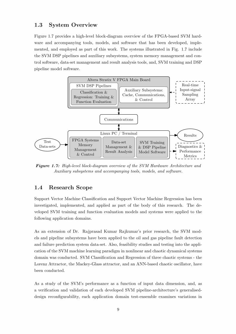
1.3 System Overview
Figure 1.7 provides a high-level block-diagram overview of the FPGA-based SVM hard-
ware and accompanying tools, models, and software that has been developed, imple-
mented, and employed as part of this work. The systems illustrated in Fig. 1.7 include
the SVM DSP pipelines and auxiliary subsystems, system memory management and con-
trol software, data-set management and result analysis tools, and, SVM training and DSP
pipeline model software.
Altera Stratix V FPGA Main Board
ResultsLinux PC / Terminal
TestData-sets Diagnostics &
PerformanceMetrics
Communications
FPGA SystemsMemory
Management& Control
Data-setManagement &Result Analysis
SVM Training& DSP PipelineModel Software
Auxiliary Subsystems:Cache, Communications,
& Control
Classification &Regression: Training &
Function Evaluation
SVM DSP Pipelines Real-timeInput-signal
SamplingArray
Figure 1.7: High-level block-diagram overview of the SVM Hardware Architecture andAuxiliary subsystems and accompanying tools, models, and software.
1.4 Research Scope
Support Vector Machine Classification and Support Vector Machine Regression has been
investigated, implemented, and applied as part of the body of this research. The de-
veloped SVM training and function evaluation models and systems were applied to the
following application domains.
As an extension of Dr. Rajprasad Kumar Rajkumar’s prior research, the SVM mod-
els and pipeline subsystems have been applied to the oil and gas pipeline fault detection
and failure prediction system data-set. Also, feasibility studies and testing into the appli-
cation of the SVM machine learning paradigm in nonlinear and chaotic dynamical systems
domain was conducted. SVM Classification and Regression of three chaotic systems - the
Lorenz Attractor, the Mackey-Glass attractor, and an ANN-based chaotic oscillator, have
been conducted.
As a study of the SVM’s performance as a function of input data dimension, and, as
a verification and validation of each developed SVM pipeline-architecture’s generalised-
design reconfigurability, each application domain test-ensemble examines variations in
9

data dimensionality through various techniques and mechanisms specific to its host do-
main.
In all application domains the SVM system’s primary performance metric is that of real-
time operation; all other metrics of interest, both technically quantitative and qualitative,
have been measured based principally upon the system’s real-time performance and secon-
darily informed by the specific application domain and its typical engineering constraints.
1.5 Subject Area Contributions
The scope of this work encompasses four subject areas; FPGA Hardware Design and
Implementation, Digital Signal Processing, Machine Learning, and Chaotic and Nonlinear
Systems. The Venn diagram in Fig. 1.8 illustrates this relationship, culminating with this
work’s tangible output, the SVM hardware architectures. This work incorporates elements
of, and in-turn contributes back to, these research subject areas.
SVMHardware
Architecture
ChaoticSystems
MachineLearning
FPGAHardwareDesign
DigitalSignal
Processing
Figure 1.8: Venn diagram illustrating the four subject areas covered in this work’sscope and its subsequent research contributions.
1.6 Organisation
This thesis is organised into the following chapters; Preface, Glossary, Chapter 1: In-
troduction, Chapter 2: Preliminaries, Chapter 3: Literature Review, Chapter 4: System
Architecture and Scientific Method, Chapter 5: Results, Chapter 6: Discussion, and
Chapter 7: Conclusion. Finally Appendices followed by References are found at the end
of this thesis.
A Table of Contents can be found at the beginning of this thesis and Appendices and
References can found at the end of this thesis.
10

The Preface contains a list of supporting publications derived from this work and lists of
all figures and tables found within this thesis. The Glossary contains a list of mathemat-
ical and scientific notation, and, a list of acronyms and abbreviations used throughout
this thesis.
Chapter 1 introduces the scope and goals of this research project.
Chapter 2 defines the fundamental concepts used and applied freely and frequently through-
out the thesis. These concepts are included in this chapter to alleviate clutter and thus
afford coherent development of new concepts, and, to serve as a convenient reference for
the reader.
Chapter 3 contains the most recent review of currently available literature pertaining
to the scope of currently completed work. It identifies gaps in the literature that have
been addressed, and, presents concepts imparted through the literature that have been
applied and extended throughout this body of work.
Chapter 4 describes the design and development of systems implemented throughout
this work, and, provides an overview of data-sets and the scientific method applied to test
these system implementations.
Chapter 5 presents technical specifications and measured data pertaining to the systems
designed and developed as part of this work, and, the results to the application of the
data-sets and scientific method described in the previous chapter.
Chapter 6 provides an extensive discussion of the system designs and implementations
presented in Chapter 4 and a discussion of the technical specifications, measured data,
and results presented in the Chapter 5.
Chapter 7 briefly summarises the research project objectives, goals, and outcomes and
thus concludes the thesis.
The Appendices contain a listing of all DSP instructions used in the developed SVM
pipelines and the VHDL entities of the prototyped SVM DSP pipelines.
Finally the References chapter contains a list, in the standard IEEE citation style, of
all publications and literature explicitly cited in this thesis.
11

Chapter 2
Preliminaries
This chapter defines the mathematical conventions, principles, and methods used through-
out the development of the SVM systems presented in this thesis. These conventions are
provided as a concise and succinct reference to mathematical operations and methods,
including nomenclature, utilised and developed in later chapters; both proofs and deriva-
tions have been omitted.
Support Vector Machine operation is composed of the multidimensional mathematics
of Linear Algebra. Section 2.1 provides an overview of this field of mathematics. Vector
and matrix conventions, vector space definitions, lines, planes, and hyperplanes theory,
concepts and nomenclature used throughout this thesis are covered.
SVM training is an optimisation problem. Thus optimisation problem theory and ac-
companying nomenclature are defined in Section 2.2.
Finally Section 2.3 Taylor Series and Section 2.4 are presented as they provide key func-
tional definitions and approximations useful for the implementation of SVM in digital
systems.
2.1 Linear Algebra
2.1.1 Vectors and Matrices
A vector is a one dimensional array of n elements, such as a data time series or a position
vector in Rn, and will be represented by a bar-accented bold-type lower-case Roman
or Greek character. E.g. vector x is a one dimensional column vector of n elements
{x1, x2, · · · , xn} in Rn and is defined as
x =
x1
x2
...
xn
, (2.1)
12

The cardinality of x, written |x|, is the number of elements in x, and is therefore n. The
transpose of x, a one dimensional row vector of n elements in Rn, represented as xT , is
defined as
xT =[x1 x2 · · · xn
]. (2.2)
Given vector x defines a position vector in Rn, the length of x, known as the norm and
represented by ‖x‖, is defined as
‖x‖ =√x • x. (2.3)
A matrix is a two dimensional array of m×n components, such as multi-sensor data time
series or an ANN connection weight matrix, and is represented by a bold-type upper-case
Roman or Greek character. E.g. A is a two dimensional matrix of m × n components
and is defined as
A =
a11 a12 · · · a1n
a21 a22 · · · a2n
......
. . ....
am1 am2 · · · amn
. (2.4)
If B is an n× n square matrix and is invertible, the inverse of matrix B, represented as
B−1, is defined as
BB−1 = I, (2.5)
where I is an n×n square matrix known as the identity matrix, with 1’s on the diagonal
and 0’s off the diagonal, defined as
I =
1 0 · · · 0
0 1 · · · 0...
.... . .
...
0 0 · · · 1
. (2.6)
2.1.2 Vector Spaces
A set of vectors v = v0, v1, · · ·, vk in Rn is called a vector space, or subspace, in Rn. The
vectors of set v are said to be linearly independent if there exist no scalar constants C1,
C0, · · ·, Ck that satisfy the dependence relation
v0 = C1v1 + · · ·+ Ckvk, (2.7)
that is, no vector can be expressed as a linear combination of the other vectors in the
set [30]. In this special case it is said that the span of the vectors v0, v1, · · ·, vk form a
basis for the subspace v within the space Rn. If the subset v forms the columns of matrix
V such that
V =[v0 v1 · · · vk
], (2.8)
13

then the columns of matrix V are also said to be linearly independent.
The dot product, or the inner product, of two column vectors x and y is defined as
x • y = xT y =n∑
i=1
xiyi = x1y1 + x2y2 + · · ·+ xnyn = ‖x‖‖y‖ cos γ, (2.9)
where γ is the angle between the two vectors [30]. The dot product of two identical vectors
is 1. The dot product of two orthogonal vectors is 0. A vector space where dot-products
are defined is referred to as a dot product space.
2.1.3 Lines, Planes, and Hyperplanes
Machine learning based systems, such as SVMs, are often employed to classify data into
separate and distinct classes. Examples of this will be presented in Chapter 3. One simple
and intuitive mechanism for classification of two distinct classes is to draw a straight line
through a set of data points and label the points according to whether they lie above or
below the line. This strategy also applies to higher dimensional data sets by employing a
plane or hyperplane in place of a line.
A straight line in R2 that crosses through the origin is defined as
mx1 + x2 = 0. (2.10)
Equation 2.10 can be rewritten as a dot product of vectors w = {m, 1} and x = {x1, x2}
w • x = 0. (2.11)
Interpreting Eq. 2.11 geometrically, vector x is a position vector for any point {x1, x2}that lies on, and is parallel to, the line w • x = 0 [31]. Vector w is known as the normal
vector and is orthogonal to the line w • x = 0, as shown in Fig. 2.1.
14

x2
x1
w • x = 0x1
x2
w
Figure 2.1: Line in R2 expressed as a dot product, w • x = 0, the orthogonal normalvector w, and two possible position vectors, x1 and x2, of which both lie on, and are
orthogonal to, the line.
Similarly, a straight line in R2 with an offset b is defined as
w • x = b. (2.12)
The normal vector w is still orthogonal to the line w • x = b, but is no longer orthogonal
to the position vector x. Figure 2.2 illustrates the introduction of the offset term b on
the the vectors w and x, and line itself.
x2
x1
w • x = bx1
x2
w
bw2
Figure 2.2: Line in R2 expressed as a dot product, w • x = b, the orthogonal normalvector w, and two possible position vectors, x1 and x2, of which both are points on the
line.
This theory can also be extended to apply to planes in R3 and hyperplanes in higher
dimensional cases of Rn [31]. Figure 2.3 shows a plane in R3 defined by the dot product
w • x = b.
15

x2 x1
w • x = bx1
x2
wx3
bw3
Figure 2.3: Plane in R3 expressed as a dot product, w • x = b, the orthogonal normalvector w, and two possible position vectors, x1 and x2, of which both are points on the
plane.
2.2 Optimisation Problems
Optimisation problems involve finding the best solution for some objective function φ :
Rn → R given some constraint hi : Rn → R with bound ci. An optimisation problem is
formally defined as
minxφ(x), (2.13)
such that
hi(x) ≥ ci, (2.14)
where i = 1, · · · , k for all x ∈ Rn. Any value x ∈ Rn that satisfies the constraints is called
a feasible solution. The optimisation aims to find the feasible solution x∗ that minimises
the objective function such that for any other feasible solution q ∈ Rn the equality
φ(x∗) ≤ φ(q) (2.15)
holds [32]. Optimisation problems are not limited to just objective function minimisation.
The following identities provide a mechanism to perform objective function maximisation:
maxφ(x) = |min−φ(x)|, (2.16)
maxφ(x) = min1
φ(x), (2.17)
provided 1/φ(x) is defined. An optimisation problem is linear when the associated ob-
jective function and constraints are linear. When either the objective function or the
constraints are not linear, the optimisation problem is non-linear.
The optimisation problems encountered in SVM training are non-linear and known specif-
ically as convex optimisation problems. A convex optimisation problem has a convex ob-
16

jective function and linear constraints. Consider the function f : R → R shown in Fig.
2.4. Let a, b ∈ R be any values such that a < b, and let g : R → R be a linear function
such that g(a) = f(a) and g(b) = f(b). The function f is said to be convex if f(x) ≤ g(x)
for all values x ∈ R such that a < x < b. For the convex function f , the line g can touch
the graph of the function for any interval [a, b] in R, but cannot cross it [31].
x
y
f(x)
g(x)
ba
f(a)
f(b)
Figure 2.4: The linear function g(x) intersects the convex function f(x) at points(a, f(a)) and (b, f(b)).
One method of solving convex optimisation problems is via quadratic programming.
2.3 Taylor Series
It is often computationally necessary to express known functions as an infinite series
known as a power series. A Taylor series is an infinite sum approximation of a function
with terms calculated from the function’s derivatives at a single point. For example the
exponential function ex can be expressed as the power series
ex =∞∑
n=0
xn
n!= 1 + x+
x2
2!+x3
3!+x4
4!+ · · · , (2.18)
and, the hyperbolic tangent function tanh(x) can be approximated by the Taylor series
tanh(x) = x− x3
3+
2x5
15− 17x7
315+ · · · , |x| < π
2. (2.19)
2.4 State-Space Methods
State-Space methods provide a powerful time-domain mechanism, as opposed to classical
Laplacian frequency-domain techniques, for the design and analysis of digital systems and
the dataspaces the multidimentional mathematics occupy. State-space methods exploit
multidimensional mathematics of linear algebra. Thus the analysis of both Single-Input-
Single-Output, Multiple-Input-Single-Output, and Multiple-Input-Multiple-Output sys-
tems with many free variables is easily undertaken, manageable, and well suited to digital
17

and computational investigation, analysis, and control [33].
The state-space of some system, with p inputs, q outputs, and n state variables, is defined
by the following two equations
˙x = Ax+Bu, (2.20)
y = Cx+Du, (2.21)
where x ∈ Rn is the state vector, y ∈ Rq is the output vector, u ∈ Rp is the input vector,
A is the n× n state matrix, B is the n× p input matrix, C is the q × n output matrix,
D is a q×p matrix and is known as the feedforward matrix, and ˙x ∈ Rn is the next-state
vector [34]. The state matrix A is a matrix representation of the system of differential
equations or difference equations that describe the given system’s dynamics. Knowing the
entire state of a system x at some time, and if the system’s dynamics A are also known,
the complete set of all states of the system’s response can be computed for some input
u. By modifying the B and D matrices accordingly some desired form of system control
can also be implemented [35].
The Gradient ∇ [36], [37] is a calculus-based tool useful for determining properties of
some state-space, described by the state matrix A, and of specific regions of state-space,
identified by points defined by the state vector and next state vector x and ˙x respectively.
The Gradient ∇ of state matrix A column Ai is the n × 1 column-vector of first-order
partial derivatives of the time-evolution function described by column Ai with respect to
x, thus
∇xAi = ∇Ai =∂Ai∂x
=
[∂Ai∂x1
· · · ∂Ai∂xn
]. (2.22)
18

Chapter 3
Literature Review
This chapter provides a summary of the core texts pertaining to the scope of this work.
It provides a complete overview of all relevant texts considered as part of this research
work. This chapter identifies key concepts and gaps in the literature that this research
work aims to address, supplement, and extend where appropriate.
The chapter is organised into the three sections; Machine Learning with Support Vec-
tor Machines, Digital Signal Processing and Altera Stratix V FPGA, and finally, Chaotic
and Nonlinear Systems.
3.1 Machine Learning with Support Vector Machines
Machine learning as a field is a very vast and complex one; to provide even an overview
of all machine learning paradigms would require one very large volume, if not more,
just to introduce the core fundamentals of each. With this in mind, this section has
been written with the intend in providing only the concepts pertaining to Support Vector
Machines explicitly, and where appropriate, the theories and literature that provide a solid
foundation for the continued research and development towards implementing a real-time
hardware-based SVM system.
3.1.1 Maximum-Margin Classifiers and SVMs
Considerable work has gone into SVM research and development, and a clear evolution
of the paradigm can be observed in the literature. This subsection introduces the SVM
paradigm from the its Maximum-Margin Classifiers ancestry through to Vapnik’s influ-
ential and relevant theory of statistical-based machine learning and the SVMs advanced
learning, classifying, and regression applications.
3.1.1.1 Maximum-Margin Classifiers
Before providing an exposition of the Maximum-Margin Classifier paradigm, several re-
lated concepts require formal definition. In binary classification problems a hyperplane
supports a class of data-points if it is parallel to a linear decision surface and all points
19

of its respective class are either above or below it. Such a hyperplane is referred to as
a supporting hyperplane. The distance between the two supporting hyperplanes is called
a margin. A decision surface is optimal if it is equidistant from the two supporting hy-
perplanes and maximises their margin [31]. Figure 3.1 provides an illustration of these
concepts in R2.
Margin
Class +1
Class −1
Support Vectors
Support Vectors
SupportingHyperplanes
OptimalDecision Surface
Figure 3.1: Optimal decision surface with its two supporting hyperplanes separatingtwo linearly separable classes.
Given a linearly separable training data set D
D = {(x1, y1), (x2, y2), · · · , (xk, yk)} ⊆ Rn × {+1,−1}, (3.1)
one can compute a maximum-margin decision surface w∗ • x = b∗ with the optimisation
minφ(w, b) = minw,b
12w • w (3.2)
subject to the constraints
w • (yixi) ≥ 1 + yib for all (xi, yi) ∈ D. (3.3)
Figure 3.2 illustrates an example of a maximum-margin class separation of some arbitrary
linearly separable data set in R2 by an optimal decision surface w∗•x = b∗. Corresponding
supporting hyperplanes are separated by an optimal margin and are both equidistant from
the optimal decision surface.
20
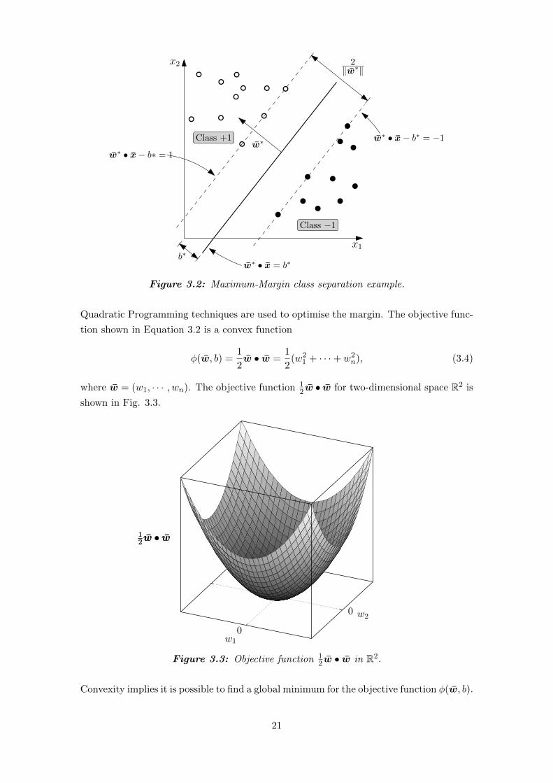
b∗
w∗ w∗ • x− b∗ = −1w∗ • x− b∗ = 1
w∗ • x = b∗
2‖w∗‖
x1
x2
Class +1
Class −1
Figure 3.2: Maximum-Margin class separation example.
Quadratic Programming techniques are used to optimise the margin. The objective func-
tion shown in Equation 3.2 is a convex function
φ(w, b) =1
2w • w =
1
2(w2
1 + · · ·+ w2n), (3.4)
where w = (w1, · · · , wn). The objective function 12w • w for two-dimensional space R2 is
shown in Fig. 3.3.
0
0
12w • w
w1
w2
12w • w
Figure 3.3: Objective function 12w • w in R2.
Convexity implies it is possible to find a global minimum for the objective function φ(w, b).
21
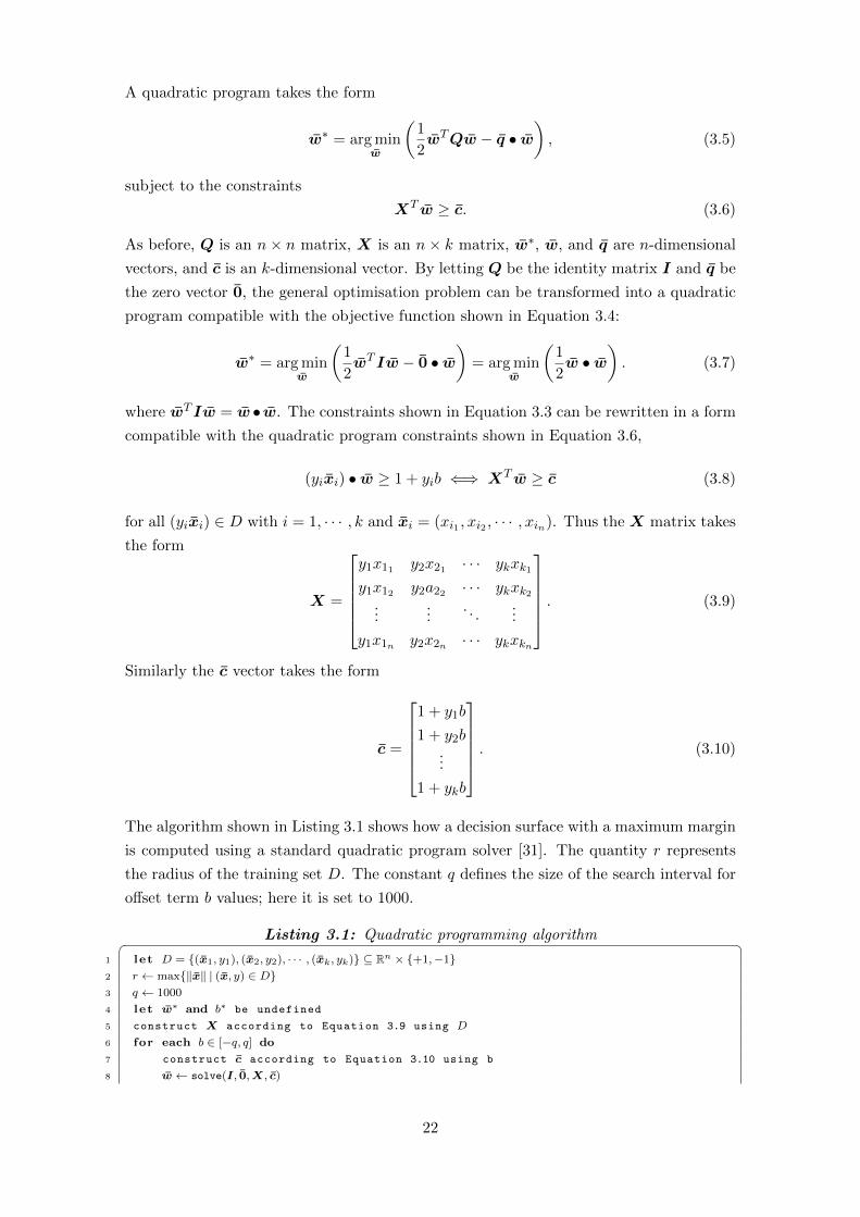
A quadratic program takes the form
w∗ = arg minw
(1
2wTQw − q • w
), (3.5)
subject to the constraints
XT w ≥ c. (3.6)
As before, Q is an n× n matrix, X is an n× k matrix, w∗, w, and q are n-dimensional
vectors, and c is an k-dimensional vector. By letting Q be the identity matrix I and q be
the zero vector 0, the general optimisation problem can be transformed into a quadratic
program compatible with the objective function shown in Equation 3.4:
w∗ = arg minw
(1
2wT Iw − 0 • w
)= arg min
w
(1
2w • w
). (3.7)
where wT Iw = w • w. The constraints shown in Equation 3.3 can be rewritten in a form
compatible with the quadratic program constraints shown in Equation 3.6,
(yixi) • w ≥ 1 + yib ⇐⇒ XT w ≥ c (3.8)
for all (yixi) ∈ D with i = 1, · · · , k and xi = (xi1 , xi2 , · · · , xin). Thus the X matrix takes
the form
X =
y1x11 y2x21 · · · ykxk1y1x12 y2a22 · · · ykxk2
......
. . ....
y1x1n y2x2n · · · ykxkn
. (3.9)
Similarly the c vector takes the form
c =
1 + y1b
1 + y2b...
1 + ykb
. (3.10)
The algorithm shown in Listing 3.1 shows how a decision surface with a maximum margin
is computed using a standard quadratic program solver [31]. The quantity r represents
the radius of the training set D. The constant q defines the size of the search interval for
offset term b values; here it is set to 1000.
Listing 3.1: Quadratic programming algorithm� �1 let D = {(x1, y1), (x2, y2), · · · , (xk, yk)} ⊆ Rn × {+1,−1}2 r ← max{‖x‖ | (x, y) ∈ D}3 q ← 1000
4 let w∗ and b∗ be undefined
5 construct X according to Equation 3.9 using D
6 for each b ∈ [−q, q] do
7 construct c according to Equation 3.10 using b
8 w ← solve(I, 0,X, c)
22

9 i f (w is defined and w∗ is undefined) or (w is defined and ‖w‖ < ‖w∗‖) then
10 w∗ ← w
11 b∗ ← b
12 end i f
13 end for
14 i f w∗ is undefined then
15 stop constraints not satisfiable
16 else i f ‖w∗‖ > q/r then
17 stop bounding assumption of ‖w‖ violated
18 end i f
19 return (w∗, b∗)� �3.1.1.2 Support Vector Machine Classifiers
A Support Vector Machine (SVM) is the optimisation of the Lagrangian dual of the
Maximum-Margin Classifier. Consider the Lagrangian L(α, x) defined as
L(α, x) =1
2x2 − α(x− 2). (3.11)
Therefore the optimisation of the Lagrangian convex objective function L(α, x), as shown
in Fig. 3.4 in R2, is a unique saddle-point on L(α, x).
0
0
L(α, x)
α
x
L(α, x)
Figure 3.4: Lagrangian objective function L(α, x) = 12x
2 − α(x− 2) in R2.
The optimal unique saddle point on the Lagrangian L(α, x) has to occur where the the
gradient of L(α, x) with respect to x is equal to zero:
∂L(α, x∗)∂x∗
= x∗ − α = 0 (3.12)
where x∗ represents the value that minimises the Lagrangian with respect to x at the
saddle-point. Solving for x∗ and substituting into Eq. 3.11 gives the Lagrangian dual
23

optimisation with φ′(α) = L(α, x∗),
arg maxα
φ′(α) = arg maxα
(2α− 1
2α2
)(3.13)
subject to
α =≥ 0. (3.14)
The derivation of the maximum-margin classifier Lagrangian dual optimisation problem,
the SVM, follows. Recall the maximum-margin optimisation problem
arg minw,b
φ(w, b) = arg minw,b
(1
2w • w
)(3.15)
subject to the constraints
gi(w, b) = yi(w • xi − b)− 1 ≥ 0 (3.16)
for i = 1, · · · , k. The corresponding Lagrangian is constructed
L(α, w, b) = φ(w, b)−k∑
i=1
αigi(w, b)
=1
2w • w −
k∑
i=1
αi(yi(w • xi − b)− 1)
=1
2w • w −
k∑
i=1
αiyiw • xi + bk∑
i=1
αiyi +k∑
i=1
αi.
(3.17)
Thus the Lagrangian optimisation problem for maximum-margin classifiers is given by
maxα
minw,b
L(α, w, b), (3.18)
subject to
αi =≥ 0. (3.19)
for i = 1, · · · , k. Let α∗, w∗, and b∗ be a solution to the Lagrangian optimisation problem
such that
maxα
minw,b
L(α, w, b) = L(α∗, w∗, b∗), (3.20)
Since φ is convex and the constraints gi are linear, the solution α∗, w∗, and b∗ will satisfy
24

the following Karush-Kuhn-Tucker (KKT) conditions:
∂L(α∗, w∗, b∗)∂w
= 0, (3.21)
∂L(α∗, w∗, b∗)∂b
= 0, (3.22)
α∗i (yi(w∗ • xi − b∗)− 1) = 0, (3.23)
yi(w∗ • xi − b∗)− 1 ≥ 0, (3.24)
α∗i ≥ 0 (3.25)
for i = 1, · · · , k. By taking the partial derivatives of the Lagrangian defined in Eq. 3.17
with respect to w and b, setting each to zero as defined in the KKT conditions defined
in Eq. 3.21 and Eq. 3.22, and substituting back into Eq. 3.17 the Lagrangian dual for
maximum-margin classifiers can be constructed
φ′(α) = L(α, w∗, b∗) =k∑
i=1
αi −1
2
k∑
i=1
k∑
j=1
αiαjyiyjxi • xj . (3.26)
Thus the SVM is defined as follows. Given a labelled linearly separable training data set
D defined as
D = {(x1, y1), (x2, y2), · · · , (xk, yk)} ⊆ Rn × {+1,−1}, (3.27)
where yi = f(xi) and f is some target function where f : Rn → {+1,−1}, one can
compute a model f : Rn → {+1,−1} using D such that
f(x) ∼= f(x) (3.28)
for all x ∈ Rn. Therefore support vector models are trained with the dual Lagrangian
optimisation for maximum-margin classifiers
α∗ = arg maxα
k∑
i=1
αi −1
2
k∑
i=1
k∑
j=1
αiαjyiyjxi • xj
, (3.29)
subject to the constraints
k∑
i=1
αiyi = 0, and (3.30)
αi ≥ 0, (3.31)
where α = {α1, α2, · · · , αk} are Lagrangian multipliers and i = 1, · · · , k. Data points
with non-zero Lagrangian multipliers are called support vectors xsv.
25

The model f(x) is defined as the linear support vector machine
f(x) = sgn
(k∑
i=1
α∗i yixi • x−k∑
i=1
α∗i yixi • xsv+ + 1
), (3.32)
where one support vector xsv+ is chosen from from the set of available support vectors,
(xsv+ ,+1) ∈ {(xi,+1) | (xi,+1) ∈ D and α∗i > 0}. (3.33)
In practice data sets are rarely linearly separable. This can be overcome by the application
of kernel functions. An appropriately chosen kernel function will transform the input space
where the data set is is not linearly separable to a higher-dimensional space called a feature
space where the data set is linearly separable. Conversely this kernel function mapping
transforms a nonlinear decision problem in the input space into a linear decision problem
in the feature space. Also by choosing the right kernel function all calculations can be
performed in the input space, implying that the act of performing the transformations is
completely avoided, thus so too is any computational cost incurred by the transformations.
This is called the kernel trick. Let Φ : Rn → Rn be the identity function on Rn, then the
kernel function ψ can be defined as
ψ(x, y) = Φ(x) • Φ(y) = x • y, (3.34)
where x, y ∈ Rn. This is the linear kernel, and the feature space is the same as the input
space. The support vector models can now be trained by rewriting Equation 3.29 and
optimising the Lagrangian
α∗ = arg maxα
k∑
i=1
αi −1
2
k∑
i=1
k∑
j=1
αiαjyiyjψ(xi, xj)
, (3.35)
subject to the same constraints given in Equations 3.30 and 3.31. Likewise the linear
support vector machine model f(x) can be redefined as
f(x) = sgn
(k∑
i=1
α∗i yiψ(xi, x)−k∑
i=1
α∗i yiψ(xi, xsv+) + 1
). (3.36)
There exist many nonlinear kernel functions ψ that can be substituted into Equations
3.35 and 3.36 allowing the effective transformation of data sets from the input space to
the feature space while maintaining the computation benefits of the kernel trick. Table
3.1 presents some commonly used kernel functions.
26

Table 3.1: Commonly used kernel functions and their free parameters.
Kernel NameKernel Function ψ(x, y),
x, y ∈ RnFree
Parameters
Linear Kernel ψ(x, y) = x • y noneHomogeneous Polynomial Kernel ψ(x, y) = (x • y)d d ≥ 2
Nonhomogeneous Polynomial Kernel ψ(x, y) = (x • y + c)d d ≥ 2, c > 0
Gaussian Kernel ψ(x, y) = e−(‖x−y‖2/2σ2) σ > 0
Radial Basis Function (RBF) Kernel ψ(x, y) = e−(γ‖x−y‖2) γ > 0
Sigmoid / Hyperbolic Tangent Kernel ψ(x, y) = tanh(x • y + c) c > 0
Real world data sets will also always contain some form of noise. To mitigate the effects
of noisy datasets it is prudent to allow the training of an SVM to make mistakes. Al-
lowing the training algorithm to ignore certain points in a data set, points that may be
discoloured by some noise present in the data, gives rise to much simpler decision surfaces,
and consequently, decision surfaces that tend to generalise better.
To reduce the impact of noisy training data the introduction of slack variables ξj al-
low troublesome points to lie on the wrong side of their respective supporting hyperplane.
The slack variables measure how much error is committed by allowing the supporting hy-
perplane to be unconstrained by that point [31]. Classifiers that employ slack variables in
this manner are known Soft-margin classifiers. Soft-margin class separation is illustrated
in Fig. 3.5. An upper bound on the compounded error conceded by non-zero erroneous
slack variables is defined as
C∑
j
ξj , (3.37)
where C is called the cost. A soft-margin SVM classifier can be derived by developing
the Lagrangian dual of the maximum-margin classifier with the term defined in Equation
3.37 added to the primal objective function Lagrangian. The cost term C only appears in
the Lagrangian dual optimisation constraints. The cost C controls the trade-off between
margin-size and classification error. A larger cost C forces the optimisation to permit
fewer non-zero erroneous slack variables, therefore a smaller margin will be found, thus
increasing the cost in both complexity and potentially-lost generalisation ability.
27

w
w • x− b = −1
w • x− b = 1
w • x = b
x1
x2
Class +1
Class −1
xj
ξj
Figure 3.5: Soft-Margin Classifier class separation example.
The soft-margin support vector models can now be trained by optimising the Lagrangian
α∗ = arg maxα
k∑
i=1
αi −1
2
k∑
i=1
k∑
j=1
αiαjyiyjψ(xi, xj)
, (3.38)
subject to the modified constraints
k∑
i=1
αiyi = 0, and (3.39)
C ≥ αi ≥ 0, (3.40)
where i = 1, · · · , k and C is the cost constant.
As before the support vector machine model f(x) is defined as
f(x) = sgn
(k∑
i=1
α∗i yiψ(xi, x)−k∑
i=1
α∗i yiψ(xi, xsv+) + 1
), (3.41)
however, one must be careful to choose a support vector xsv+ with a zero valued slack
variable ξ∗sv+ = 0 from the set of available support vectors,
(xsv+ ,+1) ∈ {(xi,+1) | (xi,+1) ∈ D and 0 < α∗i < C}. (3.42)
3.1.1.3 Statistical Learning Theory
Initially developed by Vladimir Naumovich Vapnik and Alexey Jakovlevich Chervonenkis,
Statistical Learning Theory, or VC-Theory, provides the theoretical foundation that the
SVM machine learning paradigm is based. At the core of this theoretical foundation lies
28

the model of learning from examples, as shown in Fig. 3.6 [26]- [28]. The model consists
of three distinct elements; a random process of some unknown probability distribution
P (x) = P (x, y), a supervisor, and a learning machine.
SupervisorP (y | x)
Learning Machinew ∈W
RandomProcess with UnknownProbability Distribution
P (x)X = x0, x1, · · · , xk
X ∈ Rn
(X, y) =(x0, y0), (x1, y1), · · · , (xk, yk)
f(x, w) = y
xi
Figure 3.6: Statistical Learning Theory: The model of learning from examples.
The random process P (x) generates independent and identically distributed (i.i.d.) data
vectors x0, · · · , xk = X that serve as the input to the supervisor. The supervisor de-
termines a label yi ∈ {−1,+1} for each vector xi according to some unknown but fixed
decision function P (y | x). The labelled data pairs (X, y) serve as training data to the
learning machine. Given training data, the learning machine must choose a decision func-
tion f from the set of functions F (x, w), w ∈W that best approximates the supervisor’s
decision function, and thus correctly predict the response yi given any vector xi generated
by the random process. This is called the problem of learning.
Determining the decision function or model f ∈ F (x, w) that best approximates the
supervisor’s unknown decision function is achieved by minimising the difference between
the expected outputs yi and the response from the learning machine f(x, w), known as
the loss function L(y, f(x, w)). The loss function compares training data labels and model
f output labels; if the model performs a classification error on a data point xi the loss
function returns a 1, otherwise it returns a 0. The loss function is defined as
L(y, f(x, w)) =
{0 if y = f(x, w),
1 if y 6= f(x, w).(3.43)
The expected loss or the expected risk of some function f ∈ F (x, w) over the entire
data-space is defined as
R[f ] = E[L(y, f(x, w))] =
∫L(y, f(x, w))dP (x, y). (3.44)
Thus minimising the expected risk finds the best generalisation of the supervisor’s decision
function, the optimal learning machine model f∗,
29

f∗ = arg minf∈F (x,w)
R[f ], (3.45)
and appears to solve the problem of learning [31]. However the joint probability distri-
bution P (x, y) is unknown, thus Eq. 3.45 is of no practical usefulness or benefit. The
joint probability distribution of the observed training data, however, is known. The risk
estimated using the training data is called the empirical risk Remp[f ] of some model f ,
and is defined as
Remp[f ] = E[L(y, f(x, w))] =1
k
k−1∑
i=0
L(yi, f(xi, w)), (3.46)
where (xi, yi) ∈ (X, y). Thus by minimising the empirical risk, known as Empirical Risk
Minimisation, the optimal learning machine model f∗ can be calculated;
f∗ = arg minf∈F (x,w)
Remp[f ]. (3.47)
Minimising the empirical risk Remp[f ] and finding the optimum model f∗ from the set of
all functions F (x, w) has the upshot of defining a model that will exhibit a risk Remp[f ]
or classification error of effectively zero for the training data. The caveat to this situation
however is the optimal model f∗ does not generalise the supervisor’s decision function
well, and the model will exhibit data overfitting when new unseen unlabelled data is clas-
sified. This will be observed as an increase in the risk Remp[f ] as classification errors.
To overcome this drawback of the Empirical Risk Minimisation (ERM), Vapnik devel-
oped the concept of Structural Risk Minimisation. Structural Risk Minimisation (SRM)
utilises the concept of classifier model complexity, known as the VC-dimension h, for a
given training data set [38], [39]; the VC-dimension of a model class is data dependent [31].
The VC-dimension is a measure of how well a binary classifier can model the boundary
between two classes; the larger the VC-dimension, the more complex the classifier, and,
the better it can separate the data into its two respective classes.
The formal definition of a classifier’s VC-dimesion follows. Let F [γ] denote a class of
linear classifiers all with the same margin size γ. Assume that the model class F [γ] is
closed under rotation and translation, or, for all f ∈ F [γ], all rotations ρ and all trans-
lations τ have ρ(f) ∈ F [γ] and τ(f) ∈ F [γ]. The VC-dimension of a model class F [γ]
defined over some data set D is the size of the largest finite subset of D shattered by F [γ].
The following exposition and Fig. 3.7 provides an elaboration and visual illustration
respectively of the VC-dimension for two classifier model classes, F [γ1] and F [γ2], over a
small three-vector data set D ⊂ R2. Let the two distinct classes of classifiers F [γ1] and
F [γ2] be defined over D. The margin γ1 is chosen such that the classifier model class can
separate all three instances for all possible binary label assignments, as shown in Fig. 3.7
30

(a). In this instance the VC-dimension of F [γ1] is 3, or, h1 = 3. Since the VC-dimension
h1 is equal to the dimension of the data set, it is said that F [γ1] shatters D. The margin
γ2 is chosen such that γ2 > γ1, and so that the class of classifiers F [γ2] cannot separate
all instances perfectly, as shown in Fig. 3.7 (b). However, if the grey instance in Fig.
3.7 (b) is removed, the classifiers in F [γ2] can shatter this subset of D. Therefore the
VC-dimension for the model class F [γ2] is 2, or h2 = 2. As h1 > h2 it is said the classifiers
in F [γ1] are more complex than the classifiers in F [γ2], or, F [γ1] ⊃ F [γ2] [31].
(a) (b)
γ1
γ1
γ1
γ1
γ1
γ1
γ1
γ1
γ2
γ2
γ2
γ2
γ2
γ2
γ2
γ2
Figure 3.7: Illustration of the VC-dimension h of two classifiers F [γ1] and F [γ2] ofdecreasing complexity on an arbitrary data-set D; (a) classifier F [γ1] with margin γ1
shatters D, thus hγ1 = 3, and (b) classifier F [γ2] with margin γ2 shatters only two datapoints, thus hγ2 = 2.
The preceding example illustrated the VC-dimension of two linear model classes, however
the theoretical development shown here can be extended to include nonlinear decision
surfaces for any kernel function, as well as soft-margin classifiers. It should be noted that
classifier model class complexity is not only dependant on the margin, but also influenced
31

by the cost constant and the type of kernel used in the model class.
Using the VC-dimension h, the VC-confidence υ(k, h, η), a measure of the generalisa-
tion error of a model based upon its VC-dimension, can be calculated. It is defined
as
υ(k, h, η) =
√h(log(2k
h ) + 1)− log(η4 )
k, (3.48)
where k is the size of the training data, h is the VC-dimension of the classifier model, and
η is the learning rate of the classier such that 0 < η < 1. Thus the upper error bound,
the generalisation error R[f ] or the generalisation bound, is defined as
R[f ] ≤ Remp[f ] + υ(k, h, η), (3.49)
Therefore given the empirical risk and the VC-confidence of the model, one can estimate
an upper bound on the expected loss of the model over the entire underlying data universe
[31]. Vapnik has shown that this upper bound holds with a probability of 1 − η. Figure
3.8 illustrates the relationship between the empirical risk Remp[f ] and the VC-confidence
υ(k, h, η).
υ(k, h, η)
Error
Remp[f ]
Function / Model Complexity
Generalisation Bound
f∗
Figure 3.8: Structural Risk Minimisation.
Minimising the generalisation bound is equivalent to making the right trade-off between
model complexity and generalisation error, and thus will give the optimal classifier model
f∗. Thus the process of Structural Risk Minimisation entails solving the optimisation
problem to find the optimal classifier model f∗,
f∗ = arg minf∈F
(Remp[f ] + υ(k, h, η)
), (3.50)
where F is the superclass of all model classes.
32

3.1.1.4 SVM Training and Optimisation Techniques
Vapnik proposes a method to solve the SVM Quadratic Programming (QP) problem
that has since become known as Chunking [40]. Vapnik’s chunking algorithm involves
iteratively removing rows and columns of the matrix Q, each corresponding to zero-
valued Lagrange multipliers, where Q is composed of elements qij = yiyjψ(xi, xj). By
optimising only a small sub-set of matrix Q each iteration, chunking reduces a large QP
problem into a series of smaller QP sub-problems where each iteration is initialised with
the results of the previous QP sub-problem [39]. Vapnik defines an SVM as trained when
the QP problem defined in Eq. 3.38, Eq. 3.39, and Eq. 3.40 is solved; an optimal feasible
point is found that satisfies the KKT conditions and the matrix Q composed of elements
qij = yiyjψ(xi, xj) is positive semi-definite. The KKT conditions are defined, for all i, as
αi = 0 ⇒ yi(w • xi − b) ≥ 1, (3.51)
0 < αi < C ⇒ yi(w • xi − b) = 1, (3.52)
αi = C ⇒ yi(w • xi − b) ≤ 1, (3.53)
Osuna et-al propose an extension of Vapnik’s chunking technique called the QP Decompo-
sition Algorithm [41]. By adding at least one example that violates the KKT conditions,
thus identifying a zero-valued Lagrange multiplier, to each QP sub-problem iteration,
the overall objective function maintains a feasible point that obeys all optimisation con-
straints, and, the sequence of QP sub-problems asymptotically converge [40]. Osuna’s
decomposition algorithm suggests maintaining a constant-sized matrix for each QP sub-
problem, thus granting deterministic resource consumption and arbitrarily sized data
sets [41].
Platt presents an algorithm for SVM training called Sequential Minimal Optimisation
(SMO) that out-performs both Vapnik’s chunking technique and Osuna et-al’s QP de-
composition algorithm [40]. Like chunking and Osuna’s decomposition method, SMO
decomposes the overall QP problem into smaller QP sub-problems [40]. SMO is moti-
vated by the principle dictated by the optimisation constraint
k∑
i=1
αiyi = 0, (3.54)
that is, αi values must be simultaneously updated in pairs in order to conform to this
constraint. The SMO algorithm is presented in Listing 3.2.
Listing 3.2: Sequential Minimal Optimisation algorithm� �1 while KKT conditions exceeded by convergence tolerance τ do
2 select αi and αj to update using some heuristic
3 optimise objective function φ(α) with respect to αi and αj while holding
αk(k 6= i, j) values fixed
4 end while� �33

Cichocki and Unbehauen [37] present a series of ANN-mapped techniques for the opti-
misation of nonlinear minimisation with mixed equality and inequality constraints. By
utilising exterior penalty function and interior penalty / barrier function methods the
constrained problem is approximated by an unconstrained minimisation problem. Opti-
misation of the unconstrained minimisation problem can then be accomplished using a
standard gradient descent algorithm, and the derived system of differential equations can
be mapped onto an ANN structure.
A constrained minimisation problem with mixed equality and inequality constraints is
defined as follows. Find x = [x1, · · · , xn]T ∈ Rn which minimises the scalar objective
function
f(x) = f(x1, · · · , xn) (3.55)
subject to the constraints
hi(x) = 0 (i = 1, · · · , p) and (3.56)
gi(x) ≥ 0 (i = p+ 1, · · · ,m). (3.57)
According to the extended interior approach the constrained optimisation problem shown
in Eq. 3.55 , Eq. 3.56, and Eq. 3.57 can be converted into an unconstrained minimisation
problem by constructing an energy function of the form
E(x, κ) = f(x) +
p∑
i=1
κih2i (x) +
m∑
i=p+1
1
κiBi(x), (3.58)
where κi > 0 and Bi(x) is the extended barrier function. The extended barrier function
is defined as
Bi(x) =
1
gi(x), if gi(x) ≥ ε,
2ε− gi(x)
ε2, if gi(x) < ε,
(3.59)
where ε is a small positive number which determines the transition from the exterior ex-
tended penalty to the interior penalty 1/gi(x).
By employing the dynamic gradient system, thus applying standard gradient descent
technique, a system of differential equations can be constructed and the local minimum
of the energy function shown in Eq. 3.58 can be found:
dx
dt= −µ∇xE(x, κ), (3.60)
where µ = diag(µ1, · · · , µn) and with the initial conditions x(0) = x(0). Thus
dxjdt
= −µj(∂f(x)
∂xj+
p∑
i=1
κihi(x)∂hi(x)
∂xj+
m∑
i=p+1
1
κi
∂Bi(x)
∂xj
), xj(0) = x
(0)j (3.61)
34

where µj > 0 for all j and κ ≥ 0. Typically µj = µ = 1/τ for all j where τ is the
integration time constant, and κi = κ for all i.
As the standard gradient descent algorithm will likely convergence to a local minima
rather than the desired global minimum, noise can be added to the system resulting in
a stochastic gradient descent technique [37]. By adding uncorrelated white noise to the
system of differential equations,
dx
dt= −µ∇xE(x, κ) + ν(t), (3.62)
where ν(t) is a vector of uncorrelated white noise sources with zero mean and variance
decreasing in time, the process becomes stochastic and thus the likelihood of convergence
to the desired global minimum is increased [37].
An ANN for convex Quadratic Programming is also presented by Cichocki and Unbe-
hauen [37] called the Augmented Lagrange Multiplier method, a combination of both
penalty function and ordinary Lagrange function optimisation techniques. The method
is presented as follows:
f(x) = f(x1, · · · , xn) (3.63)
subject to the constraints
hi(x) = 0 (i = 1, · · · , p) and (3.64)
gi(x) ≥ 0 (i = p+ 1, · · · ,m). (3.65)
The general augmented Lagrangian is then formed:
L(x, λ, κ) = f(x) +
p∑
i=1
(λihi(x) +
κi2h2i (x)
)+
m∑
i=p+1
(λig′i(x) +
κi2g′2i (x)
)(3.66)
where
g′i(x) =
gi(x), if gi(x) < −λiκi,
−λiκi, if gi(x) ≥ −λi
κi,
(i = p+ 1, · · · ,m). (3.67)
and κi ≥ 0 are the penalty parameters. The minimisation of the augmented Lagrangian
can be converted into a system of differential equations
dx
dt= −µ∇xL(x, λ, κ), (3.68)
dλ
dt= ρ∇λL(x, λ, κ), (3.69)
where µ = diag(µ1, · · · , µn) and ρ = diag(ρ1, · · · , ρm) are positive scalar variables, typ-
ically chosen as µi > 0 and ρi > 0, and with the initial conditions x(0) = x(0) and
35

λ(0) = λ(0)
. Thus
dxjdt
= −µj(∂f(x)
∂xj+
p∑
i=1
(λi∂hi(x)
∂xj+κi2hi(x)
∂hi(x)
∂xj
)
+m∑
i=p+1
(λi∂g′i(x)
∂xj+κi2g′i(x)
∂g′i(x)
∂xj
), xj(0) = x
(0)j , (3.70)
and
dλjdt
= ρj
(∂f(x)
∂λj+
p∑
i=1
(λi∂hi(x)
∂λj+κi2hi(x)
∂hi(x)
∂λj
)
+
m∑
i=p+1
(λi∂g′i(x)
∂λj+κi2g′i(x)
∂g′i(x)
∂λj
), λj(0) = λ
(0)j , (3.71)
As this is again the standard gradient descent algorithm, convergence to a local minima,
rather than the desired global minimum, is likely [37]. By adding uncorrelated white noise
to the system of differential equations,
dx
dt= −µ∇xL(x, λ, κ) + ν1(t), (3.72)
dλ
dt= ρ∇λL(x, λ, κ) + ν2(t), (3.73)
where ν1(t) and ν2(t) are vectors of uncorrelated white noise sources with zero mean and
variance decreasing in time, the process becomes stochastic and thus the likelihood of
convergence to the desired global minimum is increased [37].
Larsdon et-al present another technique for solving constrained nonlinear programming
problems called the Generalised Reduced Gradient, or GRG, algorithm [42] [43]. The Algo-
rithm is also known as the Conditional Gradient or Convex Combination search method,
and as Frank-Wolfe algorithm for projection-free sparse convex optimization [44]. The
problem defined as
minx∈D
f(x), (3.74)
where the objective function f(x) is convex and continuously differentiable and D is the
feasible compact convex set of some bounded vector space, can be solved by applying the
Frank-Wolfe algorithm shown in Listing 3.3.
Listing 3.3: Frank-Wolfe algorithm� �1 let x0 ∈ D2 for k = 0, · · · ,K do
3 find sk by solving arg min(sTk∇f(xk)) subject to sk ∈ D4 let γ = 2/(k + 2) or find γ by solving arg min(f(xk + γ(sk − xk))) subject to 0 ≤ γ ≤ 1
5 let xk+1 = xk + γ(sk − xk)
6 end for� �The Frank-Wolfe algorithm is regarded for both scalability and resultant solutions’ sparse
36

and low-rank properties [44].
Gilbert proposes an algorithm for finding a point which is closest to the origin for some
convex hull [45]. Gilbert’s algorithm has the advantages of ease-of-implementation on
general-purpose computing devices and can be analysed in a geometric manner, however,
has the disadvantage of exhibiting a decreasing rate of convergence as a solution is ap-
proached, referred to as vibration [46]. An improved Gilbert’s algorithm, with improved
vibration related convergence-rate decreases, is presented by Chang et-al [46]; Chang et-
al’s Improved Gilbert’s Algorithm is defined as follows. Let {zi}s1i=1 and {zi}s2i=1 be finite
point sets in Rn, U and V denote two convex polytopes, where
U = {u =
s1∑
i=1
αizi | αi ≥ 0,
s1∑
i=1
αi = 1}, (3.75)
and
V = {v =
s2∑
i=1
αizi | αi ≥ 0,
s2∑
i=1
αi = 1}. (3.76)
The aim of a general nearest point problem is to find the nearest points between the two
polytopes,
minu∈U,v∈V
‖u− v‖. (3.77)
Gilbert’s algorithm transforms the nearest point problem into one which finds the minimal
distance from the origin to a polytope. The Minkowski set difference of U and V is denoted
Z = U − V , thus Z is a polytope which has s1 × s2 vertices. It follows that the nearest
point problem is now the minimum distance problem:
minz∈Z‖z‖. (3.78)
The mathematical notation of the support properties of a convex polytope are presented
below. Suppose P is a convex polytope and P = C{Z}. The support function hP : Rn → Ris defined as
hz(η) = maxz∈Z
η · z. (3.79)
The solution to hz(η) is defined as sZ(η), where sZ(η) satisfies
hZ(η) = sZ(η) · z and sZ(η) ∈ Z. (3.80)
The function gP : Rn × P → R is defined as
gP (η, p) = hZ(η)− η · p. (3.81)
When z ∈ Z, then z is the solution of the minimum distance problem, shown in Eq. 3.78,
if and only if gZ(−z, z) = 0.
The vibration phenomena leads to slow convergence to the aforementioned solution to
37

the minimum distance problem. In the periodic vibration case, periodically occurring
vertices are chosen to calculate the solution to the minimum distance problem. Denot-
ing P1, · · · , Pn as the periodically occurring vertices of the convex polytope, C{P} is the
convex hull, z1, · · · , zi is the iterative point set calculated in the algorithm, as shown in
Listing 3.4, and z∗ is the point set’s limit-point and the solution to the minimum distance
problem.
Chang et-al have shown that if the algorithm vibrates among the vertices P1, · · · , Pn,
then the limit point z∗ is in the convex hull C{P1, · · · , Pn}, and all vibration points be-
long to a supporting hyperplane [46]. The Improved Gilbert’s algorithm calculates the
minimum distance from origin to the convex combination of vibration points, where the
improved nearest point algorithm defined as
z∗ : ‖z∗‖ = minz∈C{P1,··· ,Pn}
‖z‖. (3.82)
In terms of SVM training, the number of support vectors are usually always much less
than the number of training examples, and the optimisation shown in Eq. 3.82 can be
solved by
minλ‖λ1P1 + · · ·+ λnPn‖2, (3.83)
subject to the constraints
0 ≤ λi ≤ 1, and (3.84)
λi + · · ·+ λn = 1, (3.85)
where i = 1, · · · , n. The problem shown in Eq. 3.83 can be solved by the La-
grange method and transforming it into a set of 2n + 1 linear equations; solving by
linear methods results in λ = {λ∗1, · · · , λ∗n} and the nearest point can be calculated by
z∗ = λ∗1P1 + · · ·+ λ∗nPn.
The Improved Gilbert’s algorithm is shown in Listing 3.4.
Listing 3.4: Improved Gilbert’s algorithm� �1 choose initial value z0 ∈ Z2 for i ≤ k0, where i is iteration count and k0 is the iteration -count ceiling , do
3 compute hZ(−zi) and zi = sZ(−zi)4 compute gZ(−zi, zi)5 i f gZ(−zi, zi) = 0
6 zi = z∗
7 end algorithm
8 find nearest point along line segment zi+1 = zizi
9 increment iteration count i
10 end for
11 get periodically repeated vertices A = {P1, · · · , Pl}12 calculate the nearest point z∗ that lies on the hyperplane defined by
A = {P1, · · · , Pl}� �38

3.1.1.5 Multi-class SVM Classifiers
Real-world problems often require the classification of objects into more than two classes.
This section will introduce several multi-class classification approaches utilising binary
SVMs.
One-versus-the-rest classification is the most popular technique for multi-class classifi-
cation using binary support vector machines [31]. Consider the training set
D = {(x1, y1), (x2, y2), · · · , (xk, yk)} ⊆ Rn × {1, 2, · · · ,M}, (3.86)
where the label yi for each observation can take on any value in {1, 2, · · · ,M} with M > 2,
and {1, 2, · · · ,M} is the unique label set. In the one-versus-the-rest technique, given M
unique classes, M binary support vector-based decision surfaces, g1, · · · , gM , are con-
structed. Each decision surface is trained to separate one class from the rest [31]. To
classify unknown points, a voting scheme is used based on which of the M decision sur-
faces returns the largest value, and thus assign a class label accordingly.
To train M decision surfaces M training sets are constructed,
Dp = Dp+ ∪Dp
−, (3.87)
where
Dp+ = {(x,+1) | (x, y) ∈ D ∧ y = p}, (3.88)
and
Dp− = {(x,−1) | (x, y) ∈ D ∧ y 6= p}, (3.89)
where p = 1, · · · ,M . The set Dp+ contains all the observations in D that are members of
the class p, and the set Dp− contains all the remaining observations. Each decision surface
gp is then trained on the corresponding dataset Dp which gives rise to the surface of the
form
gp(x) =
|Dp|∑
i=1
αpi yiψ(xi, x)− bp, (3.90)
where xi, yi) ∈ Dp. The same cost constant and kernel function are used for the training
of the M decision surfaces. Thus a decision function can be constructed
f(x) = arg maxp
gp(x), (3.91)
where p ∈ {1, 2, · · · ,M}. The decision function returns the label of the decision surface
that assigns some point x ∈ Rn to its +1 class with the highest confidence [31].
Although the one-versus-the-rest classification technique has shown to be robust in real-
world applications, the unbalanced nature of training sets can lead to potential misclas-
39

sification of points [31]. The pairwise classification technique avoids this situation by
constructing decision surfaces for each pair of classes, and again, the classification of an
unknown point is achieved by a voting scheme.Consider the training set
D = {(x1, y1), (x2, y2), · · · , (xk, yk)} ⊆ Rn × {1, 2, · · · ,M}, (3.92)
in pairwise classification M(M − 1)/2 decision surfaces are constructed; one decision
surface for each possible pair of classes. Let gp,q : Rn → {p, q} denote the decision
surface that separates the pair of classes p and q with p = q and {p, q} ⊂ {1, 2, · · · ,M}.The decision surface gp,q(x) is trained,
gp,q(x) =
|Dp,q |∑
i=1
αp,qi yiψ(xi, x)− bp,q, (3.93)
on the dataset
Dp,q = Dp ∪Dq, (3.94)
where
Dp = {(x, y) | (x, y) ∈ D ∧ y = p}, (3.95)
and
Dq = {(x, y) | (x, y) ∈ D ∧ y = q}. (3.96)
The set Dp consists of all the observations in D with the label p and the set Dq consists
of al the observations in D with the label q. The training set Dp,q for the pair of classes
p and q is simply the union of these two sets [31]. To classify an unknown point each of
the M(M − 1)/2 decision surfaces are applied to the point, keeping track of how many
times the point was assigned to what class label. The class label with the highest count
is then considered the label for the unknown point.
Two other methods are frequently mentioned in the literature: error-correcting-output-
codes classification, and multi-objective support vector machine. Both of these approaches
have nice theoretical properties but are not often used in practise due to computation
complexity [31]; thus these approaches will not be discussed further here.
3.1.1.6 Regression and Prediction with SVMs
In regression problems observations are associated with a numerical value rather than
a label from a set of discrete labels. Thus the definition of machine learning can be
adapted to deal explicitly with numerical training observations [31]. The following is the
adapted definition of machine learning for regression. Given a data universe X, a sample
set S where S ⊂ X, some target function f : X → R, and a training set D where
D = {(x, y) | x ∈ S and y = f(x)}, compute a model f : X → R using D such that
f(x) ∼= f(x), (3.97)
40

for all x ∈ X. From a statistical perspective, linear regression is the fitting of a hyper-
plane through a set of training points with a minimum error. The regression error is
characterised by residual terms, which are defined as the difference between the output of
the model and the actual value of the training observations. The goal in linear regression
is to minimise these residuals [31]. Assume a regression training set of the form
D = {(x1, y1), (x2, y2), · · · , (xk, yk)} ⊂ Rn × R. (3.98)
Assume that f(x) is a regression model on D; then the quantity
ρi = yi − f(xi) (3.99)
for (xi, yi) ∈ D, called a residual, measures the difference between model output and the
actual observation. For a perfect model the residuals are all zero, however in real-word
situations this is unlikely to occur. Thus one must construct models where the residuals
are minimised [31]. In linear regression this is accomplished by computing the minimum
sum of squared errors,
mink∑
i=1
ρ2i = min
f
k∑
i=1
(yi − f(xi)
)2, (3.100)
where (xi, yi) ∈ D. Therefore the optimisation problem that computes the optimal linear
regression modelf∗ is given as
f∗ = arg minf
k∑
i=1
(yi − f(xi)
)2. (3.101)
As the regression models are linear, Equation 3.101 can be rewritten as
(w∗, b∗) = arg minw,b
k∑
i=1
(yi − w • xi + b
)2, (3.102)
where the optimal regression model is
f∗(x) = w∗ • w − b∗. (3.103)
The development of the support vector regression machine is very similar to the develop-
ment of support vector machine for classification [31]. Recall that the SVM classification
problem utilises underpinnings of a maximum-margin classifier - a hyperplane is found
based on the distances of the observations to that hyperplane. For the SVM regression
problem a hypertube of width 2ε, ε > 0, and with a hyperplane positioned right in its
center is found that accurately models all of the observations. Thus given the regression
training set
D = {(x1, y1), (x2, y2), · · · , (xk, yk)} ⊆ Rn × R, (3.104)
41

one can compute the optimal linear support vector regression model f∗(x) = w∗ • w− b∗with the dual optimisation problem
maxα•,α◦ φ
′(α•, α◦) = maxα•,α◦
(− 1
2
k∑
i=1
k∑
j=1
(α•i − α◦i )(α•j − α◦j )xi • xj
+k∑
i=1
yi(α•i − α◦i ) − ε
k∑
i=1
(α•i + α◦i )
), (3.105)
subject to the constraints
k∑
i=1
(α•i − α◦i ) = 0, (3.106)
C ≥ α•i , and (3.107)
α◦i ≥ 0, (3.108)
for i = 1, · · · , k, where
w∗ =
k∑
i=1
(α•i − α◦i )∗xi, (3.109)
b∗ =1
k
k∑
i=1
w∗ • xi − yi. (3.110)
In support vector regression models one can interpret an observation (xi, yi) for which
the coefficient (α•i −α◦i ) is non-zero as a support vector [31]. Therefore the optimal model
for a linear support vector regression machine is given by
f∗(x) = w∗ • w − b∗
=k∑
i=1
(α•i − α◦i )∗xi • x−1
k
k∑
i=1
k∑
j=1
(α•i − α◦i )∗xi • xj − yj .(3.111)
One can extend the linear support vector regression machine to a nonlinear support
vector regression machine using the kernel trick [31]. Thus one can compute the optimal
nonlinear support vector regression model f∗(x) with the dual optimisation problem
maxα•,α◦ φ
′(α•, α◦) = maxα•,α◦
(− 1
2
k∑
i=1
k∑
j=1
(α•i − α◦i )(α•j − α◦j )ψ(xi, xj)
+k∑
i=1
yi(α•i − α◦i ) − ε
k∑
i=1
(α•i + α◦i )
), (3.112)
42

subject to the constraints
k∑
i=1
(α•i − α◦i ) = 0, (3.113)
C ≥ α•i , and (3.114)
α◦i ≥ 0, (3.115)
for i = 1, · · · , k. The optimal model for a nonlinear support vector regression machine is
given by
f∗(x) =
k∑
i=1
(α•i − α◦i )∗ψ(xi, x)− 1
k
k∑
i=1
k∑
j=1
(α•i − α◦i )∗ψ(xi, xj)− yj . (3.116)
3.1.2 Unsupervised Learning
There exist two fundamental machine learning paradigms; Learning with a Teacher, or
Supervised Learning, and the logical corollary, Learning without a Teacher, Unsupervised
Learning, or Self-organising Learning. Learning with a teacher has already been presented
in Section 3.1.1.3, where the learning process was directed by a supervisor that supplied
labels for a set of input vectors according to some unknown but fixed probability density
function. Learning without a teacher, as the nomenclature suggests, that there is no
supervisor to supply labels for the set of input vectors to the learning machine [13].
Rather, provision is made for a task-independent measure of the quality of representation
that the machine is required to learn, and the free parameters of the machine are optimised
with respect to that measure using a competitive learning rule [13].
3.1.2.1 Legacy SVM System
Rajkumar has designed an oil and gas pipeline defect-monitoring and failure-prediction
system utilising k-means clustering and SVM classification and regression subsystems [29].
Input data to the system is generated by measuring reflected pulses directed down the
length of the pipeline by ultrasonic transducers. Processing of the input data by the un-
derlying k-means clustering and SVM subsystems can lead to the identification of present
defects, and, predict time to pipeline failure. Due to the computationally demanding
nature of the underlying mathematics of the SVM subsystems Rajkumar’s prototypes
do not achieve real-time performance. Thus an enhanced real-time implementation of
these subsystems is required for the development and deployment of the pipeline defect-
monitoring and failure-prediction system in the oil and gas industries.
Figure 3.9 illustrates the machine learning subsystems of Rajkumar’s oil and gas pipeline
defect-monitoring and failure-prediction system [29].
43

k-meansClustering
DataPreprocessing
Support Vector MachineClassification
Support Vector MachineRegression
FailurePrediction
Type ofDefect
InputData
PCA/Kernel PCA Labelled Training Data
Fault Detection and Failure Prediction Subsystems
Figure 3.9: System-level diagram of Rajkumar’s oil and gas pipeline defect-monitoringand failure-prediction subsystems.
3.1.2.2 k-Means Clustering
k-Means Clustering [47], [48] is a method of partitioning a set of data points into some
fixed number of clusters based on each data point’s mean.
Given a data set D = {x1, x2, · · · , xk} ⊆ Rn, k-means clustering aims to partition the k
data points into n sets S = {S1,S2, · · · ,Sn}, where n ≤ k, so as to minimize the square
of the distance from the data points to their assigned cluster’s mean or centre point µi.
Thus k-means clustering optimises
minS
n∑
i=1
∑
x∈Si‖x− µi‖2. (3.117)
3.1.3 SVM Hardware Implementations
Recent research on FPGA based SVMs with supervised training have shown varying re-
sults [49], [50], [51], [52]. Anguita et al. [49], [50] have implemented and investigated a
fixed-point number representation realisation of the SVM training subsystem, a method
of solving the QP problem. Their system solves the QP problem using a simple ANN
based bisection method to find b∗, however, with unsatisfactory performance in terms of
operation time due in part to the technology available at the time of publication and the
complexity and feed-forward nature of the implemented hardware [50]. No mention is
made of whether real-time performance is achieved. The performance in terms of errors
due to quantisation noise was however encouraging [49]. Kim et al. has implemented a
real-time FPGA SVM system [51]. Exploiting a parallel architecture with a two-stage
pipeline the system is accelerated to process large amounts of data for real-time classifi-
cation [51].
Irick et al. has proposed an FPGA architecture that operates in signed logarithm num-
ber representation system, where multiply operations are replaced with addition, and all
mathematical operations are by means of look-up tables [53]. This implementation how-
ever lacks a training subsystem; support vectors are fed directly to the SVM classification
44
subsystem. Ruiz-Llata et al. has presented an SVM architecture for classification and
regression, however as with Irick’s design, support vectors and training must be trained
externally to the system, and provided at run time [54].
Gomes Filho et al. has presented a hardware implementation of the sequential min-
imal optimisation training phase for SVM using floating-point number representation
and partial reconfiguration FPGA technology [55]. The system performed well enough,
though no mention of real-time performance was made, however by utilising partial re-
configuration technology the FPGA area was reduced by over 20% against an acceptable
reconfiguration penalty time [55]. Patil et al. has also presented a partial reconfiguration
based FPGA-based SVM architecture [56]. The design also make use of systolic array
architecture to provide efficient memory management, reduced complexity, and efficient
data transfer mechanisms [56]. The systolic array architecture is partially reconfigured
as required, and has been shown to reduce power consumption during the classification
phase [56].
The QP problem has been identified as the computationally demanding component of
all the systems reviewed in the literature [57]. In the hardware domain three different ap-
proaches to QP solving have been investigated with clear conclusive results; one method’s
architecture conclusively out-performs the others. Gilbert’s algorithm [45], [46] has been
actualised within an FPGA-based SVM training subsystem and has shown to accelerate
the performance compared with implementations of the nearest-point algorithm and se-
quential minimal optimisation [58], [57], [59], [60], [61], [62], [63], [64], [65].
Gilbert’s algorithm solves the QP problem from a geometric perspective. By iterat-
ing through the algorithm, the QP problem space, regarded as a convex hull, finds the
minimum point on the convex hull geometric object, thus solving the optimisation prob-
lem [45], [46].
Afifi et al. present an FPGA-accelerated SVM classifier co-processor for classification
of melonoma skin-cancer images [2], [3]. Afifi et al. reaffirm the computationally inten-
sive task of SVM classification is a suitable candidate for hardware acceleration through
the use of an FPGA-based SVM classification subsystem co-processor. The hardware and
software co-design was implemented using the Xilinx Zynq 7000 device, a System on a
Chip (SoC) platform combining Xilinx FPGA fabric with an ARM Cortex-A9 dual-core
processor, and exploiting Xilinx Vivado Design Suite’s High-Level Synthesis (HLS) design
methodology and tool allowing high-level C/C++ software languages to be used in place
of tradition Hardware Description Language (HDL) FPGA design and implementation
strategies. The SVM classification co-processor was implemented using the SVM-Light
project’s C source code and the Xilinx HLS proprietary Intellectual Property (IP) to ac-
celerate and simplify the design and implementation of the system.
45

Afifi et al. SVM co-processor implementation on the Xilinx Zync 7000 platform demon-
strated high performance with low resource utilisation and power consumption thus meet-
ing constraints for deployment as an embedded system [2], [3]. Table 3.2 provides a sum-
mary of Afifi et al. Zync 7000 FPGA-based SVM Classifier co-processor Device Utilisa-
tion. Table 3.3 provides a summary of Afifi et al. Zync 7000 FPGA-based SVM Classifier
co-processor On-Chip Components Power Consumption.
Table 3.2: Afifi et al. Zync 7000 FPGA-based SVM Classifier co-processor DeviceUtilisation Summary
Resource Utilisation %
Slice FF Registers 5.25Slice LUTs 8.22
Memory LUT 0.99BRAM 2.14DSP48 2.27BUFG 3.13
Table 3.3: Afifi et al. Zync 7000 FPGA-based SVM Classifier co-processor On-ChipComponents Power Consumption Summary
On-Chip Component Power (mW)
Clocks 9Logic 3
Signals 4BRAM 2DSPs <1PS7 1565
Total Dynamic Power 1584Device Static Power 154
Total On-Chip Power 1738
3.2 Digital Logic and Field Programmable Gate Arrays
Field Programmable Gate Arrays (FPGAs) are digital integrated circuits (ICs) that con-
tain configurable blocks of logic along with configurable interconnects between these
blocks [66]. A modern approach to very large and complex FPGA design and implemen-
tation involves describing one’s system by means of a HDL such as VHDL and Verilog
HDL [67]. The work-flow is similar to that of the design and implementation of a Finite
State Machine (FSM) with discrete digital logic, however, from the state diagram repre-
sentation stage follows the coding of a circuit description in HDL [67], [68]. Synthesis and
circuit instantiation is usually performed by some proprietary tool supplied and licensed
from the FPGA hardware vendor.
46

3.2.1 Field Programmable Gate Array Logic
A complete FPGA comprises a large number of Programmable Logic Blocks surrounded
by a sea of Programmable Interconnects (PIs), similar to the architecture found in CPLD
devices, as shown in Fig. 3.10 [66]; this is of course an abstract illustration of the structures
formed by transistors and interconnects on the same piece of silicon semiconductor. It
is the configuration of each PI that dictates how the PLBs within the sea of PIs are
connected .
ProgrammableLogic Block
ProgrammableLogic Block
ProgrammableLogic Block
ProgrammableLogic Block
ProgrammableLogic Block
ProgrammableLogic Block
PI PI
PI
PI
ProgrammableInterconnect
(PI)
PI
PI
Figure 3.10: Illustration of generic FPGA architecture, also referred to as fabric, withgeneric terminology, as viewed from above.
Altera devices have a Programmable Logic Block structure known as a Logic Array Block
(LAB) [68]. LABs Figure 3.11 illustrates Altera’s FPGA digital logic structure and sub-
structure architecture, referred to as the fabric. Each LAB comprises four Adaptive Logic
Modules (ALMs), of which each contain two Logic Elements (LEs).
Logic Array Block(LAB)
Logic Element
Logic Element
Adaptive LogicModule (ALM)
Logic Element
Logic Element
Adaptive LogicModule (ALM)
Logic Element
Logic Element
Adaptive LogicModule (ALM)
Logic Element
Logic Element
Adaptive LogicModule (ALM)
LAB LAB
LAB LAB
Figure 3.11: Illustration of Altera FPGA architecture or fabric as viewed from above.
47

A generalisation of both Altera Logic Element (LE) FPGA sub-structure architectures as
a quantum unit is shown in Fig. 3.12 [68]. The LE comprises an n-input LUT that can
serve as n2-bit RAM or an n2-bit Shift Register (SR), a multiplexor (MUX), and a single-
bit register shown as a D Flip-Flop in Fig. 3.12 [66]. The register can be configured to
act as a flip-flop or as a latch. The Clock edge-triggering polarity, Clear or Clock-Enable
and Set / Reset or Preset signal polarity can also be configured. There are also other
digital-logic elements not shown in Fig. 3.12; these elements include fast carry logic for
use in arithmetic operations [68]. The exact architecture of these sub-structures vary
from manufacturer to manufacturer, across FPGA device families, and within individual
family revision and generation [66]. It is within these LEs that an FPGA’s custom digital
logic is configured, and is subsequently connected accordingly within the whole FPGA
device’s fabric by each LAB’s adjacent PIs.
Clock
Clear
Preset
...
x0
xn−1
Enable
D Q
y
q
Logic Cell /Logic Element
MUXD Flip-Flop
n -inputLUTor
n2-bitRAMor
n2-bit SR
Figure 3.12: Illustration of the generalised Altera Logic Element FPGA architecturesas a quantum unit.
Many applications require the use of significant portions memory; FPGAs now include
relatively large blocks of embedded Random Access Memory (RAM) often arranged in
columns amongst a device’s fabric [68]. In addition to memory, many applications require
the use of large numbers of arithmetic function logic. These functions, namely multiplier
and multiply-and-accumulate, are inherently slow if they are implemented by connecting
large numbers of programmable logic blocks together, thus fast hard-wired arithmetic
function blocks are incorporated in FPGA device architectures [66], [68]. A generic FPGA
architecture with embedded RAM and multiplier or Multiply-Accumulate (MAC) function
blocks set in columns amongst the programmable logic block fabric of the device is shown
in Fig. 3.13.
48

Logic Blocks
RAM Blocks
Multipliersor MACs
Figure 3.13: A generic FPGA architecture with embedded RAM and multiplier orMAC instruction blocks arranged in columns amongst the programmable logic block
fabric of the device.
Any digital electronics can be realised in either hardware, built from logic gates and
various memory registers, or in software, where individual instructions are executed se-
quentially on a single microprocessor or on parallel microprocessors. The speed that one
wishes their design to operate will usually determine whether a design is implemented
purely in hardware or software, or as a combination of both [66].
3.2.2 FPGAs and the Integrated Circuit Market
FPGAs are currently consuming the market-share of all other digital IC technologies. The
technologies falling victim to the rise of the FPGA include ASIC and custom silicon, Dig-
ital Signal Processing technologies (DSP) , embedded microcontroller and microprocessor
devices, and physical-layer communications devices. FPGA technology has also spawned
a new growing market of its own, known as Reconfigurable Computing (RC) [66].
The trend has been to include a collection of heterogeneous complex hardware units,
such as DSP blocks, high-speed communications blocks, and both hard and soft micro-
processors, embedded within FPGA technology [68]. This has heralded the evolution of
FPGA designs that not only implement digital logic through the utilisation of LUTs and
various registers and memories at a low-level circuit architecture scale, but also the in-
clusion of the embedded functional blocks that create higher-level system designs, all in
the one FPGA IC; hence the emergence of the SoC / VLSI paradigm [68]. Tools are also
evolving from the hardware vendors that enable a more timely design and implementation
period, by utilising these functional blocks and vendor specific IP [66] [69]. These factors
continue to ensure FPGA technology market growth and the wide-scale adoption, use,
and technological evolution [66], [68].
49

3.3 Digital Signal Processing
Digital Signal Processing (DSP) is used in a wide range of applications, including high-
definition TV, mobile telephony, digital audio, multimedia, digital cameras, radar, sonar
detectors, biomedical imaging, global positioning, digital radio, speech recognition, to
name but a few [68]. The field has been driven by the ever-increasingly demanding ap-
plication requirements, and has been supported from an evolving integrated circuit (IC)
industry rife with the developments programmable digital logic technologies. The devel-
opment of programmable DSP ICs and dedicated System-on-a-Chip (SoC) solutions for
these applications has been an active area of research and development over the last three
decades, and has spawned a class of dedicated microprocessors, known as DSP micropro-
cessors, or just DSPs, that specifically target many of these application [68]. Also, with
the introduction of FPGAs, DSP engineers have never had such a vast, accessible, and
competent set of tools and technologies at their finger-tips to apply to the ever-increasing
list of possible DSP applications.
3.3.1 Practical DSP Fundamentals
The choice of algorithm and arithmetic requirements in a DSP system can have severe
implications on the quality of the final implementation [68]. Some of these issues and
considerations that have not been covered in Chapter 2 will be presented in this section.
Latency is the time tp required to produce a result after an input DATA is fed into
the system, as shown in Fig. 3.14. In synchronous systems this is defined as the number
of clock cycles which must evolve before the output is produced [68]. Throughput is the
time between each successive output. Figure 3.14 shows a system whose throughput is
limited by the dsp en signal asserting adc data DATA at a period of tp + tn. Pipelining
stages of the DSP circuit will have the positive effect of increased throughput, but at the
cost of increased latency, circuit size, and power requirements.
DATA DATAadc data
dsp en
dsp valid
ts
tclk
tp
tn
Figure 3.14: DSP processing latency.
50

3.3.2 Parallel Machines and Systolic Signal Processing
Given the scope of this research endeavour, special mention must be made of parallelism
of DSP hardware, known as Systolic Signal Processing. While the sequential model, as
seen in single-core microprocessor based DSP systems, is capable of implementing a wide
range of algorithms, significant performance gains are observed in parallel-processing DSP
systems implementations [68]. Systolic array architectures were first introduced into VLSI
design by Kung and Leiserson in 1978 [68], [70]. Systolic array architectures have the fol-
lowing features; an array of processors with extensive concurrency, a small number of
processor types, array control of is simple, and interconnection within the array are lo-
cal [71], [72], [73].
Systolic arrays processing power comes from the concurrent use of many simple cells,
as opposed to the sequential use of very powerful cells, and are particularly suitable for
parallel algorithms with simple and regular dataflows, such as matrix and vector based
operations [68], [72]. By pipelining operations within a systolic array, further process-
ing power can be observed through the efficient use of all processing cells. Figure 3.15,
Fig. 3.16, and Fig. 3.17 illustrate various systolic array architecture structures; the
black circles represent pipeline stages after each processing element (PE), and the lines
drawn through the pipeline stages are the scheduling lines that depict which PEs are
operating on the same iteration at the same time, the calculations performed at the same
clock-cycle [68].
ScheduleVector s
ScheduleVector s
(a) (b)
Figure 3.15: Linear systolic array architectures; (a) column, and (b) row.
Rectangular systolic arrays, as shown in Fig. 3.16(a), are highly suitable for matrix
operations [68]. In all the systolic arrays illustrated each PE receives data only from
its nearest neighbour and each processor contains a small element of local memory where
immediate values are stored [68]. The control of data through a systolic array is marshalled
by a synchronous clock [71], [72], [73]. Figure 3.17 illustrates a systolic array applied for
matrix QR decomposition [30], [68].
51

ScheduleVector s
(a) (b)
ScheduleVector s
Figure 3.16: Linear systolic array architectures; (a) rectangular, and (b) hexagonal.
ScheduleVector s
Figure 3.17: Triangular QR systolic array architecture.
Amdahl’s Law [74] provides a heuristic to calculate the theoretical maximum speed-up in
latency a process can achieve by devoting parallel processing elements to its execution.
A process’s minimum theoretical latency is limited to the time required to execute the
serial components of the process. Thus Amdahl’s Law can be written as
Slatency =1
(1− p) + pn
, (3.118)
where Slatency is the theoretical speed-up in latency of the execution of the process, p is
the proportion of the process that can be made parallel, and n is the number of parallel
processing elements.
3.3.3 FPGA as a DSP Platform
Although signal processing is usually associated with digital signal processors, it is be-
coming increasingly evident that FPGAs are taking over as the platform of choice in
the implementation of high-performance, high-precision signal processing [69]. As FPGA
technology has evolved, the devices have increasingly come to be regarded as a complete
system platform in themselves, including a DSP platform solution [68]. The emergence
52

of FPGA as a DSP platform was accelerated by the application of distributed arithmetic
(DA) techniques [75], allowing implementations of typical DSP functionality realised from
LUT-based / adder constructs considerable performance gains [68]. However the increase
in architecture complexity due to technology evolution also heralds a growing gap in the
scope offered by FPGA technology and the designer’s ability to develop solutions effi-
ciently using available tools. Some of the key issues that exist include; understanding
how to map DSP functionality into FPGA devices, design languages, the development
and the use of Intellectual Property (IP) cores, and design flow [68].
In the SoC / VLSI paradigm the engineer has the ability to create an architecture that
can ultimately match the DSP system’s performance requirements. However the practical
limitations of developing an ultimate architecture inform the design approaches adopted,
the reuse of existing architectural styles, and the utilisation of existing building DSP
building blocks [68]. Thus the ultimate implementation is compromised for a limited
range of functionality to ensure the creation of a system within a reasonable time frame.
FPGA technologies are becoming more designer-and-implementation friendly, and ven-
dors supplying more resources and offering new design-flows to aid in reducing system
design and implementation time [69].
Specifically, utilising FPGA technology as a DSP platform allows the ability to scale
adder word-length with application, where on traditional DSP platforms this would be
fixed. Thus ripple-carry adder structures, composed of the concatenation of N 1-bit adder
structures, are offered as a dedicated resource on many FPGA architectures and compli-
ments variable word length arithmetic [68] [69]. IP cores are also provided by vendors to
assist with traditional functions such as FIR filtering and FFT computation [69].
Also, vendors are aware that one DSP solution does not fit all applications. Thus the
range of FPGA technologies and DSP system development solutions are becoming gran-
ular across the spectrum of potential DSP applications. By offering variable-precision,
and even both performance and high-precision capabilities like single or double-precision
floating-point function blocks in the high-end devices, there are devices available that
cater to almost any DSP application, within the vendors product catalogue [69]. There-
fore FPGA technology has become more than just a viable DSP application platform
worthy of consideration during system design and development.
3.4 Chaotic and Nonlinear Systems
Chaotic and nonlinear systems theory has become a vast and diverse field of interest since
its accidental discovery by Lorenz. However, as with any vast and diverse field, so too is
the jargon and fundamental concepts that define the field. It is difficult to describe one
concept without presenting another, and is certainly the case in the reviewed literature.
Thus to succinctly summarise and review the literature the author has presented these
53

concepts recursively, requiring the reader to adopt nonlinear and recursive reading pat-
terns for the section. One can interpret this as a practical demonstration of some of the
techniques and methods used within the field of chaotic and nonlinear systems theory.
3.4.1 Qualification and Quantification of Chaos
Chaos is the aperiodic, long-term behaviour of a bounded, deterministic system that ex-
hibits sensitive dependence on initial conditions [76]. This sensitivity to initial conditions
is quantified by calculating a system’s spectrum of Lyapunov exponents, the commonly
used measure of local system stability. The presence of a positive Lyapunov exponent
indicates chaotic behaviour. The value of a positive Lyapunov exponent quantifies how
chaotic a system’s behaviour is.
The sum of the chaotic system’s Lyapunov exponents will always be a negative num-
ber [76]. This indicates that even though the system is inherently unstable due to the
presence of a positive Lyapunov exponent, λ, the stretching and folding of some trajectory
within the system’s state-space confines the trajectory’s orbits to a finite and bounded
phase-space. The Lyapunov exponents, or Lyapunov spectrum of a system, is a measure
of the exponential separation, or stretching and folding, of neighbouring points in the
evolution of a system’s state-space portrait [77]. That is, two very similar initial values
or neighbouring points on a trajectory in state-space will separate exponentially through
the evolution of their respective orbits, as defined by the dynamics of the system.
3.4.2 Chaotic Oscillators
Figure 3.18 shows the state-space portrait of the Lorenz Attractor [18], defined by the
following set of differential equations
x = P (y − x), (3.119)
y = −xz +Rx− y, (3.120)
z = xy −Bz, (3.121)
where x, y, and z are the derivatives of x, y, and z with respect to time, P,R, and B are
adjustable system parameters, for some arbitrary initial conditions. Parameter values of
P = 10, R = 28, and B = 8/3 are used to produce chaos and the state-space portrait
shown in Fig. 3.18 [76].
54

0
0
z
x
y
z
Figure 3.18: State-space portrait of the Lorenz attractor for R = 28, P = 10, B = 8/3,and some arbitrary initial conditions.
Another well-understood chaotic system is defined by the Mackey-Glass equation [78],
x =axτ
1 + xcτ− bx, (3.122)
where xτ = x(t− τ) is the value of x at time t− τ . The system can be written in discrete
form as
x[n+ 1] = x[n] +τ
N
(ax[n−N ]
1 + xc[n−N ]− bx[n]
). (3.123)
The solution of Eq. 3.123 with parameters a = 0.2, b = 0.1, and c = 10 is chaotic for
τ & 16.8; Fig. 3.19 shows the state-space portrait of the Mackey-Glass attractor for these
parameters with τ = 23 and N = 1× 10⁴ [76].
55

0
0.5
1
1.50
0.51
1.5
0
1.5
x(t− 2τ)
x(t)
x(t− τ)
x(t− 2τ)
Figure 3.19: State-space portrait of the Mackey-Glass attractor for a = 0.2, b = 0.1,c = 10, and τ = 23.
Albers et-al [79] proposed a chaotic oscillator comprised of a single-layer feed-forward
ANN given by
x[n+ 1] =
N∑
i−1
bi tanh
ai0 +
D∑
j=1
aijx[n− j]
, (3.124)
where N is the number of neurons, D is the number of time-lags, delay-line length, or
input-vector dimension, coefficients bi are chosen from a random distribution uniform over
0 ≤ bi < 1 and rescaled so the sum of their squares is N , and the connection-weight coef-
ficients aij are chosen from a random Gaussian distribution with zero mean and standard
deviation s [76].
By increasing the dimension of the input vector, and, by varying the standard deviation
s of the connection weights, the probability that the Albers et-al oscillator exhibits chaos
can be increased from 0 to 1; a standard deviation of s = 8 ensures the earliest onset of
chaos as D is increased over the Monte-Carlo method -tested range of 1 ≤ s ≤ 128. Figure
3.20 illustrates the architectural overview of the Albers et-al ANN chaotic oscillator.
56

x[n]
D
aijN
bi
tanh(·)
z−1
z−1
z−1
z−1
Figure 3.20: Albers et-al ANN chaotic oscillator architecture.
3.4.3 State-space Embedding and State-space Reconstruction
Often the differential equations describing a system’s dynamics are unknown; all that is
known about a system is a set of periodically sampled measurements in the form of some
single-dimensional time series.
Takens and Mane’s embedding theorem [80] enables the reconstruction of a system’s state-
space portrait from a measured time series. That is, from a set of scalar observations
s(t0 + nτs) = s[n], using s[n] and its time delays s[n+ kT ], vectors can be constructed in
d-dimensional space
y[n] = {s[n], s[n+ T ], s[n+ 2T ], · · · , s[n+ T (d− 1)]} (3.125)
that form a complete reconstruction of the system’s state-space portrait. The theorem
states that if a scalar quantity h(·) of some vector function of the dynamical variables
g(x[n]) can be observed, then the geometric structure of the multivariate dynamics can be
unfolded from the set of scalar measurements h(g(x[n])) in a space spanned by new vectors
with components consisting of h(·) applied to powers of g(x[n]). With appropriately
smooth functions h(·) and g(x[n]), and if d is large enough, the properties of the unknown
multivariate dynamical variables x[n] at the source of the chaos are reproduced without
ambiguity in the new space of vector y[n]. By choosing h(·) and g(x[n]) carefully, state-
space embedding can be carried out directly from the observed data. Letting the general
scalar function equal the observed scalar variable
h(x[n]) = s[n], (3.126)
57

and
gTk(x[n]) = x[n+ Tk]), (3.127)
then the components of y[n] take the form
y[n] = {s[n], s[n+ T1], s[n+ T2], · · · , s[n+ Td−1]}. (3.128)
By setting Tk = kT , the time lags Tk as integer multiples of a common lag T , the data
vectors y[n] become
y[n] = {s[n], s[n+ T ], s[n+ 2T ], · · · , s[n+ T (d− 1)]} (3.129)
What remains is choosing a time lag T and a dimension d for the state-space embedding.
Methods of choosing appropriate values for the time delay T and dimension d follow.
The choice if T and d enables the unfolding of the one-dimensional state-space portrait
into a d-dimensional state-space portrait, thus revealing the system’s dynamics. The ob-
served system response s[n] is by definition the nonlinear combination of initial conditions
and dynamical variables, or, in a sense, a nonlinear projection of the system’s state-space
portrait onto one dimension. The goal is to choose T and d such that the projection down
to one-dimensional space is adequately undone.
One proposed prescription for a suitable time delay T is to find the first minimum of
the autocorrelation rss[m] of the time series s[n]. This is the optimum linear choice, from
the point of view of predictability, in a least-squares sense, of s[n+ T ] from knowledge of
s[n] [81]. However this is not such a good choice from a nonlinear perspective.
By regarding the chaotic process as a generator of information, one can apply Shan-
non’s notion of mutual information [82]. Fraser [83], [84] proposed that T be chosen as
the first minimum of the average mutual information, of the time series s[n]. The av-
erage mutual information between two measurements, or the amount in bits learned by
measurements of s[n] through measurements of s[n+ T ] is
I[T ] =∑
s[n],s[n+T ]
P (s[n], s[n+ T ]) log2
[P (s[n], s[n+ T ])
P (s[n])P (s[n+ T ])
](3.130)
where P (s[n]) and P (s[n + T ]) are the individual probability densities s[n] and its time
lags, and P (s[n], s[n+ T ]) is the joint probability density for s[n] and its time lag.
All that now remains is determining the integer global embedding dimension d, or more
specifically dE , where there are sufficient coordinates to unfold observed orbits from self
overlaps arising from the projection of the attractor to a lower dimensional space. Note
that dE is a global dimension and may well differ from the local dimension of the under-
lying dynamics [81].
58

The embedding theorem [80] also states that if the dimension of the attractor defined
by the orbits is dA, the attractor dimension of potentially some non-integer value, then
an integer embedding dimension dE where dE > 2dA will certainly unfold the attractor
in dE dimensional space. This is not necessarily the minimum embedding dimension for
unfolding, only an indication to stop adding dimension components to the time delay
vector [81].
A test that determines and guarantees an appropriate unfolding of the attractor in d
dimensional space is the method of False Nearest Neighbours [85] [76]. Suppose a state-
space reconstruction in dimension d with data vectors as shown in Equation 3.129, con-
structed using the time delay suggested by average mutual information. Examine the
nearest neighbour in state-space of the vector y[n] with some time label k. This will be
the vector
yNN [k] = {sNN [k], sNN [k + T ], sNN [k + 2T ], · · · , sNN [k + T (d− 1)]}. (3.131)
If the vector yNN [k] is truly a neighbour of y[n] then it came to the neighbourhood of
y[n] through dynamical origins. If the vector yNN [k] is a false neighbour of y[n], having
arrived in its neighbourhood by projection from a higher dimension because the present
dimension d does not unfold the attractor, then by going to the next dimension d + 1
this false neighbour may be moved out of the neighbourhood of y[n] [81]. By observing
every data point y[n] and testing for the dimension that removes all false neighbours,
all intersections of orbits is sequentially removed, and an embedding dimension dE that
unfolds the attractor is identified [85].
By comparing the distance between the vectors y[n] and yNN [k] in dimension d with
the distance between the the same vectors in dimension d + 1 it is trivial to establish
which are true neighbours and which are false. The Euclidian distance between the near-
est neighbour points as seen in dimension d is given by
Rd =
√√√√d∑
m=1
(s[n+ T (m− 1)]− sNN [k + T (m− 1)]
)2. (3.132)
The criterion for falseness, using the distance between points when seen in dimension d+1
relative to the distance in dimension d, is given by
RT <
√(s[n+ dT ]− sNN [k + dT ]
)2
Rd, (3.133)
where RT is some threshold value; Arbarbanel [81] recommends RT = 15, however the
value is not critical [76].
59

Chapter 4
SVM System Architectures and
Scientific Method
This chapter provides all SVM system design, development, and implementation details,
and, an overview of the experimental procedures designed and conducted as part of this
research work. This chapter also includes system architecture design and implementations.
Three novel SVM training strategies where developed as part of this body of research;
these training strategies are presented in Section 4.1. The design and implementation
of the SVM test-rig system architecture architecture is presented in Section 4.2. The
design and implementation of the SVM training and function-evaluation DSP pipelines
is presented in Section 4.3. Finally, as informed by the reviewed literature of Chapter 3
and the design, implementation, and functional testing of the SVM systems, the scientific
methodologies applied as part of this body of work is presented in Section 4.4.
4.1 SVM Training Strategies
Three SVM training architectures have been designed for both SVM classification and
regression problems. The first is a brute-force non-iterative fixed-period SVM training
method that has undergone successful peer-review and was subsequently published in the
proceedings of the IEEE Industrial Electronics Society Conference 2013 (IECON13) [86].
The second and third architectures are designed based on the mapped Neural Network
optimisation techniques, the Combined Exterior Penalty and Interior Penalty / Barrier
Function method and the Augmented Lagrange Multiplier method respectively, presented
by Cichocki and Unbehauen [37]. The continuous-time ANN-mapped optimisation tech-
niques presented in Section 3.1.1.4 have been developed here in continuous time and then
redefined as discrete time equivalent systems. All three training strategies have been
implemented as software prototypes to study their feasibility as SVM training solutions.
60

4.1.1 Brute-force SVM Training
The brute-force non-iterative fixed-period SVM training method makes unreserved use
of the potential parallelism viable by means of an FPGA-implementation. The method
also exploits the fundamental mechanism of operation of the SVM as allured to in Eq.
3.41, and utilises knowledge gained by observing the optimisation constraints shown in
Eq. 3.39 and Eq. 3.40 and using this knowledge to guide support vector and Lagrangian
coefficient pair identification.
By performing the costly constrained optimisation operation, one learns all the vector
and Lagrangian coefficient pairs {xi, αi} that maximise the objective function shown in
Eq. 3.38 subject to the constraints shown in Eq. 3.39 and Eq. 3.40. However only support
vectors are required to define the pair of supporting hyperplanes, and thus, accord the
computation of the classification model f(x); the pragmatic reality of the situation only
calls for n support vector and Lagrangian coefficient pairs {xsv+ , αsv+} and {xsv− , αsv−}from each class for SVM model evaluation.
Observing the constraints shown in Eq. 3.39 and Eq. 3.40 one is compelled to con-
clude that all Lagrangian coefficients must be positive, and therefore αiyi must exist in
equal and opposite pairs - equally valued Lagrangian coefficients pairs, one for each +1
and −1 class. This knowledge thus forms the fundamental basis of the training algorithm.
The training algorithm is subdivided into a prologue stage and four separate and dis-
tinct processing stages, as outlined in Fig. 4.1; the following provides an exposition of
each of the algorithm’s stages. A supplemental Optimal SVM Function-Model Evaluation
stage, as shown in Section 4.3, is included here to provide training-process clarity and
context.
61

Stage 1. Create Individual Objective FunctionTerm Matrix ψ :
ψ =
−y1y1ψ(x1, x1) · · · −y1ykψ(x1, xk)...
. . ....
−yky1ψ(xk, x1) · · · −ykykψ(xk, xk)
for conditioned training data.
Stage 2. Evaluate All Vector Combinations:Concurrently evaluate all possible simplified-objective
function values using the individual-objective function-termmatrix ψ and every possible vector combination.
Stage 3. Identify Support Vectors:The evaluated simplified-objective function with thegreatest value indicates the set of support vectors.
Stage 4. Assign Lagrange Multiplier Values αi toIdentified Support Vectors:
Assign appropriate Lagrange multiplier value αi to each +1class -1 class vector pair to further maximise the objective
function and meet the QP optimisation constraints.
Prologue. Training Data Conditioning:Ensure an equal number of training
vectors from each class and establish a sorted list with all+1 class vectors first followed by all -1 class vectors.
Supplemental Stage. Optimal SVMFunction-Model Evaluation:
Perform Classification and / or Regression on non-trainingdata sets using identified support vectors and Langrange
multipliers αi.
Figure 4.1: The non-iterative fixed-period SVM training algorithm includingsupplementary SVM optimal-function model evaluation stage for classification and / or
regression.
Prologue. Training Data Conditioning. For the algorithm to function as desired
training data must be presented in a compatible form. For each training vector in +1
class, there must also exist a -1 class vector; there must be an equal number of +1 class
and -1 class training vectors. Also, the vectors must be presented in a list ordered by
class, with +1 class vectors first followed by -1 class vectors. The prologue can serve to
either verify this training data format, ensure by deterministic algorithm this training
data format requirements, or be excluded entirely conditional to some upstream external
data-acquisition and conditioning system.
Stage 1. Create Individual Objective Function Term Matrix ψ. Every potential
simplified objective function term is calculated. The simplified objective function term is
derived from the SVM classification objective function shown in Eq. 3.38 as follows. One
62

already knows from the optimisation constraints the term
k∑
i=1
αi (4.1)
will be positive, thus it is ignored. This leaves only the term
−1
2
k∑
i=1
k∑
j=1
αiαjyiyjψ(xi, xj). (4.2)
The 12 serves only to scale the final value of the term, thus in the name of efficiency it
too is ignored. The Lagrange multiplier pair αiαj are set to 1 to further simplify the
expression. Thus the simplified objective function term takes the form
−yiyjψ(xi, xj), (4.3)
and the collection of all indexed training vector objective function term combinations
form the individual objective function term matrix ψ
ψ =
−y1y1ψ(x1, x1) · · · −y1ykψ(x1, xk)...
. . ....
−yky1ψ(xk, x1) · · · −ykykψ(xk, xk)
. (4.4)
Figure 4.2 illustrates matrix ψ in terms of the training vector classes. Subject to the
kernel function ψ(xk, xk) employed in the SVM system, terms on the upper-right diagonal
of matrix ψ are repeated in the lower-left and thus need not be recalculated; this fact
significantly impacts on processing and memory requirements of this stage.
-1 ClassTerms
+1 ClassTerms
-1 ClassTerms
RepeatedTerms
+1 ClassTerms
ψ =
Figure 4.2: Individual objective function term matrix ψ illustrating the fourclass-combination quadrants, and when utilising an appropriate kernel, repeated terms
that needn’t be calculated.
Stage 2. Evaluate All Vector Combinations. The sum of every vector combination
possible is found by brute-force parallel computation of terms on the corresponding rows
and columns the matrix ψ. Figure 4.3 illustrates every possible vector combination of a
63
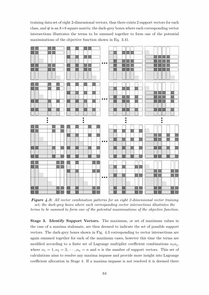
training data set of eight 2-dimensional vectors, thus there exists 2 support vectors for each
class, and ψ is an 8×8 square matrix; the dark-grey boxes where each corresponding vector
intersections illustrates the terms to be summed together to form one of the potential
maximisations of the objective function shown in Eq. 3.41.
Figure 4.3: All vector combination patterns for an eight 2-dimensional vector trainingset; the dark-grey boxes where each corresponding vector intersections illustrates the
terms to be summed to form one of the potential maximisations of the objective function.
Stage 3. Identify Support Vectors. The maximum, or set of maximum values in
the case of a maxima stalemate, are then deemed to indicate the set of possible support
vectors. The dark-grey boxes shown in Fig. 4.3 corresponding to vector intersections are
again summed together for each of the maximum cases, however this time the terms are
modified according to a finite set of Lagrange multiplier coefficient combinations αiαj ,
where α1 = 1, α2 = 2, · · · , αn = n and n is the number of support vectors. This set of
calculations aims to resolve any maxima impasse and provide more insight into Lagrange
coefficient allocation in Stage 4. If a maxima impasse is not resolved it is deemed there
64

exits more than one set of unique support vectors and therefore any arbitrary choice of
the between the stalemate-factions will sufficiently serve.
Stage 4. Assign Lagrange Multiplier Values αi to Identified Support Vec-
tors. Observing the results of Stage 3. one can deduce which vectors of the training
data receive non-zero Lagrangian coefficients α and the fraction of the cost-constant C
these values will take. Care must be taken to ensure that Lagrange multipliers values are
allocated in pairs, where αisv+ = αisv− , and the constraint shown in Eq. 3.39 holds true.
Supplemental Stage. Optimal SVM Function-Model Evaluation. Using the re-
cently acquired Lagrange multiplier and support vector pairs {xisv+ , αisv+} and {xisv− , αisv−},one can now evaluate the optimum SVM function-model shown in Fig. 3.41 on new non-
training data; a general architectural structure for this stage is presented in Section 4.3.
Where appropriate signed unitary multiplication operations are replaced with appropri-
ate sign-bit modifying digital-logic circuitry for both computational-performance enhance-
ment and resource conservation.
Each parallel calculation of Stage 1. is carried out in two steps. The sign of each yiyj
class-coefficient pair and the kernel function ψ(xi, xj) are evaluated for i, j = 1, 2, · · · , k,
where k denotes the last training vector. The class-coefficients yiyj are assigned a binary
value, where
ai =
{1 for −ve yi
0 for +ve yi, (4.5)
and the sign-bit Yij of the pair is found, where
Yij = ai ⊕ aj . (4.6)
Then the sign-bit of each kernel function evaluation is XORed with each corresponding Yij ,
thus effectively evaluating −yiyjψ(xi, xj) with minimal costly multiplication operations.
Figure 4.4 provides an illustration of the Stage 1. architecture.
ai =
{1 for −ve yi0 for +ve yi
Yij = ai ⊕ ajwhere
ψ(xi, xj)
Stage 1. Hardware Architecture
Training Data To Stage 2.
S′ψij
= Sψij ⊕ Yij
ψ
Figure 4.4: Stage 1. hardware architecture overview.
Stages 2, 3, and 4 are are shown as architectural overviews in Fig. 4.5, Fig. 4.6, and
65

Fig. 4.7 respectively. Currently these stages use simple straight-forward logic and sorting
techniques, thus no further exposition into the underlying architecture is provided.
∑−yiyjψ(xi, xj)Stage 2. Hardware Architecture
for all possiblecombinations of ntraining vectors
List of objective-sumcombinations &
responsible trainingvector indices
To Stage 3.ψ
Figure 4.5: Stage 2. hardware architecture overview.
Stage 3. Hardware Architecture∑−αiαjyiyjψ(xi, xj)
for all possiblecombinations of n
temporary values of α
Determine SupportVector Indices
Objective-sum List To Stage 4.
Determine Maximum/s
Max objective-sumswith responsible
training vector indices& temp α values
Figure 4.6: Stage 3. hardware architecture overview.
Stage 4. Hardware Architecture
Assign actual α valueas some fraction of Cto each +1 and -1 classsupport vector pair
Optimal SupportVector Indices & actualα values vector α
To Supplimental SVMEvaluation Stage
Support Vector Indices& temp α values
Figure 4.7: Stage 4. hardware architecture overview.
Where appropriate, the DSP pipeline architectures presented in Fig. 4.29, Fig. 4.30, Fig.
A.1, Fig. A.2, Fig. A.3, Fig. 4.31, and Fig. 4.32 can be used to construct the brute-force
non-iterative fixed-period SVM classification training subsystem architecture.
As a proof-of-concept and verification of successful SVM training the architecture was
modelled using MATLAB. By applying the trained SVM to test data-sets with the goal
of correctly classifying the data, the SVM training scheme was thus validated as a feasible
mechanism for SVM training. All parallel processes inherent in the design were modelled
in a sequential manner.
The design was tested using a simple 2-dimensional linearly-separable problem train-
66

ing data-set utilising the dot-product kernel, the no-kernel variation of the SVM. The
number of computations for Stage 1 to Stage 4 were estimated to be 765, 12960, 12960,
and 4 operations respectively. The derived Lagrangian coefficients and support vectors
were then applied to SVM function-model evaluation with a different linearly-separable
testing data-set. Both training and testing linearly-separable data-sets are shown in Fig.
4.8. The linearly-separable testing data-set was classified with 100% accuracy.
0
2
4
6
8
10
0 2 4 6 8 10
x2
x10
2
4
6
8
10
0 2 4 6 8 10
x2
x10
2
4
6
8
10
0 2 4 6 8 10
x2
x1
Figure 4.8: Simple linearly-separable problem datasets; +1 class and -1 class trainingdata are shown as circles and dots respectively, testing data is shown as crosses.
The design was also tested using a standard 2-dimensional XOR problem training data-set
utilising a polynomial kernel. The number of computations for Stage 1 to Stage 4 were
estimated to be 1224, 12960, 12960, and 4 operations respectively. The derived Lagrangian
coefficients and support vectors were then applied to SVM function-model evaluation with
a different XOR testing data-set. Both training and testing XOR data-sets are shown in
Fig. 4.9. The XOR testing dataset was classified with 100% accuracy.
−5
0
5
10
−10 −5 0 5 10
x2
x1
−5
0
5
10
−10 −5 0 5 10
x2
x1
−5
0
5
10
−10 −5 0 5 10
x2
x1
Figure 4.9: XOR problem datasets; +1 class and -1 class training data are shown ascircles and dots respectively, testing data is shown as crosses.
67

4.1.2 Combined Exterior Penalty and Barrier Function Optimisation
The combined exterior penalty function and interior penalty / barrier function optimisa-
tion technique, shown in Eq. 3.62, was developed for the SVM classification problem as
follows. The soft-margin support vector model is trained by optimising the Lagrangian
arg maxα
φ′(α) = arg maxα
k∑
i=1
αi −1
2
k∑
i=1
k∑
j=1
αiαjyiyjψ(xi, xj)
, (4.7)
subject to the constraints
k∑
i=1
αiyi = 0, (4.8)
αi ≥ 0, and (4.9)
C − αi ≥ 0, (4.10)
where i = 1, · · · , k and C is the cost constant.
Applying the extended interior approach the constrained optimisation problem shown in
Eq. 4.7 , Eq. 4.8, Eq. 4.9 and Eq. 4.10 is converted into an unconstrained minimisation
problem by constructing an energy function of the form
E(α, κ) = φ(α) + κ0h2(α) +
1
κ1B1(α) +
1
κ2B2(α), (4.11)
where
φ(α) = −k∑
i=1
αi +1
2
k∑
i=1
k∑
j=1
αiαjyiyjψ(xi, xj), (4.12)
h(α) =k∑
i=1
αiyi, (4.13)
where κ0 > 0, κ1 > 0, and κ2 > 0, and where B1(α) and B2(α) are the extended barrier
functions
B1(αj) =
1
αj, if αj ≥ ε,
2ε− αjε2
, if αj < ε, and
(4.14)
B2(αj) =
1
C − αj, if C − αj ≥ ε,
2ε− C + αjε2
, if C − αj < ε,
(4.15)
where ε is a small positive number which determines the transition from the exterior ex-
tended penalty to the interior penalty functions.
Applying standard gradient descent technique a system of differential equations is con-
68
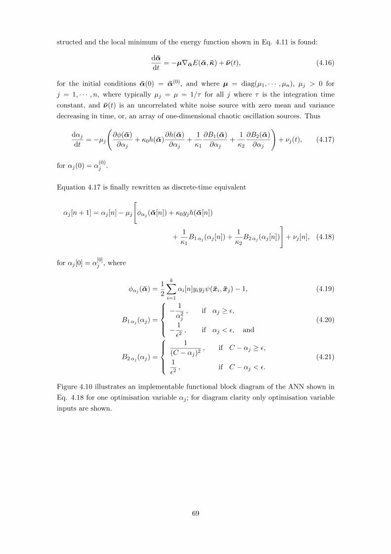
structed and the local minimum of the energy function shown in Eq. 4.11 is found:
dα
dt= −µ∇αE(α, κ) + ν(t), (4.16)
for the initial conditions α(0) = α(0), and where µ = diag(µ1, · · · , µn), µj > 0 for
j = 1, · · · , n, where typically µj = µ = 1/τ for all j where τ is the integration time
constant, and ν(t) is an uncorrelated white noise source with zero mean and variance
decreasing in time, or, an array of one-dimensional chaotic oscillation sources. Thus
dαjdt
= −µj(∂φ(α)
∂αj+ κ0h(α)
∂h(α)
∂αj+
1
κ1
∂B1(α)
∂αj+
1
κ2
∂B2(α)
∂αj
)+ νj(t), (4.17)
for αj(0) = α(0)j .
Equation 4.17 is finally rewritten as discrete-time equivalent
αj [n+ 1] = αj [n]− µj[φαj (α[n]) + κ0yjh(α[n])
+1
κ1B1αj (αj [n]) +
1
κ2B2αj (αj [n])
]+ νj [n], (4.18)
for αj [0] = α[0]j , where
φαj (α) =1
2
k∑
i=1
αi[n]yiyjψ(xi, xj)− 1, (4.19)
B1αj (αj) =
− 1
α2j
, if αj ≥ ε,
− 1
ε2, if αj < ε, and
(4.20)
B2αj (αj) =
1
(C − αj)2, if C − αj ≥ ε,
1
ε2, if C − αj < ε.
(4.21)
Figure 4.10 illustrates an implementable functional block diagram of the ANN shown in
Eq. 4.18 for one optimisation variable αj ; for diagram clarity only optimisation variable
inputs are shown.
69

κ1
φαj (α[n])
α1[n]αj [n]
αk[n]
yj
(k∑
i=1
αiyi
)
− 1
ε2
− 1
α2j
1
(C − αj)2
κ0
−µj
κ2
αj [n+ 1]
ε
ε
· · ·· · ·
C − αj
νj [n]
Figure 4.10: Functional block-diagram of the ANN-mapped combined exterior penaltyfunction and interior penalty / barrier function optimisation technique for SVM
classification as defined in Eq. 4.18.
The combined exterior penalty function and interior penalty / barrier function optimi-
sation technique, shown in Eq. 3.62, was developed for the SVM regression problem as
follows. The soft-margin support vector model for regression is trained by optimising the
Lagrangian
arg maxα•,α◦
φ′(α•, α◦) = arg maxα•,α◦
−1
2
k∑
i=1
k∑
j=1
(α•i − α◦i )(α•j − α◦j )ψ(xi, xj)
+k∑
i=1
yi(α•i − α◦i )− η
k∑
i=1
(α•i + α◦i )
), (4.22)
subject to the constraints
k∑
i=1
(α•i − α◦i ) = 0, (4.23)
α◦i ≥ 0, and (4.24)
C − α•i ≥ 0, (4.25)
where i = 1, · · · , k and C is the cost constant.
Applying the extended interior approach the constrained optimisation problem shown
70

in Eq. 4.22 , Eq. 4.23, Eq. 4.24 and Eq. 4.25 is converted into an unconstrained
minimisation problem by constructing an energy function of the form
E(α•, α◦, κ) = φ(α•, α◦) + κ0h2(α•, α◦) +
1
κ1B1(α•, α◦) +
1
κ2B2(α•, α◦), (4.26)
where
φ(α•, α◦) =1
2
k∑
i=1
k∑
j=1
(α•i−α◦i )(α•j−α◦j )ψ(xi, xj)−k∑
i=1
yi(α•i−α◦i )+η
k∑
i=1
(α•i +α◦i ), (4.27)
h(α•, α◦) =
k∑
i=1
(α•i − α◦i ), (4.28)
where κ0 > 0, κ1 > 0, and κ2 > 0, and where B1(α•, α◦) and B2(α•, α◦) are the extended
barrier functions
B1(α•j , α◦j ) =
1
α◦j, if α◦j ≥ ε,
2ε− α◦jε2
, if α◦j < ε, and
(4.29)
B2(α•j , α◦j ) =
1
C − α•j, if C − α•j ≥ ε,
2ε− C + α•jε2
, if C − α•j < ε,
(4.30)
where ε is a small positive number which determines the transition from the exterior ex-
tended penalty to the interior penalty functions.
Applying standard gradient descent technique a system of differential equations is con-
structed and the local minimum of the energy function shown in Eq. 4.11 is found:
dα•
dt= −µ∇α•E(α•, α◦, κ) + να•(t), (4.31)
dα◦
dt= −ρ∇α◦E(α•, α◦, κ) + να◦(t), (4.32)
for the initial conditions α(0) = α(0) and where µ = diag(µ1, · · · , µn) and ρ = diag(ρ1, · · · , ρn),
µj > 0 and ρj > 0 for j = 1, · · · , n, where typically µj = µ = ρj = ρ = 1/τ for all j where
τ is the integration time constant, and να•(t) and να◦(t) are uncorrelated white noise
sources with zero mean and variance decreasing in time, or, are arrays of one-dimensional
chaotic oscillation sources. Thus
dα•jdt
= −µj(∂φ(α•, α◦)
∂α•j+ κ0h(α•, α◦)
∂h(α•, α◦)∂α•j
+1
κ1
∂B1(α•, α◦)∂α•j
+1
κ2
∂B2(α•, α◦)∂α•j
)+ να•
j(t), (4.33)
71

and
dα◦jdt
= −ρj(∂φ(α•, α◦)
∂α◦j+ κ0h(α•, α◦)
∂h(α•, α◦)∂α◦j
+1
κ1
∂B1(α•, α◦)∂α◦j
+1
κ2
∂B2(α•, α◦)∂α◦j
)+ να◦
j(t), (4.34)
for αj(0) = α(0)j .
Equation 4.33 and 4.34 are finally rewritten as discrete-time equivalents
α•j [n+ 1] = α•j [n]− µj[φα•
j(α•[n], α◦[n]) + κ0h(α•[n], α◦[n])
+1
κ1B1α•
j(α•j [n], α◦j [n]) +
1
κ2B2α•
j(α•j [n], α◦j [n])
]+ να•
j[n], (4.35)
and
α◦j [n+ 1] = α◦j [n]− ρj[φα◦
j(α•[n], α◦[n])− κ0h(α•[n], α◦[n])
+1
κ1B1α◦
j(α•j [n], α◦j [n]) +
1
κ2B2α◦
j(α•j [n], α◦j [n])
]+ να◦
j[n], (4.36)
for αj [0] = α[0]j , where
φα•j(α•[n], α◦[n]) =
k∑
i=1
(α•i − α◦i )ψ(xi, xj)− yj + η, and (4.37)
φα◦j(α•[n], α◦[n]) =
k∑
i=1
(α◦i − α•i )ψ(xi, xj) + yj + η, (4.38)
where m = 1, · · · , k, and
B1α•j(α•j [n], α◦j [n]) = 0, (4.39)
B2α•j(α•j [n], α◦j [n]) =
1
(C − α•j )2, if C − α•j ≥ ε,
1
ε2, if C − α•j < ε,
(4.40)
B1α◦j(α•j [n], α◦j [n]) =
− 1
(α◦j )2, if α◦j ≥ ε,
− 1
ε2, if α◦j < ε, and
(4.41)
B2α◦j(α•j [n], α◦j [n]) = 0. (4.42)
Figure 4.11 and Fig. 4.12 illustrate implementable functional block diagrams of the ANNs
72

shown in Eq. 4.35 and Eq. 4.36 for one optimisation variable α•j and α◦j respectively; for
diagram clarity only optimisation variable inputs are shown.
φα•j(α•, α◦)
k∑
i=1
(α•i − α◦
i )
1
ε2
1
(C − α•j )
2
κ0
−µj
1
κ2
α•j [n+ 1]
εC − α•
j
να•j[n]
α◦1[n]α◦j [n]α◦k[n]
· · ·· · ·
α•1[n]α•j [n]α•k[n]
· · ·· · ·
Figure 4.11: Functional block-diagram of the ANN-mapped combined exterior penaltyfunction and interior penalty / barrier function optimisation technique for SVM
regression as defined in Eq. 4.35.
1
κ1
φα◦j(α•, α◦)
k∑
i=1
(α•i − α◦
i )
− 1
ε2
− 1
(α◦j )
2
−κ0
−ρj
α◦j [n+ 1]
ε
να◦j[n]
α◦1[n]α◦j [n]α◦k[n]
· · ·· · ·
α•1[n]α•j [n]α•k[n]
· · ·· · ·
Figure 4.12: Functional block-diagram of the ANN-mapped combined exterior penaltyfunction and interior penalty / barrier function optimisation technique for SVM
regression as defined in Eq. 4.36.
73

4.1.3 Augmented Lagrange Multiplier Optimisation
The Augmented Lagrange Multiplier ANN optimisation technique, shown in Eq. 3.72 and
Eq. 3.73, was developed for the SVM classification problem as follows. The soft-margin
support vector model is trained by optimising the Lagrangian
arg maxα
φ′(α) = arg maxα
k∑
i=1
αi −1
2
k∑
i=1
k∑
j=1
αiαjyiyjψ(xi, xj)
, (4.43)
subject to the constraints
k∑
i=1
αiyi = 0, (4.44)
αi ≥ 0, and (4.45)
C − αi ≥ 0, (4.46)
where i = 1, · · · , k and C is the cost constant.
The augmented Lagrangian is constructed from the constrained optimisation problem
shown in Eq. 4.43, Eq. 4.44, Eq. 4.45, and Eq. 4.45 and takes the form
L(α, λ, κ) = φ(α) + λ0h0(α) +κ1
2h2
0(α)
+k∑
j=1
(λjgj(αj) +
κ2
2g2j (αj)
)+
k∑
j=1
(λk+jgk+j(αj) +
κ3
2g2k+j(αj)
)(4.47)
where
φ(α) = −k∑
i=1
αi +1
2
k∑
i=1
k∑
j=1
αiαjyiyjψ(xi, xj), (4.48)
h0(α) =
k∑
i=1
αiyi, (4.49)
and
gj(αj) =
αj , if αj < −λjκj,
−λjκj, if αj ≥ −
λjκj,
(4.50)
gk+j(αj) =
C − αj , if C − αj < −λk+j
κk+j,
−λk+j
κk+j, if C − αj ≥ −
λk+j
κk+j,
(4.51)
74

where j = 1, · · · , n and κi ≥ 0 is the penalty parameter. The minimisation of the
augmented Lagrangian can be converted into a system of differential equations
dα
dt= −µ∇αL(α, λ, κ) + να(t), (4.52)
dλ
dt= ρ∇λL(α, λ, κ) + νλ(t), (4.53)
where µ = diag(µ1, · · · , µn) and ρ = diag(ρ1, · · · , ρm) are positive scalar variables, typ-
ically chosen as µi > 0 and ρi > 0, and with the initial conditions α(0) = α(0) and
λ(0) = λ(0)
. This can be written in scalar form
dαjdt
= −µj(∂φ(α)
∂αj+ λ0
∂h0(α)
∂αj+κ0
2h0(α)
∂h0(α)
∂αj
+ λj∂gj(αj)
∂αj+κj2gj(αj)
∂gj(αj)
∂αj+
λk+j∂gk+j(αj)
∂αj+κk+j
2gk+j(αj)
∂gk+j(αj)
∂αj
)+ ναj (t), (4.54)
and
dλ0
dt= ρ0
(h0(α)
)+ νλ0(t), (4.55)
dλjdt
=
ρj(αj)
+ νλj (t), if αj < −λjκj,
νλj (t), if αj ≥ −λjκj,
(4.56)
dλk+j
dt=
ρk+j
(C − αj
)+ νλk+j (t), if C − αj < −
λk+j
κk+j,
νλk+j (t), if C − αj ≥ −λk+j
κk+j,
(4.57)
Equation 4.54, Eq. 4.55, Eq. 4.56, and Eq. 4.57 are finally rewritten as discrete-time
equivalents
αj [n+ 1] = αj [n]− µj[φαj (α) + h0αj (α)
(λ0[n] +
κ0
2h0(α)
)
+ gjαj (αj)
(λj [n] +
κj2gj(αj)
)
+ gk+jαj (αj)
(λk+j [n] +
κk+j
2gk+j(αj)
)]+ ναj [n], (4.58)
75

and
λ0[n+ 1] = λ0[n] + ρ0
[h0(α)
]+ νλ0 [n], (4.59)
λj [n+ 1] =
λj [n] + ρj
[αj [n]
]+ νλj [n], if αj [n] < −λj [n]
κj,
λj [n] + νλj [n], if αj [n] ≥ −λj [n]
κj,
(4.60)
λk+j [n+ 1] =
λk+j [n] + ρk+j
[C − αj [n]
]+ νλk+j [n], if C − αj [n] < −λk+j [n]
κk+j,
λk+j [n] + νλk+j [n], if C − αj [n] ≥ −λk+j [n]
κk+j,
(4.61)
where
φαj (α) =1
2
k∑
i=1
αi[n]yiyjψ(xi, xj)− 1, (4.62)
h0(α) =k∑
i=1
αi[n]yi, (4.63)
h0αj (α) = yj , (4.64)
gj(αj) =
αj [n], if αj [n] < −λj [n]
κj,
−λj [n]
κj, if αj [n] ≥ −λj [n]
κj,
(4.65)
gjαj (αj) =
1, if αj [n] < −λj [n]
κj,
0, if αj [n] ≥ −λj [n]
κj,
(4.66)
gk+j(αj) =
C − αj [n], if C − αj [n] < −λk+j [n]
κk+j,
−λk+j [n]
κk+j, if C − αj [n] ≥ −λk+j [n]
κk+j,
(4.67)
gk+jαj (αj) =
−1, if C − αj [n] < −λk+j [n]
κk+j,
0, if C − αj [n] ≥ −λk+j [n]
κk+j,
(4.68)
Figure 4.13 and Fig. 4.14 illustrate implementable functional block diagrams of the ANN
shown in Eq. 4.58, Eq. 4.59, Eq. 4.60 and Eq. 4.61 for the optimisation variables
αj , λ0, λj and λk+j ; for diagram clarity only optimisation variable inputs are shown.
76

α1[n]αj [n]
αk[n]
k∑
i=1
αi[n]yi
αj [n+ 1]
· · ·· · · ναj [n]
yj
1
2
k∑
i=1
αi[n]yiyjψ(xi, xj)− 1
λ0[n]
λj [n]
λk+j [n]
C − αj [n]
− 1
κk+j
− 1
κj
κ0
2
−µj
10
κj
2
−10
κj
2
Figure 4.13: Functional block-diagram of the ANN-mapped augmented LagrangeMultiplier optimisation technique as defined in Eq. 4.58.
α1[n]αj [n]
αk[n]
k∑
i=1
αi[n]yi
λ0[n+ 1]· · ·· · ·
νλ0[n]
λ0[n]
λj [n]
λk+j [n]
C − αj [n]
− 1
κk+j
− 1
κj
ρ0
ρj
0
0
ρk+j
λj [n+ 1]
νλj [n]
νλk+j[n]
λk+j [n+ 1]
Figure 4.14: Functional block-diagram of the ANN-mapped augmented LagrangeMultiplier optimisation technique as defined in Eq. 4.59, Eq. 4.60, and Eq. 4.61.
77

The Augmented Lagrange Multiplier ANN optimisation technique, shown in Eq. 3.72
and Eq. 3.73, was developed for the SVM regression problem as follows. The soft-margin
support vector model for regression is trained by optimising the Lagrangian
arg maxα•,α◦
φ′(α•, α◦) = arg maxα•,α◦
−1
2
k∑
i=1
k∑
j=1
(α•i − α◦i )(α•j − α◦j )ψ(xi, xj)
+k∑
i=1
yi(α•i − α◦i )− η
k∑
i=1
(α•i + α◦i )
), (4.69)
subject to the constraints
k∑
i=1
(α•i − α◦i ) = 0, (4.70)
α◦i ≥ 0, and (4.71)
C − α•i ≥ 0, (4.72)
where i = 1, · · · , k and C is the cost constant.
The augmented Lagrangian is constructed from the constrained optimisation problem
shown in Eq. 4.69, Eq. 4.70, Eq. 4.71, and Eq. 4.71 and takes the form
L(α•, α◦, λ, κ) = φ(α•, α◦) + λ0h0(α•, α◦) +κ1
2h2
0(α•, α◦)
+
k∑
j=1
(λjgj(α
•j , α◦j ) +
κ2
2g2j (α•j , α◦j )
)+
k∑
j=1
(λk+jgk+j(α
•j , α◦j ) +
κ3
2g2k+j(α
•j , α◦j )
)
(4.73)
where
φ(α•, α◦) =1
2
k∑
i=1
k∑
j=1
(α•i − α◦i )(α•j − α◦j )ψ(xi, xj)
−k∑
i=1
yi(α•i − α◦i ) + η
k∑
i=1
(α•i + α◦i ), (4.74)
h0(α•, α◦) =k∑
i=1
(α•i − α◦i ), (4.75)
78

and
gj(α•j , α◦j ) =
α◦j , if α◦j < −λjκj,
−λjκj, if α◦j ≥ −
λjκj,
(4.76)
gk+j(α•j , α◦j ) =
C − α•j , if C − α•j < −λk+j
κk+j,
−λk+j
κk+j, if C − α•j ≥ −
λk+j
κk+j,
(4.77)
where j = 1, · · · , n and κi ≥ 0 is the penalty parameter. The minimisation of the
augmented Lagrangian can be converted into a system of differential equations
dα•
dt= −µα•∇α•L(α•, α◦, λ, κ) + να•(t), (4.78)
dα◦
dt= −µα◦∇α◦L(α◦, α◦, λ, κ) + να◦(t), (4.79)
dλ
dt= ρ∇λL(α•, α◦, λ, κ) + νλ(t), (4.80)
where µ = diag(µ1, · · · , µn) and ρ = diag(ρ1, · · · , ρm) are positive scalar variables, typ-
ically chosen as µi > 0 and ρi > 0, and with the initial conditions α(0) = α(0) and
λ(0) = λ(0)
. This can be written in scalar form
dα•jdt
= −µα•j
(∂φ(α•, α◦)
∂α•j+ λ0
∂h0(α•, α◦)
∂α•j+κ0
2h0(α•, α◦)
∂h0(α•, α◦)
∂α•j
+ λj∂gj(α
•j , α◦j )
∂α•j+κj2gj(α
•j , α◦j )∂gj(α
•j , α◦j )
∂α•j+
λk+j
∂gk+j(α•j , α◦j )
∂α•j+κk+j
2gk+j(α
•j , α◦j )∂gk+j(α
•j , α◦j )
∂α•j
)+ να•
j(t), (4.81)
dα◦jdt
= −µα◦j
(∂φ(α•, α◦)
∂α◦j+ λ0
∂h0(α•, α◦)
∂α◦j+κ0
2h0(α•, α◦)
∂h0(α•, α◦)
∂α◦j
+ λj∂gj(α
•j , α◦j )
∂α◦j+κj2gj(α
•j , α◦j )∂gj(α
•j , α◦j )
∂α◦j+
λk+j
∂gk+j(α•j , α◦j )
∂α◦j+κk+j
2gk+j(α
•j , α◦j )∂gk+j(α
•j , α◦j )
∂α◦j
)+ να◦
j(t), (4.82)
79

and
dλ0
dt= ρ0
(h0(α•, α◦)
)+ νλ0(t), (4.83)
dλjdt
=
ρj(α◦j)
+ νλj (t), if α◦j < −λjκj,
νλj (t), if α◦j ≥ −λjκj,
(4.84)
dλk+j
dt=
ρk+j
(C − α•j
)+ νλk+j (t), if C − α•j < −
λk+j
κk+j,
νλk+j (t), if C − α•j ≥ −λk+j
κk+j,
(4.85)
Equation 4.81, Eq. 4.82 Eq. 4.83, Eq. 4.84, and Eq. 4.85 are finally rewritten as
discrete-time equivalents
α•j [n+ 1] = α•j [n]− µα•j
[φα•
j(α•, α◦) + h0α•
j(α•, α◦)
(λ0[n] +
κ0
2h0(α•, α◦)
)
+ gjα•j(α•j , α
◦j )
(λj [n] +
κj2gj(α
•j , α◦j )
)
+ gk+jα•j(α•j , α
◦j )
(λk+j [n] +
κk+j
2gk+j(α
•j , α◦j )
)]+ να•
j[n], (4.86)
α◦j [n+ 1] = α◦j [n]− µα◦j
[φα◦
j(α•, α◦) + h0α◦
j(α•, α◦)
(λ0[n] +
κ0
2h0(α•, α◦)
)
+ gjα◦j(α•j , α
◦j )
(λj [n] +
κj2gj(α
•j , α◦j )
)
+ gk+jα◦j(α•j , α
◦j )
(λk+j [n] +
κk+j
2gk+j(α
•j , α◦j )
)]+ να◦
j[n], (4.87)
and
λ0[n+ 1] = λ0[n] + ρ0
[h0(α•, α◦)
]+ νλ0 [n], (4.88)
λj [n+ 1] =
λj [n] + ρj
[α◦j [n]
]+ νλj [n], if α◦j [n] < −λj [n]
κj,
λj [n] + νλj [n], if α◦j [n] ≥ −λj [n]
κj,
(4.89)
λk+j [n+ 1] =
λk+j [n] + ρk+j
[C − α•j [n]
]+ νλk+j [n], if C − α•j [n] < −λk+j [n]
κk+j,
λk+j [n] + νλk+j [n], if C − α•j [n] ≥ −λk+j [n]
κk+j,
(4.90)
80

where
φα•j(α•[n], α◦[n]) =
k∑
i=1
(α•i − α◦i )ψ(xi, xj)− yj + η, and (4.91)
φα◦j(α•[n], α◦[n]) =
k∑
i=1
(α◦i − α•i )ψ(xi, xj) + yj + η, (4.92)
h0(α•, α◦) =k∑
i=1
(α•i − α◦i ), (4.93)
h0α•j(α•, α◦) = 1, (4.94)
h0α◦j(α•, α◦) = −1, (4.95)
gj(α•j , α◦j ) =
αj [n]◦, if αj [n]◦ < −λj [n]
κj,
−λj [n]
κj, if αj [n]◦ ≥ −λj [n]
κj,
(4.96)
gjα•j(α•j , α
◦j ) =
0, if αj [n]◦ < −λj [n]
κj,
0, if αj [n]◦ ≥ −λj [n]
κj,
(4.97)
gjα◦j(α•j , α
◦j ) =
1, if αj [n]◦ < −λj [n]
κj,
0, if αj [n]◦ ≥ −λj [n]
κj,
(4.98)
gk+j(α•j , α◦j ) =
C − αj [n]•, if C − αj [n]• < −λk+j [n]
κk+j,
−λk+j [n]
κk+j, if C − αj [n]• ≥ −λk+j [n]
κk+j,
(4.99)
gk+jα•j(α•j , α
◦j ) =
−1, if C − αj [n]• < −λk+j [n]
κk+j,
0, if C − αj [n]• ≥ −λk+j [n]
κk+j,
(4.100)
gk+jα◦j(α•j , α
◦j ) =
0, if C − αj [n]• < −λk+j [n]
κk+j,
0, if C − αj [n]• ≥ −λk+j [n]
κk+j,
(4.101)
(4.102)
Figure 4.15, Fig. 4.16 and Fig. 4.17 illustrate implementable functional block diagrams
of the ANN shown in Eq. 4.86, Eq. 4.87, Eq. 4.88, Eq. 4.89 and Eq. 4.90 for the opti-
misation variables α•j , α◦j , λ0, λj and λk+j ; for diagram clarity only optimisation variable
inputs are shown.
81

k∑
i=1
(α•i − α◦
i )
α•j [n+ 1]
να•j[n]
1
k∑
i=1
(α•i −α◦
i )ψ(xi, xm)−yj+η
λ0[n]
λk+j [n]
C − α•j [n]
− 1
κk+j
κ0
2
−µα•j
−10
κj
2
α◦1[n]α◦j [n]α◦k[n]
· · ·· · ·
α•1[n]α•j [n]α•k[n]
· · ·· · ·
Figure 4.15: Functional block-diagram of the ANN-mapped augmented LagrangeMultiplier optimisation technique as defined in Eq. 4.86.
k∑
i=1
(α•i − α◦
i )
α◦j [n+ 1]
να◦j[n]
−1
k∑
i=1
(α◦i −α•
i )ψ(xi, xm)+yj+η
λ0[n]
λj [n]
− 1
κj
κ0
2
−µα◦j
10
κj
2
α◦1[n]α◦j [n]α◦k[n]
· · ·· · ·
α•1[n]α•j [n]α•k[n]
· · ·· · ·
Figure 4.16: Functional block-diagram of the ANN-mapped augmented LagrangeMultiplier optimisation technique as defined in Eq. 4.87.
82
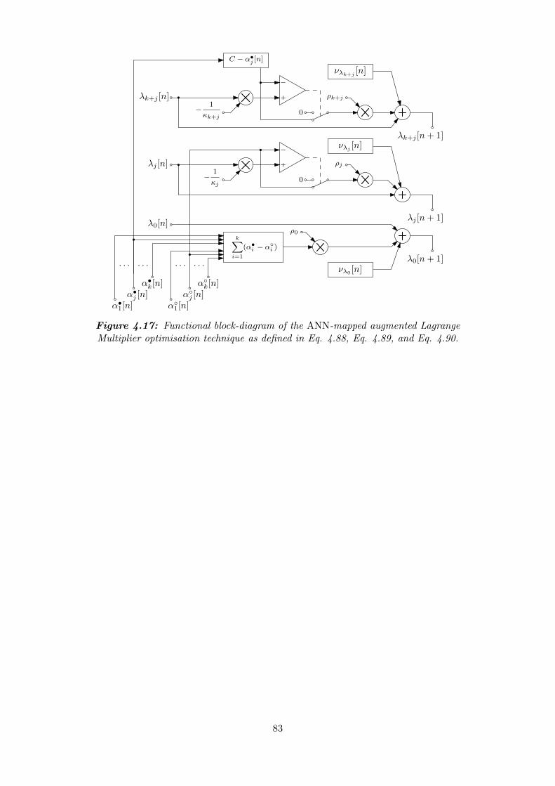
k∑
i=1
(α•i − α◦
i )
λ0[n+ 1]νλ0
[n]
λ0[n]
λj [n]
λk+j [n]
C − α•j [n]
− 1
κk+j
− 1
κj
ρ0
ρj
0
0
ρk+j
λj [n+ 1]
νλj [n]
νλk+j[n]
λk+j [n+ 1]
α◦1[n]α◦j [n]α◦k[n]
· · ·· · ·
α•1[n]α•j [n]α•k[n]
· · ·· · ·
Figure 4.17: Functional block-diagram of the ANN-mapped augmented LagrangeMultiplier optimisation technique as defined in Eq. 4.88, Eq. 4.89, and Eq. 4.90.
83

4.2 SVM Test-Rig System Hardware Architecture
This section provides details of the SVM test-rig system architecture design and im-
plementation. This includes design methodology considerations, physical FPGA develop-
ment platform considerations, FPGA development and supporting software considerations
and procurement, and, system-level and modular low-level FPGA hardware architecture
design and implementation details. As design methodology and hardware development
practicalities are shared across both the SVM test-rig system hardware and the SVM DSP
pipeline hardware all cursory DSP pipeline considerations are addressed in this subsection.
However all specific technical design details are addressed in Section 4.3.
4.2.1 FPGA Platform and Implementation Considerations
The primary motivation for this research, and thus principal design performance param-
eter for the SVM system, is achieving real-time SVM performance - the computational
latency or execution time is equal or is less than equal to the period between each succes-
sive input data sample. Therefore, the goal of this project is succinctly summarised by
considering the following two research questions. What is the minimum latency that can
be achieved by an FPGA-based SVM implementation over some subset of design varia-
tions? What is the minimum period between each successive input data sample applied to
an FPGA-based SVM implementation to maintain real-time operation?
The core consideration and thus fundamental justification for implementing the SVM
system as FPGA hardware is the goal of achieving real-time performance. Implemented
via traditional software-based mechanisms, the maximum concurrently executed opera-
tions is limited by the number of cores a Central Processing Unit (CPU) is composed of,
or, the number of threads each CPU core can concurrently execute. An FPGA hardware
implementation by comparison can concurrently execute operations several orders of mag-
nitude greater than a traditional CPU architecture. As the SVM is such a highly mathe-
matical operation-rich paradigm it is thus well suited to a parallelised systolic pipelined
implementation. Utilising a multi-threaded CPU based implementation such a system
is still limited to some small finite-thread set of sequentially executed operations. An
FPGA-based implementation can be designed such that massively-parallel and concur-
rent systolic pipelined operations are executed in large volume each system clock cycle.
Though an General-purpose Computing on Graphics Processing Units (GPGPU) based
implementation could serve as a possible design solution, it would still require a PC-system
backbone for operation. This is an undesirable solution and introduces unnecessary con-
straints and will pose infrastructural problems for field-based instrumentation adaptation.
An FPGA implementation allows for massively-parallel and systolic mathematical op-
eration execution, and, concurrent pipelined execution of these operations. The decision
to implement the system using FPGA technologies over other technologies was a matter
84
of sequential execution vs. systolic, parallel, and pipelined-processing-element execution,
and the ease of such an implementation concerning both physical (standalone FPGA
vs. GPGPU implementation and required supporting-infrastructure) and abstract imple-
mentation mechanisms (VHDL vs. software and API frameworks, such as CUDA and
OpenCL).
Engineering parameters and metrics, such as gate-count, functional-block and DSP-block
usage, and power consumption, are not presented as design constraints as they were sec-
ondary metrics to be measured and explored with design variation as part of this research
work. This work was a pure research and development exercise as opposed to the develop-
ment of an industrial or commercial product based on existing research and technological
and financial constraints; these metrics were thus regarded as unknown during the design
and development process. Minimising these metrics is, however, valid future work and
will certainly feature amongst future product development requirements.
4.2.2 Design Methodology Considerations
The system was designed and implemented using both concurrent development and a
combination of top-down and bottom-up modular design methodologies. The combina-
tion and application of these methodologies was appropriate for this research and de-
velopment endeavour. By designing each modular subsystem implementation in parallel
with an evolving system-wide design target and the greater development effort, inevitable
design adjustments were easily made and ensured a final set of designs and implementa-
tions that were fit for final application purpose, and, provided appropriate information
and metrics that contribute toward the goals of this research.
For example low-level modular FPGA processes such as multiplication and addition op-
erations were implemented by various methods, were subsequently tested, and finally
appropriate verification and functional testing outcomes were compared and contrasted.
These low-level development tasks were completed concurrently with the design and de-
velopment of the higher-level SVM system architectures. Once unexpected transient
behaviour or erroneous operation were resolved or mitigated the verified subsystems in
question were integrated, with minimal re-engineering or systems reintegration effort, to
form higher-level subsystems that were again tested and verified accordingly. The higher-
level modular subsystems were then again integrated until the ultimate-system design
was achieved. At each subsystem integration stage any testing problems or hardware
bugs that became apparent were easily identified and attributed to the offending subsys-
tem implementation and appropriate modifications or mitigations were made. Through
this design and development process subsystems were integrated as required and realised
with minimal additional debugging and testing requirements.
A benefit observed through the application of concurrent top-down and bottom-up mod-
ular design and development methodologies in this work was the division of labour and
85

its consequent advantages. By concurrently maintaining several active research and de-
velopment tasks, when any one of these pursuits stagnated or become obstructed for
any reason, overall system development did not stop and thus research and development
productivity was sustained. Also, the introduction of alternative techniques or methods
acquired through new literature or development serendipity was quickly assimilated and
integrated and into system designs by the introduction of either another modular compo-
nent or trivial modification to an existing component.
All designs are, however, presented in a modular top-down manner in this thesis. This
modular top-down presentation allows for a thorough design prescription while remain-
ing both succinct and comprehensible to the reader and the author alike. A modular
top-down presentation such as this also lends itself well to the comprehension of each
modular VHDL implementation. Conversely the reproduction of complicated and un-
wieldy circuit-diagram designs, as observed in the bygone-era of discrete-logic design, is
redundant due to the nature and application of the VHDL language and synthesis process.
Such a pursuit requires the lengthy and error-prone partitioning of subsystems followed by
their conversion back to high-level hardware descriptions compatible with modern FPGA
development and synthesis tools. Such a divergence from modern digital-system design
practises are universally deemed an inappropriate and inefficient endeavour, thus have no
place in modern digital-system design [67] and do not feature in such a form in this thesis.
4.2.3 FPGA Development Platform Considerations
The selection of FPGA vendor, and thus target FPGA device, was made early in the
work’s design and development phases. The following exposition provides insight into
nomination of Altera FPGA devices over their market competitor Xilinx FPGA devices.
Factors that influenced these decisions included available development tools, access to
FPGA development boards, and finally FPGA target device technology and technical
specifications.
The author was familiar with both Xilinx and Altera development tools, software suites,
and FPGA technology, and had developed digital logic targeting both vendor’s respective
FPGA technologies. Informed by this professional experience the author found Altera’s
development suite, Quartus II (now known as Quartus Prime [87]), superior to Xilinx’s
development suite ISE (now superseded by Xilinx Vivado Design Suite [88]) in ease of use,
system compilation and synthesis error reporting, and system instantiation and FPGA
programming.
Stemming from convenience and pragmatism the choice of FPGA vendor was also in-
fluenced by the development tools available to the author from the work’s outset. The
author was in possession of two Altera FPGA development boards; the Terasic DE1
development board utilising an Altera Cyclone II FPGA, and, the Terasic DE0-Nano
development board utilising an Altera Cyclone IV FPGA. From technology-generation,
86

hardware specification, and feature-set perspectives - including integrated USB JTAG
programming and debugging features - the Altera-based devices outclassed the Xilinx
Sparton-3 development boards available in the Department of Electrical and Electronic
Engineering at the University of Nottingham. Thus initial design and development efforts
began utilising the Terasic DE1 and DE0-Nano development boards. The Terasic DE1
and DE0-Nano development boards are shown in Fig. 4.18.
(a) (b)
Figure 4.18: Terasic Altera FPGA development boards; (a) the DE1 Cyclone IIdevelopment board, and (b) the DE0-Nano Cyclone IV development board.
Research funding was awarded in the form of a PRGS grant from the Government of
Malaysia. The grant’s focus was the development of a prototype real-time oil and gas
pipeline defect and failure detection system utilising the real-time SVM hardware archi-
tecture developed through this body of work. With this funding an Altera Stratix V DSP
development board was acquired. Figure 4.19 shows the Altera Stratix V DSP develop-
ment board that succeeded the Terasic DE1 and DE0-Nano development boards and was
used for all further research and development completed as part of this body of work.
Figure 4.19: Altera Stratix V DSP development Board.
As discussed in Subsection 4.2.1, the primary research goal of this work was to achieve
87

real-time performance; all other metrics and parameters were initially unknown. These
parameters were be investigated and explored in design variations. Also as discussed Sub-
section 4.2.1, the architecture was designed with the exploitation of massively parallel,
systolic, and pipelined processing-element potential of FPGA-based DSP implementa-
tions.
The Stratix V FPGA family was at the time of the Altera Stratix V DSP develop-
ment board acquisition the-top-of-the line and state-of-the-art Altera FPGA offering; the
potential for utilising the technology’s maximum specifications served the goal of this
research project - to explore and implement a real-time SVM system. Thus the platform
also served to provided a benchmark of measurable electrical and DSP-related parame-
ters across several design variations. For example the requirement for embedded DSP and
mathematical functional-block hardware far exceeds the need for raw implementable logic
available on the chosen target device - a requirement the Altera Stratix V GS 5SGSMD5
device found on the Altera Stratix V DSP development board met.
Finally for future extensions of this work - whether commercial, industrial, or research
based application - the Altera Stratix V device family serves as a good benchmark and
guaranteed platform, in terms of device life-span and commercial availability, to improve
upon system designs and thus improve derived and measured parameters and metrics
gained through the scientific application of this body of work.
4.2.4 Ancillary Software Tools
In addition to Altera Quartus II / Quartus Prime other ancillary software was employed
and utilised throughout the course of this research and development process. VHDL
debugging and simulation was conducted using Mentor Graphic’s ModelSim-Altera Edi-
tion simulation tool [89]. Algorithm and functional signal processing prototyping was
conducted using MathWork’s MATLAB [90] and the open-source equivalent GNU Oc-
tave [91]. Chaotic and non-linear time-series analysis was conducted using TISEAN:
Nonlinear Time Series Analysis tools [92]. All c software and software models were com-
piled with the gcc [93] toolchain and run on Arch Linux [94] systems. All source code was
managed using the Distributed Version Control System (DVCS) git [95] and all reposi-
tories were hosted privately on Atlassian Bitbucket [96] DVCS hosting service.
This thesis was written using LATEX [97]. All original plots found in this thesis were
generated with GNUPlot [98] and all original figures were created using the vector draw-
ing tool ipe [99].
4.2.5 System Design Considerations
Rajkumar’s proposed SVM system model is shown from a data-flow perspective in Fig.
4.20. The function blocks shown in grey, SVM Training and SVM Model Evaluation,
were the primary concern of this work’s research, design, and development efforts. This
88

included the implementation of a generalised FPGA hardware test-rig platform that can
be used to validate and test developed SVM hardware modules in both real-time and in
batch-processing mode. It was also required that the hardware platform be implemented
in a modular and extensible manner to allow for future research-driven extensions and
development with minimal VHDL refactoring requirements by undergraduate students
and research engineers with minimal correspondence with the original author.
SVM Training
Classification Model
Regression Model
SVM Model Evaluation
Classification Model
Regression Model
DataAcquisition
SignalProcessing
Input Signals Type ofDefect
DefectPrediction
& Timeto Failure
k-meansClustering /
kPCA
Figure 4.20: Simplified data-flow model of Rajkumar’s original work.
The hardware test-rig platform design and implementation conforms to the same data-flow
model as Rajkumar’s proposed system shown in Fig. 4.20.
4.2.6 SVM Test-Rig Design and Implementation
Figure 4.21 provides a system-level block-diagram of the FPGA hardware SVM test-
rig system and supplementary PC Terminal implementation and testing infrastructure
systems that were developed and employed as part of this body of work. The test-
rig hardware system has allowed for the thorough testing and rigorous application of
each developed SVM DSP pipeline. The SVM DSP pipeline subsystem architectures are
elaborated upon in Section 4.3.
FPGA HardwarePC TerminalTesting &Validation
DSP PipelineModels
MemoryManagement
SupplementarySoftware
SVMTraining
DataAnalysis
DataCache
SerialInterface
SPIInterface
ADC InputArray
SerialComms
Test-RigControl
DSPPipelines
Figure 4.21: Top-level block-diagram of the FPGA hardware test-rig system andsupplementary software subsystems.
The system shown in Fig. 4.21 has been implemented utilising pipelined computation
and data flow structures wherever possible and appropriate to maximise the test-rig sys-
tem’s overall data throughput capability and performance on the Altera Stratix V FPGA
hardware platform.
89

Figure. 4.22 provides a low-level hardware architectural overview of the developed SVM
test-rig system. The SVM test-rig system design incorporates a shared data bus with
individually mapped data bus lines to each subsystem module The shared data bus is
managed by a simple bus arbitration subsystem. Each test-rig subsystem is controlled by
the test-rig’s command and control subsystem. The test-rig system utilises three sepa-
rate and distinct uart cores - one uart is dedicated to system control and the other two
uart cores, db0 and db1, are available for low-level hardware debugging and reporting
apparatus. An input data cache in cache is utilised to store SVM training and function
evaluation parameters and batch processing data. An output data cache out cache is
utilised to store processed output data. The DSP pipeline module contains one of the
many SVM DSP pipelines developed as part of this work; the SVM DSP pipeline ar-
chitectures are discussed in Section 4.3. Finally the test-bench system design includes a
32-channel SPI array core to receive sampled real-world process data via an externally
connected 32-channel ADC hardware array.
FPGA: t0 svm
db0 DebugSerial Interface
db1 DebugSerial Interface
Input SignalArray
32 × 18-BitADC Channels
adc0
adc31
Control LogicSPI Array
Core
Shared Data Bus
3 × uart
Serial Cores
DSP PipelinesBus Arbitration Cache
PC Terminal
uart MainSerial Interface
Figure 4.22: Test-rig hardware system architectural overview.
The Altera Quartus Prime development suite was used to perform all circuit compilation,
optimisation, synthesis, and Altera Stratix V GS 5SGSMD5 FPGA device fitting and
subsequent programming as per the full set of developed VHDL code listings generated
through this work’s design and development efforts. The hierarchical VHDL module
dependency tree shown in Fig. 4.23 provides an overview of the system’s VHDL code-
base and its modular structure.
90

.vhd
svm
t0
uart
.vhd
t2
uart fifo
.vhd
t3
mod m
.vhd
t3
uart rx
.vhd
t3
uart tx
.vhd
t3
DSP Pipelines
UART Function Block
.vhd
t2
spi array
.vhd
ct0
dsp
ce0
.vhd.vhd
ct0 pkg
dsp dsp
.vhd
dsp
ce0 pkg
.vhd
rt0
dsp
re0
.vhd.vhd
rt0 pkg
dsp dsp
.vhd
dsp
re0 pkg lcd
.vhd
t2
debounce
.vhd
t2
ui
.vhd
t1
.vhd
cc
t1
.vhd
debug0
t1
debug1
.vhd
t1
0
1
2
0
31
dsp pkg
.vhd
dsp
Main-board UI Logic
-
.vhd
t3
-
.vhd
t3
SPI Interface Logic
.vhd
t2
spi array
0
31
spi
.vhd
t3
spi clk
.vhd
t3
SPI Logic
in cache
.vhd
t2
out cache
.vhd
t2
Figure 4.23: Test-rig system VHDL module dependency tree.
The SVM test-rig system is controlled externally via a PC terminal over a simple serial
port connection. By issuing appropriate hexadecimal commands followed by appropriately
sized and formatted data packets one can control the test-rig system’s state of execution
91

and process data accordingly. Figure 4.24 illustrates the test-rig system’s command and
control finite state machine including each state’s hexadecimal command, state name and
control function, and the control relationships between each.
START/ IDLE
CONTROL
EXECUTE
STEPMODE
TICK
0xFF
0x000x10
0x30
0x3F
PRIMEDATA
REPORTDATA
0xDD 0xED
PURGEDATA
0xFD
ADCEXECUTE
PURGERESULTS
0x50
0x400x20
REPORTRESULTS
Figure 4.24: Test-rig system command and control finite state machine.
Figure 4.25 illustrates the generalised bit-mapping of the SVM test-rig system’s input
data cache in cache; input data cache size and bit-mapped address layout is dependant
on the DSP pipeline implementation incorporated into the test-rig system.
92

y1
yk
x1
xk
x−sv
x+sv
α1
αk
α1
αk
xcache 1
xcache i
( CC CACHE D C*32 )
( 2*CC CACHE D C*32 )
0
( CC CACHE K C*CC CACHE D C*32 )
+ ( 2*CC CACHE D C*32 )
( CC CACHE K C*32 )
+( CC CACHE K C*CC CACHE D C*32 )
+ ( 2*CC CACHE D C*32 )
( 2*CC CACHE K C*32 )
+( CC CACHE K C*CC CACHE D C*32 )
+ ( 2*CC CACHE D C*32 )
( 3*CC CACHE K C*32 )
+( CC CACHE K C*CC CACHE D C*32 )
+( 2*CC CACHE D C*32 )
+( 3*CC CACHE K C*32 )
+( CC CACHE K C*CC CACHE D C*32 )
+( 2*CC CACHE D C*32 )
+( RESULT WIDTH C*32 )
Figure 4.25: Test-rig system serial input data cache map.
Figure 4.26 illustrates the generalised bit-mapping of the SVM test-rig system’s result
output data cache out cache.
0
RESULT WIDTH C*32
result1
resulti
Figure 4.26: Test-rig system result cache map.
93

4.3 SVM DSP Pipelines
This section presents the SVM DSP pipelines and kernel pipelines that were designed and
implemented as part of this body of work; included in this section are technical details
of the theory of operation, adaptation of the underlying computational structures for
physical FPGA hardware realisation, and, an overview of each DSP pipeline architecture.
DSP pipelines implementing Classification Training, Classification Evaluation, Regression
Training, and Regression Evaluation have also been modelled in the C programming lan-
guage and compiled to run on Intel x86 and ARMv7 microprocessor architecture Arch
Linux platforms, and, implemented in VHDL, synthesised, and fitted to an Altera Stratix
V GS FPGA device. The polynomial kernel is used in all of these SVM pipelines. Other
kernel pipeline designs are presented in Appendix B.
Table 4.1 provides a list of the of ct0. Classification Training Pipelines implemented
in both VHDL for the Altera Startix V FPGA and modelled C. Table 4.2 provides a list
of the of ce0. Classification Evaluation Pipelines implemented in both VHDL for the
Altera Startix V FPGA and modelled C. Table 4.3 provides a list of the of rt0. Re-
gression Training Pipelines implemented in both VHDL for the Altera Startix V FPGA
and modelled C. Table 4.4 provides a list of the of re0. Regression Evaluation Pipelines
implemented in both VHDL for the Altera Startix V FPGA and modelled C.
Table 4.1: List of ct0. Classification Training Pipelines implemented in VHDL forthe Altera Startix V FPGA and modelled in c.
Pipeline Name Dimensions Support Vectors
dsp d2 k4 ct0 2 4dsp d2 k8 ct0 8dsp d2 k16 ct0 16dsp d2 k32 ct0 32
dsp d4 k8 ct0 4 8dsp d4 k16 ct0 16dsp d4 k32 ct0 32
dsp d8 k16 ct0 8 16dsp d8 k32 ct0 32
94
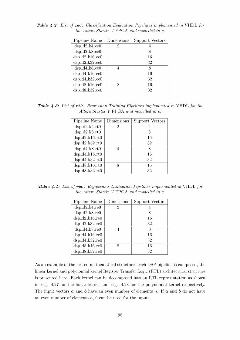
Table 4.2: List of ce0. Classification Evaluation Pipelines implemented in VHDL forthe Altera Startix V FPGA and modelled in c.
Pipeline Name Dimensions Support Vectors
dsp d2 k4 ce0 2 4dsp d2 k8 ce0 8dsp d2 k16 ce0 16dsp d2 k32 ce0 32
dsp d4 k8 ce0 4 8dsp d4 k16 ce0 16dsp d4 k32 ce0 32
dsp d8 k16 ce0 8 16dsp d8 k32 ce0 32
Table 4.3: List of rt0. Regression Training Pipelines implemented in VHDL for theAltera Startix V FPGA and modelled in c.
Pipeline Name Dimensions Support Vectors
dsp d2 k4 rt0 2 4dsp d2 k8 rt0 8dsp d2 k16 rt0 16dsp d2 k32 rt0 32
dsp d4 k8 rt0 4 8dsp d4 k16 rt0 16dsp d4 k32 rt0 32
dsp d8 k16 rt0 8 16dsp d8 k32 rt0 32
Table 4.4: List of re0. Regressions Evaluation Pipelines implemented in VHDL forthe Altera Startix V FPGA and modelled in c.
Pipeline Name Dimensions Support Vectors
dsp d2 k4 re0 2 4dsp d2 k8 re0 8dsp d2 k16 re0 16dsp d2 k32 re0 32
dsp d4 k8 re0 4 8dsp d4 k16 re0 16dsp d4 k32 re0 32
dsp d8 k16 re0 8 16dsp d8 k32 re0 32
As an example of the nested mathematical structures each DSP pipeline is composed, the
linear kernel and polynomial kernel Register Transfer Logic (RTL) architectural structure
is presented here. Each kernel can be decomposed into an RTL representation as shown
in Fig. 4.27 for the linear kernel and Fig. 4.28 for the polynomial kernel respectively.
The input vectors a and b have an even number of elements n. If a and b do not have
an even number of elements n, 0 can be used for the inputs.
95

a1 a2
an−1
b1 b2 bn−1
a • b
anbna3 b3 a4 b4
Figure 4.27: General RTL architectural structure of the linear kernel evaluationoperation.
a1 a2
an−1
b1 b2 bn−1
(a • b+ 1)2
1an
bna3 b3 a4 b4
Figure 4.28: General RTL architectural structure of the polynomial kernel evaluationoperation.
Each successive layer of RTL operations shown in Fig. 4.27 and Fig. 4.28 are implemented
as pipelined stages. Figure 4.29 illustrates the Linear kernel as a pipeline of staged-
instructions. Table 4.5 lists the Linear kernel pipeline instruction set and corresponding
implemented operations. Similarly, Figure 4.30 illustrates the Polynomial kernel as a
pipeline of staged-instructions. Table 4.6 lists the Polynomial kernel pipeline instruction
set and corresponding implemented operations. Stages shown in grey are drawn as one
single stage to simplify pipeline stage synchronisation. The grey stages are, however,
implemented as a series of stages where the number of stages in the series is a function
of input data dimensionality. The grey stage convention is used for all pipelines shown
throughout this section.
96

kvd0.
x1 xk
dot0.
dot0.
Stage 0.0
x1 xk
ψ1 ψk
ψ1 ψk
kmd0.
x1 xk
dot0.
dot0.
x1 xk
ψ11 ψkk
ψ11 ψkk
ψ(xi, xj) = xi • xj
x
Figure 4.29: Linear kernel pipeline.
Table 4.5: Linear kernel pipeline instruction overview.
⇒
x1 · x
...xk · x
kvd0.
ψ(xi, x)⇒ ψi×1 = ψ
⇒
x1 · x1 · · · x1 · xk
.... . .
...xk · x1 · · · xk · xk
kmd0.
ψ(xi, xj)⇒ ψi×j = ψ
Mathematical OperationInstruction
Listing 4.1 provides the VHDL required to instantiate the two linear kernel pipeline varia-
tions shown in Fig. 4.29 and Table 4.5. All DSP pipeline hardware stage implementations
presented in the this thesis utilise the same VHDL code structure as that shown in Listing
4.1 thus further DSP pipeline VHDL listings will not be included in this thesis. VHDL
Entitiy listings for each implemented pipeline, however, are presented in Appendix C.
97

Listing 4.1: VHDL code listing: Linear kernel pipeline stage.� �1 -- kvd0
2 kvd0_stage00 : FOR i IN 0 TO K_C -1 GENERATE
3 kvd0_stage00_dot0 : PROCESS( clk , rst , pipe_en_s(ST00_C) ) IS
4
5 VARIABLE kvd0_v : SIGNED( BITS_C -1 DOWNTO 0 );
6
7 BEGIN
8 IF rst = ’1’ THEN -- asynchronous reset
9 kvd0_s(i) <= ( OTHERS => ’0’ );
10 ELSIF RISING_EDGE( clk ) THEN
11 IF pipe_en_s(ST00_C) = ’1’ THEN
12 kvd0_v := RESIZE( (SIGNED( xv_s(D_C*i) ) * SIGNED( x_s (0) )), BITS_C ) +
RESIZE( (SIGNED( xv_s((D_C*i)+1) ) * SIGNED( x_s (1) )), BITS_C );
13 ELSE
14 kvd0_v := TO_SIGNED(0, BITS_C);
15 END IF;
16 kvd0_s(i) <= STD_LOGIC_VECTOR(kvd0_v);
17 END IF;
18
19 END PROCESS kvd0_stage00_dot0;
20 END GENERATE kvd0_stage00;
21
22 -- kmd0.
23 kmd0i_stage00 : FOR i IN 0 TO K_C -1 GENERATE
24 kmd0j_stage00 : FOR j IN 0 TO K_C -1 GENERATE
25 kmd0_stage00_dot0 : PROCESS( clk , rst , pipe_en_s(ST00_C) ) IS
26
27 VARIABLE kmd0_v : SIGNED( BITS_C -1 DOWNTO 0 );
28
29 BEGIN
30 IF rst = ’1’ THEN -- asynchronous reset
31 kmd0_s ((K_C*i)+j) <= ( OTHERS => ’0’ );
32 ELSIF RISING_EDGE( clk ) THEN
33 IF pipe_en_s(ST00_C) = ’1’ THEN
34 kmd0_v := RESIZE( (SIGNED( xv_s(D_C*i) ) * SIGNED( xv_s(D_C*j) )), BITS_C ) +
RESIZE( (SIGNED( xv_s((D_C*i)+1) ) * SIGNED( xv_s((D_C*j)+1) )), BITS_C
);
35 ELSE
36 kmd0_v := TO_SIGNED(0, BITS_C);
37 END IF;
38 kmd0_s ((K_C*i)+j) <= STD_LOGIC_VECTOR(kmd0_v);
39 END IF;
40
41 END PROCESS kmd0_stage00_dot0;
42 END GENERATE kmd0j_stage00;
43 END GENERATE kmd0i_stage00;� �
98

kmp2.
x1 xk
11 kk
kmp1.
+ c
+ c
dot0.
dot0.
Stage 0.0
Stage 1
Stage 2
·d
ψ11 ψkk
·d
kmp0.
x1 xk
ψ11 ψkk
kvp2.
x1 xk
1 k
kvp1.
+ c
+ c
dot0.
dot0.
·d
ψ1 ψk
·d
kvp0.
x1 xk
ψ1 ψk
1 k
1 k
1 k
11 kk
11 kk
11 kk
ψ(xi, xj) = (xi • xj + c)d
x
Figure 4.30: Polynomial kernel pipeline.
Table 4.6: Polynomial kernel pipeline instruction overview.
⇒
x1 · x
...xk · x
⇒
[x1 · x] + c...
[xk · x] + c
⇒
([x1 · x] + c)d
...
([xk · x] + c)d
=
ψ1
...ψk
= ψ
kvp1.
kvp0.
ψ(xi, x)⇒ ψi×1 = ψ
kvp2.
⇒
x1 · x1 · · · x1 · xk
.... . .
...xk · x1 · · · xk · xk
⇒
[x1 · x1] + c · · · [x1 · xk] + c...
. . ....
[xk · x1] + c · · · [xk · xk] + c
⇒
([x1 · x1] + c)d · · · ([x1 · xk] + c)d
.... . .
...
([xk · x1] + c)d · · · ([xk · xk] + c)d
=
ψ11 · · · ψ1k
.... . .
...ψk1 · · · ψkk
= ψ
kmp2.
kmp1.
kmp0.
ψ(xi, xj)⇒ ψi×j = ψ
Mathematical OperationInstruction
99

Figure 4.31 illustrates the ct0. classification training pipeline with the polynomial kernel.
Table 4.7 lists the ct0. classification training pipeline instruction set and corresponding
implemented operations.
ayv0.
α1 αk
a1 ak
kmp2.
x1 xk
11 kk
kmp1.
+1
+1
ctrhs2.
ctrhs1.
ctrhs0.
a1a1ψ11
akakψkk
α1y1
αkyk
11 kk
1 k
sum0.
sum0.
ctlhs0.
ct0.
sub0.
lhsrhs
sum0.
11 kk
11 kk
dot0.
dot0.
ψ11 ψkk a1a1 akak
sum0. sum0.
sum0.
11 kk
α1 αk1 k
lhsrhs
Stage 0.0
Stage 1
Stage 2
Stage 3
Stage 4.0
Stage 5.0
Stage 6
y1 yk
aat0.
akak
a1a1 akak
a1a1
a1 ak
·2
ψ11 ψkk
·211 kk
kmp0.
x1 xk α1 αky1 yk
ct0
ct0
Figure 4.31: ct0. Classification Training Pipeline.
100

Table 4.7: ct0. Classification Training Pipeline instruction overview.
⇒ aaT =[aaT
]i×i
=
a1a1 · · · a1ak...
. . ....
aka1 · · · akak
⇒k∑
i=1
αi = α1 + · · ·+ αk
⇒(
k∑
i=1
αi
)−(
1
2
k∑
i=1
k∑
j=1
αiαjyiyjψ(xi, xj)
)= ctlhs0.− ctrhs0.
⇒ a = [a] i×1 = a = [a] i×1 =
α1y1...
αkyk
=
a1...ak
⇒
x1 · x1 · · · x1 · xk
.... . .
...xk · x1 · · · xk · xk
⇒
[x1 · x1] + 1 · · · [x1 · xk] + 1...
. . ....
[xk · x1] + 1 · · · [xk · xk] + 1
⇒
([x1 · x1] + 1)2 · · · ([x1 · xk] + 1)2
.... . .
...([xk · x1] + 1)2 · · · ([xk · xk] + 1)2
=
ψ11 · · · ψ1k
.... . .
...ψk1 · · · ψkk
= ψ
kmp2.
kmp1.
kmp0.
⇒
a1a1ψ11 · · · a1akψ1k
.... . .
...aka1ψk1 · · · akakψkk
⇒
[a1a1ψ11] + · · ·+ [a1akψ1k]...
[aka1ψk1] + · · ·+ [akakψkk]
⇒ [a1a1ψ11] + · · ·+ [a1akψ1k] + · · ·+ [aka1ψk1] + · · ·+ [akakψkk]
aat0.
ayv0.
ct0.
ψ(xi, xj)⇒ ψi×j = ψ
1
2
k∑
i=1
k∑
j=1
αiαjyiyjψ(xi, xj) =1
2aTψ a
The 1/2 operation is a right-shift of 1 bit at the output of ctrhs0. stage.
ctrhs2.
ctrhs1.
ctrhs0.
ctlhs0.
Mathematical OperationInstruction
Figure 4.32 illustrates the ce0. classification evaluation pipeline with the polynomial
kernel. Table 4.8 lists the ce0. classification evaluation pipeline instruction set and
corresponding implemented operations.
101

α1 αk y1 yk
a1 ak
kvp2.
x1 xk
kvp1.
+1
·2
·2
lhs
cerhs0.
celhs0.
α1y1
αkyk
ce0.
sub0.
add0.
x
kvp2.
dot0.
dot0.
x1 xk
kvp1.
x+sv
kvp2.
dot0.
dot0.
x1 xk
1 k
kvp1.
x−sv
celhsp1.
a1 ak
celhsn1.
ψ1 ψk
rhsp1n1
+1+1
+1+1
+1
·2
·2
1 k 1 k
1 k1 k1 k
1 k 1 k 1 k
1 k 1 k
ψ1 ψk ψ1 ψk
dot0.
dot0.
a1 akψ1 ψk a1 akψ1 ψk
p1n1
lhs rhs
Stage 0.0
Stage 1
Stage 2
Stage 4.0
Stage 5
Stage 6
ψ1 ψk
·2
·21 k
kvp0. kvp0. kvp0. ayv0.
ce0
ce0
y1 ykx1 xk x1 xkx1 xkx−sv x+
sv x α1 αk
celhsn2.Stage 3 celhsp2.
akψk
a1ψ1
sum0.
sum0.
sum0.
sum0.
sum0.
sum0.
1 k 1 k 1 k
1 k 1 k 1 k
cerhs1.
akψk
a1ψ1
akψk
a1ψ1
Figure 4.32: ce0. Classification Evaluation Pipeline.
102

Table 4.8: ce0. Classification Evaluation DSP Pipeline instruction overview.
⇒k∑
i=1
αiyiψ(xi, x) = aT ψ = [a1ψ1] + · · ·+ [akψk]
⇒ a = [a] i×1 =
α1y1...
αkyk
=
a1...ak
⇒
x1 · x
...xk · x
⇒
[x1 · x] + 1...
[xk · x] + 1
kvp1.
kvp0.
ayv0.
1
2
(k∑
i=1
αiyiψ(xi, xsv+) +
k∑
i=1
αiyiψ(xi, xsv−)
)
kvp2.
⇒ celhsp1. + celhsn1.
The 1/2 operation is a right-shift of 1 bit at the output of celhs0. stage.
⇒k∑
i=1
αiyiψi − 1
2
(k∑
i=1
αiyiψi+ +
k∑
i=1
αiyiψi−
)= cerhs0. − celhs0.ce0.
⇒
([x1 · x] + 1)2
...([xk · x] + 1)2
=
ψ1
...ψk
= ψ
ψ(xi, x)⇒ ψi×1 = ψ
⇒
a1ψ1
...akψk
celhsp2.
celhsn2.
cerhs1.
celhsp1.
celhsn1.
cerhs0.
celhs0.
Mathematical OperationInstruction
Figure 4.33 illustrates the rt0. regression training pipeline with the polynomial kernel.
Table 4.9 lists the rt0. regression training pipeline instruction set and corresponding
implemented operations.
Figure 4.34 illustrates the re0. regression evaluation pipeline with the polynomial kernel.
Table 4.10 lists the re0. regression evaluation pipeline instruction set and corresponding
implemented operations.
103

ea0.
ea0
εea1
rtrhs1.
1 k
rhs
rtrhs0.
sub0.
sub0.
εk∑αi
sum0.
sum0.
sum0.
sum0.
α1α1ψ11
αkαkψkk
α•1 − α◦
1
α•k − α◦
k
+1
+1
α•1 + α◦
1
α•k + α◦
k
kmp2.
x1 xk
11 kk
dot0.
dot0.
kmp1. an0.
α•1 α•
k α◦1 α◦
k
yta0.
y1 ykα1 αk
yta0
rtrhs2.
α1α1 αkαk
11 kk
ea0
rtlhs0.
Stage 0.0
Stage 1
Stage 2
Stage 3
Stage 4.0
Stage 5.0
Stage 6
Stage 7
11 kk
11 kk
ψ11 ψkk
11 kk
1 k
rt0.
lhsrhs
lhs
ea1.
α1 αk
ea1
sum0.
sum0.
α1 αk α1 αk
ap0.
α•1 α•
k α◦1 α◦
k
rt0
yta0
x1 xk α•1 α•
k α◦1 α◦
ky1 yk
rt0
·2
·2
kmp0.
ψ11 ψkk
11 kk
αkαk
α1α1
aat0.
α1 αk α1 αk
α1α1 αkαk
yta1.
y1α1
1 k
1 k
sum0.
sum0.
ykαk
Figure 4.33: rt0. Regression Training Pipeline.
104

Table 4.9: rt0. Regression Training DSP Pipeline instruction overview.
⇒
x1 · x1 · · · x1 · xk
.... . .
...xk · x1 · · · xk · xk
⇒
[x1 · x1] + 1 · · · [x1 · xk] + 1...
. . ....
[xk · x1] + 1 · · · [xk · xk] + 1
⇒
([x1 · x1] + 1)2 · · · ([x1 · xk] + 1)2
.... . .
...([xk · x1] + 1)2 · · · ([xk · xk] + 1)2
=
ψ11 · · · ψ1k
.... . .
...ψk1 · · · ψkk
= ψ
kmp2.
kmp1.
kmp0.
ψ(xi, xj)⇒ ψi×j = ψ
⇒ α• + α◦ = αi×1 = αap0.
ααT =[ααT
]i×i
=
α1α1 · · · α1αk...
. . ....
αkα1 · · · αkαk
aat0.
⇒
α1α1ψ11 · · · α1αkψ1k
.... . .
...αkα1ψk1 · · · αkαkψkk
⇒
[α1α1ψ11] + · · ·+ [α1αkψ1k]...
[αkα1ψk1] + · · ·+ [αkαkψkk]
⇒ [α1α1ψ11] + · · ·+ [α1αkψ1k] + · · ·+ [αkα1ψk1] + · · ·+ [αkαkψkk]
1
2
k∑
i=1
k∑
j=1
αiαjψ(xi, xj) =1
2αTψ α
The 1/2 operation is a right-shift of 1 bit at the output of rtrhs0. stage.
k∑
j=1
yiαi − εk∑
i=1
αi = yT α− ε [α1 + · · ·+ αk]
⇒ α• − α◦ = αi×1 = α = αi×1 = α = αi×1 = αan0.
⇒ ε [α1 + · · ·+ αk]ea0.
⇒ α1 + · · ·+ αkea1.
⇒
y1α1
...ykαk
yta1.
⇒ [y1α1] + · · ·+ [ykαk]yta0.
⇒ [y1α1] + · · ·+ [ykαk]− ε [α1 + · · ·+ αk] = yta0.− ea0.
⇒(
k∑
i=1
yiαi − εk∑
i=1
αi
)−(
1
2
k∑
i=1
k∑
j=1
αiαjψ(xi, xj)
)= rtlhs0.− rtrhs0.rt0.
rtrhs2.
rtrhs1.
rtrhs0.
rtlhs0.
Mathematical OperationInstruction
105

an0.
α•1 α•
k α◦1 α◦
k
α1 αk
kmp2.
x1 xk
11 kk
kmp1.
+1
11 kk
+1
11 kk
·2
ψ11 ψkk
·2
rerhs3.
rerhs0.
α1ψ11
αkψkk
α•1 − α◦
1
11 kk
re0.
sub0.
lhs
α•k − α◦
k
x1 xk
1 k
kvp1.
ψ1 ψk
x
rerhs2.
α1ψ11−y1
αkψkk−yk
1 k
rhs
dot0.
dot0.
kvp2.
dot0.
dot0.
1 k
1 k
1 k
+1
+1
11 kk
·2
·2
ψ11 ψkk α1 αk
rerhs1.
sum0.
sum0.
sum0.
sum0.
11 kk
11 kk
11 kk
rhs
1 k
Stage 0.0
Stage 1
Stage 2
Stage 3
Stage 4
Stage 5.0
Stage 6.0
Stage 7
kvp0.kmp0.
re0
re0
x1 xk α•1 α•
k α◦1 α◦
ky1 yk x1 xkx
y1 yk
kvp0.
ψ1 ψkα1 αk
relhs1.
α1ψ1
αkψk
1 k
sum0.
sum0.
1 k
relhs0.
lhs
Figure 4.34: re0. Regression Evaluation Pipeline.
106

Table 4.10: re0. Regression Evaluation DSP Pipeline instruction overview.
Mathematical Operation
⇒
x1 · x
...xk · x
⇒
[x1 · x] + 1...
[xk · x] + 1
⇒
([x1 · x] + 1)2
...([xk · x] + 1)2
=
ψ1
...ψk
= ψ
kvp1.
kvp0.
ψ(xi, x)⇒ ψi×1 = ψ
Instruction
kvp2.
⇒
x1 · x1 · · · x1 · xk
.... . .
...xk · x1 · · · xk · xk
⇒
[x1 · x1] + 1 · · · [x1 · xk] + 1...
. . ....
[xk · x1] + 1 · · · [xk · xk] + 1
⇒
([x1 · x1] + 1)2 · · · ([x1 · xk] + 1)2
.... . .
...([xk · x1] + 1)2 · · · ([xk · xk] + 1)2
=
ψ11 · · · ψ1k
.... . .
...ψk1 · · · ψkk
= ψ
kmp2.
kmp1.
kmp0.
ψ(xi, xj)⇒ ψi×j = ψ
⇒ α• − α◦ = αi×1 = αan0.
k∑
i=1
αiψi = αT ψ
⇒
α1ψ1
...αkψk
⇒ [α1ψ1] + · · ·+ [αkψk]
1
k
k∑
i=1
k∑
j=1
αiψij − yj
⇒
α1ψ11 · · · α1ψ1k
.... . .
...αkψk1 · · · αkψkk
⇒
α1ψ11−y1 · · · α1ψ1k−yk
.... . .
...αkψk1−y1 · · · αkψkk−yk
⇒
[α1ψ11−y1] + · · ·+ [α1ψ1k−yk]...
[αkψk1−y1] + · · ·+ [αkψkk−yk]
The 1/k operation is a right-shift of k bits at the output of rerhs0. stage.
⇒ [α1ψ11−y1] + · · ·+ [α1ψ1k−yk] + · · ·+ [αkψk1−y1] + · · ·+ [αkψkk−yk]
⇒(
k∑
i=1
αiψi
)−(
1
k
k∑
i=1
k∑
j=1
αiψij − yj)
= relhs0. − rerhs0.re0.
relhs1.
relhs0.
rerhs3.
rerhs2.
rerhs1.
rerhs0.
107

4.4 Scientific Methodologies
This section presents scientific methodologies designed as part of this work, and, the data-
sets used in the application of these methodologies. The aims of the application of these
methodologies is twofold. Primarily the developed SVM DSP pipelines have been applied
to Rajkumar’s oil and pipeline domain application. Secondarily chaotic data-sets have
been used in various machine learning endeavours to investigate and explore the SVM
machine learning paradigm’s potential for use as a tool in non-linear and chaotic system’s
theory and time-series analysis.
Kernel PCA and k-means clustering tools of the MLPACK Machine Learning Library [100]
were used to reduce dimensionality. LIBSVM [101] was used to generate classification
and regression training sets and provide best-case SVM function evaluation experimental
benchmarks, and, inform further SVM DSP pipeline data-set application exploration.
4.4.1 Data-sets and Machine Learning Experimental Overview
Table 4.11 provides an overview of all data-sets and the SVM machine learning experi-
ments conducted as part of this work.
Table 4.11: SVM machine learning experiment overview.
Data-set
LADLorenz Attractor Data
Dimension d: 1, 2, 3, 4 and 8
MGADMackey-Glass Attractor Data
Dimension d: 1, 2, 4 and 8
ANNDANN Chaotic Oscillator Data
Dimension d: 1, 2, 4 and 8
LPDLegacy Oil & Gas Pipeline Data
Dimension d: 2, 4 and 8
Machine Learning Experimental Overview
SVM Classification SVM Regression
R-LPDArbitrary-Valued
Staircase Function
R-LADParameter Identification
R = 25, · · · , 33
R-MGADParameter Identification
τ = 17, · · · , 25
R-ANNDParameter Identification
D = 200, · · · , 3605 Class Classification
C-ANND
5 Class Classification
C-MGAD
5 Class Classification
C-LAD
C-LPD
5 Class Classification
Dimension d: 2, 4 and 8
Dimension d: 2, 4 and 8
Dimension d: 2, 4 and 8
Dimension d: 2, 4 and 8
Dimension d: 2, 4 and 8
Dimension d: 2, 4 and 8
Dimension d: 2, 4 and 8
Dimension d: 2, 4 and 8
Figure 4.35 provides an overview of the Legacy Oil and Gas Pipeline Data-Set (LPD) in
3-dimensional data-space rotated through 360 ◦ at 90 ◦ increments. Figure 4.36 provides
an overview of the Lorenz Attractor Data-Set (LAD) state-space response for system
parameters P = 10, B = 8/3, and (a) R = 25, with initial conditions x(0) = 0.0,
y(0) = −0.1, and z(0) = 9.0, through to (e) R = 33, with each previous system’s final
state as serving as initial conditions for the next. Figure 4.37 provides an overview of the
Mackey-Glass Attractor Data-Set (MGAD) 2-dimensional state-space response for system
108

parameters a = 0.2, b = 0.1, c = 10 and (a) τ = 17, increased at increments of 2 through
to (e) τ = 25. The state-space evolutions shown in Fig. 4.36 and Fig. 4.37 is illustrated as
a transition from green to blue. Figure 4.38 provides an overview of the Artificial Neural
Network Chaotic Oscillator Data-Set (ANND) time-series with the number of neurons
held constant at N = 10 and the delay-line length increased at increments of 40 from (a)
D = 200, through to (e) D = 360.
x3
x1
x2
x3
(a)
x3
x1
x2
x3
(b)
x3
x1
x2
x3
(c)
x3
x1
x2
x3
(d)
Figure 4.35: Legacy pipeline 3-dimensional data-space rotated through 360 ◦ at 90 ◦
increments.
109
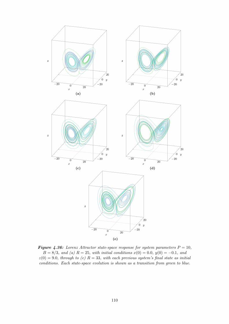
−200
20−20
0
20
z
x
y
z
(a)
−200
20−20
0
20
z
x
y
z
(b)
−200
20−20
0
20
z
x
y
z
(c)
−200
20−20
0
20
z
x
y
z
(d)
−200
20−20
0
20
z
x
y
z
(e)
Figure 4.36: Lorenz Attractor state-space response for system parameters P = 10,B = 8/3, and (a) R = 25, with initial conditions x(0) = 0.0, y(0) = −0.1, and
z(0) = 9.0, through to (e) R = 33, with each previous system’s final state as initialconditions. Each state-space evolution is shown as a transition from green to blue.
110
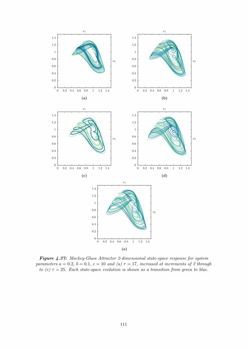
0
0.2
0.4
0.6
0.8
1
1.2
1.4
0 0.2 0.4 0.6 0.8 1 1.2 1.4
x2
x1
(a)
0
0.2
0.4
0.6
0.8
1
1.2
1.4
0 0.2 0.4 0.6 0.8 1 1.2 1.4
x2
x1
(b)
0
0.2
0.4
0.6
0.8
1
1.2
1.4
0 0.2 0.4 0.6 0.8 1 1.2 1.4
x2
x1
(c)
0
0.2
0.4
0.6
0.8
1
1.2
1.4
0 0.2 0.4 0.6 0.8 1 1.2 1.4
x2
x1
(d)
0
0.2
0.4
0.6
0.8
1
1.2
1.4
0 0.2 0.4 0.6 0.8 1 1.2 1.4
x2
x1
(e)
Figure 4.37: Mackey-Glass Attractor 2-dimensional state-space response for systemparameters a = 0.2, b = 0.1, c = 10 and (a) τ = 17, increased at increments of 2 through
to (e) τ = 25. Each state-space evolution is shown as a transition from green to blue.
111

−1
−0.5
0
0.5
1
0 200400
600800
1000
x[n]
n
(a)
−1
−0.5
0
0.5
1
0 200400
600800
1000
x[n]
n
(b)
−1
−0.5
0
0.5
1
0 200400
600800
1000
x[n]
n
(c)
−1
−0.5
0
0.5
1
0 200400
600800
1000
x[n]
n
(d)
−1
−0.5
0
0.5
1
0 200400
600800
1000
x[n]
n
(e)
Figure 4.38: ANN Chaotic Oscillator time-series with the number of neurons heldconstant at N = 10 and the delay-line length increased at increments of 40 from (a)
D = 200, through to (e) D = 360.
4.4.2 Data-set Processing and Application of SVM Systems
Figure 4.39 provides a generalised overview of each data-set’s data-flow through state-
space embedding and kernel Principal Component Analysis (PCA) dimension reduction
preprocessing strategies, training and data-set curation, SVM training strategies, and
finally the application of SVM function evaluation implementations.
112

Combined ExteriorPenalty & Barrier
FunctionOptimisation
LegacyPipelineDatad = 41
LPD LAD MGAD ANND
LorenzAttractor
Mackey-Glass
Attractor
ANNOscillator
Datad = 1, ,
32bit Floating-point Data Sets
d = 2, 4, 8
d = 1, 2, 3 d = 1· · · ∞
PCA & kPCADimension Reduction
Training Data
Test Data
Training & Test Data-set Curation
AugmentedLagrangeMultiplier
Optimisation
Brute-forceSearch Training
LIBSVM Trainingsvm-train
Support Vector Machine Training
ce0. re0.
FPGA Hardware
ce0. re0.
Software Models
32bit Floating-Point & 8bit Integer Scaling
State-Space Embedding
Reduced Dimension Data
Results
SVM Function Evaluation
Figure 4.39: Experimental Data-set Processing Overview.
4.4.2.1 Legacy Pipeline Data Methodology
The LPD data-set was inherited from Rajkumar’s original work [29]. The data-set in its
original raw form is a 41 dimensions data-space. The dimensionality of the data-set was
reduced using Kernel Principal Component Analysis (kPCA) with the polynomial kernel
to a 2 dimension data-space, a 3 dimension data-space, a 4 dimension data-space, and a
8 dimension data-space. The 3 dimension data-space achieved through the kPCA process
is shown in 4.35.
The reduced-dimension data-sets where then labelled appropriately and curated into
training and test data-sets. The data curation process applied an equal-probability ran-
dom sorting mechanic on each individual data-point into either a training data-set or a
test data-set. For SVM classification, C-LPD, five distinct training-test data-set pairs
were constructed; each training-test pair corresponded to a different -1 class data-cluster
assignment and all remaining clusters were assigned to the +1 class. For SVM regression,
R-LPD, each data-cluster was assigned an arbitrary enumerated label starting from 1
113

through to 5.
The training data-sets where then applied to each appropriate SVM classification and
SVM regression training strategies to obtain α Lagrangian coefficients and support vec-
tor pair SVM model data. Finally the trained SVM models and test data-sets were then
appropriately scaled and applied to the applicable SVM classification and SVM regression
function evaluation system implementations.
4.4.2.2 Chaotic Systems Data Methodology
The LAD data-set, the MGAD data-set, and the ANND data-set where generated through
the execution of custom software implementations of each respective system. Observing
the state-space evolutions shown in Fig. 4.36 and Fig. 4.37 and the time series shown in
Fig. 4.38.
Variations (over a small interval) in each of the the chaotic system’s underlying parame-
ters does little to change the general structure of the chaotic attractors and the subsequent
time-series and state-space evolution; this is clear by observing the state-space portraits
shown in Fig. 4.36 and Fig. 4.37 and the time series shown in Fig. 4.38 and noting
the very similar structures between each variation. This is after-all a key property of
chaotic systems - a sensitive dependence to initial conditions. In order to introduce a
more concrete relationship between each consecutive point along the state-space or time-
series evolution - that is to embed more of the subtle variations in response between
varied systems in each data-point, and, to increase the dissimilarities between each varied
system or to increase the varied system’s separation in feature-space, a 100 dimensional
state-space embedding was applied to each of the data-sets and their variations.
The dimensionality of the 100 dimension embedded state-space chaotic system data-sets
was reduced using kPCA with the polynomial kernel to a 2 dimension data-space, a 4 di-
mension data-space, and a 8 dimension data-space. The 3 dimension data-space achieved
through the kPCA process is shown in 4.35.
The reduced-dimension data-sets where then labelled appropriately and curated into
training and test data-sets. The data curation process applied an equal-probability ran-
dom sorting mechanic on each individual data-point into either a training data-set or a test
data-set. For SVM classification, C-LAD, C-MGAD, and C-ANND, five distinct training-
test data-set pairs, for each chaotic system data-set, were constructed; each training-test
pair corresponded to a different -1 class data-cluster assignment and all remaining clusters
were assigned to the +1 class. For SVM regression, R-LAD, R-MGAD, and R-ANND,
each data-cluster in each data-set was assigned a label reflecting the varied system pa-
rameter used to generate the original raw data. The Lorenz attractor system parameter
R was varied starting from R = 25 and increased at increments of 2 through to R = 33.
The Mackey-Glass attractor system parameter τ was varied starting from τ = 17 and in-
114

creased at increments of 2 through to τ = 25. Finally the ANN chaotic oscillator system
parameter D was varied starting from D = 200 and were increased at increments of 40
through to D = 360.
The training data-sets where then applied to each appropriate SVM classification and
SVM regression training strategies to obtain α Lagrangian coefficients and support vec-
tor pair SVM model data. Finally the trained SVM models and test data-sets were then
appropriately scaled and applied to the applicable SVM classification and SVM regression
function evaluation system implementations.
115

Chapter 5
Results
This chapter presents metrics gained through instrumentation and test measurement, and,
experimentally-obtained results pertaining to the SVM systems designed and developed
as part of the scope of this work and presented in Chapter 4. The chapter is organised
into three distinct sections; Section 5.1 DSP Results, Section 5.2 Electrical Results, and
Section 5.3 Machine Learning Results.
Section 5.1 DSP Results presents each pipeline architecture hardware implementation’s
FPGA resource utilisation, each pipeline architecture’s hardware and software model la-
tency and execution time, and each pipeline architecture’s instruction-per-cycle metrics.
Section 5.2 Electrical Results presents each pipeline architecture hardware implemen-
tation’s FPGA power consumption.
Section 5.3 Machine Learning Results presents results obtained through the application
of this work’s developed SVM systems with the four data-sets presented in Section 4.4.
These results are arranged into two subsections - Classification and Regression - each
dedicated to the machine learning experimental application of the same name as shown
in Table 4.11 and outlined in Section 4.4. Each subsection is then further organised into
sub-subsections by data-set: Legacy Pipeline Data (LPD), Lorenz Attractor Data (LAD),
Mackey-Glass Attractor Data (MGAD), and Artificial Neural Network Data (ANND).
116

5.1 DSP Results
All DSP pipeline architecture FPGA hardware implementations where compiled and
synthesised using Altera Quartus Prime [87] version 15.1 for an Altera Stratix V GS
5SGSMD5 FPGA device [102], [103]. All DSP pipeline architecture software model im-
plementations where compiled and executed on systems running the Arch Linux distri-
bution [94] employing Linux kernel version 4.6.2 using gcc version 6.1.1 [93]. All software
model executable metrics were collected using the Linux performance instrumentation
and profiling tool perf [104].
Table 5.1 provides an overview of the devices used for each FPGA hardware implementa-
tion and corresponding software model pipeline architecture implementation profiled and
reported in Section 5.1.
Table 5.1: Overview of devices used for each FPGA hardware implementation andcorresponding software model pipeline architecture implementation.
Device Manufacturer, Model, Clock CPU System
Label & Architecture Rate Cores RAM
FPGA Altera Stratix V GS 5SGSMD5-K2F40C2N (FPGA) 50 MHz - -
Core i7 Intel Core i7 6700K (x86 64) 4.00 GHz 8 16 GBCore 2 Intel Core 2 Duo P8600 (x86 64) 2.40 GHz 2 16 GBAtom Intel Atom N570 (x86 64) 1.66 GHz 4 2 GB
ARMv7 Broadcom BCM2836 - ARM Cortex-A7 (ARMv7) 900 MHz 4 1 GB
117

Table 5.2 shows each ct0. pipeline architecture FPGA hardware implementation stage-
count, and, latency tL with FPGA Master Clock Frequency clk of 50MHz. Table 5.3
shows FPGA resource utilisation for each ct0. pipeline architecture implementation
compiled and synthesised for the Altera Stratix V GS 5SGSMD5 FPGA device; rows
shown in grey were not synthesised due to DSP block resource requirements exceeding
available device DSP block resources.
Table 5.2: Pipeline architecture ct0. FPGA hardware implementation stage-count andlatency tL with master clock clk rate of 50MHz.
Pipeline ct0.
x Support Pipeline Pipeline
Dimension Vectors Stages Latency
(d) (k) tL (µs)
2 4 9 0.188 11 0.2216 13 0.2632 15 0.30
4 8 11 0.2216 13 0.2632 15 0.30
8 16 14 0.2832 16 0.32
Table 5.3: Pipeline architecture ct0. FPGA resource utilisation of Altera Stratix VGS 5SGSMD5 FPGA implementation.
Pipeline ct0.
x Support Combinational Logic DSPDimension Vectors LABs ALMs ALUTs Registers Blocks
(d) (k) (of 17,260) (of 172,600) Logic Route (of 345,200) (of 1,590)
2 4 298 1,221 2,442 497 2,399 728 1,105 4,714 9,360 1,944 9,492 27216 4,897 18,631 36,640 5,533 37,791 1,05632 - 55,327 56,073 - 110,651 2,048
4 8 1,153 4,714 9,360 1,897 9,491 30816 5,019 18,614 36,640 6,191 37,790 1,19232 - 55,328 56,072 - 110,653 3,104
8 16 5,814 20,529 39,224 8,033 42,687 1,46432 - 55,329 56,074 - 110,655 4,160
118

Table 5.4 shows each ct0. pipeline architecture FPGA hardware implementation and
corresponding software model latency / execution time tL performance metrics. Fig-
ure 5.1 illustrates each ct0. pipeline architecture FPGA hardware implementation and
corresponding software model latency / execution time tL performance metrics.
Table 5.4: Pipeline architecture ct0. FPGA hardware implementation andcorresponding software model latency / execution time tL performance metrics.
Pipeline ct0.
x Support Latency / Execution Time tL (µs)Dimension Vectors FPGA Software Model - Mean Execution Time
(d) (k) Hardware Core i7 Core 2 Atom ARMv7
2 4 0.18 287.70 484.36 1,839.73 3,388.578 0.22 582.89 476.48 1,872.66 3,418.5316 0.26 443.88 491.56 1,833.43 3,502.4832 0.30 473.90 510.58 2,020.39 3,622.26
4 8 0.22 698.00 484.01 1,868.89 3,426.5516 0.26 790.55 505.45 1,869.46 3,497.5932 0.30 705.75 528.13 1,937.39 3,663.93
8 16 0.28 899.89 495.09 1,946.31 3,524.3732 0.32 417.90 510.79 2,081.73 3,760.25
0.1
1
10
100
1000
10000
d2-k4
d2-k8
d2-k16
d2-k32
d4-k8
d4-k16
d4-k32
d8-k16
d8-k32
t L(µs)
Pipeline ct0.
FPGA Core i7 Core 2 Atom ARMv7
Figure 5.1: Pipeline architecture ct0. FPGA hardware implementation andcorresponding software model latency / execution time tL performance metrics.
119

Table 5.5 shows each ct0. pipeline architecture software model mean execution time
tL performance metric’s percentage standard deviation. Figure 5.2 illustrates each ct0.
pipeline architecture software model mean execution time tL performance metric’s per-
centage standard deviation.
Table 5.5: Pipeline architecture ct0. software model mean execution time tLperformance metric’s standard deviation (%).
Pipeline ct0.
x Support Software Model - Mean Execution Time
Dimension Vectors Standard Deviation (%)
(d) (k) Core i7 Core 2 Atom ARMv7
2 4 1.04 1.40 1.78 0.288 0.84 1.43 2.99 0.2616 1.14 1.46 1.65 0.3232 1.29 1.25 3.38 0.26
4 8 0.75 1.59 2.76 0.3316 0.77 1.23 2.31 0.2832 1.51 1.25 1.67 0.29
8 16 0.83 1.27 4.72 0.2832 3.01 1.36 5.36 0.26
0
2
4
6
8
10
d2-k4
d2-k8
d2-k16
d2-k32
d4-k8
d4-k16
d4-k32
d8-k16
d8-k32
StandardDeviation
(%)
Pipeline ct0.
Core i7 Core 2 Atom ARMv7
Figure 5.2: Pipeline architecture ct0. software model mean execution time tLperformance metric’s standard deviation (%).
120

Table 5.6 shows each ct0. pipeline architecture FPGA hardware implementation and
corresponding software model instructions-per-cycle performance metrics. Figure 5.3 il-
lustrates each ct0. pipeline architecture FPGA hardware implementation and corre-
sponding software model instructions-per-cycle performance metrics.
Table 5.6: Pipeline architecture ct0. FPGA hardware implementation andcorresponding software model instructions-per-cycle performance metrics.
Pipeline ct0.
x Support Instructions-per-CycleDimension Vectors FPGA Hardware Software Model - Mean IPC
(d) (k) DSP Delays Core i7 Core 2 Atom ARMv7
2 4 136 28 0.74 0.67 0.30 0.288 528 64 0.74 0.69 0.29 0.2816 2,080 144 0.75 0.69 0.31 0.2832 8,256 320 0.78 0.77 0.33 0.30
4 8 784 64 0.74 0.68 0.29 0.2816 3,104 144 0.76 0.71 0.31 0.2832 12,352 320 0.78 0.79 0.34 0.30
8 16 5,152 176 0.76 0.72 0.29 0.2932 20,544 384 0.78 0.83 0.31 0.31
0.1
1
10
100
1000
10000
d2-k4
d2-k8
d2-k16
d2-k32
d4-k8
d4-k16
d4-k32
d8-k16
d8-k32
Instructions-per-C
ycle
Pipeline ct0.
FPGA Core i7 Core 2 Atom ARMv7
Figure 5.3: Pipeline architecture ct0. FPGA hardware implementation andcorresponding software model instructions-per-cycle performance metrics.
121

Table 5.7 shows each ct0. pipeline architecture software model mean instructions-per-
cycle performance metric’s percentage standard deviation. Figure 5.4 illustrates each ct0.
pipeline architecture software model mean instructions-per-cycle performance metric’s
percentage standard deviation.
Table 5.7: Pipeline architecture ct0. software model mean instructions-per-cycleperformance metric’s standard deviation (%).
Pipeline ct0.
x Support Software Model Mean IPC
Dimension Vectors Standard Deviation (%)
(d) (k) Core i7 Core 2 Atom ARMv7
2 4 1.00 0.93 2.05 0.358 0.74 0.72 3.29 0.3116 1.00 0.81 1.55 0.3632 0.93 0.71 3.69 0.31
4 8 0.63 0.84 4.17 0.4116 0.61 0.75 2.11 0.3432 0.59 0.71 1.49 0.34
8 16 0.58 0.73 8.27 0.3332 0.78 0.64 9.47 0.30
0
2
4
6
8
10
d2-k4
d2-k8
d2-k16
d2-k32
d4-k8
d4-k16
d4-k32
d8-k16
d8-k32
IPC
StandardDeviation
(%)
Pipeline ct0.
Core i7 Core 2 Atom ARMv7
Figure 5.4: Pipeline architecture ct0. software model mean instructions-per-cycleperformance metric’s standard deviation (%).
122

Table 5.8 shows each ce0. pipeline architecture FPGA hardware implementation stage-
count, and, latency tL with FPGA Master Clock Frequency clk of 50MHz. Table 5.9
shows FPGA resource utilisation for each ce0. pipeline architecture implementation
compiled and synthesised for the Altera Stratix V GS 5SGSMD5 FPGA device.
Table 5.8: Pipeline architecture ce0. FPGA hardware implementation stage-count andlatency tL with master clock clk rate of 50MHz.
Pipeline ce0.
x Support Pipeline Pipeline
Dimension Vectors Stages Latency
(d) (k) tL (µs)
2 4 8 0.168 9 0.1816 10 0.2032 11 0.22
4 8 9 0.1816 10 0.2032 11 0.22
8 16 11 0.2232 12 0.24
Table 5.9: Pipeline architecture ce0. FPGA resource utilisation of Altera Stratix VGS 5SGSMD5 FPGA implementation.
Pipeline ce0.
x Support Combinational Logic DSPDimension Vectors LABs ALMs ALUTs Registers Blocks
(d) (k) (of 17,260) (of 172,600) Logic Route (of 345,200) (of 1,590)
2 4 128 760 1,520 204 1,492 408 305 1,548 3,095 364 2,982 8016 612 3,125 6,246 723 5,959 16032 1,234 6,275 12,549 1,297 11,911 320
4 8 305 1,548 3,095 387 2,981 10416 614 3,123 6,246 719 5,959 20832 1,212 6,275 12,549 1,339 11,911 416
8 16 862 3,724 7,158 1,482 7,688 30432 1,861 7,463 14,373 3,028 15,369 608
123
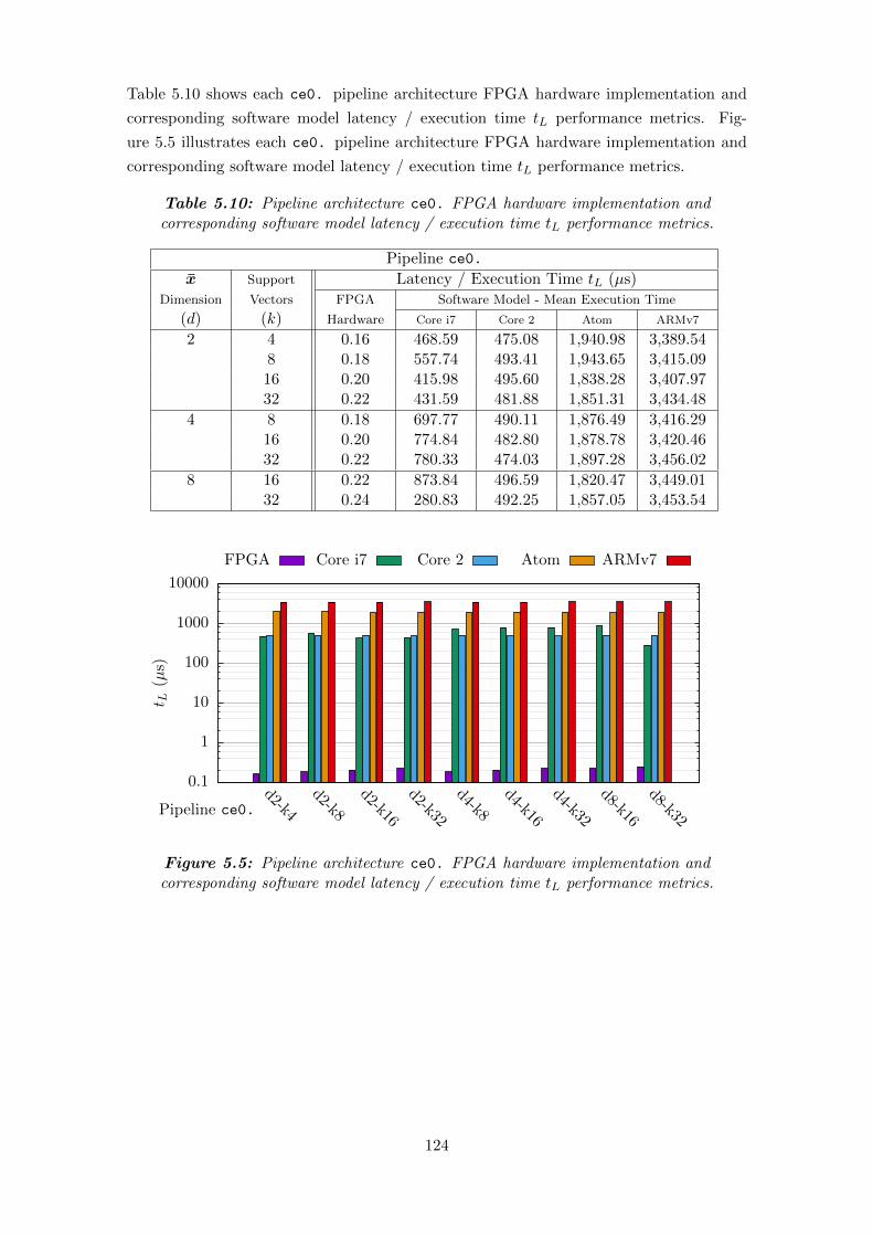
Table 5.10 shows each ce0. pipeline architecture FPGA hardware implementation and
corresponding software model latency / execution time tL performance metrics. Fig-
ure 5.5 illustrates each ce0. pipeline architecture FPGA hardware implementation and
corresponding software model latency / execution time tL performance metrics.
Table 5.10: Pipeline architecture ce0. FPGA hardware implementation andcorresponding software model latency / execution time tL performance metrics.
Pipeline ce0.
x Support Latency / Execution Time tL (µs)Dimension Vectors FPGA Software Model - Mean Execution Time
(d) (k) Hardware Core i7 Core 2 Atom ARMv7
2 4 0.16 468.59 475.08 1,940.98 3,389.548 0.18 557.74 493.41 1,943.65 3,415.0916 0.20 415.98 495.60 1,838.28 3,407.9732 0.22 431.59 481.88 1,851.31 3,434.48
4 8 0.18 697.77 490.11 1,876.49 3,416.2916 0.20 774.84 482.80 1,878.78 3,420.4632 0.22 780.33 474.03 1,897.28 3,456.02
8 16 0.22 873.84 496.59 1,820.47 3,449.0132 0.24 280.83 492.25 1,857.05 3,453.54
0.1
1
10
100
1000
10000
d2-k4
d2-k8
d2-k16
d2-k32
d4-k8
d4-k16
d4-k32
d8-k16
d8-k32
t L(µs)
Pipeline ce0.
FPGA Core i7 Core 2 Atom ARMv7
Figure 5.5: Pipeline architecture ce0. FPGA hardware implementation andcorresponding software model latency / execution time tL performance metrics.
124

Table 5.11 shows each ce0. pipeline architecture software model mean execution time
tL performance metric’s percentage standard deviation. Figure 5.6 illustrates each ce0.
pipeline architecture software model mean execution time tL performance metric’s per-
centage standard deviation.
Table 5.11: Pipeline architecture ce0. software model mean execution time tLperformance metric’s standard deviation (%).
Pipeline ce0.
x Support Software Model - Mean Execution Time
Dimension Vectors Standard Deviation (%)
(d) (k) Core i7 Core 2 Atom ARMv7
2 4 3.97 1.44 5.54 0.308 1.21 1.38 4.35 0.2716 1.67 1.60 1.76 0.2832 1.07 1.52 1.93 0.30
4 8 0.89 1.23 3.81 0.2616 0.76 1.18 3.44 0.2632 0.91 1.40 3.27 0.30
8 16 0.83 1.80 2.15 0.3232 1.07 1.36 2.75 0.29
0
2
4
6
8
10
d2-k4
d2-k8
d2-k16
d2-k32
d4-k8
d4-k16
d4-k32
d8-k16
d8-k32
StandardDeviation
(%)
Pipeline ce0.
Core i7 Core 2 Atom ARMv7
Figure 5.6: Pipeline architecture ce0. software model mean execution time tLperformance metric’s standard deviation (%).
125

Table 5.12 shows each ce0. pipeline architecture FPGA hardware implementation and
corresponding software model instructions-per-cycle performance metrics. Figure 5.7 il-
lustrates each ce0. pipeline architecture FPGA hardware implementation and corre-
sponding software model instructions-per-cycle performance metrics.
Table 5.12: Pipeline architecture ce0. FPGA hardware implementation andcorresponding software model instructions-per-cycle performance metrics.
Pipeline ce0.
x Support Instructions-per-CycleDimension Vectors FPGA Hardware Software Model - Mean IPC
(d) (k) DSP Delays Core i7 Core 2 Atom ARMv7
2 4 88 17 0.74 0.67 0.27 0.288 176 33 0.74 0.67 0.27 0.2816 352 65 0.74 0.68 0.30 0.2832 704 129 0.75 0.68 0.30 0.28
4 8 272 33 0.74 0.68 0.29 0.2816 544 65 0.74 0.68 0.29 0.2832 1,088 129 0.74 0.69 0.29 0.28
8 16 928 97 0.75 0.67 0.31 0.2832 1,856 193 0.74 0.69 0.30 0.28
0.1
1
10
100
1000
10000
d2-k4
d2-k8
d2-k16
d2-k32
d4-k8
d4-k16
d4-k32
d8-k16
d8-k32
Instructions-per-C
ycle
Pipeline ce0.
FPGA Core i7 Core 2 Atom ARMv7
Figure 5.7: Pipeline architecture ce0. FPGA hardware implementation andcorresponding software model instructions-per-cycle performance metrics.
126

Table 5.13 shows each ce0. pipeline architecture software model mean instructions-per-
cycle performance metric’s percentage standard deviation. Figure 5.8 illustrates each ce0.
pipeline architecture software model mean instructions-per-cycle performance metric’s
percentage standard deviation.
Table 5.13: Pipeline architecture ce0. software model mean instructions-per-cycleperformance metric’s standard deviation (%).
Pipeline ce0.
x Support Software Model Mean IPC
Dimension Vectors Standard Deviation (%)
(d) (k) Core i7 Core 2 Atom ARMv7
2 4 0.82 0.84 9.03 0.368 0.84 0.79 7.56 0.3216 1.03 0.79 2.03 0.3432 1.04 0.82 1.58 0.36
4 8 0.71 0.67 5.24 0.3116 0.61 0.79 3.30 0.3132 0.76 0.73 3.76 0.36
8 16 0.67 0.98 2.19 0.3832 1.03 0.70 2.87 0.35
0
2
4
6
8
10
d2-k4
d2-k8
d2-k16
d2-k32
d4-k8
d4-k16
d4-k32
d8-k16
d8-k32
IPC
StandardDeviation
(%)
Pipeline ce0.
Core i7 Core 2 Atom ARMv7
Figure 5.8: Pipeline architecture ce0. software model mean instructions-per-cycleperformance metric’s standard deviation (%).
127

Table 5.14 shows each rt0. pipeline architecture FPGA hardware implementation stage-
count, and, latency tL with FPGA Master Clock Frequency clk of 50MHz. Table 5.15
shows FPGA resource utilisation for each rt0. pipeline architecture implementation
compiled and synthesised for the Altera Stratix V GS 5SGSMD5 FPGA device; rows
shown in grey were not synthesised due to DSP block resource requirements exceeding
available device DSP block resources.
Table 5.14: Pipeline architecture rt0. FPGA hardware implementation stage-countand latency tL with master clock clk rate of 50MHz.
Pipeline rt0.
x Support Pipeline Pipeline
Dimension Vectors Stages Latency
(d) (k) tL (µs)
2 4 10 0.208 12 0.2416 14 0.2832 16 0.32
4 8 12 0.2416 14 0.2832 16 0.32
8 16 15 0.3032 17 0.34
Table 5.15: Pipeline architecture rt0. FPGA resource utilisation of Altera Stratix VGS 5SGSMD5 FPGA implementation.
Pipeline rt0.
x Support Combinational Logic DSPDimension Vectors LABs ALMs ALUTs Registers Blocks
(d) (k) (of 17,260) (of 172,600) Logic Route (of 345,200) (of 1,590)
2 4 219 1,071 2,087 316 2,192 568 809 4,045 8,008 850 8,161 20816 3,461 15,651 31,205 3,921 31,358 80032 - 71,664 57,373 - 143,327 1,873
4 8 813 4,044 8,008 909 8,161 24416 3,618 15,644 31,205 4,424 31,360 93632 - 71,672 57,388 - 143,342 2,929
8 16 4,639 17,547 33,783 6,694 36,249 1,20832 - 71,673 57,390 - 143,345 3,985
128

Table 5.16 shows each rt0. pipeline architecture FPGA hardware implementation and
corresponding software model latency / execution time tL performance metrics. Fig-
ure 5.9 illustrates each rt0. pipeline architecture FPGA hardware implementation and
corresponding software model latency / execution time tL performance metrics.
Table 5.16: Pipeline architecture rt0. FPGA hardware implementation andcorresponding software model latency / execution time tL performance metrics.
Pipeline rt0.
x Support Latency / Execution Time tL (µs)Dimension Vectors FPGA Software Model - Mean Execution Time
(d) (k) Hardware Core i7 Core 2 Atom ARMv7
2 4 0.20 358.84 485.00 1,767.10 3,415.298 0.24 615.85 478.83 1,831.73 3,422.0716 0.28 441.32 475.66 1,893.29 3,492.5832 0.32 466.77 510.11 1,908.30 3,639.97
4 8 0.24 811.61 486.31 1,790.73 3,443.5616 0.28 789.19 489.94 1,849.89 3,502.9832 0.32 760.88 522.30 2,015.19 3,654.13
8 16 0.30 258.32 500.69 1,939.84 3,514.5232 0.34 605.40 533.47 2,076.28 3,749.97
0.1
1
10
100
1000
10000
d2-k4
d2-k8
d2-k16
d2-k32
d4-k8
d4-k16
d4-k32
d8-k16
d8-k32
t L(µs)
Pipeline rt0.
FPGA Core i7 Core 2 Atom ARMv7
Figure 5.9: Pipeline architecture rt0. FPGA hardware implementation andcorresponding software model latency / execution time tL performance metrics.
129
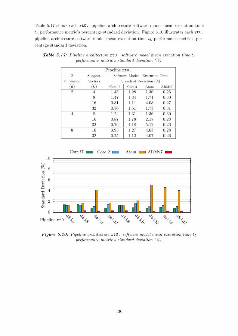
Table 5.17 shows each rt0. pipeline architecture software model mean execution time
tL performance metric’s percentage standard deviation. Figure 5.10 illustrates each rt0.
pipeline architecture software model mean execution time tL performance metric’s per-
centage standard deviation.
Table 5.17: Pipeline architecture rt0. software model mean execution time tLperformance metric’s standard deviation (%).
Pipeline rt0.
x Support Software Model - Execution Time
Dimension Vectors Standard Deviation (%)
(d) (k) Core i7 Core 2 Atom ARMv7
2 4 1.45 1.28 1.36 0.258 1.47 1.34 1.71 0.3016 0.81 1.11 4.08 0.2732 0.76 1.51 1.73 0.31
4 8 1.24 1.31 1.36 0.3016 0.87 1.78 2.17 0.2832 0.76 1.18 5.12 0.26
8 16 0.95 1.27 4.63 0.2832 0.75 1.12 4.07 0.26
0
2
4
6
8
10
d2-k4
d2-k8
d2-k16
d2-k32
d4-k8
d4-k16
d4-k32
d8-k16
d8-k32
StandardDeviation
(%)
Pipeline rt0.
Core i7 Core 2 Atom ARMv7
Figure 5.10: Pipeline architecture rt0. software model mean execution time tLperformance metric’s standard deviation (%).
130
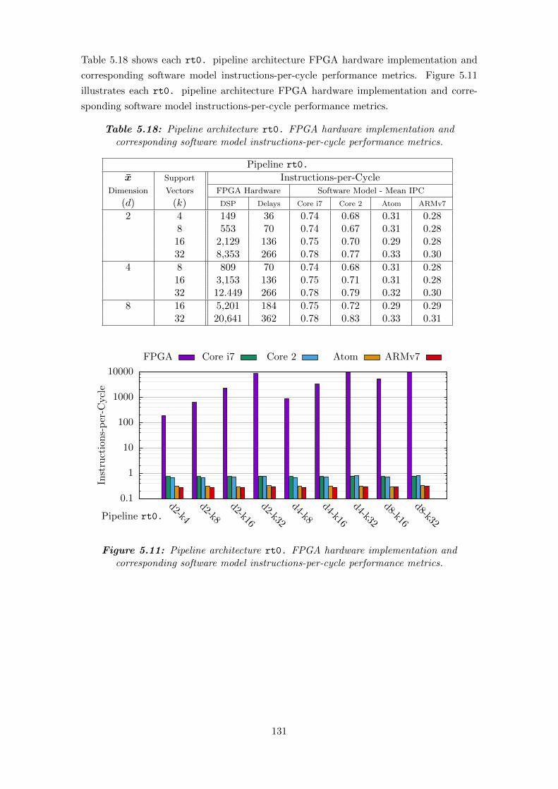
Table 5.18 shows each rt0. pipeline architecture FPGA hardware implementation and
corresponding software model instructions-per-cycle performance metrics. Figure 5.11
illustrates each rt0. pipeline architecture FPGA hardware implementation and corre-
sponding software model instructions-per-cycle performance metrics.
Table 5.18: Pipeline architecture rt0. FPGA hardware implementation andcorresponding software model instructions-per-cycle performance metrics.
Pipeline rt0.
x Support Instructions-per-CycleDimension Vectors FPGA Hardware Software Model - Mean IPC
(d) (k) DSP Delays Core i7 Core 2 Atom ARMv7
2 4 149 36 0.74 0.68 0.31 0.288 553 70 0.74 0.67 0.31 0.2816 2,129 136 0.75 0.70 0.29 0.2832 8,353 266 0.78 0.77 0.33 0.30
4 8 809 70 0.74 0.68 0.31 0.2816 3,153 136 0.75 0.71 0.31 0.2832 12.449 266 0.78 0.79 0.32 0.30
8 16 5,201 184 0.75 0.72 0.29 0.2932 20,641 362 0.78 0.83 0.33 0.31
0.1
1
10
100
1000
10000
d2-k4
d2-k8
d2-k16
d2-k32
d4-k8
d4-k16
d4-k32
d8-k16
d8-k32
Instructions-per-C
ycle
Pipeline rt0.
FPGA Core i7 Core 2 Atom ARMv7
Figure 5.11: Pipeline architecture rt0. FPGA hardware implementation andcorresponding software model instructions-per-cycle performance metrics.
131

Table 5.19 shows each rt0. pipeline architecture software model mean instructions-
per-cycle performance metric’s percentage standard deviation. Figure 5.12 illustrates
each rt0. pipeline architecture software model mean instructions-per-cycle performance
metric’s percentage standard deviation.
Table 5.19: Pipeline architecture rt0. software model mean instructions-per-cycleperformance metric’s standard deviation (%).
Pipeline rt0.
x Support Software Model Mean IPC
Dimension Vectors Standard Deviation (%)
(d) (k) Core i7 Core 2 Atom ARMv7
2 4 0.90 0.77 1.25 0.308 0.70 0.81 1.57 0.3716 0.70 0.66 5.75 0.3232 0.68 0.81 1.61 0.36
4 8 0.63 0.85 1.27 0.3616 0.67 0.84 2.58 0.3432 0.58 0.70 8.56 0.31
8 16 0.98 0.76 9.66 0.3532 0.55 0.68 5.59 0.30
0
2
4
6
8
10
d2-k4
d2-k8
d2-k16
d2-k32
d4-k8
d4-k16
d4-k32
d8-k16
d8-k32
IPC
StandardDeviation
(%)
Pipeline rt0.
Core i7 Core 2 Atom ARMv7
Figure 5.12: Pipeline architecture rt0. software model mean instructions-per-cycleperformance metric’s standard deviation (%).
132

Table 5.20 shows each re0. pipeline architecture FPGA hardware implementation stage-
count, and, latency tL with FPGA Master Clock Frequency clk of 50MHz. Table 5.21
shows FPGA resource utilisation for each re0. pipeline architecture implementation
compiled and synthesised for the Altera Stratix V GS 5SGSMD5 FPGA device; rows
shown in grey were not synthesised due to DSP block resource requirements exceeding
available device DSP block resources.
Table 5.20: Pipeline architecture re0. FPGA hardware implementation stage-countand latency tL with master clock clk rate of 50MHz.
Pipeline re0.
x Support Pipeline Pipeline
Dimension Vectors Stages Latency
(d) (k) tL (µs)
2 4 10 0.208 12 0.2416 14 0.2832 16 0.32
4 8 12 0.2416 14 0.2832 16 0.32
8 16 15 0.3032 17 0.34
Table 5.21: Pipeline architecture re0. FPGA resource utilisation of Altera Stratix VGS 5SGSMD5 FPGA implementation.
Pipeline re0.
x Support Combinational Logic DSPDimension Vectors LABs ALMs ALUTs Registers Blocks
(d) (k) (of 17,260) (of 172,600) Logic Route (of 345,200) (of 1,590)
2 4 269 1,485 2,867 338 3,041 548 947 5,389 10,518 914 10,815 18816 4,231 20,748 40,032 4,374 40,529 69632 - 84,022 96,259 - 168,042 1,772
4 8 973 5,386 10,518 1,031 10,815 23216 4,306 21,064 40,032 4,536 40,529 84832 - 84,022 96,259 - 168,042 2,892
8 16 5,217 23,005 42,921 7,490 46,004 1,15232 - 84,023 96,261 - 168,045 4,012
133

Table 5.22 shows each re0. pipeline architecture FPGA hardware implementation and
corresponding software model latency / execution time tL performance metrics. Figure
5.13 illustrates each re0. pipeline architecture FPGA hardware implementation and
corresponding software model latency / execution time tL performance metrics.
Table 5.22: Pipeline architecture re0. FPGA hardware implementation andcorresponding software model latency / execution time tL performance metrics.
Pipeline re0.
x Support Latency / Execution Time tL (µs)Dimension Vectors FPGA Software Model - Mean Execution Time
(d) (k) Hardware Core i7 Core 2 Atom ARMv7
2 4 0.20 290.61 485.82 1,812.11 3,387.958 0.24 588.58 476.98 1,886.88 3,438.0016 0.28 441.73 500.30 1,915.64 3,487.7932 0.32 471.09 501.00 1,962.67 3,647.48
4 8 0.24 701.52 510.49 1,757.86 3,463.7316 0.28 795.90 497.51 1,904.74 3,487.9932 0.32 764.98 521.76 2,009.64 3,654.92
8 16 0.30 298.66 494.90 1,872.30 3,537.6232 0.34 608.03 520.21 1,986.22 3,764.51
0.1
1
10
100
1000
10000
d2-k4
d2-k8
d2-k16
d2-k32
d4-k8
d4-k16
d4-k32
d8-k16
d8-k32
t L(µs)
Pipeline re0.
FPGA Core i7 Core 2 Atom ARMv7
Figure 5.13: Pipeline architecture re0. FPGA hardware implementation andcorresponding software model latency / execution time tL performance metrics.
134

Table 5.23 shows each re0. pipeline architecture software model mean execution time
tL performance metric’s percentage standard deviation. Figure 5.14 illustrates each re0.
pipeline architecture software model mean execution time tL performance metric’s per-
centage standard deviation.
Table 5.23: Pipeline architecture re0. software model mean execution time tLperformance metric’s standard deviation (%).
Pipeline re0.
x Support Software Model - Mean Execution Time
Dimension Vectors Standard Deviation (%)
(d) (k) Core i7 Core 2 Atom ARMv7
2 4 0.97 1.14 1.72 0.298 0.87 1.47 4.42 0.2816 0.90 1.22 3.20 0.2732 0.93 1.18 2.52 0.26
4 8 0.80 1.03 1.33 0.2716 0.92 1.12 2.70 0.2532 0.82 1.32 4.28 0.24
8 16 4.29 1.00 2.41 0.2632 0.72 1.49 2.57 0.24
0
2
4
6
8
10
d2-k4
d2-k8
d2-k16
d2-k32
d4-k8
d4-k16
d4-k32
d8-k16
d8-k32
StandardDeviation
(%)
Pipeline re0.
Core i7 Core 2 Atom ARMv7
Figure 5.14: Pipeline architecture re0. software model mean execution time tLperformance metric’s standard deviation (%).
135

Table 5.24 shows each re0. pipeline architecture FPGA hardware implementation and
corresponding software model instructions-per-cycle performance metrics. Figure 5.15
illustrates each re0. pipeline architecture FPGA hardware implementation and corre-
sponding software model instructions-per-cycle performance metrics.
Table 5.24: Pipeline architecture re0. FPGA hardware implementation andcorresponding software model instructions-per-cycle performance metrics.
Pipeline re0.
x Support Instructions-per-CycleDimension Vectors FPGA Hardware Software Model - Mean IPC
(d) (k) DSP Delays Core i7 Core 2 Atom ARMv7
2 4 160 38 0.73 0.68 0.30 0.288 576 75 0.74 0.68 0.29 0.2816 2,176 148 0.75 0.68 0.30 0.2932 8,448 293 0.78 0.77 0.33 0.30
4 8 864 75 0.74 0.68 0.31 0.2816 3,264 148 0.75 0.71 0.29 0.2932 12,672 293 0.78 0.79 0.31 0.30
8 16 5,568 196 0.75 0.71 0.30 0.2932 21,120 389 0.78 0.84 0.34 0.31
0.1
1
10
100
1000
10000
d2-k4
d2-k8
d2-k16
d2-k32
d4-k8
d4-k16
d4-k32
d8-k16
d8-k32
Instructions-per-C
ycle
Pipeline re0.
FPGA Core i7 Core 2 Atom ARMv7
Figure 5.15: Pipeline architecture re0. FPGA hardware implementation andcorresponding software model instructions-per-cycle performance metrics.
136

Table 5.25 shows each re0. pipeline architecture software model mean instructions-
per-cycle performance metric’s percentage standard deviation. Figure 5.16 illustrates
each re0. pipeline architecture software model mean instructions-per-cycle performance
metric’s percentage standard deviation.
Table 5.25: Pipeline architecture re0. software model mean instructions-per-cycleperformance metric’s standard deviation (%).
Pipeline re0.
x Support Software Model Mean IPC
Dimension Vectors Standard Deviation (%)
(d) (k) Core i7 Core 2 Atom ARMv7
2 4 1.00 0.72 1.52 0.358 0.72 0.77 5.57 0.3516 0.87 1.21 3.65 0.3132 0.76 0.73 2.38 0.30
4 8 0.71 0.75 1.39 0.3216 0.71 0.71 4.68 0.3032 0.61 0.71 9.68 0.28
8 16 0.99 0.84 4.08 0.3132 0.57 0.64 3.49 0.28
0
2
4
6
8
10
d2-k4
d2-k8
d2-k16
d2-k32
d4-k8
d4-k16
d4-k32
d8-k16
d8-k32
IPC
StandardDeviation
(%)
Pipeline re0.
Core i7 Core 2 Atom ARMv7
Figure 5.16: Pipeline architecture re0. software model mean instructions-per-cycleperformance metric’s standard deviation (%).
5.2 Electrical Results
Average power consumption was found by calculating the product of the applied DC
source voltage and measured DC current flowing into the Altera Stratix V GS 5SGSMD5
FPGA DSP development board running each DSP pipeline implementation with pipeline
enable en rate of 20 kHz, or 50 MHz, applied to the pipeline circuit.
Idle-state power consumption of an Altera Stratix V GS 5SGSMD5 FPGA DSP develop-
137

ment board, running a trivial clock and synchronous-reset process hardware implementa-
tion, was calculated to be 10.75 W.
Table 5.26 shows the average power consumption of each Altera Stratix V GS 5SGSMD5
FPGA DSP development board ct0. pipeline architecture implementation with pipeline
enable en rate of 20 kHz and 50 MHz. Figure 5.17 illustrates the average power con-
sumption of each Altera Stratix V GS 5SGSMD5 FPGA DSP development board ct0.
pipeline architecture implementation with pipeline enable en rate of 20 kHz and 50 MHz.
Table 5.26: Pipeline architecture ct0. average power consumption of each AlteraStratix V GS 5SGSMD5 FPGA DSP development board implementation with pipeline
enable en rate of 20 kHz and 50 MHz.
Pipeline ct0.
x Support Power (W)
Dimension Vectors @ pipeline en rate:
(d) (k) 20 kHz 50 MHz
2 4 10.68 11.198 11.02 11.2116 11.10 11.4832 - -
4 8 10.91 10.8916 10.86 11.2832 - -
8 16 10.99 11.3132 - -
10
10.5
11
11.5
12
d2-k4
d2-k8
d2-k16
d2-k32
d4-k8
d4-k16
d4-k32
d8-k16
d8-k32
Pow
er(W
)
Pipeline ct0.
20 kHz 50 MHz
Figure 5.17: Pipeline architecture ct0. average power consumption of each AlteraStratix V GS 5SGSMD5 FPGA DSP development board implementation with pipeline
enable en rate of 20 kHz and 50 MHz.
138

Table 5.27 shows the average power consumption of each Altera Stratix V GS 5SGSMD5
FPGA DSP development board ce0. pipeline architecture implementation with pipeline
enable en rate of 20 kHz and 50 MHz. Figure 5.18 illustrates the average power con-
sumption of each Altera Stratix V GS 5SGSMD5 FPGA DSP development board ce0.
pipeline architecture implementation with pipeline enable en rate of 20 kHz and 50 MHz.
Table 5.27: Pipeline architecture ce0. average power consumption of each AlteraStratix V GS 5SGSMD5 FPGA DSP development board implementation with pipeline
enable en rate of 20 kHz and 50 MHz.
Pipeline ce0.
x Support Power (W)
Dimension Vectors @ pipeline en rate:
(d) (k) 20 kHz 50 MHz
2 4 10.80 10.858 10.66 10.9116 11.05 10.8732 11.14 11.01
4 8 10.85 10.7616 10.91 11.3032 11.12 10.76
8 16 10.78 10.8732 10.87 10.72
10
10.5
11
11.5
12
d2-k4
d2-k8
d2-k16
d2-k32
d4-k8
d4-k16
d4-k32
d8-k16
d8-k32
Pow
er(W
)
Pipeline ce0.
20 kHz 50 MHz
Figure 5.18: Pipeline architecture ce0. average power consumption of each AlteraStratix V GS 5SGSMD5 FPGA DSP development board implementation with pipeline
enable en rate of 20 kHz and 50 MHz.
139
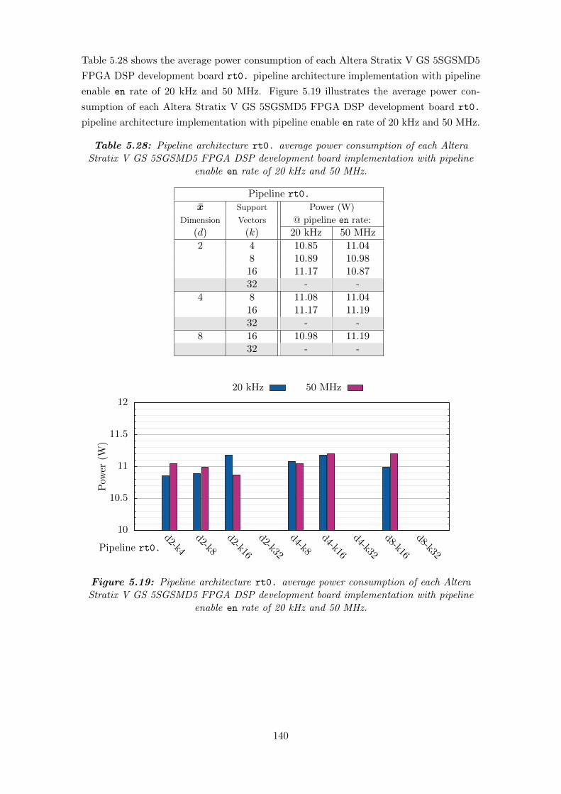
Table 5.28 shows the average power consumption of each Altera Stratix V GS 5SGSMD5
FPGA DSP development board rt0. pipeline architecture implementation with pipeline
enable en rate of 20 kHz and 50 MHz. Figure 5.19 illustrates the average power con-
sumption of each Altera Stratix V GS 5SGSMD5 FPGA DSP development board rt0.
pipeline architecture implementation with pipeline enable en rate of 20 kHz and 50 MHz.
Table 5.28: Pipeline architecture rt0. average power consumption of each AlteraStratix V GS 5SGSMD5 FPGA DSP development board implementation with pipeline
enable en rate of 20 kHz and 50 MHz.
Pipeline rt0.
x Support Power (W)
Dimension Vectors @ pipeline en rate:
(d) (k) 20 kHz 50 MHz
2 4 10.85 11.048 10.89 10.9816 11.17 10.8732 - -
4 8 11.08 11.0416 11.17 11.1932 - -
8 16 10.98 11.1932 - -
10
10.5
11
11.5
12
d2-k4
d2-k8
d2-k16
d2-k32
d4-k8
d4-k16
d4-k32
d8-k16
d8-k32
Pow
er(W
)
Pipeline rt0.
20 kHz 50 MHz
Figure 5.19: Pipeline architecture rt0. average power consumption of each AlteraStratix V GS 5SGSMD5 FPGA DSP development board implementation with pipeline
enable en rate of 20 kHz and 50 MHz.
140

Table 5.29 shows the average power consumption of each Altera Stratix V GS 5SGSMD5
FPGA DSP development board re0. pipeline architecture implementation with pipeline
enable en rate of 20 kHz and 50 MHz. Figure 5.20 illustrates the average power con-
sumption of each Altera Stratix V GS 5SGSMD5 FPGA DSP development board re0.
pipeline architecture implementation with pipeline enable en rate of 20 kHz and 50 MHz.
Table 5.29: Pipeline architecture re0. average power consumption of each AlteraStratix V GS 5SGSMD5 FPGA DSP development board implementation with pipeline
enable en rate of 20 kHz and 50 MHz.
Pipeline re0.
x Support Power (W)
Dimension Vectors @ pipeline en rate:
(d) (k) 20 kHz 50 MHz
2 4 10.98 11.148 11.06 11.1416 11.25 11.6732 - -
4 8 11.06 11.5016 11.12 11.3732 - -
8 16 11.08 11.3332 - -
10
10.5
11
11.5
12
d2-k4
d2-k8
d2-k16
d2-k32
d4-k8
d4-k16
d4-k32
d8-k16
d8-k32
Pow
er(W
)
Pipeline re0.
20 kHz 50 MHz
Figure 5.20: Pipeline architecture re0. average power consumption of each AlteraStratix V GS 5SGSMD5 FPGA DSP development board implementation with pipeline
enable en rate of 20 kHz and 50 MHz.
141

5.3 Machine Learning Results
The results in this section are arranged into subsections pertaining to the Classification
and Regression machine learning experimental applications as shown in Table 4.11 and
outlined in Section 4.4. Each subsection is further organised by data-set: Legacy Pipeline
Data (LPD), Lorenz Attractor Data (LAD), Mackey-Glass Attractor Data (MGAD), and
Artificial Neural Network Data (ANND).
5.3.1 SVM Classification Results
This section presents the optimal SVM classification results obtained through the appli-
cation of the scientific methodologies with the four data-sets described in Section 4.4.
The Linear kernel, Polynomial kernel, Radial Basis Function / Gaussian kernel, and Sig-
moid kernel were applied with LIBSVM, however optimal results where obtained with the
Polynomial kernel and thus only these results are reproduced here.
SVM classification results derived from the application of the brute-force training tech-
nique are absent from this section due to technological limitations when applied to non-
trivial data-sets. Similarly combined exterior penalty function and barrier function op-
timisation method and the augmented Lagrange multiplier optimisation method is not
shown due to unacceptably poor performance in both function and resulting classification
accuracies. The failures of these proposed SVM classification training techniques will be
discussed in Chapter 6.
SVM classification results using the DSP pipelines outlined in Section 4.3 are only shown
when a LIBSVM-trained SVM classification model support vector set does not exceed the
technical limitations of the ce0. DSP pipeline architecture variations.
5.3.1.1 C-LPD
Optimal results obtained for SVM classification applied to the LPD data-set using LIB-
SVM training and function evaluation routines and utilising the polynomial kernel are
shown in Table 5.30. Optimal results obtained for SVM classification applied to the LPD
data-set using LIBSVM training and ce0. DSP pipeline function evaluation are shown
in Table 5.31.
142
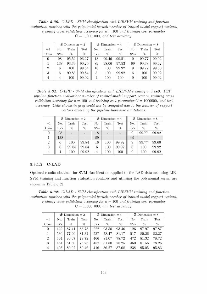
Table 5.30: C-LPD - SVM classification with LIBSVM training and functionevaluation routines with the polynomial kernel; number of trained-model support vectors,
training cross validation accuracy for n = 100 and training cost parameterC = 1, 000, 000, and test accuracy.
x Dimension = 2 x Dimension = 4 x Dimension = 8
+1 No. Train Test No. Train Test No. Train Test
Class SVs % % SVs % % SVs % %
0 98 95.52 96.27 18 99.46 99.51 9 99.77 99.921 138 93.39 90.20 89 98.06 97.53 69 99.38 99.422 6 100 99.84 16 100 99.92 9 99.77 99.603 6 99.85 99.84 5 100 99.92 6 100 99.924 4 100 99.92 4 100 100 9 100 99.92
Table 5.31: C-LPD - SVM classification with LIBSVM training and ce0. DSPpipeline function evaluation; number of trained-model support vectors, training crossvalidation accuracy for n = 100 and training cost parameter C = 1000000, and testaccuracy. Cells shown in grey could not be computed due to the number of support
vectors exceeding the pipeline hardware limitations.
x Dimension = 2 x Dimension = 4 x Dimension = 8
+1 No. Train Test No. Train Test No. Train Test
Class SVs % % SVs % % SVs % %
0 98 - - 18 - - 9 99.77 99.921 138 - - 89 - - 69 - -2 6 100 99.84 16 100 99.92 9 99.77 99.603 6 99.85 99.84 5 100 99.92 6 100 99.924 4 100 99.92 4 100 100 9 100 99.92
5.3.1.2 C-LAD
Optimal results obtained for SVM classification applied to the LAD data-set using LIB-
SVM training and function evaluation routines and utilising the polynomial kernel are
shown in Table 5.32.
Table 5.32: C-LAD - SVM classification with LIBSVM training and functionevaluation routines with the polynomial kernel; number of trained-model support vectors,
training cross validation accuracy for n = 100 and training cost parameterC = 1, 000, 000, and test accuracy.
x Dimension = 2 x Dimension = 4 x Dimension = 8
+1 No. Train Test No. Train Test No. Train Test
Class SVs % % SVs % % SVs % %
0 422 87.41 88.73 222 93.50 93.46 126 97.97 97.871 530 77.90 81.32 537 78.47 81.17 517 80.26 82.272 464 80.67 78.72 466 81.07 78.72 472 81.32 78.723 454 81.80 78.25 457 81.80 78.25 460 81.56 78.264 493 80.02 80.46 416 86.27 87.08 238 95.05 95.83
143

5.3.1.3 C-MGAD
Optimal results obtained for SVM classification applied to the MGAD data-set using
LIBSVM training and function evaluation routines and utilising the polynomial kernel
are shown in Table 5.33.
Table 5.33: C-MGAD - SVM classification with LIBSVM training and functionevaluation routines with the polynomial kernel; number of trained-model support vectors,
training cross validation accuracy for n = 100 and training cost parameterC = 1, 000, 000, and test accuracy.
x Dimension = 2 x Dimension = 4 x Dimension = 8
+1 No. Train Test No. Train Test No. Train Test
Class SVs % % SVs % % SVs % %
0 519 78.64 80.64 522 79.36 80.64 518 80.48 82.151 533 78.80 80.80 527 79.20 80.80 534 79.20 80.802 516 78.72 79.92 511 80.16 79.92 507 80.08 79.923 511 78.55 80.08 513 79.92 80.08 510 79.44 79.924 468 80.48 78.57 473 81.45 78.57 480 81.53 78.41
5.3.1.4 C-ANND
Optimal results obtained for SVM classification applied to the ANND data-set using
LIBSVM training and function evaluation routines and utilising the polynomial kernel is
shown in Table 5.34.
Table 5.34: C-ANND - SVM classification with LIBSVM training and functionevaluation routines with the polynomial kernel; number of trained-model support vectors,
training cross validation accuracy for n = 100 and training cost parameterC = 1, 000, 000, and test accuracy.
x Dimension = 2 x Dimension = 4 x Dimension = 8
+1 No. Train Test No. Train Test No. Train Test
Class SVs % % SVs % % SVs % %
0 205 92.44 93.23 191 94.21 94.59 192 94.21 94.431 329 89.39 89.41 44 98.47 98.73 35 98.88 98.572 426 83.84 84.32 373 85.69 86.31 320 88.67 88.223 199 93.41 94.75 136 95.10 95.62 72 97.67 97.214 404 84.00 84.71 383 84.81 84.71 387 84.33 85.27
5.3.2 SVM Regression Results
This section presents the optimal SVM regression results obtained through the applica-
tion of the scientific methodologies with the four data-sets described in Section 4.4. The
Linear kernel, Polynomial kernel, Radial Basis Function / Gaussian kernel, and Sigmoid
kernel were applied with LIBSVM, however optimal results where obtained with the Poly-
nomial kernel and thus only these results are reproduced here.
As with their SVM classification training counterparts SVM regression training efforts
using the combined exterior penalty function and barrier function optimisation method
144
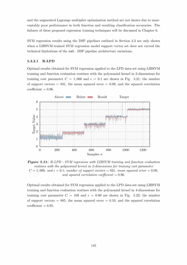
and the augmented Lagrange multiplier optimisation method are not shown due to unac-
ceptably poor performance in both function and resulting classification accuracies. The
failures of these proposed regression training techniques will be discussed in Chapter 6.
SVM regression results using the DSP pipelines outlined in Section 4.3 are only shown
when a LIBSVM-trained SVM regression model support vector set does not exceed the
technical limitations of the re0. DSP pipeline architecture variations.
5.3.2.1 R-LPD
Optimal results obtained for SVM regression applied to the LPD data-set using LIBSVM
training and function evaluation routines with the polynomial kernel in 2-dimensions for
training cost parameter C = 1, 000 and ε = 0.1 are shown in Fig. 5.21; the number
of support vectors = 831, the mean squared error = 0.09, and the squared correlation
coefficient = 0.96.
0
1
2
3
4
5
6
0 200 400 600 800 1000 1200
TargetValue
Samples n
Above Below Result Target
Figure 5.21: R-LPD - SVM regression with LIBSVM training and function evaluationroutines with the polynomial kernel in 2-dimensions for training cost parameter
C = 1, 000, and ε = 0.1; number of support vectors = 831, mean squared error = 0.09,and squared correlation coefficient = 0.96.
Optimal results obtained for SVM regression applied to the LPD data-set using LIBSVM
training and function evaluation routines with the polynomial kernel in 4-dimensions for
training cost parameter C = 108 and ε = 0.09 are shown in Fig. 5.22; the number
of support vectors = 885, the mean squared error = 0.10, and the squared correlation
coefficient = 0.95.
145

0
1
2
3
4
5
6
0 200 400 600 800 1000 1200
Target
Value
Samples n
Above Below Result Target
Figure 5.22: R-LPD - SVM regression with LIBSVM training and function evaluationroutines with the polynomial kernel in 4-dimensions for training cost parameter
C = 108, and ε = 0.09; number of support vectors = 885, mean squared error = 0.10,and squared correlation coefficient = 0.95.
Optimal results obtained for SVM regression applied to only two data-clusters of the
LPD data-set using LIBSVM training and re0. DSP pipeline function evaluation in 4-
dimensions for training cost parameter C = 1000 and ε = 0.1 are shown in Fig. 5.23;
the number of support vectors = 31, the mean squared error = 0.00, and the squared
correlation coefficient = 0.99. Using only two data-clusters of the LPD data-set the
trained model support vector count was kept within the technical limitations of of re0.
DSP pipeline.
3.5
4
4.5
5
5.5
0 50 100 150 200 250 300 350 400 450
TargetValue
Samples n
Above Below Result Target
Figure 5.23: R-LPD - SVM regression with LIBSVM training (using to only twodata-clusters of data-set to limit support vector count) and re0. DSP pipeline functionevaluation in 4-dimensions for training cost parameter C = 1000, and ε = 0.1; numberof support vectors = 31, mean squared error = 0.00, and squared correlation coefficient
= 0.99.
146

Optimal results obtained for SVM regression applied to the LPD data-set using LIBSVM
training and function evaluation routines with the polynomial kernel in 8-dimensions for
training cost parameter C = 6, and ε = 0.1 are shown in Fig. 5.24; the number of support
vectors = 806, the mean squared error = 0.10, and the squared correlation coefficient
= 0.96.
0
1
2
3
4
5
6
0 200 400 600 800 1000 1200
Target
Value
Samples n
Above Below Result Target
Figure 5.24: R-LPD - SVM regression with LIBSVM training and function evaluationroutines with the polynomial kernel in 8-dimensions for training cost parameter C = 6,and ε = 0.1; number of support vectors = 806, mean squared error = 0.10, and squared
correlation coefficient = 0.96.
Optimal results obtained for SVM regression applied to only two data-clusters of the
LPD data-set using LIBSVM training and re0. DSP pipeline function evaluation in
8-dimensions for training cost parameter C = 400 and ε = 0.1 are shown in Fig. 5.25;
the number of support vectors = 30, the mean squared error = 0.00, and the squared
correlation coefficient = 0.99. Using only two data-clusters of the LPD data-set the
trained model support vector count was kept within the technical limitations of of re0.
DSP pipeline.
147

3.5
4
4.5
5
5.5
0 50 100 150 200 250 300 350 400 450
Target
Value
Samples n
Above Below Result Target
Figure 5.25: R-LPD - SVM regression with LIBSVM training (using to only twodata-clusters of data-set to limit support vector count) and re0. DSP pipeline functionevaluation in 8-dimensions for training cost parameter C = 400, and ε = 0.1; number of
support vectors = 30, mean squared error = 0.00, and squared correlation coefficient= 0.99.
5.3.2.2 R-LAD
Optimal results obtained for SVM regression applied to the LAD data-set using LIBSVM
training and function evaluation routines with the polynomial kernel in 2-dimensions for
training cost parameter C = 1, 000, 000, and ε = 0.1 are shown in Fig. 5.26; the number
of support vectors = 1, 229, the mean squared error = 7.07, and the squared correlation
coefficient = 0.11.
24
26
28
30
32
34
0 200 400 600 800 1000 1200
R
Time t
Above Below Result Target
Figure 5.26: R-LAD - SVM regression with LIBSVM training and function evaluationroutines with the polynomial kernel in 2-dimensions for training cost parameter
C = 1, 000, 000, and ε = 0.1; number of support vectors = 1, 229, mean squared error= 7.07, and squared correlation coefficient = 0.11.
Optimal results obtained for SVM regression applied to the LAD data-set using LIBSVM
148

training and function evaluation routines with the polynomial kernel in 4-dimensions for
training cost parameter C = 1, 000, 000, and ε = 0.1 are shown in Fig. 5.27; the number
of support vectors = 1, 213, the mean squared error = 4.09, and the squared correlation
coefficient = 0.51.
24
26
28
30
32
34
0 200 400 600 800 1000 1200
R
Time t
Above Below Result Target
Figure 5.27: R-LAD - SVM regression with LIBSVM training and function evaluationroutines with the polynomial kernel in 4-dimensions for training cost parameter
C = 1, 000, 000, and ε = 0.1; number of support vectors = 1, 213, mean squared error= 4.09, and squared correlation coefficient = 0.51.
Optimal results obtained for SVM regression applied to the LAD data-set using LIBSVM
training and function evaluation routines with the polynomial kernel in 8-dimensions for
training cost parameter C = 1, 000, 000, and ε = 0.1 are shown in Fig. 5.28; the number
of support vectors = 1, 223, the mean squared error = 2.09, and the squared correlation
coefficient = 0.75.
149

24
26
28
30
32
34
0 200 400 600 800 1000 1200
R
Time t
Above Below Result Target
Figure 5.28: R-LAD - SVM regression with LIBSVM training and function evaluationroutines with the polynomial kernel in 8-dimensions for training cost parameter
C = 1, 000, 000, and ε = 0.1; number of support vectors = 1, 223, mean squared error= 2.09, and squared correlation coefficient = 0.75.
5.3.2.3 R-MGAD
Optimal results obtained for SVM regression applied to the MGAD data-set using LIB-
SVM training and function evaluation routines with the polynomial kernel in 2-dimensions
for training cost parameter C = 1, 000, 000, and ε = 0.1 are shown in Fig. 5.29; the number
of support vectors = 1, 195, the mean squared error = 8.17, and the squared correlation
coefficient = 0.01.
16
18
20
22
24
26
0 200 400 600 800 1000 1200
τ
Time t
Above Below Result Target
Figure 5.29: R-MGAD - SVM regression with LIBSVM training and functionevaluation routines with the polynomial kernel in 2-dimensions for training cost
parameter C = 1, 000, 000, and ε = 0.1; number of support vectors = 1, 195, meansquared error = 8.17, and squared correlation coefficient = 0.01.
Optimal results obtained for SVM regression applied to the MGAD data-set using LIB-
150
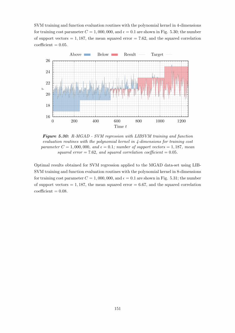
SVM training and function evaluation routines with the polynomial kernel in 4-dimensions
for training cost parameter C = 1, 000, 000, and ε = 0.1 are shown in Fig. 5.30; the number
of support vectors = 1, 187, the mean squared error = 7.62, and the squared correlation
coefficient = 0.05.
16
18
20
22
24
26
0 200 400 600 800 1000 1200
τ
Time t
Above Below Result Target
Figure 5.30: R-MGAD - SVM regression with LIBSVM training and functionevaluation routines with the polynomial kernel in 4-dimensions for training cost
parameter C = 1, 000, 000, and ε = 0.1; number of support vectors = 1, 187, meansquared error = 7.62, and squared correlation coefficient = 0.05.
Optimal results obtained for SVM regression applied to the MGAD data-set using LIB-
SVM training and function evaluation routines with the polynomial kernel in 8-dimensions
for training cost parameter C = 1, 000, 000, and ε = 0.1 are shown in Fig. 5.31; the number
of support vectors = 1, 187, the mean squared error = 6.67, and the squared correlation
coefficient = 0.08.
151

16
18
20
22
24
26
0 200 400 600 800 1000 1200
τ
Time t
Above Below Result Target
Figure 5.31: R-MGAD - SVM regression with LIBSVM training and functionevaluation routines with the polynomial kernel in 8-dimensions for training cost
parameter C = 1, 000, 000, and ε = 0.1; number of support vectors = 1, 222, meansquared error = 6.67, and squared correlation coefficient = 0.08.
5.3.2.4 R-ANND
Optimal results obtained for SVM regression applied to the ANND data-set using LIB-
SVM training and function evaluation routines with the polynomial kernel in 2-dimensions
for training cost parameter C = 1, 000, 000, and ε = 0.1 are shown in Fig. 5.32; the number
of support vectors = 1, 243, the mean squared error = 8.17, and the squared correlation
coefficient = 0.01.
200
250
300
350
0 200 400 600 800 1000 1200
Delay-lineLen
gthD
Samples n
Above Below Result Target
Figure 5.32: R-ANND - SVM regression with LIBSVM training and functionevaluation routines with the polynomial kernel in 2-dimensions for training cost
parameter C = 1, 000, 000, and ε = 0.1; number of support vectors = 1, 243, meansquared error = 8.17, and squared correlation coefficient = 0.01.
Optimal results obtained for SVM regression applied to the ANND data-set using LIB-
152

SVM training and function evaluation routines with the polynomial kernel in 4-dimensions
for training cost parameter C = 1, 000, 000, and ε = 0.1 are shown in Fig. 5.33; the number
of support vectors = 1, 248, the mean squared error = 7.62, and the squared correlation
coefficient = 0.05.
200
250
300
350
0 200 400 600 800 1000 1200
Delay-lineLen
gthD
Samples n
Above Below Result Target
Figure 5.33: R-ANND - SVM regression with LIBSVM training and functionevaluation routines with the polynomial kernel in 4-dimensions for training cost
parameter C = 1, 000, 000, and ε = 0.1; number of support vectors = 1, 248, meansquared error = 7.62, and squared correlation coefficient = 0.05.
Optimal results obtained for SVM regression applied to the ANND data-set using LIB-
SVM training and function evaluation routines with the polynomial kernel in 8-dimensions
for training cost parameter C = 1, 000, 000, and ε = 0.1 are shown in Fig. 5.34; the number
of support vectors = 1, 247, the mean squared error = 6.67, and the squared correlation
coefficient = 0.08.
153

200
250
300
350
0 200 400 600 800 1000 1200
Delay-lineLen
gthD
Samples n
Above Below Result Target
Figure 5.34: R-ANND - SVM regression with LIBSVM training and functionevaluation routines with the polynomial kernel in 8-dimensions for training cost
parameter C = 1, 000, 000, and ε = 0.1; number of support vectors = 1, 247, meansquared error = 6.67, and squared correlation coefficient = 0.08.
154

Chapter 6
Discussion
This chapter provides an extensive discussion of the system designs and implementations
presented in Chapter 4 and a discussion of the technical specifications, measured data,
and results presented in the Chapter 5. The discussion in this chapter has been written
considering this work’s goals and objectives outlined in Chapter 1.
This chapter is organised into five sections; Section 6.1 Parallel-Architecture Training
Discussion, Section 6.2 FPGA Hardware and DSP Pipeline Discussion, Section 6.3 DSP
Results and Benchmarks Discussion, Section 6.4 Electrical Results Discussion, and finally
Section 6.5 Machine Learning Results Discussion.
6.1 Parallel-Architecture Training Discussion
The three parallelised-architecture SVM training strategies developed as part of this work
each exhibit fundamental failings in terms of their application in practical situations. This
section will discuss these failings and why each architecture was not pursued further as
part of this work.
The Brute-force search SVM training method becomes unwieldy to both implement and
to instantiate or synthesize for problems requiring greater than 2-dimensional data-space
with 4 support vectors. Compounding upon this as data-set size increases linearly the
computation requirements increases exponentially.
Increasing the number of support vectors also posed a difficult problem - finding all
potential support vector-combinations, as per Stage 2 of the design, for some arbitrary
number of support vectors is not a trivial set of combination patterns to generate. It was
found that the best solution, ironically, was applying a brute-force approach to find the
complete set of support vector combination patterns. By letting each xi input vector in
a training data-set of length K be represented by 1 bit in a K-bit word, one can count
from 0 to 2K−1 and test for Hamming Weight [105], the number of bits set in the word, of
each increment higher. When the Hamming weight equals the number of support vectors
a valid pattern has been found. All other bit-patterns are discarded. This job alone had
155

the potential to generate pattern data-sets gigabytes in size for training data-sets of only
500 samples in length.
One only needed to apply a problem of slightly larger data-set size than the trivial prob-
lems used to validate the brute-force search training designs as presented in Section 4.1.1
and the computational resource requirements became both unrealistic and certainly unim-
plementable on any target FPGA device platform. As discussed below in Section 6.2 the
technological limitations and practicalities of current state-of-the-art FPGA technologies
do not support any more than 5,760 DSP function blocks in the best case. This design
was estimated to require upwards of 27,150 operations for the trivial cases alone. While
this is not a great number of operations from a computational perspective - especially
if one is considering implementing such a system on an High-performance Computing /
Supercomputer (HPC) cluster - this design solution strategy was outside the scope of this
work’s goals and objectives, and well above the technological limitations of modern FPGA
technology, thus, the brute-force search training solution was not perused any further.
The Combined Exterior Penalty and Interior Penalty / Barrier Function method and
the Augmented Lagrange Multiplier mapped Neural Network optimisation techniques de-
veloped as part of this work do not suffer the same degree of computational complexity
as the brute-force search training method. However both mapped-ANN training methods
in their current form suffer their own flawed shortcomings. Both systems are inherently
unstable. One is required to fine-tune several sets of gains for each parallelised neural
pathway - if these gains are set too-high the system tends off to infinity after only a few
iterations, if the gains are set too low the optimisation drifts indefinitely but never finds
a feasible maximum. The author has considered implementing a PID or similar control
system on each neural pathway and some hard bounding rules to both ensure a bounded
system response and stable optimisation process. Whoever due to time constraints and
adherence to the work’s primary goals and objectives further work on these systems was
adjourned.
This work has thus failed to solve the SVM training problem in a manner that provides
real-time or even guaranteed fixed-period training latency on an FPGA device platform.
However this work has provided a viable starting point for further work developing the
parallelised architecture through ANN-mapped training strategies.
6.2 FPGA Hardware and DSP Pipeline Discussion
The FPGA DSP pipeline architectures designed and implemented in this work rely heavily
on underlying proprietary FPGA fabric and embedded DSP function blocks to perform
all arithmetic operations. These DSP function blocks are a finite resource on all of Al-
tera’s FPGA devices. As such the DSP pipeline architectures designed and implemented
as part of this work were constrained by the volume of DSP block resources available on
156

the chosen Altera Stratix V FPGA device - the GS 5SGSMD5 FPGA. The Stratix V GS
5SGSMD5 has a total of 1,590 DSP clocks available in its FPGA fabric. Thus the finite
DSP block resource count has a direct relationship on the number of parallel operations
any given implementation can execute in the same clock-cycle. Due to this constraint the
number of data-space dimensions and support vectors each DSP pipeline implementation
can support is also limited. Table 5.3, Table 5.9, Table 5.15, and Table 5.21 provides a
breakdown of each design-variation’s FPGA resource requirements including DSP block
resource utilisation. Compounding this design constraint further was the pragmatic re-
ality of project funding and thus FPGA device availability at the project outset - at the
time the Stratix V FPGA was the state-of-the-art device.
The following tables present all Altera FPGA devices supporting at-least the minimum
dimension-support-vector SVM pipeline designs in terms of resource availability. The cur-
rent state-of-the-art devices, the Altera Stratix 10 and Arria 10 FPGA devices and their
relevant available resource totals are shown in Table 6.1, Table 6.2, Table 6.3, and Table
6.4. The previous generation Altera Stratix V (as used in this work), the mid-range Arria
V, and entry-level Cyclone V FPGA devices and their key available resource totals are
shown in Table 6.5, Table 6.6, Table 6.7, Table 6.8, and Table 6.9. It should be noted that
the maximum available DSP blocks available in an Altera FPGA in the current market
is 5,760 on the Startix 10 GX 2800 FPGA and SX 2800 system-on-a-chip. This is enough
to accommodate the 8-dimension 32 support-vector designs the Stratix V GS 5SGSMD5
used in this work could not. It is however unlikely these devices could support the DSP
block resource requirements for the step up to an 8-dimensional 64 support vector design.
Table 6.1: Altera Stratix 10 FPGA Resources.
Part ALM Variable-precision
Number LEs ALMs Registers DSP Blocks
GX 500 484,000 164,160 656,640 1,152GX 650 646,000 218,880 875,520 1,440GX 850 841,000 284,960 1,139,840 2,016GX 1100 1,092,000 370,080 1,480,320 2,520GX 1650 1,624,000 550,540 2,202,160 3,145GX 2100 2,005,000 679,680 2,718,720 3,744GX 2500 2,422,000 821,150 3,284,600 5,011GX 2800 2,753,000 933,120 3,732,480 5,760GX 4500 4,463,000 1,512,820 6,051,280 1,980GX 5500 5,510,000 1,867,680 7,470,720 1,980
157

Table 6.2: Altera Stratix 10 SoC Resources.
Part ALM Variable-precision
Number LEs ALMs Registers DSP Blocks
SX 500 484,000 164,160 656,640 1,152SX 650 646,000 218,880 875,520 1,440SX 850 841,000 284,960 1,139,840 2,016SX 1100 1,092,000 370,080 1,480,320 2,520SX 1650 1,624,000 550,540 2,202,160 3,145SX 2100 2,005,000 679,680 2,718,720 3,744SX 2500 2,422,000 821,150 3,284,600 5,011SX 2800 2,753,000 933,120 3,732,480 5,760SX 4500 4,463,000 1,512,820 6,051,280 1,980SX 5500 5,510,000 1,867,680 7,470,720 1,980
Table 6.3: Altera Arria 10 FPGA Resources.
Part Floating-point
Number LEs ALMs Registers DSP Blocks
GX 160 160,000 61,510 246,040 156GX 220 220,000 83,730 334,920 191GX 270 270,000 101,620 406,480 830GX 320 320,000 118,730 474,920 985GX 480 480,000 181,790 727,160 1,368GX 570 570,000 217,080 868,320 1,523GX 660 660,000 250,540 1,002,160 1,688GX 900 900,000 339,620 1,358,480 1,518GX 1150 1,150,000 427,200 1,708,800 1,518
GT 900 900,000 339,620 1,358,480 1,518GT 1150 1,150,000 427,200 1,708,800 1,518
Table 6.4: Altera Arria 10 SoC Resources.
Part Floating-point
Number LEs ALMs Registers DSP Blocks
SX 160 160,000 61,510 246,040 156SX 220 220,000 83,730 334,920 191SX 270 270,000 101,620 406,480 830SX 320 320,000 118,730 474,920 985SX 480 480,000 181,790 727,160 1,368SX 570 570,000 217,080 868,320 1,523SX 660 660,000 250,540 1,002,160 1,688
158

Table 6.5: Altera Stratix V FPGA Resources.
Part Variable-precision
Number LEs ALMs Registers DSP Blocks
5SGSD3 236,000 89,000 356,000 6005SGSD4 360,000 135,840 543,360 1,0445SGSD5 457,000 172,600 690,400 1,5905SGSD6 583,000 220,000 880,000 1,7755SGSD8 695,000 262,400 1,049,600 1,963
5SGXA3 340,000 128,300 513,200 2565SGXA4 420,000 158,500 634,000 2565SGXA5 490,000 185,000 740,000 2565SGXA7 622,000 234,720 938,880 2565SGXA9 840,000 317,000 1,268,000 3525SGXAB 952,000 359,200 1,436,800 3525SGXB5 490,000 185,000 740,000 3995SGXB6 597,000 225,400 901,600 3995SGXB9 840,000 317,000 1,268,000 3525SGXBB 952,000 359,200 1,436,800 352
5SGTC5 425,000 160,400 641,600 2565SGTC7 622,000 234,720 938,880 256
5SEE9 840,000 317,000 1,268,000 3525SEEB 952,000 359,200 1,436,800 352
Table 6.6: Altera Arria V FPGA Resources.
Part Variable-precision
Number LEs ALMs Registers DSP Blocks
5AGXA1 75 28,302 113,208 2405AGXA3 156 58,900 235,600 3965AGXA5 190 71,698 286,792 6005AGXA7 242 91,680 366,720 8005AGXB1 300 113,208 452,832 9205AGXB3 362 136,880 547,520 1,0455AGXB5 420 158,491 633,964 1,0925AGXB7 504 190,240 760,960 1,156
5AGTC3 156 58,900 235,600 3965AGTC7 242 91,680 366,720 8005AGTD3 362 136,880 547,520 1,0455AGTD7 504 190,240 760,960 1,156
5AGZE1 220 83,020 332,080 8005AGZE3 360 135,840 543,360 1,0445AGZE5 400 150,960 603,840 1,0925AGZE7 450 169,800 679,200 1,139
159

Table 6.7: Altera Arria V SoC Resources.
Part Variable-precision
Number LEs ALMs Registers DSP Blocks
5ASXB3 350 132,075 528,300 8095ASXB5 462 174,340 697,360 1,090
5ASTD3 350 132,075 528,300 8095ASTD5 462 174,340 697,360 1,090
Table 6.8: Altera Cyclone V FPGA Resources.
Part Variable-precision
Number LEs ALMs Registers DSP Blocks
5CEA4 49,000 18,480 73,920 665CEA5 77,000 29,080 116,320 1505CEA7 149,500 56,480 225,920 1565CEA9 301,000 113,560 454,240 342
5CGXC3 35,500 13,460 53,840 575CGXC4 50,000 18,868 75,472 705CGXC5 77,000 29,080 116,320 1505CGXC7 149,500 56,480 225,920 1565CGXC9 301,000 113,560 454,240 342
5CGTD5 77,000 29,080 116,320 1505CGTD7 149,500 56,480 225,920 1565CGTD9 301,000 113,560 454,240 342
Table 6.9: Altera Cyclone V SoC Resources.
Part Variable-precision
Number LEs ALMs Registers DSP Blocks
5CSEA4 40,000 15,094 60,376 845CSEA5 85,000 32,075 128,300 875CSEA6 110,000 41,509 166,036 112
5CSXC4 40,000 15,094 60,376 845CSXC5 85,000 32,075 128,300 875CSXC6 110,000 41,509 166,036 112
5CSTD5 85,000 32,075 128,300 875CSTD6 110,000 41,509 166,036 112
The limitation set on the maximum number of model support vectors exposed in this
work is a reflection of current FPGA technological capacity and limitations. Based
upon these state-of-the-art technological resource constraints posed by currently avail-
able FPGA technology this work has thus achieved a reasonable SVM design standard
and made good use, in the name of minimising pipeline latency and achieving real-time
performance, of the technology available at the time of this work.
It should be noted that for applications requiring less data-space dimensionality and
feature-space complexity than the applications found in this work, and with tight bud-
160

getary restrictions, the low-end Cyclone V series FPGA can be utilised and will com-
fortably accommodate the resource requirements of this work’s lower-dimensional DSP
pipeline designs.
6.3 DSP Results and Benchmarks Discussion
The primary objective of this work was to implement a series of SVM architectures capa-
ble of operating in real-time; minimise each SVM construct’s execution time or latency -
the time between data entering the pipeline and a result appearing on the output. Table
5.2, Table 5.8, Table 5.14, and Table 5.20, respectively, presents each of the different SVM
DSP pipeline architecture variation’s pipeline length, measured in stages, and, the pipeline
latency. Observing Table 5.4 and Fig. 5.1, Table 5.10 and Fig. 5.5, Table 5.16 and Fig.
5.9, and Table 5.10 and Fig. 5.5, respectively, one can see that the FPGA hardware DSP
pipeline implementation latency is almost three orders of magnitude smaller than that of
the four microprocessor architecture software model counterpart’s execution time. The
FPGA hardware DSP implementations have certainly minimised each pipeline’s latency
or execution time substantially.
It is interesting to note the variation in execution time standard-deviation of the software
models across the various microprocessor platforms. The DSP pipelines implemented as
FPGA hardware do not suffer from such execution delay variations - the pipeline latency
is as constant as the FPGA system clock signal. This reinforces the FPGA implementa-
tions’ suitability for deployment in not only industrial process applications but in time
critical environments where the real-time consistent meeting of deadlines is of utmost
importance, and, can have a bearing on both human operator and asset safety.
In the worst case the FPGA hardware DSP pipeline implementation latency is barely
more than the software model’s execution time standard-deviation by only fractions of a
microsecond. The FPGA hardware DSP pipelines outclass the single-threaded software
model counterparts across all microprocessor architecture platforms.
Observing the Instructions-per-Cycle of each FPGA hardware DSP pipeline implementa-
tion and their corresponding software model counterparts in Table 5.6 and Fig. 5.3, Table
5.12 and Fig. 5.7, Table 5.18 and Fig. 5.11, and Table 5.24 and Fig. 5.15, respectively, it
is obvious to see where the performance gains in latency / execution time have come from
- the number of operations being executed in parallel on the FPGA hardware is anywhere
from over two to over four orders of magnitude greater than that of the software model.
Also, noting Table 5.1 CPU Cores column, each microprocessor architecture is, at best
case, and, assuming a perfect multi-threaded DSP pipeline software model, capable of
only 8 instructions-per-cycle for the Intel Core i7 6700K platform, 2 instructions-per-
cycle for the Intel Core 2 Duo P8600 platform, 4 instructions-per-cycle for the Intel Atom
161

N570 platform, and 4 instructions-per-cycle for the Broadcom BCM2836 - ARM Cortex-
A7 platform, respectively. These best case conditions are, however, not achievable due
to operating system processing and multi-threading library message-passing overheads.
Thus the software models running on the four microprocessor architectures cannot even
come close to achieving a comparable Instructions-per-Cycle metric as that of the FPGA
hardware DSP pipelines.
Table 5.3, Table 5.9, Table 5.15, and Table 5.21 provides a breakdown of each design-
variation’s FPGA resource requirements. Apart from using an increasingly significant
portion of the Altera Stratix V GS 5SGSMD5 FPGA device’s embedded DSP block re-
sources as device variation parameters increase, the DSP pipeline architectures do not
come close to using even half of the FPGA device’s available hardware resources. This
may be useful in future architecture design extensions for increasing the number of sup-
port vectors, at the expense of latency, by using the unused programmable digital logic
FPGA fabric to effectively resource-share the valuable and scarce DSP functional blocks.
6.4 Electrical Results Discussion
Observing Table 5.26 and Fig. 5.17, Table 5.27 and Fig. 5.18, Table 5.28 and Fig. 5.19,
and Table 5.29 and Fig. 5.20, respectively, FPGA device DSP pipeline power consump-
tion always falls between 10.5 Watts and 11.5 Watts. As FPGA device resource usage
increases so too does the power consumption. Also as pipeline enable en rate increases
from 20 kHz to 50 MHz so too does the power consumption. However this is not al-
ways the case. This could be due to how Altera Quartus Prime development suite has
optimised and synthesised each respective SVM circuit, and, then fitted the optimised
circuit binary image onto the FPGA. It is feasible that certain areas of the FPGA fabric
consume power at different rates - different IO pins on the FPGA package do operate at
different voltage standards. Thus the anomaly cases where the 20 kHz pipeline enable
en rate may be due to obscure FPGA implementation quirks or circuit optimisation and
hardware fitting peculiarities.
The power consumption results reinforce the the case for the FPGA implementations’
potential and suitability for deployment in industrial process applications and battery or
combination solar-and-battery installations out in the field.
6.5 Machine Learning Results Discussion
Classification of the Legacy Pipeline LPD data-set using both LIBSVM and the ce0.
SVM DSP pipeline, as presented in Table 5.30 and Table 5.31, show very good classifica-
tion accuracy. The underlying mathematics of both LIBSVM and ce0. DSP pipeline are
exactly the same, thus when presented with the same set of support vectors and test-data
the results are identical. Due to the increased complexity in data-space where class 0 and
162

class 1 intersect, as can be observed by inspecting the cyan and dark-purple data-clusters
in Fig. 4.35, the number of support vectors required to define an accurate margin between
the two classes in both 2 and 4 dimensional data-space, and for class 1 in 8 dimensional
data-space, exceeds the maximum support vector constraints for the ce0. SVM DSP
pipeline - thus classification has not been conducted in these cases.
Table 5.32, and Table 5.34 show the classification results of the Lorenz Attractor LAD
chaotic system data-set and the ANN Chaotic Oscillator ANND data-set, respectively.
Generally as data-space dimensionality increases, both the LAD data-set classification
accuracy and the ANND data-set accuracy increases - both data sets show a reasonable
improvement in classification accuracy, from mediocre accuracy to good accuracy, as the
the dimensionality increases. The 100 dimension state-space embedding and subsequent
kPCA dimensionality reduction has done a reasonable job of embedding the very subtle
changes in state-space evolution due to parameter variations into each data-point - enough
to distinguish the majority of one class from the other.
However, data-space complexity was very high as reflected by the high number of support
vectors required to define the margin between each class. Due to this high complexity and
subsequent support vector volume the ce0. DSP pipeline could not be applied to these
problems. A small drop in support vectors is observed as dimensionality is increased,
however, indicating that the higher the dimension of data-space the more separation in
space exists between each respective class - which one would expect considering the geo-
metric and spacial implications of a higher dimensionality data-space.
The classification accuracies of the Mackey-Glass Attractor MGAD data-set, as shown
in Table 5.33, does not improve as data-space dimensionality is increased. Also the data-
space complexity does not decrease as the dimensionality increases as indicated by the
relatively stable number of support vectors across the three data-space dimensions. Again
due to the high complexity and subsequent support vector volume the ce0. DSP pipeline
could not be applied to this problem. The 100 dimension state-space embedding and sub-
sequent kPCA dimensionality reduction has achieved very little in the way of embedding
the very subtle changes in state-space evolution due to parameter variations into each
data-point - this may be due to the fact that the Mackey-Glass chaotic system is itself
defined by a more complex state-space embedding as shown in Eq. 3.122.
Regression of the Legacy Pipeline data-set LPD using LIBSVM, as shown in Fig. 5.21,
Fig. 5.22, and Fig. 5.24 reveal good target function tracking, a small mean squared
error for each data-space dimensionality regression, and an excellent squared correlation
coefficient. The blips in the result trace are due to outlier data-points in the test-data
set. However once again a very high data-space complexity is revealed through the high
volume of support vectors.
163

To work around the high support vector volume and adequately apply the re0. DSP
pipeline the training data-set was simplified by reducing the number of regression target
data-points. The reduced-complexity 2 dimensional data-space was still too complex to
meet the low support vector requirements of the re0. DSP pipeline. Figure 5.23 and
Fig. 5.25 display very good tracking of the reduced-complexity target regression function
for the 4 dimension data-space and the 8 dimension data-space respectively. There is a
very small mean squared error and an excellent squared correlation coefficient for both
regressions.
Again, much like the classification of the chaotic data-sets the data-space complexity
was much too high as reflected by the high number of support vectors required to define
the regression models. Due to this high complexity and subsequent support vector volume
the re0. DSP pipeline could not be applied to the chaotic system regression problems.
However unlike the chaotic system’s classification models there is no significant pattern
in model support vector volume as dimensionality was increased.
The LAD data-set regressions shown in Fig. 5.26, Fig. 5.27, and Fig. 5.28 show that
as data-set dimensionality increases the tracking of the target regression improves from
very poor tracking in the 2 dimensional data-space to approaching an almost mediocre
tracking in the 8 dimensional data-space. The mean squared error metric and squared
correlation coefficient metric also improve as dimensionality is increased. The regression
does not however provide an accurate identification of the R parameter due to the high
oscillations around the target function.
The ANND data-set regressions shown in Fig. 5.32, Fig. 5.33, and Fig. 5.34 show that as
data-set dimensionality increases the tracking of the target regression improves but only
for mid-range values of D from very poor tracking in the 2 dimensional data-space to very
poor oscillating tracking in the 8 dimensional data space. The mean squared error metric
and squared correlation coefficient metric do not improve as dimensionality is increased.
The regression does not provide an accurate identification of the D parameter due to the
high errors or high oscillations around the target function.
The MGAD data-set regressions shown in Fig. 5.29, Fig. 5.30, and Fig. 5.31 show
almost no tracking of the target function other than a noisy regression about the mean of
the target. As data-set dimensionality increases the noise about the target mean becomes
noisier. The mean squared error metric and squared correlation coefficient metric do not
improve as dimensionality is increased. The regression does not provide an accurate iden-
tification of the τ parameter due to the completely unsuccessful tracking of the target
function.
SVM regression has performed very poorly across the three chaotic data-sets. SVM
classification of the preprocessed LAD and ANND data-sets returned adequate results.
164

The ce0. and re0. DSP pipelines, while being constrained to low-complexity data-space
problems due to their low support vector volume limitations performed the tasks they
where capable of fulfilling exceptionally well.
165

Chapter 7
Conclusion
7.1 Recommendations and Future Work
This section provides a brief presentation of potential future work and research efforts
that have become apparent through the progression of this research project, have not yet
been explored due to limited project time constraints, fall outside the scope of this work’s
immediate goals and objectives, or serves as a compliment or logical next step along the
same line of research exploration this project has followed.
The SVM DSP pipeline implementations realised as part of this body of work can be
further extended. The polynomial kernel can be uncoupled from the SVM DSP pipeline
designs and thus form separate modular polynomial kernel pipelines and SVM DSP
pipelines. While uncoupling the polynomial kernel from the SVM pipelines in this man-
ner will in some SVM pipeline cases lead to greater pipeline latency due to diminished
pipelined-stage optimisation, alternative kernel pipelines, as presented in Chapter 4, can
also be employed as direct modular replacements to the polynomial kernel in the cascaded
kernel-SVM pipeline architecture.
Additionally at the potential expense of pipeline latency and increased pipeline design
complexity and design timing requirements the SVM pipeline designs can be extended
to accommodate higher dimensional data-space data-sets and increased model support
vector compatibility.
The DSP pipeline software models can be modified to incorporate multi-threaded or par-
allelised implementation elements utilising OpenCL (CPU and GPGPU architectures),
Nvidia CUDA (GPGPU), and OpenMP and MPI (multi-core CPU, HPC, and commodity-
hardware clusters) libraries. Then low power ARM-based commodity hardware, such as
the Raspberry Pi 3 single-board computer, can be utilised in large volume to create
relatively cheap and low-power HPC clusters for the parallelised SVM software model
architectures to run on. While a system of this kind increases hardware overhead and
system components this solution may prove to be cheaper than that of high-end FPGAs
with the required abundance of DSP function-blocks, allow the use of 64-bit double-
166

precision floating-point operations, and, provide the all the benefits of the system being
implemented wholly in software - thus is easier to extend, maintain, and debug than the
VHDL-described hardware counterparts implemented in this work.
Both k -means clustering and PCA / kPCA can also be implemented as DSP pipelines
and thus realised as novel FPGA DSP pipeline hardware.
Finally the hardware SVM test-rig can extended to include additional high-speed commu-
nications systems such as I2C, SPI, and PCI Express for high-speed communication with
a host PC for improved DSP pipeline utilisation as an auxiliary computational engine
and result reporting, and for use in industrial process control PLC architectures.
7.2 Conclusions
The objective of this research project was to investigate, implement, and apply SVM clas-
sification and regression machine learning paradigms capable of operating in real-time.
This objective was met by implementing the SVM classification and SVM regression un-
derlying mathematics as massively parallelised FPGA-based DSP pipeline hardware, and,
applying these systems and software models to several distinct application domains.
A brute-force search classification training architecture has been successfully modelled
and verified. Additionally two different classes of ANN-mapped optimisation strategies
have also been proposed for SVM classification and regression. Each proposed training
strategy was designed as parallelised architectural-structures and functional-blocks suit-
able for hardware implementation.
A suite of FPGA-based SVM hardware and accompanying tools, models, and software
has been developed, implemented, and applied throughout the scope this work. The
systems implemented include the SVM classification and SVM regression DSP pipelines,
a hardware test-rig and ancillary software subsystems, and, SVM training and function
evaluation DSP pipeline software models.
The SVM classification training DSP pipeline architecture implementations are compati-
ble with data-sets spanning 2 to 8 dimensions and support vector sets of up to 16 support
vectors. The SVM classification training pipeline architecture implementations have a
minimum pipeline latency of 0.18 microseconds and a maximum pipeline latency of 0.28
microseconds.
The SVM classification function evaluation DSP pipeline architecture implementations
as part of this work are compatible with data-sets spanning 2 to 8 dimensions and sup-
port vector sets of up to 32 support vectors. The SVM classification function evaluation
pipeline architecture implementations have a minimum pipeline latency of 0.16 microsec-
167

onds and a maximum pipeline latency of 0.24 microseconds.
The SVM regression training DSP pipeline architecture implementations as part of this
work are compatible with data-sets spanning 2 to 8 dimensions and support vector sets of
up to 16 support vectors. The SVM regression training pipeline architecture implemen-
tations have a minimum pipeline latency of 0.20 microseconds and a maximum pipeline
latency of 0.30 microseconds.
The SVM regression function evaluation DSP pipeline architecture implementations as
part of this work are compatible with data-sets spanning 2 to 8 dimensions and support
vector sets of up to 16 support vectors. The SVM regression function evaluation pipeline
architecture implementations have a minimum pipeline latency of 0.20 microseconds and
a maximum pipeline latency of 0.30 microseconds.
Utilising LIBSVM training and the parallelised SVM DSP pipeline function evaluation
architecture prototypes SVM classification and SVM regression was successfully applied
to Rajkumar’s oil and gas pipeline fault detection and failure system legacy data-set yield-
ing excellent results.
Finally, also utilising LIBSVM training, and, the parallelised SVM DSP pipeline func-
tion evaluation architecture prototypes, SVM classification and SVM regression was also
applied to several chaotic systems as a feasibility study into the application of the SVM
machine learning paradigm in nonlinear and chaotic dynamical systems domain. SVM
classification was applied to the Lorenz Attractor and an ANN-based chaotic oscillator to
a reasonably acceptable degree of success. SVM classification was applied to the Mackey-
Glass attractor yielding poor results. SVM regression was applied Lorenz Attractor and
an ANN-based chaotic oscillator yielding average but encouraging results. SVM regression
was applied to the Mackey-Glass attractor yielding poor results.
168

Appendices
Appendix A.
SVM DSP Instruction Set
Each DSP pipeline consists of a series of carefully mapped parallel mathematical opera-
tions. Table A.1 to Table A.7 provide an overview of each mathematical operation utilised
throughout each DSP pipeline. Note that these operations are generalised for the sake of
both documentation and VHDL code clarity.
Table A.1: Linear Kernel Specific DSP Instructions.
Code Instruction Overview
kmd0. Linear kernel matrix ψij Construction: i× j parallel dot0. ops.
kvd0. Linear kernel vector ψi Construction: i parallel dot0. ops.
Table A.2: Polynomial Kernel Specific DSP Instructions.
Code Instruction Overview
kmp2. Polynomial kernel matrix ψij Construction: i× j parallel dot0. ops.
kmp1. Polynomial kernel matrix ψij Construction: + ci×j matrix.
kmp0. Polynomial kernel matrix ψij Construction: squared ops.
kvp2. Polynomial kernel vector ψi Construction: i parallel dot0. ops.kvp1. Polynomial kernel vector ψi Construction: + ci vector.kvp0. Polynomial kernel vector ψi Construction: squared ops.
Table A.3: Gaussian Kernel Specific DSP Instructions.
Code Instruction Overview
kmg3. Gaussian kernel matrix ψij : i× j × d parallel sub0. ops.
kmg2. Gaussian kernel matrix ψij Construction: i× j parallel dot0. ops.
kmg1. Gaussian kernel matrix ψij Construction: ÷ 2σ2 ops.
kmg0. Gaussian kernel matrix ψij Construction: parallel tse0. ops.
kvg3. Gaussian kernel vector ψi Construction: i× d parallel sub0. ops.kvg2. Gaussian kernel vector ψi Construction: i parallel dot0. ops.kvg1. Gaussian kernel vector ψi Construction: ÷ 2σ2 ops.kvg0. Gaussian kernel vector ψi Construction: parallel tse0. ops.
169
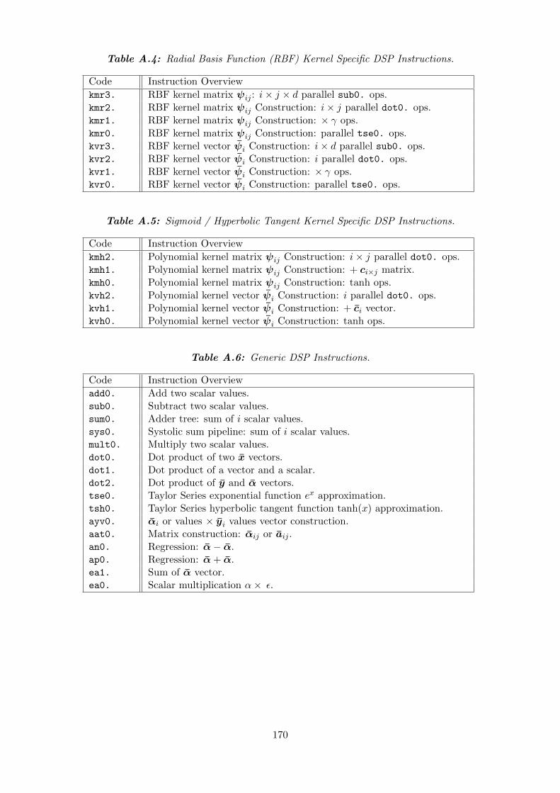
Table A.4: Radial Basis Function (RBF) Kernel Specific DSP Instructions.
Code Instruction Overview
kmr3. RBF kernel matrix ψij : i× j × d parallel sub0. ops.
kmr2. RBF kernel matrix ψij Construction: i× j parallel dot0. ops.
kmr1. RBF kernel matrix ψij Construction: × γ ops.
kmr0. RBF kernel matrix ψij Construction: parallel tse0. ops.
kvr3. RBF kernel vector ψi Construction: i× d parallel sub0. ops.kvr2. RBF kernel vector ψi Construction: i parallel dot0. ops.kvr1. RBF kernel vector ψi Construction: × γ ops.kvr0. RBF kernel vector ψi Construction: parallel tse0. ops.
Table A.5: Sigmoid / Hyperbolic Tangent Kernel Specific DSP Instructions.
Code Instruction Overview
kmh2. Polynomial kernel matrix ψij Construction: i× j parallel dot0. ops.
kmh1. Polynomial kernel matrix ψij Construction: + ci×j matrix.
kmh0. Polynomial kernel matrix ψij Construction: tanh ops.
kvh2. Polynomial kernel vector ψi Construction: i parallel dot0. ops.kvh1. Polynomial kernel vector ψi Construction: + ci vector.kvh0. Polynomial kernel vector ψi Construction: tanh ops.
Table A.6: Generic DSP Instructions.
Code Instruction Overview
add0. Add two scalar values.sub0. Subtract two scalar values.sum0. Adder tree: sum of i scalar values.sys0. Systolic sum pipeline: sum of i scalar values.mult0. Multiply two scalar values.dot0. Dot product of two x vectors.dot1. Dot product of a vector and a scalar.dot2. Dot product of y and α vectors.tse0. Taylor Series exponential function ex approximation.tsh0. Taylor Series hyperbolic tangent function tanh(x) approximation.ayv0. αi or values × yi values vector construction.aat0. Matrix construction: αij or aij .an0. Regression: α− α.ap0. Regression: α+ α.ea1. Sum of α vector.ea0. Scalar multiplication α× ε.
170
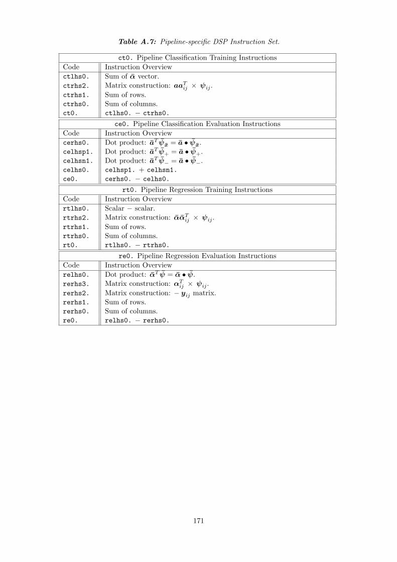
Table A.7: Pipeline-specific DSP Instruction Set.
ct0. Pipeline Classification Training Instructions
Code Instruction Overview
ctlhs0. Sum of α vector.
ctrhs2. Matrix construction: aaTij × ψij .
ctrhs1. Sum of rows.ctrhs0. Sum of columns.ct0. ctlhs0. − ctrhs0.
ce0. Pipeline Classification Evaluation Instructions
Code Instruction Overview
cerhs0. Dot product: aT ψx = a • ψx.celhsp1. Dot product: aT ψ+ = a • ψ+.celhsn1. Dot product: aT ψ− = a • ψ−.celhs0. celhsp1. + celhsn1.
ce0. cerhs0. − celhs0.
rt0. Pipeline Regression Training Instructions
Code Instruction Overview
rtlhs0. Scalar − scalar.
rtrhs2. Matrix construction: ααTij × ψij .
rtrhs1. Sum of rows.rtrhs0. Sum of columns.rt0. rtlhs0. − rtrhs0.
re0. Pipeline Regression Evaluation Instructions
Code Instruction Overview
relhs0. Dot product: αT ψ = α • ψ.
rerhs3. Matrix construction: αTij × ψij .
rerhs2. Matrix construction: − yij matrix.
rerhs1. Sum of rows.rerhs0. Sum of columns.re0. relhs0. − rerhs0.
171
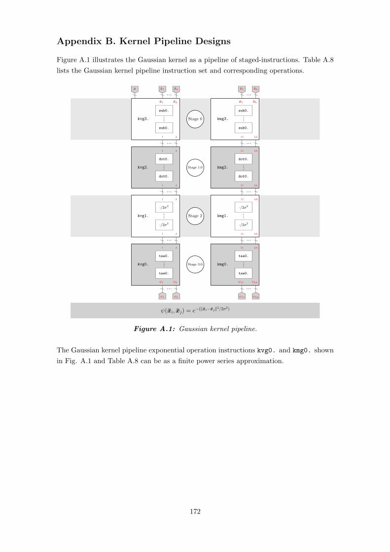
Appendix B. Kernel Pipeline Designs
Figure A.1 illustrates the Gaussian kernel as a pipeline of staged-instructions. Table A.8
lists the Gaussian kernel pipeline instruction set and corresponding operations.
kmg3.
x1 xk
sub0.
sub0.
Stage 0
Stage 1.0
Stage 2
Stage 3.0
kmg1.
x1 xk
dot0.
dot0.
kmg2.
kmg0.
ψ11 ψkk
tse0.
tse0.
11 kk
ψ11 ψkk
kvg3.
x1 xk
1 k
sub0.
sub0.
kvg1.
x1 xk
dot0.
dot0.
1 k
kvg2.
1 k
kvg0.
ψ1 ψk
tse0.
tse0.
1 k
1 k
1 k
ψ1 ψk
11 kk
11 kk
11 kk
11 kk
11 kk
x
·/2σ2
·/2σ2
·/2σ2
·/2σ2
ψ(xi, xj) = e−(‖xi−xj‖2/2σ2)
Figure A.1: Gaussian kernel pipeline.
The Gaussian kernel pipeline exponential operation instructions kvg0. and kmg0. shown
in Fig. A.1 and Table A.8 can be as a finite power series approximation.
172

Table A.8: Gaussian kernel pipeline instruction overview.
⇒
x1 − x
...xk − x
⇒
‖x1 − x‖2/2σ2
...‖xk − x‖2/2σ2
⇒
e−(‖x1−x‖2/2σ2)
...
e−(‖xk−x‖2/2σ2)
=
ψ1
...ψk
= ψ
kvg1.
kvg0.
ψ(xi, x)⇒ ψi×1 = ψ
kvg3.
⇒
x1 − x1 · · · x1 − xk
.... . .
...xk − x1 · · · xk − xk
⇒
‖x1 − x1‖2/2σ2 · · · ‖x1 − xk‖2/2σ2
.... . .
...‖xk − x1‖2/2σ2 · · · ‖xk − xk‖2/2σ2
kmg3.
kmg1.
ψ(xi, xj)⇒ ψi×j = ψ
kmg0. ⇒
e−(‖x1−x1‖2/2σ2) · · · e−(‖x1−xk‖2/2σ2)
.... . .
...
e−(‖xk−x1‖2/2σ2) · · · e−(‖xk−xk‖2/2σ2)
=
ψ11 · · · ψ1k
.... . .
...ψk1 · · · ψkk
= ψ
⇒
‖x1 − x‖2
...‖xk − x‖2
=
a1 · a1
...ak · ak
kvg2.
⇒
‖x1 − x1‖2 · · · ‖x1 − xk‖2
.... . .
...‖xk − x1‖2 · · · ‖xk − xk‖2
=
a1 · a1 · · · a1 · ak
.... . .
...ak · a1 · · · ak · ak
kmg2.
Mathematical OperationInstruction
Figure A.2 illustrates the Radial Basis Function (RBF) kernel as a pipeline of staged-
instructions. Table A.9 lists the Radial Basis Function (RBF) kernel pipeline instruction
set and corresponding operations.
173

kmr3.
x1 xk
sub0.
sub0.
Stage 0
Stage 1.0
Stage 2
Stage 3.0
kmr1.
x1 xk
dot0.
dot0.
kmr2.
kmr0.
ψ11 ψkk
tse0.
tse0.
11 kk
ψ11 ψkk
kvr3.
x1 xk
1 k
sub0.
sub0.
· γ
kvr1.
x1 xk
dot0.
dot0.
1 k
kvr2.
1 k
kvr0.
ψ1 ψk
tse0.
tse0.
1 k
1 k
1 k
ψ1 ψk
11 kk
11 kk
11 kk
11 kk
11 kk
ψ(xi, xj) = e−(γ‖xi−xj‖2)
· γ
· γ
· γ
x
Figure A.2: Radial Basis Function (RBF) kernel pipeline.
The Radial Basis Function kernel pipeline exponential operation instructions kvr0. and
kmr0. shown in Fig. A.2 and Table A.9 can be as a finite power series approximation.
174

Table A.9: Radial Basis Function (RBF) kernel pipeline instruction overview.
⇒
x1 − x
...xk − x
⇒
γ‖x1 − x‖2
...γ‖xk − x‖2
⇒
e−(γ‖x1−x‖2)
...
e−(γ‖xk−x‖2)
=
ψ1
...ψk
= ψ
kvg1.
kvg0.
ψ(xi, x)⇒ ψi×1 = ψ
kvg3.
⇒
x1 − x1 · · · x1 − xk
.... . .
...xk − x1 · · · xk − xk
⇒
γ‖x1 − x1‖2 · · · γ‖x1 − xk‖2
.... . .
...γ‖xk − x1‖2 · · · γ‖xk − xk‖2
kmg3.
kmg1.
ψ(xi, xj)⇒ ψi×j = ψ
kmg0. ⇒
e−(γ‖x1−x1‖2) · · · e−(γ‖x1−xk‖2)
.... . .
...
e−(γ‖xk−x1‖2) · · · e−(γ‖xk−xk‖2)
=
ψ11 · · · ψ1k
.... . .
...ψk1 · · · ψkk
= ψ
⇒
‖x1 − x‖2
...‖xk − x‖2
=
a1 · a1
...ak · ak
kvg2.
⇒
‖x1 − x1‖2 · · · ‖a1 − ak‖2
.... . .
...‖xk − x1‖2 · · · ‖xk − xk‖2
=
a1 · a1 · · · a1 · ak
.... . .
...ak · a1 · · · ak · ak
kmg2.
Mathematical OperationInstruction
Figure A.3 illustrates the Sigmoid / Hyperbolic Tangent kernel as a pipeline of staged-
instructions. Table A.10 lists the Sigmoid / Hyperbolic Tangent kernel pipeline instruction
set and corresponding operations.
The Sigmoid / Hyperbolic Tangent kernel pipeline hyperbolic-tangent operation instruc-
tions kvh0. and kmh0. shown in Fig. A.3 and Table A.10 can be as a finite Taylor series
approximation.
175

kmh2.
x1 xk
11 kk
kmh1.
+ c
+ c
dot0.
dot0.
Stage 0.0
Stage 1
Stage 2.0
ψ11 ψkk
kmh0.
x1 xk
ψ11 ψkk
kvh2.
x1 xk
1 k
kvh1.
+ c
+ c
dot0.
dot0.
ψ1 ψk
kvh0.
x1 xk
ψ1 ψk
1 k
1 k
1 k
11 kk
11 kk
11 kk
ψ(xi, xj) = tanh(xi • xj + c)
tanh(·)
tanh(·)
tanh(·)
tanh(·)
x
Figure A.3: Sigmoid / Hyperbolic Tangent Kernel Pipeline.
Table A.10: Sigmoid / Hyperbolic Tangent kernel pipeline instruction overview.
⇒
x1 · x
...xk · x
⇒
[x1 · x] + c...
[xk · x] + c
⇒
tanh([x1 · x] + c)...
tanh([xk · x] + c)
=
ψ1
...ψk
= ψ
kvh1.
kvh0.
ψ(xi, x)⇒ ψi×1 = ψ
kvh2.
⇒
x1 · x1 · · · x1 · xk
.... . .
...xk · x1 · · · xk · xk
⇒
[x1 · x1] + c · · · [x1 · xk] + c...
. . ....
[xk · x1] + c · · · [xk · xk] + c
⇒
tanh([x1 · x1] + c) · · · tanh([x1 · xk] + c)...
. . ....
tanh([xk · x1] + c) · · · tanh([xk · xk] + c)
=
ψ11 · · · ψ1k
.... . .
...ψk1 · · · ψkk
= ψ
kmh2.
kmh1.
kmh0.
ψ(xi, xj)⇒ ψi×j = ψ
Mathematical OperationInstruction
176

Appendix C. Implemented Pipeline Entities
Listing A.1 provides the VHDL Entity for dsp d2 k4 ct0. Classification Evaluation
Pipeline. Listing A.2 provides the VHDL Entity for dsp d2 k8 ct0. Classification Eval-
uation Pipeline. Listing A.3 provides the VHDL Entity for dsp d2 k16 ct0. Classifi-
cation Evaluation Pipeline. Listing A.4 provides the VHDL Entity for dsp d2 k32 ct0.
Classification Evaluation Pipeline.
Listing A.1: VHDL Entity: dsp d2 k4 ct0. Classification Evaluation Pipeline.� �1 -- dsp_d2_k4_ct0 Entity
2 ENTITY dsp_d2_k4_ct0 IS
3 GENERIC
4 (
5 CT0_D_C : NATURAL := 2;
6 CT0_K_C : NATURAL := 4;
7 CT0_ST_C : NATURAL := 9
8 );
9 PORT
10 (
11 -- Control io
12 clk : IN STD_LOGIC;
13 rst : IN STD_LOGIC;
14 en : IN STD_LOGIC;
15 valid : OUT STD_LOGIC;
16 -- Input Signals
17 xv : IN CT0_X_ARRAY;
18 a : IN CT0_A_TYPE;
19 y : IN CT0_Y_TYPE;
20 -- Output.
21 ct0 : OUT CT0_TYPE
22 );
23 END dsp_d2_k4_ct0;� �Listing A.2: VHDL Entity: dsp d2 k8 ct0. Classification Evaluation Pipeline.� �
1 -- dsp_d2_k8_ct0 Entity
2 ENTITY dsp_d2_k8_ct0 IS
3 GENERIC
4 (
5 CT0_D_C : NATURAL := 2;
6 CT0_K_C : NATURAL := 8;
7 CT0_ST_C : NATURAL := 11
8 );
9 PORT
10 (
11 -- Control io
12 clk : IN STD_LOGIC;
13 rst : IN STD_LOGIC;
14 en : IN STD_LOGIC;
15 valid : OUT STD_LOGIC;
16 -- Input Signals
17 xv : IN CT0_X_ARRAY;
18 a : IN CT0_A_TYPE;
19 y : IN CT0_Y_TYPE;
20 -- Output.
21 ct0 : OUT CT0_TYPE
22 );
23 END dsp_d2_k8_ct0;
177

� �Listing A.3: VHDL Entity: dsp d2 k16 ct0. Classification Evaluation Pipeline.� �
1 -- dsp_d2_k16_ct0 Entity
2 ENTITY dsp_d2_k16_ct0 IS
3 GENERIC
4 (
5 CT0_D_C : NATURAL := 2;
6 CT0_K_C : NATURAL := 16;
7 CT0_ST_C : NATURAL := 13
8 );
9 PORT
10 (
11 -- Control io
12 clk : IN STD_LOGIC;
13 rst : IN STD_LOGIC;
14 en : IN STD_LOGIC;
15 valid : OUT STD_LOGIC;
16 -- Input Signals
17 xv : IN CT0_X_ARRAY;
18 a : IN CT0_A_TYPE;
19 y : IN CT0_Y_TYPE;
20 -- Output.
21 ct0 : OUT CT0_TYPE
22 );
23 END dsp_d2_k16_ct0;� �Listing A.4: VHDL Entity: dsp d2 k32 ct0. Classification Evaluation Pipeline.� �
1 -- dsp_d2_k32_ct0 Entity
2 ENTITY dsp_d2_k32_ct0 IS
3 GENERIC
4 (
5 CT0_D_C : NATURAL := 2;
6 CT0_K_C : NATURAL := 32;
7 CT0_ST_C : NATURAL := 15
8 );
9 PORT
10 (
11 -- Control io
12 clk : IN STD_LOGIC;
13 rst : IN STD_LOGIC;
14 en : IN STD_LOGIC;
15 valid : OUT STD_LOGIC;
16 -- Input Signals
17 xv : IN CT0_X_ARRAY;
18 a : IN CT0_A_TYPE;
19 y : IN CT0_Y_TYPE;
20 -- Output.
21 ct0 : OUT CT0_TYPE
22 );
23 END dsp_d2_k32_ct0;� �Listing A.5 provides the VHDL Entity for dsp d4 k8 ct0. Classification Evaluation
Pipeline. Listing A.6 provides the VHDL Entity for dsp d4 k16 ct0. Classification
Evaluation Pipeline. Listing A.7 provides the VHDL Entity for dsp d4 k32 ct0. Classi-
fication Evaluation Pipeline.
178

Listing A.5: VHDL Entity: dsp d4 k8 ct0. Classification Evaluation Pipeline.� �1 -- dsp_d4_k8_ct0 Entity
2 ENTITY dsp_d4_k8_ct0 IS
3 GENERIC
4 (
5 CT0_D_C : NATURAL := 4;
6 CT0_K_C : NATURAL := 8;
7 CT0_ST_C : NATURAL := 11
8 );
9 PORT
10 (
11 -- Control io
12 clk : IN STD_LOGIC;
13 rst : IN STD_LOGIC;
14 en : IN STD_LOGIC;
15 valid : OUT STD_LOGIC;
16 -- Input Signals
17 xv : IN CT0_X_ARRAY;
18 a : IN CT0_A_TYPE;
19 y : IN CT0_Y_TYPE;
20 -- Output.
21 ct0 : OUT CT0_TYPE
22 );
23 END dsp_d4_k8_ct0;� �Listing A.6: VHDL Entity: dsp d4 k16 ct0. Classification Evaluation Pipeline.� �
1 -- dsp_d4_k16_ct0 Entity
2 ENTITY dsp_d4_k16_ct0 IS
3 GENERIC
4 (
5 CT0_D_C : NATURAL := 4;
6 CT0_K_C : NATURAL := 16;
7 CT0_ST_C : NATURAL := 13
8 );
9 PORT
10 (
11 -- Control io
12 clk : IN STD_LOGIC;
13 rst : IN STD_LOGIC;
14 en : IN STD_LOGIC;
15 valid : OUT STD_LOGIC;
16 -- Input Signals
17 xv : IN CT0_X_ARRAY;
18 a : IN CT0_A_TYPE;
19 y : IN CT0_Y_TYPE;
20 -- Output.
21 ct0 : OUT CT0_TYPE
22 );
23 END dsp_d4_k16_ct0;� �Listing A.7: VHDL Entity: dsp d4 k32 ct0. Classification Evaluation Pipeline.� �
1 -- dsp_d4_k32_ct0 Entity
2 ENTITY dsp_d4_k32_ct0 IS
3 GENERIC
4 (
5 CT0_D_C : NATURAL := 4;
6 CT0_K_C : NATURAL := 32;
179

7 CT0_ST_C : NATURAL := 15
8 );
9 PORT
10 (
11 -- Control io
12 clk : IN STD_LOGIC;
13 rst : IN STD_LOGIC;
14 en : IN STD_LOGIC;
15 valid : OUT STD_LOGIC;
16 -- Input Signals
17 xv : IN CT0_X_ARRAY;
18 a : IN CT0_A_TYPE;
19 y : IN CT0_Y_TYPE;
20 -- Output.
21 ct0 : OUT CT0_TYPE
22 );
23 END dsp_d4_k32_ct0;� �Listing A.8 provides the VHDL Entity for dsp d8 k16 ct0. Classification Evaluation
Pipeline. Listing A.9 provides the VHDL Entity for dsp d8 k32 ct0. Classification
Evaluation Pipeline.
Listing A.8: VHDL Entity: dsp d8 k16 ct0. Classification Evaluation Pipeline.� �1 -- dsp_d8_k16_ct0 Entity
2 ENTITY dsp_d8_k16_ct0 IS
3 GENERIC
4 (
5 CT0_D_C : NATURAL := 8;
6 CT0_K_C : NATURAL := 16;
7 CT0_ST_C : NATURAL := 14
8 );
9 PORT
10 (
11 -- Control io
12 clk : IN STD_LOGIC;
13 rst : IN STD_LOGIC;
14 en : IN STD_LOGIC;
15 valid : OUT STD_LOGIC;
16 -- Input Signals
17 xv : IN CT0_X_ARRAY;
18 a : IN CT0_A_TYPE;
19 y : IN CT0_Y_TYPE;
20 -- Output.
21 ct0 : OUT CT0_TYPE
22 );
23 END dsp_d8_k16_ct0;� �Listing A.9: VHDL Entity: dsp d8 k32 ct0. Classification Evaluation Pipeline.� �
1 -- dsp_d8_k32_ct0 Entity
2 ENTITY dsp_d8_k32_ct0 IS
3 GENERIC
4 (
5 CT0_D_C : NATURAL := 8;
6 CT0_K_C : NATURAL := 32;
7 CT0_ST_C : NATURAL := 15
8 );
9 PORT
10 (
180

11 -- Control io
12 clk : IN STD_LOGIC;
13 rst : IN STD_LOGIC;
14 en : IN STD_LOGIC;
15 valid : OUT STD_LOGIC;
16 -- Input Signals
17 xv : IN CT0_X_ARRAY;
18 a : IN CT0_A_TYPE;
19 y : IN CT0_Y_TYPE;
20 -- Output.
21 ct0 : OUT CT0_TYPE
22 );
23 END dsp_d8_k32_ct0;� �Listing A.10 provides the VHDL Entity for dsp d2 k4 ce0. Classification Evaluation
Pipeline. Listing A.11 provides the VHDL Entity for dsp d2 k8 ce0. Classification Eval-
uation Pipeline. Listing A.12 provides the VHDL Entity for dsp d2 k16 ce0. Classifica-
tion Evaluation Pipeline. Listing A.13 provides the VHDL Entity for dsp d2 k32 ce0.
Classification Evaluation Pipeline.
Listing A.10: VHDL Entity: dsp d2 k4 ce0. Classification Evaluation Pipeline.� �1 -- dsp_d2_k4_ce0 Entity
2 ENTITY dsp_d2_k4_ce0 IS
3 GENERIC
4 (
5 CE0_D_C : NATURAL := 2;
6 CE0_K_C : NATURAL := 4;
7 CE0_ST_C : NATURAL := 8
8 );
9 PORT
10 (
11 -- Ports go here
12 clk : IN STD_LOGIC;
13 rst : IN STD_LOGIC;
14 en : IN STD_LOGIC;
15 valid : OUT STD_LOGIC;
16 -- Input Signals
17 xv : IN CE0_X_ARRAY;
18 x : IN CE0_X_TYPE;
19 xp : IN CE0_X_TYPE;
20 xn : IN CE0_X_TYPE;
21 a : IN CE0_A_TYPE;
22 y : IN CE0_Y_TYPE;
23 -- Output.
24 ce0 : OUT CE0_TYPE
25 );
26 END dsp_d2_k4_ce0;� �Listing A.11: VHDL Entity: dsp d2 k8 ce0. Classification Evaluation Pipeline.� �
1 -- dsp_d2_k8_ce0 Entity
2 ENTITY dsp_d2_k8_ce0 IS
3 GENERIC
4 (
5 CE0_D_C : NATURAL := 2;
6 CE0_K_C : NATURAL := 8;
7 CE0_ST_C : NATURAL := 9
8 );
181

9 PORT
10 (
11 -- Ports go here
12 clk : IN STD_LOGIC;
13 rst : IN STD_LOGIC;
14 en : IN STD_LOGIC;
15 valid : OUT STD_LOGIC;
16 -- Input Signals
17 xv : IN CE0_X_ARRAY;
18 x : IN CE0_X_TYPE;
19 xp : IN CE0_X_TYPE;
20 xn : IN CE0_X_TYPE;
21 a : IN CE0_A_TYPE;
22 y : IN CE0_Y_TYPE;
23 -- Output.
24 ce0 : OUT CE0_TYPE
25 );
26 END dsp_d2_k8_ce0;� �Listing A.12: VHDL Entity: dsp d2 k16 ce0. Classification Evaluation Pipeline.� �
1 -- dsp_d2_k16_ce0 Entity
2 ENTITY dsp_d2_k16_ce0 IS
3 GENERIC
4 (
5 CE0_D_C : NATURAL := 2;
6 CE0_K_C : NATURAL := 16;
7 CE0_ST_C : NATURAL := 10
8 );
9 PORT
10 (
11 -- Ports go here
12 clk : IN STD_LOGIC;
13 rst : IN STD_LOGIC;
14 en : IN STD_LOGIC;
15 valid : OUT STD_LOGIC;
16 -- Input Signals
17 xv : IN CE0_X_ARRAY;
18 x : IN CE0_X_TYPE;
19 xp : IN CE0_X_TYPE;
20 xn : IN CE0_X_TYPE;
21 a : IN CE0_A_TYPE;
22 y : IN CE0_Y_TYPE;
23 -- Output
24 ce0 : OUT CE0_TYPE
25 );
26 END dsp_d2_k16_ce0;� �Listing A.13: VHDL Entity: dsp d2 k32 ce0. Classification Evaluation Pipeline.� �
1 -- dsp_d2_k32_ce0 Entity
2 ENTITY dsp_d2_k32_ce0 IS
3 GENERIC
4 (
5 CE0_D_C : NATURAL := 2;
6 CE0_K_C : NATURAL := 32;
7 CE0_ST_C : NATURAL := 11
8 );
9 PORT
10 (
182

11 -- Ports go here
12 clk : IN STD_LOGIC;
13 rst : IN STD_LOGIC;
14 en : IN STD_LOGIC;
15 valid : OUT STD_LOGIC;
16 -- Input Signals
17 xv : IN CE0_X_ARRAY;
18 x : IN CE0_X_TYPE;
19 xp : IN CE0_X_TYPE;
20 xn : IN CE0_X_TYPE;
21 a : IN CE0_A_TYPE;
22 y : IN CE0_Y_TYPE;
23 -- Output.
24 ce0 : OUT CE0_TYPE
25 );
26 END dsp_d2_k32_ce0;� �Listing A.14 provides the VHDL Entity for dsp d4 k8 ce0. Classification Evaluation
Pipeline. Listing A.15 provides the VHDL Entity for dsp d4 k16 ce0. Classification
Evaluation Pipeline. Listing A.16 provides the VHDL Entity for dsp d4 k32 ce0. Clas-
sification Evaluation Pipeline.
Listing A.14: VHDL Entity: dsp d4 k8 ce0. Classification Evaluation Pipeline.� �1 -- dsp_d4_k8_ce0 Entity
2 ENTITY dsp_d4_k8_ce0 IS
3 GENERIC
4 (
5 CE0_D_C : NATURAL := 4;
6 CE0_K_C : NATURAL := 8;
7 CE0_ST_C : NATURAL := 9
8 );
9 PORT
10 (
11 -- Ports go here
12 clk : IN STD_LOGIC;
13 rst : IN STD_LOGIC;
14 en : IN STD_LOGIC;
15 valid : OUT STD_LOGIC;
16 -- Input Signals
17 xv : IN CE0_X_ARRAY;
18 x : IN CE0_X_TYPE;
19 xp : IN CE0_X_TYPE;
20 xn : IN CE0_X_TYPE;
21 a : IN CE0_A_TYPE;
22 y : IN CE0_Y_TYPE;
23 -- Output.
24 ce0 : OUT CE0_TYPE
25 );
26 END dsp_d4_k8_ce0;� �Listing A.15: VHDL Entity: dsp d4 k16 ce0. Classification Evaluation Pipeline.� �
1 -- dsp_d4_k16_ce0 Entity
2 ENTITY dsp_d4_k16_ce0 IS
3 GENERIC
4 (
5 CE0_D_C : NATURAL := 4;
6 CE0_K_C : NATURAL := 16;
183

7 CE0_ST_C : NATURAL := 10
8 );
9 PORT
10 (
11 -- Ports go here
12 clk : IN STD_LOGIC;
13 rst : IN STD_LOGIC;
14 en : IN STD_LOGIC;
15 valid : OUT STD_LOGIC;
16 -- Input Signals
17 xv : IN CE0_X_ARRAY;
18 x : IN CE0_X_TYPE;
19 xp : IN CE0_X_TYPE;
20 xn : IN CE0_X_TYPE;
21 a : IN CE0_A_TYPE;
22 y : IN CE0_Y_TYPE;
23 -- Output.
24 ce0 : OUT CE0_TYPE
25 );
26 END dsp_d4_k16_ce0;� �Listing A.16: VHDL Entity: dsp d4 k32 ce0. Classification Evaluation Pipeline.� �
1 -- dsp_d4_k32_ce0 Entity
2 ENTITY dsp_d4_k32_ce0 IS
3 GENERIC
4 (
5 CE0_D_C : NATURAL := 4;
6 CE0_K_C : NATURAL := 32;
7 CE0_ST_C : NATURAL := 11
8 );
9 PORT
10 (
11 -- Ports go here
12 clk : IN STD_LOGIC;
13 rst : IN STD_LOGIC;
14 en : IN STD_LOGIC;
15 valid : OUT STD_LOGIC;
16 -- Input Signals
17 xv : IN CE0_X_ARRAY;
18 x : IN CE0_X_TYPE;
19 xp : IN CE0_X_TYPE;
20 xn : IN CE0_X_TYPE;
21 a : IN CE0_A_TYPE;
22 y : IN CE0_Y_TYPE;
23 -- Output.
24 ce0 : OUT CE0_TYPE
25 );
26 END dsp_d4_k32_ce0;� �Listing A.17 provides the VHDL Entity for dsp d8 k16 ce0. Classification Evaluation
Pipeline. Listing A.18 provides the VHDL Entity for dsp d8 k32 ce0. Classification
Evaluation Pipeline.
Listing A.17: VHDL Entity: dsp d8 k16 ce0. Classification Evaluation Pipeline.� �1 -- dsp_d8_k16_ce0 Entity
2 ENTITY dsp_d8_k16_ce0 IS
3 GENERIC
4 (
184
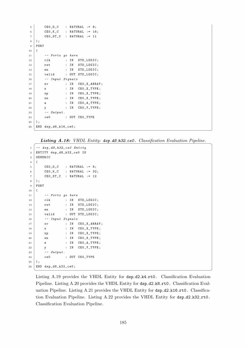
5 CE0_D_C : NATURAL := 8;
6 CE0_K_C : NATURAL := 16;
7 CE0_ST_C : NATURAL := 11
8 );
9 PORT
10 (
11 -- Ports go here
12 clk : IN STD_LOGIC;
13 rst : IN STD_LOGIC;
14 en : IN STD_LOGIC;
15 valid : OUT STD_LOGIC;
16 -- Input Signals
17 xv : IN CE0_X_ARRAY;
18 x : IN CE0_X_TYPE;
19 xp : IN CE0_X_TYPE;
20 xn : IN CE0_X_TYPE;
21 a : IN CE0_A_TYPE;
22 y : IN CE0_Y_TYPE;
23 -- Output.
24 ce0 : OUT CE0_TYPE
25 );
26 END dsp_d8_k16_ce0;� �Listing A.18: VHDL Entity: dsp d8 k32 ce0. Classification Evaluation Pipeline.� �
1 -- dsp_d8_k32_ce0 Entity
2 ENTITY dsp_d8_k32_ce0 IS
3 GENERIC
4 (
5 CE0_D_C : NATURAL := 8;
6 CE0_K_C : NATURAL := 32;
7 CE0_ST_C : NATURAL := 12
8 );
9 PORT
10 (
11 -- Ports go here
12 clk : IN STD_LOGIC;
13 rst : IN STD_LOGIC;
14 en : IN STD_LOGIC;
15 valid : OUT STD_LOGIC;
16 -- Input Signals
17 xv : IN CE0_X_ARRAY;
18 x : IN CE0_X_TYPE;
19 xp : IN CE0_X_TYPE;
20 xn : IN CE0_X_TYPE;
21 a : IN CE0_A_TYPE;
22 y : IN CE0_Y_TYPE;
23 -- Output.
24 ce0 : OUT CE0_TYPE
25 );
26 END dsp_d8_k32_ce0;� �Listing A.19 provides the VHDL Entity for dsp d2 k4 rt0. Classification Evaluation
Pipeline. Listing A.20 provides the VHDL Entity for dsp d2 k8 rt0. Classification Eval-
uation Pipeline. Listing A.21 provides the VHDL Entity for dsp d2 k16 rt0. Classifica-
tion Evaluation Pipeline. Listing A.22 provides the VHDL Entity for dsp d2 k32 rt0.
Classification Evaluation Pipeline.
185

Listing A.19: VHDL Entity: dsp d2 k4 rt0. Classification Evaluation Pipeline.� �1 -- dsp_d2_k4_rt0 Entity
2 ENTITY dsp_d2_k4_rt0 IS
3 GENERIC
4 (
5 RT0_D_C : NATURAL := 2;
6 RT0_K_C : NATURAL := 4;
7 RT0_ST_C : NATURAL := 10
8 );
9 PORT
10 (
11 -- Control io
12 clk : IN STD_LOGIC;
13 rst : IN STD_LOGIC;
14 en : IN STD_LOGIC;
15 valid : OUT STD_LOGIC;
16 -- Input Signals
17 xv : IN RT0_X_ARRAY;
18 ad : IN RT0_A_TYPE;
19 ac : IN RT0_A_TYPE;
20 y : IN RT0_Y_TYPE;
21 -- Output
22 rt0 : OUT RT0_TYPE
23 );
24 END dsp_d2_k4_rt0;� �Listing A.20: VHDL Entity: dsp d2 k8 rt0. Classification Evaluation Pipeline.� �
1 -- dsp_d2_k8_rt0 Entity
2 ENTITY dsp_d2_k8_rt0 IS
3 GENERIC
4 (
5 RT0_D_C : NATURAL := 2;
6 RT0_K_C : NATURAL := 8;
7 RT0_ST_C : NATURAL := 12
8 );
9 PORT
10 (
11 -- Control io
12 clk : IN STD_LOGIC;
13 rst : IN STD_LOGIC;
14 en : IN STD_LOGIC;
15 valid : OUT STD_LOGIC;
16 -- Input Signals
17 xv : IN RT0_X_ARRAY;
18 ad : IN RT0_A_TYPE;
19 ac : IN RT0_A_TYPE;
20 y : IN RT0_Y_TYPE;
21 -- Output
22 rt0 : OUT RT0_TYPE
23 );
24 END dsp_d2_k8_rt0;� �Listing A.21: VHDL Entity: dsp d2 k16 rt0. Classification Evaluation Pipeline.� �
1 -- dsp_d2_k16_rt0 Entity
2 ENTITY dsp_d2_k16_rt0 IS
3 GENERIC
4 (
186

5 RT0_D_C : NATURAL := 2;
6 RT0_K_C : NATURAL := 16;
7 RT0_ST_C : NATURAL := 14
8 );
9 PORT
10 (
11 -- Control io
12 clk : IN STD_LOGIC;
13 rst : IN STD_LOGIC;
14 en : IN STD_LOGIC;
15 valid : OUT STD_LOGIC;
16 -- Input Signals
17 xv : IN RT0_X_ARRAY;
18 ad : IN RT0_A_TYPE;
19 ac : IN RT0_A_TYPE;
20 y : IN RT0_Y_TYPE;
21 -- Output
22 rt0 : OUT RT0_TYPE
23 );
24 END dsp_d2_k16_rt0;� �Listing A.22: VHDL Entity: dsp d2 k32 rt0. Classification Evaluation Pipeline.� �
1 -- dsp_d2_k32_rt0 Entity
2 ENTITY dsp_d2_k32_rt0 IS
3 GENERIC
4 (
5 RT0_D_C : NATURAL := 2;
6 RT0_K_C : NATURAL := 32;
7 RT0_ST_C : NATURAL := 16
8 );
9 PORT
10 (
11 -- Control io
12 clk : IN STD_LOGIC;
13 rst : IN STD_LOGIC;
14 en : IN STD_LOGIC;
15 valid : OUT STD_LOGIC;
16 -- Input Signals
17 xv : IN RT0_X_ARRAY;
18 ad : IN RT0_A_TYPE;
19 ac : IN RT0_A_TYPE;
20 y : IN RT0_Y_TYPE;
21 -- Output.
22 rt0 : OUT RT0_TYPE
23 );
24 END dsp_d2_k32_rt0;� �Listing A.23 provides the VHDL Entity for dsp d4 k8 rt0. Classification Evaluation
Pipeline. Listing A.24 provides the VHDL Entity for dsp d4 k16 rt0. Classification
Evaluation Pipeline. Listing A.25 provides the VHDL Entity for dsp d4 k32 rt0. Clas-
sification Evaluation Pipeline.
Listing A.23: VHDL Entity: dsp d4 k8 rt0. Classification Evaluation Pipeline.� �1 -- dsp_d4_k8_rt0 Entity
2 ENTITY dsp_d4_k8_rt0 IS
3 GENERIC
4 (
187

5 RT0_D_C : NATURAL := 4;
6 RT0_K_C : NATURAL := 8;
7 RT0_ST_C : NATURAL := 12
8 );
9 PORT
10 (
11 -- Control io
12 clk : IN STD_LOGIC;
13 rst : IN STD_LOGIC;
14 en : IN STD_LOGIC;
15 valid : OUT STD_LOGIC;
16 -- Input Signals
17 xv : IN RT0_X_ARRAY;
18 ad : IN RT0_A_TYPE;
19 ac : IN RT0_A_TYPE;
20 y : IN RT0_Y_TYPE;
21 -- Output
22 rt0 : OUT RT0_TYPE
23 );
24 END dsp_d4_k8_rt0;� �Listing A.24: VHDL Entity: dsp d4 k16 rt0. Classification Evaluation Pipeline.� �
1 -- dsp_d4_k16_rt0 Entity
2 ENTITY dsp_d4_k16_rt0 IS
3 GENERIC
4 (
5 RT0_D_C : NATURAL := 4;
6 RT0_K_C : NATURAL := 16;
7 RT0_ST_C : NATURAL := 14
8 );
9 PORT
10 (
11 -- Control io
12 clk : IN STD_LOGIC;
13 rst : IN STD_LOGIC;
14 en : IN STD_LOGIC;
15 valid : OUT STD_LOGIC;
16 -- Input Signals
17 xv : IN RT0_X_ARRAY;
18 ad : IN RT0_A_TYPE;
19 ac : IN RT0_A_TYPE;
20 y : IN RT0_Y_TYPE;
21 -- Output
22 rt0 : OUT RT0_TYPE
23 );
24 END dsp_d4_k16_rt0;� �Listing A.25: VHDL Entity: dsp d4 k32 rt0. Classification Evaluation Pipeline.� �
1 -- dsp_d4_k32_rt0 Entity
2 ENTITY dsp_d4_k32_rt0 IS
3 GENERIC
4 (
5 RT0_D_C : NATURAL := 4;
6 RT0_K_C : NATURAL := 32;
7 RT0_ST_C : NATURAL := 16
8 );
9 PORT
10 (
188

11 -- Control io
12 clk : IN STD_LOGIC;
13 rst : IN STD_LOGIC;
14 en : IN STD_LOGIC;
15 valid : OUT STD_LOGIC;
16 -- Input Signals
17 xv : IN RT0_X_ARRAY;
18 ad : IN RT0_A_TYPE;
19 ac : IN RT0_A_TYPE;
20 y : IN RT0_Y_TYPE;
21 -- Output
22 rt0 : OUT RT0_TYPE
23 );
24 END dsp_d4_k32_rt0;� �Listing A.26 provides the VHDL Entity for dsp d8 k16 rt0. Classification Evaluation
Pipeline. Listing A.27 provides the VHDL Entity for dsp d8 k32 rt0. Classification
Evaluation Pipeline.
Listing A.26: VHDL Entity: dsp d8 k16 rt0. Classification Evaluation Pipeline.� �1 -- dsp_d8_k16_rt0 Entity
2 ENTITY dsp_d8_k16_rt0 IS
3 GENERIC
4 (
5 RT0_D_C : NATURAL := 8;
6 RT0_K_C : NATURAL := 16;
7 RT0_ST_C : NATURAL := 15
8 );
9 PORT
10 (
11 -- Control io
12 clk : IN STD_LOGIC;
13 rst : IN STD_LOGIC;
14 en : IN STD_LOGIC;
15 valid : OUT STD_LOGIC;
16 -- Input Signals
17 xv : IN RT0_X_ARRAY;
18 ad : IN RT0_A_TYPE;
19 ac : IN RT0_A_TYPE;
20 y : IN RT0_Y_TYPE;
21 -- Output
22 rt0 : OUT RT0_TYPE
23 );
24 END dsp_d8_k16_rt0;� �Listing A.27: VHDL Entity: dsp d8 k32 rt0. Classification Evaluation Pipeline.� �
1 -- dsp_d8_k32_rt0 Entity
2 ENTITY dsp_d8_k32_rt0 IS
3 GENERIC
4 (
5 RT0_D_C : NATURAL := 8;
6 RT0_K_C : NATURAL := 32;
7 RT0_ST_C : NATURAL := 17
8 );
9 PORT
10 (
11 -- Control io
12 clk : IN STD_LOGIC;
189

13 rst : IN STD_LOGIC;
14 en : IN STD_LOGIC;
15 valid : OUT STD_LOGIC;
16 -- Input Signals
17 xv : IN RT0_X_ARRAY;
18 ad : IN RT0_A_TYPE;
19 ac : IN RT0_A_TYPE;
20 y : IN RT0_Y_TYPE;
21 -- Output
22 rt0 : OUT RT0_TYPE
23 );
24 END dsp_d8_k32_rt0;� �Listing A.28 provides the VHDL Entity for dsp d2 k4 re0. Classification Evaluation
Pipeline. Listing A.29 provides the VHDL Entity for dsp d2 k8 re0. Classification Eval-
uation Pipeline. Listing A.30 provides the VHDL Entity for dsp d2 k16 re0. Classifica-
tion Evaluation Pipeline. Listing A.31 provides the VHDL Entity for dsp d2 k32 re0.
Classification Evaluation Pipeline.
Listing A.28: VHDL Entity: dsp d2 k4 re0. Classification Evaluation Pipeline.� �1 -- dsp_d2_k4_re0 Entity
2 ENTITY dsp_d2_k4_re0 IS
3 GENERIC
4 (
5 RE0_D_C : NATURAL := 2;
6 RE0_K_C : NATURAL := 4;
7 RE0_ST_C : NATURAL := 10
8 );
9 PORT
10 (
11 -- Control io
12 clk : IN STD_LOGIC;
13 rst : IN STD_LOGIC;
14 en : IN STD_LOGIC;
15 valid : OUT STD_LOGIC;
16 -- Input Signals
17 xv : IN RE0_X_ARRAY;
18 x : IN RE0_X_TYPE;
19 ad : IN RE0_A_TYPE;
20 ac : IN RE0_A_TYPE;
21 y : IN RE0_Y_TYPE;
22 -- Output.
23 re0 : OUT RE0_TYPE
24 );
25 END dsp_d2_k4_re0;� �Listing A.29: VHDL Entity: dsp d2 k8 re0. Classification Evaluation Pipeline.� �
1 -- dsp_d2_k8_re0 Entity
2 ENTITY dsp_d2_k8_re0 IS
3 GENERIC
4 (
5 RE0_D_C : NATURAL := 2;
6 RE0_K_C : NATURAL := 8;
7 RE0_ST_C : NATURAL := 12
8 );
9 PORT
10 (
190

11 -- Control io
12 clk : IN STD_LOGIC;
13 rst : IN STD_LOGIC;
14 en : IN STD_LOGIC;
15 valid : OUT STD_LOGIC;
16 -- Input Signals
17 xv : IN RE0_X_ARRAY;
18 x : IN RE0_X_TYPE;
19 ad : IN RE0_A_TYPE;
20 ac : IN RE0_A_TYPE;
21 y : IN RE0_Y_TYPE;
22 -- Output.
23 re0 : OUT RE0_TYPE
24 );
25 END dsp_d2_k8_re0;� �Listing A.30: VHDL Entity: dsp d2 k16 re0. Classification Evaluation Pipeline.� �
1 -- dsp_d2_k16_re0 Entity
2 ENTITY dsp_d2_k16_re0 IS
3 GENERIC
4 (
5 RE0_D_C : NATURAL := 2;
6 RE0_K_C : NATURAL := 16;
7 RE0_ST_C : NATURAL := 14
8 );
9 PORT
10 (
11 -- Control io
12 clk : IN STD_LOGIC;
13 rst : IN STD_LOGIC;
14 en : IN STD_LOGIC;
15 valid : OUT STD_LOGIC;
16 -- Input Signals
17 xv : IN RE0_X_ARRAY;
18 x : IN RE0_X_TYPE;
19 ad : IN RE0_A_TYPE;
20 ac : IN RE0_A_TYPE;
21 y : IN RE0_Y_TYPE;
22 -- Output.
23 re0 : OUT RE0_TYPE
24 );
25 END dsp_d2_k16_re0;� �Listing A.31: VHDL Entity: dsp d2 k32 re0. Classification Evaluation Pipeline.� �
1 -- dsp_d2_k32_re0 Entity
2 ENTITY dsp_d2_k32_re0 IS
3 GENERIC
4 (
5 RE0_D_C : NATURAL := 2;
6 RE0_K_C : NATURAL := 32;
7 RE0_ST_C : NATURAL := 16
8 );
9 PORT
10 (
11 -- Control io
12 clk : IN STD_LOGIC;
13 rst : IN STD_LOGIC;
14 en : IN STD_LOGIC;
191

15 valid : OUT STD_LOGIC;
16 -- Input Signals
17 xv : IN RE0_X_ARRAY;
18 x : IN RE0_X_TYPE;
19 ad : IN RE0_A_TYPE;
20 ac : IN RE0_A_TYPE;
21 y : IN RE0_Y_TYPE;
22 -- Output
23 re0 : OUT RE0_TYPE
24 );
25 END dsp_d2_k32_re0;� �Listing A.32 provides the VHDL Entity for dsp d4 k8 re0. Classification Evaluation
Pipeline. Listing A.33 provides the VHDL Entity for dsp d4 k16 re0. Classification
Evaluation Pipeline. Listing A.34 provides the VHDL Entity for dsp d4 k32 re0. Clas-
sification Evaluation Pipeline.
Listing A.32: VHDL Entity: dsp d4 k8 re0. Classification Evaluation Pipeline.� �1 -- dsp_d4_k8_re0 Entity
2 ENTITY dsp_d4_k8_re0 IS
3 GENERIC
4 (
5 RE0_D_C : NATURAL := 4;
6 RE0_K_C : NATURAL := 8;
7 RE0_ST_C : NATURAL := 12
8 );
9 PORT
10 (
11 -- Control io
12 clk : IN STD_LOGIC;
13 rst : IN STD_LOGIC;
14 en : IN STD_LOGIC;
15 valid : OUT STD_LOGIC;
16 -- Input Signals
17 xv : IN RE0_X_ARRAY;
18 x : IN RE0_X_TYPE;
19 ad : IN RE0_A_TYPE;
20 ac : IN RE0_A_TYPE;
21 y : IN RE0_Y_TYPE;
22 -- Output.
23 re0 : OUT RE0_TYPE
24 );
25 END dsp_d4_k8_re0;� �Listing A.33: VHDL Entity: dsp d4 k16 re0. Classification Evaluation Pipeline.� �
1 -- dsp_d4_k16_re0 Entity
2 ENTITY dsp_d4_k16_re0 IS
3 GENERIC
4 (
5 RE0_D_C : NATURAL := 4;
6 RE0_K_C : NATURAL := 16;
7 RE0_ST_C : NATURAL := 14
8 );
9 PORT
10 (
11 -- Control io
12 clk : IN STD_LOGIC;
192

13 rst : IN STD_LOGIC;
14 en : IN STD_LOGIC;
15 valid : OUT STD_LOGIC;
16 -- Input Signals
17 xv : IN RE0_X_ARRAY;
18 x : IN RE0_X_TYPE;
19 ad : IN RE0_A_TYPE;
20 ac : IN RE0_A_TYPE;
21 y : IN RE0_Y_TYPE;
22 -- Output.
23 re0 : OUT RE0_TYPE
24 );
25 END dsp_d4_k16_re0;� �Listing A.34: VHDL Entity: dsp d4 k32 re0. Classification Evaluation Pipeline.� �
1 -- dsp_d4_k32_re0 Entity
2 ENTITY dsp_d4_k32_re0 IS
3 GENERIC
4 (
5 RE0_D_C : NATURAL := 4;
6 RE0_K_C : NATURAL := 32;
7 RE0_ST_C : NATURAL := 16
8 );
9 PORT
10 (
11 -- Control io
12 clk : IN STD_LOGIC;
13 rst : IN STD_LOGIC;
14 en : IN STD_LOGIC;
15 valid : OUT STD_LOGIC;
16 -- Input Signals
17 xv : IN RE0_X_ARRAY;
18 x : IN RE0_X_TYPE;
19 ad : IN RE0_A_TYPE;
20 ac : IN RE0_A_TYPE;
21 y : IN RE0_Y_TYPE;
22 -- Output.
23 re0 : OUT RE0_TYPE
24 );
25 END dsp_d4_k32_re0;� �Listing A.35 provides the VHDL Entity for dsp d8 k16 re0. Classification Evaluation
Pipeline. Listing A.36 provides the VHDL Entity for dsp d8 k32 re0. Classification
Evaluation Pipeline.
Listing A.35: VHDL Entity: dsp d8 k16 re0. Classification Evaluation Pipeline.� �1 -- dsp_d8_k16_re0 Entity
2 ENTITY dsp_d8_k16_re0 IS
3 GENERIC
4 (
5 RE0_D_C : NATURAL := 8;
6 RE0_K_C : NATURAL := 16;
7 RE0_ST_C : NATURAL := 15
8 );
9 PORT
10 (
11 -- Control io
12 clk : IN STD_LOGIC;
193

13 rst : IN STD_LOGIC;
14 en : IN STD_LOGIC;
15 valid : OUT STD_LOGIC;
16 -- Input Signals
17 xv : IN RE0_X_ARRAY;
18 x : IN RE0_X_TYPE;
19 ad : IN RE0_A_TYPE;
20 ac : IN RE0_A_TYPE;
21 y : IN RE0_Y_TYPE;
22 -- Output.
23 re0 : OUT RE0_TYPE
24 );
25 END dsp_d8_k16_re0;� �Listing A.36: VHDL Entity: dsp d8 k32 re0. Classification Evaluation Pipeline.� �
1 -- dsp_d8_k32_re0 Entity
2 ENTITY dsp_d8_k32_re0 IS
3 GENERIC
4 (
5 RE0_D_C : NATURAL := 8;
6 RE0_K_C : NATURAL := 32;
7 RE0_ST_C : NATURAL := 17
8 );
9 PORT
10 (
11 -- Control io
12 clk : IN STD_LOGIC;
13 rst : IN STD_LOGIC;
14 en : IN STD_LOGIC;
15 valid : OUT STD_LOGIC;
16 -- Input Signals
17 xv : IN RE0_X_ARRAY;
18 x : IN RE0_X_TYPE;
19 ad : IN RE0_A_TYPE;
20 ac : IN RE0_A_TYPE;
21 y : IN RE0_Y_TYPE;
22 -- Output.
23 re0 : OUT RE0_TYPE
24 );
25 END dsp_d8_k32_re0;� �
194

References
[1] M. Al Rabieah and C. Bouganis, “Fpga based nonlinear support vector machine
training using an ensemble learning,” in Proc. of the 25th International Conference
on Field Programmable Logic and Applications (FPL), 09 2015, pp. 1–4.
[2] S. Afifi, H. GholamHosseini, and R. Sinha, Hardware Acceleration of
SVM-Based Classifier for Melanoma Images, F. Huang and A. Sugimoto,
Eds. Cham: Springer International Publishing, 2016. [Online]. Available:
https://doi.org/10.1007/978-3-319-30285-0 19
[3] S. Afifi, H. Gholamhosseini, and R. Sinha, “A low-cost fpga-based svm classifier for
melanoma detection,” in IEEE-EMBS Conference on Biomedical Engineering and
Sciences, L. Khuan, Ed. Kuala Lumpur, Malaysia, Dec 2016.
[4] B. E. Boser, I. Guyon, and V. Vapnik, “A training algorithm for optimal mar-
gin classifiers,” in Proc. of the 5th Annual Workshop on Computational Learning
Theory, Pittsburgh, PA, July 1992, pp. 144–152.
[5] F. Rosenblatt, “The perceptron: A probabilistic model for information storage and
organization in the brain,” Psychological Review, vol. 65, no. 6, pp. 386–408, 1958.
[6] G. E. Moore, “Cramming more components onto integrated circuits,” Electronics
Magazine, vol. 38, no. 8, pp. 114–117, April 1965.
[7] R. Kurzweil, The Age of Intelligent Machines. Cambridge, MA: The MIT Press,
1990.
[8] R. Kurzweil, The Age of Spiritual Machines: When Computers Exceed Human In-
telligence, 1st ed. New York, NY: Penguin USA, 1999.
[9] R. Kurzweil, The Singularity Is Near: When Humans Transcend Biology, 1st ed.
New York, NY: Viking, 2005.
[10] J. S. Kilby, “Miniaturised electronic circuits,” U.S. Patent 3 138 743, June 23, 1964.
[11] R. N. Noyce, “Semiconductor device-and-lead structure,” U.S. Patent 2 981 877,
April 25, 1961.
[12] (2012) IEEE Global History Network Milestones: First semiconductor in-
tegrated circuit (IC), 1958. [Online]. Available: http://ethw.org/Milestones:
First Semiconductor Integrated Circuit (IC), 1958
195

[13] S. Haykin, Neural Networks: A Comprehensive Foundation, 2nd ed. Upper Saddle
River, NJ: Prentice-Hall, Inc., 1998.
[14] M. Minsky and S. Papert, Perceptrons: An Introduction to Computational Geome-
try. Cambridge, MA: The MIT Press, 1969.
[15] H. P. Newquist, The Brain Makers, 1st ed. Santa Barbara, CA: Editors and
Engineers, Limited, 1994.
[16] I. Stewart, Does God Play Dice? The New Mathematics of Chaos, 2nd ed. Malden,
MA: Blackwell Publishing, 2002.
[17] J. Gleick, Chaos: Making a New Science, 2nd ed. New York, NY: Penguin Books,
2008.
[18] E. N. Lorenz, “Deterministic nonperiodic flow,” Journal of Atmospheric Sciences,
vol. 20, no. 2, pp. 130–148, 1963.
[19] B. B. Mandelbrot, The Fractal Geometry of Nature, 1st ed. New York, NY: Henry
Holt and Company, 1982.
[20] D. Hebb, The Organization of Behavior. New York, NY: Wiley & Sons, 1949.
[21] T. D. Sanger, “Optimal unsupervised learning in a single-layer linear feedforward
neural network,” Neural Netw., vol. 2, pp. 459–473, 1989.
[22] J. J. Hopfield and D. W. Tank, “Neural computation of decisions in optimization
problems,” Biological Cybernetics, vol. 52, no. 3, pp. 141–152, July 1985.
[23] D. E. Rumelhart, G. E. Hinton, and R. J. Williams, “Learning internal representa-
tions by error propagation,” in Parallel Distributed Processing: Explorations in the
Microstructure of Cognition; Foundations, D. E. Rumelhart, J. L. McClelland, and
the PDP Research Group, Eds. Cambridge, MA: The MIT Press, 1986, vol. 1.
[24] R. H. Freeman, “Configurable electrical circuit having configurable logic elements
and configurable interconnects,” U.S. Patent 4 870 302, September 26, 1989.
[25] C. Cortes and V. N. Vapnik, “Support-vector networks,” Machine Learning, vol. 20,
pp. 273–297, September 1995.
[26] V. N. Vapnik, The Nature of Statistical Learning Theory, 1st ed. New York, NY:
Springer-Verlag, 1995.
[27] V. N. Vapnik, Statistical Learning Theory, 1st ed. New York, NY: John Wiley &
Sons, Inc., 1998.
[28] V. N. Vapnik, “An overview of statistical learning theory,” IEEE Trans. Neural
Netw., vol. 10, no. 5, pp. 988–999, September 1999.
196

[29] R. K. Rajkumar, “Pipeline defect prediction using support vector machine,” Ph.D.
dissertation, Dept. of Elect. and Electron. Eng., Univ. of Nottingham, Kuala
Lumpur, Malaysia, 2011.
[30] D. Poole, Linear Algebra: A Modern Introduction, 2nd ed. Belmont, CA: Thomson
Brooks/Cole, 2006.
[31] L. Hamel, Knowledge Discovery with Support Vector Machines, 1st ed. New York,
NY: John Wiley & Sons, Inc., 2009.
[32] R. K. Sundaram, A First Course in Optimization Theory, 1st ed. Cambridge, UK:
Cambridge University Press, 1996.
[33] D. S. G. Pollock, A Handbook of Time Series Analysis, Signal Processing and Dy-
namics, 1st ed. San Diego, CA: Academic Press, 1999.
[34] K. Ogata, Modern Control Engineering, 4th ed. Upper Saddle River, NJ: Prentice-
Hall, Inc., 2002.
[35] R. H. Shumway and D. S. Stoffer, Time Series Analysis and Its Applications, 3rd ed.
New York, NY: Springer, 2011.
[36] D. G. Manolakis, V. K. Ingle, and S. M. Kogon, Statistical and Adaptive Signal
Processing: Spectral Estimation, Signal Modelling, Adaptive Filtering, and Array
Processing, 1st ed. Norwood, MA: Artech House, Inc., 2005.
[37] A. Cichocki and R. Unbehauen, Neural Networks for Optimization and Signal Pro-
cessing, 1st ed. New York, NY: John Wiley & Sons, Inc., 1993.
[38] V. N. Vapnik and A. Y. Chervonenkis, “On the uniform convergence of relative fre-
quencies of events to their probabilities,” Theory of Probability and its Applications,
vol. 16, no. 2, pp. 264–280, 1971.
[39] V. N. Vapnik, Estimation of Dependences Based on Empirical Data: Springer Series
in Statistics, 1st ed. Secaucus, NJ: Springer-Verlag New York, Inc., 1982.
[40] J. C. Platt, “Fast training of support vector machines using sequential minimal
optimization,” in Advances in Kernel Methods, B. Scholkopf, C. J. C. Burges, and
A. J. Smola, Eds. Cambridge, MA: The MIT Press, 1999, pp. 185–208.
[41] E. Osuna, R. Freund, and F. Girosi, “An improved training algorithm for support
vector machines,” in Proceedings of the 1997 IEEE Workshop on Neural Networks
for Signal Processing, Amelia Island, FL, September 1997, pp. 276–285.
[42] L. S. Lasdon, A. D. Waren, A. Jain, and M. Ratner, “Design and testing of a
generalized reduced gradient code for nonlinear programming,” ACM Transactions
on Mathematical Software (TOMS), vol. 4, no. 1, pp. 34–50, March 1978.
197
[43] S. Smith and L. S. Lasdon, “Solving large sparse nonlinear programs using GRG,”
INFORMS Journal on Computing, vol. 4, no. 1, pp. 2–15, February 1992.
[44] M. Jaggi, “Revisiting Frank-Wolfe: Projection-free sparse convex optimization,” in
Proceedings of the 30th International Conference on Machine Learning (ICML-13),
S. Dasgupta and D. Mcallester, Eds., vol. 28, no. 1, Atlanta, GA, June 2013, pp.
427–435.
[45] E. G. Gilbert, “An iterative procedure for computing the minimum of a quadratic
form on a convex set,” SIAM J. Control, vol. 4, no. 1, pp. 61–80, 1966.
[46] L. Chang, H. Qiao, A. Wan, and J. Keane, “An improved Gilbert algorithm with
rapid convergence,” in Proc. of the 2006 IEEE/RSJ Int. Conf. on Intelligent Robots
and Systems, Beijing, China, October 2006, pp. 3861–3866.
[47] J. A. Hartigan, Clustering Algorithms, 1st ed. New York, NY: John Wiley & Sons,
Inc., 1975.
[48] J. A. Hartigan and M. A. Wong, “Algorithm AS 136: A k-means clustering al-
gorithm,” Journal of the Royal Statistical Society. Series C (Applied Statistics),
vol. 28, no. 1, pp. 100–108, 1979.
[49] D. Anguita, A. Boni, and S. Ridella, “SVM learning with fixed-point math,” in
Proc. of the IEEE Int. Joint Conf. on Neural Netw. (IJCNN), Portland, OR, July
2003, pp. 2072–2076.
[50] D. Anguita, A. Boni, and S. Ridella, “A digital architecture for support vector
machines: Theory, algorithm, and FPGA implementation,” IEEE Trans. Neural
Netw., vol. 14, no. 5, pp. 993–1009, September 2003.
[51] S. Kim, S. Lee, K. Min, and K. Cho, “Design of support vector machine circuit
for real-time classification,” in Proc. of the IEEE Int. Symp. on Integrated Circuits,
2011 (ISIC 2011), Singapore, Singapore, December 2011, pp. 384–387.
[52] D. Mahmoodi, A. Soleimani, H. Khosravi, and M. Taghizadeh, “FPGA simulation
of linear and nonlinear support vector machine,” Journal of Software Engineering
and Applications, vol. 5, no. 4, pp. 320–328, 2011.
[53] K. Irick, M. DeBole, V. Narayanan, and A. Gayasen, “A hardware efficient support
vector machine architecture for FPGA,” in Proc. of the 16th IEEE Int. Symp. on
Field-Programmable Custom Computing Machines, 2008 (FCCM 2008), Palo Alto,
CA, April 2008, pp. 304–305.
[54] M. Ruiz-Llata, G. Guarnizo, and M. Yebenes-Calvino, “FPGA implementation of a
support vector machine for classification and regression,” in Proc. of the IEEE Int.
Joint Conf. on Neural Netw. (IJCNN), Barcelona, Spain, July 2010, pp. 477–481.
198

[55] J. G. Filho, M. Raffo, M. Strum, and W. J. Chau, “A general-purpose dynamically
reconfigurable SVM,” in Proc. of the IEEE VI Southern Programmable Logic Conf.
(SPL), Ipojuca, Brazil, March 2010, pp. 107–112.
[56] R. A. Patil, G. Gupta, V. Sahula, and A. S. Mandal, “Power aware hardware
prototyping of multiclass SVM classifier through reconfiguration,” in Proc. of the
IEEE 2012 25th Int. Conf. on VLSI Design (VLSID), Hyderabad, India, January
2012, pp. 62–67.
[57] M. E. Mavroforakis, M. Sdralis, and S. Theodoridis, “A novel SVM geometric al-
gorithm based on reduced convex hulls,” in Proc. of the 18th IEEE Int. Conf. on
Pattern Recognition (ICPR), Hong Kong, China, August 2006, pp. 564–568.
[58] S. Martin, “Training support vector machines using Gilbert’s algorithm,” in Proc.
of the 5th IEEE Int. Conf. on Data Mining (ICDM), Houston, TX, November 2005,
pp. 306–313.
[59] M. Papadonikolakis and C. Bouganis, “Efficient FPGA mapping of Gilbert’s al-
gorithm for SVM training on large-scale classification problems,” in Proc. of the
IEEE Int. Conf. on Field Programmable Logic and Applications (FPL), Heidelberg,
Germany, September 2008, pp. 385–390.
[60] M. Papadonikolakis and C. Bouganis, “A scalable FPGA architecture for non-linear
SVM training,” in Proc. of the IEEE Int. Conf. on Field-Programmable Technology
(FPT), Taipei, Taiwan, December 2008, pp. 337–340.
[61] M. Papadonikolakis, C. Bouganis, and G. Constantinides, “Performance compari-
son of GPU and FPGA architectures for the SVM training problem,” in Proc. of
the IEEE Int. Conf. on Field-Programmable Technology (FPT), Sydney, Australia,
December 2009, pp. 388–391.
[62] Z. B. Liu, J. G. Liu, and Z. Chen, “A generalized Gilbert’s algorithm for approx-
imating general SVM classifiers,” Neurocomputing, vol. 73, no. 1-3, pp. 219–224,
December 2009.
[63] M. Papadonikolakis and C. Bouganis, “A heterogeneous FPGA architecture for sup-
port vector machine training,” in Proc. of the IEEE Symp. on Field-Programmable
Custom Computing Machines, Charlotte, NC, May 2010, pp. 211–214.
[64] M. Papadonikolakis and C. Bouganis, “A novel FPGA-based SVM classifier,” in
Proc. of IEEE Int. Conf. on Field-Programmable Technology (FPT), Beijing, China,
December 2010, pp. 283–286.
[65] M. Papadonikolakis and C. Bouganis, “Novel cascade FPGA accelerator for support
vector machines classification,” IEEE Trans. Neural Netw. and Learning Systems,
vol. 23, no. 75, pp. 1040–1052, July 2012.
199

[66] C. Maxfield, The Design Warrior’s Guide to FPGAs, 1st ed. Orlando, FL: Aca-
demic Press, Inc., 2004.
[67] S. Brown and Z. Vranesic, Fundamentals of Digital Logic with VHDL Design, 3rd ed.
New York, NY: McGraw-Hill, Inc., 2008.
[68] R. Woods, J. Mcallister, R. Turner, Y. Yi, and G. Lightbody, FPGA-based Imple-
mentation of Signal Processing Systems, 1st ed. Chichester, UK: John Wiley &
Sons, Inc., 2008.
[69] “Accelerating DSP designs with the total 28-nm DSP portfolio,” White Paper,
Altera Corporation, April 2011.
[70] H. T. Kung and C. E. Leiserson, “Systolic arrays (for VLSI),” in SIAM Sparse
Matrix Proceedings 1978, I. S. Duff and G. W. Stewart, Eds. Philadelphia, PA:
SIAM Press, 1979, pp. 256–282.
[71] IEEE ASSP Magazine, VLSI Array Processors, vol. 2, no. 3, July 1985.
[72] S. Y. Kung, VLSI Array Processors, 1st ed. Englewood Cliffs, NJ: Prentice Hall,
1988.
[73] S. Y. Kung, “VLSI array processors: Designs and applications,” in Proc. of the
IEEE Int. Symp. on Circuits and Systems, 1988, vol. 1, Espoo, Finland, June 1988,
pp. 313–320.
[74] G. M. Amdahl, “Validity of the single processor approach to achieving large scale
computing capabilities,” in Proc. of the American Federation of Information Pro-
cessing Societies (AFIPS) Spring Joint Computer Conf., vol. 30. Atlantic City,
N.J.: AFIPS Press, Reston, Va., April 1967, pp. 483–485.
[75] G. Goslin, “Using xilinx FPGAs to design custom digital signal processing devices,”
in Proc. of the 1995 DSPX Technical Program Conference and Exhibition, San Jose,
CA, January 1995, pp. 595–604.
[76] J. C. Sprott, Chaos and Time-series Analysis, 1st ed. Oxford, UK: Oxford Uni-
versity Press, 2003.
[77] T. Kapitaniak and S. R. Bishop, The Illustrated Dictionary of Nonlinear Dynamics
and Chaos, 1st ed. New York, NY: John Wiley & Sons, Inc., 1999.
[78] L. Glass and M. C. Mackey, From Clocks to Chaos: The Rhythms of Life, 1st ed.
Princeton, NJ: Princeton University Press, 1988.
[79] D. J. Albers and J. C. Sprott, “Routes to chaos in neural networks with random
weights,” International Journal of Bifurcation and Chaos, vol. 8, no. 7, pp. 1463–
1478, May 1998.
200

[80] F. Takens, “Detecting strange attractors in turbulence,” in Dynamical Systems and
Turbulence, ser. Lecture Notes in Mathematics, D. A. Rand and L. S. Young, Eds.
Berlin, Germany: Springer-Verlag, 1981, vol. 898, pp. 366–381.
[81] H. D. I. Abarbanel, Analysis of Observed Chaotic Data, 1st ed. New York, NY:
Springer-Verlag, 1996.
[82] C. E. Shannon and W. Weaver, The Mathematical Theory of Communication,
2nd ed. Champaign, IL: University of Illinios Press, 1963.
[83] A. M. Fraser and H. L. Swinney, “Independent coordinates for strange attractors
from mutual information,” Physical Review A, vol. 33, no. 2, pp. 1134–1140, Febru-
ary 1986.
[84] A. M. Fraser, “Information and entropy in strange attractors,” IEEE Trans. on Inf.
Theory, vol. 35, no. 2, pp. 245–262, March 1989.
[85] M. B. Kennel, R. Brown, and H. D. I. Abarbanel, “Determining embedding di-
mension for phase-space reconstruction using a geometrical construction,” Physical
Review A, vol. 45, no. 6, pp. 3403–3411, March 1992.
[86] P. B. A. Phear, R. K. Rajkumar, and D. Isa, “Efficient non-iterative fixed-period
SVM training architecture for FPGAs,” in Proc. of the 39th Annu. Conf. of the
IEEE Industrial Electronics Society (IECON 2013), Vienna, Austria, November
2013.
[87] (2016) Altera Quartus Prime. Altera Corporation. [Online].
Available: https://www.altera.com/products/design-software/fpga-design/
quartus-prime/overview.highResolutionDisplay.html
[88] (2016) Vivado Design Suite. Xilinx Inc. [Online]. Available: http://www.xilinx.
com/products/design-tools/vivado.html
[89] (2016) ModelSim-Altera Edition Software. Mentor Graphics. [Online].
Available: https://www.altera.com/products/design-software/model---simulation/
modelsim-altera-software.highResolutionDisplay.html
[90] (2016) MathWorks MATLAB. The MathWorks, Inc. [Online]. Available:
https://au.mathworks.com/products/matlab/
[91] (2016) GNU Octave. Free Software Foundation, Inc. [Online]. Available:
https://gnu.org/software/octave/
[92] H. Kantz and T. Schreiber, Nonlinear Time Series Analysis, 2nd ed. New York,
NY: Cambridge University Press, 2003.
[93] (2016) GCC, the GNU Compiler Collection. Free Software Foundation, Inc.
[Online]. Available: https://gcc.gnu.org/
201

[94] J. Vinet and A. Griffin. (2016) Arch Linux. [Online]. Available: https:
//www.archlinux.org/
[95] (2016) Git. Software Freedom Conservancy, Inc. [Online]. Available: https:
//git-scm.com/
[96] (2016) Bitbucket - the Git solution for professional teams. Atlassian. [Online].
Available: https://bitbucket.org/
[97] (2016) LaTeX - A document preparation system. LaTeX Project. [Online].
Available: https://www.latex-project.org/
[98] T. Williams and C. Kelley. (2016) gnuplot homepage. [Online]. Available:
http://www.gnuplot.info/
[99] O. Cheong. (2016) The Ipe extensible drawing editor. [Online]. Available:
http://ipe.otfried.org/
[100] R. R. Curtin, J. R. Cline, N. P. Slagle, W. B. March, P. Ram, N. A. Mehta, and
A. G. Gray, “MLPACK: A scalable C++ machine learning library,” Journal of
Machine Learning Research, vol. 14, pp. 801–805, 2013.
[101] C.-C. Chang and C.-J. Lin, “LIBSVM: A library for support vector machines,” ACM
Transactions on Intelligent Systems and Technology, vol. 2, no. 3, pp. 27:1–27:27,
2011, software available at http://www.csie.ntu.edu.tw/∼cjlin/libsvm.
[102] Stratix V Device Datasheet, 5SGSMD5, Altera Corporation, December 2015.
[103] Stratix V Device Handbook, 5SGSMD5, Altera Corporation, June 2016.
[104] K. Kleine. (2015, September) perf: Linux profiling with performance counters.
Linux Kernel Organization, Inc. [Online]. Available: https://perf.wiki.kernel.org/
index.php/Main Page
[105] T. M. Thompson, From Error-Correcting Codes Through Sphere Packings to Simple
Groups, 1st ed., ser. The Carus Mathematical Monographs. Washington, DC:
Mathematical Association of America, 1983, vol. 21.
202