Philadelphia Air Quality Survey

- Neighborhood Air Quality

City of Philadelphia

Department of Public Health

Air Management Services

September 4, 2020

1

Background

The City of Philadelphia has operated a network of US EPA sponsored regulatory air monitoring

stations for many years. The air quality in Philadelphia has been improving over the past decades.

Nevertheless, air pollution remains a significant public health hazard and cause of illness and death.

The number of the EPA sponsored air monitoring stations is usually small, and the locations of the

stations cannot fully reflect neighborhood-to-neighborhood variance of air quality across the city. The

Philadelphia Air Quality Survey (PAQS) project aims to fill the gap in air quality monitoring and

achieve the following:

Objectives:

• Measure the types of air pollution with major concerns that affect the health of Philadelphians,

including Fine Particulate Matter (Fine Particles or PM2.5), Ozone (O3), Nitrogen Dioxide

(NO2), Black Carbon, and Sulfur Dioxide (SO2).

• Set up street-level, neighborhood-oriented air sampling sites throughout the city to sample the

air for at least 24 months and capture seasonal changes and neighborhood level spatial variation

in air quality.

• Based on quality assured data results: analyze the relations between air quality and emission

sources & other factors at neighborhood level; provide a basis for policy recommendations to

reduce air pollution in Philadelphia.

The design phase and early preparation work of the PAQS project started in late 2016. The air

monitoring field operation started in early May 2018 and is ongoing.

2

Fine Particulate Matter (PM2.5) is a significant public health problem

One of the pollutants measured in this project is PM2.5. It has long been an air pollutant with

significant health concerns.

The current National Ambient Air Quality Standards for PM2.5 is 12 micrograms per cubic meter

(µg/m3) for the annual average and 35 µg/m3 for the 24-hour mean [1]. The most recent PM2.5

attainment designations for the current standards were determined by EPA on December 18, 2014.

Every county in the Philadelphia Metropolitan Area, with the exception of Delaware County, was in

attainment with the standards [2]. However, there are still significant health effects that are of concern

even when PM2.5 levels are documented to be below the federal standards. PM2.5 is inhalable particles

that are small enough to penetrate the thoracic region of the respiratory system. The health effects are

due to exposure over both the short term (hours, days) and long term (months, years) and include:

respiratory and cardiovascular morbidity, such as aggravation of asthma, respiratory symptoms and an

increase in hospital admissions; mortality from cardiovascular and respiratory diseases and from lung

cancer.

Susceptible groups with pre-existing lung or heart disease, as well as elderly people and children,

are particularly vulnerable [3]. For example, exposure to PM2.5 affects lung development in children,

including chronically reduced lung growth rate and a deficit in long-term lung function [4]. A study

found that a decrease of 3.9 µg/m3 in PM2.5 concentrations will result in a reduction of 7,978

hospitalizations and savings of approximately 333 million dollars in the US [5]. Another study indicated

that each 10-µg/m3 increase in PM2.5 was associated with 8 to 18% increases in cardiovascular

mortality [6]. In the EPA Quantitative Health Risk Assessment for Particular Matter, the agency reports

that Philadelphia is able to experience a 13.2% reduction in long-term exposure related mortality risk

under the current standard for PM2.5, compared with the previous annual standard of 15 µg/m3 [7]. The

World Health Organization (WHO) Regional Office for Europe stated that exposure to PM2.5 reduces

the life expectancy of the population of the European Region by about 8.6 months on average [8].

Results from a study in Europe indicate that average life expectancy in the most polluted cities could

be increased by approximately 20 months if the long-term PM2.5 concentration was reduced to the

WHO guideline annual level, which is 10 µg/m3 [9].

In addition, researchers estimated that the U.S. could prevent approximately 34,000 premature

deaths a year if the nation could lower year-round particle pollution by 1 µg/m3 [10]. At this rate in

proportion to the population of Philadelphia, about 300 premature deaths a year would be prevented in

the City if we could lower annual levels of particle pollution by 2 µg/m3. Looking at air quality in 545

counties in the U.S. between 2000 and 2007, researchers found that people had approximately four

months added to their life expectancy on average due to improved air. Women and people who lived in

urban and densely populated counties benefited the most [11].

Other targeted pollutants are also of great health concerns

Nitrogen dioxide is a major chemical (and an indicator) of a group of pollutants called “nitrogen

oxides” (NOx). Exposures to NO2 are linked to increased emergency department visits and

hospitalizations for respiratory conditions, particularly asthma. NOx are produced from a variety of

combustion sources in Philadelphia, such as motor vehicles, diesel powered equipment, industrial

processes, boilers and heaters.

NOx can react with other compounds in the atmosphere to form PM2.5 and ozone, which is one of

the pollutants measured in this project. Ozone formed in this way can accumulate in the lower

atmosphere and has shown to affect the respiratory, cardiovascular and central nervous systems.

3

Hundreds of studies suggest that ground-level ozone is harmful to people at concentrations found in

urban areas [12]. Currently the Philadelphia region is not in compliance with the EPA National Ambient

Air Quality Standard for ozone.

Methods

The project aims to measure neighborhood-to-neighborhood variation and seasonal/annual

concentration changes of the targeted pollutants. We planned to collect air samples with 2-week (14-

day) sampling periods. Therefore, each sample provides a 2-week average concentration of an air

pollutant.

PAQS uses portable multi-pollutant samplers mounted on street poles

The air sampling unit was specifically designed to meet the unique needs of this study: (1) to use

existing proven methods and materials available through reliable vendors; (2) to sample consistently

year-round with minimal risk of failures; and (3) to be safely and rapidly deployed and retrieved by

field teams [13].

The sampling unit houses a battery powered, computer-controlled air pump and filter-based

sampling device to collect fine particle samples. On the outside of the unit is a small weather-

protective housing for small passive samplers which collect airborne gaseous pollutants (O3, NO2, and

SO2). See Figure 1. The unit includes instruments to measure and record temperature and humidity

data used to more accurately calculate air pollution concentrations. The units were designed and tested

to operate in all weather conditions. During operation, the sampler is usually mounted on a road-side

utility pole about 10 feet above the ground (Figure 2).

Figure 1. Multi-pollutant sampling unit (left) and passive gas sampler (right,

installed in the white housing outside the sampling unit)

4

Figure 2. Sampling unit mounted on a street pole

Air samples were collected at 50 locations throughout the City representing a wide

range of air pollution and neighborhood features

Monitoring locations were selected to represent various neighborhood level conditions of air

pollution emission sources and other factors that affect air quality. Specifically, the site selection was

done in three steps:

1. The map of the City of Philadelphia was divided into over 4,000 squares (or grid “cells”), each

with the size of 300 by 300 meters (984 feet). Using computerized geographical information

databases and software, the cells were analyzed and categorized according to a range of

geographical and air emission related features, such as traffic/road density, building areas,

population, green space, industrial land use, air pollution emission sources, etc.

2. Computer software was used to randomly distribute a number of sampling site locations on the

map, as random siting tends to provide more representative sampling of the air quality. On the

other hand, the central part of Philadelphia was given higher site density (number of sites per

square mile) due to its high densities of traffic, buildings, population, etc. Each site, based on the

grid cell it is located in and a group of surrounding cells, was categorized according to the above-

mentioned geographical and air emission related features. This is to ensure that the sites are

representative of various air pollution related scenarios in the City. Majority of the sampling sites

was chosen in this way.

3. After random sites were determined in Step 2, additional sampling sites were added on the map to

serve certain purposes: a) to fill a large gap without random sites; b) to evaluate the impact of air

pollution from major industrial sources and vehicle traffic; c) to locate a site side-by-side with an

EPA sponsored air monitoring station for data quality assurance; and d) to monitor air quality in

an Environmental Justice (EJ) community.

5

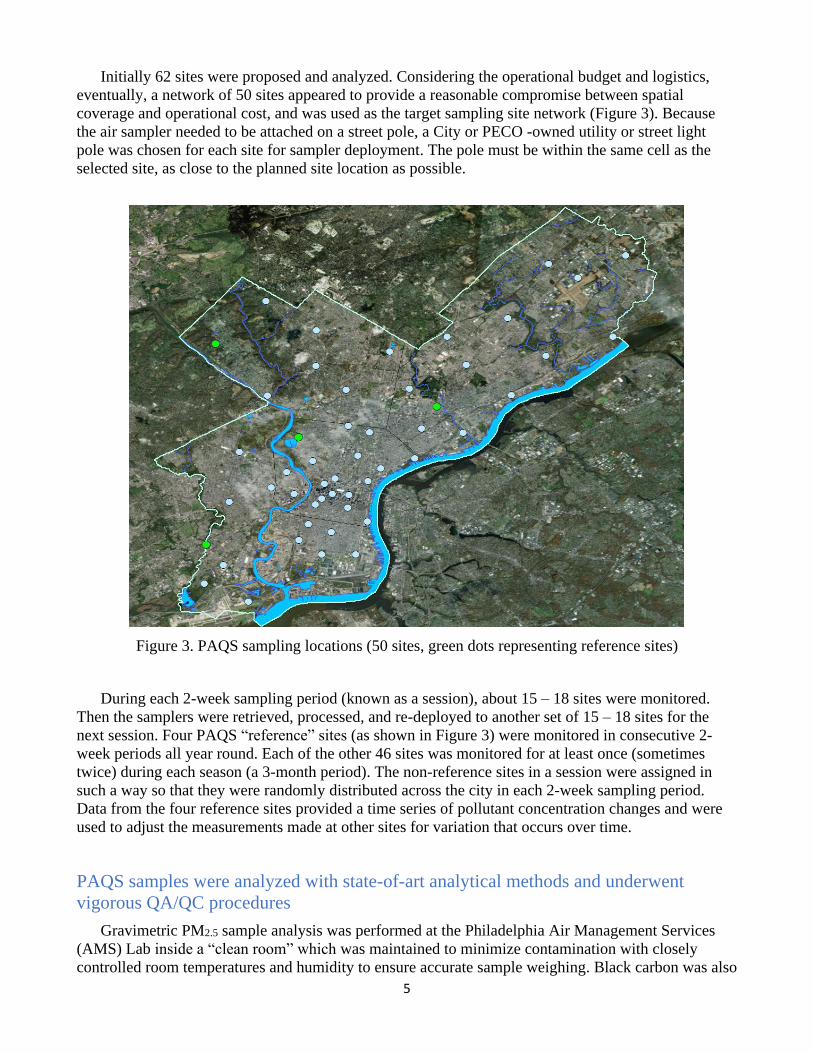
Initially 62 sites were proposed and analyzed. Considering the operational budget and logistics,

eventually, a network of 50 sites appeared to provide a reasonable compromise between spatial

coverage and operational cost, and was used as the target sampling site network (Figure 3). Because

the air sampler needed to be attached on a street pole, a City or PECO -owned utility or street light

pole was chosen for each site for sampler deployment. The pole must be within the same cell as the

selected site, as close to the planned site location as possible.

Figure 3. PAQS sampling locations (50 sites, green dots representing reference sites)

During each 2-week sampling period (known as a session), about 15 – 18 sites were monitored.

Then the samplers were retrieved, processed, and re-deployed to another set of 15 – 18 sites for the

next session. Four PAQS “reference” sites (as shown in Figure 3) were monitored in consecutive 2-

week periods all year round. Each of the other 46 sites was monitored for at least once (sometimes

twice) during each season (a 3-month period). The non-reference sites in a session were assigned in

such a way so that they were randomly distributed across the city in each 2-week sampling period.

Data from the four reference sites provided a time series of pollutant concentration changes and were

used to adjust the measurements made at other sites for variation that occurs over time.

PAQS samples were analyzed with state-of-art analytical methods and underwent

vigorous QA/QC procedures

Gravimetric PM2.5 sample analysis was performed at the Philadelphia Air Management Services

(AMS) Lab inside a “clean room” which was maintained to minimize contamination with closely

controlled room temperatures and humidity to ensure accurate sample weighing. Black carbon was also

6

analyzed at the AMS Lab using an optical carbon analysis method for Teflon filters [14]. The analysis of

the passive samplers of gaseous pollutants was performed by RTI International Laboratories (Research

Triangle Park, NC, USA).

Vigorous quality assurance/quality control (QA/QC) measures were designed and implemented,

including: documentation and procedures (project design documents, quality assurance project plan,

standard operating procedures), PM2.5 air pump flow rate calibration and audit, sample blanks, co-

located samples using two identical PAQS samplers, and co-located samples comparing PAQS with

EPA designated air monitoring methods. Various check lists, data sheets, and log forms were used to

ensure high levels of data quality and record keeping. This practice also proves highly useful in

investigating potential issues.

Results

The first sampling session started on May 9, 2018, mostly serving as a trial run. Full scale

operation followed in June 2018. As of June 2020, 34 two-week sampling sessions were performed.

The data results presented in this report are mostly based on the raw data collected during the two-year

period from early June 2018 through early June 2020. These are preliminary findings as the project

operation is ongoing at the time of this report.

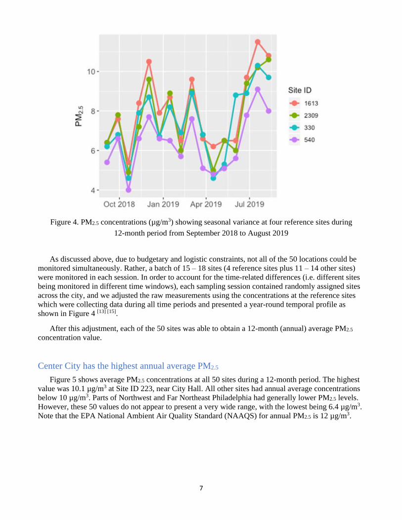
Air quality in Philadelphia is usually worse in Summer and Winter seasons

Air pollution concentrations vary due partly to geographical and emission source related

differences, but also due to weather and other time-varying factors. In terms of seasonal variation, the

PM2.5 concentrations were generally lower in Spring (March, April and May) and Fall (September,

October and November) seasons and higher in Summer (June, July and August) and Winter

(December, January, and February). The graph in Figure 4 demonstrates this season-to-season trend.

The data were collected at the four reference sites during a 12-month period. Each dot in the graph is a

2-week average PM2.5 concentration value in µg/m3.

This seasonal trend agrees with what we have seen in the regulatory monitoring data in

Philadelphia over the years.

7

Figure 4. PM2.5 concentrations (µg/m3) showing seasonal variance at four reference sites during

12-month period from September 2018 to August 2019

As discussed above, due to budgetary and logistic constraints, not all of the 50 locations could be

monitored simultaneously. Rather, a batch of 15 – 18 sites (4 reference sites plus 11 – 14 other sites)

were monitored in each session. In order to account for the time-related differences (i.e. different sites

being monitored in different time windows), each sampling session contained randomly assigned sites

across the city, and we adjusted the raw measurements using the concentrations at the reference sites

which were collecting data during all time periods and presented a year-round temporal profile as

shown in Figure 4 [13] [15].

After this adjustment, each of the 50 sites was able to obtain a 12-month (annual) average PM2.5

concentration value.

Center City has the highest annual average PM2.5

Figure 5 shows average PM2.5 concentrations at all 50 sites during a 12-month period. The highest

value was 10.1 µg/m3 at Site ID 223, near City Hall. All other sites had annual average concentrations

below 10 µg/m3. Parts of Northwest and Far Northeast Philadelphia had generally lower PM2.5 levels.

However, these 50 values do not appear to present a very wide range, with the lowest being 6.4 µg/m3.

Note that the EPA National Ambient Air Quality Standard (NAAQS) for annual PM2.5 is 12 µg/m3.

8

Figure 5. 12-month average PM2.5 concentrations (µg/m3) at 50 sites

(September 2018 – August 2019)

Another 12-month PM2.5 concentration map is shown in Figure 6. This reflects data from June

2019 through May 2020. During this period, the highest value was 9.4 µg/m3 (again, at Site 223, near

City Hall). Most other sites had annual average concentrations below 9 µg/m3. The lowest value was

6.2 µg/m3 at Site 540 (Northwest Philly). Again, parts of Northwest and Far Northeast Philadelphia

had generally lower PM2.5 levels. The citywide all-sites 12-month average concentration was 7.7

µg/m3.

9

Figure 6. 12-month average PM2.5 concentrations (µg/m3) at 50 sites (June 2019 – May 2020)

Figure 7 presents the two-week average PM2.5 concentrations from each sampling session from

June 2018 through June 2020. This represents a two-year period with 33 two-week sampling sessions.

The highest citywide two-week average value was 11.3 µg/m3 (early July 2018) and the lowest

citywide two-week average was 4.6 µg/m3 (early April 2020 during the COVID-19 shutdown period).

10

Figure 7. Citywide two-week average PM2.5 concentrations

11

Similar to annual concentration analysis, a seasonal average PM2.5 concentration value for each site

was obtained for all four seasons, illustrated in Figure 8. The Fall season shown here represents

September – November 2018, Winter for December 2018 – February 2019, Spring for March – May

2019, and Summer for June – August 2019. As discussed above, in general the Fall and Spring seasons

had lower PM2.5 pollution levels than Summer and Winter.

Figure 8. Seasonal average PM2.5 concentrations (µg/m3) at 50 sites

Road traffic is a top factor related to fine particle pollution in Philadelphia

We identified and analyzed multiple air quality related variables to examine their relationships with

fine particle pollution in the city. It was found that road density was a top factor correlated to the PM2.5

levels at different locations. Road density is the total length of roads/streets per square kilometer. It is

related to and an indicator of the volume of vehicle traffic. The road density within 300-meter radius of

a site correlates to about 32% of the variance of PM2.5 concentrations. This means that areas with

higher road density, hence likely higher vehicle traffic volume, tend to have higher PM2.5 levels. It

suggests that road traffic is an important contributor to fine particle pollution in the city. Other factors

include: buildings (which contain pollution sources such as boilers, heaters, vents, etc.), other

12

industrial and commercial combustion sources, population density, etc. Figure 9 is a map of the road

density in each 300x300-meter cell in the city. Figure 10 shows the relations between road density and

PM2.5 concentrations.

Figure 9. Road density in Philadelphia in 300 x 300-meter grid cells

Figure 10. Annual PM2.5 value at a site versus road density within 300-meter radius

showing positive correlation

13

Based on the annual average PM2.5 values, we also calculated an average value for each of the 18

Planning Districts in Philadelphia. The district average value was obtained from weighted average

concentrations at the sites within a district, using a technique known as inverse distance weighting.

With inverse distance weighting a concentration projection at a location is based on all monitoring

locations but the influence of each point is in inverse proportion to the distance away. Figure 11

presents PM2.5 concentration values by planning district. This is based on data collected during

September 2018 through August 2019. The lowest district-wide average concentration was 7.6 µg/m3

and the highest was 8.2 µg/m3, indicating relatively small spatial variance across the City.

Figure 11. Annual average PM2.5 values (µg/m3) by planning district

PM2.5 measurements show satisfactory data quality

When comparing PAQS PM2.5 values with the average values in the same 2-week periods

measured by EPA sponsored regulatory monitors with methods known as Federal Reference Method

and/or Federal Equivalent Method (FRM/FEM), the PAQS values are highly comparable with the

FRM/FEM measurements, indicating satisfactory data quality (Figure 12). In each session, the PAQS

14

maximum PM2.5 value, the minimum PM2.5 value, and the citywide average FRM/FEM value track one

another closely in a similar trend.

Figure 12. PAQS PM2.5 values compared with FRM/FEM measurements

Nitrogen dioxide and ozone measurements

NO2 and Ozone measured in PAQS are presented in Figures 13 and 14. Similar to the PM2.5 data,

PAQS data for NO2 and Ozone also showed concentration levels and trends closely tracking those

indicated by FRM measurements collected at AMS regulatory monitors. NO2 and O3 were sampled at

16 sites (two more sites added in 2019). Most of these sites were in Center City and near traffic

corridors, such as I-95, I-76, Roosevelt Blvd., S. Front Street, Columbus Blvd, etc. Among these sites,

the highest 12-month average NO2 concentration was 20.2 parts per billion (ppb) at Site 223 (City

Hall). The PAQS all-sites average NO2 concentration during the 12-month period was 13.0 ppb, while

the citywide regulatory sites (FRM/FEM) average concentration was 12.8 ppb when comparing data

obtained during the PAQS sampling periods.

Figure 13 illustrates the PAQS maximum NO2 value, the minimum NO2 value, and the City-wide

2-week average FRM value in each session comparing with one another. Note that the EPA National

Ambient Air Quality Standards for NO2 are: (1) 1-hour average not exceeding 100 ppb); and (2) annual

average not exceeding 53 ppb.

Ground level ozone is mainly a summertime air pollution problem. It is formed in the air from

other pollutants (mostly nitrogen oxides and volatile organic compounds) when atmospheric

temperatures are high and sunlight is plenty.

15

Figure 13. PAQS NO2 values compared with FRM measurements

Figure 14 shows the PAQS maximum O3 value, the minimum O3 value, and the citywide 2-week

average FRM value in each session comparing with one another. In this project ozone was measured

during summer times. The EPA National Ambient Air Quality Standard for ozone is: daily maximum

8-hour average concentration not exceeding 70 parts per billion (or 0.07 parts per million).

Figure 14. PAQS O3 values compared with FRM measurements

16

The ambient sulfur dioxide levels in Philadelphia are typically at a few parts per billion according

to AMS regulatory monitoring data. These are well below the EPA National Ambient Air Quality

Standard for SO2 (1-hour concentration not exceeding 75 ppb), as a result of implementation of

federal, state and City regulations that control burning of sulfur-containing fuels. The passive SO2

samplers used in the PAQS project produced data that were about only 10% of the values measured by

the AMS regulatory (FRM) monitors. This indicates that this type of passive SO2 samplers is not

accurate when the ambient SO2 concentrations are low.

Discussion

The PAQS project is helping address public health concerns in neighborhood level air pollutant

concentrations across the City. This type of information was generally unavailable in previous efforts

of air quality monitoring.

The EPA National Emission Inventory data have indicated that vehicular sources account for a

large percentage of air pollution emissions in Philadelphia. For example, nearly 40% of the nitrogen

oxides emitted in the City is from on-road mobile sources. This percentage may become even higher

since a large local stationary source (PES Refinery) has shut down. The PAQS data, coupled with land

use analysis, will provide us with better understanding of how road traffic is linked to emissions of

PM2.5 and NO2. The finding that the Center City area, with heavy and congested vehicle traffic, has the

highest PM2.5 and NO2 levels points to significant pollution contribution from vehicular emission

sources.

17

Because of the widespread geographical locations of the sampling sites across the city, all

pollutants exhibited higher spatial variation among PAQS sites than are captured by AMS regulatory

monitoring sites. When comparing sites with one another, the highest PAQS annual average PM2.5

concentration (Center City) is about 1.6 times the lowest annual average level (Northwest Philly). Still,

for a city the size of Philadelphia, this does not appear to be a very large range of spatial variance.

Temporal trends in two-week average pollutant concentrations were generally consistent between

PAQS and regulatory monitoring data.

The integrated sampling units performed as designed and provided satisfactory air pollutant data

for the purposes of this study. Methods used in PAQS, with relatively lower cost equipment to collect

multi-pollutant samples, are one important approach to urban air pollution monitoring that should be

further studied and explored, with a direction towards making the operation more automated and less

resource intensive. This can be a very useful complement to existing regulatory air quality monitoring.

Implications for public health and emission reduction

Exposure to PM2.5 has been linked to exacerbation of heart and lung diseases, including asthma,

and contributes to hospitalizations, emergency room visits, and work and school absences. NO2 and O3

are respiratory irritants that can worsen respiratory illnesses like asthma, resulting in emergency

department visits and hospitalizations. These pollutants are directly and/or indirectly emitted from

various combustion sources, particularly vehicular sources in Philadelphia. We believe that findings

from PAQS can enhance local stakeholder engagement and contribute to policy making in air quality

improvement. The Philadelphia City Council passed a City Code amendment in 2019 that prohibits

burning of heavy commercial fuel oils (#4, #5, and #6 oils) in the city. A variety of other measures

should be considered and could potentially be implemented to reduce air pollution, such as replacing

diesel powered buses in the city with electric buses, expanding mass transit options to reduce driving

of private cars, supporting retrofits and replacement of diesel-powered trucks and equipment,

switching to new and more efficient boilers and heaters, etc. As observed during the COVID-19

pandemic, reducing vehicle traffic can significantly lower PM2.5 and NO2 pollution levels in

Philadelphia.

18

References

1. U.S. Environmental Protection Agency: NAAQS Table. https://www.epa.gov/criteria-air-

pollutants/naaqs-table. Updated December 20, 2016. Accessed July 22, 2019.

2. U.S. Environmental Protection Agency: 2012 Annual PM2.5 Designations,

https://epa.maps.arcgis.com/apps/MapJournal/index.html?appid=a76e14f777de49baa5d32f5544c8e20b

&webmap=fc297672dd074e4ab5b208aebe21fa52. Updated May 2017. Accessed July 22, 2019.

3. Xing YF, Xu YH, Shi MH, Lian YX: The impact of PM2.5 on the human respiratory system. J

Thorac Dis. 2016;8(1):E69–E74. doi:10.3978/j.issn.2072-1439.2016.01.19

4. Kim D, Chen Z, Zhou LF, Huang SX: Air pollutants and early origins of respiratory diseases.

Chronic Dis Transl Med. 2018;4(2):75–94. Published 2018 Jun 7. doi:10.1016/j.cdtm.2018.03.003

5. Shah AS, Langrish JP, Nair H, et al.: Global association of air pollution and heart failure: a

systematic review and meta-analysis. Lancet. 2013;382(9897):1039–1048. doi:10.1016/S0140-

6736(13)60898-3

6. Pope CA III, Burnett RT, Thurston GD, Thun MJ, Calle EE, Krewski D, Godleski JJ.:

Cardiovascular mortality and long-term exposure to particulate air pollution: epidemiological evidence

of general pathophysiological pathways of disease. Circulation 2004;109:71–77.

7. U.S. Environmental Protection Agency: Quantitative Health Risk Assessment for Particulate Matter.

EPA-452/R-10-005,

https://www3.epa.gov/ttn/naaqs/standards/pm/data/PM_RA_FINAL_June_2010.pdf. Published June

2010. Accessed July 22, 2019.

8. World Health Organization: Regional Office for Europe. Health Effects of Particulate Matter.

http://www.euro.who.int/__data/assets/pdf_file/0006/189051/Health-effects-of-particulate-matter-

final-Eng.pdf. Published 2013. Accessed July 22, 2019.

9. Medina S.: Summary Report of the APHEKOM Project 2008–2011. Saint-Maurice Cedex, Institut

de Veille Sanitaire, 2012 (www.endseurope.com/docs/110302b.pdf, accessed 22 July 2019).

10. Lepeule J, Laden F, Dockery D, Schwartz J.: Chronic exposure to fine particles and mortality: an

extended follow-up of the Harvard Six Cities study from 1974 to 2009. Environ Health Perspect.

2012;120(7):965–970. doi:10.1289/ehp.1104660

11. Correia AW, Pope CA 3rd, Dockery DW, Wang Y, Ezzati M, Dominici F.: Effect of air pollution

control on life expectancy in the United States: an analysis of 545 U.S. counties for the period from

2000 to 2007. Epidemiology. 2013;24(1):23–31. doi:10.1097/EDE.0b013e3182770237

12. U.S. Environmental Protection Agency: OAR (5 June 2015). Health Effects of Ozone

Pollution. US EPA.

13. Matte T., Kheirbek I., et al.: Monitoring intraurban spatial patterns of multiple combustion

pollutants in New York City: Design and implementation. Journal of Exposure Science and Environmental

Epidemiology · January 2013.

19

14. Presler-Jur P., Doraiswamy P., et al.: An evaluation of robotic optical carbon analysis on Teflon

filter media, https://www3.epa.gov/ttnamti1/files/2014conference/wedemergpreslerjur.pdf, RTI

International and US EPA.

15. Ito K, Thurston GD, Silverman RA. Characterization of PM2.5, gaseous pollutants, and

meteorological interactions in the context of time-series health effects models. J Expos Sci Environ

Epidemiol 2007; 17(Suppl 2): S45–S60.